Embed Size (px)
Citation preview
REPORT NUMBER 163
NOVEMBER 1965
PRELIMINARY FLUTTER ANALYSIS
VOLUME II EMPENNAGE
\ /
I _.._J
J 1 I LIFT FAN FLIGHTRES
CONTRACT NUMBER OA44 177-TC-/15.
GENERAL (g) ELECTRIC
NASA Scientific and Technical Information Facility operated for the National Aeronautics and Space Administration by Documentation Incorporated
Post Office Box 33 College Park, Md 20740
Telephonel Area Code 301 | 779-2121
FACILITY CONTROL NO. 'S^^C/
ATTACHED IS A DOCUMENT ON LOAN
FROM: NASA Scientific and Technical Information Facility
TO: Defense Documentation Center Attn: DDC-IRC (Control Branch) Cameron Station Alexandria, Va. 2231**
In accordance with the NASA-DOD Cooperative AD Number Assignment Agreement it is requested that an AD number be assigned to the attached report.
B As this is our only available copy the return of the document (with AD number and any applicable distribution linitatlons) to the address below is essential.
D This document may be retained by ODC. If retained, please indicate AD number and any applicable distribution limitations on the reproduced copy of the title page and return to the address below.
Return Address: NASA Scientific and Technical Information Facility Attention: INPUT BRANCH P. 0. Box 33 College Park, Maryland 20740
FFNo 2kk Revised Aug 65
■»"
>alw la . -..i>#*J
lieöwiwur mn wHiii tSTM
ODC <».' f WD
J> I ICUOli
tVFFSBTIM i Report Nusber 163
ei;Ti B0Ti«i7*wiuiiun COBES
OUT. I AVAIL. Ml/Of »EGIALI
PRELIMINARY FLUTTER ANALYSIS
VOLUME II - EMPENNAGE
XV-5A Lift Pan Plight Research Aircraft
Contract DA 44-177-TC-715
Decenber 1965
ADVANCED ENGINE k TECHNOLOGY DEPARTMENT GENERAL ELECTRIC COMPANY CINCINNATI, OHIO 45215
(I> H CD Q
s H
CO
i
r
■b-..'.. LiA<1 ■
CONTENTS
SECTION
1.0 SUMMARY
2.0 INTRODUCTION
3.0 METHOD OF APPROACH
3.1 Lagrange's Equations of Motion
3.1.1 Generalized Mass Matrix
3.1.2 Generalized StiffneBB Matrix
3.1.3 Generalized Aerodynamic Matrix
3.2 Symmetric Flutter Analysis
3.2.1 Cantilevered
3.2.1.1 Generalized Mass Matrix
3.2.1.2 Generalized Aerodynamic Matrix
3.2.2 Free-Free
3.2.2 1 Generalized Mass Matrix
3.2.2.2 Generalized Aerodynamic Matrix
3.3 Antisymmetric Flutter Analysis
3.3.1 Cantilevered
3.3.1.1 Generalized Mass Matrix
3.3.1.2 Generalized Aerodynamic Matrix
3.3.2 Free-Free
3.3.2.1 Modal Coupling
3.3.2.2 Flutter Analysis
PAGE
1
3
5
5
7
18
20
26
26
26
27
28
26
30
30
30
31
32
32
33
36
iii
CONTENTS (Continued)
SECTION
4.0 DISCUSSION AND RESULTS
4.1 Idealization of Aircraft
4.1.1 Structural Representation
4.1.1.1 Horizontal Stabilizer - Elevator
4.1.1.2 Vertical Stabilizer - Rudder
4.1.1.3 Fuselage
4.1.2 Aerodynamic Representation
4.1.2.1 Empennage
4.1.3 Mass Representation
4.1.3.1 Symmetric Analysis
4.1.3.2 Antisymmetric Analysis
4.2 Modal Functions
4.2.1 Symmetric Analysis
4.2.1.1 Canlilevered
4.2.1.2 Free-Free
4.2.2 Antisymmetric Analysis
4.2.2.1 Cantilevered
4.2.2.2 Free-Free
4.3 Flutter Analysis
4.3.1 Symmetric
4.3.1.1 Cantilevered Analysis
4.3.1.2 Free-Free Analysis
4.3.2 Antisymmetric
4.3.2.1 Cantilevered Analysis
4.3.2.2 Free-Free Analysis
PAGE
39
39
39
39
40
40
40
40
41
41
41
42
42
42
42
42
43
43
43
44
44
46
46
46
47
iv
htm A- u*»..
CONTENTS (Continued)
SECTION PAGE
5.0 CONCLUSIONS
5.1 Symmetric Analysis - Cantilevered Condition 49
5.2 Symmetric Analysis - Free-Free Condition 50
5.3 Antisymmetric Analysis - Cantilevered 51 Condition
5.4 Antisymmetric Analysis - Free-Free 51 Condition
5.5 Overall Evaluation 51
6.0 APPENDIX
6.1 List of References 53
B. 2 Tables 54
6.3 Figures 6 through 69 65
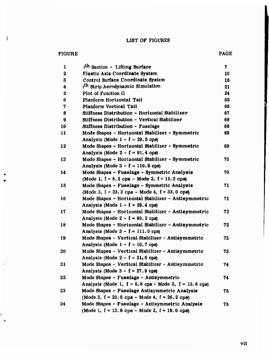
LIST OF FIGURES
FIGURE PAGE
1 Ith Section - Lifting Surface 7 2 Elastic Axis Coordinate System 10 3 Control Surface Coordinate System 15 4 ittl Strip Aerodynamic Simulation 21 5 Plot of Function G 24 6 Planform Horizontal Tail 65 7 Planform Vertical Tail 66 8 Stiffness Distribution - Horizontal Stabilizer 67 9 Stiffness Distribution - Vertical Stabilizer 68
10 Stiffness Distribution - Fuselage 68 11 Mode Shapes - Horizontal Stabilizer - Symmetric 69
Analysis (Mode 1 - f = 29.5 cps) 12 Mode Shapes - Horizontal Stabilizer - Symmetric 69
Analysis (Mode 2 - f = 91.4 cps) 13 Mode Shapes - Horizontal Stabilizer - Symmetric 70
Analysis (Mode 3 - f = 110.9 cps) 14 Mode Shapes - Fuselage - Symmetric Analysis 70
(Mode 1, f = B. 2 cps - Mode 2. f = 15.2 cps) 15 Mode Shapes - Fuselage - Symmetric Analysis 71
(Mode 3, f = 23. 2 cps - Mode 4, f = 33.0 cps) 16 Mode Shapes - Horizontal Stabilizer - Antisymmetric 71
Analysis (Mode 1 - f = 29.4 cps) 17 Mode Shapes - Horizontal Stabilizer - Antisymmetric 72
Analysis (Mode 2 - f > 90. 2 cps) 18 Mode Shapes - Horizontal Stabilizer - Antisymmetric 72
Analysis (Mode 3 - f = 111.0 cps) 19 Mode Shapes - Vertical Stabilizer - Antisymmetric 73
Analysis (Mode 1 - f = 10.7 cps) 20 Mode Shapes - Vertical Stabilizer - Antisymmetric 73
Analysis (Mode 2 - f = 21,6 cps) 21 Mode Shapes - Vertical Stabilizer - Antisymmetric 74
Analysis (Mode 3 - f = 27.9 cps) 22 Mode Shapes - Fuselage - Antisymmetric 74
Analysis (Mode 1, f = 5.6 cps - Mode 2, f = 13.6 cps) 23 Mode Shapes - Fuselage Antisymmetric Analysis 75
(Mode 3, f = 20.6 cps - Mode 4. f = 26. 2 cps) 24 Mode Shapes - Fuselage - Antisymmetric Analysis 75
(Mode 1, f = 13.9 cps - Mode 2, f = 19.0 cps)
vii

* • " I
BLANK PAGE
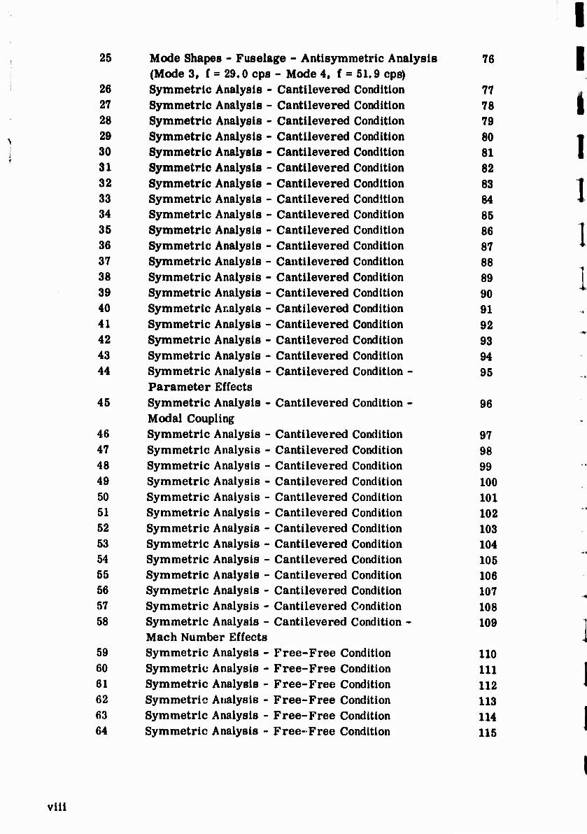
, 25 Mode Shapes - Fuselage - Antisymmetric Analysis 76 (Mode 3, f = 29.0 cps - Mode 4, f = 51.9 ops)
26 Symmetric Analysis - Cantilevered Condition 77 27 Symmetric Analysis - Cantilevered Condition 78 28 Symmetric Analysis - Cantilevered Condition 79
> 29 Symmetric Analysis - Cantilevered Condition 80 30 Symmetric Analysis - Cantilevered Condition 81 31 Symmetric Analysis - Cantilevered Condition 82 32 Symmetric Analysis - Cantilevered Condition 83 33 Symmetric Analysis - Cantilevered Condition 84 34 Symmetric Analysis - Cantilevered Condition 85 35 Symmetric Analysis - Cantilevered Condition 86 36 Symmetric Analysis - Cantilevered Condition 87 37 Symmetric Analysis - Cantilevered Condition 88 38 Symmetric Analysis - Cantilevered Condition 89 39 Symmetric Analysis - Cantilevered Condition 90 40 Symmetric Analysis - Cantilevered Condition 91 41 Symmetric Analysis - Cantilevered Condition 92 42 Symmetric Analysis - Cantilevered Condition 93 43 Symmetric Analysis - Cantilevered Condition 94 44 Symmetric Analysis - Cantilevered Condition - 95
Parameter Effects 45 Symmetric Analysis - Cantilevered Condition - 96
Modal Coupling 46 Symmetric Analysis - Cantilevered Condition 97 47 Symmetric Analysis - Cantilevered Condition 98 48 Symmetric Analysis - Cantilevered Condition 99 49 Symmetric Analysis - Cantilevered Condition 100 50 Symmetric Analysis - Cantilevered Condition 101 51 Symmetric Analysis - Cantilevered Condition 102 52 Symmetric Analysis - Cantilevered Condition 103 53 Symmetric Analysis - Cantilevered Condition 104 54 Symmetric Analysis - Cantilevered Condition 105 55 Symmetric Analysis - Cantilevered Condition 106 56 Symmetric Analysis - Cantilevered Condition 107 57 Symmetric Analysis - Cantilevered Condition 108 58 Symmetric Analysis - Cantilevered Condition - 109
Mach Number Effects 59 Symmetric Analysis - Free-Free Condition 110 60 Symmetric Analysis - Free-Free Condition 111 61 Symmetric Analysis - Free-Free Condition 112 62 Symmetric Analysis - Free-Free Condition 113 63 Symmetric Analysis - Free-Free Condition 114 64 Symmetric Analysis - Free-Free Condition 115
viii
65 Symmetrie Analysis - Free-Free Condition - 116 Parameter Effects
66 Antisymmetric Analysis - Cantilevered Condition 117 67 Antisymmetric Analysis - Cantilevered Condition 118 68 Antisymmetric Analysis - Free-Free Condition 119 69 Antisymmetric Analysis - Free-Free Condition 120
ix
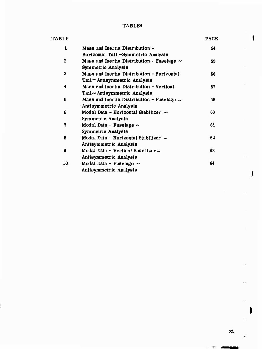
TABLES
TABLE PAGE
1 Mass and Inertia Distribution - 54 Horizontal Tail ^Symmetric Analysis
2 Mass and Inertia Distribution - Fuselage ~ 55 Symmetric Analysis
3 Mass and Inertia Distribution - Horizontal 56 Tail ~ Antisymmetric Analysis
4 Mass and Inertia Distribution - Vertical 57 Tail ~ Antisymmetric Analysis
5 Mass and Inertia Distribution - Fuselage ~ 58 Antisymmetric Analysis
6 Modal Data - Horizontal Stabilizer ~ 60 Symmetric Analysis
7 Modal Data - Fuselage ~ 61 Symmetric Analysis
8 Modal Data - Horizontal Stabilizer ~ 62 Antisymmetric Analysis
9 Modal Data - Vertical Stabilizer ~ 63 Antisymmetric Analysis
10 Modal Data - Fuselage ~ 64 Antisymmetric Analysis
>
xi
■1
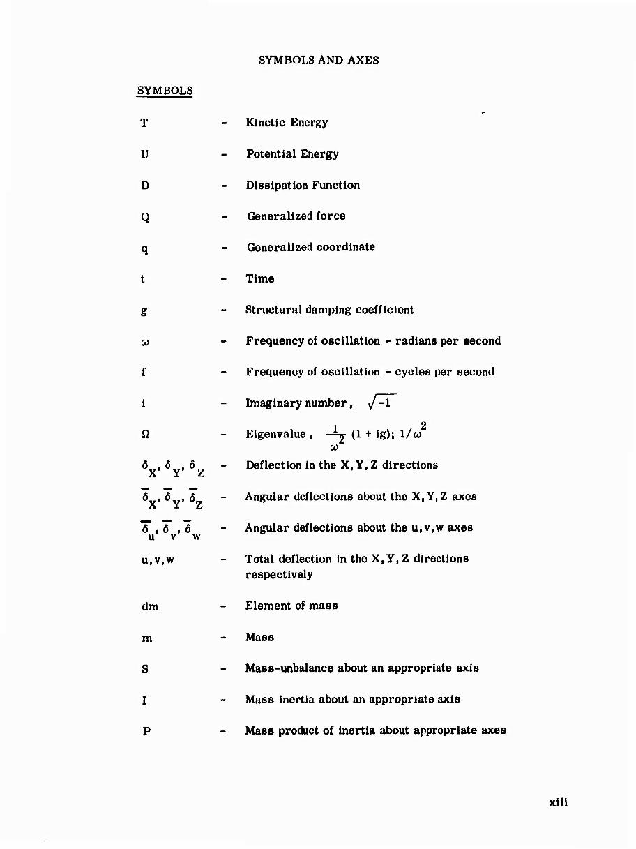
SYMBOLS AND AXES
SYMBOLS
T - Kinetic Energy
U - Potential Energy
D - Dissipation Function
Q - Generalized force
q - Generalized coordinate
t - Time
g - Structural damping coefficient
w - Frequency of oscillation - radians per second
f - Frequency of oscillation - cycles per second
i - Imaginary number, /-l
2 fi - Eigenvalue , -^ (1 + ig); 1/co
ö » Ö » 6 - Deflection in the X,Y,Z directions
6 i övi 6™ - Angular deflections about the X,Y,Z axes
T , 6 , 6 - Angular deflections about the u,v,w axes u v w
u,v,w - Total deflection in the X,Y,Z directions respectively
dm - Element of mass
m - Mass
S - Mass-unbalance about an appropriate axis
I - Mass inertia about an appropriate axis
P - Mass product of inertia about appropriate axes
xiii
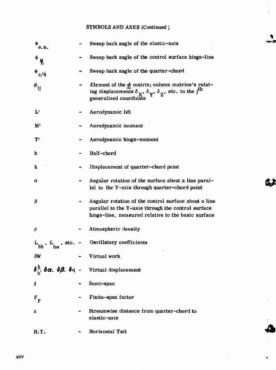
SYMBOLS AND AXES (Continued )
^ - Sweep back angle of the elastic-axis e» a«
\|/ - Sweep back angle of the control surface hinge-line
♦ , - Sweep back angle of the quarter-chord
6,, - Element of the <^ matrix; column matrice's relat- il th ing displacements 6 , 6 , Ö , etc. to the j
generalized coordinate
L' - Aerodynamic lift
M* - Aerodynamic moment
T' - Aerodynamic hinge-moment
b - Half-chord
h - Displacement of quarter-chord point
a - Angular rotation of the surface about a line paral- lel to the Y-axis through quarter-chord point
ß - Angular rotation of the control surface about a line parallel to the Y-axis through the control surface hinge-line, measured relative to the basic surface
p - Atmospheric density
L , L , etc. - Oscillatory coefficients hh ha
ÖW - Virtual work
6~, ÖOt, 6ß, dq - Virtual displacement
i - Semi-span
F - Finite-span factor
a - Streamwise distance from quarter-chord to elastic-axis
H.T. - Horizontal Tail
xlv
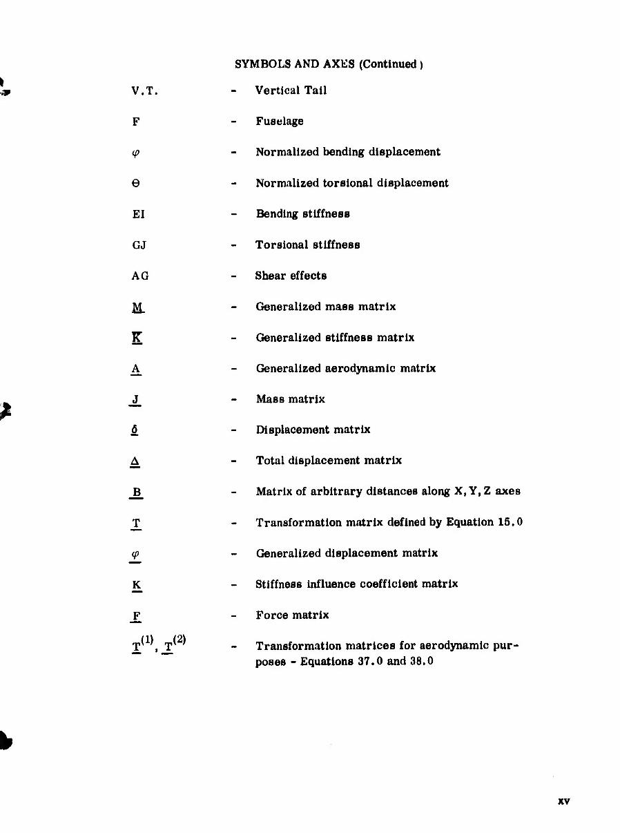
SYMBOLS AND AXES (Continued )
V.T. - Vertical Tail
F - Fuselage
(p - Normalized bending displacement
6 - Normalized torsional displacement
El - Bending stiffness
GJ - Torsional stiffness
AG - Shear effects
HI - Generalized mass matrix
K - Generalized stiffness matrix
A^ - Generalized aerodynamic matrix
_J_ - Mass matrix
6 - Displacement matrix
A^ - Total displacement matrix
B - Matrix of arbitrary distances along X, Y, Z axes
T^ - Transformation matrix defined by Equation 15.0
cp - Generalized displacement matrix
It - Stiffness influence coefficient matrix
_F - Force matrix
T , JT - Transformation matrices for aerodynamic pur- poses - Equations 37.0 and 38.0
xv
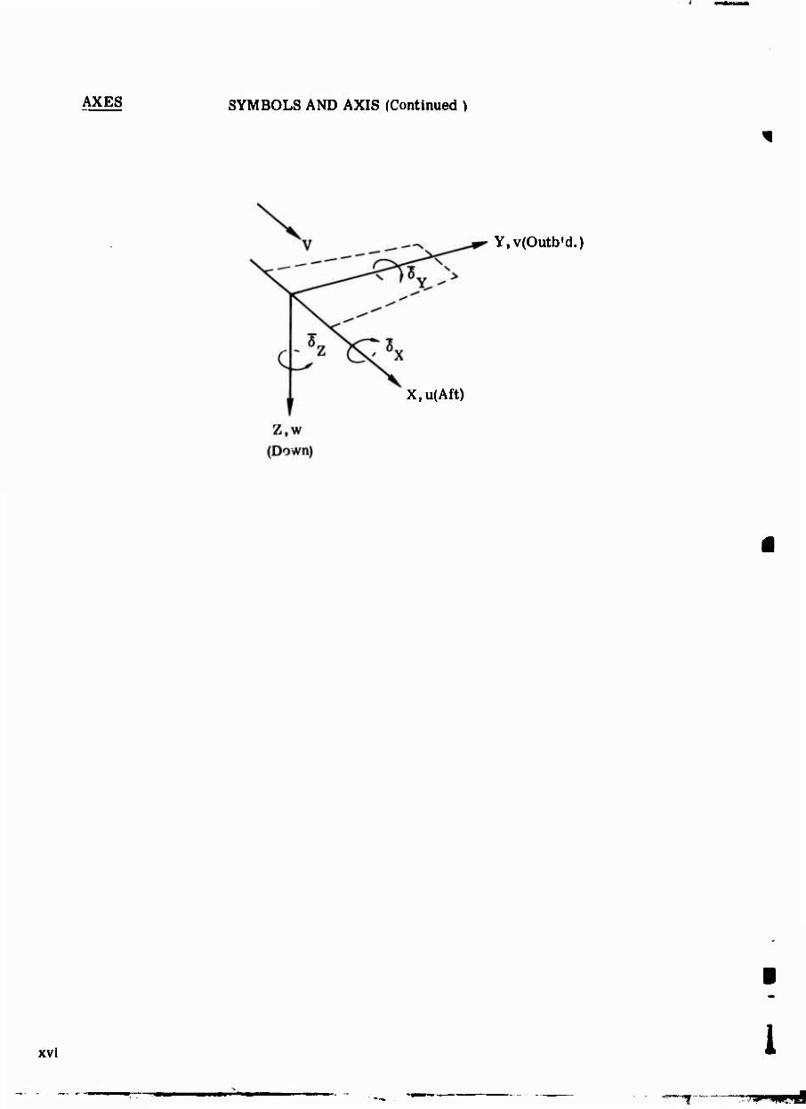
AXES SYMBOLS AND AXIS (Continued )
Y,v(Outb'd.)
X,u(Aft)
xvl I ~7S
1.0 SUimARY
The overall preliminary theoretical flutter analysis of the Ryan XV-5A Lift Fan Aircraft is presented in three volumes. This is Volume II, which reports the investigation of the flutter charac- teristics of the empennage. Volumes I and III detail the analysis of the wing and control surfaces, respectively.
Results of the empennage flutter analysis indicate a possible flutter situation existing within the design flight envelope of the XV-5A aircraft. The flutter mode is characterized by horizontal tail pitch coupled with basically symmetric horizontal tail bending for low values of pitch frequencies (40 cps) and for pitch coupled with horizontal tail torsion at pitch frequencies greater than 40 cps. The required pitch frequency would be of the order of approximately 55 cps for a flutter velocity margin of 15% of the design limit dive speed at sea-level, which is the critical altitude. Establishment of the actual pitch frequency through experimental methods is required for definite determination of flutter margins. The analyses presented in this report should be taken as a preliminary evaluation of the empennage of the XV-5A aircraft. Subsequent analytical and experimental investigations should then be directed toward finalization of the actual flutter characteristics of the XV-5A aircraft, with due regard for the findings of the studies presented in this report.
.■■ M
2.0 INTRODUCTION
Thif report pretentt the results of the preliminary empennage flutter analysis of the U. 8. Army XV-6A lift Fan Research Aircraft, Illustrated in Figure 1.0 of Reference 1. The XV-5A is a V/STOL aircraft designed for research flight testing of the General Electric X-363-S Lift Fan Propulsion System.
The XV-SA aircraft is characterized by the existence of a T-tall with manual type« conventional aerodynamic control surfaces (elevator and rudder). Such tails are prone to exhibit flutter instabilities, unless extreme care is taken during the design stages to insure a flutter-free structure. Further difficulties are presented due to the fact that the horizontal tall is pivoted to provide for longitudinal trim and Is powered by an irreversible Jaokscrew with power applied to the Jaokscrew through hydraulic circuits.
The analysis of the empennage was facilitated by the use of simple beam idealization of the horizontal and vertical stabilizers and fuse- lage. Aerodynamic representation was accomplished through the use of two-dimensional strip theory. Parametric investigations of Important items such as the horizontal tail pitch frequency, elevator and rudder rotational frequency, and horizontal tall rigid body yaw and roll were carried out for establishment of critical areas.
ö. 0 METHOD OF APPROACH
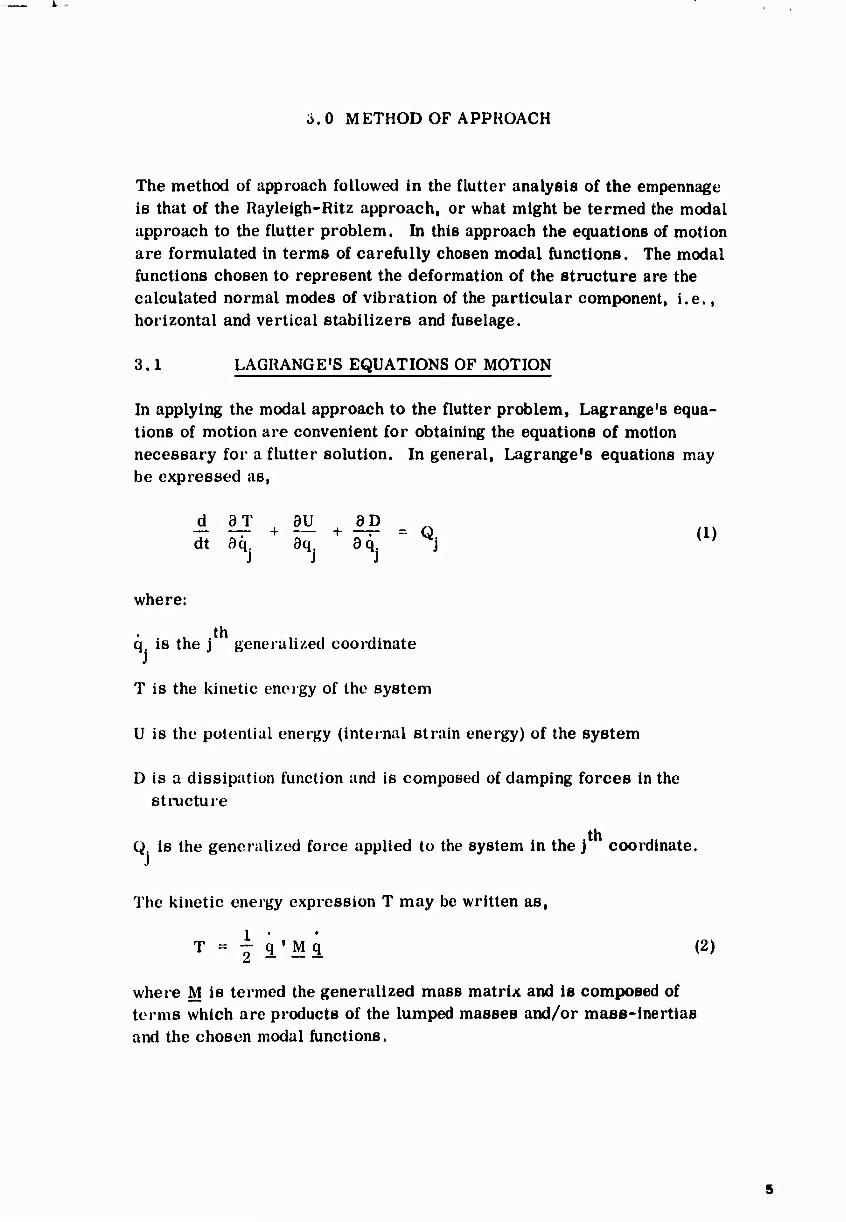
The method of approach followed in the flutter analysis of the empennage is that of the Rayleigh-Ritz approach, or what might be termed the modal approach to the flutter problem. In this approach the equations of motion are formulated in terms of carefully chosen modal functions. The modal functions chosen to represent the deformation of the structure are the calculated normal modes of vibration of the particular component, i.e., horizontal and vertical stabilizers and fuselage.
3.1 LAGRANGE'S EQUATIONS OF MOTION
In applying the modal approach to the flutter problem, Lagrange's equa- tions of motion are convenient for obtaining the equations of motion necessary for a flutter solution. In general, Lagrange's equations may be expressed as,
d 8T 8U 8D ^ dt aq. Bq. aq. j K '
J J J
where:
q is the j generalized coordinate
T is the kinetic energy of the system
U is the potential energy (internal strain energy) of the system
D is a dissipation function and is composed of damping forces in the structure
Q. is the generalized force applied to the system in the j coordinate.
The kinetic energy expression T may be written as,
where M is termed the generalized mass matrix and is composed of terms which are products of the lumped masses and/or mass-inertias and the chosen modal functions.
The potential energy expression U may be written as
U = | q'Kq (3)
where K is termed the generalized stiffness matrix and is composed of terms which are products of the frequency of oscillation squared of a particular mode and its appropriate generalized mass.
The dissipation function D is due to the damping forces acting in the structure. These may be considered as forces in phase with the velocity and proportional to the restoring forces acting in the structure. There- fore,
where g is the coefficient of structural damping and w is the frequency of oscillation.
The generalized force Q* is due to the oscillatory aerodynamics acting on the structure and, for all force components j, Q. may be written as,
^ = co Aa (5)
where A is called the generalized aerodynamic matrix.
Applying Equation 1 to Equations 2, 3, 4, and 5, and assuming harmonic moation (q = q^ wt), the equations of motion for a flutter solution are,
2 — — 2 -co Mc[ + K^ +igKc[ = co Aq
or
CO6 CO
Rearranging,
M + A--^(l+ig)k)ä-o
k -
or (M+A - nK)q = o (6)
where U - 1/w (1 + ig).
For a solution to exist, the determinant of the matrix of Equation 6 must be equal to zero, i.e.,
|M +A-n K | = o (7)
Solution of Equation 7 by standard means yields the required complex eigenvalues from which the flutter speed, frequency and damping values are determined.
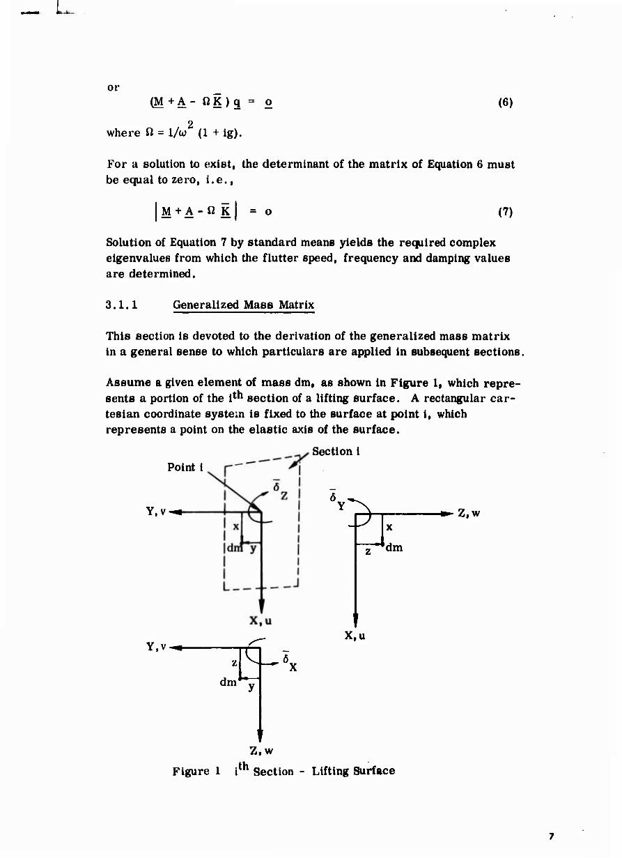
3.1.1 Generalized Mass Matrix
This section is devoted to the derivation of the generalized mass matrix in a general sense to which particulars are applied in subsequent sections.
Assume a given element of mass dm, as shown in Figure 1, which repre- sents a portion of the i**1 section of a lifting surface. A rectangular car- tesian coordinate system is fixed to the surface at point i, which represents a point on the elastic axis of the surface.
Point i
Y.v
Section i
Y.v z
dm
> x
dm
X,u
Z,w
Figure 1 ith Section - Lifting Surface
Z,w
. ..
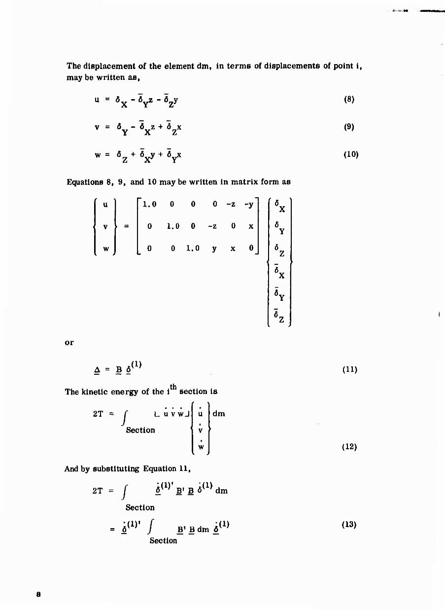
The displacement of the element dm, in terms of displacements of point i, may be written as,
u = öx' v ■ V
v = W+ÖZX
w - öz + ö
xy + ^y*
Equations 8, 9, and 10 may be written in matrix form as
f \ u
w V ^
' —
1.0 0 0 0 -z -y
0 1.0 0 -z 0 x
0 0 1.0 y x 0
or
A = B ö (1)
th The kinetic energy of the i section is
2T = • • •
r L u v wj
Section
u
v
w
dm
And by substituting Equation 11,
2T = T Ö*1* B« B 6(1> dm
Section
= -^ I B1 B dm ö(1)
Section
(8)
(9)
(10)
(11)
(12)
(13)
8
■H*«U r:
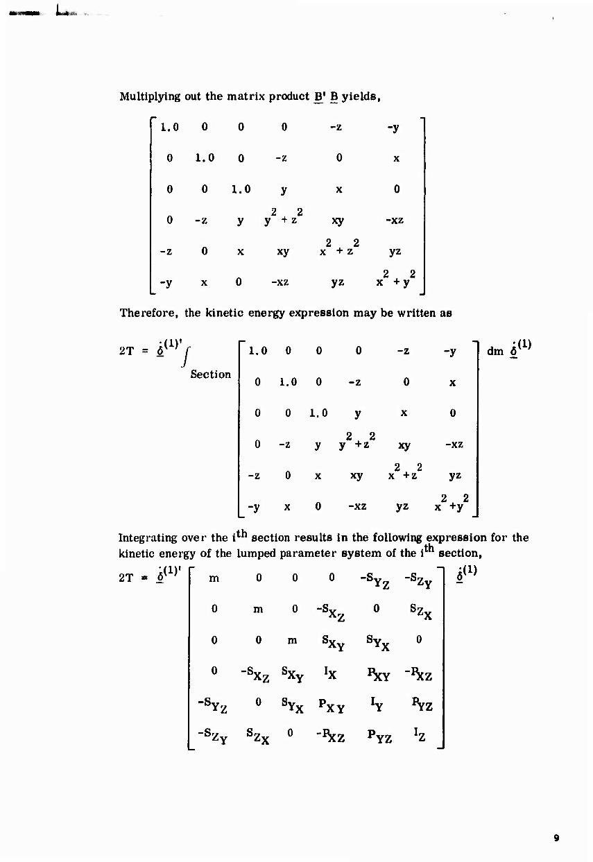
Multiplying out the matrix product B* B yields,
1.0 0
0 1.0 0 -z
-z
0
-y
o
o
-z
-y
o 1.0
-z
0
y 2
y + 2
z xy -xz
X xy 2x 2
x + z yz
0 -xz yz 2. 2 x +y
Therefore, the kinetic energy expression may be written as
2T = ö(1)lr
Section
1.0 0 0 0
0 1.0 0 -z
0 0 1.0
-z
0
-y
o
0 -z y 2 2
y +z xy -xz
z 0 X xy 2 2
X +z yz
y x 0 -xz yz 2.u 2 x +y
dm 6 i(l)
Integrating over the i"1 section results in the following expression for the kinetic energy of the lumped parameter system of the ith section,
2T kW m 0 0 0 -SYZ -HY
0 m 0 -Sxz 0 8H 0 0 m SXY svx
0
0 -sxz SXY "x %Y "^z
Yz 0 ^x PXY •Y ^z -s
-Sv.. Sry.. 0 -I^g •zY °Zx YZ
;(i)
2T = iW' J(1» «(1>
or
where
m
Ix, Iy, Iz
P P P XY* XZ' YZ
s . s Ay Äz
(14)
is the mass of section i lumped at station i
is the mass moment of inertia of section i about the X, Y, Z axes, respectively
is the mass product of inertia of section i about the X-Y, X-Z, and Y-Z axes, respectively
is the static mass moment of section i about the X-axis, with distances measured along the Y and Z axes, respectively
S . S Y ' Y
X Z is the static mass moment of section i about the Y-axis, with distances measured along the X and Z axes, respectively
S . S Z ' Z
X Y is the static mass moment of section i about the Z-axis, with distances measured along the X and Y axes, respectively.
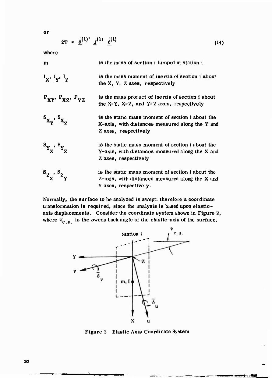
Normally, the surface to be analyzed is swept; therefore a coordinate transformation is required, since the analysis is based upon elastic- axis displacements. Consider the coordinate system shown in Figure 2, where *, e.a. is the sweep back angle of the elastic-axis of the surface.
1 e.a.
Figure 2 Elastic Axis Coordinate System
10
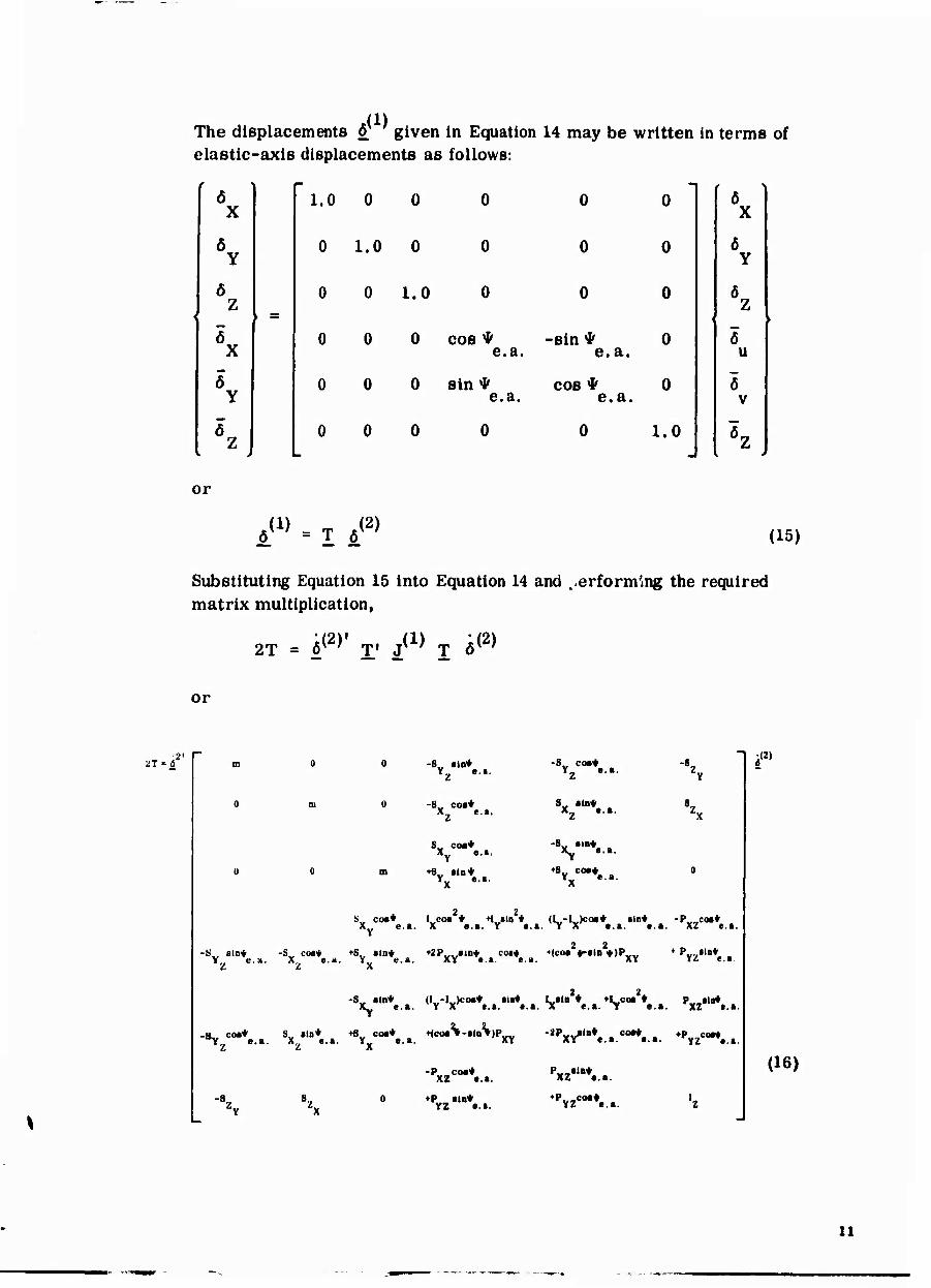
The displacements Ö given in Equation 14 may be written in terms of elastic-axis displacements as follows:
x
1.0 0 0 0 0 0
Y 0 1.0 0 0 0 0
ö ) Z
0 0 1.0 0 0 0 • =
\\ 0 0 0 cos *
e.a. -sin*
e.a. 0
Y 0 0 0 sin *
e.a. cos *
e.a. 0
V 3
0 0 0 0 0 1.0
u
or
ö(1) = T ö
(2) (15)
Substituting Equation 15 into Equation 14 and performing the required matrix multiplication,
2T = i*2»' T- J(1) T «(2)
or
21 '6 2<
-8V »ID* Yz ....
-Sv co»* xz ....
Sv oo»* xY .... ♦«„ »ID*
Yx ....
-8„ co»* Yz ....
Sv »in* xz ....
t8YxC0,*..a.
Sv co»* L-Co»2* ♦lw»ln2* (l^-L.jco»* «in* -Pv_co»* . X e.«. X .... Y .... r X .... .... XZ e...
2 2 -S„ stn* -S„ co.* +SV »In« ♦2PV-,»ID* co»* Mco» i|r»ln ♦)PVV Y e.a. X e.a. Y e.a. XY .... e.a. XY
♦ P„„»ln* YZ e...
pxz*lBV..
-«Y.00'*.... sx."n*.... ^Y,00-*.... ^"^»n -2,,xY"n*....00W.... ♦'YZ8"**...
-P„„co»* XZ ....
♦P„„ »in* YZ ...
XZ ».».
♦P co»* YZ ....
;(2)
(16)
11
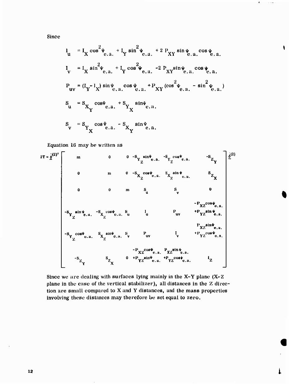
Since
2 2 1 = I„ cos * + I sin * +2 P„„ sin * cos * u X e.a, Y e.u. XY e.a. e.a.
2 2 I = Lr sin * + I„ cos * -2 P, sin^ cos^ v X e.a. Y e.a. XY e.a. e.a.
2 2 P = (I -1,,) sin* cos* +P,,„(cos * -sin * )
uv Y X e.a. e.a. XY e.a. e.a.'
S = S„ cos* + S,r sin* u X e.a. Y e.a.
Y -X
S =S cos* - S,, sin* v Y e.a. X e.a.
Equation 16 may be written as
o 2T « ö(2) m 0 -S,, sin* -S„ COB* Y e.a. Y e.a.
m 0 -S„ COB* S„ Bin* z e"a' % üa-
m
Z.
-S„ sin* -Sv COB* 8 Y e.a. X e.u. u
-S COB* S.F Bin* S Y o.a. X e.u. v
uv
uv
-P COB4 XZ e.a.
y/ e.a.
Pv,7Bin* XZ e.u,
+P cos* YZ e.a.
Z.
-P., .COB* P„, Bin* XZ e.u. XZ e.a.
S,. 0 +P,.,.Bln* +P„„co8* Z YZ e.a. YZ e.a. Z
i(2)
Since we are dealing with surfaces lying mainly in the X-Y plane (X-Z plane in the case of the vertical stabilizer), all distances in the Z direc- tion are small compared to X and Y distances, and the mass properties involving these distances may therefore be set equal to zero.
12 i
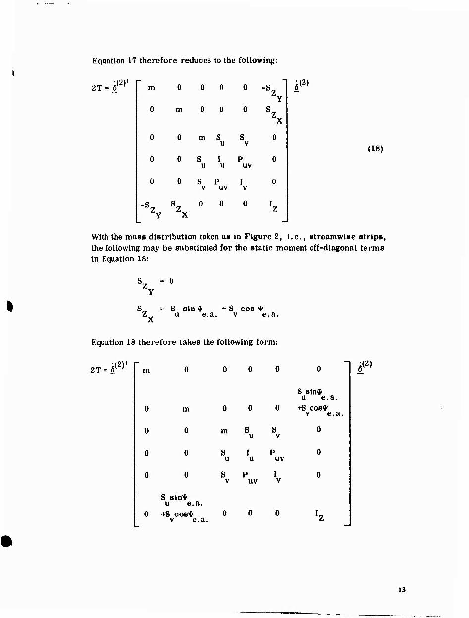
Equation 17 therefore reduces to the following:
•(2)' 2T = öK ' m 0 0 0 0 -S
0 m 0 Ü 0
0 0 m s u
S V
0
0 0 S u
I u
p uv
0
0 0 S V
P uv \
0
\ \
0 0 0 'z
i(2)
(18)
With the mass distribution taken as in Figure 2, i.e., streamwise strips, the following may be substituted for the static moment off-diagonal terms in Equation 18:
S = 0 Z
Y
S^ = S sin * + S cos * Z u e.a. v e.a.
2\
Equation 18 therefore takes the following form:
2T - 6{2)' m
0
0
0
0
0
0
m
0
0
0
S sin* u e.a.
+S cos* v e.a.
0 0
0
S u
0
m S u
u
uv
0 0
0
S
uv
S sin* u e.a. +S cos*
v e.a.
0
0
;(2)
13
or
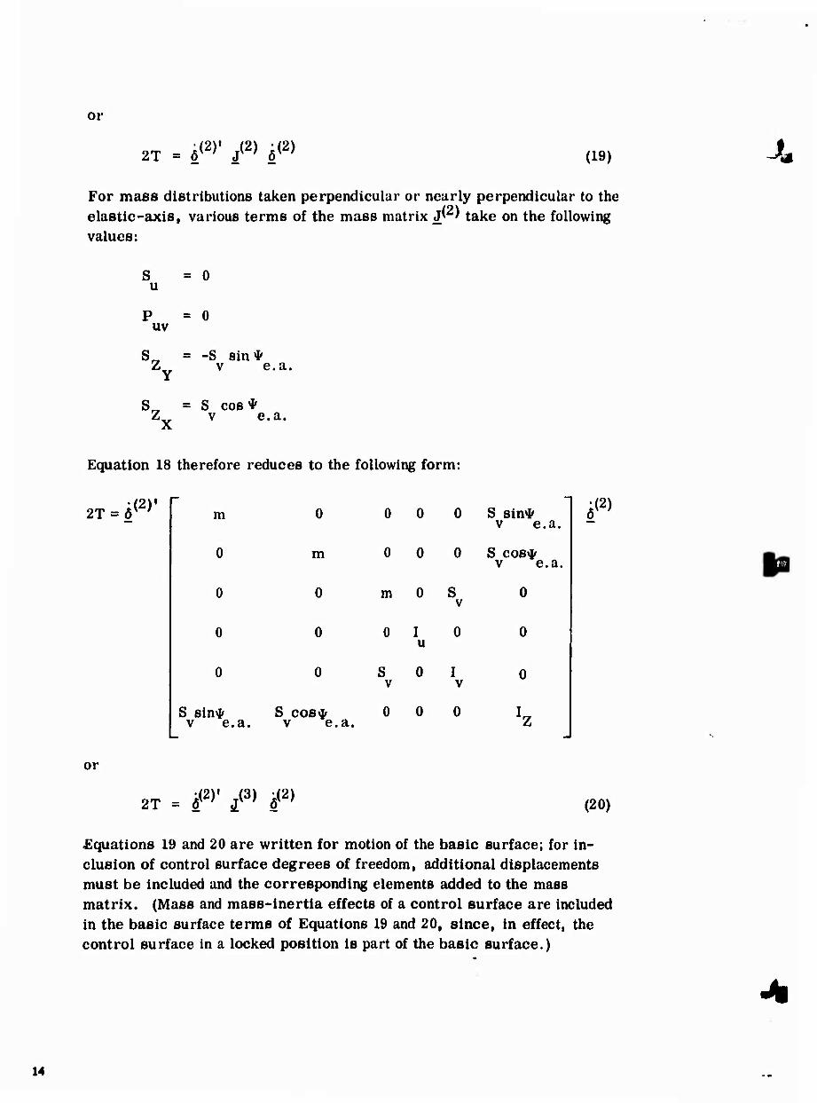
2T = öW J<2> ö<2> (19)
For mass distributions taken perpendicular or nearly perpendicular to the elastic-axis, various terms of the mass matrix J^ ' take on the following values:
S u
uv
0
0
-S sin * v e.a.
S cos* v e.a.
Equation 18 therefore reduces to the following form:
2T = Ö(2)f m 0 0 0 0 S sin* v e.a.
0 m 0 0 0 S cos* v e.a
0 0 m 0 S v
0
0 0 0 I u
0 0
0 0 S v
0 I V
0
S sin* v e.a.
S cos* v e.a.
0 0 0 'z
;(2)
or
2T = ^ ^ 6<2) (20)
Equations 19 and 20 are written for motion of the basic surface; for in- elusion of control surface degrees of freedom, additional displacements must be included and the corresponding elements added to the mass matrix. (Mass and mass-inertia effects of a control surface are included in the basic surface terms of Equations 19 and 20, since, in effect, the control surface in a locked position is part of the basic surface.)
14
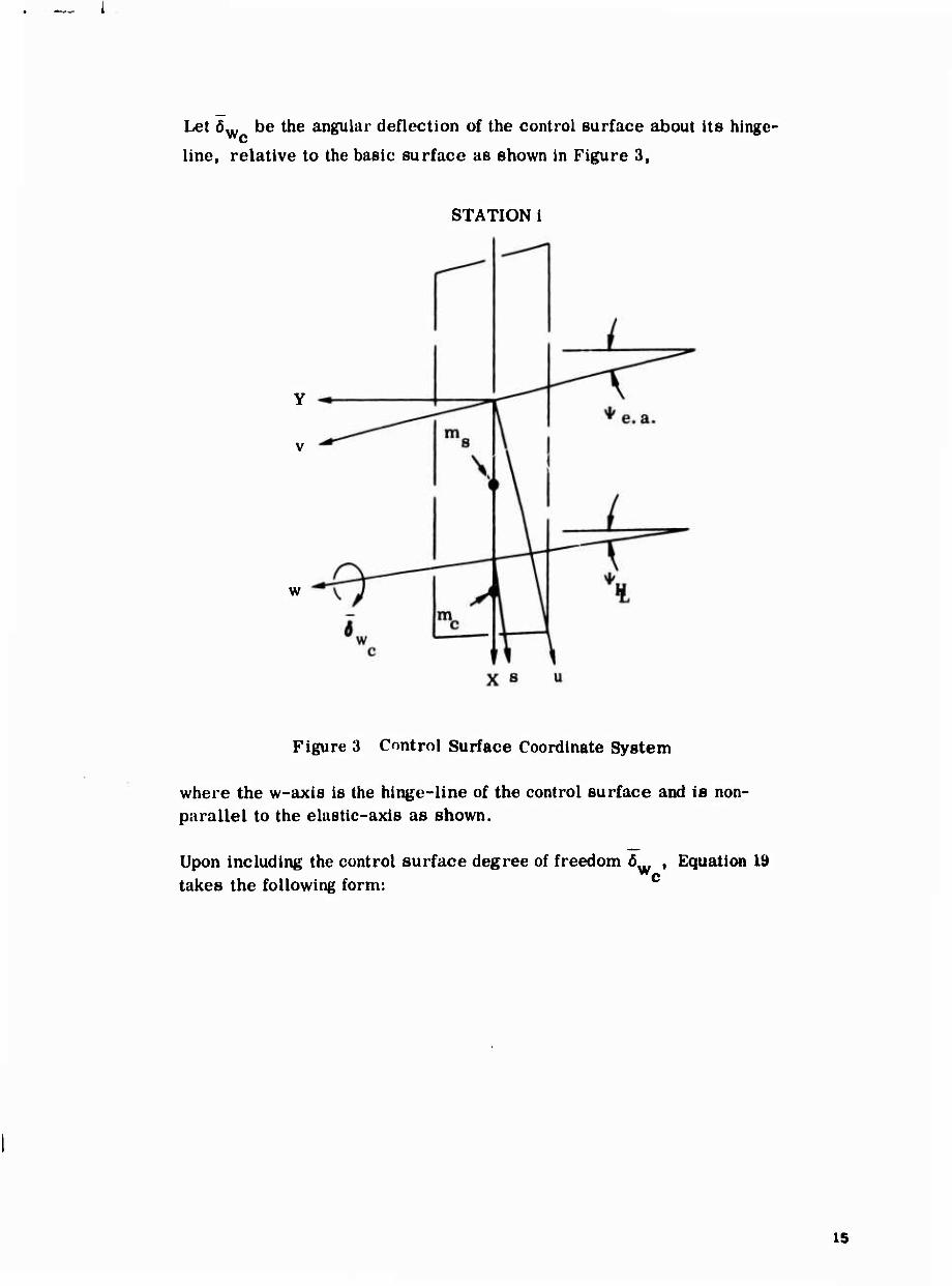
Let öw be the angular deflection of the control surface about its hinge-
line, relative to the basic surface as shown in Figure 3,
STATION i
w
Figure 3 Control Surface Coordinate System
where the w-axis is the hinge-line of the control surface and is non- parallel to the elastic-axis as shown.
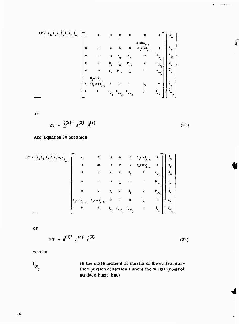
Upon including the control surface degree of freedom öw , Equation 19 takes the following form: c
15
2T-I « « ä Ä a ä « I L X Y / u v / w,.J
u 111
u 0
u u
0 0
S »In* u e. J .
Ü <S COB* v «-.a
Ü Ü
u u
in S
I »'
S Hilt» U t'.U.
*H CUB* v e.u.
U
U
0
w uw vw
*x 1 s 6
u
6 v |
K. w 1
c 1
or
2T = ö^' J(2) ö<2> (21)
And Equation 20 becomes
2T*[j 6 6 6 6 6 6 6 x y /, u v z -J u u
U Ü
m u
U I
0 S Hin* v f. a.
U S COB* v e.a.
u U S V
u V
0
iS Bill* v v u.
S CU8* v e.a
U Ü Ü '/.
1) Ü S w
c 1» uw
c p vw
c 0
u \
u \
i w
c 6
uw 1* "
vw t!
6 V
0 \
w c
w (
or
2T = ^' J{3) 6(2> (22)
where:
I w
is the mass moment of inertia of the control sur- face portion of section i about the w axis (control surface hinge-line)
16
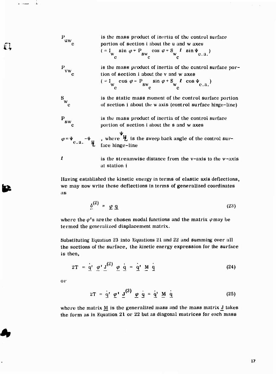
P is the mass product of inertia of the control surface uw
c portion of section i about the u and w axes ( = 1 sin üj-r P cos^-^S I sin* )
w sw w e. a. c c c
P is the mass product of inertia of the control surface por- vw
c tion of section i about the v and w axes ( = I cos (p - P sin </> + S i cos * )
w sw w e.a. c c c
S is the static mass moment of the control surface portion w
c of section i about the w axis (control surface hinge-line)
P is the mass product of inertia of the control surface sw
c portion of section i about the s and w axes
(/) = * -* , where ^L is the sweep back angle of the control sur- e.a. H
L tace hinge-line
I is the streamwise distance from the v-axis to the w-axis at station i
Having established the kinetic energy in terms of elastic axis deflections, we may now write these deflections in terms of generalized coordinates as
öy ' = (^q (23)
where the ^'s are the chosen modal functions and the matrix ^may be termed the generalized displacement matrix.
Substituting Equation 23 into Equations 21 and 22 and summing over all the sections of the surface, the kinetic energy expression for the surface is then,
(2) • • 2T = q' </>' J tf> q = q1 M q (24)
or
(3) • • 2T = q' ^, JV ' ^ q = q' M q (25)
where the matrix M is the generalized mass and the mass matrix J takes the form as in Equation 21 or 22 but as diagonal matrices for each mass
17
I „-iWlIfcW
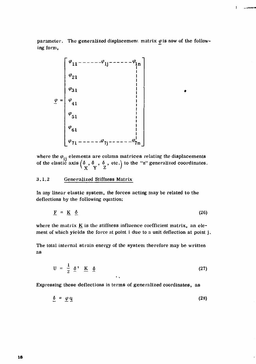
parameter. The generalized displacemem matrix (pis now of the follow- ing form,
<p =
<Pn ̂ v>ln
41
<P 51
^61
^71 J ^j ^7n
where the (p.. elements are column matrices relating the displacements of the elastic axis (ä , ö , Ö , etc.\ to the "n" generalized coordinates.
V X Y Z /
3.1.2 Generalized Stiffness Matrix
In any linear elastic system, the forces acting rnay be related to the deflections by the following equation;
K 6 (26)
where the matrix K is the stiffness influence coefficient matrix, an ele- ment of which yields the force at point i due to a unit deflection at point j,
The total internal strain energy of the system therefore may be written as
U = - ö1 K 6 (27)
Expressing these deflections in terms of generalized coordinates, as
Ö = (pq (28)
18
•...■•> k
and substituting into Equation 27, we obtain an expression for the inter- nal strain energy which is in terms of the generalized coordinates of the system:
= 1^3 (29)
where the matrix K is the generalized stiffness matrix.
Equation 1, Section 3.1, states that there is one Lagrange's equation of free undamped vibration for each generalized coordinate 0=1,2,3 — n).
Therefore, for the j1*1 coordinate,
d 37 au dt aq. 8q. ^j
J J
(30)
Applying Equation 30 to Equation 24, Paragraph 3.1.1, and Equation 29, Paragraph 3.1.2, results in the following: (For the generalized force Q equal to zero) J
I M.- M.0 — M. I L Jl j2 jnj
^o
\
L Jl j2 jnj
%
%
= 0
(31)
If we assume all coordinates except the j"1 equal to zero, the system moves in one coordinate and has a natural frequency appropriate to that coordinate. This is usually called the uncoupled frequency of the j4*1
coordinate.
Therefore, Equation 31 reduces to
M.. q. + Ks. q = 0 JJ J JJ J
(32)
If we assume harmonic motion in the system,
2 q. = -to. q.
J J J (33)
19
i MM—
Substituting Equation 33 into Equation 32,
2 -<*'. M,. q. + K.. q. = 0
J jj J JJ J 9
or
L2 M.. - K..^ \ J JJ JJ/ qj =0
(34)
Since q j^ 0,
KSi = to. M.. jj J JJ
(35)
And the generalized stiffness matrix K reduces to the following diagonal form:
K = 2
w, M.. j JJ
Equation 35 shows that zero elastic coupling exists between the coordi- nates as is the case with uncoupled or orthogonal modes.
3.1.3 Generalized Aerodynamic Matrix
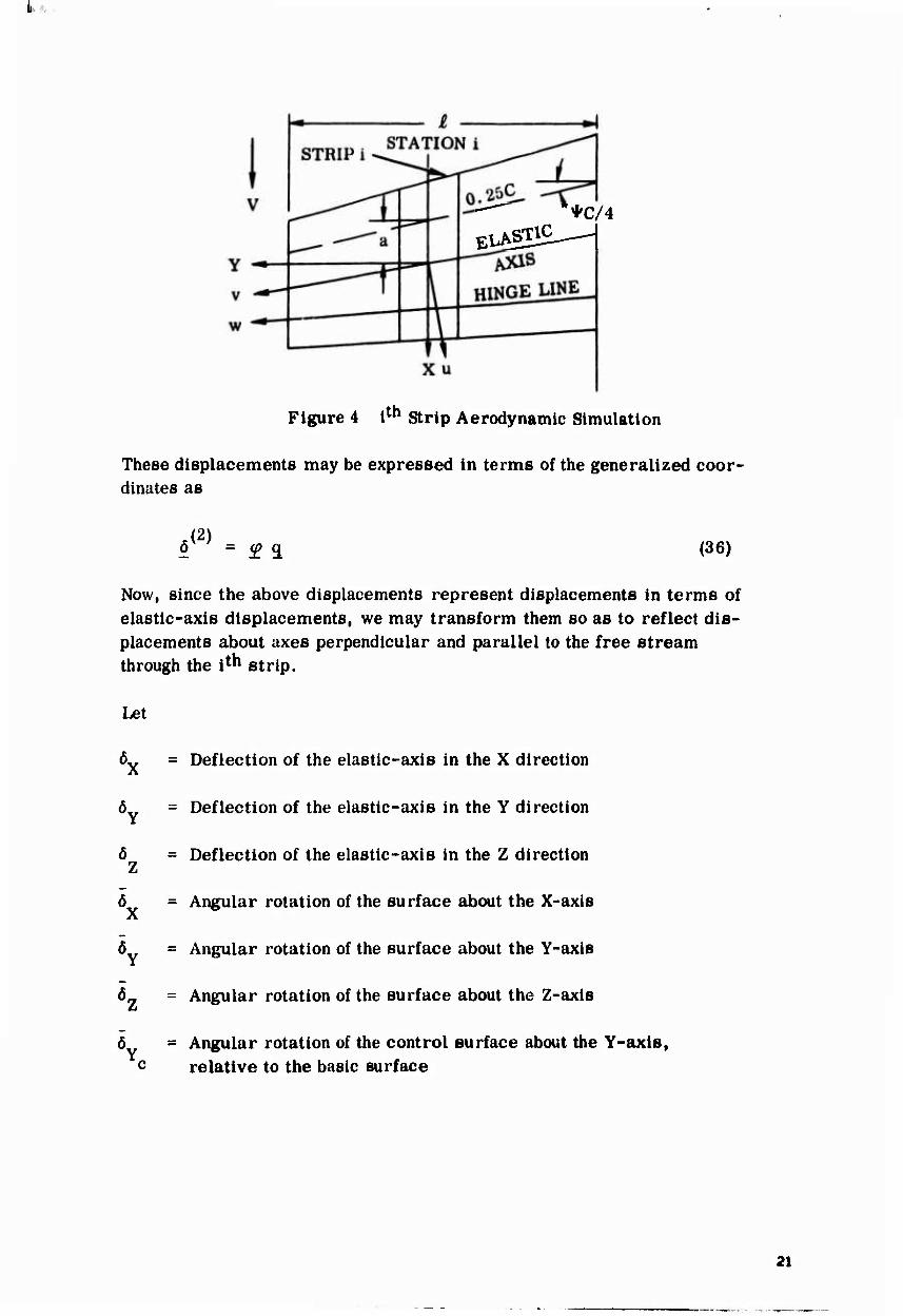
Consider the following displacements of the i strip shown in Figure 4 which represents a streamwise portion of the lifting surface as shown:
X = Deflection of the elastic-axis in the X-direction
= Deflection of the elastic-axis in the Y-direction
= Deflection of the elastic-axis in the Z-direction
u = Angular rotation of the surface about the u-axis
= Angular rotation of the surface about the v-axis
= Angular rotation of the surface about the Z-axis
w Angular rotation of the control surface about the w-axis, relative to the basic surface A
20
*C/4 EINSTIG,
AXIS
HINGEUNE-
Figure 4 Ith Strip Aerodynamic Simulation
These displacements may be expressed In terms of the generalized coor- dinates as
a<2> = e a (36)
Now, since the above displacements represent displacements in terms of elastic-axis displacements, we may transform them so as to reflect dis- placements about axes perpendicular and parallel to the free stream through the l**1 strip.
Let
= Deflection of the elastic-axis in the X direction
= Deflection of the elastic-axis in the Y direction
= Deflection of the elastic-axis in the Z direction
= Angular rotation of the surface about the X-axis
= Angular rotation of the surface about the Y-axls
Ö = Angular rotation of the surface about the Z-axls
Angular rotation of the control surface about the Y-axls, relative to the basic surface
Y
21
I -•*. t 'M
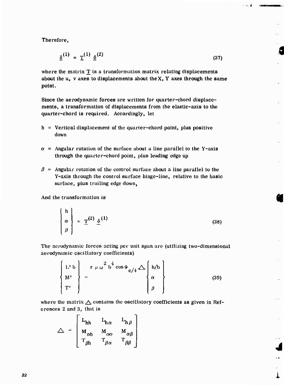
Therefore,
ö^1) = T(1) 6(2) (37)
where the matrix T is a transformation matrix relating displacements about the u, v axes to displacements about theX, Y axes through the same point.
Since the aerodynamic forces are written for quarter-chord displace- ments, a transformation of displacements from the elastic-axis to the quarter-chord is required. Accordingly, let
h = Vertical displacement of the quarter-chord point, plus positive down
a = Angular rotation of the surface about a line parallel to the Y-axis through the quarter-chord point, plus leading edge up
ß = Angular rotation of the control surface about a line parallel to the Y-axis through the control surface hinge-line, relative to the basic surface, plus trailing edge down,
And the transformation is
h
ß
T<2> öW (38)
The aerodynamic forces acting per unit span are (utilizing two-dimensional aerodynamic oscillatory coefficients)
(39)
f
L» b 2 4
n i) oo b cos * /, TV c/4
h/b
| M' ► =: i a
T1 ß
where the matrix TV contains the oscillatory coefficients as given in Ref- erences 2 and 3, that is
yv -
Lhh Sa Lhß
ah oo aß T T T lßh lßa ßß
22
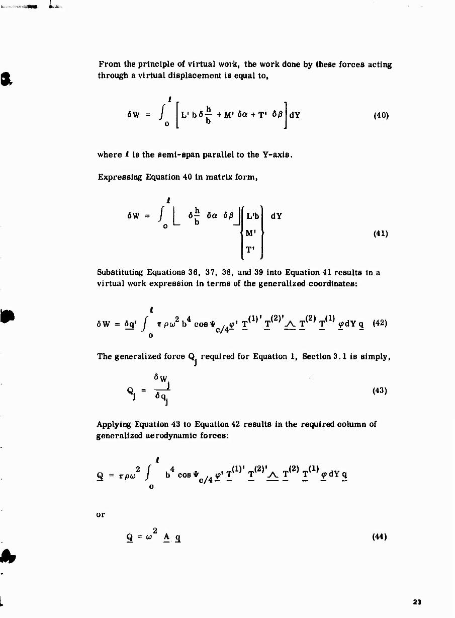
From the principle of virtual work, the work done by these forces acting through a virtual displacement is equal to,
ÖW = / L'bö- +1^ 6a + T ö/J b
dY (40)
where i is the semi-span parallel to the Y-axis.
Expressing Equation 40 in matrix form.
ÖW = / I ö^ öa öß\ L'b
M'
dY
(41)
Substituting Equations 36, 37, 38, and 39 into Equation 41 results in a virtual work expression in terms of the generalized coordinates:
ÖW = 63' / 7rpco2b4cos* ,4<g' T^'T^'-A. T(2) T(1) HY q (42)
The generalized force Q required for Equation 1, Section 3.1 is simply.
W.
Q. = J «q
(43)
J
Applying Equation 43 to Equation 42 results in the required column of generalized aerodynamic forces:
2 f K4 „,« * „. T^^' T^^ A T<2) T(1) «, dY a Q = Trpw J b cos* /AV *■ T -A. ^ T «iPclYq
or
Q = co A £ (44)
23
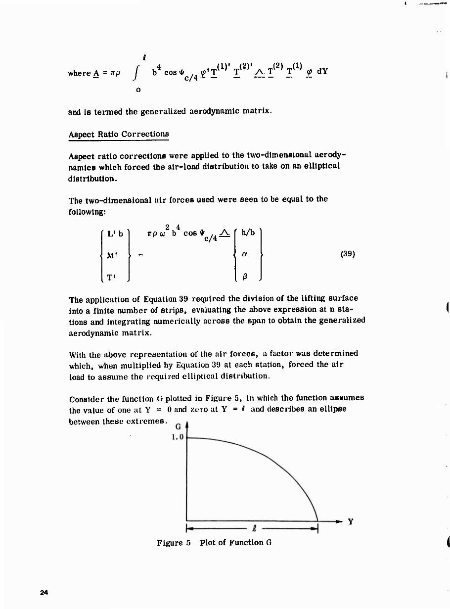
whereA = 7rp J b4 cos *c/4 ^'T(1), T^^^ T(2) T(1) ^ dY
i .-.
and is termed the generalized aerodynamic matrix.
Aspect Ratio Corrections
Aspect ratio corrections were applied to the two-dimensional aerody- namics which forced the air-load distribution to take on an elliptical distribution.
The two-dimensional air forces used were seen to be equal to the following:
fL'bl 2 4
TTO w b cos * /. jA; c/4
f h/b ]
a
ß J
(39)
The application of Equation 39 required the division of the lifting surface into a finite number of strips, evaluating the above expression at n sta- tions and integrating numerically across the span to obtain the generalized aerodynamic matrix.
With the above representation of the air forces, a factor was determined which, when multiplied by Equation 39 at each station, forced the air load to assume the required elliptical distribution.
Consider the function G plotted in Figure 5, in which the function assumes the value of one at Y = 0 and zero at Y = i and describes an ellipse between these extremes.
•► Y
Figure 5 Plot of Function G
24
*
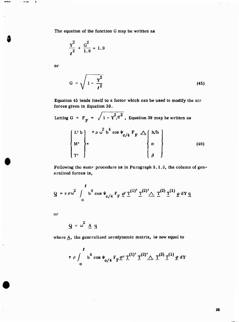
The equation of the function G may be written as
2 2 ^ + ^- = 1.0 i2 10
or
G = A/ 1- Ar (45)
Equation 45 lends itself to a factor which can be used to modify the air forces given in Equation 39.
Letting G = F
fL'b
-JV. .2^2
T« J
Y /^ , Equation 39 may be written as
f h/b 2 4
TT p w b cos * ,„ F„ .A. c/4 F —
a
[ ß J
(46)
Following the samr procedure as in Paragraph 3.1.3, the column of gen- eralized forces is,
d)'J2)'. J2)(l) q=itpw j b cos* , F ^»r ' r ;y\. r ;r'^dYq
or
2 Q = w A q
where A, the generalized aerodynamic matrix, is now equal to
n p f b4 cos * ., F tf' T^^ T^'^ T(2) T(1) tf dY J c/4 F— — — — •l-
26
i .~~m*
3.2 SYMMETRIC FLUTTER ANALYSIS
Study of the flutter characteristics of the empennage, symmetric sense, was initially restricted to an investigation of the basic horizontal stabili- zer with an assumed cantilevered restraint at the horizontal stabilizer pivot. Subsequent coupling of the stabilizer with the fuselage allowed an investigation into this added effect.
3.2.1 Cantilevered Analysis
The constrained empennage coordinates are the appropriate normal vibra- tion modes of the horizontal stabilizer consistent with the assumed canti- levered restraint. Therefore, the following generalized coordinates are considered:
q - Horizontal stabilizer rigid body pitch (about pitch axis)
q^ - Elevator rotation
q. - 1st coupled horizontal stabilizer elastic mode
q - 2nd coupled horizontal stabilizer elastic mode
q_ - 3rd coupled horizontal stabilizer elastic mode 5
3.2.1.1 Generalized Mass Matrix
Since only the horizontal tail is involved, the total generalized mass matrix is:
* - ^H.T.
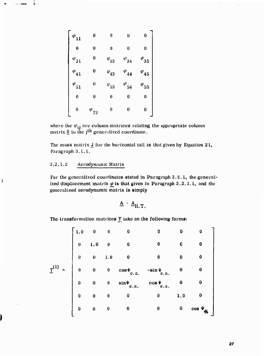
For the generalized coordinates given in Paragraph 3.2.1, the generalized displacement matrix for the horizontal tail takes the following form for the displacements indicated in Equation 21, Paragraph 3.1.1:
%
26
</>
</>
<p
<p
0 0 0 11
0 0 0 0 0
31 0
^33 ^34 ^35
41 0
^43 ^44 "45
51 U
^53 ^54 *55
0 0 0 0 0
0 Y72 0 0 0
where the ^y are column matrices relating the appropriate column matrix ö to the j1^ generalized coordinate.
The mass matrix J^ for the horizontal tail is that given by Equation 21, Paragraph 3.1.1.
3.2.1.2 Aerodynamic Matrix
For the generalized coordinates stated in Paragraph 3.2.1, the general- ized displacement matrix jp is that given in Paragraph 3.2.1.1, and the generalized aerodynamic matrix is simply
— -H.T.
The transformation matrices T take on the following forms:
,(1) _
1.0 0 0
0 1.0 0
0 1.0
0 0 0 cos* -sin* e.a. e.a.
0 0 0 sin*
L
0 0
0 o
e.a.
0
cos*
0
0
0 e.a.
0 1.0
0
0
0
0
0
0
0 cos * «.
27
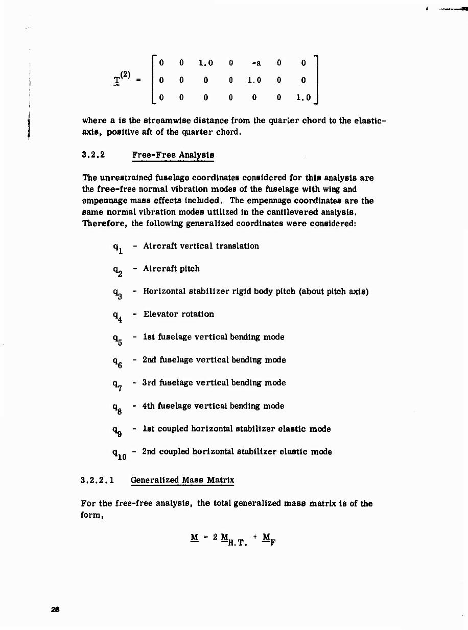
0 0 1.0 0 -a 0 0
T(2) = 0 0 0 0 1.0 0 0
0 0 0 0 0 0 1.0
where a is the streamwise distance from the quarler chord to the elastic- axis, positive aft of the quarter chord.
3.2.2 Free-Free Analysts
The unrestrained fuselage coordinates considered for this analysis are the free-free normal vibration modes of the fuselage with wing and empennage mass effects included. The empennage coordinates are the same normal vibration modes utilized in the cantilevered analysis. Therefore, the following generalized coordinates were considered:
q - Aircraft vertical translation
q^ - Aircraft pitch
a - Horizontal stabilizer rigid body pitch (about pitch axis)
q - Elevator rotation
q_ - 1st fuselage vertical bending mode 5
q - 2nd fuselage vertical bending mode 6
q - 3rd fuselage vertical bending mode
q - 4th fuselage vertical bending mode 8
qu - 1st coupled horizontal stabilizer elastic mode
q - 2nd coupled horizontal stabilizer elastic mode
3.2.2.1 Generalized Mass Matrix
For the free-free analysis, the total generalized mass matrix is of the form,
M = 2 MfI m + M^ — -H.T. —F
28
where the wing mass and mass-inertia effects are included as lumped elements in the fuselage mass distribution.
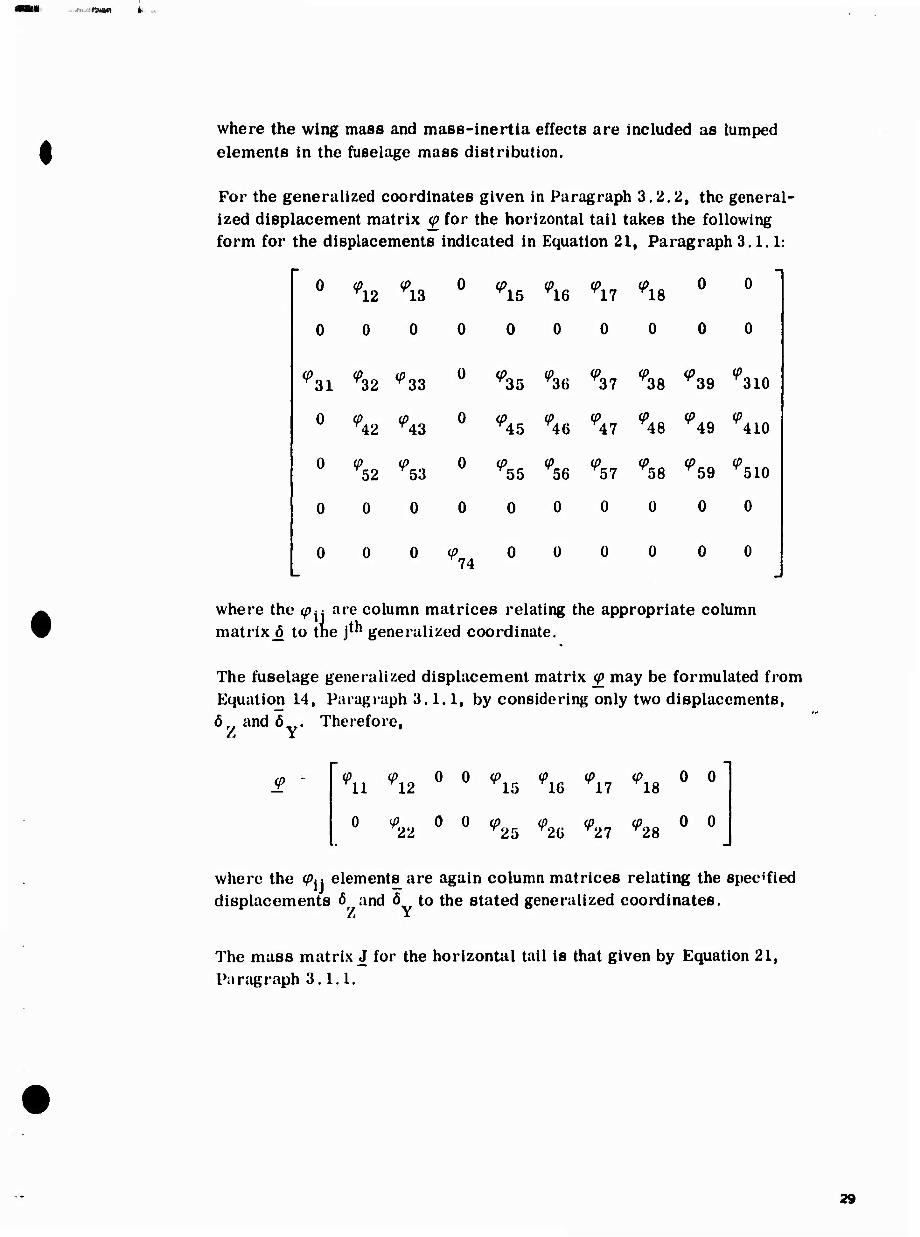
For the generalized coordinates given in Paragraph 3.2.2, the general- ized displacement matrix (p for the horizontal tail takes the following form for the displacements indicated in Equation 21, Paragraph 3.1.1:
0 0 (P 0 ^12 13
0 0 0 0
^31 ^32 ^33 0
0 ^42 ^3
0
0
0
%2
0
^53
0
0
0
0 0 0 (P 74
^IS ^16 ^17 ^18
0 0 0
0 0
Cl 0 0
(p 0 (O 0 0 0 ^35 ^36 37 38 39 310
0 0 0 0 0 0 M5 ^46 47 48 49 410
^55 ^56 ^57 ^58 ^59 ^510
0 0 0 0 0
0 0 0 0 0 0
where the 0^ are column matrices relating the appropriate column matrix^ to tne jt" generalized coordinate.
The fuselage generalized displacement matrix 0 may be formulated from Equation 14, Paragraph 3.1.1, by considering only two displacements,
Ö and Ö . Therefore, A Y
<P 0 0 0 0 0 0 0 0 00 Yn Y12 ^15 16 ^17 r18
0 0 0 0 0 0 0 0 00 22 25 T2(j T27 x28
where the 0,1 elements are again column matrices relating the specified displacements Ö and ö to the stated generalized coordinates.
The mass matrix J for the horizontal tail is that given by Equation 21, Paragraph 3.1.1.
29
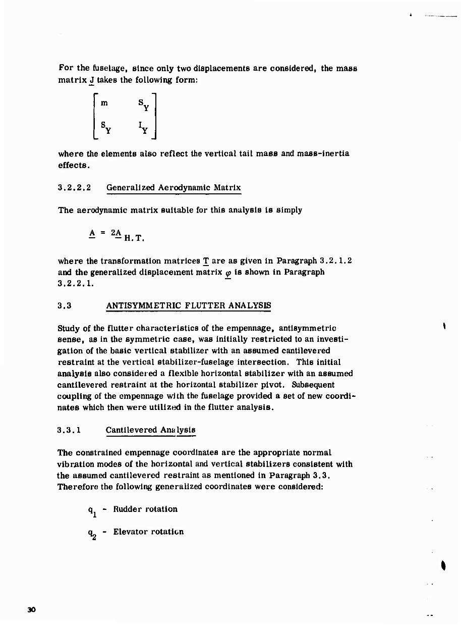
For the fuselage, since only two displacements are considered, the mass matrix J takes the following form:
m SY
SY 'Y
where the elements also reflect the vertical tail mass and mass-inertia effects.
3.2.2.2 Generalized Aerodynamic Matrix
The aerodynamic matrix suitable for this analysis is simply
^2^H.T.
where the transformation matrices T are as given in Paragraph 3.2.1.2 and the generalized displacement matrix y is shown in Paragraph 3.2.2.1.
3.3 ANTISYMMETRIC FLUTTER ANALYSIS
Study of the flutter characteristics of the empennage, antisymmetric sense, as in the symmetric case, was initially restricted to an investi- gation of the basic vertical stabilizer with an assumed cantilevered restraint at the vertical stabilizer-fuselage intersection. This initial analysis also considered a flexible horizontal stabilizer with an assumed cantilevered restraint at the horizontal stabilizer pivot. Subsequent coupling of the empennage with the fuselage provided a set of new coordi- nates which then were utilized in the flutter analysis.
3.3.1 Cantilevered Analysis
The constrained empennage coordinates are the appropriate normal vlbmtion modes of the horizontal and vertical stabilizers consistent with the assumed cantilevered restraint as mentioned in Paragraph 3.3. Therefore the following generalized coordinates were considered:
q - Rudder rotation
"h - Elevator rotation
%
30
<U - Horizontal stabilizer rigid body flapping
q - Horizontal stabilizer rigid body yawing
- 1st coupled horizontal stabilizer elastic mode
»6 - 2nd coupled horizontal stabilizer elastic mode
- 3rd coupled horizontal stabilizer elastic mode
q - 1st coupled vertical stabilizer elastic mode
q
- 2nd coupled vertical stabilizer elastic mode
10 - 3rd coupled vertical stabilizer elastic mode
3.3.1.1 Generalized Mass Matrix
For this phase of the antisymmetric analysis, the generalized mass matrix is of the form,
M =2MH]T> +MV_T_
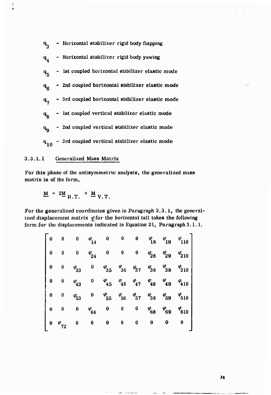
For the generalized coordinates given in Paragraph 3.3.1, the general- ized displacement matrix <£for the horizontal tail takes the following form for the displacements indicated in Equation 21, Paragraph 3.1.1.
0 0 0 r14 0 0 0
18 r19 U10
0 0 0 ^24
0 0 0 ^28 <P ^210
0 0 ^33
0 ^35 r36 ^37 ^S
<P 39 ^310
0 0 ^43
0 9 45 ^46 ^47 "48 "49 ^410
0 0 ^53
0 <P 55 ^56 ^57 % %
<P T510
0 0 0 ^64
0 0 0 ^68 ^69
<P 610
0 <p 0 0 0 0 0 0 0 0 72
M
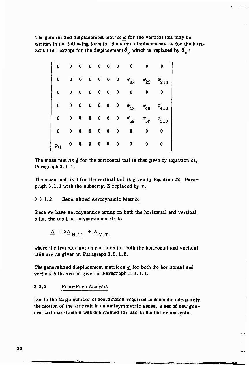
The generalized displacement matrix jg for the vertical tail may be written in the following form for the same displacements as for the hori- zontal tail except for the displacement 6 which is replaced by 6 :
0 0 0 0 0 0 0
o o o o o o o ^28 ^29 ^210
0 0 0 0 0 0 0 0 0
48 ^49 410
0 000000^.
0 0 0 0 0 0 0
58
0
5P 510
^71 0 0 0 0 0 0
The mass matrix J for the horizontal tail is that given by Equation 21, Paragraph 3.1.1.
The mass matrix J for the vertical tail is given by Equation 22, Para- graph 3.1.1 with the subscript Z replaced by Y.
3.3.1.2 Generalized Aerodynamic Matrix
Since we have aerodynamics acting on both the horizontal and vertical tails, the total aerodynamic matrix is
A = 2A „ „, + A „ „, — -H.T. -V.T.
where the transformation matrices for both the horizontal and vertical tails are as given in Paragraph 3.2.1.2.
The generalized displacement matrices £ for both the horizontal and vertical tails are as given in Paragraph 3.3.1.1.
3.3.2 Free-Free Analysis
Due to the large number of coordinates required to describe adequately the motion of the aircraft in an antisymmetric sense, a set of new gen- eralized coordinates was determined for use in the flutter analysis.
32
3.3.2.1 Modal Coupling
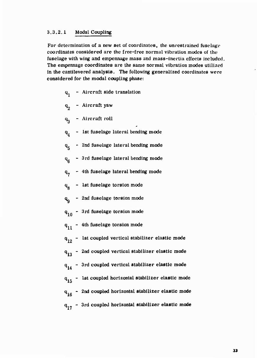
For determination of a new set of coordinates, the unrestrained fuselage coordinates considered are the free-free normal vibration modes of the fuselage with wing and empennage mass and mass-inertia effects included, The empennage coordinates are the same normal vibration modes utilized in the cantilevered analysis. The following generalized coordinates were considered for the modal coupling phase:
q - Aircraft side translation
q - Aircraft yaw
q - Aircraft roll
q - 1st fuselage lateral bending mode
q_ - 2nd fuselage lateral bending mode 5
q. - 3rd fuselage lateral bending mode o
q - 4th fuselage lateral bending mode
q - 1st fuselage torsion mode 8
\ - 2nd fuselage torsion mode
q - 3rd fuselage torsion mode
q - 4th fuselage torsion mode
q - 1st coupled vertical stabilizer elastic mode
q - 2nd coupled vertical stabilizer elastic mode
q - 3rd coupled vertical stabilizer elastic mode
q,. - 1st coupled horizontal stabilizer elastic mode 15
q - 2nd coupled horizontal stabilizer elastic mode
q - 3rd coupled horizontal stabilizer elastic mode
33
q - Rudder rotation lo
q - Elevator rotation
q - Horizontal stabilizer rigid body flapping all
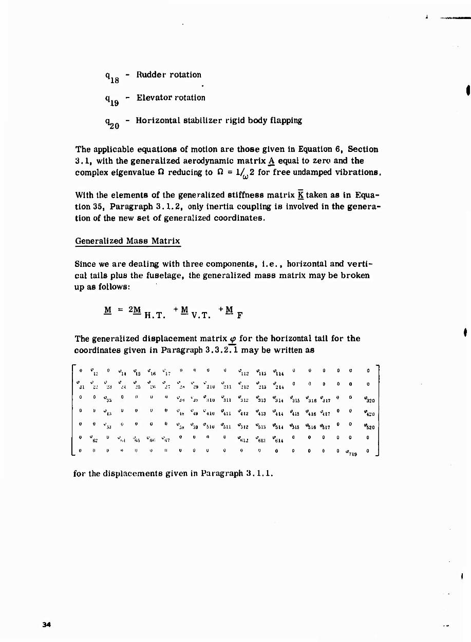
The applicable equations of motion are those given in Equation 6, Section 3.1, with the generalized aerodynamic matrix A equal to zero and the complex eigenvalue O reducing to ß = 1/2 for free undamped vibrations.
With the elements of the generalized stiffness matrix K taken as in Equa- tion 35, Paragraph 3.1.2, only inertia coupling is involved in the genera- tion of the new set of generalized coordinates.
Generalized Mass Matrix
Since we are dealing with three components, i.e., horizontal and verti- cal tails plus the fuselage, the generalized mass matrix may be broken up as follows:
M = 2MH.T. +MV.T. +MF
The generalized displacement matrix <p for the horizontal tail for the coordinates given in Paragraph 3.3.2.1 may be written as
0 U "u % If 16 ^17
u '1 u u iß 112 VU3 "U4
ü I) 0 0 0 0
,21 v» v1
IS 25 2i'< J>
in 29 "nu lj>
2\l if
212 ifi
2Vi ^214 0 0 0 0 0 Ü
0 0 "33
0 0 u I) ^1 % ;ilu *m ^312 313 ^314 315 316
If 317
0 0 0 320
0 u ^a u U u 0 *U
it 4» C41U "ui ^12 "413 **U "415 "416 "417
0 Ü "420
0 0 VV,3 u u Ü Ü if 0» "sio "511 "512 "513 *514 "515 ^16 ^17
u 0 "520
0 62
u "M "«3 V, -">:■
0 0 0 U "«12 "«U
0 614
0 0 0 0 0 0
0 0 () 11 n 0 o u 0 it. 719
for the displacements given in Paragraph 3.1.1.
34

For the vertical tail, the generalized displacement matrix y is
o o u 0 0 Ü U Ü U ü Ü u
*2l *22 ^23 ^4 ^28 ^2« ^27 V2« ^ ^210 ^ll V212 V213 ^214 0 0 Ü " 0 "
U ü 0 U ü ü 0 0 0 U U 0 o o
^42 43 44 45 46 ^47 48 4» 410 ^411 r4l2 ^413 V414
(ia>0ipit(p(p{fiW<p if <p if tfOOOOOü ^52 53 ^54 65 56 57 ^58 5» 510 ^511 ^512 ^513 ^514
0000000000
000000 OÜOO
0 0 0 0 0 0 0 0 0 0
0 0 0 0 0 0 0 r718 0 0
for the same displacements as for the horizontal tail except for the dis- placement 6 , which is replaced by Ö
The generalized matrix <p for the fuselage is
o o t» •17
0 § 20
U 0
^11 ^2 ^IS ^U ^IS ^16 ^17 ü
0 0 V^ 0 Q if tp ip ip 28 2» ^210 211
a <f <e if <e if ü TS2 0 ^34 35 36 ^37
00 0000 0 00
000000000 11
0 000000000
for only thrr' r nsidered displacements, 6 , Ö and 6 .
The mass matrix jJ for the horizontal tail is that given by Equation 21, Paragraph 3.1.1.
The mass matrix J for the vertical tail is given by Equation 22, Para- graph 3.1.1 with the subscript Z replaced by Y.
For the three displacements considered for the fuselage, the mass matrix J takes the following form:
m -S X
-s X
I X
0
0
0
where the elements also reflect the wing mass and mass-inertia effects.
35
3.3.2.2 Flutter Analysis
The new set of generalized coordinates determined from a solution of the equations of motion described in Paragraph 3.3.2.1, is as follows:
q - Aircraft side translation
q^ - Aircraft yaw
qu - Aircraft roll
q - Horizontal stabilizer rigid body yawing
q_ - Ist coupled fuselage - empennage elastic mode 5
q - 2nd coupled fuselage - empennage elabtic mode 6
q - 3rd coupled fuselap« - empennage elastic mode
q - 4th coupled fuselage - empennage elastic mode o
CL^ - 5th coupled fuselage - empennage elastic mode
q - 6th coupled fuselage - empennage elastic mode
Generalized Mass Matrix
As in the modal coupling phase, the generalized mass matrix may be split up into parts:
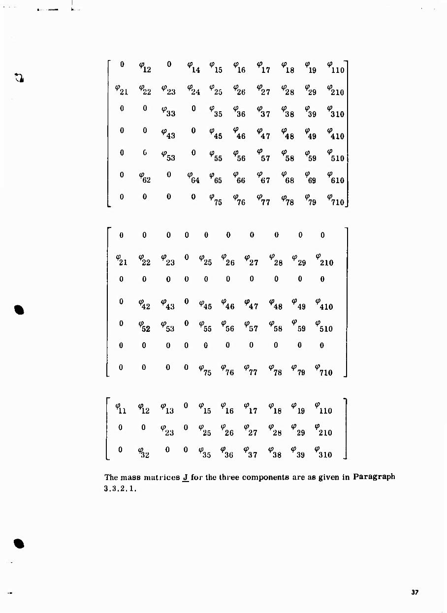
^=2^H.T. +^V.T. +^F
where the generalized displacement matrix <p for the horizontal tail, vertical tail and fuselage are, respectively,
36
k....
ti 0
^12 0
*14 "iS ^16 ^T 18 19 ^ 1 no
^21 </22 ^23 ^24 % (P V27
(P ^28 29
<P
0 0 ^33
0 *35
<P ^37 ^38 39 310
0 0 ^43
0 %
<P 46 ^47
V A8 ^49 9 410
0 G ^53
0 % ^56 57
<P 58 ^59 510
0 (p 0 ^64 <P 66 67 68 69 610
0 0 0 0 <P 75 r76 <P
77 ^78 <P 79 710j
0 ^42
0 ^52
0 0
0 0 0 0 0 0
(p(p(pO(p(P(p(P(p<P 21 r22 23 r25 26 r27 28 29 210
00 0000 0 0 00
VA'I 0 ^= ^« ^^ ^" ^ ^ 43 ^45 T46 T47 T48 49 410
r53 r55 56 ^57 58 59 510
0 0 0 0 0 0 0 0
0 0 OO0<P<P(P<P(P v u V15 r76 v77 v78 v79 r710
(P0<pO(p<P(P(p(p<P Ml ^19 M*» Tir; T1« T17 ^1H T 1Q 11 T12 T13 15 16 17 18 19 110
0 0(PO<P<P<p(p<P<P ^23 25 26 27 28 29 210
Oip 00<p<P<P(p<P<P r32 r35 36 37 38 39 310
The mass matrices J_ for the three components are as given in Paragraph 3.3.2.1.
37
Generalized Aerodynamic Matrix
As in the antisymmetric cantilevered analysis, the aerodynamic matrix may be written as
— -H.T. —V.T.
where the transformation matrices for both the horizontal and vertical tail are as given in Paragraph 3.2.1.2.
The generalized displacement matrix ^for both the horizontal and verti- cal tail are given under Generalized Mass Matrix.
38 I
4.0 DISCUSSION AND RESULTS
The presentation and discussion of the results of the empennage flutter analysis, in general, follows the sequence of Sections 3.2 and 3.3. Also, this section presents the idealization of the empennage used for the analysis, the structural properties of such structure, and other data required for the flutter analysis of the empennage.
4.1 IDEALIZATION OF AIRCRAFT
As previously mentioned, structural Idealization of the empennage and fuselage was restricted to equivalent beams possessing both flexure and torsional stiffness distributions, with the aerodynamic loading repre- sented by two-dimensional or strip-theory aerodynamic forces. Figure 6 of Reference 1 presents the actual structure of the XV-5A empennage and fuselage to be idealized.
4.1.1 Structural Representation
As the aircraft structure shown in Figure 6 of Reference 1 shows, this may be thought of as a number of components assembled to form the complete structure, i.e., fuselage and horizontal and vertical stabili- zers plus control surfaces. From this standpoint, the following para- graphs deal with these components as they were treated during the analysis.
4.1.1.1 Horizontal Stabilizer-Elevator
Figure 6 shows the planform of the horizontal stabilizer and elevator. The elastic-axis shown represents the equivalent beam which replaces the actual structure shown in Figure 6 of Reference 1. The elevator was taken as a rigid body having distributed mass and mass-inertia properties. The elevator system is manual; therefore, its rotational restraint was idealized into an equivalent spring. This, in conjunction with the pitching inertia of the elevator, resulted in an elevator rota- tional frequency, which was varied to cover expected ranges. Figure 8 presents a plot of the spanwise distribution of the bending and torsional stiffnesses for the horizontal stabilizer. These stiffness values reflect a maneuver flight condition, i. e., they reflect a mini- mum stiffness due to skin ineffectiveness.
39
4.1.1.2 Vertical Stabilizer-Rudder
Figure 7 shows the planform of the vertical stabilizer and rudder, with the elastic-axis shown representing the orientation of the equivalent beam which replaces the actual structure shown in Figure 6 of Reference 1. The rudder system, being equivalent to the elevator system, was idealized in the same fashion. Figure 9 presents a plot of the spanwise distributions of the bending and torsional stiffnesses for the vertical stabilizer. As for the horizontal stabilizer, these plots reflect a minimum stiffness, also.
4.1.1.3 Fuselage
The fuselage structure shown in Figure 6 of Reference 1 was idealized into an equivalent beam having vertical, lateral and torsional stiffness. These distributions are shown in Figure 10. The elastic axis of the fuselage was assumed to be at the intersection of the vertical plane at B. L. O with the horizontal plane at W. L. 113.00. With this represen- tation, the vertical stabilizer elastic-axis intersects the fuselage at F.S. 459.37, as shown in Figure 7.
4.1.2 Aerodynamic Representation
Since aerodynamic forces acting on the wing normally are small, com- pared to forces on the empennage when predominant empennage motion is involved, the wing contribution to the formulation of the aerodynamic matrix was neglected. Flutter analyses were performed for several different altitudes to observe effects of air density. The aerodynamic coefficients used reflected both incompressible and compressible flow. The former coefficients were based largely on the work of References 2 and 3, whereas the compressible coefficients were derived from those covered by References 4 and 5.
4.1.2.1 Empennage
Application of Equation 44, Paragraph 3.1.3, required the division of the horizontal and vertical tails into a number of spanwise strips oriented parallel to the free stream. Evaluation of Equation 44 at each of the air-force stations was then required, and the total aerodynamic matrix for the surface was formed by numerical integration. Figures 6 and 7 also depict the planforms which were used for generation of the aerodynamic matrix for the horizontal and vertical tails, respectively.
40
^/«MMM |i.«..
4.1.3 Mass Representation
Only one gross weight condition, thai ol the design gross weight of approximately 9200 lbs, was studied during the analysis. This weight condition was applied only to the free-free analysis, both symmetric and antisymmetric. From a given mass distribution, the distribution was reworked to reflect a lumped-parameter system which was governed by an axis system dictated by Equation 21 or 22 of Paragraph 3.1.1. Inconsistencies between distributions shown for the symmetric and antisymmetric analyses are attributed to the relative time between completion of each analysis with the consequent up-dating of a distri- bution.
4.1.3.1 Symmetric Analysis
The mass distribution of the two components, the horizontal tail and fuselage, required for both the initial cantilever analysis and the free- free analysis, are presented in Tables 1 and2 for the horizontal tail and fuselage, respectively. The properties shown reflect the nomenclature as described by Equation 21 of Paragraph 3.1.1. Elevator and elevator mass-balance are also shown separately to indicate the mass-balance distribution utilized in the analysis. Table 2 presents, in addition to the basic fuselage distribution, the wing and empennage mass proper- ties which made up the inertial force and moment contributions of these components to the fuselage symmetric normal modes.
4.1.3.2 Antisymmetric Analysis
The mass distribution of the three components, namely the horizontal tail, vertical tail and fuselage, required for both the initial cantilevered analysis and the free-free analysis, are presented in Tables 3 through 5 for the horizontal tail, vertical tail and fuselage, respectively. The properties shown again reflect the nomenclature as described by Equa- tion 21 of Paragraph 3.1.1. To show elevator and rudder mass-balance, separate tables of the balanced control surface and of the balance weights are also shown in Tables 3 and 4. Also shown in Table 4 are the hori- zontal tail mass properties which made up the inertial force and moment contribution of this component to the vertical stabilizer normal modes. Table 5 presents, in addition to the basic fuselage distribution, the wing and empennage mass properties which made up the Inertial force and moment contributions of these components to the fuselage antisymmetric normal modes.
41
4.2 MODAL FUNCTIONS
As mentioned in Section 3.0, the equations of motion were formulated in terms of modal functions. These were principally the normal modes of vibration of the component consistent with an assumed constraint.
4.2.1 Symmetric Analysis
As mentioned in Section 3.2, the components involved in the symmetric analysis were the horizontal stabilizer, fuselage and elevator. The horizontal stabilizer normal modes are the coupled modes (inertial) of bending and torsion of the equivalent beam considered cantilevered at the horizontal stabilizer pivot. The normal modes of the fuselage are the uncoupled free-free modes of the fuselage equivalent beam with wing and empennage mass and mass-inertia effects included. Vertical shear effects (AG) are also considered in the determination of these latter modes.
4.2.1.1 Cantilevered
Figures 11, 12 and 13 depict the first three cantilevered mode shapes of the horizontal stabilizer, while Table 6 gives a tabulation of the modal data. The vertical bending is denoted by (/'whereas the torsion of the surface about the elastic-axis is denoted by 9.
4.2.1.2 Free-Free
In addition to the horizontal stabilizer normal modes, the fuselage degrees of freedom were included, and these shapes are plotted in Figures 14 and 15, with the modal data tabulated in Table 7.
4.2.2 Antisymmetric Analysis
Also, as mentioned in Section 3.3, the components involved in the anti- symmetric analysis were the horizontal stabilizer, vertical stabilizer, and fuselage, plus elevator and rudder. The horizontal stabilizer nor- mal modes arc the coupled modes (inertial) of bending and torsion of the equivalent beam considered cantilevered at the horizontal stabilizer pivot. The vertical stabilizer normal modes are also the inertially coupled modes of bending and torsion of the equivalent beam considered cantil'vered at the intersection of the elastic-axis with the assumed fuselage clastic-axis (F.S. 459.37). Mass and mass-inertia effects of the horizontal tail were considered in these latter modes. The
42
normal modes of the fuselage are the uncoupled free-free modes of the fuselage equivalent beam, with wing and empennage mass and mass- inertia effects included.
4.2.2.1 Cantilevered
Figures 16, 17 and 18 present the first three cantilevered mode shapes of the horizontal stabilizer, while Table 8 tabulates the modal data. The equivalent information for the vertical stabilizer is presented in Figures 19, 20, and 21 and Table 9.
4.2.2.2 Free-Free
For the free-free analysis, as mentioned in Paragraph 3.3.2, coupled modes for the aircraft were calculated, and a new set of generalized coordinates was chosen for the flutter analysis. The horizontal and vertical stabilizer normal modes utilized in the coupling are the same constrained modes of vibration utilized in the cantilevered analysis. The fuselage mode shapes are presented in Figures 22 and 23 for the uncoupled lateral bending and in Figures 24 and 25 for uncoupled torsion, the modal data being shown in Table 10.
4,3 FLUTTER ANALYSIS
As explained previously, the analysis of the empennage has been divided into a symmetric and an antisymmetric investigation. Each of these analyses was then divided further into basic cantilevered analyses and then expended to allow for fuselage flexibility and aircraft rigid body degrees of freedom.
In general, most of the results of the flutter analyses are plotted in the conventional sense, i.e., overall damping (g) versus forward velocity (V). In addition, the flutter frequency (f) is also plotted versus velocity. Equation 6 of Section 3.1 implies that these will be n-r roots, where n is the number of generalized coordinates considered for the problem, and r is the number of generalized coordinates de- fining rigid body degrees of freedom of zero frequency. Since genera- tion of the air-force matrix A requires the selection of a reduced fre- quency parameter (k0), the curves of damping-frequency versus flutter speed were generated by considering a range of reduced frequency parameters. The flutter parameters were noted by recording the lowest velocity at which a V-g plot crossed the g = o axis and then noting the flutter frequency at this velocity from the V-f plot for the appropriate root.
43
4.3.1 Symmetrie
The initial phase of the symmetric analysis, as explained previously, was restricted to the basic horizontal tail, which was assumed canti- levered at the pivot. The next phase included fuselage effects and also aircraft rigid body degrees of freedom.
4.3.1.1 Cantllevered Analysis
The large number of parameters involved in the flutter analysis, such as elevator rotational frequency, horizontal tail pitch frequency, density, aerodynamic parameters (aspect-ratio corrections and effect of aero- dynamic balance) precluded an extensive variation of these parameters. Therefore, only those parameters which were felt to be significant were varied over a larger range. Both incompressible and compressible aerodynamic coefficients were used in this analysis, as the incompress- ible analysis indicated that a flutter problem existed on the basic horizontal tail.
Incompressible
Figures 26 through 30 present the results of the basic cantilevered analysis for a variable horizontal tail pitch frequency of 25 to 80 cycles per second, for a constant elevator rotational frequency of 10 cycles per second and at an altitude of sea-level. Aerodynamic parameters were such that aspect-ratio corrections and effects of aerodynamic balance were neglected.
Figures 31 through 33 present results equivalent to those in Figures 26 through 30, but for an elevator rotational frequency of 30 cps and for horizontal tail pitch frequencies of 40, 60 and 80 cps.
Figures 34 through 36 show the results of removing the elevator degree of freedom (assuming elevator to be rigidly clamped) from the analysis. Other parameters are as in Figures 31 through 33.
Figures 37 through 39 present effects of aspect-ratio corrections (tip-round-off) for variable horizontal tail pitch frequencies of 40, 60 and 80 cps, for an elevator rotational frequency of 10 cps, and at sea-level altitude.
Figure 40 shows the effect of including aerodynamic balance in the air- force matrix for a horizontal tail pitch frequency of 60 cps and an elevator rotational frequency of 10 cps, all at sea-level altitude.
Aerodynamic balance effects were accounted for by means of the method! described in References 2 and 3. These references treat any balance as external, (nose overhang exposed directly to the free stream), whereas the actual aerodynamic balance in the elevator is of an internal nature. It was felt that treatment of the balance effects by means of the techniques of References 2 and 3 would indicate trends, which would be sufficient for the analysis.
Figures 41 through 43 present altitude effects for a pitch frequency of 60 cps and an elevator rotational frequency of 10 cps. An altitude of 9300* represents the minimum altitude at which the maximum-limit dive Mach number is reached.
A cross-plot of horizontal tail pitch frequency versus flutter speed is presented in Figure 44 for the different parameteric studies shown in the V-g plots of Figures 26 through 43.
Compressible
Compressible flutter analyses, using aerodynamic coefficients for a Mach number of 0.60, 0.70 and 0.80, were conducted for a fixed horizontal tall pitch frequency of 60 cps and an elevator rotational fre- quency of 10 cps. Aerodynamic parameters (aspect-ratio corrections and effects of aerodynamic balance) were neglected for this phase of the analysis, with altitude variations taken for the four altitudes used in the incompressible analysis.
Figures 46 through 48 present the results for the sea-level condition, while the results for the 9300', 20,000« and 30,000' analyses are pre- sented in Figures 49 through 57. Only the roots of concern have been plotted on both the y-g and V-f plots.
The flutter speed deduced from the above figures represents an apparent speed and not a true flutter speed. This is because the speed corresponding to the particular Mach number, in general, is not equal to the apparent flutter speed. For this reason, an auxiliary plot is given in Figure 58, wherein the apparent flutter speeds deduced from Figures 46 through 57 have been converted to equivalent air speeds. Crossing of a particular altitude line with the plot generated from the apparent flutter speeds then yields a true flutter speed. Also included in Figure 58 are the incompressible results obtained from Figures 29 and 41 through 43.
45
4.3.1.2 Free-Free AnalyslB
The free-free analysis was conducted for two values of the elevator rotational frequency and for three values of the horizontal tail pitch frequency. The analysis was conducted for a sea-level condition with the aerodynamic parameter (aspect-ratio corrections and effects of aerodynamic balance) neglected. Figures 59 through 61 present the results of the analysis for an elevator rotational frequency of 10 cps, while the same equivalent results for an elevator rotational fre- quency of infinity (locked elevator) are presented in Figures 62 through 64, with a cross plot of the overall effects shown in Figure 65.
4.3.2 Antisymmetric
The initial phase of the antisymmetric analysis was restricted to the basic vertical tail, assumed cantilevered at the fuselage-vertical stabilizer intersection. This analysis included the effects of a flex- ible horizontal stabilizer. The second phase included fuselage effects and also aircraft rigid body degrees of freedom.
4.3.2.1 Cantilevered Analysis
As in the symmetric analysis, the large number of parameters in- cluded in the flutter analysis of the empennage, such as elevator and rudder rotational frequency, horizontal tail yawing and rolling, density, and aerodynamic parameters (aspect-ratio corrections and effect of aerodynamic balance) precluded an extensive variation of these para- meters. Therefore, only the parameters considered significant were varied. Only incompressible aerodynamic coefficients were used in this analysis, with aspect ratio effects and aerodynamic balancing effects ignored. The end-plating of the vertical tail by the tip-mounted, hori- zontal tail fully justified the use of the two-dimensional strip theory, while the neglect of the aerodynamic balance was felt to be of small concern in the overall analysis.
Figures 66 and 67 present the results of the cantilevered analysis of the empennage for a rigid body yawing frequency of 10 and 20 cps. As explained in Paragraph 4.3.2, the effects of a flexible horizontal stabilizer were included, in addition to the rigid body modes of flapping (rocking) and yawing. Antisymmetric motion of the elevators was included, with the frequency taken as 15 cps. Variations of the fre- quency of the latter mode, as shown in initial analyses not presented in this report, indicated no change in flutter mode or speed. Similar
1
I i
46
earlier studies of rudder frequency variations showed the same results; therefore, the rudder rotational frequency was held to 10 cps for the analysis. Horizontal tail flapping was held to 10 cps, which was felt to be reasonable for the large rolling moment of inertia involved. Studies of variations of this parameter in initial analyses also indicated no change in flutter speed or mode.
4.3.2.2 Free-Free Analysis
As explained in Paragraph 3.3. 2, because of the large number of coor- dinates required to define adequately the antisymmetric motion of the empennage, which would include effects of fuselage stiffness and also aircraft rigid body modes, it is a practical impossibility to vary all unknown parameters. Therefore, certain values of these parameters were fixed, based on initial analyses of the empennage assumed canti- levered from the fuselage. With this in mind, several analyses were performed for two values of the horizontal tail yawing frequency. All other structural parameters, such as rudder and elevator rotational frequency and horizontal tail flapping, were held to certain values in the modal coupling for the purpose of determining the set of new generalized coordinates required for the flutter analysis. As in the cantilevered analysis, only incompressible aerodynamic coefficients were used, with aspect ratio effects and aerodynamic balancing effects ignored.
Figures 68 and G9 present the results of the free-free antisymmetric analysis of the empennage for a horizontal tail yawing frequency of 10 and 20 cps, respectively. The parameters held fixed were rudder rotation of 10 cps, elevator rotation (assumed antisymmetric motion) of 15 cps, and a horizontal tail flapping frequency of 10 cps. The latter parameters were included in the modal coupling and were con- sequently reflected in the six antisymmetric fuse läge-empennage modes used as generalized coordinates for the flutter analysis.
47

•■^v ■5 ■, ■^•r
tt—«ii-^'» •■ I.
*
BLANK PAGE .4'i
sKi
.rs? «*■ -
5.0 CONCLUSIONS
Because of the manner in which the preliminary flutter analysis of the empennage was conducted, i.e., a breaking down into initial component analysis, conclusions may best be drawn based on the results presented in Section 4.0.
5.1 SYMMETRIC ANALYSIS - CANTILEVERED CONDITION
Figures 26 through 58 present the V-g plots of these analyses» in addition to cross-plots for over all evaluation. These initial analyses, preliminary in nature and done at a time when only parametric studies can be made, indicate (Figure 44) that the controlling parameter on the flutter speed of the horizontal tail is that of the horizontal tail rigid body pitch frequency.
Figure 58 presents the proposed flight boundary of the XV-5A aircraft; a 15% flutter margin on the limit dive speed at sea-level is 575 knots. The 15% requirement on V^ therefore necessitates a horizontal tail pitch frequency of approximately 55 cps, based on incompressible theory. The trend of the plots shown in Figure 44 shows that, as the pitch frequency is increased from a low value to the upper value, the flutter speed approaches the basic bending torsion flutter speed of the surface. The mode of flutter involved is that of horizontal tail pitch coupled with the first coupled elastic mode of the horizontal tail. The mode shapes of this mode are presented in Figure 11. It should be noted that this mode exhibits both a bending and torsion component, the shapes of which are characteristic of the first uncoupled bending and torsion modes of a cantilever beam. At 60 cps pitch frequency, the flutter frequency is 40 cps. Referring to Figure 29, the V-g plot for this condition shows that the 3rd root is the flutter mode. Tracing this plot back to zero airspeed, we find that the coupled mode of vibration is approximately 63 cps. Solution of the equations of motion for zero aerodynamics yields approximately the same results (65 cps). This result indicates a coupling between the pitch mode and the torsion component of the first coupled horizontal tail elastic mode. This effect is shown in Figure 45. Note that the frequencies of both the coupled and uncoupled elastic modes of the horizontal stabilizer are plotted against the results of coupling the elastic modes with a variable hori- zontal tail pitch frequency, for a constant elevator rotational frequency of 10 cps. From this plot, it can be seen that the mode of flutter of the horizontal tail would be dependent on the available horizontal tail
49
I
I pitch frequency. For a low value of pitch frequency the bending mode would predominate, whereas, for a higher value of pitch frequency, the torsion mode would be predominant. This effect is evident also In ^ ' Figures 26 through 39. _
Variations of the elevator rotational frequency of 10 ops, 30 cps, and finally locking out of the elevator (infinite restraint) showed no appreciable change in the flutter trends of the surface.
Changes in the aerodynamic parameters shown in Figure 44 also showed no appreciable change in the basic flutter trend.
Altitude trends are shown mainly to present the data. These indicate increasing flutter speeds, as is normal.
Compressible analyses were conducted, since the design flight envelope (see Figure 58) encompasses the high subsonic region and the initial incompressible analyses Indicated that a relatively high-pitch frequency was required. Figure 58 presents the results of these analyses for an assumed horizontal tail pitch frequency of 60 cps. The M = o results from Figure 29 and Figures 41 through 43 are also plotted. Th^ trend of the plots indicates the usual drop in flutter speed as the transonic region is approached. Crossing of a flutter plot for a particular altitude with the altitude line radiating from the origin yields only one or two true flutter speeds (extrapolated for the sea-level and 9300' altitude). The boundary defined by these points lies within the 15% margin on equivalent airspeed, which indicates that a possible flutter situation might exist on the XV-5A aircraft if the design flight envelope is to be met.
5.2 SYMMETRIC ANALYSIS - FREE-FHEE CONDITION
Figures 59 through G5 present the V-g plots of these analyses, along with a cross-plot for various elevator rotational frequencies, for three values of the horizontal tail pitch frequency. The lower boundary of Figure 65 (for an elevator frequency of 10 cps) is relatively insensitive to horizontal tail pitch frequency, whereas the upper boundary exhibits the same trend as for the cantllevered analysis (Figure 44). The flutter mode for the lower boundary is fuselage bending coupled with elevator rotation. However, raising the damping level by 0.03 (from g = o), eliminates this boundary, and the flutter mode is now in effect, essentially the same as shown for the cantllevered case. That is, the flutter mode is horizontal tail pitch coupled with predominant horizontal tail torsion for the higher pitch frequencies.
50
5.3 ANTISYMMETHIC ANALYSIS - CANTILEVEHED CONDITION
Figures 66 and 07 present the V-g plots of the Initial analysis of the empennage. Results indicate a stable system throughout the proposed flight envelope for anticipated yaw frequencies of 10 and 20 cps. Early preliminary analyses of the vertical tail with and without the effects of an elastic horizontal tail showed a low flutter speed which necessitated increasing the torsional stiffness of the vertical stabilizer. Figure 9 shows the increased tip stiffness resulting from this earlier study. The results shown in Figures G6 and 67 reflect this latter stiffness distribution.
5.4 ANTISYMMETHIC ANALYSIS - FREE-FREE CONDITION
Effects of fuselage elasticity and aircraft rigid body modes on the antisymmetric flutter characteristics of the empennage, as shown in Figures 08 and 09, indicate also a stable system throughout the design flight envelope of the XV-5A aircraft.
5.5 OVERALL EVALUATION
Basic trends shown by the preliminary empennage flutter analysis indicate possible existence of a flutter situation which is dependent upon establishment of the actual pitch frequency of the horizontal tail. The required pitch frequency is approximately 55 cps, based on the results of the symmetric cantilevered analysis. Compressible analy- ses indicate a required pitch frequency of somewhat greater than 55 cps; however, if one were to determine the required pitch frequency at a structural damping level of 0.03 (see Figures 59 through 61), the required frequency would be of the order of 55 cps. In all, the analy- ses presented in this report should be taken as a preliminary evalua- tion of the empennage. Subsequent analytical and experimental investi- gations should be directed toward finalization of the actual flutter characteristics of the XV-5A aircraft with due regard toward the findings presented in this report.
51

Tilt um$msmmi%MmmmvTmmm&&mmv%mmm}**
BLANK PAGE
6.0 APPENDIX
6.1 LIST OF REFERENCES
1. Report 163, "Preliminary Flutter'AnaljysljB.. Volume I- Wing, November, 1965.
2. Smilg, B. and Waaserman, L.S.: "Application of Three- Dimensional Flutter Theory to Aircraft Structures." Air Force Technical Report 4798, 1942.
3. Waaserman, L.S., Mykytow, W. J. and Spielberg* I.N.: "Tab Flutter Theory and Applications." Air Force Technical Report 5153, 1944.
4. No Author: "Tables of Aerodynamics Coefficients for an Oscillating Wing-Flap System in a Subsonic Compressible Flow." National Aeronautical Research Institute (N. L. L.) Report F.151, May, 1954.
5. Timman, R., Van de Vooren, A. I.:"Theory of the Oscillating Wing With Aerodynamically Balanced Control Surface in a Two-Dimensional, Subsonic, Compressible Flow." National Aeronautical Research Institute (N. L.L.) Report F.54, June, 1949.
53
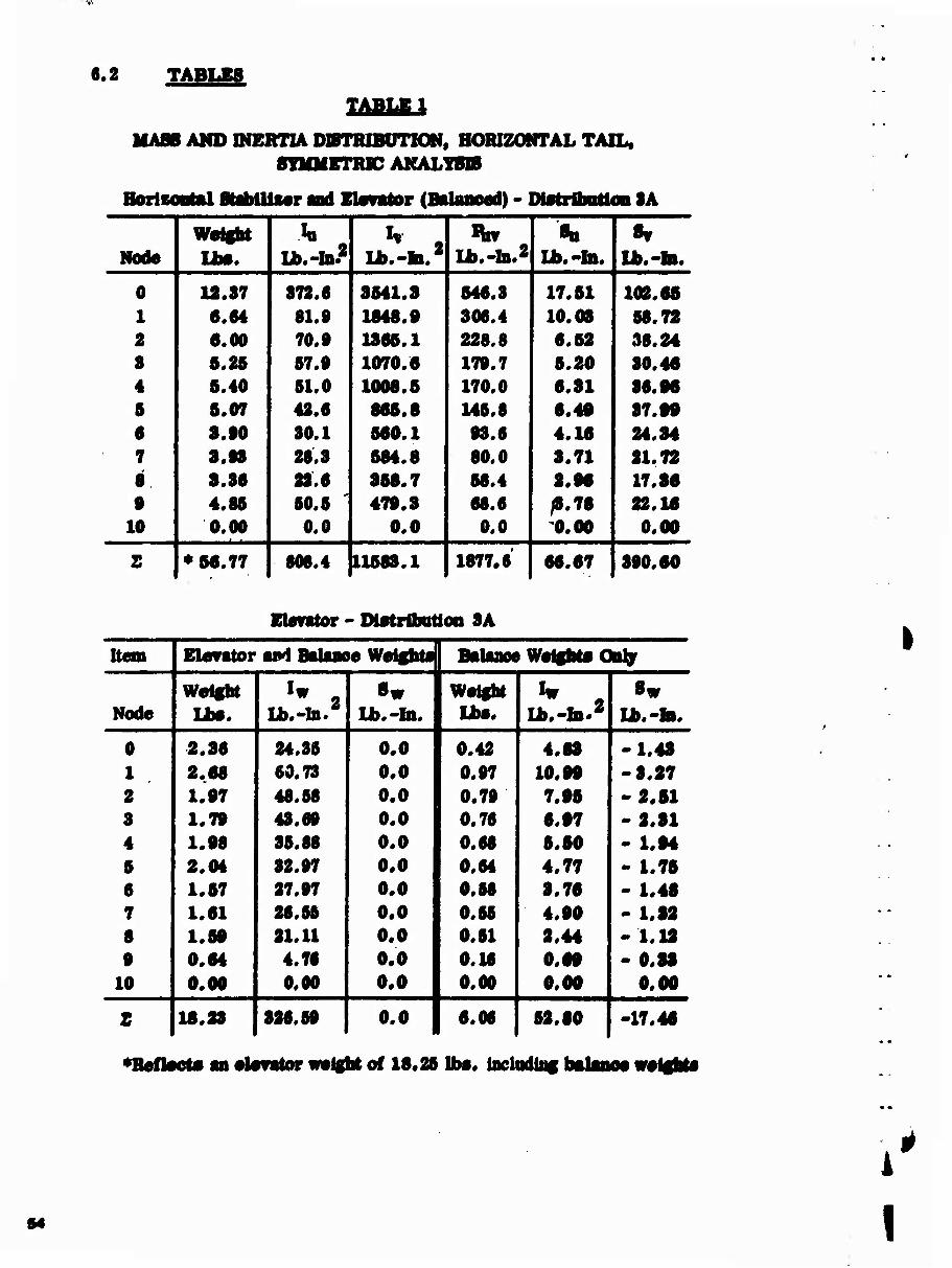
6.2 TABLES TABLE 1
MASS AMD INERTIA DBTRIBUT10II, HORIZONTAL TAIL, SYMMETRIC AKALYBD
HortBMtal StablllMr and Etomtor (Bftlaiioad) - ] DiotrlbiittonOA
Welfht 1 h 1 h 2 Lb.-to.
| Ikf 1 '8* ! ^ Node UM. U>.-lB.2 Ub.-b.2 Ui.-to. U.-to.
12.87 872.6 8541.8 546.8 17.51 102.65 6.64 81.0 1848.0 806.4 10.08 66.72
1 6'00 70.0 1866.1 228.8 | 6.52 38.24 5.26 67.0 1070.6 170.7 5.20 | 80.46 6.40 61.0 1008.5 170.0 6.81 86.06 6.07 42.6 865.8 | 146.6 6.40 87.00 8.00 80.1 860.1 08.6 4.16 24.84 8.08 | 26.8 584.8 80.0 8.71 21.72 8.86 22.6 858.7 58.4 2.06 17.86 4.86 1 60.6 1 470.8 | 66.6 /8.78 j 22.16
10 0.00 0.0 0.0 0.0 | 0.00 | 0.00
S ♦60.77 606.4 11588.1 1877.6 66.67 800.60
Elefttor • - DteiritmtlOD 8A
Ron Elerator airi Bftlaao* WeightiH Bolaaoe W«lghto Onljr
Weight lb.-In.
»w | 1 Weight 1 ^ 4 1 8w Node | Lbe. U>.-to. | UM. tb.-to.z Lb.-to.
2.86 24.36 0.0 1 o*42 4.88 -1.48 2.68 60.73 0.0 0.07 | 10.00 -8.27 1.07 48.68 0.0 0.70 { 7.05 - 2.51 1.70 48.00 0.0 0.76 0.07 - 2.81 1.08 | 86.68 0.0 0.68 6.50 | - 1.04 2.04 82.07 0.0 1 0«" 4.77 - 1.75 1.57 27.07 0.0 1 1 0'M 8.76 | - 1.46 1.61 26.66 o.o | i 0'M 4.00 | - 1.82 1.50 21.11 0.0 0.61 2.44 - 1.18 0.64 4.76 0.0 0.16 | 0.60 -0.88
10 | 0.00 0.00 0.0 1 o«00 1 0.00 0.00
Z 18.28 826.60 0.0 | 1 6'M 62.00 -17.46
I
♦Reflecte an eletator weight of 18.26 Ibe. indudiiig bftlaaoe weighto
i
1

4 8 in CM •-*
sJ 00 00 1 •-S ! M o © 1 © 1 Qd | • t* (N a
UM CM
1 3
H
^ ^ 1 ^
o C4c-tH^MCOMO>0><^00^0>ÄcOO
CM
^ ^ CO 1 ^
hfl ^ "* oao^C'.aoincoOoiot-'rHeo^t-^Ot^
HNQO0O©t*<Ot-O0NH C4
• 00
.H s iH N a> •
m o>
^ä 1 3 CM N 1 1 ''"^
1 »P^
•9 1 CSI • Oi o>
$ ^ «—< t* •> d 3 CO 1 CO
«^ ^ t 1 0) >
la • 00
• 00 1 »H ■H
iH i-l
*
(fi to
^d s 00
35 ^
1 CM • i-t i-t
^
t« t- •-4 CO 5 5
"3 CM
I3 • iH
•
iH iH
C4 • O O
5 S5 5H I <M CM
iJT . H fH
3 t- O CM
t- t-
Si V 1
CM •
CO t- «0
N i CM
1 O U)lOI>00iHC000 U> iH O O 00 t> «5 t-|
• •••••• •#•*•• • r-i
? « CO ifi
tä O 00 t- t- 00 Iß CO AQt>HC0^* «O l> oo 00 oo t- oo 05 co 0(0aoc40»^ CM i
t*
3 1 HNOOOOOt- t-Q0Nr-« (N g rH «O
1' O HMCO^lDtOt^aOOlOHCMCO^tAVt« PI
55
u-MH-«'-**"* *«■**-■■
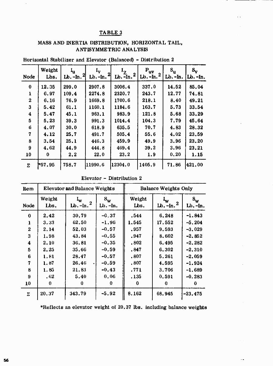
TABLE 3
MASS AND INERTIA DISTRIBUTION, HORIZONTAL TAIL, ANTISYMMETRIC ANALYSIS
Horizontal Stabilizer and Elevator (Balanced) - - Distributi on 2
Node Weight
Lbs. Lb.-In.2 Lb.-In.2 'Z 2 Lb.-In.2
p uv
Lb.-In.2 Su
Lb. -In. Sv
Lb.-In.
0 12.35 299.0 2907.8 3006.4 337.0 14.52 85.04 1 G.97 109.4 2274.8 2320.7 243.7 12.77 74.81 2 6.16 76.9 1669.8 1700.6 218.1 8.40 49.21 3 5.42 61.1 1160.1 1184.6 163.7 5.73 33.54 4 5.47 45.1 963.1 983.9 121.8 5.68 33.29 5 5.23 39.3 991.3 1014.4 104.3 7.79 45.64 6 4.07 30.0 618.9 635.5 70.7 4.83 28.32 7 4.12 25.7 491.7 505.4 55.6 4.02 23.59 8 3.54 25.1 446.3 459.9 49.9 3.96 23.20 9 4.62 44.9 444.8 469.4 39.2 3.96 23.21
10 0 2.2 22.0 23.2 1.9 0.20 1.15
2 *57.95 758.7 11990.6 12304.0 1405.9 71.86 421.00
Elevator - Distribution 2
Item Elevator and Balance Weights Balance Weights ( Only
Node Weight
Lbs. ^ 2 Lb.-In/ Sw
Lb. -In. Weight
Lbs. ^ 2 Lb.-In.2 Lb.-In.
0 2.42 30.79 -0.37 .544 6.248 -1.843 1 3.33 62.50 -1.96 1.545 17.552 -5.204 2 2.14 52.03 -0.57 .957 9.593 -3.029 3 1.98 43.84 -0.55 .947 8.602 -2.852 4 2.10 36.81 -0.35 .802 6.495 -2.282 5 2.25 35.66 -0.59 .847 6.302 -2.310 6 1.81 28.47 -0.57 .807 5.261 -2.059 7 1.87 26.46 • -0.59 .807 4.595 -1.924 8 1.85 21.83 -0.43 .771 3.706 -1.689 9 .62 5.40 0.00 .135 0.591 -0.283
10 0 0 0 0 0 0
2 20.37 343.79 -5.92 8.162 68.945 -23.475
♦Reflects an elevator weight of 20.37 lbs. including balance weights
56
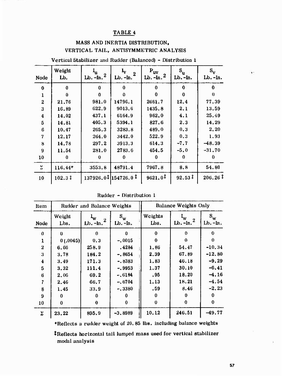
TABLE 4
MASS AND INERTIA DISTRIBUTION, VERTICAL TAIL, ANTISYMMETRIC ANALYSIS
Vertical Stabilizer and Rudder (Balanced) - Dis tribution 1
Node Weight
Lb. ^ 2 Lb.-In/ ^ 2
Lb. -In.
p UV O
Lb.-In.2 Su
Lb. -In. SV
Lb. -In.
0 0 0 0 0 0 0
1 0 0 0 0 0 0
2 21.76 981.0 14796.1 2661.7 12.4 77.39 3 16.89 622.9 9013.6 1435.8 2.1 13.59 4 14.02 437.1 6164.9 962.0 4.1 25.49 5 14.81 405.3 5394.1 827.6 2.3 14.29 6 10.47 265.3 3283.8 489.0 0.3 2.20 7 12.17 264.0 3442.0 522.9 0.3 1.93 8 14.78 297.2 3913.3 614.3 -7.7 -48.39 9 11.54 281.0 2783.6 454.5 -5.0 -31.70
10 0 0 0 0 0 0
V 116.44* 3553.8 48791.4 7967.8 8.8 54.80
10 102.3t 137926.0t 154726.0t 9621.0t 92.53t 206.26t
Rudder - Distribution 1
Item Rudder iiid Balance Weights | Balance Weights Only
Node Weight
Lbs. ^ 2
Lb.-In. Lb.-In. Weights
I Lbs. ^ 2 Lb.-In/ Lb.-In.
0 0 0 0 | 0 0 0
1 0(.Ü045) 0.3 -.0015 0 0 0 2 6.60 258. Ü .4284 ; | 1.86 54.47 -10.34 3 3.78 184.2 -. 8654 | 2.39 67.89 -12.80
4 3.49 171.3 -. 8383 1.83 46.18 -9.29 5 3.32 111.4 -.9953 j 1.37 30.10 -6.41 6 2.06 09.2 -.6184 .95 18.20 -4.16
7 2.46 66.7 -.6704 1.13 18.21 -4.54
8 1.45 33.9 -.3380 .59 8.46 -2.23
9 0 0 0 0 0 0
10 0 0 0 0 0 0
2 23.22 895.9 -3.8989 1 10.12 246.51 -49.77
♦Reflects a rudder weight of 20.
tReflects horizontal tail lumped modal analysis
85 lbs. including balance weights
mass used for vertical stabilizer
57
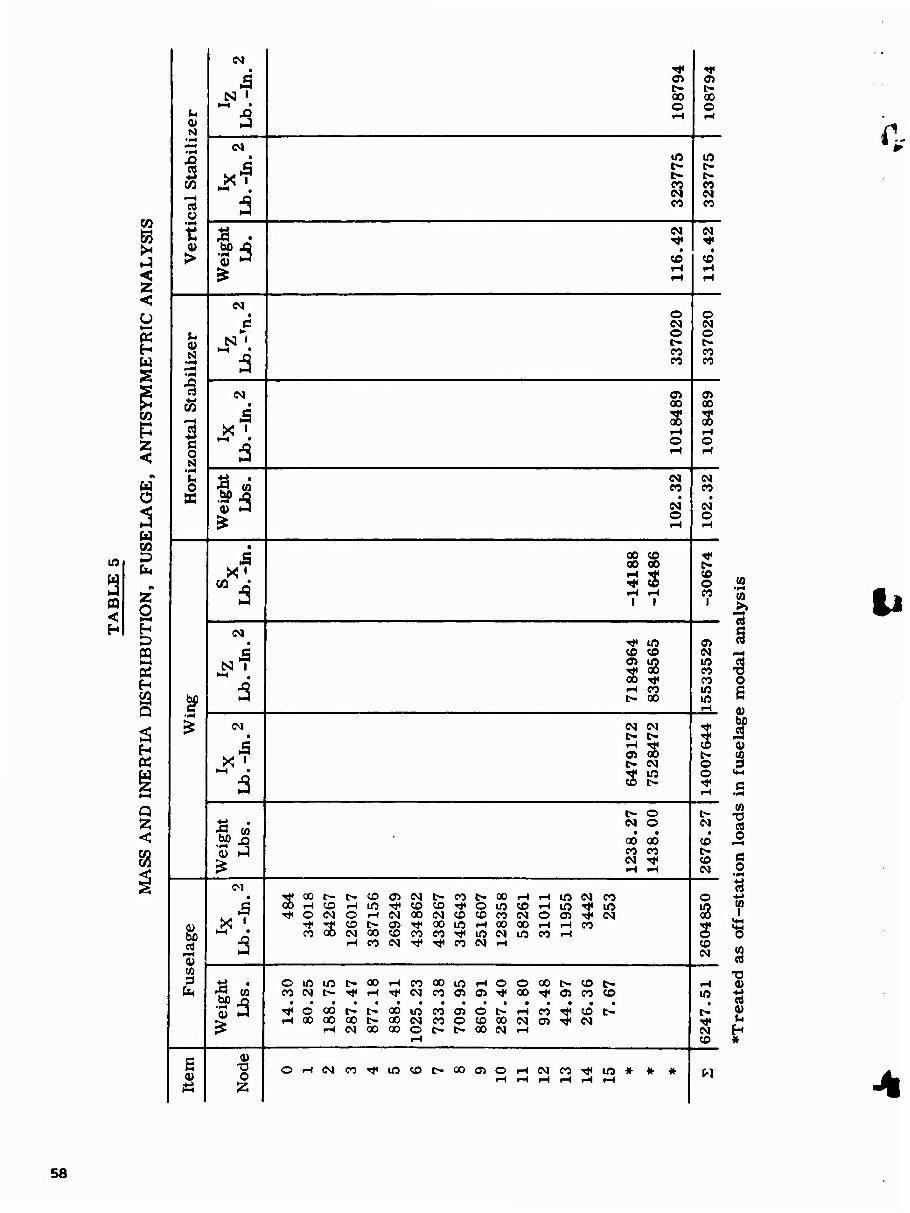
lO
ffl <
CO 53
<
< U i—
K H W
N
1 CO
1 <—<
t >
•
N • 00
H
(N
3 •> 1 s CO
l> t- co M CO
bfi jD 1 N
CO iH
1 ,H
• H H
N
'S
o
(N • e
a
o
fr" i CO
CO
O (N O
00 eo
• S
a
Oi 00
o
00
O H
0) »-3
CO • 1
! o
CO
o rH
•
wa -14
18
8
-16
48
6
(O o CO i
(N
a 7184
964
8348
565
IN ifi CO CO lO
i-H
IN • a
X '
a 6479
172
7528
472 i
o o rH
bß o
1238.2
7
14
38
.00
IN •
to
«0 IN
CO
1 ^
•
a
'*Q0t^t>CÖOiMt-COI>00fHiHinC^CO OOrHCOpHinr^^Cß^OlOCOr-tirj^lO Tt<0(NOiHMQO(NCO«OCONOOJ^<C<l
coob(NOOi©coeo^«inNirjcOfH fHcoMTf^eoNi-i
o s CO IN
OmiOI>Q0rHC000i0r-IOO00t*.?0|> CONt^^r-l^(NCOO»OS^OO-<tO»COCO
TfoQOt--t^ooiocoa>ot-iHcoTt<*oc- rHOOQOOOt-OOCOCOOCDOOMOi^M
i-(MQ000Ot>t>00MrH rH |
rH m •
CO
Item
1 o Ä 1
OrHCMW-^lOCOt-QOClOrHeOCO^UO* * * M
r.
(0
(0
i rH
o e
I co 3
CO
ei O
rH
ß o
? (0 cd
T3 (Ü
0) u H *
58
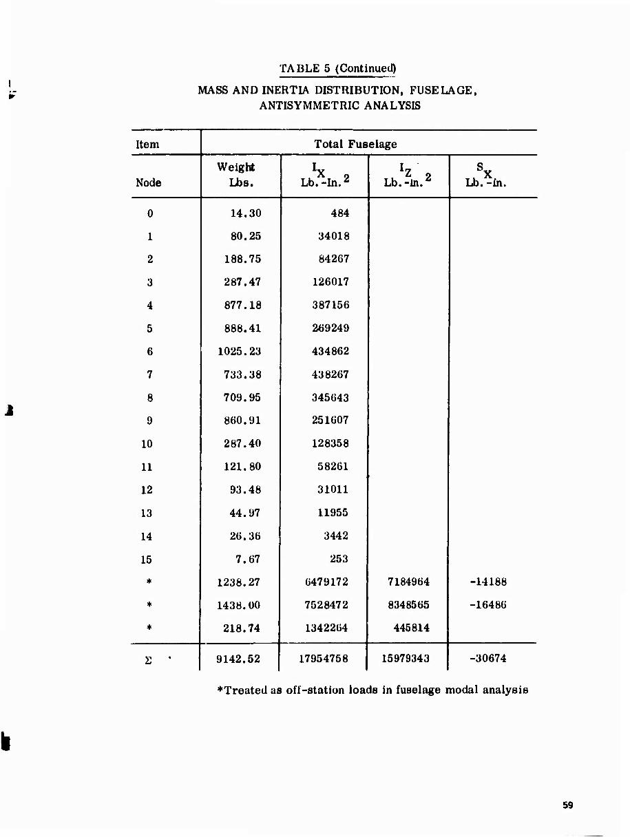
TABLE 5 (ContinueJ)
MASS AND INERTIA DISTRIBUTION, FUSELAGE, ANTISYMMETRIC ANALYSIS
Item Total Fuselage
Node Weight
Lbs. lX 2 Lb.-In.2 1 ^2 Lb.-ln.^ 1 A i Lb. -In.
0 14.30 484
1 80.25 34018
2 188.75 84267
3 287.47 126017
4 877.18 387156
5 888.41 269249
6 1025.23 434862
7 733.38 438267
8 709.95 345643
9 860.91 251607
10 287.40 128358
11 121.80 58261
12 93.48 31011
13 44.97 11955
14 20.36 3442
15 7.67 253
* 1238.27 6479172 7184964 -14188
♦ 1438.00 7528472 8348565 -16486
♦ 218.74 1342264 445814
2 ' 9142.52 17954758 15979343 i -30674
♦Treated as ofl-station loads in fuselage modal analysis
59
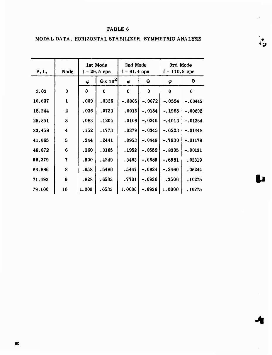
TABLE 6
MODAL DATA, HORIZONTAL STABILIZER, SYMMETRIC ANALYSIS *\
B.L. Node 1st Mode
f = 29.5 cps 2nd Mode
f = 91.4 cps 3rd Mode
f = 110.9 cps
0
V Gx 102
i ^ 6 <P e
3.03 0 0 0 0 0 0
10.637 1 .009 .0336 -.0005 -.0072 -.0524 -.00445
18.244 2 .036 .0733 .0015 -.0154 -.1965 -.00892
25.851 3 .083 .1204 .0108 -.0245 -.4013 -.01264
33.458 4 .152 .1773 .0379 -.0345 -.6223 -.01448
41.065 5 .244 .2441 .0953 -.0449 -.7930 -.01179
48.672 6 .360 .3185 .1952 -.0552 -. 8305 -.00131
56.279 7 .500 .4249 .3463 -.0685 -.6581 .02319
63.886 8 .658 .5486 .5447 -.0824 -. 2460 .06244
71.493 9 .828 .6533 .7701 -.0936 .3506 .10275
79.100 10 1.000 .6533 1.0000 -.0936 i
1.0000 .10275
60
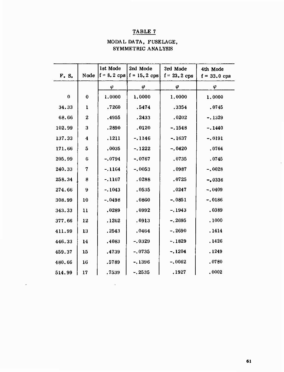
TABLE 7
MODAL DATA, FUSELAGE, SYMMETRIC ANALYSIS
1st Mode 2nd Mode 3rd Mode 4th Mode F. S. Node f = 8.2 cps f = 15.2 cps f = 23.2 cps f = 33.0 cps
0
<P <P <P 1 V 0 1.0000 1.0000 1.0000 1.0000
34.33 1 .7260 .5474 .3354 . 0745
68.66 2 .4955 .2433 . 0202 -.1329
102.99 3 .2890 .0120 -.1548 -.1440
137.33 4 .1211 -.1146 -.1637 -.0191
171.66 5 .0035 -.1222 -.0420 .0764
205.99 6 -.0794 -.0767 .0735 .0745
240.33 7 -.1164 -.0053 .0987 -.0028
258.34 8 -.1167 .0288 .0725 -.0336
274.66 9 -. 1043 .0535 .0247 -.0409
308.99 10 -.0498 .0860 -.0851 -.0186
343.33 11 .0289 .0992 -.1943 .0389
377.66 12 .1262 .0913 -.2695 .1000
411.99 13 .2543 . 0464 -.2690 .1414
446.33 14 .4083 -.0329 -.1829 .1426
459.37 15 .4739 -.0735 -.1204 .1249
480.66 16 .5789 -.1396 1 -.0062 ! .0780
514.99 17 .7539 1 -.2535 i .1927 i .0002
61
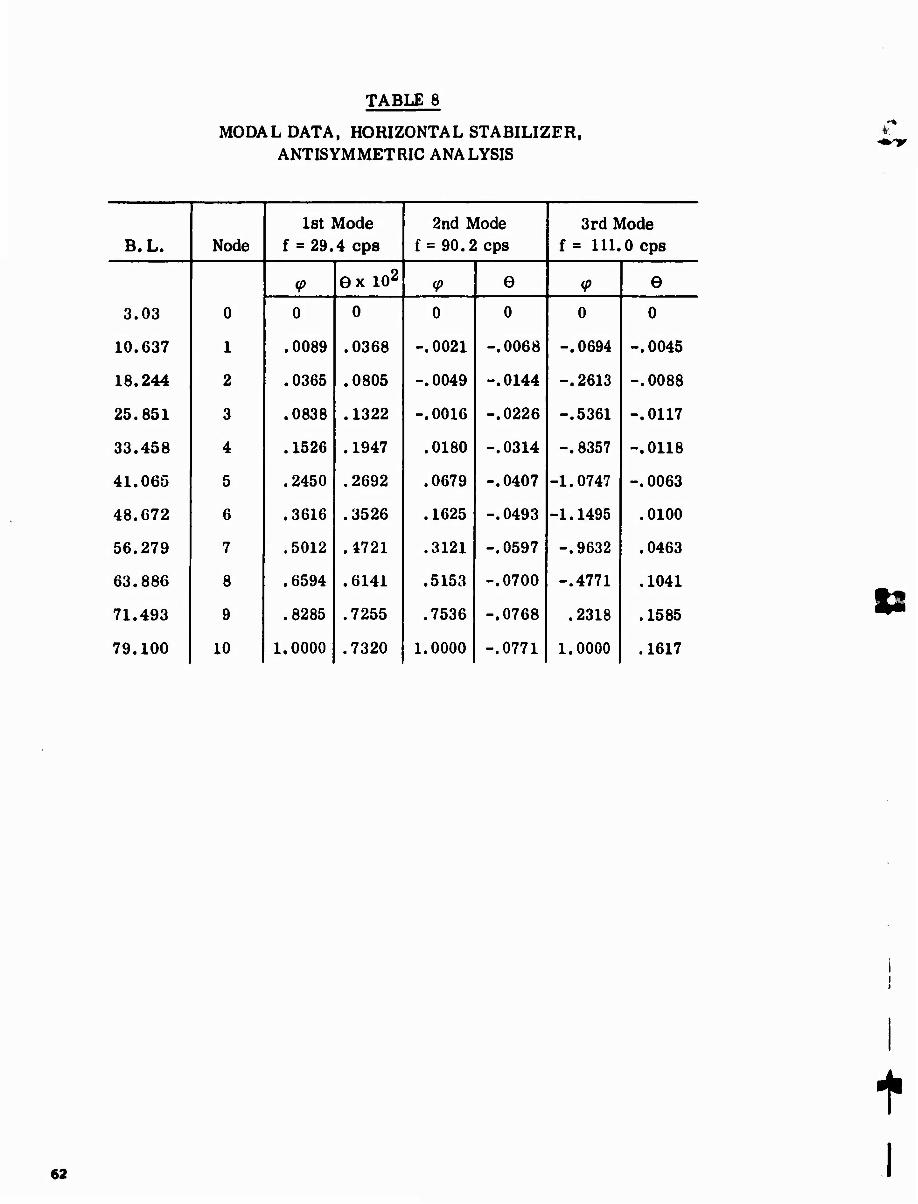
TABLE 8
MODAL DATA, HORIZONTAL STABILIZER, ANTISYMMETRIC ANALYSIS
B.L. Node 1st Mode
f = 29.4 cps 2nd Mode
f = 90.2 cps 3rd Mode
f = 111.0 cps
0
<P ex io2 <P e <P e
3.03 0 0 0 0 0 0
10.637 1 .0089 .0368 -.0021 -.0068 -.0694 -.0045
18.244 2 .0365 .0805 -.0049 -.0144 -.2613 -.0088
25.851 3 .0838 .1322 -.0016 -.0226 -.5361 -.0117
33.458 4 .1526 .1947 .0180 -.0314 -.8357 -.0118
41.065 5 .2450 .2692 .0679 -.0407 -1.0747 -.0063
48.672 6 .3616 .3526 .1625 -.0493 -1.1495 .0100
56.279 7 .5012 .4721 .3121 -.0597 -.9632 .0463
63.886 8 .6594 .6141 .5153 -.0700 -.4771 .1041
71.493 9 .8285 .7255 .7536 -.0768 .2318 .1585
79.100 10 1.0000 .7320 1.0000 -.0771 1.0000 .1617
s*
t 62
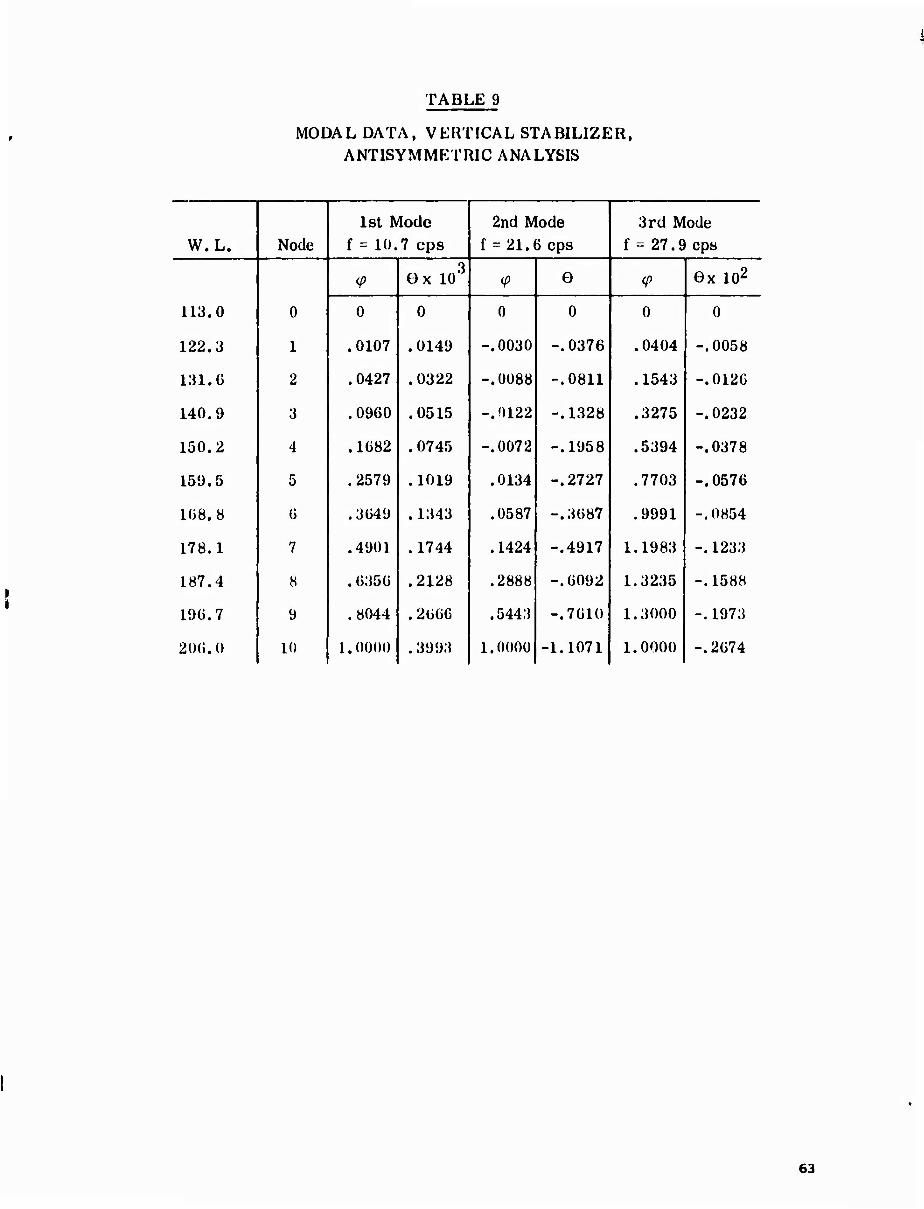
TABLE 9
MODAL DATA, VERTICAL STABILIZER, ANTISYMMETRIC ANALYSIS
1st Mode 2nd Mode 3rd Mode
W.L. Node f = 10.7 cps f = 21.6 cps f - 27.9 cps
0
<P Gx io3 <P 0 (p Gx ID2
113.0 0 0 0 0 0 0
122.3 1 .0107 . 0149 -.0030 -.0376 .0404 -.0058
131. G 2 .0427 .0322 -.0088 -.0811 .1543 -.0126
140.9 3 .0960 .0515 -.0122 -.1328 .3275 -.0232
150.2 4 .1682 . 0745 -.0072 -.1958 .5394 -.0378
159.5 5 .2579 . 1019 .0134 -.2727 .7703 -.0576
1G8. 8 Ü . 3G49 . 1343 .0587 -.3687 .9991 -.0854
178.1 7 .4901 .1744 .1424 -.4917 1.198; -.1233
187.4 H . 6356 .2128 .2888 -.6092 1.3235 -.1588
19G.7 9 .8044 .2666 .544} -.7610 1.3000 -.1973
20G.0 10 1.0000 . 3993 1.0000 -1.1071 1.0000 -.2674
63

w
(Q
o M iH t» $ o (N t^ CO t^ l> CD CO rH rH »H
o •n t* (N m O co o o o O o O O O 5 0» Q o iH iH m t> iH iH o o o o o o O O O
S • o o> CVJ o f-t iH o o o o o o o O O O ^ iH • • • • • • • • • • • • • • • • J3 m iH i 1 1 1 1 1 1 1
Tt< II
CO o a o m t* •^ o 00 oo m t~ CO 05 (N in in in co
"O o o co iH o «D Oi iH i> Oi OJ CO rH CO i> t* t^
1°. ® o t* "^ t- (N «5 a> iH »H rH iH rH o o o o o 0> t- in r^ iH o O o o o O o o o o
^s • 1-1
• t • • • • • 1
• • • • • • i
• f
CO II IM
co
■s & 1°.
o o ;D r- in in <ji ■* l> co CO O ^ (N o o o 00 o 00 <£> s co in co s •t t> o rH co m
G o c» oo o <N t> CO iH in ^ (N ai 05 o» o OS oo 00 t> m co i-t >* CO (N o (N m in in
?s • 1-(
• • • • • • • • • 1
• • 1
• • • •
CNJ II
S-t
co a» a o o 0> iH (N o> c- i> m c* ■^ M CO CO "^ Oi
"0 o o Tt« 05 a> as iH (N m N o> rH ^ ■^ N in oo
lm. O o o 05
CO a> 00 s in CO
CO iH CO CO in
00 $$ lo ^
• • 1* 1* i* r rH | rH rH rH
^ n
CO
o (N ■* in eg <£> iH (N rH m co (N O rH CO Gi o O Oi Oi (N •<* t> m iH (N oo rH m CO O l>
O (N S- o O CO m o CO CO CO M ^ t* oo Tt« in rH OJ
2» o • co •
co « ■ • o
t o • o • o • O • o • o • o
• o • (N CO • •
ja CM i-H i i 1 I 1 i 1 1 4-i ^« n
CO (U a o i-i t- <N t> oo 0> 00 t> <N s N t«- m co co t? o o 05 m O & ^ 00 CO o CO t» 00 o oj m
o Oi (£> iH M in '«f iH (N "t "* (N rH o O 00
^- o (N -* o O o o o O o o O O rH N CO
^s •
•H t
1 t
1 •
1 • • • w
1 •
1 • • 9 •
<n n U-l
T3 o 0 o (N "t iH a o CO (N r-t t> o (N CO in O rH
S ^ o & Oi oo o> CD (N Oi 3 ^ CO t* (N rH t> t- o m "^ Oi m r-* <N iH o rH iH 0) (N 00 |>
T3 CO 9- o (N o CO (N rH o i-H iH iH O rH (N in r- o • 1-t
• ■ • • 1
• 1
• t • • • • 1
• • i
• • i
<*4
o «o (N (N ■^ (N co ^ i-( m <Ji a> co 05 m in 5 o 00 O ^ "^ co Oi CO in TJ< ■^ in t> Oi (N in
• 9 o iH C5 <N (N (N rH rH o o rH (N co s CO t- o m O O O O o O o o o o o o c
■ft? "^ • • • • • • • • • • • • • • • • CO rH 1 1 1 1 | 1 f-t II
H-t
1 o iH (N co "* in CO t> 00 a o rH (N co ^t m z tH rH rH rH rH iH
co b- o CO t* o co t- o CO t> o CO t- o • CO
o co <£) o CO CO o co CO o co CO o CO CO o
• "^ 00 co t> rH CO o ■<* o» CO t> (N •
CO • •
o in b 00 <£> o CO t^ o ^ t- o "^ t» rH ^
00 rH iH iH iH (N <N (N co CO co •«*« ■^ m
c
i
i
64
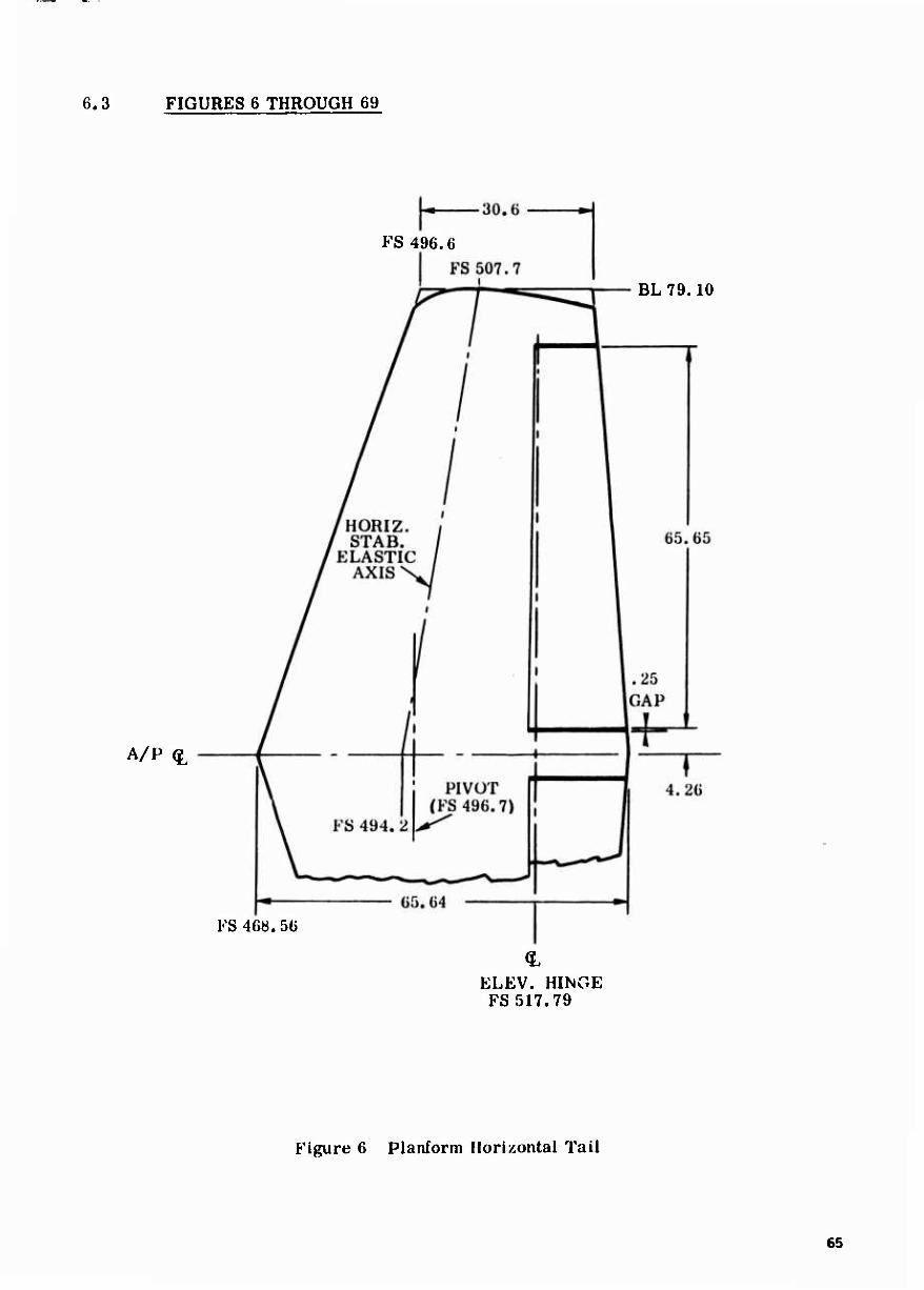
6.3 FIGURES 6 THROUGH 69
A/P (£
VS 468.56
FS 496.6
BL79.10
ELEV. HINGE FS 517.79
Figure 6 Planform Horizontal Tail
65
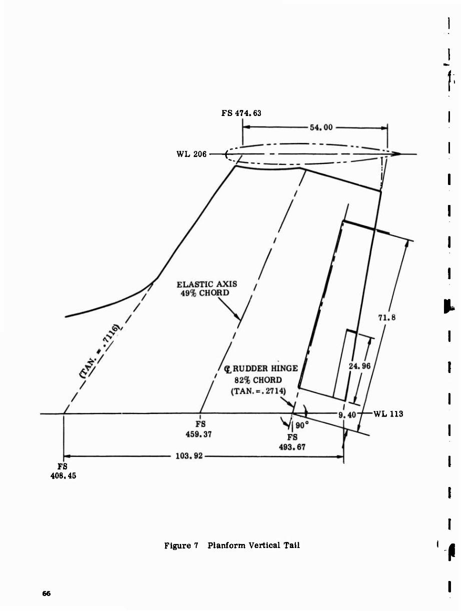
FS 474.63
WL 206 f
WL113
FS 408.45
Figure 7 Planform Vertical Tall
66
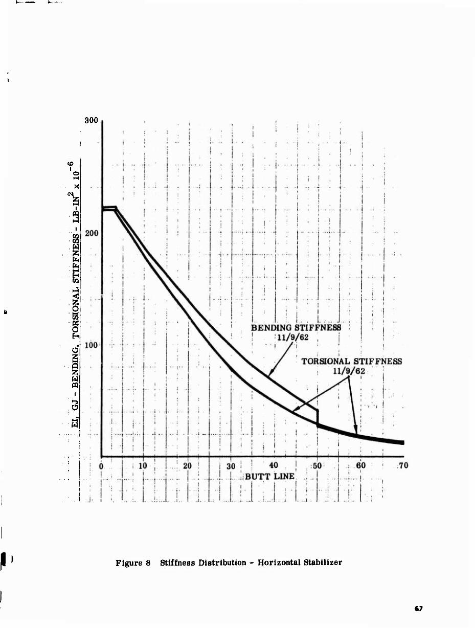
300
i
3
i a § H
Ü g
3
Figure 8 Stiffness Distribution - Horizontal Stabilizer
67
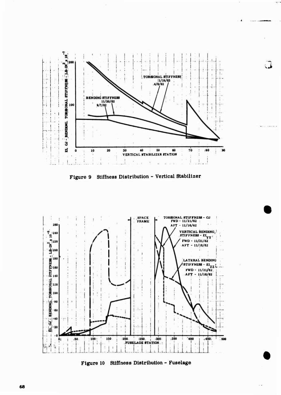
- ■ -I
! i
i !■ : i - t- ■ i
30 40 50 60 VERTICAL STABILIZER STATION
I
Figure 9 Stiffness Distribution - Vertical Stabilizer
a
TOHSIONAL STIFFNESS - OJ I FWO - U/21/62 : AFT - 11/16/62
VERTICAL BENDING,
Y STIFFNESS - El^
FWD- U/21/62 AFT - 11/16/62
LATERAL BENDINQ STIFFNESS - El ii
ZZ»t- FWD- 11/21/62: AFT • 11/16/62
Figure 10 Stiffness Distribution - Fuselage
68
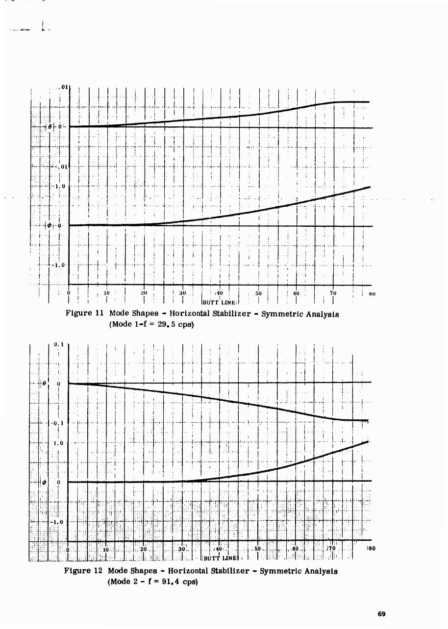
i : i.l
1 1 > '
1 i ^^
.-•-- '
.... ....
1
i
i • i
.. ,i ..
j rr i
- [.:■■
H
i
o L r»
.1 . 1
. i !...
: ■ •i i
i
1... 1
' i ■ i
' i r :
1
1 j
1 i
,:..|. .. i
-4— i
i i i ■ i- ■ ' ;■
L.„. -T* ''■-. 01 f-
I
. | ..
.. i
• -r 1 . '
- • j
i
i
i
...i... ' i
...I . . ... ...j... ! ... ..
1
| ; .... /
1 ;L
. 1 -1.0
.; i ■.
i
>|-0
■■[ 1
1 ■ ■—!""
1 . .1
... j ..
;
i .........
1 . ■
. ... .
.. -i„..
,.... i...
.. .t
i i ■.
.. ...... J.. ,:
' ~
i i
"^
1" ' i
■ i- -- l i i
i
i
1
i
...( ■
i
i i
i
i
i i
; 1 '1 -H T . 1 1
1.. 1...;... I •
' i 1
1
*
...... .. i
I
■ 1
1 ■
1 i 1 i i
1 ' I i
i' ' 4. ..
1 i '
--1.0- ..:
1 ■' ■
"I i
1 •
i " i i
i
i
■ -i--!
! i., 1
1 :
! I !
■ : ••••
i j...,
, i ! 1 1 1 1
'i i ! M , io : 1 tu , 1 1 ! 1 ! 30 . ; : ,40
* 1 t '■
1:1! ; 50 I j 60 ; 1 70 ; i «o
1 1 : i < 1 i i I 1 1 1 ; i BUTT LINKi ; l 1 1 ; l 1 i 1 i
Figure 11 Mode Shapes - Horizontal Stabilizer - Symmetric Analysis (Mode 1-f = 29,5 ops)
•"-
■
jo
i
.... '
... .
' . u
1 immmm
i ^—-
i f i ! . ' 1 ■ i
.w. ■ ..j. .. I
• !••• 1
i
! •• ■
i
i . .,
1
! :
■ 1
1
1 .:,.-. l
"■■■wft ^...^
-r.
-Ü. 1 "
11
1.0 j
■ - ....
■
■•■■]■ ■■
i .... .-:
::'
i
i —
"].: ...;i....
,... 1 1 1
.. . i 1 • I ........
! i
1 | .... 0**
.
i* 1
■ 1 i .. .. ...
i
... j. .. i
i
„.. „.. i
■--t*'*r
II
1 .....
r ^ -
1
" U-
■1 ■■ i
r^-
.... .. j.... i 1...
.. :. .i.... . i ...
i
... i. .. 1 1 ,;.. i.
. ■
. 1 ■ ; ,
'i'l
_.. 1 r : i!
i ■ i
i •; ; r ti ■
; i. ^
' ■;
-i_ —i r. i
: it i :: ■ !|
i :i
i
-rr . 1 ^l
; . rJ
' !
rr-
I j
: l
• :•■ • t;
■ .
1 1 '
: '■
•:H . ..
. :
1!
II
-1.
m i, ;
Hit
, i
0 1
ll ■ i
—tr rn i . . ,. i
1
IT +»
i •
H ; !, ; ;l
1 ' ■
It' I ; i .!
m ' i! i :: i i1
i i:
11 ■-+T -♦«,
L_ ! •■
-t-r i ;; . l
■ ; i
: .1
H: i
•"V ♦ft
—im
rr . .1
■ 'i
I.,
■4*
iiii,
. '. i
Tt?r
' i; .1:1
ill ■ r ;,:2 :,i;
o.: i.l
'■
i :.
-3 »r iBl
!J4
JTT
I" ) :,
LI HE
..:fi );! i 1!
i - ■ i
, it
a;! : : i , 1 i ;.
18
Figure 12 Mode Shapes - Horizontal Stabilizer - Symmetric Analysis (Mode 2 - f= 91.4 cps)
69
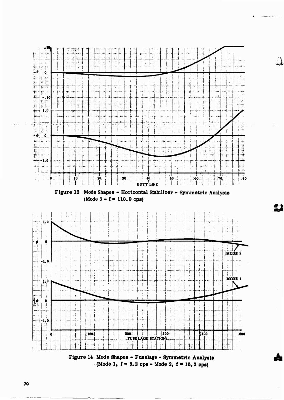
4
■^ t ■ ■
: ■ i ;' ! :;!' ,:,. !'..
... :;£ ■" ! ■ 1 ■ 1 ■ i:! 1 y i ; • i
;l:;i
r i'
.. i. ••i:
I -a —
i -r- i-i. — _., y.l —1 ■r—
1 1 ■
,__ i ; fSJ,..- LJ- ::A.:-
i H- I i
Lj..;. L.4-
* . -j.l..
,;■ "I i ' ' : ; 1 ' :
■ i J i i r ■ ! " '
•T- : •;■- ,... .
i i 1
. i
i 1 .
"" ■
■1 ..! :: i , .. i
...j... ■
■ .
-r • ■ 1
-.10 ■nr- :;: r ■
1.0 . ■ 1"
,. : . 1 .
r4~ :' i,
.,:..( . 0
1
i ■ ■
t '■.-•
.... ■;: |;
i
1
■ ■
.... ;
1 _ . :i...
. ^..;L..
■
■""i"
|..-
•
.... ': :
— —,■
... ;
I.
i
_...
L...
.1
. ..
i I .
';■
.. 1..
...i
! •
j ,
. -I ■
i, ! ■
: i..: i
—-t —
■■']"."
. -i....
' 1 " i
i
r.
■ • !
I
t... r : !
;.. i < .
: i.:rh n l > ̂ 1- ■ ■
'i • !• ■ r
;
■^ ; i i i :. 1 1 ! 1 j 1 ! : ' , 'j..
■:'
:rir
|! •:r*f"
";"r
' ..i.. i
. ■,,
4.. v
•■•;,: ■
I:1 ■
v •
*•- ••
•; 1 ■ I *
■ i
|
^u T.,..
.—|—ri ■ l 1
; j...'
.. ■ t
■ i; ■*tr
! ..
1
-..t 1 1
■ 1
1
I i 1
Li;, . ' 1:' 1 . • .„lo;... .
i -1 1 .:..! .,80. , 1 ..1 .40. : . '-^O..;.. .
■ ' i ' i ■ i ■ : ■ ' . .j.-eo.:.!. .. .Ii70f ,: • ..r.«
•■ ■ ■ ■ 1 1 . BUTT L» IE , 1 ■■]■■■ 1 .r;:l ■ i 1 1 i ■■■1 :■■ ■
Figure 13 Mode Shapes - Horizontal Stabilizer - Symmetric Analysis (Mode 3-f-110.9 cps)
1
1.0 s. ;
. .....
' • '. ._.
i .._ ,.,..
■■1
0 : iNv, ■ • | • ■ | •• [■■••■ 1 ' ' " '
, 1 1 . .... .. , ..!...., ..
■ I ! 1 ■
. r... .
i ... . . i
1 ; 1
; .. :.. .
i : ' !
: ! 1
■
' i
- I
...j.. 1
1
i
IMO DE a j
r" i -1.0
1 1 ' _ i.;...
. i ■
i
. i
-1"" 1
1
i
...,...
1 - -•-'-■•
.. i...
1 : 1 i
-r
r ... 1.0
...p.,, ■ i
"'" i
- —-r— i
; I. 1
1
•i r ;
-t- ■ i •
t
... - r- ■ t
- (•••■
. i
. -j.. . I
1 i
. i MC
i
DE 1
r1' i i i ' 1 ■ 1
■ i i ■
; : I
....... •-H -—
"^ '
t u
...j......
• i ; ..1 • A
i . i..
i i
I' i
...1. . ■ 1
1
1 ■i
■
i
- u.
1 j
t
„j..
....... ...... 1
■T
.....
i
1
1 ]
1
. .|. . —i-..
l ... .p..
' r ....
i -1.0 i ! "'"I ' ; i —j- • I
... ■
I ■ i •
i ■ I' t ■ i -
1
1 ... i L-
-! :;■
)i' i- t
. .1. . • ii iöo,| I :IMO;:. | i .! ,. isöO'i i _ 1400 .. i., ;M0
— • 1 •
1 1
'I M*. ._. _.4- •
j.. i
i —-t •- •"• "■"
i
..1, .
ruse LAGl :8TA 1
no« i
T
-- i
-••
L- 'JIL
— ,. .
.i _J
i
—j _j LL ' 1
Figure 14 Mode Shapes - Fuselage - Symmetrie Analysis (Mode 1, f - 8,2 ops - Mode 2, f • 16.2 ops)
70
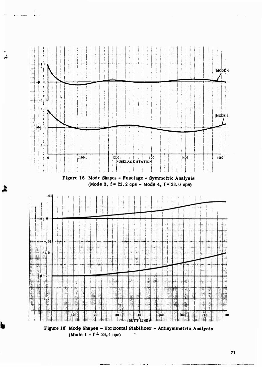
_.. ... • . . .. i, ..
1 ...4.. ..
.. ..
1 t
■ ■(•■ . ... ..
1 ' 1 —k... - . . - 1
1
1 i ...,
„. 11 OL i i ..,.,.... .. ....
1 ,..!.. . . t ...|
1
•■ -j — 1 ... t . ■ -r
1 ■ T ■ '
1
r-01-i \
1 i
■ t ■ i -■
.
" 1
1 ■ ■ "
_
MODE 4
DT TTTM
........ 1
' ! * !
i ■ . . . r
- 1 i
■ 1 : , : . .i .. .. j..
.
_ . t- .
1 1
— f—
r' .... •
-i oJ ■ -i i,
... 1... - • .... 1
■• .... 1 . '
1
--,.,. j
•1 0^ i ■ ! ■ --
1
■
i ■■ r ...
i l[:0|
-1 0
■ '
(
\ • I ■
;
,
c 1
: j , 1
_ ^^^^
.1 , ' 1 . . 1 ■ 1
.. .
■
. {MODE 3
1
1 ■■ .......
• '■ -1
;
■
1
1 i
1 1 1 '
'
1
' " . _
i 1 1
1 1 !
■ ,
■
....
> , 1
,.<
l 1 |2( ►01 1 : j
PUbELAÜE STA 1 1
I 300
TION 1
, •. 1 1400
' 1 1 1 ■■
. .
1 1500
i . i.-.. . .i... . .. ..
t
.- . .1
Figure 15 Mode Shapes - Fuselage - Symmetrie Analysis (Mode 3, f = 23.2 eps - Mode 4, f = 33.0 eps)
iiH jB0
Figure 16' Mode Shapes - Horizontal Stabilizer - Antisymmetric Analysis (Mode 1-f ^ 29.4cp8)
71
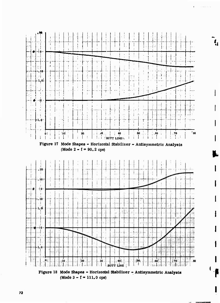
"."* ■
■
1
■ 1 . . 1
1 ....
I ■;
i i
1 " !
!
i
i
■1 •
1 i •
i
i ■ ...4....
1 t
i
i i
i i
i i.
1 . ,.i
i ■
i i i
i
i 1
... ] .:
1
i
t
i .i
i i
i : ...1
i
! i
1
1 •
.i .
i 1
T
i
■ : . —
1 i ■
-14- 1
....... F' ._■
:; i'
i
i
•01 t
- 1
i
' i ■ .....i.„.
1
......
i
t
i
i
....... . t i
■
1 ■
:. 1
. ;i :. i
; 1
-1*
1 1
... , , i
i 1 ■
■H i
.:
. ,:i,:. T
i
■ ■ r
!
i
.
\
' ' 1 ' 1 !
' i ' 1 ; " 1 ' i < >
, 1 ■ '
■;
..J_.. i
i i
i
i ■'•■ ■' •■ . 1 '
. ..;.... : i
...;1....
■i
• i ■
t ■ 1
.._j— :. i
..... !
...\ :
l-i.o- 1 1 '
! i
,. ,.|, ........
.; 1 i l ■
■ . i
r. ;
.i
!
.
1 (
1 II
i
i , 1 ' i ..oi ;
i ■ 1 20
i
i ' i ; 4o : ;».:-! ;.60 ; !
1 1 14. i '80
1 , i ' 1 '■ i • !BU rr LIN E\i i I i l 1 1 i i' t ' 1
Figure 17 Mode Shapes - Horizontal Stabilizer - Antisymmetric Analysis (Mode 2 - f = 90.2 cps)
Figure 18 Mode Shapes - Horizontal Stabilizer - Antisymmetric Analysis (Mode 3 -f * 111.0 cps)
72
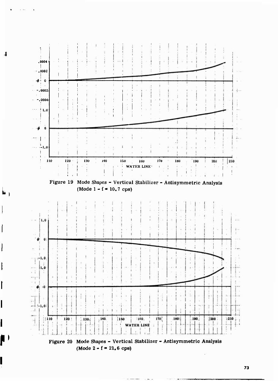
.0004
I '.0002
I I
$ ' 0 I
-.0002
-.0004i
I Uü
^ 0
■1.0
no
i i
I I
lao
i i
I'oO Uiü 170
> WATKU LINK' i
! i : I :
Figure 19 Mode Shapes - Vertical Stabilizer - Antisymmetric Analysis (Mode 1 - f» 10.7 cps)
Figure 20 Mode Shapes - Vertical Stabilizer - Antisymmetric (Mode 2- f» 21.6 cps)
73
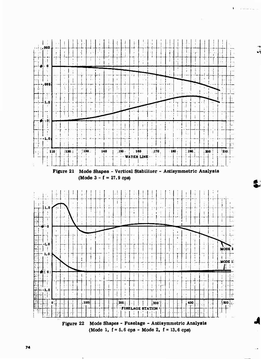
1
■
•;. 002. 1
-f- ■
.!
-0
1 j- ■
i
i
j
—
i
i
1 ■ 1 •
.4- _.;._
1 1
t
1
1 '
1
.. .1 . „u
i
._4...
1 1 1
1
■ 1
—i— . 1
1
1 . *
1
1
1
i ■ 1
1
1.1.. 1. .1,..
1 1
U- 1 1
r t ■
\ —-*—.
i
1 1 1 1
1
r • ■■■ i i
i
i 1
1 i 1 i
1
T 1 ! ..; . 1
■ \- ■:
t
I 'T i —t ■
1 1
._j,.,. - !
1 ■
i
1
1 r ■ I. .
1
1
1
X. 1
- T-
i r .002 ...j... 1
i
-4.. ....,._ 1
' ' '
1
1 ■—!
: _.(. ■
H^ ; 1
i
i i _
[ 1
1.0
-,01 1 1
1
1 y-
i -i-
• 'T - .1 .
) t
—i—
!
.._L.. •-t- 1
i
... 1 - ■
I
—r._ 1 1
1
0**.
| ■
— r ■
1
— I- •' • 1
1
..,.. ,! . t .
:
>-
1 ,_!_
^'' ■
...... , 1 i
1
j
■j ■ 1
I
1 —,.. .
1
,.*-. —
i 1 i
1 !
1 ■ ...:,.. 1...
: M - •■ -i
| 1 ■ 1
.: . j , ... j
._i„... i
1
j
1 ,—
!
1
l.Ol
:
■
1 ■
■
;
—t--
; 1
<
; 1
1
1
....... ■
0 '"
i..
10
i
:|1S i
1
to.(. ,
!130! ' 1 ....
■ 1 ■ .._L..l... ;...
140 1
„.._L:...
IJIM. ] ! 160 j '{170, 1 i 160,
-• '-WATER UNE - - « - j - j ■'--
• 1 1 i ; • 1 !
i.iw,; .
1 1 *
■[■ ■ 1 1 ■
j 200 !
' 1 ' 121 1
.1
Figure 21 Mode Shapes - Vertical Stabilizer - Antisymmetric Analysis (Mode 3 - f = 27.9 ops)
1
1 t ... ...
!• 1 1 • ■
1
_. —;.— ~
-- i — ! 1
1
i ... - .
1
- .... 1
. r :n'sr\ i 1 . 1 1
T
.. i.. ; * i
•••'
r .... .' 1.
...... ■ '
> I
. ..1
1 \
1
; 1
•4- i i
. _.; i
1
■ 1 1 i
1
1 1
1 1
1
•-t~ 1 I
1 1
■•-!•• -
t 1
)
...L -f-: 1..:.
t: 1
pi-
U,|4
rr-
.1
>--0
i
'"! i
-1.0 .■ 1
1 1 —I" ■
i
—N
i 1 1 . ...
s 1
■1
~~
■ 1 ■ 1
1 1
—j—•
t
i
i
1
1
1 ...1...
i
1
r
1 1 T -
1 . i
. i 1 1 >
IMC
. .1....
!
DE 2
.;:■
~'~" 1.0; s, ...... ..J... 1 ~"t~"
1
—1_.
1 1
._ 1 . ... i._ 1 1 ■ ■i
... ,. - 1 1 T T" 1
1
■ -v ■ 1
. .4.. •
1 ■;1"
(fi •
r 11
4 ■io
1 ...1. „ 1
^ ^
t i 1 ■
..j—
■
1
i
1
1
; ■
1
......... •
. , ~ -HOI DE 11
■—
j ■ 1 ,
' 1 i : 1 1
1 1
j 1 1
1 i i 1
1 I i i
1
li
■!
trr- rr
■ i ■, ;.
-1.0
1
1
•■,. . _
1
...1. ■ i
1 j "1 '
...j 1
i
1
• ■ f- ■ 1
-4- i
1
..._♦ ...
I
1
1 1
1
.4... 1
1 I ..... ... ~x.
,,,,
1 ' m *: ' ?.T '1 '
■ 1 1
- l 1 1 1 1 1
1 1 1
■ 1
i 1
i ■ti-
'"' ,■ ( JOO| 1
i2?0-!- 1
i (300 ,* >0 '''.]"'.
"1* »0 '■}.■
, ... ■ ;;: ■ 1 .1
;! 1 i; i 1 _ . .1
i I l
■ 1
r uDb uAUb 01 A 1 tun r
if M i rittl- 1
... L* .
r: .i 1 1
Figure 22 Mode Shapes - Fuselage - Antisymmetric Analysis (Mode 1, f = 5.6 cps - Mode 2( f = 13.6 cps)
74
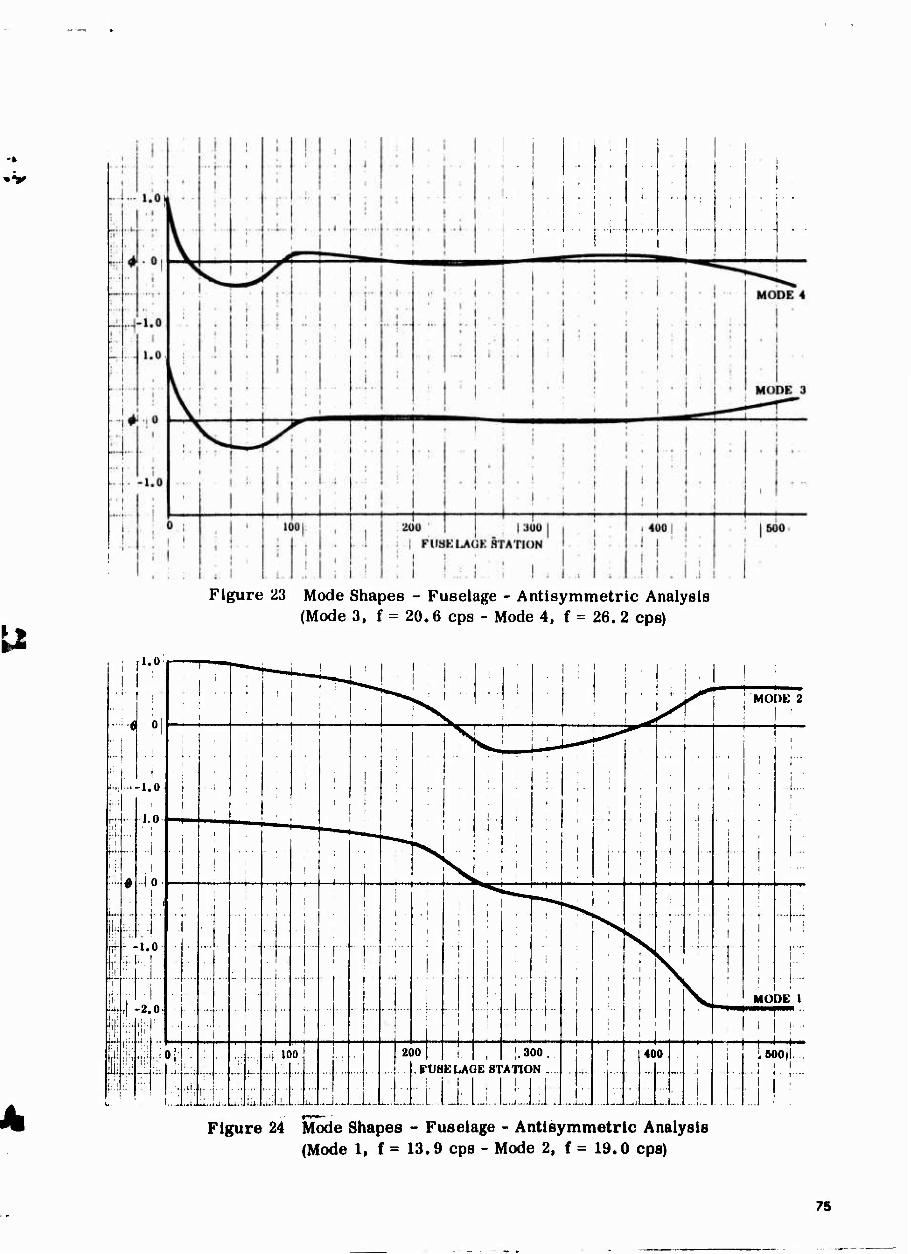
Figure 23 Mode Shapes - Fuselage - Antisymmetric Analysis (Mode 3, f = 20.6 ops - Mode 4, f = 26. 2 cps)
1 1 1
!
0
r- i
i m—i-"-^-j^j ^ i
1
1 : !
1 ' ■ 1 ' i 1 i , ! '
■ 1 i , ! ■ Irv' ! ; ! 'j^f ! MODE 2
L... j
-1.0
i
I i
i i
■
] t
^
1
■
i
•
. .
i
; I
|
i
..i.... i
fr"
■ !
U...
1.0
i ■-1
1 ■ i : i :
-■
i" i 1
i -1
.i .
1 i i
■ 1
l
i.
1
"*~" ■"■'"-
i
♦ ..i 0 i I
1 ^V. ' ' i 1 1
i
; 1 1
1 i i 1
^1 1 , : i i 1 i
,..j.., i
jl, ■ -
1 ■• T ■
1 . 1
1 . l
t ■
; r " ' i (■
i ] ;
■ 'i
ii; ...
i.o — ■
.. j.. ... i..
1
1 .......
... "i"
f
i j.
i
- i ■ t
i
1 N i
w
t
i i i
fe
:;•
i j i 1 i 1 ■ i 1
i i
i i \ MODE 1
-<5. 1,
lii'
1 • ■ t
.. j.. i
1 l 1
1
■■■■( ■
1 1
■ |
i
1
i !
; , i !
, H »! ^
.<; loo 1 l 1 200 | 1 1. 1
|.300. i i ■ i 400
; 1 \ »00)1 ..
■■ 1 •'
,1
i... , .... i FUSE LAC ill
IE 81 ATION . 1 1 1
_ i i i 1 . . i i . ,....
1 1 '
t*u a. . ̂ u- :■ .*.- J_ i ii*.. J ̂ i.- -.J J..;
1
—u .„ ... ... ...:,.. j '
Figure 24 Mode Shapes - Fuselage - Antisymmetric Analysis (Mode 1, f = 13.9 cps - Mode 2, f = 19.0 cps)
75
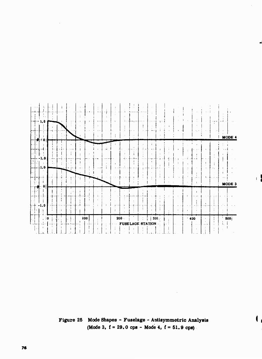
.... .... ..!... .. ! i
■ •■■
''■ '
|
■ ■ ■ ,
— '
1.0
^N ; ■ ■ •
... --.,...
1
■i •
r 1 !
1 !:■■ ! 1
■ 1
■40|
i
-1.0
1 ^
■ ■ ■ (■
\ :
.......... , .;. I . . ,,.... | , i ' i ' < ' • ' ' 1 1 MODE 4
.... i • r ■
I ■■•t ■
I
i
—1 ■
i
■
-■ -t-
.... ;
. .1 . .
1
... !._ i
]
r—— I
i . ; | .
: 1 .i . ...
i
|
:
(■■ i
-
■
1.0 I ^^^^
i :
1 "' - 1- 1 i !
i
'
A
■i ol
■ -f I ' i
i "^N
. ; I
■
1 . 1 , | , . I. . . ... |
MODE 3
-1-.
■ L i
1
i 1.0
■1
.j... 1
. j.. 1
I
(
i
i . ..i....
i
.
:1 h i J
. ..j ... i
■
. . ,
1
■
■ ■
i
t
■ ■
. . . ..
] .. . . . i
■ *
t ■ ■ t • ■
1 i ■ i ._.t_..
.. i , iO ;. . • ■ ••!■
100 200 | ■ 1300
l 400 1 1
1 500i
i ■ ■
i
i
i
i
.1... i ■
i
i i
.... FUSELAQI
i ■ 1 ■ i ,
] STATION
;l,„l • :
' 1
1
' ! I- 1 i
Figure 25 Mode Shapes - Fuselage - Antisymmetric Analysis (Mode 3. f = 29.0 ops - Mode 4, f = 51.9 ops)
76
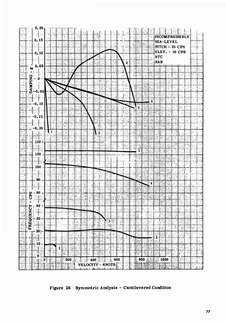
Figure 26 Symmetric Analysis - Cantllevered Condition
77
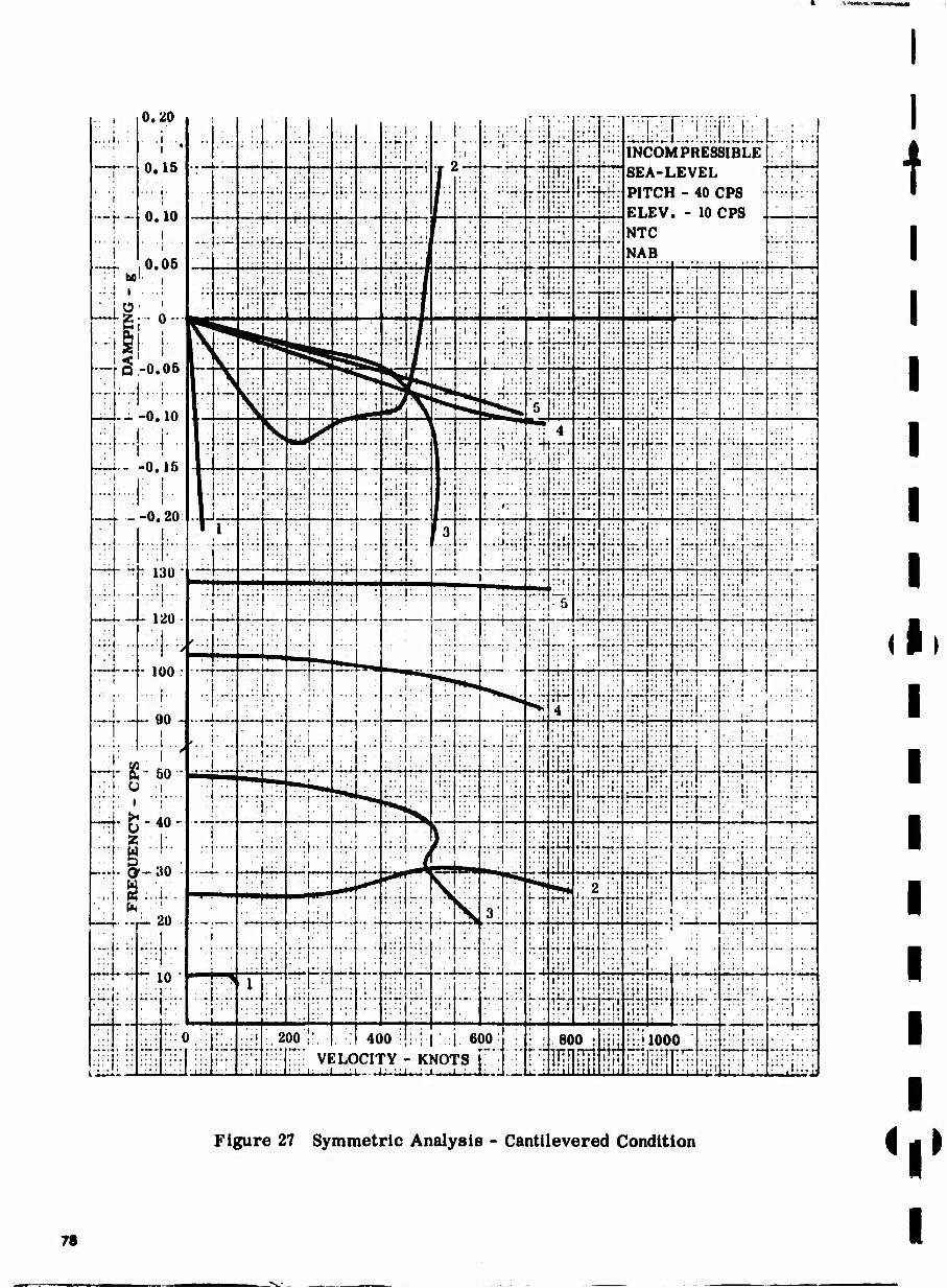
—f- ...,.
o.zo
i- 0.15
• • ■ i-
0.10 1 i
0.05
.... .... ;'•• ; •.;.■ •
r T. " •
: "i . i.
; i':
■ M ■ INCÖÄ ■
:ii; ^ij;;'
3IBLE : : j. | fPRESI
„..; r'1' •'■:• --'• .».. -••• : :l
il.i
:
L:!.i ; i
i i » i ^ - '
' ii rtr ! I!
ii:; Jlil
SEA-LEVEL PITCH - 40 CPS
ELEV. - 10 CPS .
NTC NAB 1 ■!■■
....... ..
—: •:- r-;; ::r :;:: :i..
•-:
i.:: m • --«
1 ■
i ■ 1 ■ .11 II ■ n
..i. i i' ■ i:
-; toi. ;. • t 1
—f 0,-0.05 ■ 1, ._ . ;
-^J.--0.10
_n iK
"v
•:T ;i;!
rr- rrr '•"': rir .:.: i — - • • i
;':! I'I.
. .1 .
^['^ ::;:i;:; rrir;- .;; !■;■:
:: ■ j •..
■ ■ ■*■■■■
V ^ i ̂* 5?
i
I r" i'i r-r!:i:: • • t * f - •
;:lj
i;;; rjr
l'|,
Tfri
■ ,.!...:
f— ii. rrr ' ' i . ■ ' I ■ ■
1' ■ N s| -r • »♦•
i ■ ■ t pfe :■
I'-;
:"T;:;
's"
i ,:
:r.; ; ■ . t
'. i :i :H: rH: riiir
:::. I.;;:
":• —
■.■(■■
■ ; ■ ; t _ ■ ■
( H=2 :!:! I!! 1
••r i ^
•i - ^-r
4 fyrrr M':
:!:: iii: :;I; :;i;
■fr-
■"}''•
.:;; ;..
■: 'i .-
'■'
1
:■ 1 * - i
-0.20
■;,:'
: M : : ■; 1: ■:. .■'i
—-
. .. T ■ - ■
......
■ ■:: ■ , 1-4
t '• * • ::i:
'Ill
.' t. i
rl\ :;:;i:;;i :;i .
.... ■ ..
-*■•♦
•:•• -■•
i~_
r -r ... "T** ;;:! — i.... ' l. .
■ i ■ ■ .:..) : :
•::: .
■ 130 ;
■ .;r ■ ........
- 120 -
.... . .^
■ 100 r ( ... (..
- 90 - i
1'
I rr- i *? ....
i ■ j I • ■ i
:::i ' It' nn
■••!
■rn I !!. ■ i - • iii;
rn: frrf irr: .iii i :: :.
ii;.j.:..
:, l: ' •
' I
r\ .:::|. ..
■ t
.■i
■ ■ i
■■;i; „
;• ' i , i'. Iii;,
• . i
. . • ... i
i'-.|- ::
1' l ■ i
.... . . .':. :::" ..;... . ■ ■ ■ ' , .. :|;
■ (.. . :: ■■..;-■.- .....
■
■
— 1
' .1 r ..-.I- J
f..', :u. ::!.;.■
—-
■
, 1 ._ i'i
r-r: . • *«. rff: ~u ^f«» ' ::!:"i .........
—
.....
■.. 1-, ■ 1.. ,.:::•
. . . , .
! . i.
■ .!
..:_
r '•!
if11
4
.1:: :f::
;•
,: ;
i: :t ::. :!;;j: .
■ I ■ :' 1:'
i .i .:
: .
■::•
•••:
.. ,
::.. -;: ;'.l ;... r;: ■ ■ 11
'-r;t
!' ' »*-♦*
... I
■;:;; "':■■ r-i
/.'iii.i 'I p, ou
,;,{. u i
-4- g - 40 - ■ ■ z ■ ...
— mm\mr 1 ■
., . ,.,, "TTT ■iii
1 iii
'Ii:
I.I.
....
i..
;;i-i;:::
:' i';'. *"' ■ ^^^^i
s ..;:; :r:: r.r: ...» TTT ; i iw: ;
. • • i i
' ■ i' ' '■ 'I'-
..... |....
i i
::!■•■•
i
i" ■ .
J h mm
3_
1 rri 141 : jj
i • •!
•v.: r~ :':'
■:ri,,; ~:l--- -ij:::
i ■
::: ■ ■' ■,;
" ;
■
• • • • ■
• • i ■
% f-f
;l;;
;;'2"i:; ht; ';•■
:::'v:' 'i1:
l
TT «it ,
:■■]■:■..
* * --r r~*-** rr-p-1-r
i!i ' " i
i....
■ ::i' l
■•:L :
.
i.:ii ■' ■
-- ^,4,
■ t < ■
riff
i;' i
►-;; ■:-;
..:.;|.... 1 :
':;' • ■•■
1 . :.■
u ■:
:i::'
I ':'.',
■;;;;;■
.:;: yrj! ilii
r;:.:
HrrHv :; ij .:
';i' :i:. ■■:
:;:: • •♦■ '-H-
:::0 ^ji1 ■
ll.i.
.200!;,
■;'' ;■;: VI i: ; • * ■ I ; . : •
4t >0 :
?Y ■ ■ Kl HOI
6(
rs i ;,.
)0 600 : P hit 1U1
i lit 1000 rrniiiiiT:^ iiii ;:l -i: iii;
I
Figure 27 Symmetric Analysis - Cantilevered Condition i
78
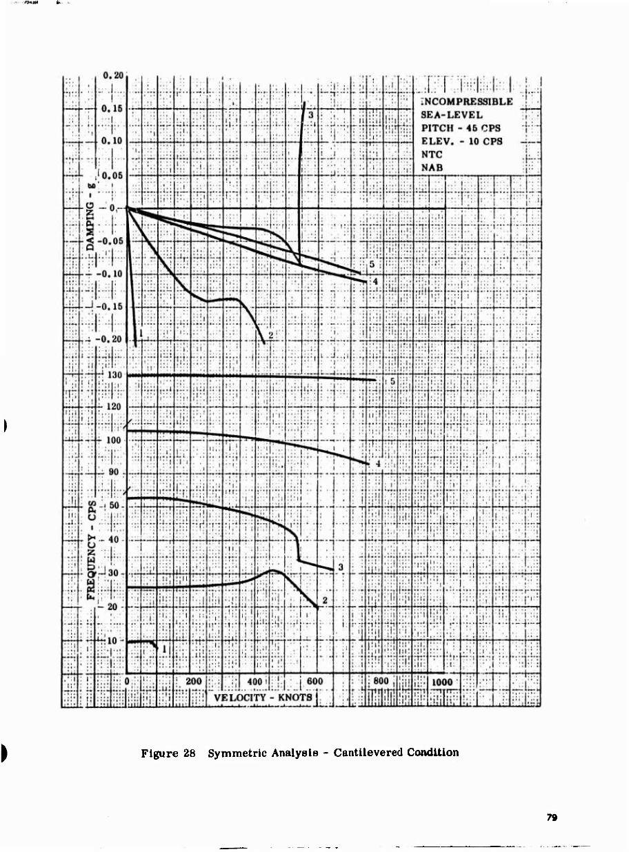
Figure 28 Symmetric Analysis - Cantllevered Condition
79
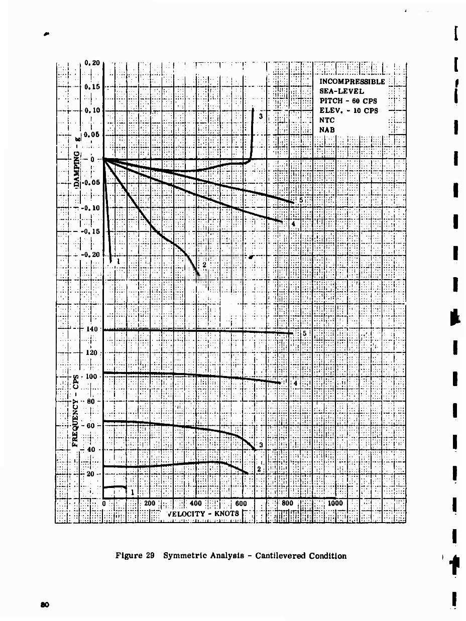
1' >
hi-: I i
l--f— .. i..
i
0.20|
■■!■
0.15
0.10 1
: T 1
•:-
;■■; ..;;
.;' • .. ......
' ■ i ,
' 1 • ■
■
•A'.
;i.;.i
. ;;i: ;;
: üU
. iT|: •■ rTtji-"
1 IJ-M i •rt:*:::
INCOMPRESSIBLE LJJJI SEA-LEVEL hi 1 PITCH - 60 CPS "j H PI Cir in nno 1 U
m. m* '. '. u». ■•;:- "H;; :'"' '- • .;:.;
r. ■
;■,
-: irr '-':'•
'.'■'■
i ■. "
f.Tr
;';i .i '.
- :
rrr
i.: i •::;
Ü 3
11 • ■
: :|;'i:
i :^i iui
NTC NAB
1 „i 1: :
T ho! •,
Nil ^
'.zr, • t-r*
< ■ i HTT »«-*-•* (••W ';...:
; f; j';
< • < 1 - ■ •
-S- L
iiii i " ■ ii; iiii; iiiiliiii -r.-M':'-'- i:::!',:i
■irf • 1 • :
'. ;
■ i ■
S •: ■'
5» T'T
i .■■•:
: ,i!i;;i •A'-". iiii
nil ■iii nil ;■!;
• ■ * • . • 1 .
... i
■ • i ■ i-ir- :. 1, :
'.: i: ;
,..::
—, i •: !!ii
H" -0.05
i i
[-'■■I- -
1 "V
^
£zir
1 ■ ;> s HT
I:II l!i! :!i'i
• | i
rrrr * >*' ;: i. i: i: i
.ii: .. ■ -:-:ir--l
.. ... .i '...'.
• * ■ ■
■ 1 ■ •
• ■ S:.r!:; .'.::. ..■i :: -u. IU
■*•:•
rrn 1 It if'-' :-,i: ,.;.; • ■ • t
i.ii ;;;
k. . H
V ', m • •. iiii 4 ...,
iiii tirt
t t |
iiii mi iri-i •~i
: ':
•.ill
... i;ii.L„J :ii:! :
1 '''
1 '
1 '.: -1
r v. tu
■ ■ 1 ■ 1 •::- ::; !^S s 1
■ ■ t
^
::,i!!' ; ! 1; ■;!:
•iii
• ■t*
iii!
... .■lii iiii irr ~M\
• ■ ■ • i «I ■ ■ t ■ i
:_:i.„ J :: 1 : ;...f '
• i:ii: ' r.iii.; ;i ll': TT"
X «f ■ ii
irr ri*rr,"' i • ■ ■
U —
.:.. \ i;:i
,. '; :i
i 2
"i
■rn
:.■;
.
i ■;
; ^
: i
ri
i I i i •
iiii IT: ilji
i:,
i >:." » • ■
ifh ;*ir »-••^ I. ^«
•'iilif
...... .. §
:::: 1: : :iirfr:: :;::i ;:
- 1 ±n •
.
-—* :i'.
^- 1;:,
■"TT In;
iii1
::i!
■ ■ 11
iiiiii^i : iiliiii rri:
.;! :;::|; :, ::;:|;.:: P::|vi :::. i.':'
Miil: A if-h-i ■ 1.. ;
.;.:
•j:
' i
• it
-«-»-«• ;i:,
t'ff : I:|;M1
If' i;;:
.lii. ■ ■
—^
■ •»• i : •
_J-J
h:j; - 120 r
. 1 1 t\£\ \
^-1 '; : ■;■:
:'n I j.'.. M!"
■
i
•
1".; i 5 i t • ■
'iii iiii
iiii ; :; *
'i": ' :!i i
1 i
t
:". 14 < t ■ ■ ♦
:.!: .,»i- r-ii trtr
i * •
* • i ■
ii'-
'iii
;:i:
■ • •
i-r t <
• ■
; : I i. i .;' i 1
::" !- mm
•1
... . ^T *-*.—
iy ; :j
U.l.Ü.;.. 1 '
JU -
■;:
::-;- •ir •»• • ■i-; : Ü ;;i: rTT > •. »!' -rrr LI
T-rr i Ü
rirr illi
Trrr
Ijil : 11
■»'9 1'
:,:: iL:' t . i •iii
1 ■ I 1,1 i
I ::
..i>
":':'
... R . : ■ -':
iii: t • ■ ■
n, ,:
; ■!
i.ii
ii-i
. > *
',.'■] "., .1 •:::f- i *; .
[*••- *- •-•-
iiii
;.::
ill: • iii ;T'' ' 1 • i : ii 4:r: :: '
:"i;t:"i|
•
■ . i
r i
^ _ Art J •—
— • «* ::i
i '..
::.:;
■
; ii i ji i:i: ^S ,3 i ii H; -**-♦■*- i iiii
jjii * 11 • ■ I '
iii:.
WryA
- t;i
-20-
; ,'
Mr ' ■ i •
1 | TS :;;;
N Ik';
; i.
2;
t ' ' ii:! riii hi
i i;
i .
' i * i iiii i'.
ri-i
... i .. i
i > • 1 TT!" ;.,: ••
I '•:'■:
.i: : i; t ■;
;;•: i
.I.- i :i
■ . i .
;i J * * •
:■ i
:.'r irrr 'A:'.
'■v.' .1,: iii: :!i: ..',; ;i:. '■.'::■
■■.;!i"11 „_ij:i.il T:iTi;"";1
... i. . .i I ■»
; ;;|; '■'
: ■; iiii ::;]',■ iiii füiir
[rr'l * '
'—" :;. ( ) I:
i t:
: 2C ,0i|::i| . I 1
ELC
4(
)cr lo ■!■;!; rv- k
: i600
NOTS \T', ..:.
' I ! 800 j
IJiii'iili ='!i
iiii woo rnttr-Tirrr; : :: . :; I::I i.:;l;.iil.ri iiii
r^- ;.'.
1 ' 1...! J
nil
Figure 29 Symmetric Analysis - Cantilevered Condition
80
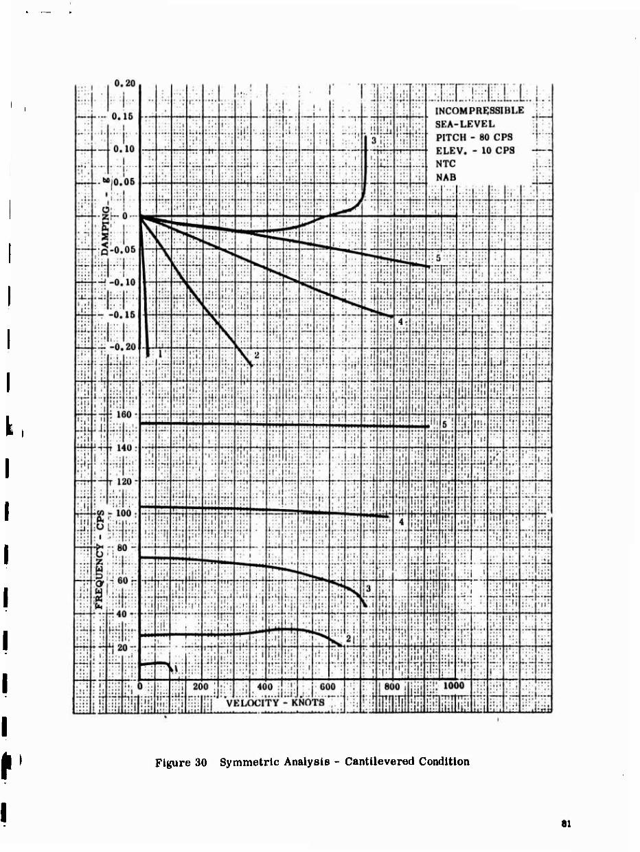
Figure 30 Symmetric Analysis - Cantllevered Condition
81
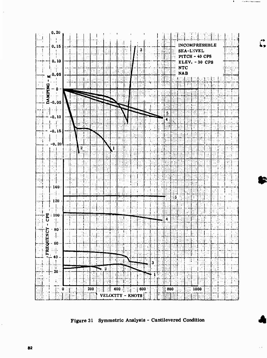
1 0.20 . ■ ■ [• ■ 1 y : i ■ ... ::
i , j
:...! i ,.i -r. i ; i ■ , J i: . .^ :.'. l^|_:i.:.: l_:.;:i;;i^L:: -;.: 1... j
•—j-.. 0.15 1
...... i
0.10
■
1 . :
w - — INCOMPRESSIBLE .
SEA-LISVEL —r-f—-j
••: ..;. :... :\: -• ■ •
... . Mii.i
■ l:i:'
i » •
; ! PITCH -40 CPS ■ ■ 1
■ * 1 ; i.l,.:: v ELEV. -30 CPS j :
'i -- .;.. _;. .::_ .-^ :.u ,..;. -- ..-^ .;:; 1 ■-•• -"-'••- -.J -i»~ — NTC ■'■•':;■.■
—r hB'0.06 ;.: :;.: ;;' I.: ::J: :':; • ■ t
• NAB ■ . ' 1 1
• «««• :;:H r- ■r-rr >*•• ,.-., m ■
\-H-'rr :;-;f :i;.
■:trr :■■. ....
;;:i ::. :.,!.'■•
l:: 1 : '
:!■!■■
■—:-:-H
m. 1..»•
^i _ *■ •
g •^ i' ! '
,.... m rr— r.^- i
• ■ i.i!, * r" ■ :: i;:; — U-l. ,;~ :'.',: :::!::::
:■ ■!:: . . 1 i . ) . . . >.^l.«.„^l
1 i S _ft AR 1 1 ^» «w* ̂ tif^ L ' 1 '. ' '■, L:' :_■. .. * ::i. :;:: :;;: : ■ r: :
L. 1 i ' 1 r\'\ St « /\ 1
V ;; '{■'■' ■rrr rrf' -rr ;•?" i 5: 52
,: .. -•:■ rri
5 ... tiir ■f::- :■'■'.
■ : ■
: 1 .■ :- :i-H
p—1 U, 1W i i r ' iV' ' • . ::: N ; ^ 4J :■:'
. * ■. ! 11 i •I'M': ■
'::: I... ■
i •
r~t- -0.16 I'll
1 i -ft 9ft
'\\\ m* S ̂ > ■' I
• «-** " 1 1
-i. i±r i ; '; t
I "
■•>»«>»
i;: f r. ♦
:; ■
•»'■■•
■"T" ■ *'. ■ 1
1 ■
:.M :: ■: I.-;.
1 : r :
N ^ :
«-•-. —( --•• ■.111
■ . ■
i i. ■
T T1
F :-::: *-•-.. ... i ri- •r*«
■ i 1 j 1:1 „..,...
': 1
• ", m ..... A KL i-1*
■^
4 . .
: r;'
TT ::: ;r:4 *rr .... irf
. . r i i
■■.\. l! ;:•
ill. ■■'• ■ 'i..;
■ 1 i ■
r- "^ i:i t'i ;: i ::::i:::; .':'.
■" ' ■ ■
it i-iU !-i! •- :i*lL ■i~.
L~-j—, '..I
---|—
■• 140:
■ i i .... i..
■ 120 i 1
... 1... , l
• :-
;:.. . ■
.:: .. ; 1
1 i : •'i :;: :: i ''»'.• ■ . * : j .' ■ ■ i 1
■
::;' • ;i.
•r ■•' !:'■
in' :r\y.
;■ ■'
';;'
i;:
rir 'rrl- -:••• 'Ill '.:'
: I
....... i
11 i
...i.J _.
.. .j...
■L ■ i
.: :i. ;; i •■•■:I:._J •- ■•■ ... ■ l'-l ;ii. 'iL
: i:
rrf;
'!• 1 :■•
:'.
:
1 i i • t ■
L ' 1 , , i ; ■ :■■ ; A ■ r
■•i:..
■ i
^11 '•.".{.':■ *:! •:
' mÜTmm
1 -::.|...
. . . , ,. ~i jrf* T" *-«-♦■
:,;■
;.:
i i . ::-
T— i,.
■ .'1
1 i
■ 1
h-H-Jg i 100- \::.[.o ;}..
: : i ;
III ' hrrf-&- 60-
;.:!:;;. ^r
.:. TT"
• ■ •
4 li;
•::
frr- TT^
-rt . !.,. ••:;[:•:•
■ 1... : ,; .■
■,:,l: ;
i ■.
■|.:
r " ■
■ • (
; i.;
•f-M ■•
1 , . 1
••: ,:.. ;:-- ;•-
ai-
::: rr. :!;
-- :- ;.. .■ :_ : 4..;J
: :!•■
. ■'::
■.;!■ ;
... .. | ' ■ i ■ ■ ■
r*- -r r.'*
■ ■ •
• >■*•* 11.. frr ':'■■ ■i ■ ,-: -• -- i 1
| • i
■ ■ ' '
■ ' t ■ i
I 1 ' ' ' 1
- 20 •
1
rf
::> 3
■ •
'ir ;"!. ...',:: .:;i;:
. ■ i ■' i : p" TL ^ ̂ t. 2 •
f>s ft** ;■
. . ■
■ '■ i : i . ' 1 !' i:; .... ....
;', i.
:•*: 1
1 1 ■ ■
... '.;
*"■
.'; 1. ■ i
.,... T " ".''" ■ :r I'"' .... .: ■ ■ j ..
*;. i -1 J-o f J 200 '.'.. ;.; 400 ! ::! 1 600 !' ' '800 • ■::; 1000 r:r ■ ....
■;:.
1 •h; i I. ; 1 % m VELC rv - K NO TS i... .-L
rrrttrr 1 ! ;:; ::: iiiliiirv
i'.
I L- • ■ i ■ •' i
■ r '-J
Figure 31 Symmetric Analysis - Cantilevered Condition
82
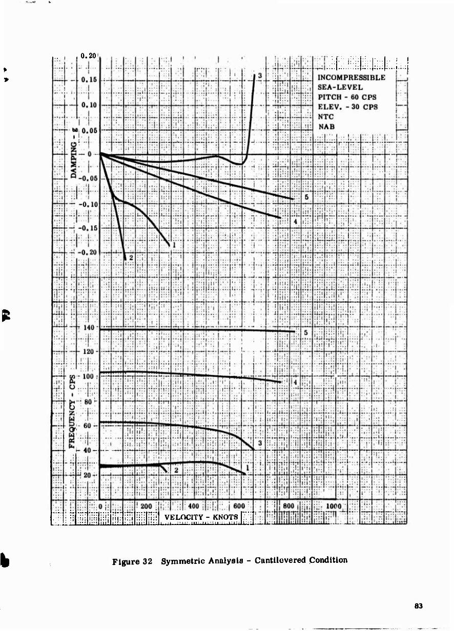
0.20
mi ill uu iiH VELOCITY - KNOTS P' ' Uuii '■ ■■"■ MKri::.! ■: 1:1:111;-
;;!:(:;:J:;::|^^:
Figure 32 Symmetric Analysis - Cantllovered Condition
83
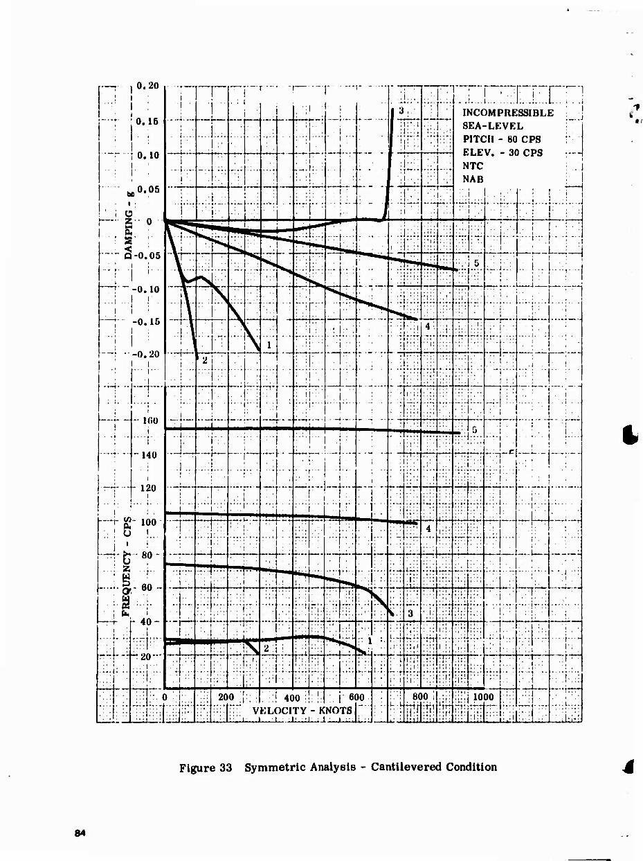
..... j I 1 1
i ! '
i ■ • . . 1 : :! ■
1 . ; i
r .... -
i 1 :
»-—•
1- 1 r— i 1:. :
I t
i . ! ... ( 1
'"
1 ^
1
E ;. • ■
i: ;■
;••:- ,..: i ..!. ..1 ;.1:...;....L.. i . .i INCOMPRESSIBLE • j
1 i U, ID 1
. .,.■.
—> -r—
::;.;1-,:: SEA-LEVEL i
PITCH - 80 cps ; ELEV. - 30 CPS ;—1 NTC I ,..i NAB i 1
I U. IU
1 ■ : r ,
[ «,0.05 ..^
1
j :. '-..
r: ! !', :
' -■ :
'•:;:
;.:.. I .-i ■■
i.._,.._
* ;:'r
■ 1 ■ ■ 1 :
i' LJ :
• :
■.'.\. ■'.
■;rT:!-f;: - ■■f:--- \ i ! M
• . i ,: :. :j ' fi u ^^
^iill' ,: • sE .:..,....
.. .i ..
:j:-,i ;:, T :..
■•4: t-r1 ...A:'. . .1 1 ■ H . ft \f ?
• i . :
TTT"
~ r S-0.05 1 •' ; i i
[-—T --0.10 ..-! • ! 1 1 . II'
L_j.„ .0#lß
1 ' 1 '■
i ; i
:: i ■ | .! i .1
: 1 ; I
) ^J" ,"• ' ! ....
'
s !■;•:
■
1 ..
:Ti; i iv! 5
V :ls |
' ^
11
I
1 ■ :::: ■i;:
t
;.;.| • : [' ; ■
^_ _j
• it- JA
i T
! A < i
i .. i "
—i—
i
rnrr" , ;:tr
1
■: !:• ;
i ■■
t
. 1.. ■■■]■■■-
. ..i;... 'H" •
i. j
......... 1:;
1 . 1
^ 2 i : ■|:;,
I
if. . .
: i 4;
"i;
:;l; ;H:- 1^: ;:-• '...': ....i. . 1
1
1
1 ;
I j I
I " 1
i t
-U, ZV I
:—r—■
• - 1«0
"140
i
- 120 i
... *. ..
1
■TT*
: ■ T
i.u ;iji ;';;
;;" "- : :
: i; ; 1 ;• : i ; ... , ..
■
—L- :.':
h i: It!
:.i.'. i i.:.:|
■ ■' I ! '. '
• • 1 • 1 ■ 1
..l .;. .....
... mm
i
'.".'. •'••
.. 1 ■ • r '
1 ■ .1 ■ 1
1
i
. ..j .;
. 1 . . .
i
i .
. i ■'
;:.■
:!.. 'v: .■::
■
;.■;
.
: i ■.
■
- ■
■ . 1 > <
irf:1 ::::
•■
1."
■ 1
h-r g- 100 ■.: 1 O !.
U-g-80-
[....;.§-60-
._. 1.:
■ i '■'
~—
■ ■
■— T^« rr-7'
.;. ■
T -u—
:,;■'
1.
: ..
1—^
- ;■ ; ' ■
4. -♦
'ii: ;ti;
•::r "r.r iVii;;: . 1 , '
■ i ■.' : i. : : ' '. . i **4J ̂ ^
■•::1-;
^ s ;::;
.........
•• :: 't •'
: ::l ; ■»«
:i;
s' V 'it: . i' ■
. t ■
' (
■:;.i .;
::t:'
T :*-f ■ l. ■>:■
i i tu
.._!. . 1
-20- ...•[■ ■
•r:\ •■ ■. ;';
-[:"■ <
: J.t...:l
. :,1 i
;' 1:1 <. i
■ t
\u\ •iri-
1 !,
i;:i .;:.. : ,;l ;,
... \...J l:: ^
•—:•■
^ _:„, t^ ::; t •
..:.
.,1 ;■:
'.'.\ '■' ■:.;
..... «.;
■..
..:. !•■ • ». i.i' ■ ■»
r i lii:
'■■■■■
't::
Hi: -•;:: ••:;
;;-|-: ■
,■ .i , 1
7 'i^:l . .1 - ■ • 1
!.. 1..1.1 ) \ ■ \ 20 o;ii 1 :■! 4oo:! :;| ;,i-6< i •• L .1
800 i ■üli 1000
. ti- H!; i,;lä V KL( 1CI TY - K NO TS
UUi. M lit! • 11 ' im. !;!:
:!;• ;;: •• U\ ■ 1 ■ ■ i ■ ■" ■ ;i;r;l
Figure 33 Symmetric Analysis - Cantilevered Condition
84
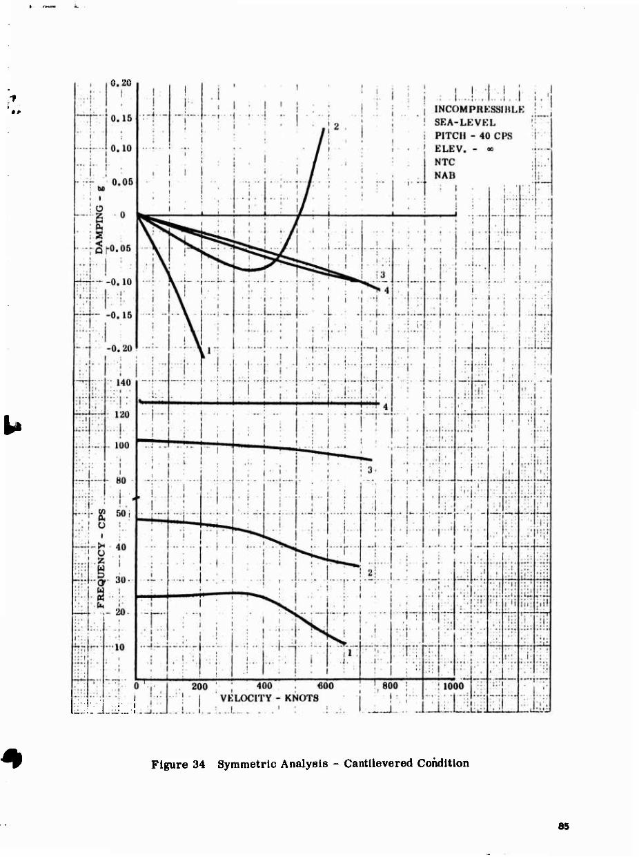
0.20
iL: 'U J_'J
Figure 34 Symmetric Analysis - Cantllevered Condition
85
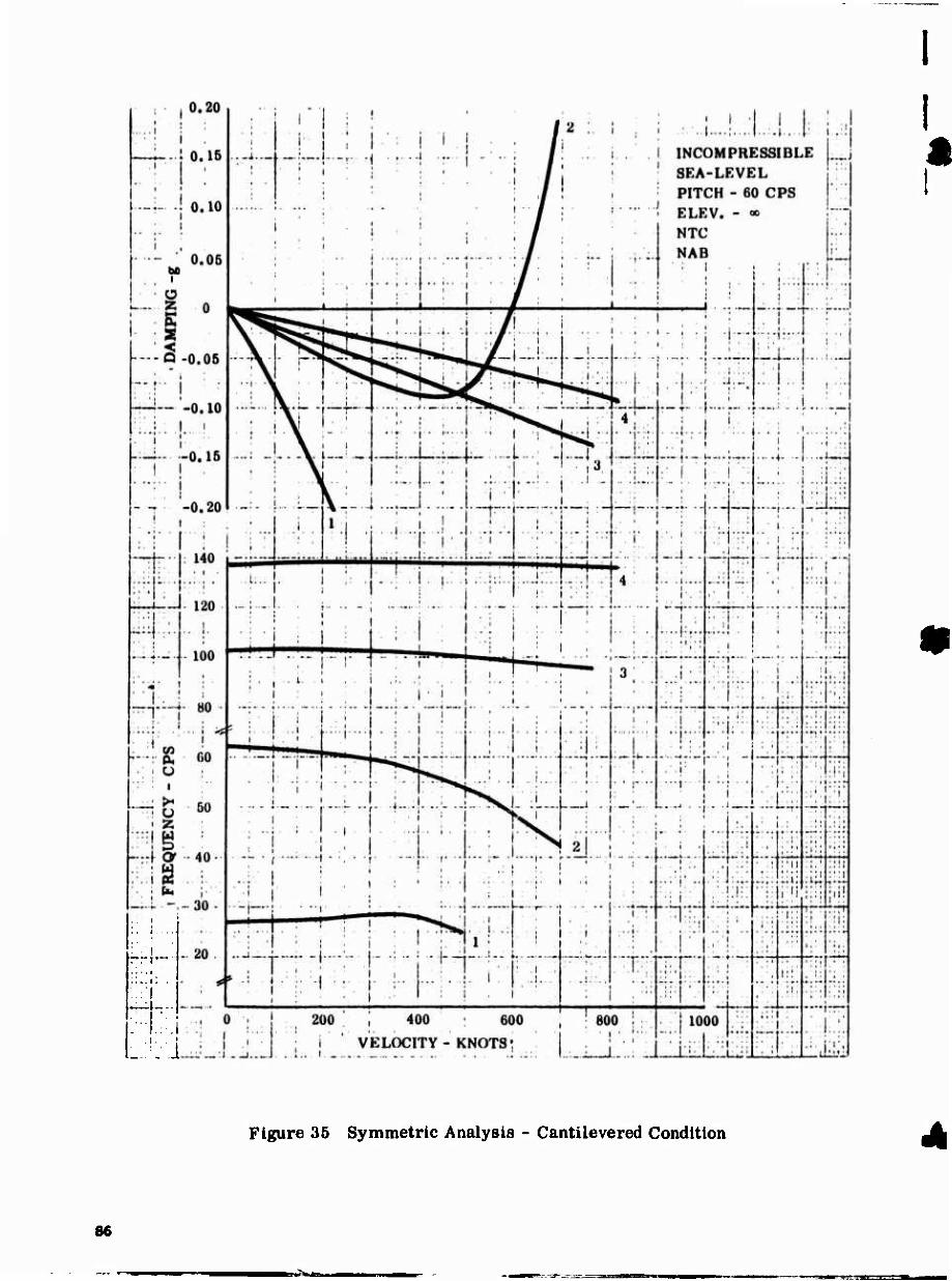
[rr-
• ■ ■ ■ i
.
(
1
Figure 35 Symmetric Analysis - Cantilevered Condition
86
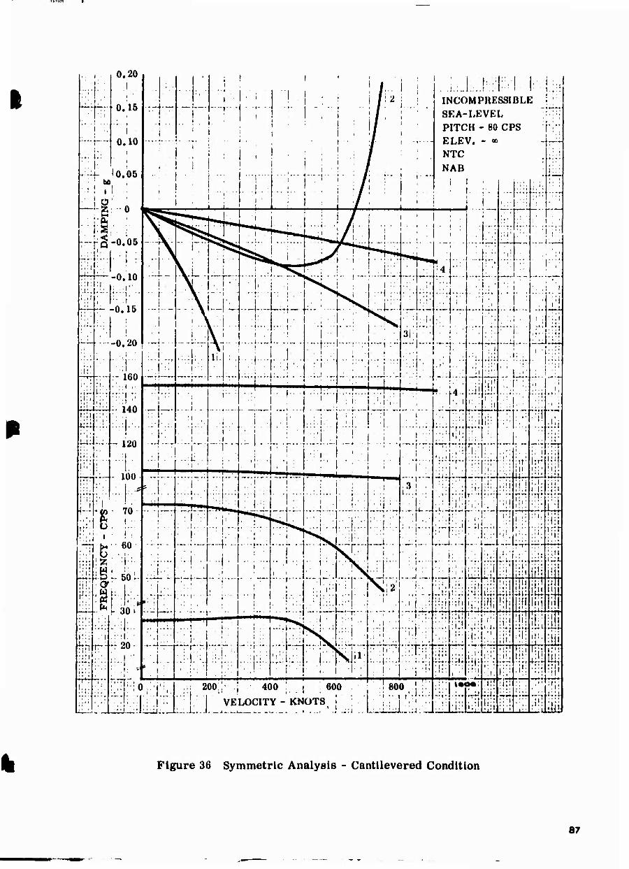
1 i ■
i: ■ 1 0* 20 i
i i
i 1 1 i
i i 1 i •
■ 1. !:.:• !;;. 1 i:., L-U-
0.15 ' i '■ 1 ■ ' ill:! ip : INCOMPRESSIBLE |
i I •' 1 . i ;/. : ■ SEA-LEVEL ;! M
i ":'. 1 ■
■ i ■ •
i ■■'■!■, i ■ ; ! : 1 ' ■ PITCH - 80 CPS ./,.
| 1
.; 1:
0.10 1
1
1
.-.i..,. i i . t ■ ■ 1 1 -,-•■-
; 1 ' j : | : ! ■ ; : 1 . / : : . •Ill ' ! 1 ,.!:/■ ;
ELEV. - * NTC
NAB 1 * ' ' u;..f iQJB •■ 1 • i •■ .... — • '-- -.---! : I' '- 1 i. ... : i "i : 1 , ' i .• 1
1 ■ ; i ■ : : /; i 11' i it. . ''■'■ '
U-!-g:..0 J 1 " i
i . i :/: ' : r: r .,:■
■- •;'' j
I'» i ':■.;;/, , , , T. r n ; a. ' 1 x "^te L 1 ' 'i „ Li 1 1 ' / 1 ' ' , ■ ■'' ;:;
1 ' ■ '
: ■ i:S;. ; \ ^s^Fr* ̂ " ! ' ' /'' , ■; 1 • • ■ ' : ■ ■•
,.... ::•■ '\"\''.\
H-rS-o.os A I^^I ^..TT^^Ult^ ; I Ml.
Hr.l... ■ 1 i i : :|> k ; ■ i ■
"•«^^^ii^x:;. . j j • -i^ h-: • .. .1 -:tjur ,.:;: .:. \:''"\ ;.:t ,
-0.10 i \L- — l;: .... .^S<^.-i.. ,...U:J.:.; —. ^.u 4 ...
r ,.,:L:T ' ■'l ■■
;-- -i;- .. j. . \ -'■I
r ■ ■"#'■>'
■1 ^VJ : , ..,:;, t (i
,:.:,].... - c- * ■ i
i '71
F~ [- -0.15 i
...;.-_ -\-d- :|; -.— .' i ->Ss|-:
■ ' : . .i.
i—j.-. i'';
... 4.... .;. .. i
1!' *' i
1
-0.20 !
,1 ■ t j
^-
i ....I
... 4 . • ♦
l ■ .....t,.:
...: ,.. ■
3i:r 1
'":\:v- i ..„q ... !•■
•jj
r-TT 11'.' i.
■ 'i ■■
- 160
; i
' I'' .1. \i
11.1 : !
■ :'! '■"
1 T i , ■■ ; 1 ! ' ;.i .■
; i :
i 'i;.::
;;. --- • r
_.,. _.,.._.._ -::iT::. .1
'III :.. .,.', .. ■ .■A.'.: . . 1 ; ■ : . ,..., ■..\:..l...i..:r~r~* K .4.. Jl ,ll' :;;;1,,:1 in* : 140
1
1 ' ' i t 1
.. ..j . L ... .-.. ■ ■' : | ' 1 : i [?:[■::. i
: , II ■ i 'I
C'.i Uiil
i • ..1 ,:: ■ ■
i • I i
i \ i: j ■ i i ■ i .,; 1 i , :
i
:■..: -jn !:| i;:
: ■':
• ■ 'ii ;!ii
|ii;:
- 120 ..J ... : ' i
..:L .
1 ■*■■]'•;
'i
■
• 1 :
.J. Ü Jt ! . ! . .
,M,}.: .j : k 4
1 r ■ s 1! i ■
it1,
II
I i
hr-:
i!;i
lii J iii!
1 ' ' - 1 ÜU ...... ,
' ,1 . :-:p- ...... .
. j ~'T'.' i ! ■; r • • .: • i. • 1 !
, -■■•)■■-
3 i i . ; .. i
. i : i:
i '■ ■ :!!
-4— ,ii ■ < * i :;;J
11.',: i < i ■
r1 :'i .. i 1
-r^
(:•••
pm^ ■;: 1
1 r ' - ■ . ....
■, ' 1 . ■' ■ 1
, i' T "
1 ( ' ... i ;ii
;,: 1! ■
'i, iiiU 'L- 70 .. .j _.. ~1
r:* i : ! : i ;
:.., i ... | ... i
' ■ i
■:■}■■.■ :;-p:i| - 'I}--' ■ i
i ■. '.. 11.
:l:i
rr60 ...... , -4 - 1 "T " -^N^rr:- 1 ...
i
—,.-.. , i
... i -—' ■-■r-' -r-p* ~- :;,ii|
::: :S :l: :..) .. . ..| . 1 • ■ .. i.. •■ i •. V ... ... ... — -. ►.! •■.( ►w. i«J " i aIMoi ■ .■}■■'■]
■ i !
: ■' ■ i
. i I
; - l
i i
- r—
■!■■ ' % .' 1 ;;,
1 —,1 :■
1 •
:,i •41r IT
;:i
TTi i.'i .u;:
ill
f lii 1 fn
1 H ... 4....
tit Hi "ii ■ • ■
.' I
H 30 U
'■•:i; ■ •r 20
.. _ —,. - ■'.■ -i ! -i —•-—
' - ■ 1
■•■I
' ,i ■ ■
'^''-
TiT] •il!l
, . 1
t . . t . .
nil >* • ■ ■ ( ! i ' . i
li.
1 il;
UL, ii:.
i 1
M ■-••]
.,; i , ! "^Hv rr'H
J - —r-r-~l
■.::,i ;- ■ :i ; •
--:■. ^
. I./ S i '■'■■\ :i; • • t • . ill —H—rr
lit:i;; in Liii '".\
m ~"
1 '1 f 1 ^ 1 ! ! ■
'•■ ! : ■ 1 • ■ V i 1 ■ ■j ■!• ;!;: Ml, :i, ;:: if; I ' 1 ii!
i';;I li i''i :', 1 ;; 200: ; 400 : i eoo ' .! BOO ' !: ■■:.:\y~: i;! ii! ;. ■
. ' ' ,1! J < ■ ■ «1
■L : ;i : :: ■■I'l.i i . . .; ... , ,•.!...: -:;.] ;..i .i. »—.-,. * • >•{
;''] i. VELOCITY - KNOTS i : !:| ::; .-.1 'ii ; :i il: M .j~'.! .••! :' ' ■' I .. 1 ;.:. ... 1 _j i . ,.. _; .. ,.;.x:^J __.;J :_J •, 1 I;. ^.'i. ~c\. ..i,,:. .j- ■ .L
Figure 36 Symmetric Analysis - Cantilevered Condition
87
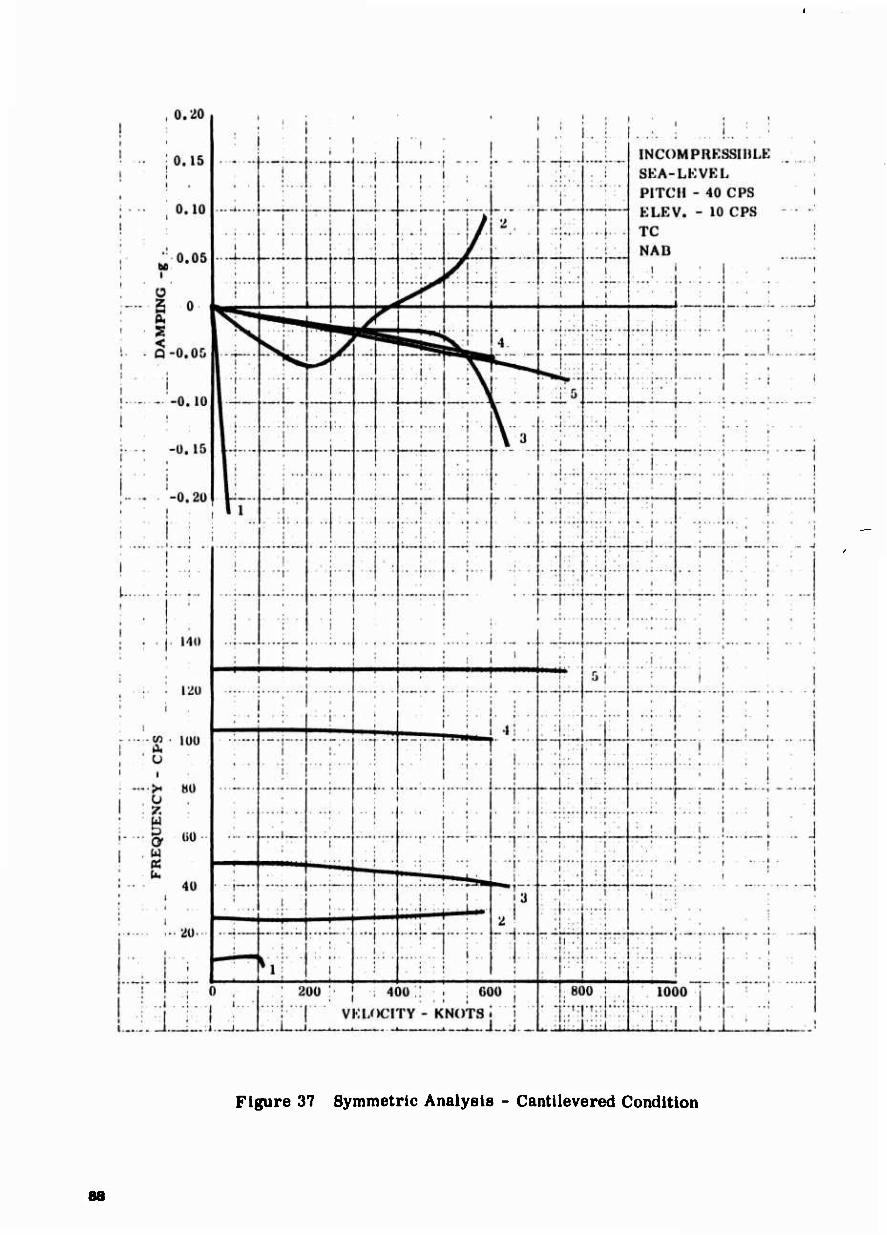
Figure 37 Symmetric Analysis - Cantilevered Condition
88
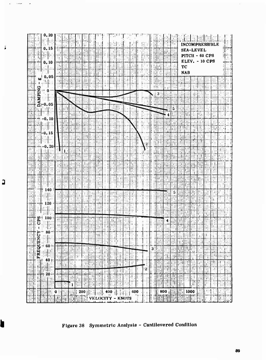
0.20 , .i;
ili
ilii
II; 0
i:;.
i:
u-;
200
M] : •Ti VF
Ti:~
400
LOCITY - KNOTS JL.J.
•vi:i; ii; I:;
iUU;
: 800 j
Mi ffn 1|U
HÜ tf.t ir|T
1000
III Ilii
ili It,!
Lüir-
:,l^ u:; ^il-illililii iiüh: INCOMPRESSIBLE SEA-LEVEL PITCH - 60 CPS ELEV. - 10 CPS TC NAB
Figure 38 Symmetric Analysis - Cantllevered Condition
69
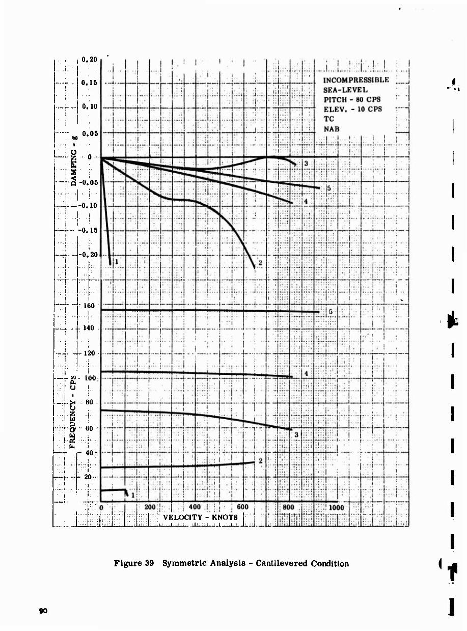
bfi
0.20
0.15
0.10
0.05
L.IS
■L2 •0.06
-|-—0.10
1 -0. 15
!.
--1- - . . 1 .
■'!
-0.
—
20
I 1
- 160 i
-.1**. *..
j.
: 140
i i
- 1 20r
.*. to ; ^ o
■ll
100; I
80
60
— t-
- 40;
i 20-
i ■
L.iM . ; 6oo
: VELOCITY - KNOTS I
Figure 39 Symmetric Analysis - Cantilevered Condition
90 1
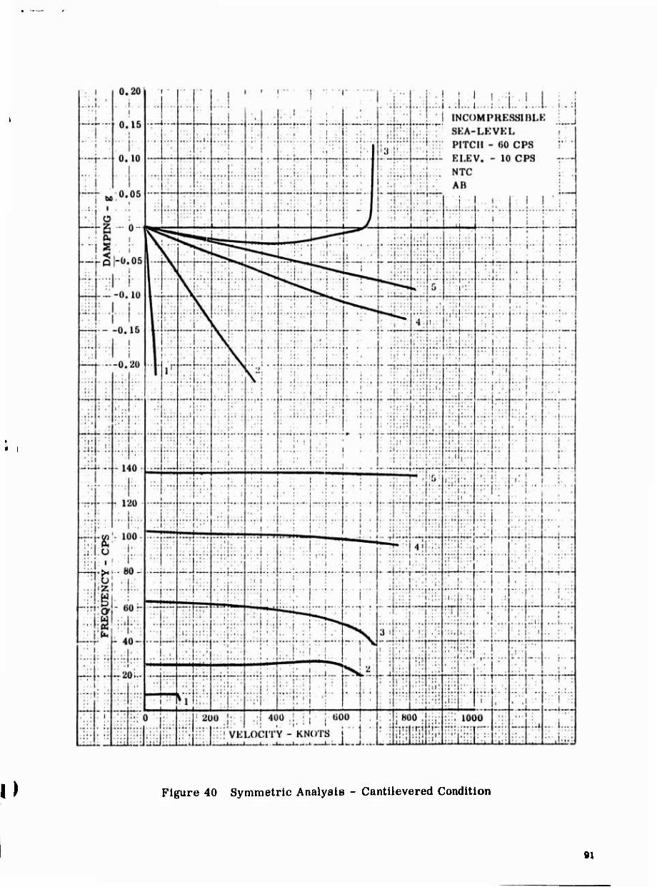
Figure 40 Symmetric Analysis - Cantllevered Condition
91
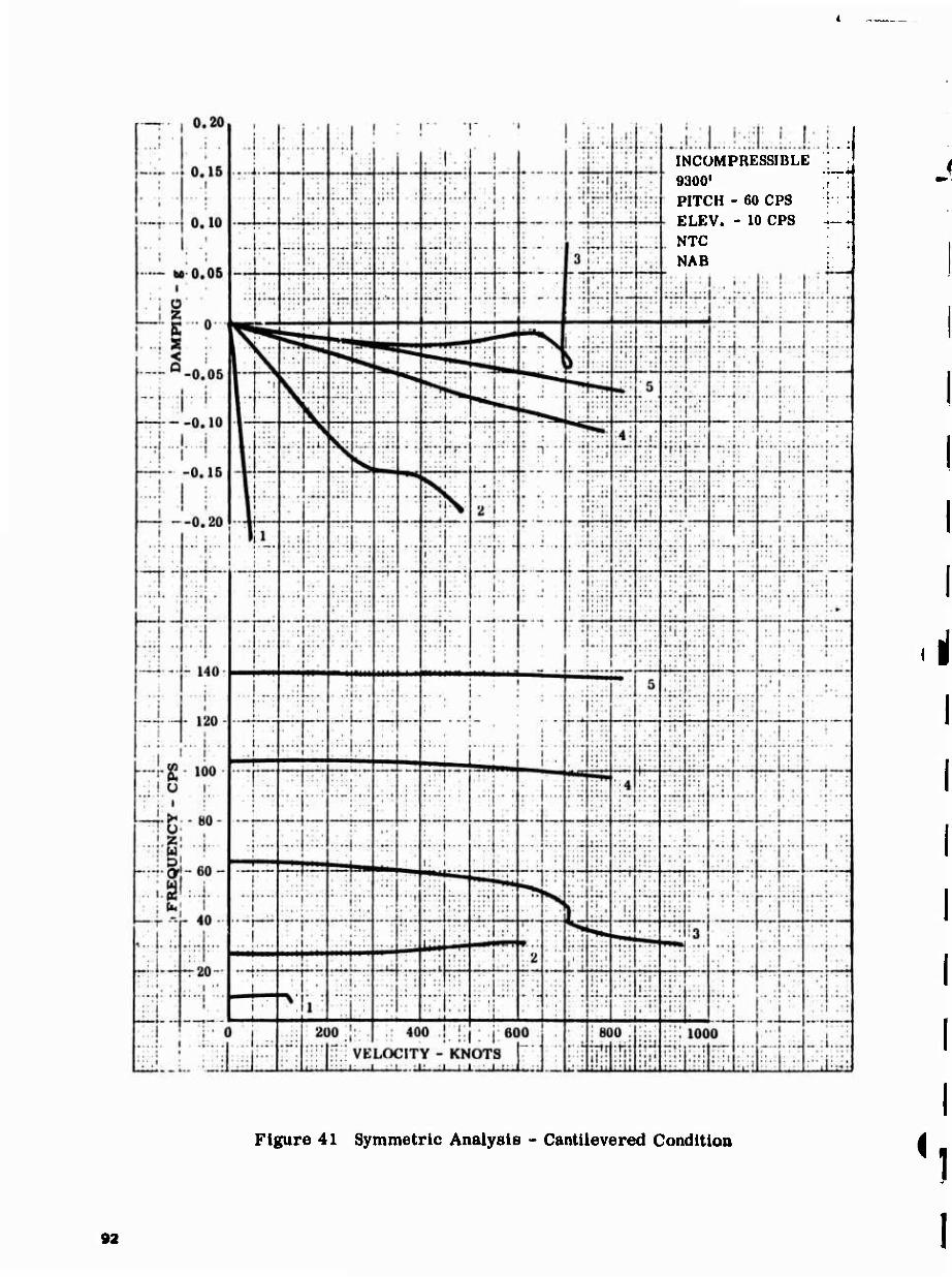
INCOMPRESSIBLE 9300' :J PITCH - 60 CPS ELEV. - 10 CPS NTC NAB
Figure 41 Symmetric Analysis - Cantilevered Condition i
92
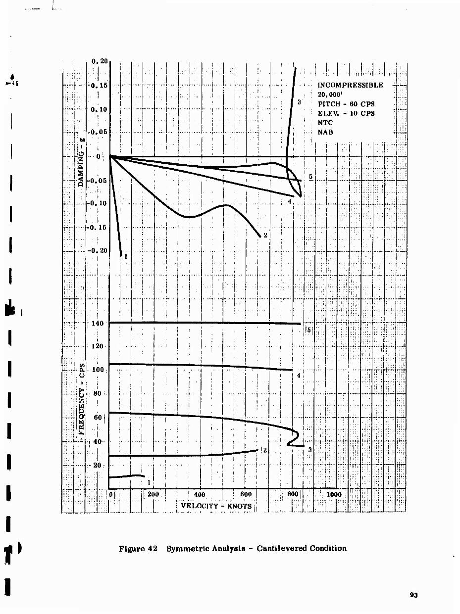
L.
-^l
1 0' 20 i 1 1 ' i 1 1 i t 1 ■ 1 ' 1
■ ■,
i
1. ' ' i ■ :.| 1 i,l.::. „l;|;r; ; ;;
1 1 •0.15
r ' . ,...i 1 1 1
- j ' ■ INCOMPRESSIBLE r
' J ! ; 20,000' MI»*J
1! r: ■ , ' i 1
,1 ,. ■ i ■
1 ' ' .1.
(*■ • * 1 |!!. 0.10
■ ■
I ... .i. .; ■1
.. . 1 .. i 1 3 PITCH - 60 CPS '
1' 1 1 . ., ...
i i j : ELEV. - 10 CPS
i i •■ • i i i . 1 : / | NTC
L^... -. ■ 0.05 1 1
.... ; -■ •• t *'*
....u.. .. i j', ;..; NAB !il
- bfi ' 1 ' 1 ■ ■ 1 1 i i
1..' ü ii
1 -■o ,
I 1 : 1
' 1 1 I I i rl v
"*" \"^ ^-..
• •''
1 * 'H
' '' ^^^^^^ — ; ' ——^-^J 1 i 1 1
1
\ **,***,*<«^IIL" - — 1 1\ . I •;'' ■ 'i
1 '' i 1
-0.05
I ^■0 10
I . TV ^^^*^^ r-^r-rr !.-.._ • ♦- •■
rHT 1 ' ] *
V; |\i ■
1 I
1 i
; > V 1 ; ... . 14. ..] 'I' \- ■ 11:' :':
rr-
1
i
-0.15| \
...... . i .........
, j
< "Hi:: i
i 1 ■
i.;.. .:.;
1'' ::::
' 1': .II
1
1 ' • l
-0.20 \ j
i ....
i \2 i
1' 1
:.,; i ! 1
1 ;
■;:
. 1
1—'
; ■
in
11 ; J.
■
i
.....
' '
'
•i
• ....
....
■ !■
. i
"T : ■ \ .
. i ' ... j. ,
i
1
■ 1
. 1
1
1 ........
:
....
1
i ■ 1 <
■;i;
1 ■ *
..... . . ■
: 1
. -»■
.1''
1 ,
; f
i !:
i— ■:~ ',
•
, 1
■ ;
—- 1
i140
i
; "" —
i
i 1 ■
I
"" "5J , ^
i ;
trr : 1: ! 1.
1 .:
'■ •
rrr ' ' ' 1 .4X1
1: tn
; 120
■ ■ !
J . ■. 1 i
. i i. . .
: 1 !
i 1 ;
i ' 1 1 ! ! I
...;. Tft' r4- i 1
*T *— i
: 'H 1 ■ i 1 , ■
■fil.. 100
! ' 1 ' i •ß- 80 ;.
1 ,. !.. ■ i ■
i i
.4
1
. 1
| 1
1
... | .
4!
...,(
' nr fi- rl j] 1 :! i ' :'l
■M\ i ; ■ ; 1
i
1 1 1 ; : '\
ig! : cy; 601
1 ■ ... 1 j ,
: 1 ,
. 1 1
. j 1
.. I. . • 1
1
■ :':
, , 1 .. 1
1 J
1 :
~M ... , . .,; ■ i ,"""^"*"**"—"^^
a i i I
i i 1
i 1 . I.I Ifc^ i V'l . :
'• '•■\
, .. * I 1 • | I [J
n 1 ' i < 1
11 , 1 ̂ ' .I1 ■ : ■ 1 ,'•
: 1' 1 :; ; ;i 1 '. ;|
L-.l * — ,40 .. .; , , • r | '! 'I -'•^[ *-H • r Hr rrr t^i -^ir* "* *H i^
r ■ ;.:. t 1 i .: ^73
t' 1 1,1
■ ii' M!1
1 :: ( . ■ 1
■ ü ill.
' 'i
! i: • • ■ • •
1 * l • 'rl , . •2 : ! . ! i 1 1 1 1 . .i. .,
::i '■
\: ■'] Ü • 1 ■_J i
■; ■ j
i i . ■ ■! .
..;. ' : i'
1 1, ; 1 1
1 ;
: .1
W; H : ;. .' ' ' , 1 —J i ., i ■ 1 . ., -J
i 1 1 _J -J 1 ' ■ 1 1 ■:
1 r
1;;' ' ' ; '
• • ' '■ •MO ! ] j 200, } 1 ! 400 i 600 j ' ■: i 800ll ,*!; 1000 : i 1.
; i! : 1;
.., . , : ..[ i' VELOCITY - • KNOTSh \
. ... 1! _J :LI i n „ -i. J ■
■';:! '. jr I; ' 1 1
;'IT
■ ■
1
' ':
Figure 42 Symmetric Analysis - Cantilevered Condition
93

. 0.20
Figure 43 Symmetric Analysis - Cantilevered Condition
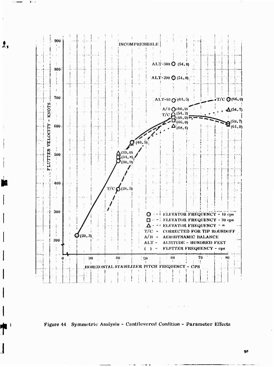
i
9ÜÜ
L .
■
»- ■
i—...
r * ■
r .
. ....
....
800
700
h O
£ 600
i
K W 500
400
300
200
ALT-MO O (^.b)
ALT-200 0(51.8);
(
■ :■ ■
1 . .
); 1 ;
■ t • ■
; :io
,non
...J. 1
ALT-;i:{Qi(44.5)
I i
A/Il<*)'4ü'm
T/cQ^54-2) "^ (40.0)-.— — S^-^^
(40.0) .^^ "'(48.4)
l0^*T/C 0(00.0) 1 ; j '. , ^(54.7)
i(5y.7) '(01.0)
I KLKVATOH FIIEQUENCY - 10 q»« I KI.KVATOlt PUKQUENCY - :iü cp« i Kl.KVATOH FHEQUENCY " *
CORIU'X'TED FOU TIP UOUNDOPF AKHODYNAMIC UALANCE AI/mUDF - ilUNDUEl) FEET I'lAITTEU FIIEQUENCY - cps
4- 00
i I
lUmiZONTALSTAhlUZKIl PITCH FHKQUKNCY - CPS iii.1
70 • i
i i l i i
80 I I
I
L._l .
Figure 44 Symmetric Analyaia - Cantileveretl Condition - Parameter Effects
9F
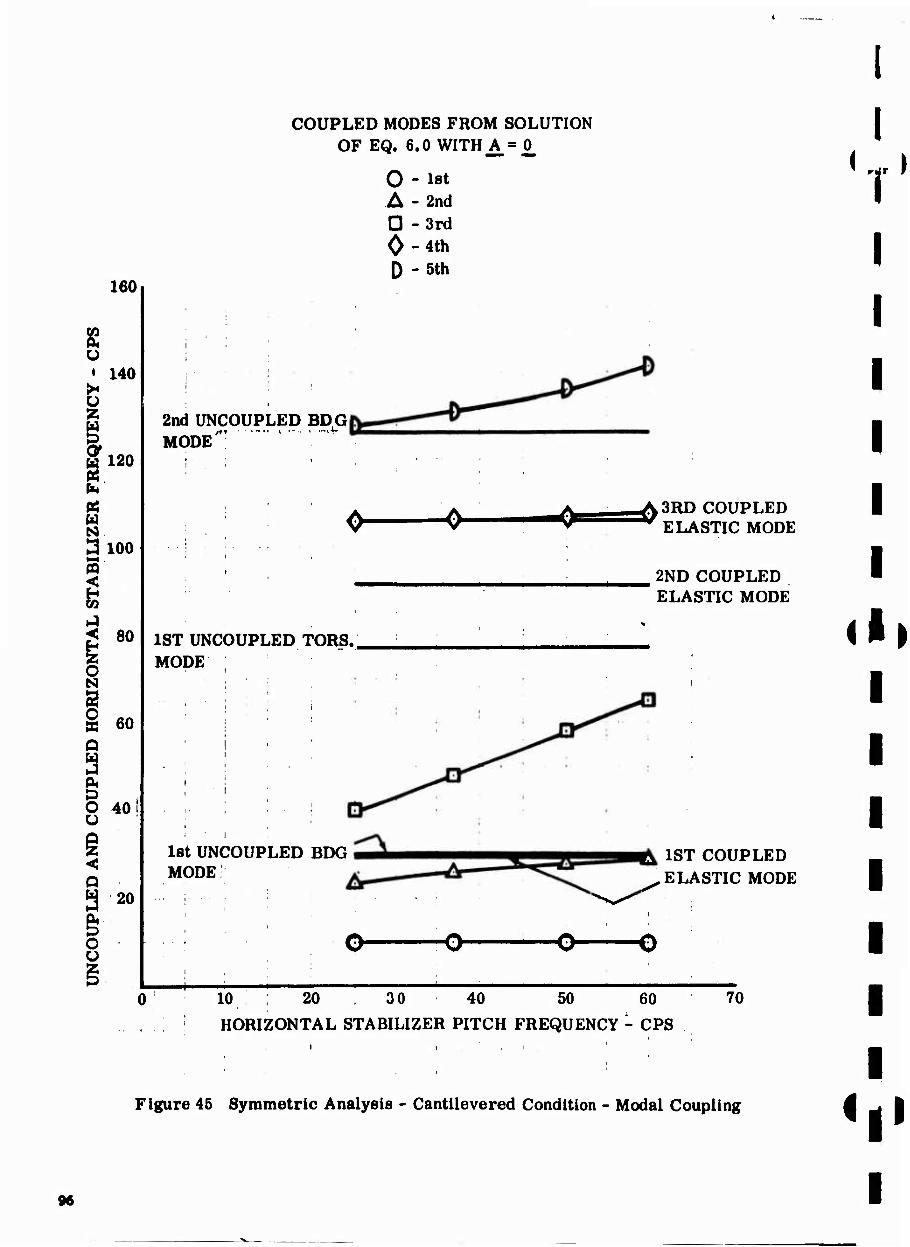
160
s ü
• 140
B
I U 120
M N 13 loo a
< 80
O
i S 60
P O 40 U
< Q a O
20
COUPLED MODES FROM SOLUTION OF EQ. 6.0 WITH A^O^
O - 1st A - 2nd D -3rd 0 -4th D - 5th
2nd UNCOUPLED BDG MODE
1ST UNCOUPLED TORS.. MODE
1st UNCOUPLED BDG MODE
S3RD COUPLED ELASTIC MODE
2ND COUPLED ELASTIC MODE
|^ 1ST COUPLED ELASTIC MODE
10 ; 20 , 30 40 50 60
HORIZONTAL STABILIZER PITCH FREQUENCY - CPS
70
*..
I I
i
Figure 45 Symmetric Analysis - Cantilevered Condition - Modal Coupling i
96
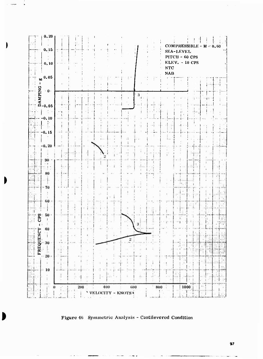
0.20
. 1 ■ 0.15
1
0.10
' ^0.05
. ! • Ü r-
■ ; s -: Q-0.05
■ • ■ i . 1. I .
-0.10 i r
:;t. — -0.15
I I
■' -1
1 I'll, II' ill
COMPRESSIBLE - M - 0.00 SEA-LEVEL PITCH - (JO CPS ELEV. - 10 CPS NTC NAB
:i
— ; — ■-• i
I -i • ■! :■ .1 1..! i ' 1
r-
.1...
Figure 46 Symmetric Analysis - Cantilevered Condition
97
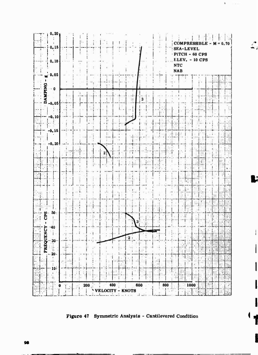
I .
0.20
0.16
0.10
0.05
s ■ a
1
i
-t ■ - I
•0.05
-0.10 ■ i i
-0.15
-0.20
m
i- ■
I u 50
i
40
30 ■ i
I—H- ,-20-
MI'.
H
- 10i
! ,;.:'.
—:.
I...-. i
i 400 ; ; 600 VELOCITY - KNOTS
Figure 47 Symmetric Analysis - Cantilevered Condition
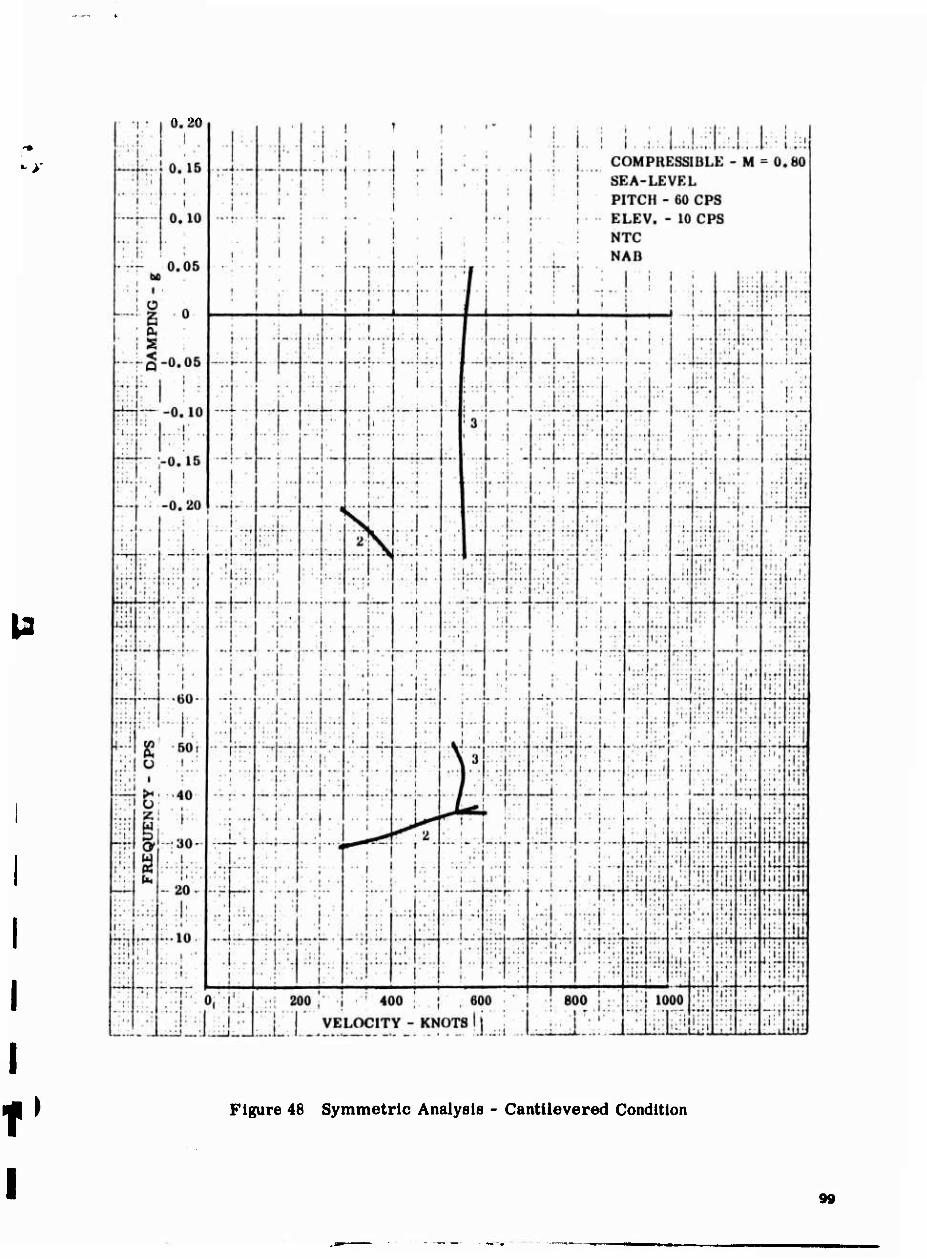
0.20
Figure 48 Symmetric Analysis - Cantilevered Condition
99
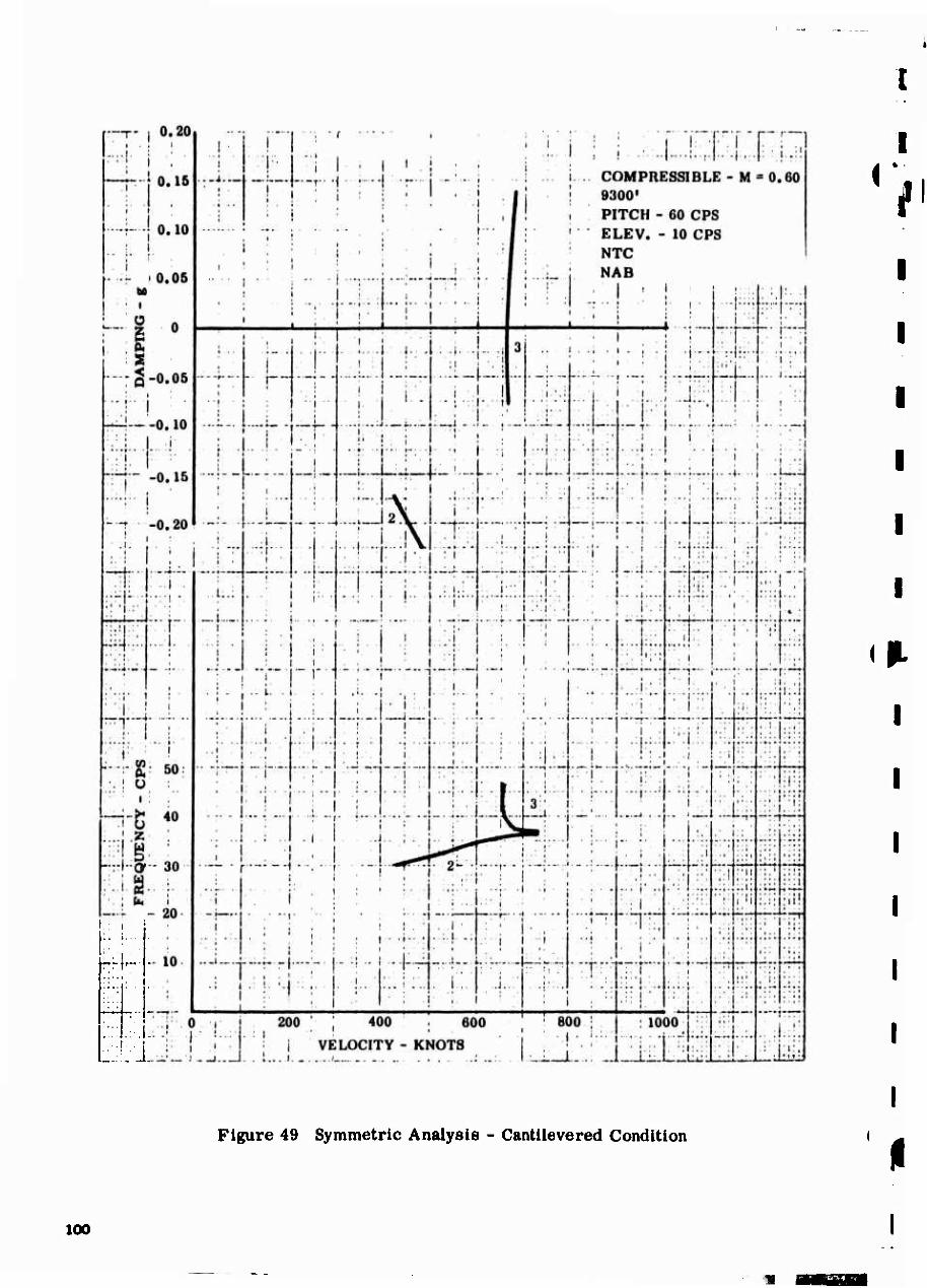
1 :
1
' ' 1
Figure 49 Symmetric Analysis - Cantilevered Condition
100
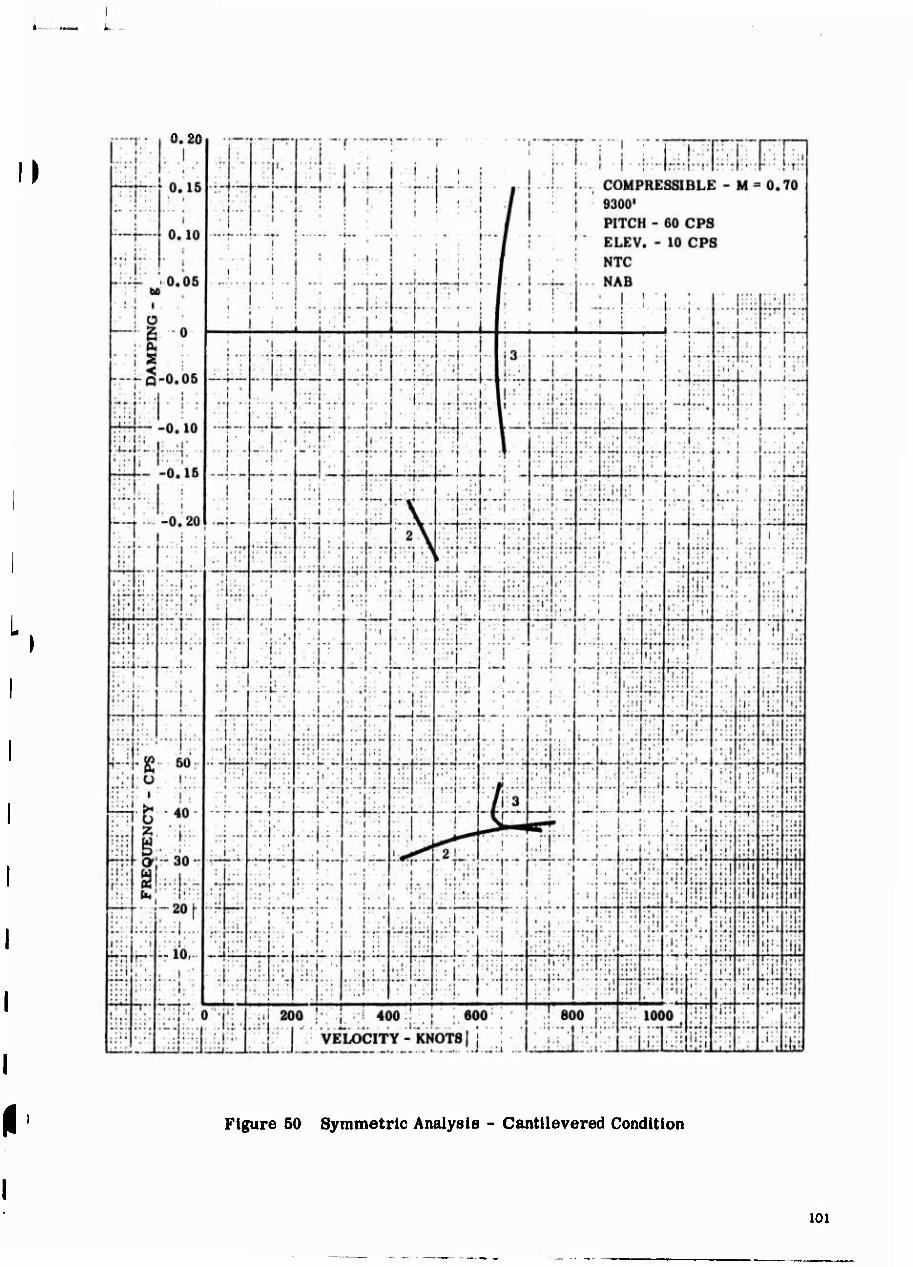
0.20 -
Figure 50 Symmetric Analysis - Cantllevered Condition
101
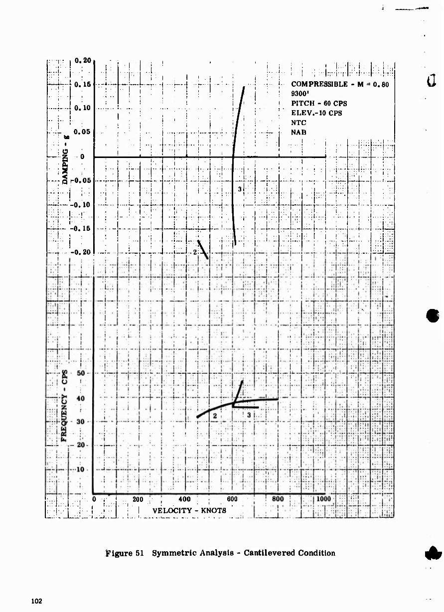
0.20
~p-'0.15
0.10
- 0.05
■; • 1 s Ä ,g o
la ;• -S r0,06
-: 0.10
;i::.M:-.. 4 0.15
~-t -0.20
i l M—i r-
^ ■■)•■]■
j COMPRESSIBLE - M = 0.80 I 9300* ! PITCH - 60 OPS ! ELEV.-10 CPS
NTC NAB
■; i
.;. L.L-,-.--J...U-U:VI
::..::i.:.,,:
! t
\ :-.|.
;._j
r !
\
i
t •
» ■.
I .l-._
• i ■«
• i
i
:;<.-. .LI.: .1;...;. ■ ■ ' ! ' i 1 ' ' j ' I „.|^_ i—•.._ .\—j .;-f4r-
:;-i .■-■■ i VE __■„. ■l.-:_l.._J.. ..1... i. _... -...
200 :■ ; 4oo 6oo VELOCITY - KNOTS
Figure 51 Symmetric Analysis - Cantilevered Condition
102
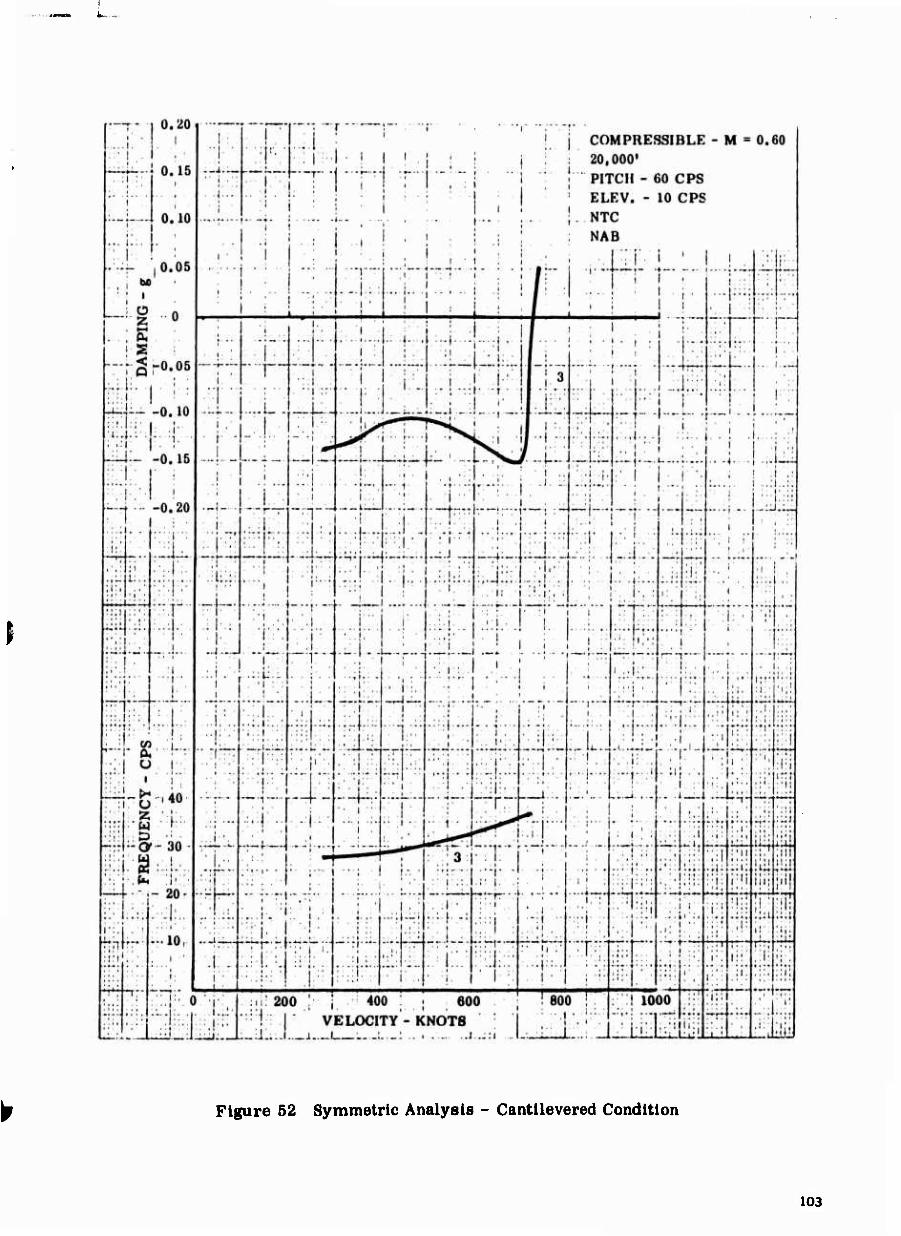
Figure 52 Symmetric Analysis - Cantilevered Condition
103
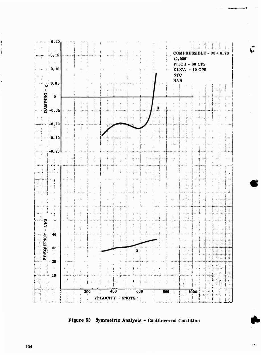
0.20
- 10.15
0.10
i
Ü
S s < Q
0.05
-0.05
— •- 1-0.10
L.J... -0.15
-0.20
...i: . .
J i
V) 0, O
■>
u w
40
30
20
10
:_U.
I I ■!
COMI'RESSIBLE 20,000* PITCH - 60 CPS ELEV. - 10 CPS NTC NAB
0.70
r -r : ' i. . . .1. .1..
200 400 600
VELOCITY - KNOTS .1.. ...J
800
...J..'
1000
. 1 :'
:t
i.;,
Figure 53 Symmetric Analysis - Cantllevered Condition
104
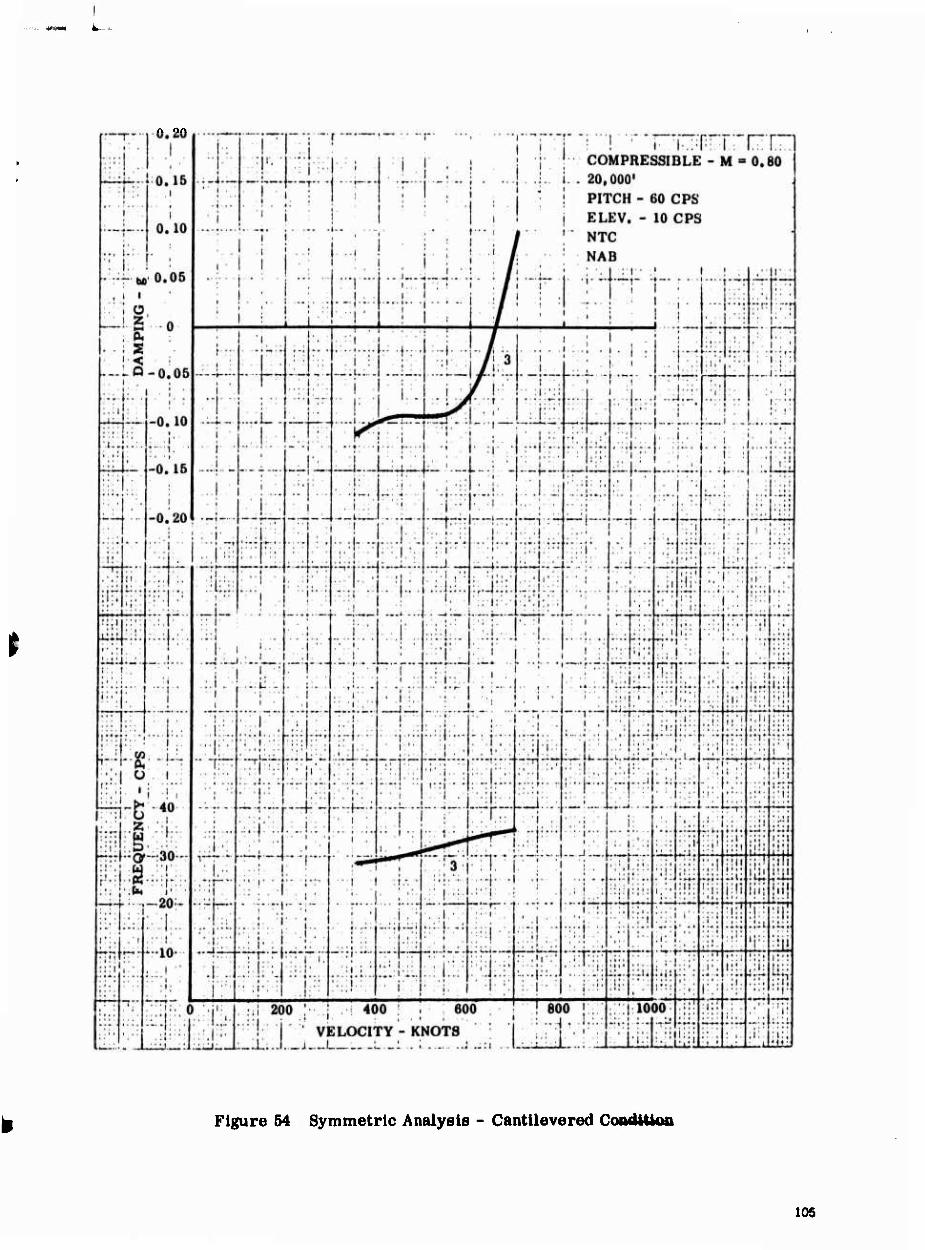
0,20
Figure 54 Symmetric Analysis - Cantllevered Condtttoo
105
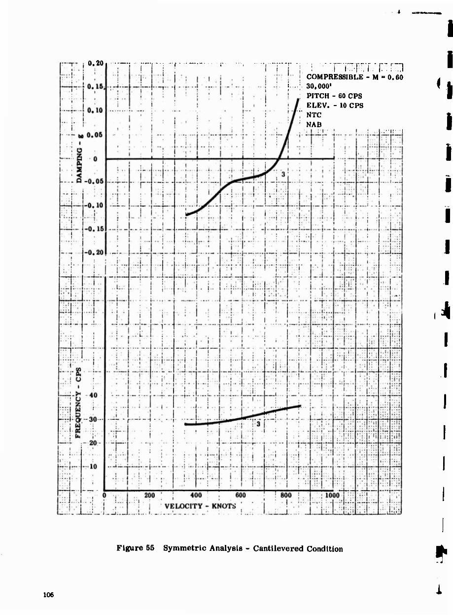
0.20 —
COMPRESSIBLE - M = 0.60 ;....;. SO.OOO1
PITCH - 60 CPS ELEV. - 10 CPS
T NTC NAB
.,"lr
Figure 55 Symmetric Analysis - Cantiievered Condition
106
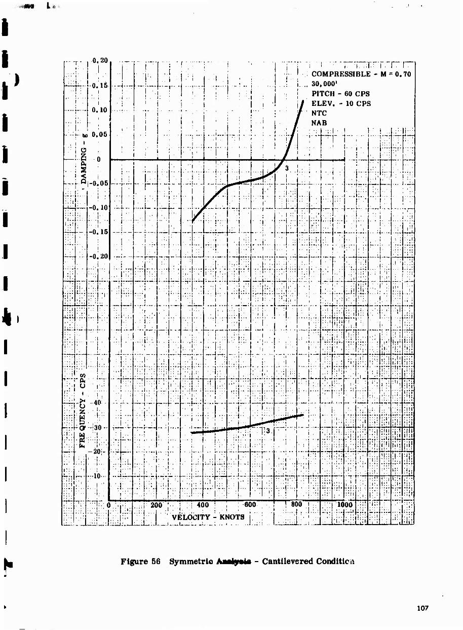
*
)
n.20 ... .
.■;' i ■ J,. 1 ' if.; i
•■h- Mi i •-. i . j : 1 i. I,.:!:: 1 j ' COMPRESSIBLE - M-
11. 0.70
Lili:' 1 A IR 1
■{ • ■
; .. , ■ ■
' ! ■ i : . 30.000* 1
! •!■ : ; ! : j '! PITCH - 60 CPS
•--•--- 1
0.10 1 i i ■ 1 1 ! : ■ 1 ! .
i ! j / ELEV. - 10 CPS ; / NTC
... ! i
i ■ 1 1 i : 1 ! 1 ' i i i ■: , / NAB • r to 0.05 ■: j •: i ..., ... 1-4--!. .1. : .\..:U ■;:l ■ .!
i ■■'
:— ^
:: 1 o . ..!...: i . # !
1 1- I-. :;;. ~Tr ;■:
„!.2 o . ■ a
1 1 : i i , I I ■ 1 : ! # . ■ l rrr —- J. 1
: 1 1 ■
■... i . i : Jr " . 1 ■ . .1 ■
• ~
•2 1-0.05 i
■ i :
-A in
-, . - - i 1 'J #
I
; I
^ ! ■ i .
■
T ■
1"
i i
! . ;!:!:: :: i:T,:
:_L' •
.;;...
l
■ I ■ ; .
-•• . i
— ■ ! i':
i
■ .1 ' ■■ i ■ :' 1 :
■. :
1 i
I.::
T 1:;
L
.1'.
-0.
-0,
• . ■•
15
20
i ■■ . j.....
■ t
. «1 - -■
,' 1 ... h:'
.
—r
; ■ /
:: U,.J
i
•i-lr:: ■ ■ ( •
..•i ■
:;1
■ •
•
■
■
■i;
i —
• 'j: ; i
: : 1 ■ ■.
' i ::'
i'.:
. . -
• 1
-~-
■ •
- —.•4.
. ■
• , i
• • •• • i
■' r.; •
. <
■ t
'.". i :i:
, i • •
:( ' ■ .:'
■■.:■.
ii. i;..
;"; 11 •
..,. ■ ■ j
.I:!-.:. 1:
.:.L: 1
.i
■ ■)
, i ■
I
"T .
■ ::!' .j:..; 1 ■'
71 1
J. .■1;:.
1 .».i ... ..: _*;_:
m .: 1; .■
,...;
,:;!lr:;
.-:.!:■..■ •, ■ i ■ •
•:!:!■'
■ i , 1 .. ■,
. ■ .
i! .
.:,T :.
■ i".
ii. .,:■
'V1 ;: ■ i
;■
-:-!•■•
. :T;"; - 1 •
i.;,
1 ...., . t
: t ■
i ; ■
t t
: ' I ■ ...... i ■
..1 IM i::
■;
■ t ■
■
I1
ii: !i;
• ! : +1, ..' '.':'.', :: i
lnJ
';■"
• •• r ;::
: 1 . .:„1:.:.
1 .. i ■ ■ ■ • 1 | ..
i
* . » - . . *
. ] • i;.. . • ,♦•
■ i:
.71 i: ■::|::;:
':"■
i: :
i.li
•rr i • i '
.■ i CO ■ !
i ...
... I. ..
"~r ?;--,- ; ■.': ;:, ■
V:
- * " : .
'':'■•;
— •.. - • i _
rv ;r:|.,r- ••■ !;; : "I1
, ■!; !:■
■::,i;; .
-M i ;:
MI; •in K;I-
m-™- -~-1 — -'- r.^;: 1 .
" "T " l~ li^'i: [....
i ^, i., .- .. '.i'üi. ..;. Tf iuf
; t
z ■ ■..
-Cy -:30-
■ ■ 1
:■' i■ • ■
. i i "
i.
■
1 • ' 1 ^p
**f! i.
1:
iiii ii': 1
i i
■ ;t.-. •
:1;3, • : ■ ...j. . .; .
< i. :;;! tin * • t • iül ' Ii
l!|l
fe 1" : OA' ■ i • ■ [■ .;:' j: ... ■ ; 1
1 .:: ■ ■ I'.! 1." • • i . !;i; i:fi
lit. III! i"!
1':. f ■
. ' (
i
-10 • 1 " — 1
M ■ 1
:;•.
..........
. ■ ' * ' ■
i.. ■ .i.
1
i ;; -."• '-:':
. .i •:
1 i '
:'''',,
■!; i
. : " :
. I:'!
1 1 .
. :. • 11 •
...k'':»
i.'l "
[ill Mi: |; i::
ii'!
ii,.
iiii 1'-
■ J. .. 1 ■■
... ... ::.!■ ..'.''{'.:.'.. •♦»■ i'1; i. |
, I •
:■ .[r:'
i i
',1t t
;ii; I'll '.':
: i:. !::i 1:'::
l;|i 'ill '/I-:« .:r:. ;! 200 ; r i 4oo i ; eoo i ! soo i ; | 1000
;!" ( . . , -mm •:H.: •
i VELOCITY - KNOTS ! 1 ill :.; i
■1 !
* •" .i:. i ii^
Figure 56 Symmetric - Cantiievered Conditica
107
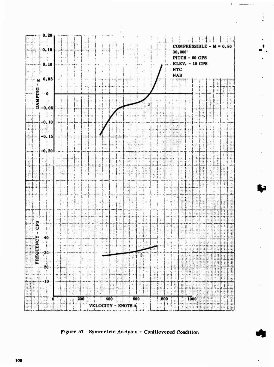
Figure 57 Symmetric Analysis - Cantilevered Condition ^fe
108
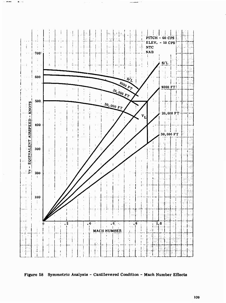
700'
600
Q W w
< H Z w
5 <y u
>
500:
400
300
200
! 100
■ I..-
i ' i
i . 1 1
1 I 1- ■ 1 ■
1 •;• Li !.,. ,. y...
1 i i
• ■»•
i'
1 I- :
! PITCH
• 1" 1 .! 1
-60 CPS
: 1 i ' ■
1
...
1
i
i • ■ .!
,. .,.,..
■ l
• I ■
i . . t . M.,
...!. '. i " j" ELEV. - 10 CPS
■ : NTC • ■
^^-♦* i-»r*«4
1 \... i ... i
,....j..- | ... 1 .. i ■ .,^ NAB
1 ■'■
i
1 ' ■ i
• t •- •
i 1
1 1
1
: j • ■ ■ ■ -t - ■■
i ■
i ] i--
i .:. ' 1 i. |... i \J.S/.k.\..
■
f~** •
• ^"^^^ o!^^^' :./-
... ! ,...
' ! ■
..i . • I
1 1 u^r^> /
/
L 9300 FT
t •
1 1
■
■
1 1
,.. "^"T^^-^Opy r -/
1
t
! :!,r7> 61 K .20,000 FT:
■ • ,1 ■ i . .
I ... ....
1 ■ 1 :
// /
i • !• 1 -1 •■ ,30,000 FT
■: :
' : • 1
■
7/ / ^r i
i
i
■
. . . • ■
:
^
/ J
r
/
/
/
•
i
i
■ •
i
r • ,
!
■!
j...
i
i..
. I:,
— • —
" '
■ I ,..( .
.....1 .. i
i
i i . *
..
.. ,. j
r ....
i . t
/rl i
•
;
—j....,
!
i t — r. .
■ i
!■ 1 i
i i
I ;; ■-•-i —■
t 1 i .. | .
1:
-r- r-
' 1 ... 1 , :
-i ''. i . ; . 1 1
:—' '\
> ' ; .2 , i . . i !. i : 1 .
.4 i
: .6! ■. I.I
i '• B : i
1.0
: i ■
: ... . ,
t
' 1 "• t
i ..I.. ,
\
I
i
i
i i
J .1
. . . , . ., MAC H NUK i
■
i
IBER
i
■ T ...J J
i
i
i
i i ■ ■
i
i; ■■ r
: i
'" 1
-1 ' <
i ' '
Figure 58 Symmetric Analysis - Cantilevered Condition - Mach Number Effects
109
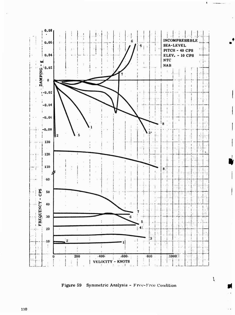
0.08
0.06
I \ 0.04
bfil I
Ü s s
0.02
«-0.02
-0.04
-0.0«
-0.08
i i : no
— 1., 1 GO
; (A ... . f^. bü 1 U
i
o 40 z w
: D . .; O'; ao . ;S:
1 w i
20
.--i-
1 ! i
i
... i. .
, .. i
..... i
... ., ..
7 /
i
Figure 59 Symmetric Analysis - Frt'c-Frce Coiulition
no
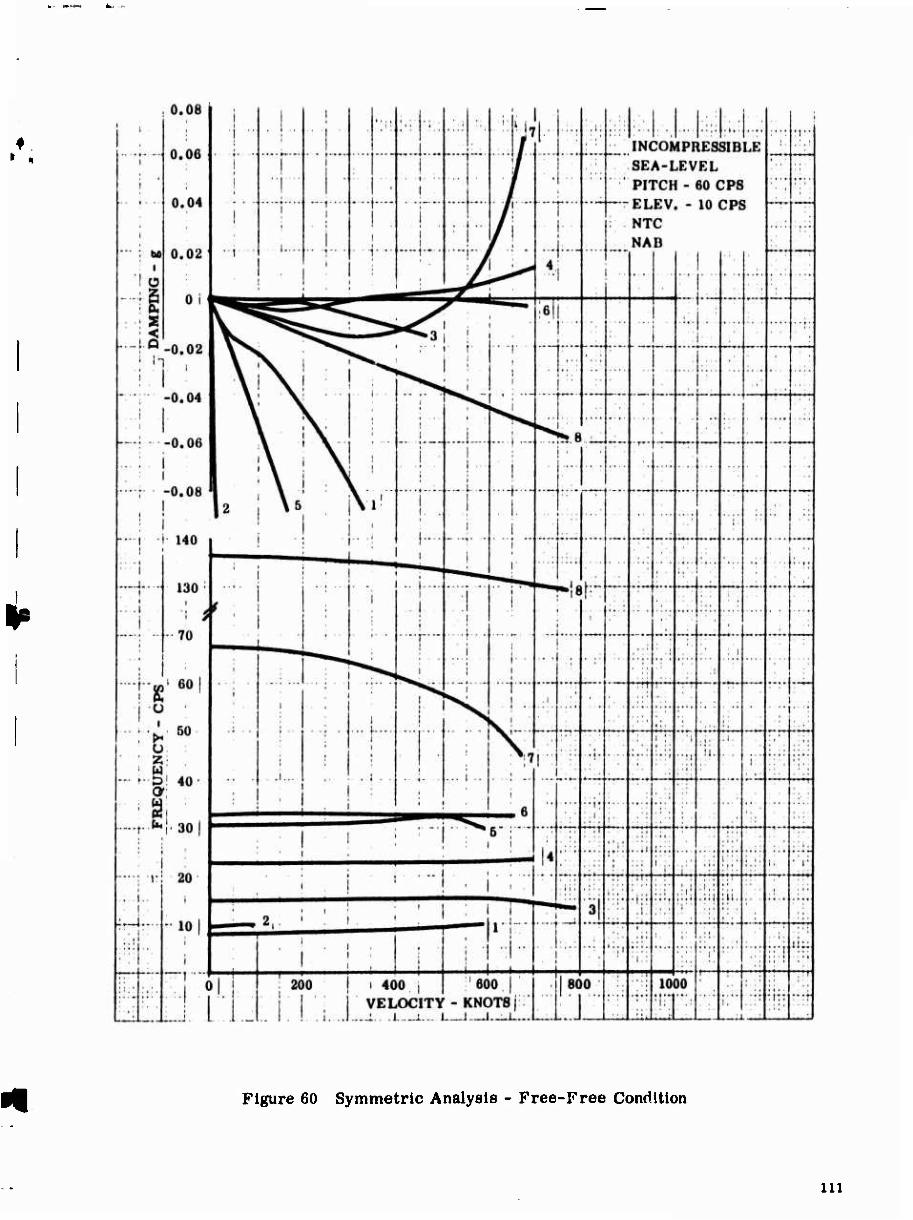
Figure 60 Symmetric Analysis - Free-Free Condition
in
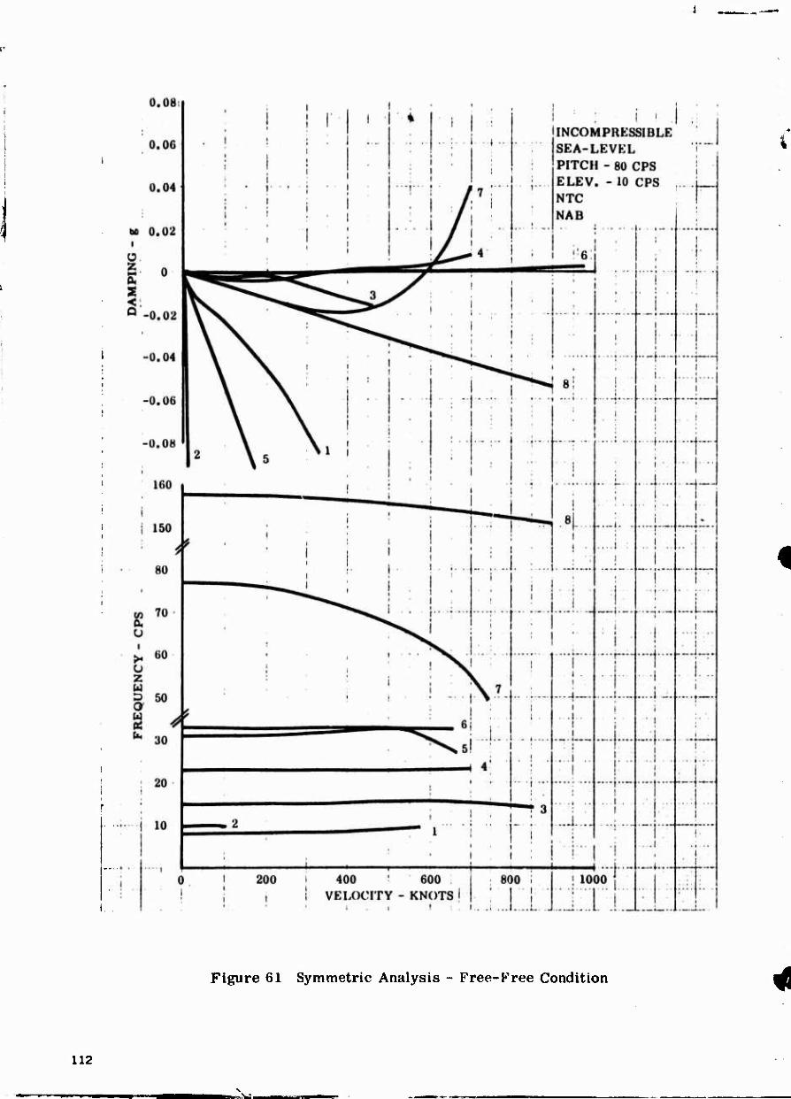
Figure 61 Symmetric Analysis - Free-Free Condition
112
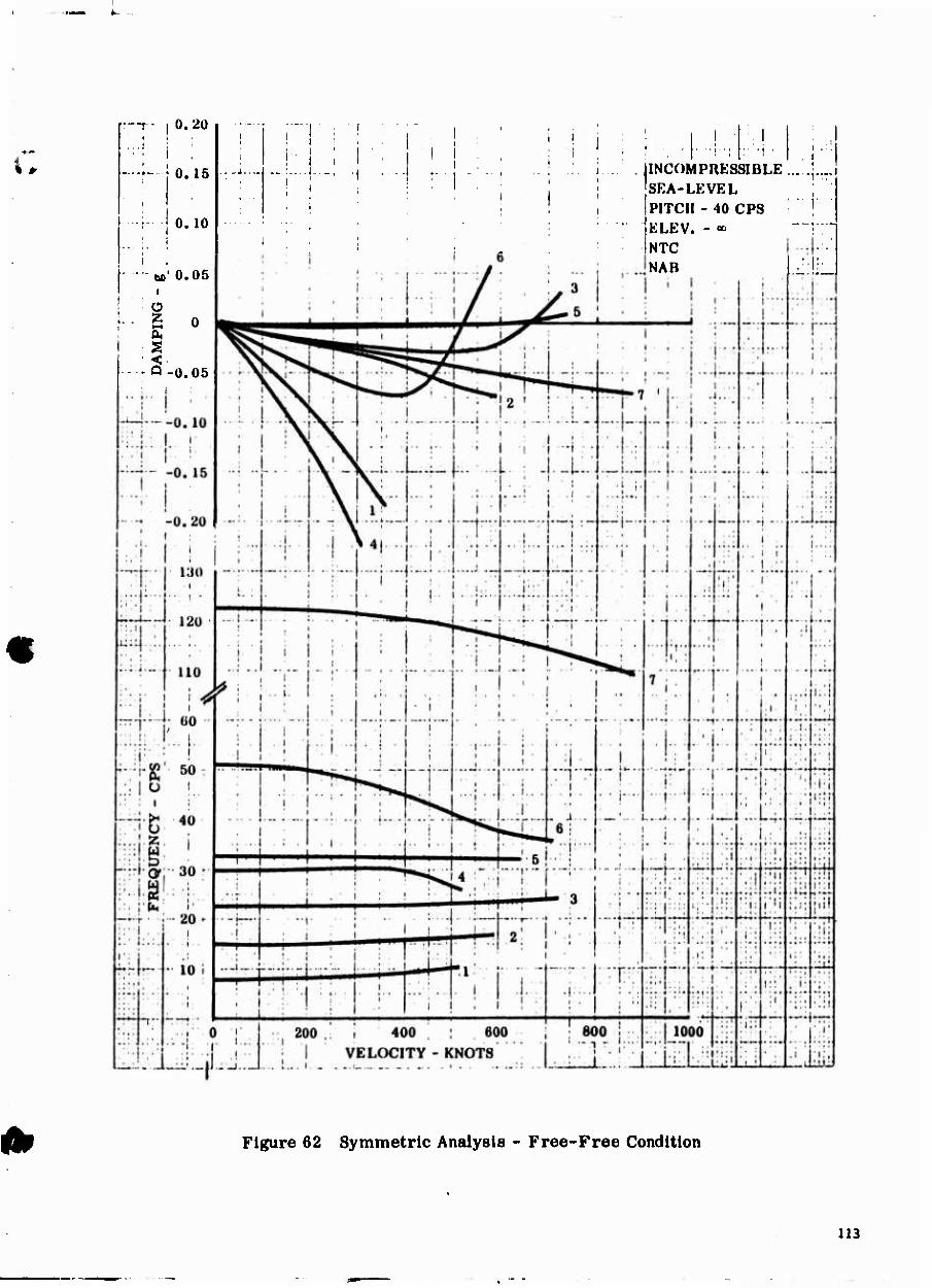
.—p.. ( 1
0.20
1 0.15
( 0.10
1 "*" bo ' 0.05
DA
MPI
NG -
0
-0.05
I , • •■,•■; :• -f , |-
JINCOMPRESSIBLE ... .|.„j SEA-LEVEL PITCH - 40 CPS ' ELEV. - « ~: NTC NAB
Figure 62 Symmetric Analysis - Free-Free Condition
113
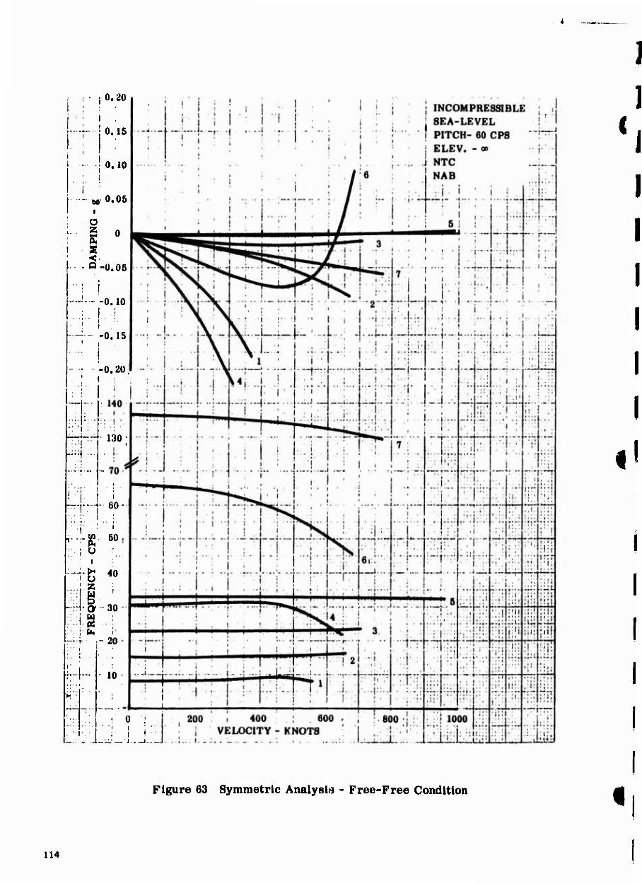
,♦.. .►•- . - 4
0.20
0.15
; INCOMPRESSIBLE ;
0.10
b0 w ■ uu
i
Ü
0 & s < Q -0. 05
j
! -0. 10
i i -0. 15
i •o. 20
~t--
:;q.. H- 130
--I.J- .'o.
1- -s I
50
• i w
-rg 40 l z
B •- •& 30 .:i.a ' ;'(* I ■ ... 20
•f" 10
I '. o ■; I ■ i -: .i-.n'_ i—i
c
Figure 63 Symmetric Analysiu - Free-Free Condition
114
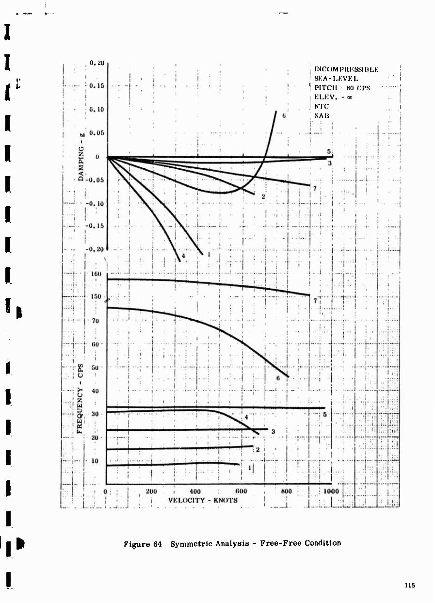
0.^0
i; INCOMIMIKSSIHLK SKA-LKVEL
1 PITCH - 80 CPS KLKV. - öD
NTC NAH
Figure 64 Symmetric Analysis - Free-Free Condition
115
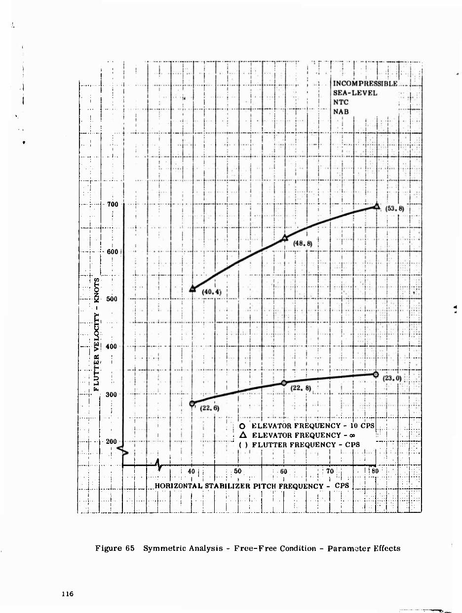
1 1
1
. .. 1 . .
1 .......
1 ■
i
1
-700 i
i
1
1 i
-600
-v 500
-Tg! 400
! -3 --.,, 300
200
-4-
..l
...j_...
i.
•H—h 40 j i
I i
O ELEVATOR FREQUENCY - 10 CPS i A ELEVATOR FREQUENCY - o>
( ) FLUTTER FREQUENCY - CPS
i 50 ■« i
60 ; 70
HORIZONTAL STABILIZER PITCH FREQUENCY - CPS
i
80 -.1^
Figure 65 Symmetric Analysis - Free-Free Condition - Parameter Effects
116
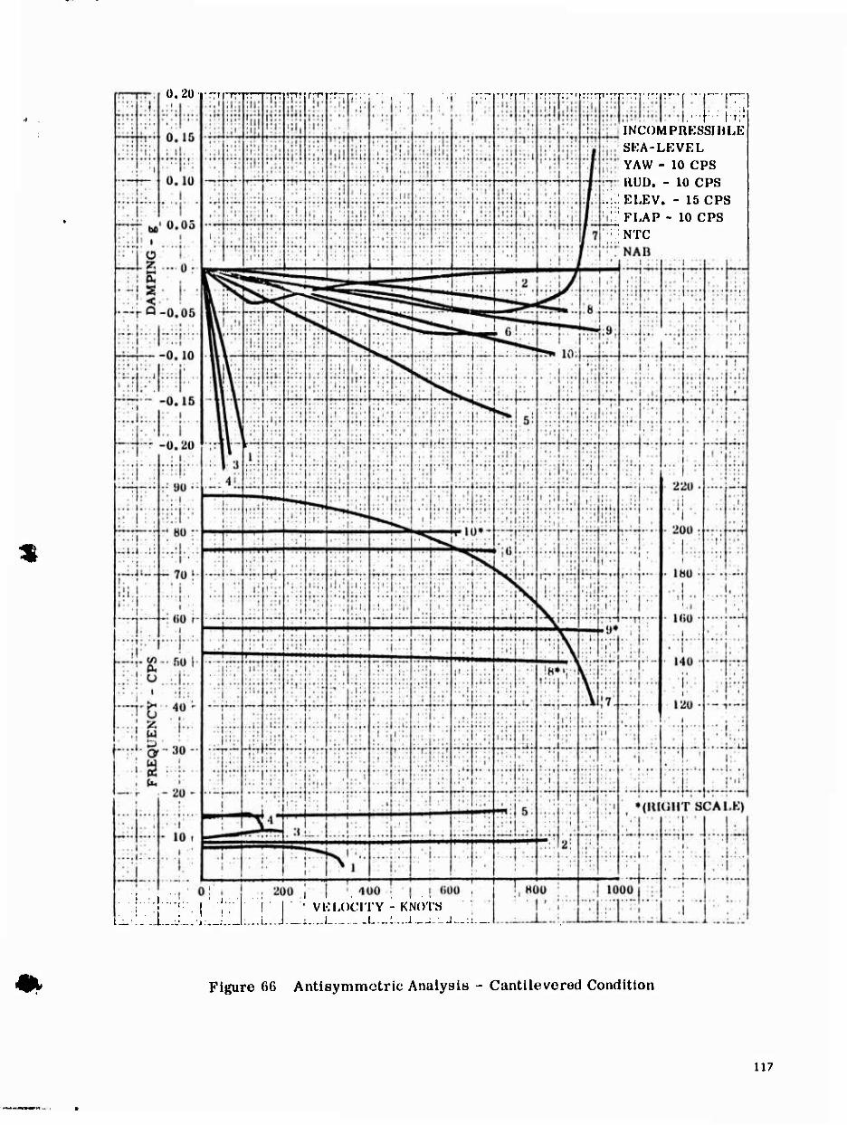
Ü.2Ü
INCOMPRESSIBLE SEA-LEVEL YAW - 10 CPS RUD. - 10 CPS
!^;ELEV. - 15 CPS FLAP - 10 CPS
^NTC
. • 1 ! ■ i I ' VELOCITY - KNOTS
„-L-J:—i-...L.. L._i_.i_J— -]...::._.
Figure 66 Antisymmetric Analysis - Cantilevered Condition
117
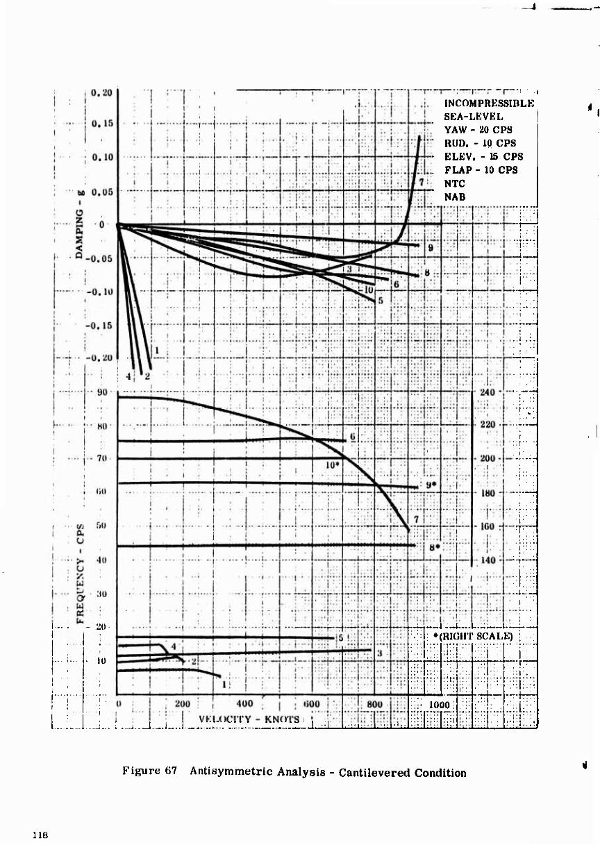
INCOMPRESSIBLE SEA-LEVEL YAW - 20 CPS RUD. - 10 CPS ELEV. - 15 CPS FLAP - 10 CPS NTC NAB
t . i
1 ■ 1
• 10
f
'■■•■;■■ ■ 1 ,
. , VKLOCITY - KNOTS | ; i ...J L_J 1—^ i—..- .— -j ._i -' "i i-l-l:;:'!.''
r
.a. i
(RIGHT SCALE) i
I
:;t; :
lv. 1000 M.
Figure 67 Antisymmetric Analysis - Cantilevered Condition
118
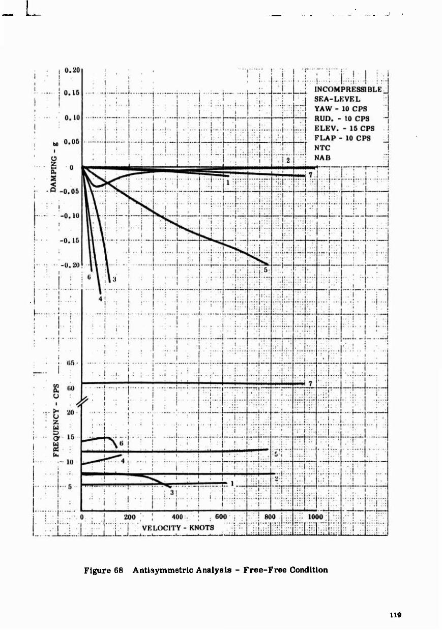
k. -.
Figure 68 Antlaymmetric Analysis - Free-Free Condition
119
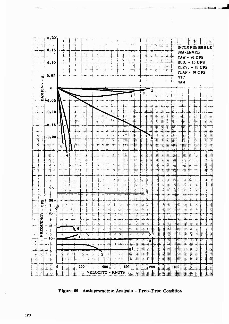
***&-
1—r- 1 * ■
.1.' 1 1
1 1
, 0,"20|
0.15
rO.lO
1
1
1
. ( . . .
"T"'
i i^ 1 ■ i •
f" i'" j" T" i .
t i [■ ■ , i ; I I
I " ' I ■! . . I t
i ■ ; i i
.: ■I. ;.i.
1
i 1
"I ■■'.;'. 1 ■ ' '
...... j.«. 1
; . :. .1
j....
h*~
1 1
j ( ■
i ■ ■*—
-■T-.y ■ ..'. ...; j: .:
: .:. ■ ; • 1
1
i INCOMPRESSIBLE SEA-LEVEL |
~"|H YAW - 20 CPS j '- RUD. - 10 CPS i ELEV. - 15 CPS
1
«■0,05 1
J u £ oi
0« i i 2'
1 • ' 1
...•■-. t .... ! I I l. ! . .. .-I . » i
i
t
\ , r.—i : FLAP- 10 CPS \
"~r NTC i NAH
J>^ ' • ! ZlZp*rfT*ti, ..J
•: ■! • .........
' i:;.
\:..u:.:.
1 :':"
t
• 0 1-0.05 I » 1 ' i
• ;■ i L-j. '-o.io l '• i I ■ ■'. ■ i
LL .In 1R
\\ LN. ^N
• j. _ ■ • i
"■*-'
i
1 ......i^ .
1 i :
.1.'..
•v|
r .
;,;:i:;;: •Hi
i. :;•
•H: i. ■
L... in: I ■
. I
i ■ i .. •■ ;;•■
.-■•i-
:rr ir- ■HH ■ *•*•
iiji •Hi ;::-
l';':i :.' ■ ■ < j . ■ - ■j
1 ' ■ '
j. I". -0.20 V1 ■'. "i. '■
l ^. ■ i
i t
N ;;:,: «
:-r:; r\\ '•-r iriri '•ri-
r.. IHH
; 1 ■
:H:i..iJ ... i
\\ . ■ i;: i .;
;';; i.:'
..:' 1:' ■. ....1....
I,;.!
....:
i,..
•:::
•:." U.'*^, rr.'. HH Hi- '■:;:
1 ' . . '
..H1" H ;.H
*~' '!TTn i .... ... i
i *
1. •. i;:,
..... .... ■::; •_
:
MlU ,:.■ •;
i i
■;; r ; *
i
r ■
... , ■■ 1 '"■ !r'-
■. ■!.; :
:;; ■ i:::: '••':': '•-.'■■ HH rv:
;;;i
''! i .iHri:
!
■■:■■ •;•
,. ■ .
—* i, !:';■ • i
1 ','.'.'. i ■! * i , : • i
1 : '
,... ."M ■.:
| :;f: Hi: TV- liiliii üiii^ .' 1"
;H; iH:|
* 1
'ii: : !|
i . "
•: 95- ■
i . ■ i .
-4- ... i.
. ;
>
....p..
;;:i : ■
■ 1
i,
' I..1-' ■■ i;:.:
:;... H;: :.-Hi rfr: ;!■;
; i.' H'
H ;i:.:i
■.. {■.:■■
■ 1 '■
i ' j' i -V,r, ; .
■ .; . ■
7;; :H: :;:: .... ::i:
HH .:;:i ; : ..; :. ■ ■
i i
• as ••
H|-uJ
T-i:b ;::.!:':: ;- '■ "'.'.'.' '::\ \ ■ ! 'S HH :iH *TT*
■
'.. "
■
... i!.J
•-•I
" ■ ■■[;•■'.'■
i. ■ 'i
W- •";'" ;:fT j.:;;
[; ■
rrr'H iiiiHH
;i!i
HH i::: '.'■',
rrir] ■•::
... i ,;
■•;
.... ..... :
••■:) •:•
.' 1 -••r— :■ ;|- ■
•; ': ■:
•~: "':' l*i*;
'■:- •rrr
. . , ...
«-•• - ■'.':' Hi; ■■ ,■ ;;
*-H ; ::i
Hr: :':•; •'•••
. HHi
-"^ ^^•h;'' ■ i^ji^ . * ', i ;'.:'; iHilii-; .... :iH: • ■* .■ Hi- ■':;
■ i;
iiii, ' 1
:;: ••• .., \^", :■{■.:' •!. ' ::;:; ■ ' ■ t i ! . i 5 III, ii-'
...i .
••: : •; ■1 .
rr? 5 -
'i
.; ; .1 : : :l ! 1 .:|.:. « , * I.. >. r j
• tit
; 1;. I ■ ■ . t
;.3
:; J 'T; t • * '
. t * • •
:iH
HH •::; I: i: • '"TV
..i. ■ ' ■ * 1 .HI -HJ
, ! ': I "^ ̂ v :.] . «1
! ' *' r :
■ i
... | .; i1 . i
■ i ;•
i. •
i 2 •■. j: ■ , *,■, :| *:■::
— m* mi it;; :;i'
:;!:
i!i;
H!;
;l::
iTi;,
i'i • *♦♦
i:;;
:i'\ 'rr ■HIT : t:n
':'...\r.. ( )'■■■■■ j 2nn !" ! : i AAA :! '■.'.'. . AAA 'I !;':• •.«-• M
■ ann . • •••« <
Hi"
Hi! 1AAA i '•'.' 1!!. 1
•Hi.- i
,:.i.. .I "- l i
VE LOCIT Y-KN OT S ; •■•■ ITT!
»t!. oiiiJ il Hi!
* <»■ Ml iiii iiii ULI " TTT *rn >*^ • »J
• • ■ 11 •4 -4 »4
Figure 69 Antisymmetric Analysis - Free-Free Condition
120