Working Paper No. 344

Preferences, Confusion and Competition

Andreas Hefti, Shuo Liu and Armin Schmutzler

April 2020

University of Zurich

Department of Economics

Working Paper Series

ISSN 1664-7041 (print) ISSN 1664-705X (online)

Preferences, Confusion and Competition

Andreas Hefti, Shuo Liu and Armin Schmutzler∗

April 30, 2020

Abstract

Do firms seek to make the market transparent, or do they confuse the consumers

in their product perceptions? We show that the answer to this question depends

decisively on preference heterogeneity. Contrary to the well-studied case of homo-

geneous goods, confusion is not necessarily an equilibrium in markets with differen-

tiated goods. In particular, if the taste distribution is polarized, so that indifferent

consumers are relatively rare, firms strive to fully educate consumers. By contrast,

if the taste distribution features a concentration of indecisive consumers, confusion

becomes part of the equilibrium strategies. The adverse welfare consequences of

confusion can be more severe than with homogeneous goods, as consumers may not

only pay higher prices, but also choose a dominated option, or inefficiently refrain

from buying. Qualitatively similar insights obtain for political contests, in which

candidates compete for voters with heterogeneous preferences.

Keywords: obfuscation, consumer confusion, differentiated products, price

competition, polarized/indecisive preferences, political competition.

JEL Classification: D43, L13, M30.∗Hefti: Department of Economics, University of Zurich and School of Management and Law, Zurich

University of Applied Science, heft@zhaw.ch. Liu: Guanghua School of Management, Peking Uni-

versity, shuo.liu@gsm.pku.edu.cn. Schmutzler: Department of Economics, University of Zurich and

CEPR, armin.schmutzler@econ.uzh.ch. We are grateful to Kfir Eliaz, Nils-Henrik von der Fehr, Paul

Heidhues, Justin Johnson, Heiko Karle, Kai Konrad, Changzhou Ma, Nick Netzer, Alexander Rasch,

Markus Reisinger, Mike Riordan, David Salant, Regina Seibel, Rani Spiegler, Jidong Zhou, and seminar

participants at Beijing (CUFE, UIEB), Dusseldorf, Frankfurt, MPI Munich, Nice, Shanghai (SUFE),

Tel Aviv, Zurich, EEA/ESEM (Cologne 2018), EARIE 2018 (Athens), EBE Summer Meeting 2018

(Herrsching), CRESSE 2018 (Heraklion), IO Workshop (St. Gallen), MaCCI 2019, Nanjing Microe-

conomics Workshop 2019, Workshop on Behavioral Economics and Mechanism Design (Glasgow) and

ESSET 2019 (Gerzensee), for many great discussions. Shuo Liu acknowledges the financial support by

the Forschungskredit of the University of Zurich (grant no. FK-17-018).

1

1 Introduction

When purchasing goods such as smartphones, motor vehicles or insurance, consumers

often make mistakes. To a certain extent, such mistakes reflect consumer confusion.

This has been documented across various sectors, including retailing, financial services,

utilities, telecommunication, the hospitality industry or health insurance (Eppler and

Mengis, 2004; Walsh et al., 2007; Loewenstein et al., 2013; Kasabov, 2015).1 Based

on several decades of evidence, there is a broad consensus in marketing science that

“consumers mix up, misidentify, or make wrong (i.e. illfounded) inferences about products

and/or erroneous product selections” (Mitchell and Kearney, 2002, p. 357).

Firms can influence the degree of confusion through their own activities. On the one

hand, firms can engage in measures to educate consumers: They can describe products

transparently to facilitate comparison, or they can inform consumers about their true

needs (e.g., by providing free trials). On the other hand, firms have means to confuse

consumers. For instance, insurance companies may issue contracts with complicated

premium-deductible schemes that impede comparisons with those of other firms. When

advertising differentiated products, firms may emphasize irrelevant product details rather

than those characteristics that really matter to consumers. Manufacturers of sophisti-

cated products, such as smartphones, digital cameras, or laundry machines, may add

attributes with unclear value to their products.

These issues are not specific to consumption choices. Like firms facing consumers,

political candidates facing voters can reduce confusion by stating their policies clearly,

or they can “becloud their policies in a fog of ambiguity” (Downs, 1957). The literature

suggests that “complexity, obfuscation, vagueness, and uncertainty are permanent fea-

tures of American electoral politics” (Gill, 2005, p. 372) and that candidates deliberately

obscure their positions (Downs, 1957; Franklin, 1991; Tomz and Van Houweling, 2009;

Rovny, 2012; Jacobson and Carson, 2015).

Do information providers, such as firms or political parties, seek to educate or confuse

their audiences? The special case of homogeneous choice options may suggest that the

answer is clear-cut. For example, oligopolistic producers of homogeneous goods suffer

from the temptation to undercut each others’ prices, resulting in a zero-profit equilib-

rium under well-known conditions.2 The literature on behavioral industrial organization

has shown that obfuscation techniques often allow firms to escape the “Bertrand trap”:

1See “Why the confusion of the cell phone market has caused millions to switch,” Forbes, May 2017,

for a recent report about consumer confusion in the cell phone industry.2Such an equilibrium arises, e.g., if the following conditions hold simultaneously: static interaction,

identical and constant marginal costs, no capacity constraints, complete information (Tirole, 1988).

2

Suppliers of homogeneous goods can secure positive profits in environments where the

same would be impossible if consumers were not confused.3 In this paper, we show that

firms need not benefit from, and may even be averse to consumer confusion in the case

of heterogeneous choice options. This may seem surprising, as the scope for confusion

with heterogeneous products is larger. For example, there can be many ways to present

the differences between products, and the dimensions that firms emphasize are likely to

influence the perceived valuations. Nevertheless, the incentives to confuse consumers are

less clear-cut, because firms usually obtain positive profits in differentiated goods mar-

kets even without obfuscation. Accordingly, by blurring the perception of consumers,

obfuscation may reduce rather than increase profits.

We introduce a general framework to uncover under which conditions strategic con-

testants (firms, political candidates, etc.), who compete for heterogeneous agents (con-

sumers, voters, etc.), communicate their choice options clearly or ambiguously, respec-

tively. The agents’ true preferences are characterized by a distribution of match values

for two contestants, who can influence their payoffs by choosing their communication

strategies and efforts.

The chosen communication strategies jointly determine the agents’ perception of prod-

uct valuations, potentially introducing errors to their comparisons of choice options.

Agent confusion arises if the perceived and true valuations disagree. We begin by assum-

ing that communication strategies influence the comparison of alternatives by inducing

stochastic perturbations, which do not affect the average valuation differences. Agent

confusion then results in unsystematic decision mistakes, meaning that the agents cannot

be systematically fooled.4 These perception errors can have different origins, such as

product complexity, attribute uncertainty or limited comparability because of framing

effects; see Section 4.1 for an intuitive discussion and Appendix S.1 for a formalization.

Contrary to communication strategies, the chosen efforts have unambiguous effects on

3For instance, firms can benefit from hidden fees (Gabaix and Laibson, 2006; Ellison and Ellison,

2009; Heidhues et al., 2016), spurious differentiation resulting from the credulity of consumers (Spiegler,

2006), product complexity (Gabaix and Laibson, 2004) or combative marketing (Eliaz and Spiegler,

2011a,b), from coarse thinking (Mullainathan et al., 2008), incomparable price formats (Carlin, 2009;

Piccione and Spiegler, 2012; Chioveanu and Zhou, 2013; Spiegler, 2014), from increasing consumer search

costs (Ellison and Wolitzky, 2012), or from consumers lacking (intertemporal) self-control (Heidhues and

Koszegi, 2017); see also Grubb (2015).4The unbiasedness assumption can be seen to play a similar disciplining role in our analysis as the

“conformity with the prior” assumption in Bayesian models of persuasion (Kamenica and Gentzkow,

2011), costly information acquisition (Caplin and Dean, 2015), or information design (Armstrong and

Zhou, 2019).

3

how the agents evaluate the contestants. Examples of such efforts are price reductions (a

lower price unambiguously increases the relative attractiveness for all consumers) or cer-

tain advertising measures (a more prominent option unambiguously captures relatively

more attention). The decisive feature of our analysis is that the interaction between the

communication strategies and the dispersion of true preferences determines the distribu-

tion of perceived valuations, and thereby the intensity of competition.

We formalize the above notions in a two-stage, non-cooperative, complete information

game, where the contestants first simultaneously choose their communication strategies

and then their efforts. Finally, each agent selects the contestant (buys a product, casts a

vote) which she perceives as offering the higher value to her.

Main Result Our main finding is that agent preferences play a decisive role for whether

confusion or education is supported as equilibrium outcome. While contestants always fa-

vor minimal competition, whether they can achieve this by confusing or educating agents

depends critically on the true dispersion of opinions in the agent population. We iden-

tify intuitive properties of the preference distribution that determine whether contestants

will engage in obfuscation or education. Specifically, we distinguish between indecisive

preferences, for which, loosely speaking, indifferent agents are relatively common, and

polarized preferences, for which strong opinions prevail. For instance, in a standard

textbook Hotelling model with symmetric firms, consumer preferences are indecisive (po-

larized) if the density of the consumer distribution has a maximum (minimum) at the

midpoint of the Hotelling interval.

Whether preferences are polarized or indecisive in a given setting is an empirical ques-

tion; both cases seem to be relevant. To illustrate the properties, consider the hospitality

industry. It is hard to imagine that most guests will be indifferent when faced with the

choice between a “family” hotel and a “business” hotel – instead, most consumers will

clearly prefer one alternative over the other, resulting in a polarized preference distri-

bution. By contrast, there will be many more undecided consumers if the comparison

is between two different business hotels, in line with indecisive preferences. In politics,

polarized preferences prevail when partisan tendencies are pronounced – whether this is

the case may vary across jurisdictions and time.

Education is the equilibrium outcome with polarized preferences if the range of deci-

sion mistakes is limited by the degree of true taste differentiation. This condition means

that, even for the largest possible mistake, the agent with the strongest preferences for

one contestant will not switch to the other contestant given identical efforts of the con-

testants. By contrast, there cannot be an equilibrium without agent confusion when

4

preferences are indecisive. Even stronger results emerge if the communication profiles

can be ordered in terms of the error dispersion they induce (e.g., by mean-preserving

spreads). With polarized preferences, education then is the only equilibrium outcome.

By contrast, with indecisive preferences the unique equilibrium features maximal con-

fusion, and the equilibrium communication profile leads to a more extreme dispersion

of perceived valuations compared to the true distribution. Finally, we consider the case

where obfuscation possibilities are “massive” relative to true preferences, meaning that

even the agents who are most loyal to a contestant could be confused enough to choose

the dominated option. Then, confusion may arise in equilibrium even with polarized

preferences.

Crucially, these results reflect the interplay between the shape of the true preference

distribution and the effects of communication. Competition forces contestants to fight

for the marginal agents, that is, for the agents who perceive the two options as equally

valuable. The larger the mass of such perceptually indifferent agents, the fiercer is compe-

tition, and the less profitable the market becomes. When true preferences are indecisive,

so that undecided “moderates” are common and “extremists” with strong opinions are

rare, confusion reduces the mass of perceptually indifferent agents, as it converts more

indecisive agents into extremists than vice versa. The opposite logic applies to the case of

polarization, where undecided agents are rare and those with strong opinions are common.

Then, education must decrease the mass of perceptually indifferent agents.

After presenting the general analysis, we derive some results that are more specific to

our two applications. For price competition, the welfare analysis differs substantially from

the homogeneous goods case studied by the literature. Absent a binding outside option,

the main effect of consumer confusion in a homogeneous good setting is redistribution

of rents from consumers to firms. By contrast, obfuscation implies that some consumers

choose dominated options in a differentiated goods setting, resulting in an inefficient mar-

ket outcome. We also show that policy measures directed at fostering competition, e.g.,

by means of product standardization, can backfire because they increase firms’ incentives

to confuse.

Further, we illustrate that the possibility of a binding outside option does not diminish

the firms’ incentives to obfuscate in the case of indecisive preferences: On the contrary,

firms may deliberately choose to engage in obfuscation even if this means that some con-

sumers (inefficiently) abstain from purchasing any product. This may help to understand

why confusion remains prevalent in many cases, despite the development of a large body

of “confusion reduction strategies” (Mitchell and Papavassiliou, 1999).5 Likewise, our

5See Chernev et al. (2015) for a survey of related issues. The marketing literature has occasionally

5

main results continue to apply if consumers differ in their degree of sophistication, or in

how prone to confusion they are (Walsh et al., 2007). All told, our analysis shows that

with differentiated goods, consumer confusion is less likely to arise in equilibrium than

with homogeneous goods, but if it occurs, its effects are more severe.6

When applied to political competition, our approach sheds new light on a long-

standing question in the literature. Various authors have asked why political candidates

or parties often choose ambiguous platforms rather than specifying their intended poli-

cies clearly (e.g., Shepsle, 1972; Aragones and Neeman, 2000; Callander and Wilson, 2008;

Kartik et al., 2017). Our analysis highlights the role of voter heterogeneity for this de-

cision. Candidates select ambiguous platforms if the share of indecisive voters is large.

In such a case, obfuscation distorts the preference distribution in such a way that strong

opinions become more common, and moderate views more rare. This is beneficial for

candidates, as it reduces the subsequent intensity of the campaign. By contrast, with

pre-existing polarization of the preference distribution, strategic candidates do not de-

sire ambiguous platforms, because voter confusion backfires by increasing the share of

indifferent voters.

The paper is organized as follows. Section 2 introduces the general framework. Section

3 presents the main results. Section 4 applies the general setting to product market

competition. Section 5 contains the application to political economy. Section 6 concludes.

All proofs and additional results are relegated to Appendices A and S.

2 The Model

A unit measure of agents needs to decide between the choice options offered by two

contestants i = 1, 2. Agent preferences are characterized by a distribution of match

values (vk1 , vk2) ∈ R2 for the contestants, where the match advantage of contestant i = 2

for agent k ∈ [0, 1] is given by vk∆ ≡ vk2 −vk1 . The match advantages vk∆ are dispersed over

the agent population according to an exogenously given distribution function G0, which

is commonly known by the contestants, and admits a zero-symmetric density function

conjectured that consumer confusion may serve to raise revenues (Mitchell and Papavassiliou, 1999;

Mitchell and Kearney, 2002; Haan and Berkey, 2002), but this issue has not been further explored yet

(Kasabov, 2015).6Our results also contrasts with Spiegler (2019), who asks whether agents with mis-specified causal

models can be systematically fooled as measured by biased expectations: We show that even if there

is no average perception bias, contestants may exploit the agents due to a competition softening effect

triggered by confusion.

6

g0 (i.e., g0(x) = g0(−x) ∀x ∈ R).7 Each contestant can influence the agents’ choices by

means of two different instruments.

On the one hand, each contestant can choose a communication strategy ai ∈ A from

some exogenously given set A. The respective communication profile (a1, a2) = a ∈ A ≡A2 influences the agents’ perception of the match advantages. For example, the com-

munication strategies could correspond to the ambiguity of the political platforms (see

Section 5), or to the marketing campaigns that influence which associations consumers

make when thinking about the product (Mullainathan et al., 2008). As we detail in

Section 4.1, they could also amount to “presentation formats” that jointly influence how

easy it is to compare the alternatives (Piccione and Spiegler, 2012; Chioveanu and Zhou,

2013; Spiegler, 2014), or they could reflect “product complexity” as determined by the

number of advertised product attributes (Mutzel and Kilian, 2016). For any communi-

cation profile a ∈ A, the perceived match advantage vk∆(a) of contestant i = 2 for agent

k is determined according to

vk∆(a) = vk∆ + εa. (1)

where εa is a (possibly degenerate) random variable with distribution function Γa, which

is independent of vk∆.8 Expression (1) yields an analytically convenient reduced form

to capture agent confusion, and one that is consistent with several key findings from

marketing, consumer research and psychology, which we elaborate in Section 4.1 and

Appendix S.1.9

On the other hand, each contestant can exert an “effort” si ∈ S ⊂ R to persuade

the agents to choose in his favor, given the dispersion of perceived match advantages

vk∆. For example, such efforts could correspond to the advertising intensities of political

candidates or firms, or they could represent (the negative of) product prices. Contrary to

communication strategies, efforts always have homogeneous effects on how agents evaluate

the contestants, where a higher si unambiguously increases every agent’s evaluation of

contestant i relative to his competitor. Specifically, agent k chooses contestant i = 1 if

and only if vk∆(a) ≤ s1 − s2, that is, the perceived match advantage of contestant 2 is

smaller than the effort advantage of contestant 1.

Let Ga denote the distribution function of the perceived match advantages vk∆ of

contestant i = 2. For any given communication-effort profile (a, (s1, s2)), the fraction of

7The formulation in terms of match advantages, rather than absolute values, highlights the compar-

ative nature of the agents’ thinking. Absent a binding outside option, this is without loss of generality

(see Section 4.4).8Our main insights do not hinge on the independence of εa and vk∆; see Appendix S.5 for an example.9Gabaix and Laibson (2004) and Kalaycı and Potters (2011) consider a similar additive structure of

the decision utility in the case of homogeneous preferences.

7

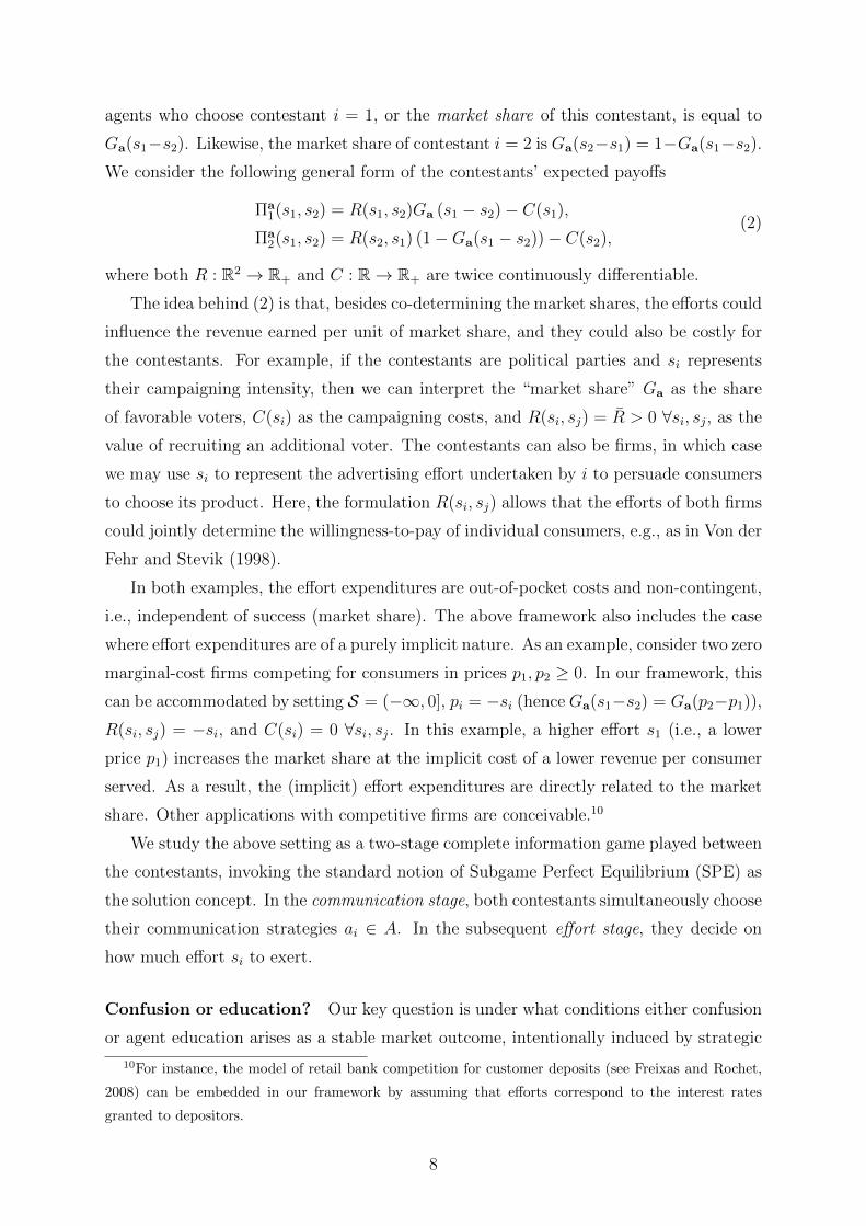
agents who choose contestant i = 1, or the market share of this contestant, is equal to

Ga(s1−s2). Likewise, the market share of contestant i = 2 is Ga(s2−s1) = 1−Ga(s1−s2).

We consider the following general form of the contestants’ expected payoffs

Πa1(s1, s2) = R(s1, s2)Ga (s1 − s2)− C(s1),

Πa2(s1, s2) = R(s2, s1) (1−Ga(s1 − s2))− C(s2),

(2)

where both R : R2 → R+ and C : R→ R+ are twice continuously differentiable.

The idea behind (2) is that, besides co-determining the market shares, the efforts could

influence the revenue earned per unit of market share, and they could also be costly for

the contestants. For example, if the contestants are political parties and si represents

their campaigning intensity, then we can interpret the “market share” Ga as the share

of favorable voters, C(si) as the campaigning costs, and R(si, sj) = R > 0 ∀si, sj, as the

value of recruiting an additional voter. The contestants can also be firms, in which case

we may use si to represent the advertising effort undertaken by i to persuade consumers

to choose its product. Here, the formulation R(si, sj) allows that the efforts of both firms

could jointly determine the willingness-to-pay of individual consumers, e.g., as in Von der

Fehr and Stevik (1998).

In both examples, the effort expenditures are out-of-pocket costs and non-contingent,

i.e., independent of success (market share). The above framework also includes the case

where effort expenditures are of a purely implicit nature. As an example, consider two zero

marginal-cost firms competing for consumers in prices p1, p2 ≥ 0. In our framework, this

can be accommodated by setting S = (−∞, 0], pi = −si (hence Ga(s1−s2) = Ga(p2−p1)),

R(si, sj) = −si, and C(si) = 0 ∀si, sj. In this example, a higher effort s1 (i.e., a lower

price p1) increases the market share at the implicit cost of a lower revenue per consumer

served. As a result, the (implicit) effort expenditures are directly related to the market

share. Other applications with competitive firms are conceivable.10

We study the above setting as a two-stage complete information game played between

the contestants, invoking the standard notion of Subgame Perfect Equilibrium (SPE) as

the solution concept. In the communication stage, both contestants simultaneously choose

their communication strategies ai ∈ A. In the subsequent effort stage, they decide on

how much effort si to exert.

Confusion or education? Our key question is under what conditions either confusion

or agent education arises as a stable market outcome, intentionally induced by strategic

10For instance, the model of retail bank competition for customer deposits (see Freixas and Rochet,

2008) can be embedded in our framework by assuming that efforts correspond to the interest rates

granted to depositors.

8

contestants. Specifically, can education be sustained as an equilibrium outcome if edu-

cating the agents is feasible for the contestants? If not, would the contestants want to

induce as much agent confusion as possible? The following definition clarifies our notions

of “confusion” and “education”.

Definition 1 We say that a communication profile a ∈ A induces agent confusion (is ob-

fuscating) if vk∆(a) and vk∆ are not equal in distribution, i.e., Ga 6= G0. A communication

profile a ∈ A induces agent education (is educating) if Ga = G0.

Throughout the main analysis, we suppose that the effects of communication on the

agents’ perception of the match advantages are unbiased, meaning that εa in (1) is zero-

symmetrically dispersed. In other words, we assume that for any given a ∈ A, either (i)

εa = O, where O is any random variable that is almost surely equal to zero, or (ii) the

distribution function of εa satisfies Γa(x) = 1 − Γa(−x) ∀x ∈ R. We take Γa to have a

density γa whenever εa 6= O.

Intuitively, the zero-symmetry of εa implies that while the contestants may be able

to increase or decrease the noise in the perception process, they cannot systematically

bias the perceived match advantage distribution.11 Such unbiasedness is consistent with

how the notion of confusion is often used, for instance, in the marketing literature; see

Section 4 and Appendix S.1. As an illustration, suppose that each contestant can choose

product “features” (attributes, advertising slogans, labels,...), where each feature has an

i.i.d. effect on the consumer evaluation of that product. Then, the number ai ∈ A ⊂ Nof features implemented corresponds to the communication strategy of contestant i, and

quantifies i’s contribution to agent confusion. The unbiasedness assumption means that

some consumers value the addition of such additional features, whereas others are put

off by the increase in complexity. Viewed through this lens, the core question of our

paper is whether rational contestants would ever seek to implement features with such

double-edged effects.

What matters for our analysis is that the contestants can possibly induce noise in the

comparisons made by the agents. While in this paper we emphasize various behavioral

explanations for confusion, we do not mean to exclude that similar perception errors

could also arise from a highly sophisticated decision process.12 As we show in Section

11This does not rule out that communication can bias the levels of the perceived match values (vk1 , vk2 ).

We consider such a possibility in Section 5.2. Moreover, unbiasedness does not require that v∆ and εa

are independent; see Appendix S.5 for an illustrative example.12As an example, it is a common result in models with noisy signals that Bayesian agents condition

their actions on the signals they observe. That is, while the agents behave deterministically according to

their posterior expectations, the expectations themselves are stochastic, as they depend on the particular

9

4.5, our results also apply with differentially sophisticated agents.

Together with the symmetry of G0, the unbiasedness of εa implies that the perceived

match advantage distribution, which is given by Ga(v) =∫G0(v−e)dΓa(e), with density

ga(v) =∫g0(v − e)dΓa(e), is itself zero-symmetric. These expressions reveal a simple

interaction between true preferences, captured by G0, and the perception errors induced

by communication profile a, which is decisive for whether confusion or education are

equilibrium phenomena, as we show in the next section.

3 Equilibrium Analysis

We derive the SPE of the game by backward induction. Section 3.1 characterizes the

symmetric second-stage effort equilibrium. Section 3.2 shows how preferences determine

whether confusion can arise in equilibrium. Sections 3.3 and Section 3.4 sharpen the

equilibrium predictions.

3.1 The Effort Stage

The payoff functions (2) together with the symmetry of G0 and Γa imply that the con-

testants play a symmetric game in the competition stage for any given a ∈ A. The

subsequent analysis concentrates on symmetric equilibria (s1 = s2 = s) in the effort

stage.13 For the equilibrium analysis, we require a technical assumption which, as we

show in Sections 4 and 5, holds in our major applications to price and political competi-

tion.

Assumption 1 The following conditions are satisfied:

(A1.1) Πai (si, sj) is strictly quasi-concave in si, ∀sj ∈ S, a ∈ A and i, j = 1, 2.

(A1.2) ∀a ∈ A ∃ s ∈ S such that z(s) = ga(0), where

ga(0) ≡∫g0(−e)dΓa(e) > 0, z(s) ≡

(C ′(s)

R(s, s)− R1(s, s)

2R(s, s)

),

and R` is the partial derivative of R with respect to its `-th argument.

(A1.3) z(s) is strictly increasing, and R1(s, s) +R2(s, s) < 2C ′(s) ∀s ∈ S.

signal that has realized. See Johnson and Myatt (2006) for an example, where noisy valuations arise as

posterior expectations induced by more or less noisy advertising.13A symmetric (stage) game with a differentiable structure, as the one studied here, always has a

symmetric equilibrium, while asymmetric equilibria exist only under special circumstances (Hefti, 2017).

10

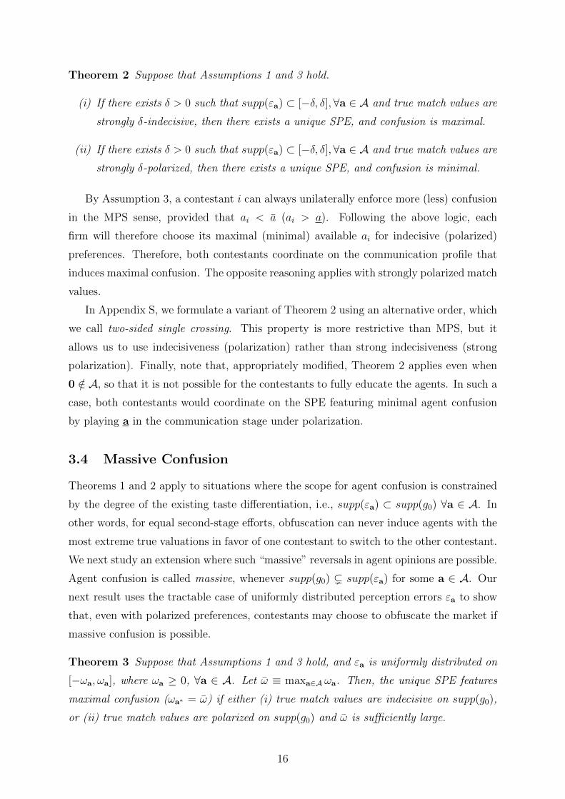
𝑠𝑠

𝑔𝑔𝒂𝒂(0) 𝑔𝑔𝒂𝒂𝒂(0)

𝑠𝑠𝒂𝒂∗

𝑧𝑧(𝑠𝑠)

Π

Π(𝑠𝑠)

Π 𝑔𝑔𝒂𝒂(0) Π 𝑔𝑔𝒂𝒂𝒂(0)

𝑠𝑠𝒂𝒂𝒂∗

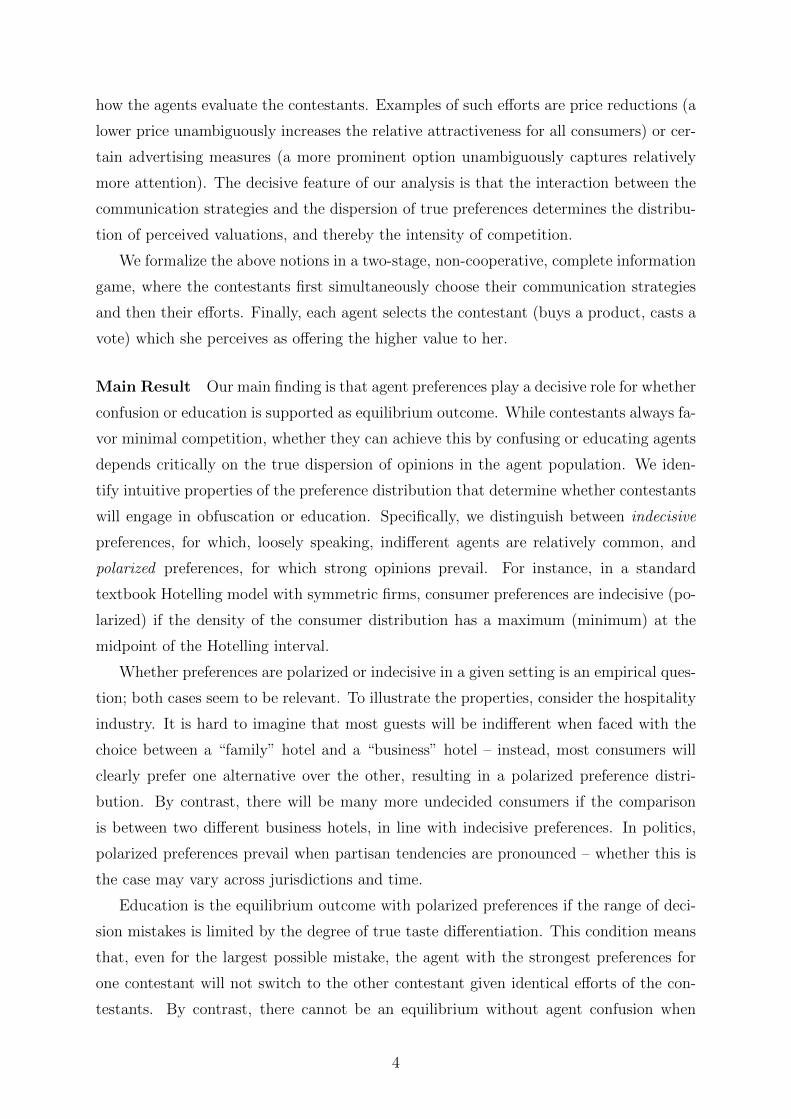
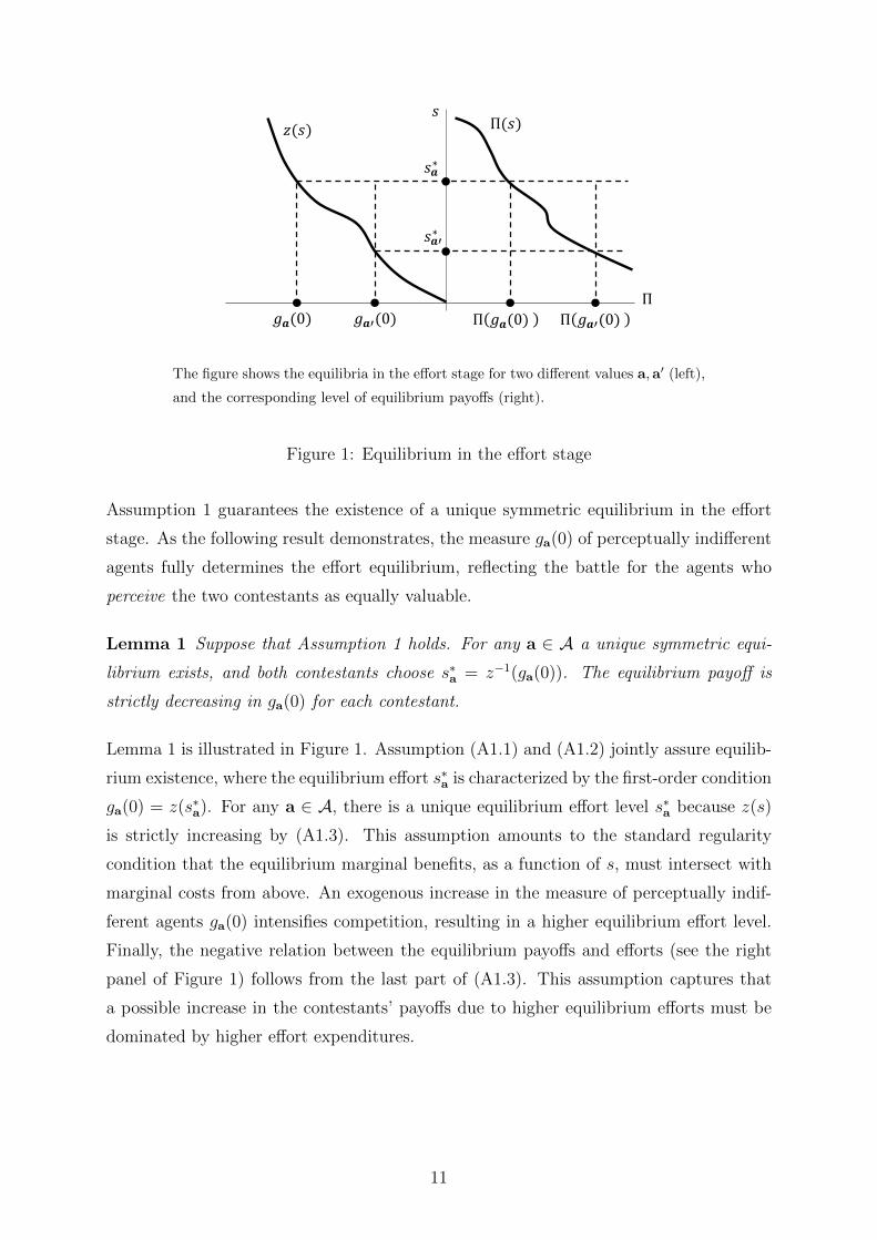
The figure shows the equilibria in the effort stage for two different values a,a′ (left),

and the corresponding level of equilibrium payoffs (right).

Figure 1: Equilibrium in the effort stage

Assumption 1 guarantees the existence of a unique symmetric equilibrium in the effort

stage. As the following result demonstrates, the measure ga(0) of perceptually indifferent

agents fully determines the effort equilibrium, reflecting the battle for the agents who

perceive the two contestants as equally valuable.

Lemma 1 Suppose that Assumption 1 holds. For any a ∈ A a unique symmetric equi-

librium exists, and both contestants choose s∗a = z−1(ga(0)). The equilibrium payoff is

strictly decreasing in ga(0) for each contestant.

Lemma 1 is illustrated in Figure 1. Assumption (A1.1) and (A1.2) jointly assure equilib-

rium existence, where the equilibrium effort s∗a is characterized by the first-order condition

ga(0) = z(s∗a). For any a ∈ A, there is a unique equilibrium effort level s∗a because z(s)

is strictly increasing by (A1.3). This assumption amounts to the standard regularity

condition that the equilibrium marginal benefits, as a function of s, must intersect with

marginal costs from above. An exogenous increase in the measure of perceptually indif-

ferent agents ga(0) intensifies competition, resulting in a higher equilibrium effort level.

Finally, the negative relation between the equilibrium payoffs and efforts (see the right

panel of Figure 1) follows from the last part of (A1.3). This assumption captures that

a possible increase in the contestants’ payoffs due to higher equilibrium efforts must be

dominated by higher effort expenditures.

11

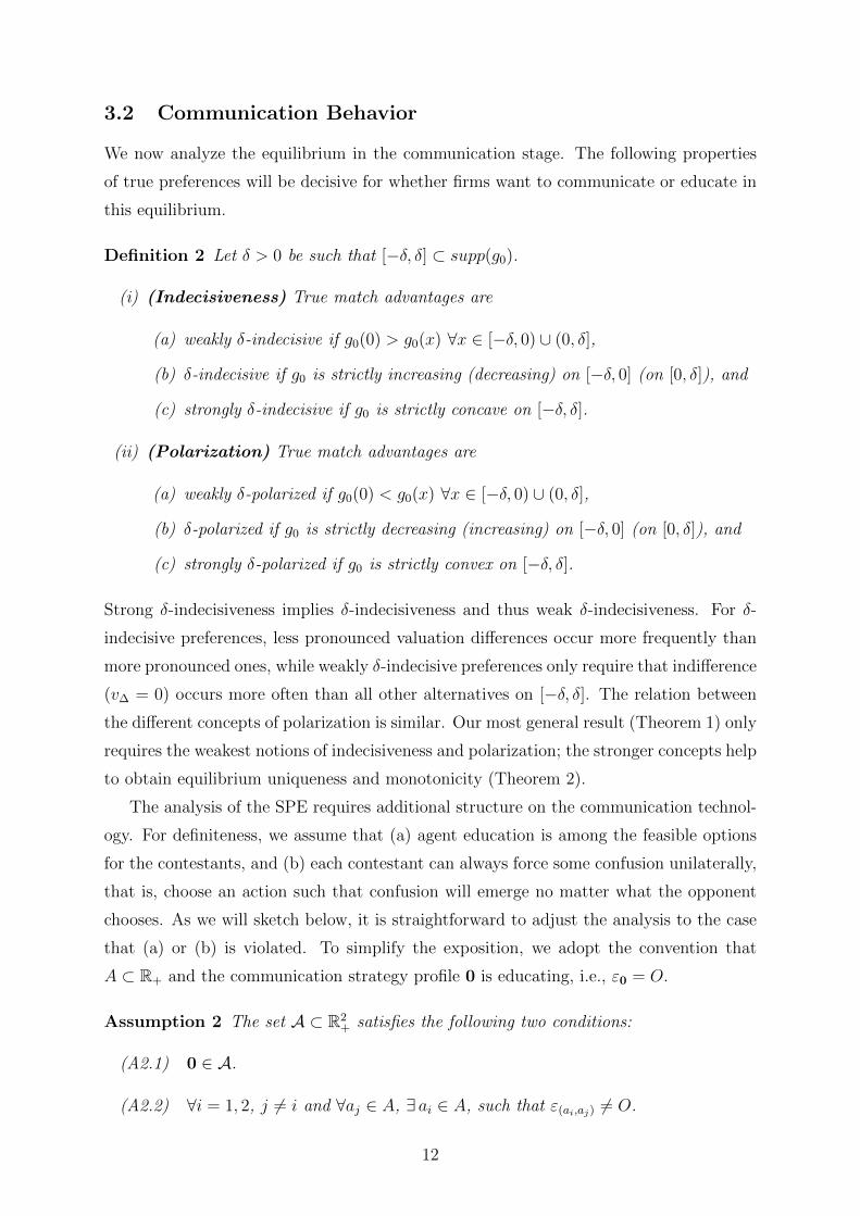
3.2 Communication Behavior

We now analyze the equilibrium in the communication stage. The following properties

of true preferences will be decisive for whether firms want to communicate or educate in

this equilibrium.

Definition 2 Let δ > 0 be such that [−δ, δ] ⊂ supp(g0).

(i) (Indecisiveness) True match advantages are

(a) weakly δ-indecisive if g0(0) > g0(x) ∀x ∈ [−δ, 0) ∪ (0, δ],

(b) δ-indecisive if g0 is strictly increasing (decreasing) on [−δ, 0] (on [0, δ]), and

(c) strongly δ-indecisive if g0 is strictly concave on [−δ, δ].

(ii) (Polarization) True match advantages are

(a) weakly δ-polarized if g0(0) < g0(x) ∀x ∈ [−δ, 0) ∪ (0, δ],

(b) δ-polarized if g0 is strictly decreasing (increasing) on [−δ, 0] (on [0, δ]), and

(c) strongly δ-polarized if g0 is strictly convex on [−δ, δ].

Strong δ-indecisiveness implies δ-indecisiveness and thus weak δ-indecisiveness. For δ-

indecisive preferences, less pronounced valuation differences occur more frequently than

more pronounced ones, while weakly δ-indecisive preferences only require that indifference

(v∆ = 0) occurs more often than all other alternatives on [−δ, δ]. The relation between

the different concepts of polarization is similar. Our most general result (Theorem 1) only

requires the weakest notions of indecisiveness and polarization; the stronger concepts help

to obtain equilibrium uniqueness and monotonicity (Theorem 2).

The analysis of the SPE requires additional structure on the communication technol-

ogy. For definiteness, we assume that (a) agent education is among the feasible options

for the contestants, and (b) each contestant can always force some confusion unilaterally,

that is, choose an action such that confusion will emerge no matter what the opponent

chooses. As we will sketch below, it is straightforward to adjust the analysis to the case

that (a) or (b) is violated. To simplify the exposition, we adopt the convention that

A ⊂ R+ and the communication strategy profile 0 is educating, i.e., ε0 = O.

Assumption 2 The set A ⊂ R2+ satisfies the following two conditions:

(A2.1) 0 ∈ A.

(A2.2) ∀i = 1, 2, j 6= i and ∀aj ∈ A, ∃ ai ∈ A, such that ε(ai,aj) 6= O.

12

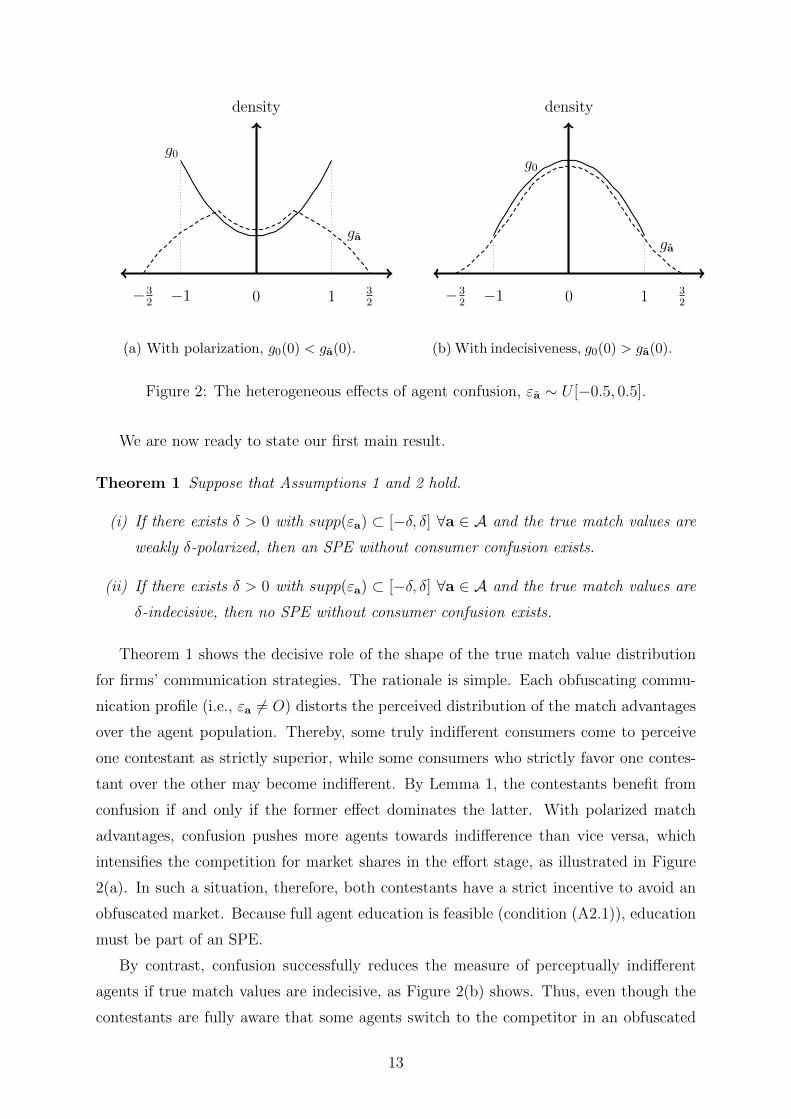
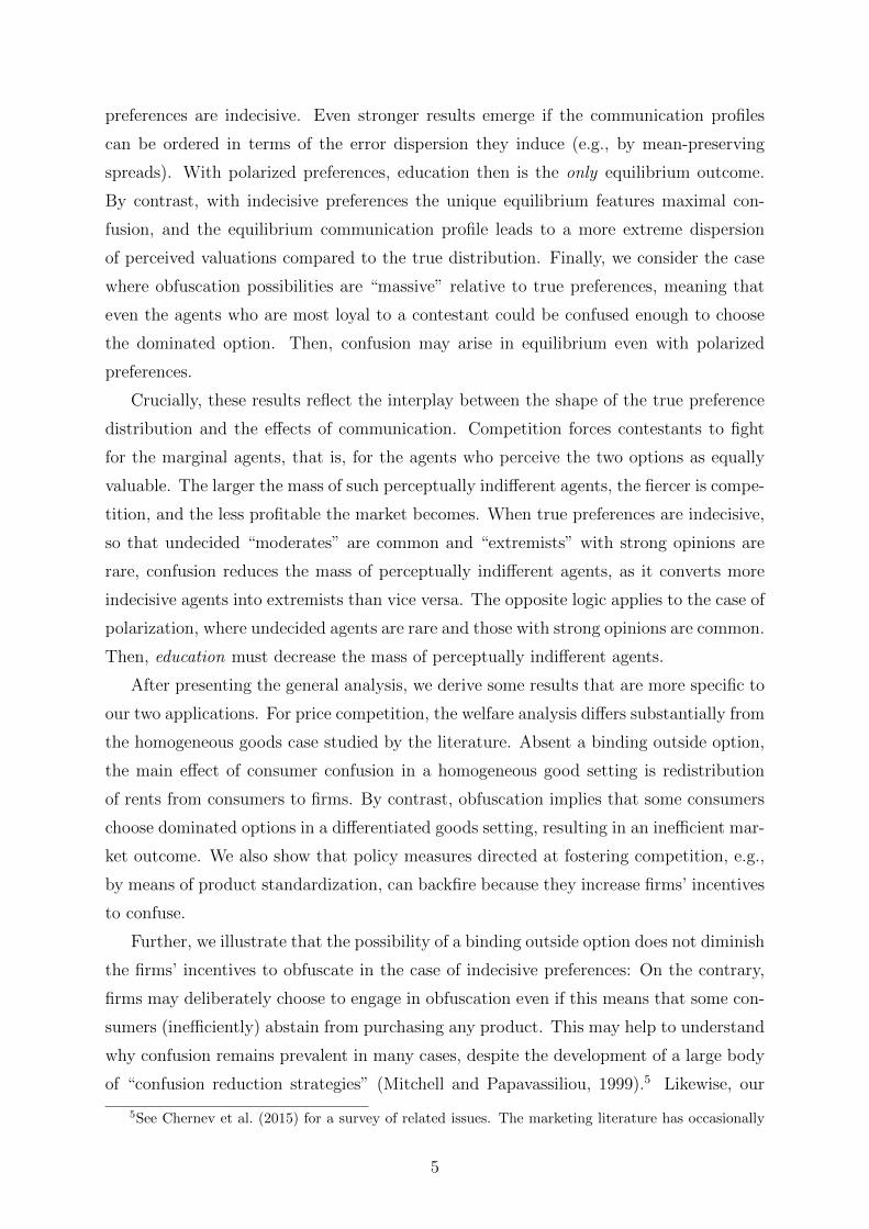
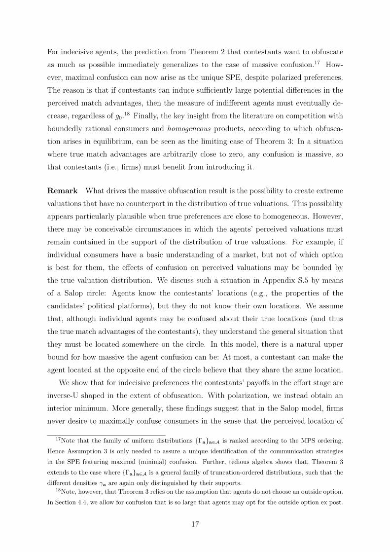
density

g0

ga

0−1 1−32

32

(a) With polarization, g0(0) < ga(0).

density

0−1 1−32

32

g0

ga

(b) With indecisiveness, g0(0) > ga(0).

Figure 2: The heterogeneous effects of agent confusion, εa ∼ U [−0.5, 0.5].

We are now ready to state our first main result.

Theorem 1 Suppose that Assumptions 1 and 2 hold.

(i) If there exists δ > 0 with supp(εa) ⊂ [−δ, δ] ∀a ∈ A and the true match values are

weakly δ-polarized, then an SPE without consumer confusion exists.

(ii) If there exists δ > 0 with supp(εa) ⊂ [−δ, δ] ∀a ∈ A and the true match values are

δ-indecisive, then no SPE without consumer confusion exists.

Theorem 1 shows the decisive role of the shape of the true match value distribution

for firms’ communication strategies. The rationale is simple. Each obfuscating commu-

nication profile (i.e., εa 6= O) distorts the perceived distribution of the match advantages

over the agent population. Thereby, some truly indifferent consumers come to perceive

one contestant as strictly superior, while some consumers who strictly favor one contes-

tant over the other may become indifferent. By Lemma 1, the contestants benefit from

confusion if and only if the former effect dominates the latter. With polarized match

advantages, confusion pushes more agents towards indifference than vice versa, which

intensifies the competition for market shares in the effort stage, as illustrated in Figure

2(a). In such a situation, therefore, both contestants have a strict incentive to avoid an

obfuscated market. Because full agent education is feasible (condition (A2.1)), education

must be part of an SPE.

By contrast, confusion successfully reduces the measure of perceptually indifferent

agents if true match values are indecisive, as Figure 2(b) shows. Thus, even though the

contestants are fully aware that some agents switch to the competitor in an obfuscated

13

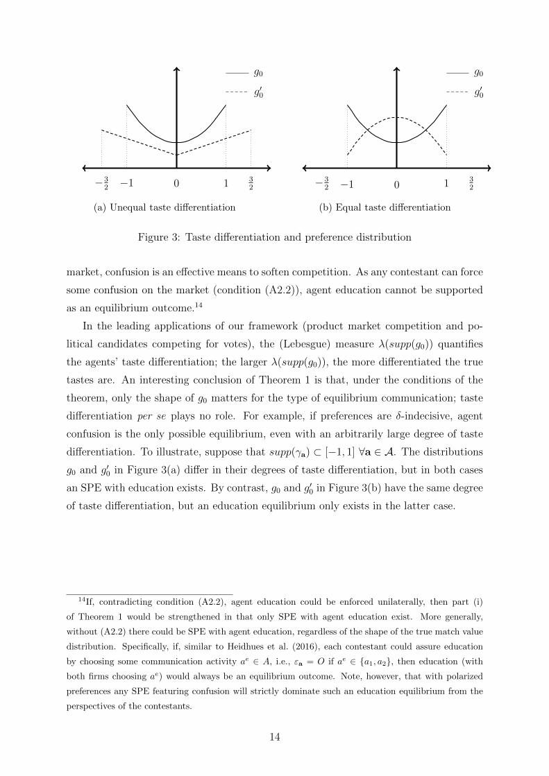
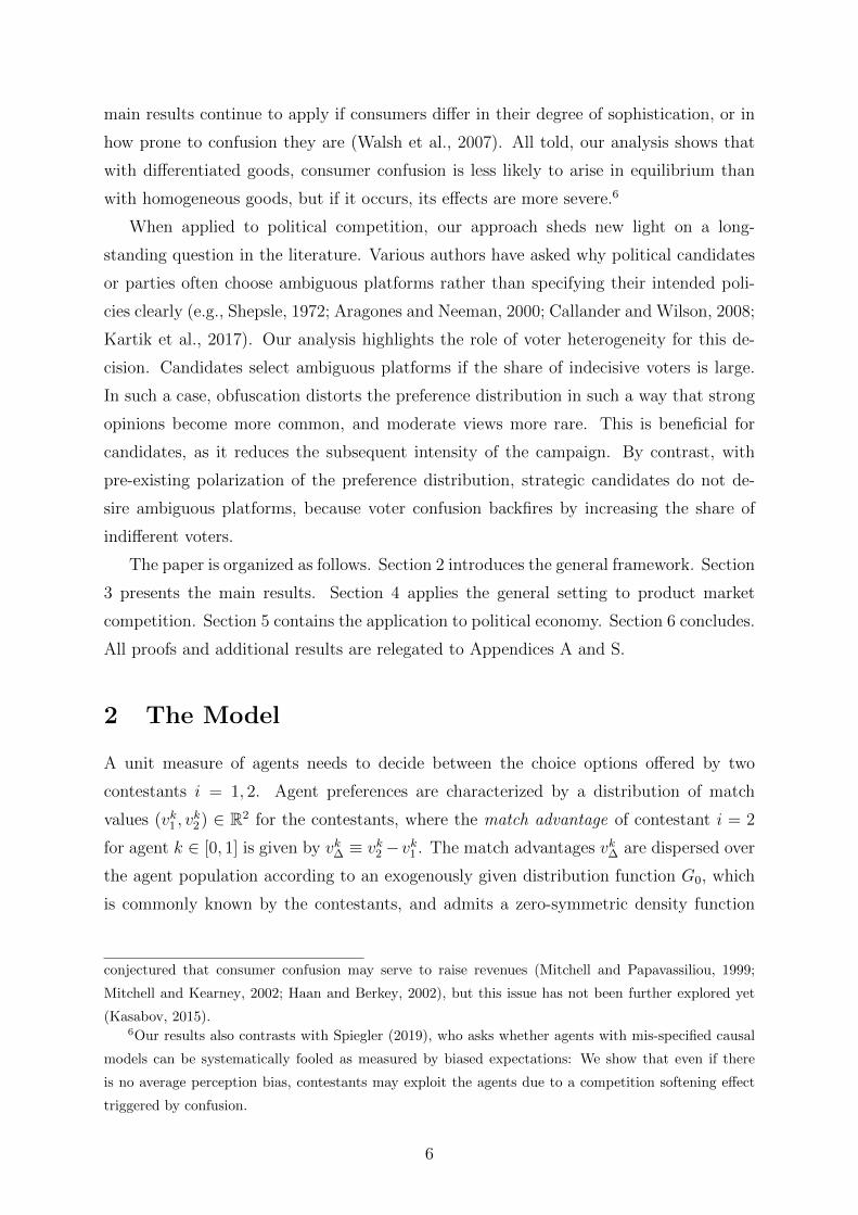
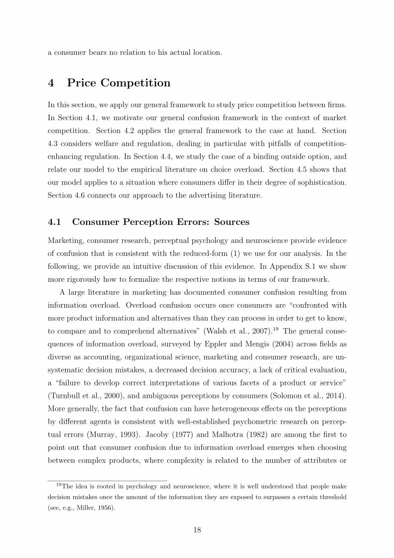
0−1 1−32

32

g0

g′0

(a) Unequal taste differentiation

0−1 1−32

32

g0

g′0

(b) Equal taste differentiation

Figure 3: Taste differentiation and preference distribution

market, confusion is an effective means to soften competition. As any contestant can force

some confusion on the market (condition (A2.2)), agent education cannot be supported

as an equilibrium outcome.14

In the leading applications of our framework (product market competition and po-

litical candidates competing for votes), the (Lebesgue) measure λ(supp(g0)) quantifies

the agents’ taste differentiation; the larger λ(supp(g0)), the more differentiated the true

tastes are. An interesting conclusion of Theorem 1 is that, under the conditions of the

theorem, only the shape of g0 matters for the type of equilibrium communication; taste

differentiation per se plays no role. For example, if preferences are δ-indecisive, agent

confusion is the only possible equilibrium, even with an arbitrarily large degree of taste

differentiation. To illustrate, suppose that supp(γa) ⊂ [−1, 1] ∀a ∈ A. The distributions

g0 and g′0 in Figure 3(a) differ in their degrees of taste differentiation, but in both cases

an SPE with education exists. By contrast, g0 and g′0 in Figure 3(b) have the same degree

of taste differentiation, but an education equilibrium only exists in the latter case.

14If, contradicting condition (A2.2), agent education could be enforced unilaterally, then part (i)

of Theorem 1 would be strengthened in that only SPE with agent education exist. More generally,

without (A2.2) there could be SPE with agent education, regardless of the shape of the true match value

distribution. Specifically, if, similar to Heidhues et al. (2016), each contestant could assure education

by choosing some communication activity ae ∈ A, i.e., εa = O if ae ∈ {a1, a2}, then education (with

both firms choosing ae) would always be an equilibrium outcome. Note, however, that with polarized

preferences any SPE featuring confusion will strictly dominate such an education equilibrium from the

perspectives of the contestants.

14

3.3 How Much Confusion?

Up to this point we have put no order structure on the various distribution functions

{Γa}a∈A. Given that consumer confusion is of an unbiased nature, a natural starting

point is to presume that the distribution functions {Γa}a∈A can be ordered using the

notion of a mean-preserving spread (MPS). Formally, for two random variables X and

Y , Y is an MPS of X if Y has the same distribution as X + η, where η 6= O and

E[η|X] = 0.15 Intuitively, Y is a noisy version of X. The above assumptions trivially

imply that any communication profile inducing confusion corresponds to an MPS of the

distribution corresponding to an educating profile. We now require more generally that

all noise distributions can be ordered via MPS.

Assumption 3 (MPS ordering) A ⊂ R+ is compact, and εa = O ⇔ a = 0. More-

over, ∀a, a′ ∈ A with a 6= a′ and a ≤ a′, Γa′ is an MPS of Γa.

Note that Assumption 3 implies Assumption 2 whenever 0 ∈ A and A contains more than

one element. Moreover, agent confusion is maximal (minimal) according to the MPS order

if both firms choose a ≡ maxA (a ≡ minA). In particular, the communication profile

(a, a) induces maximal agent confusion as measured by the variance of the perceived

match advantages.

Most examples we discuss in Appendix S.1 to support (1) feature the MPS ordering.

For instance, consider the above-mentioned example where communication strategies

correspond to the number of i.i.d features implemented by a contestant: The more such

features are implemented, the more noisy the perceived valuations become. Another class

of examples arises when the members of the family {Γa}a∈A are truncations of each other.

This order conveniently preserves essential features of the original distribution, such as

log-concavity of the density or the shape of γa. This essentially amounts to assuming that

greater confusion increases the scope for the possible perception errors, while leaving the

underlying stochastic principles behind the perception errors unaltered.16

Our second main result strengthens Theorem 1 by showing that under the MPS or-

dering a unique SPE exists, featuring either maximal or minimal confusion, depending

on the distribution of true preferences.

15Rothschild and Stiglitz (1970) show that if the involved distribution functions have a uniformly

bounded support, then the MPS ordering between distributions is equivalent to the order induced by

second-order stochastic dominance. Muller (1998) shows how to extend this equivalence to the case of

an unbounded support.16For any given a ∈ A, Γa is the truncation εa ≡ ε|ε∈[−ωa,ωa] of a random variable ε with zero-

symmetric density γ and supp γ = (−ω, ω), 0 ≤ ωa < ω. Then, Γa′ is an MPS of Γa iff ωa′ > ωa.

15

Theorem 2 Suppose that Assumptions 1 and 3 hold.

(i) If there exists δ > 0 such that supp(εa) ⊂ [−δ, δ],∀a ∈ A and true match values are

strongly δ-indecisive, then there exists a unique SPE, and confusion is maximal.

(ii) If there exists δ > 0 such that supp(εa) ⊂ [−δ, δ],∀a ∈ A and true match values are

strongly δ-polarized, then there exists a unique SPE, and confusion is minimal.

By Assumption 3, a contestant i can always unilaterally enforce more (less) confusion

in the MPS sense, provided that ai < a (ai > a). Following the above logic, each

firm will therefore choose its maximal (minimal) available ai for indecisive (polarized)

preferences. Therefore, both contestants coordinate on the communication profile that

induces maximal confusion. The opposite reasoning applies with strongly polarized match

values.

In Appendix S, we formulate a variant of Theorem 2 using an alternative order, which

we call two-sided single crossing. This property is more restrictive than MPS, but it

allows us to use indecisiveness (polarization) rather than strong indecisiveness (strong

polarization). Finally, note that, appropriately modified, Theorem 2 applies even when

0 /∈ A, so that it is not possible for the contestants to fully educate the agents. In such a

case, both contestants would coordinate on the SPE featuring minimal agent confusion

by playing a in the communication stage under polarization.

3.4 Massive Confusion

Theorems 1 and 2 apply to situations where the scope for agent confusion is constrained

by the degree of the existing taste differentiation, i.e., supp(εa) ⊂ supp(g0) ∀a ∈ A. In

other words, for equal second-stage efforts, obfuscation can never induce agents with the

most extreme true valuations in favor of one contestant to switch to the other contestant.

We next study an extension where such “massive” reversals in agent opinions are possible.

Agent confusion is called massive, whenever supp(g0) ( supp(εa) for some a ∈ A. Our

next result uses the tractable case of uniformly distributed perception errors εa to show

that, even with polarized preferences, contestants may choose to obfuscate the market if

massive confusion is possible.

Theorem 3 Suppose that Assumptions 1 and 3 hold, and εa is uniformly distributed on

[−ωa, ωa], where ωa ≥ 0, ∀a ∈ A. Let ω ≡ maxa∈A ωa. Then, the unique SPE features

maximal confusion (ωa∗ = ω) if either (i) true match values are indecisive on supp(g0),

or (ii) true match values are polarized on supp(g0) and ω is sufficiently large.

16

For indecisive agents, the prediction from Theorem 2 that contestants want to obfuscate

as much as possible immediately generalizes to the case of massive confusion.17 How-

ever, maximal confusion can now arise as the unique SPE, despite polarized preferences.

The reason is that if contestants can induce sufficiently large potential differences in the

perceived match advantages, then the measure of indifferent agents must eventually de-

crease, regardless of g0.18 Finally, the key insight from the literature on competition with

boundedly rational consumers and homogeneous products, according to which obfusca-

tion arises in equilibrium, can be seen as the limiting case of Theorem 3: In a situation

where true match advantages are arbitrarily close to zero, any confusion is massive, so

that contestants (i.e., firms) must benefit from introducing it.

Remark What drives the massive obfuscation result is the possibility to create extreme

valuations that have no counterpart in the distribution of true valuations. This possibility

appears particularly plausible when true preferences are close to homogeneous. However,

there may be conceivable circumstances in which the agents’ perceived valuations must

remain contained in the support of the distribution of true valuations. For example, if

individual consumers have a basic understanding of a market, but not of which option

is best for them, the effects of confusion on perceived valuations may be bounded by

the true valuation distribution. We discuss such a situation in Appendix S.5 by means

of a Salop circle: Agents know the contestants’ locations (e.g., the properties of the

candidates’ political platforms), but they do not know their own locations. We assume

that, although individual agents may be confused about their true locations (and thus

the true match advantages of the contestants), they understand the general situation that

they must be located somewhere on the circle. In this model, there is a natural upper

bound for how massive the agent confusion can be: At most, a contestant can make the

agent located at the opposite end of the circle believe that they share the same location.

We show that for indecisive preferences the contestants’ payoffs in the effort stage are

inverse-U shaped in the extent of obfuscation. With polarization, we instead obtain an

interior minimum. More generally, these findings suggest that in the Salop model, firms

never desire to maximally confuse consumers in the sense that the perceived location of

17Note that the family of uniform distributions {Γa}a∈A is ranked according to the MPS ordering.

Hence Assumption 3 is only needed to assure a unique identification of the communication strategies

in the SPE featuring maximal (minimal) confusion. Further, tedious algebra shows that, Theorem 3

extends to the case where {Γa}a∈A is a general family of truncation-ordered distributions, such that the

different densities γa are again only distinguished by their supports.18Note, however, that Theorem 3 relies on the assumption that agents do not choose an outside option.

In Section 4.4, we allow for confusion that is so large that agents may opt for the outside option ex post.

17

a consumer bears no relation to his actual location.

4 Price Competition

In this section, we apply our general framework to study price competition between firms.

In Section 4.1, we motivate our general confusion framework in the context of market

competition. Section 4.2 applies the general framework to the case at hand. Section

4.3 considers welfare and regulation, dealing in particular with pitfalls of competition-

enhancing regulation. In Section 4.4, we study the case of a binding outside option, and

relate our model to the empirical literature on choice overload. Section 4.5 shows that

our model applies to a situation where consumers differ in their degree of sophistication.

Section 4.6 connects our approach to the advertising literature.

4.1 Consumer Perception Errors: Sources

Marketing, consumer research, perceptual psychology and neuroscience provide evidence

of confusion that is consistent with the reduced-form (1) we use for our analysis. In the

following, we provide an intuitive discussion of this evidence. In Appendix S.1 we show

more rigorously how to formalize the respective notions in terms of our framework.

A large literature in marketing has documented consumer confusion resulting from

information overload. Overload confusion occurs once consumers are “confronted with

more product information and alternatives than they can process in order to get to know,

to compare and to comprehend alternatives” (Walsh et al., 2007).19 The general conse-

quences of information overload, surveyed by Eppler and Mengis (2004) across fields as

diverse as accounting, organizational science, marketing and consumer research, are un-

systematic decision mistakes, a decreased decision accuracy, a lack of critical evaluation,

a “failure to develop correct interpretations of various facets of a product or service”

(Turnbull et al., 2000), and ambiguous perceptions by consumers (Solomon et al., 2014).

More generally, the fact that confusion can have heterogeneous effects on the perceptions

by different agents is consistent with well-established psychometric research on percep-

tual errors (Murray, 1993). Jacoby (1977) and Malhotra (1982) are among the first to

point out that consumer confusion due to information overload emerges when choosing

between complex products, where complexity is related to the number of attributes or

19The idea is rooted in psychology and neuroscience, where it is well understood that people make

decision mistakes once the amount of the information they are exposed to surpasses a certain threshold

(see, e.g., Miller, 1956).

18

surrounding marketing messages. Complexity confusion has been found in computers,

mobile phones, automobiles, digital cameras, buildings or insurance policies (see Walsh

et al., 2007; Kasabov, 2015; Mutzel and Kilian, 2016), and has been associated with prod-

uct packaging (Mitchell and Papavassiliou, 1999), or lengthy and complicated contracts

involving “fine print” (see, e.g., Turnbull et al. (2000) for the case of mobile phones).

The emphasis of our model on relative valuations allows for the possibility that com-

munication strategies not only affect the perceived valuation for a firm’s own good, but

also for the competitor’s good. For instance, if one food brand uses the label “original”

while another brand uses “authentic”, consumers may be confused when comparing the

brands (see e.g., Langer et al. (2007) for the confusing role of labels). In such cases,

the valuations of the goods may be interdependent, rather than i.i.d.20 In addition, the

possibility that a communication strategy of a firm also affects the evaluation of the com-

petitor’s good is consistent with the approach of authors such as Carlin (2009), Piccione

and Spiegler (2012), Chioveanu and Zhou (2013) or Spiegler (2014). These authors study

homogeneous goods models where the mutual choice of a “frame”, i.e., a way to present

the price of a product, determines whether or not a consumer can compare products. The

notion of framing can be incorporated into our setting by assuming that communication

profiles induce a probability distribution over the different frames a consumer could adopt

to compare the products (see Appendix S.1 for details).21

4.2 Main Results with Price Competition

The model of price competition and zero marginal-cost firms can be captured within our

framework by specifying S = (−∞, 0] and R(si, sj) = −si, C(si) = 0, and let pi = −sibe the price set by firm i. We conveniently refer to the effort stage as the pricing stage

of the game. To apply the results from Section 3, we need to verify that the conditions

in Assumption 1 are satisfied. (A1.3) always holds because

z(s) = − 1

2s, and R1(s, s) +R2(s, s)− 2C ′(s) = −1 < 0, ∀s = −p ≤ 0.

20This is consistent with the view that complexity is a synthetic phenomenon of all marketing messages

interacting with each other, leading to a market level or “category complexity” (Mutzel and Kilian, 2016).21We could also have assumed that communication strategies amount to choosing the presentation of

the final price (“price format”) εa, rather than (gross) match advantages as in (1). Then, the perceived

price advantage of firm i = 2 by consumer k is pk∆ + εa, pk∆ ≡ p1 − p2. That is, while consumers

perceive the true possible price advantage of a firm with noise, each firm sets a deterministic price which

a purchasing consumer in the end needs to pay. If price formats are chosen in the first stage and prices

in the second, the model is formally equivalent to the one we studied. See Grubb (2015) for survey on

models with noisy prices.

19

The following proposition provides a simple set of sufficient conditions on the distribution

functions G0 and Ga assuring that (A1.1) and (A1.2) hold, allowing us to identify the

unique symmetric pure-strategy price equilibrium of the pricing stage.

Proposition 1 Suppose that the following conditions are satisfied: (i) G0 is log-concave

on supp(g0); (ii) g0 is continuous at zero and g0(0) > 0; (iii) If εa 6= O, it has a density

γa that is log-concave on supp(γa). Then Assumption 1 holds, and every subgame in the

pricing stage has a unique symmetric pure-strategy equilibrium where both firms choose

the price p∗a = 12ga(0)

, ∀a ∈ A.

The log-concavity conditions (i) and (iii) assure the strict quasiconcavity of the payoff

(A1.1). Jointly with the technical condition (ii), the requirement that εa has a density

function whenever it is not degenerate implies (A1.2), assuring that the equilibrium prices

p∗ are well-defined.

Proposition 1 directly shows that the equilibrium price p∗a is determined by and de-

creasing in ga(0), the measure of perceptually indifferent consumers. Since higher prices

correspond to higher profits, firms prefer communication profiles that reduce the measure

of perceptually indifferent consumers, consistent with Lemma 1. Based on this insight,

it is straightforward to translate Theorems 1-3 to the price competition setting. In par-

ticular, SPE without consumer confusion exist for weak polarization, but not for weak

indecisiveness. With stronger indecisiveness (polarization) conditions and suitable disper-

sion orders of the noise induced by the communication strategies, there is a unique SPE

with maximal (minimal) confusion. Finally, if massive confusion is possible, confusion

arises even with polarized preferences.22

Reflecting the logic of the general analysis, equilibrium forces push both firms to

compete for the perceptually indifferent and therefore most price-sensitive consumers.

If ga(0) is low, there are only few such consumers. Thus, consistent with empirical

observations (Ellison and Ellison, 2009), obfuscation is an effective means to lower price

elasticities and increase markups if either tastes are indecisive or obfuscation can become

massive (e.g., because products are near to homogeneous).

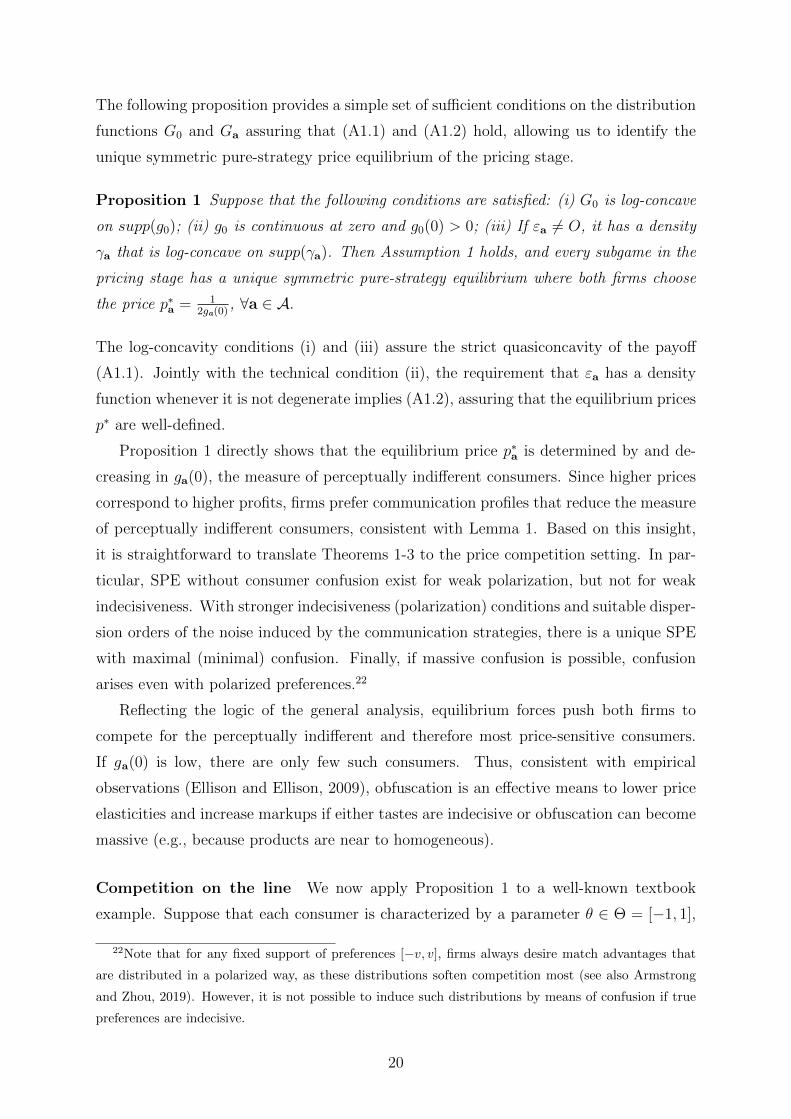
Competition on the line We now apply Proposition 1 to a well-known textbook

example. Suppose that each consumer is characterized by a parameter θ ∈ Θ = [−1, 1],

22Note that for any fixed support of preferences [−v, v], firms always desire match advantages that

are distributed in a polarized way, as these distributions soften competition most (see also Armstrong

and Zhou, 2019). However, it is not possible to induce such distributions by means of confusion if true

preferences are indecisive.

20

which is drawn from a commonly known distribution H with zero-symmetric density

function h(θ) = αθ2 + 12− α

3on Θ, where α ∈

[−3

4, 6−3

√3

4

]. The true match value of a

type θ consumer for product i ∈ {1, 2} is vθi = µ − (xi − θ)2, where µ > 0 is sufficiently

large, and x1 = −1, x2 = 1 are the locations of the firms. Thus, θ can be interpreted

as the location of the consumer on a (Hotelling) line, where the true match value is

determined by a quadratic distance function. H translates into a distribution G0 of true

match advantages, where G0(x) = H(x4) ∀x ∈ R. If α > 0, the true match values are

strongly polarized on the support of G0, [−4, 4]. Conversely, if α < 0, the true match

values are strongly indecisive on [−4, 4]. More generally, |α| corresponds to the extent

of polarization or indecisiveness, respectively. To capture obfuscation, suppose that the

error distribution is uniformly distributed on an interval [−ωa, ωa] where ωa < 4 ∀a ∈ A,

i.e., confusion cannot be massive.

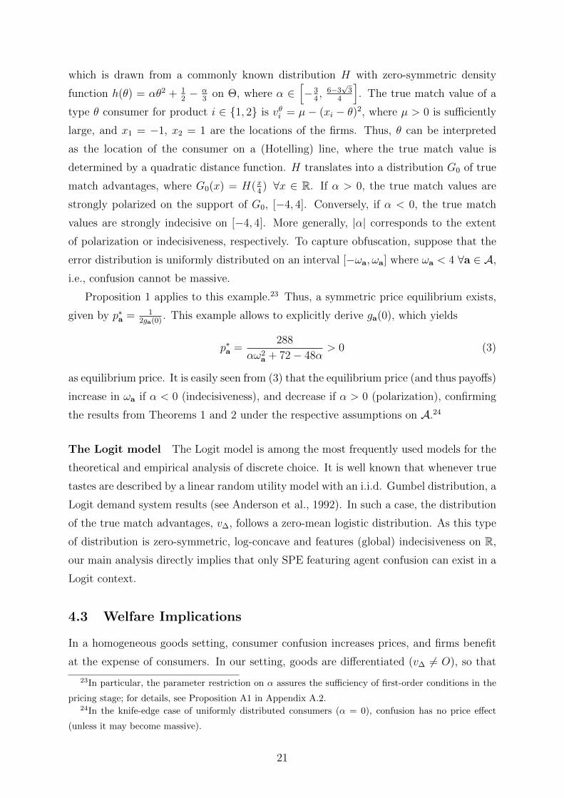
Proposition 1 applies to this example.23 Thus, a symmetric price equilibrium exists,

given by p∗a = 12ga(0)

. This example allows to explicitly derive ga(0), which yields

p∗a =288

αω2a + 72− 48α

> 0 (3)

as equilibrium price. It is easily seen from (3) that the equilibrium price (and thus payoffs)

increase in ωa if α < 0 (indecisiveness), and decrease if α > 0 (polarization), confirming

the results from Theorems 1 and 2 under the respective assumptions on A.24

The Logit model The Logit model is among the most frequently used models for the

theoretical and empirical analysis of discrete choice. It is well known that whenever true

tastes are described by a linear random utility model with an i.i.d. Gumbel distribution, a

Logit demand system results (see Anderson et al., 1992). In such a case, the distribution

of the true match advantages, v∆, follows a zero-mean logistic distribution. As this type

of distribution is zero-symmetric, log-concave and features (global) indecisiveness on R,

our main analysis directly implies that only SPE featuring agent confusion can exist in a

Logit context.

4.3 Welfare Implications

In a homogeneous goods setting, consumer confusion increases prices, and firms benefit

at the expense of consumers. In our setting, goods are differentiated (v∆ 6= O), so that

23In particular, the parameter restriction on α assures the sufficiency of first-order conditions in the

pricing stage; for details, see Proposition A1 in Appendix A.2.24In the knife-edge case of uniformly distributed consumers (α = 0), confusion has no price effect

(unless it may become massive).

21

consumer confusion could, in principle, reduce prices. However, in such a case (when pref-

erences are polarized), firms avoid obfuscating the market according to Theorems 1 and

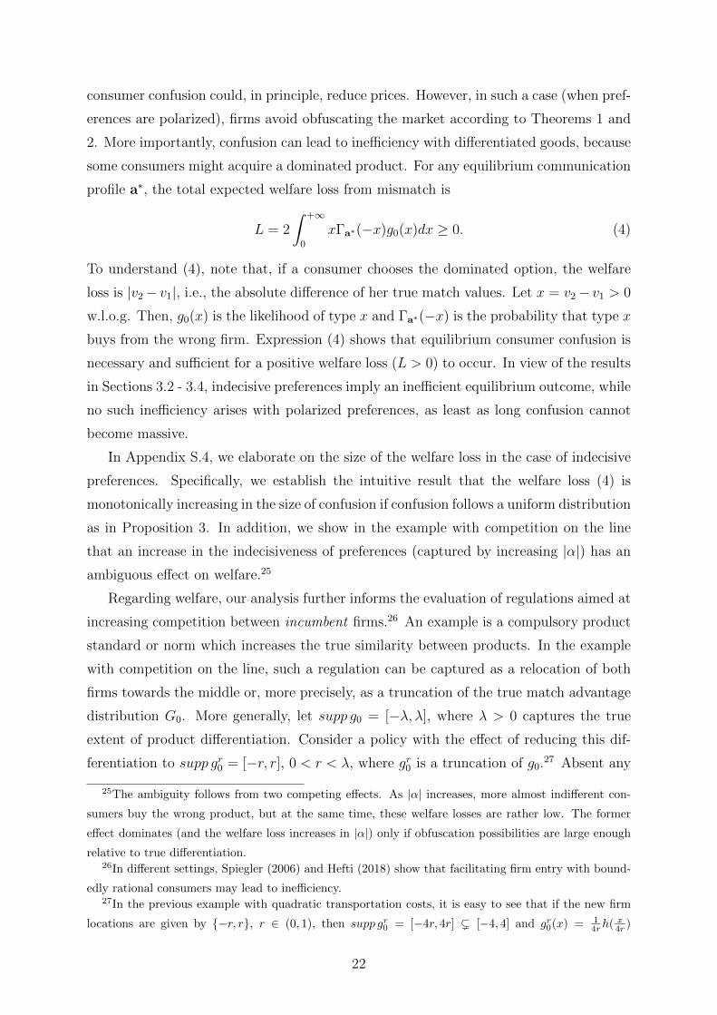
2. More importantly, confusion can lead to inefficiency with differentiated goods, because

some consumers might acquire a dominated product. For any equilibrium communication

profile a∗, the total expected welfare loss from mismatch is

L = 2

∫ +∞

0

xΓa∗(−x)g0(x)dx ≥ 0. (4)

To understand (4), note that, if a consumer chooses the dominated option, the welfare

loss is |v2− v1|, i.e., the absolute difference of her true match values. Let x = v2− v1 > 0

w.l.o.g. Then, g0(x) is the likelihood of type x and Γa∗(−x) is the probability that type x

buys from the wrong firm. Expression (4) shows that equilibrium consumer confusion is

necessary and sufficient for a positive welfare loss (L > 0) to occur. In view of the results

in Sections 3.2 - 3.4, indecisive preferences imply an inefficient equilibrium outcome, while

no such inefficiency arises with polarized preferences, as least as long confusion cannot

become massive.

In Appendix S.4, we elaborate on the size of the welfare loss in the case of indecisive

preferences. Specifically, we establish the intuitive result that the welfare loss (4) is

monotonically increasing in the size of confusion if confusion follows a uniform distribution

as in Proposition 3. In addition, we show in the example with competition on the line

that an increase in the indecisiveness of preferences (captured by increasing |α|) has an

ambiguous effect on welfare.25

Regarding welfare, our analysis further informs the evaluation of regulations aimed at

increasing competition between incumbent firms.26 An example is a compulsory product

standard or norm which increases the true similarity between products. In the example

with competition on the line, such a regulation can be captured as a relocation of both

firms towards the middle or, more precisely, as a truncation of the true match advantage

distribution G0. More generally, let supp g0 = [−λ, λ], where λ > 0 captures the true

extent of product differentiation. Consider a policy with the effect of reducing this dif-

ferentiation to supp gr0 = [−r, r], 0 < r < λ, where gr0 is a truncation of g0.27 Absent any

25The ambiguity follows from two competing effects. As |α| increases, more almost indifferent con-

sumers buy the wrong product, but at the same time, these welfare losses are rather low. The former

effect dominates (and the welfare loss increases in |α|) only if obfuscation possibilities are large enough

relative to true differentiation.26In different settings, Spiegler (2006) and Hefti (2018) show that facilitating firm entry with bound-

edly rational consumers may lead to inefficiency.27In the previous example with quadratic transportation costs, it is easy to see that if the new firm

locations are given by {−r, r}, r ∈ (0, 1), then supp gr0 = [−4r, 4r] ( [−4, 4] and gr0(x) = 14rh( x4r )

22

consumer confusion, it is easy to see that such a regulation successfully lowers equilib-

rium prices, as gr0(0) > g0(0), independent of the shape of g0. The following result shows

that, depending on consumer preferences, such regulations may have unintended, adverse

effects on welfare due to consumer confusion.28

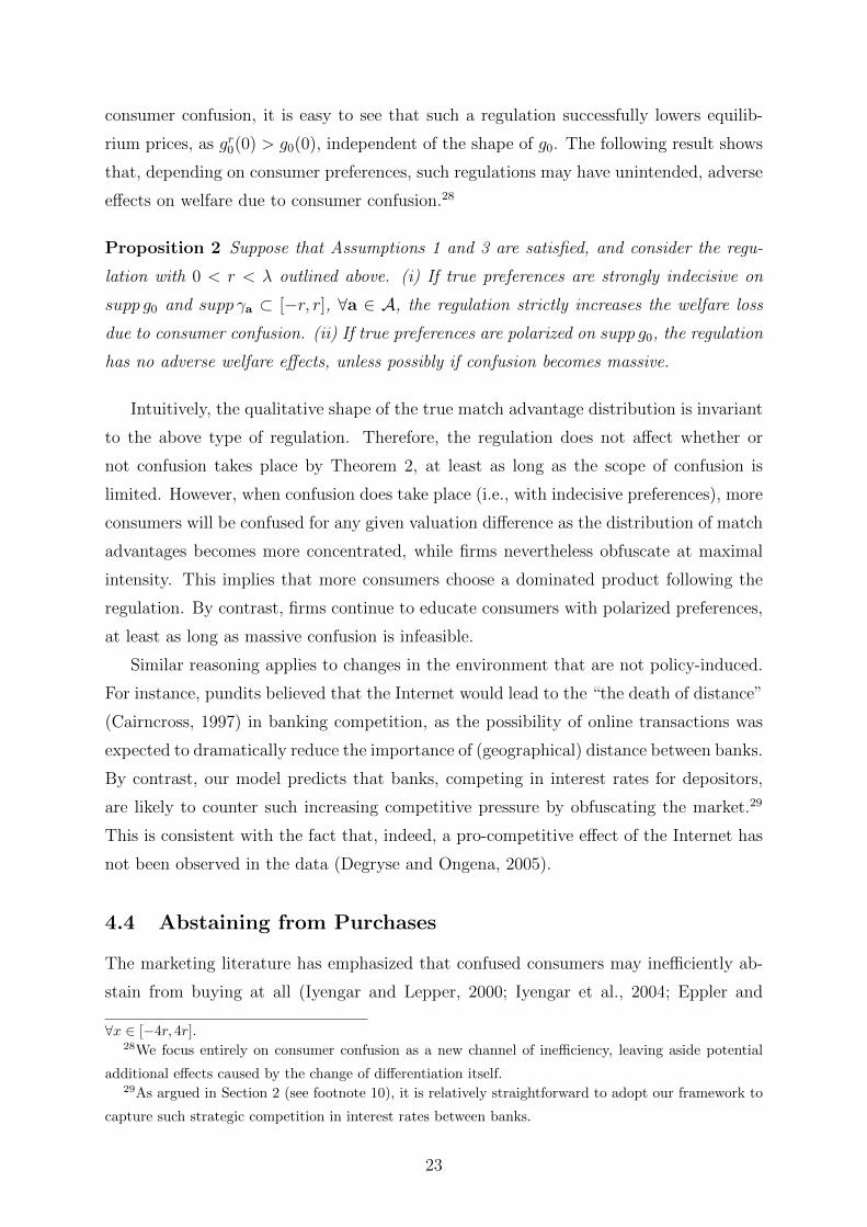
Proposition 2 Suppose that Assumptions 1 and 3 are satisfied, and consider the regu-

lation with 0 < r < λ outlined above. (i) If true preferences are strongly indecisive on

supp g0 and supp γa ⊂ [−r, r], ∀a ∈ A, the regulation strictly increases the welfare loss

due to consumer confusion. (ii) If true preferences are polarized on supp g0, the regulation

has no adverse welfare effects, unless possibly if confusion becomes massive.

Intuitively, the qualitative shape of the true match advantage distribution is invariant

to the above type of regulation. Therefore, the regulation does not affect whether or

not confusion takes place by Theorem 2, at least as long as the scope of confusion is

limited. However, when confusion does take place (i.e., with indecisive preferences), more

consumers will be confused for any given valuation difference as the distribution of match

advantages becomes more concentrated, while firms nevertheless obfuscate at maximal

intensity. This implies that more consumers choose a dominated product following the

regulation. By contrast, firms continue to educate consumers with polarized preferences,

at least as long as massive confusion is infeasible.

Similar reasoning applies to changes in the environment that are not policy-induced.

For instance, pundits believed that the Internet would lead to the “the death of distance”

(Cairncross, 1997) in banking competition, as the possibility of online transactions was

expected to dramatically reduce the importance of (geographical) distance between banks.

By contrast, our model predicts that banks, competing in interest rates for depositors,

are likely to counter such increasing competitive pressure by obfuscating the market.29

This is consistent with the fact that, indeed, a pro-competitive effect of the Internet has

not been observed in the data (Degryse and Ongena, 2005).

4.4 Abstaining from Purchases

The marketing literature has emphasized that confused consumers may inefficiently ab-

stain from buying at all (Iyengar and Lepper, 2000; Iyengar et al., 2004; Eppler and

∀x ∈ [−4r, 4r].28We focus entirely on consumer confusion as a new channel of inefficiency, leaving aside potential

additional effects caused by the change of differentiation itself.29As argued in Section 2 (see footnote 10), it is relatively straightforward to adopt our framework to

capture such strategic competition in interest rates between banks.

23

Mengis, 2004; Bertrand et al., 2010; Chernev et al., 2015).30 Consistent with this empiri-

cal observation, we next show that in the presence of binding outside options, firms may

choose a confusing communication strategy even though this induces some consumers

to exit the market. This provides an additional rationale for why the market does not

eliminate confusion and its negative consequences.

In the spirit of the Hotelling model, suppose that the perceived match values are

given by v1 = 1 + υ2

+ ε2

and v2 = 1 − υ2− ε

2, where υ ∈ [−1, 1] is governed by a zero-

symmetric distribution G0 with density g0. Further, all consumers have a reservation

value normalized to zero. Thus, a consumer purchases the good with the higher perceived

net value vj − pj if this net value is non-negative, and does not purchase otherwise.31

Compared to the previous analysis, each firm must take into account that a price increase

may now come at the additional cost of losing some consumers to whom the firm actually

is offering the better deal. The threat of exiting consumers becomes pertinent if prices

are high. Therefore it is conceivable that the possibility of a binding outside option may

discipline firms against obfuscating too much, e.g., in case of indecisive preferences.

In the following, we explain the main equilibrium patterns predicted by the above

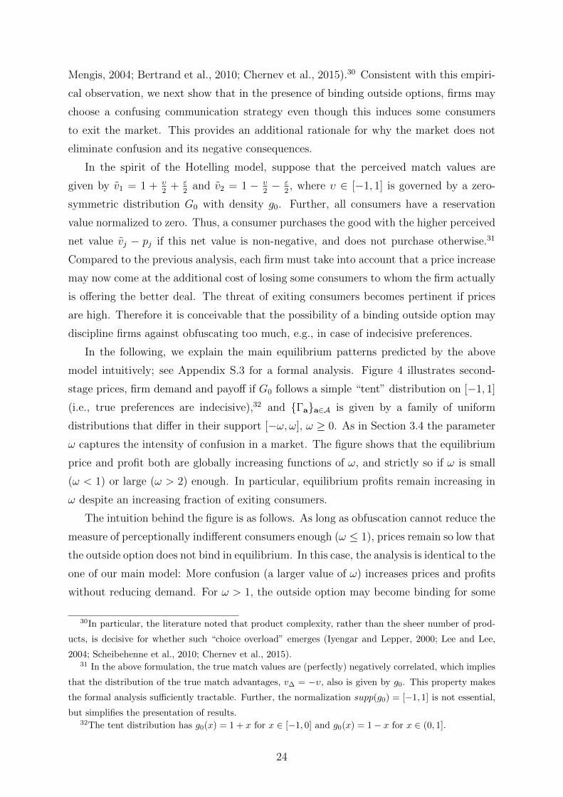
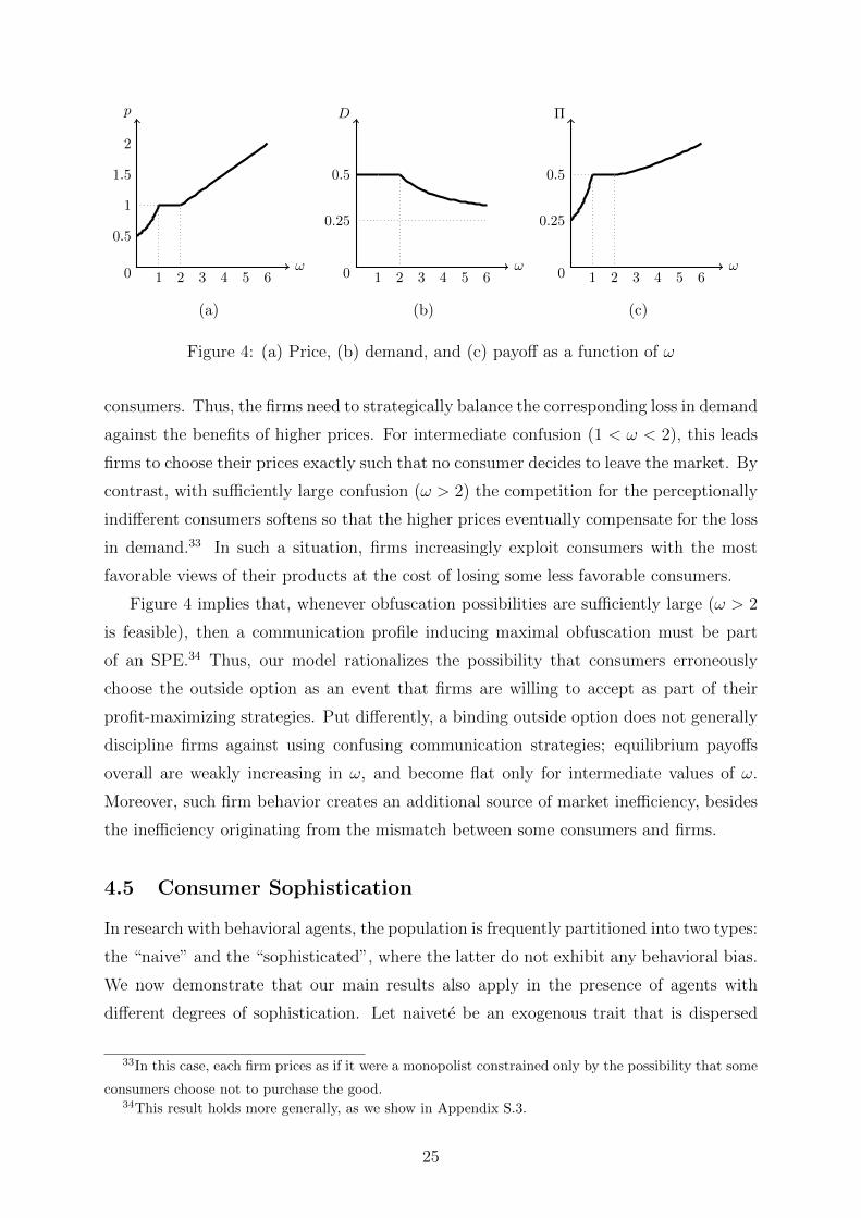
model intuitively; see Appendix S.3 for a formal analysis. Figure 4 illustrates second-

stage prices, firm demand and payoff if G0 follows a simple “tent” distribution on [−1, 1]

(i.e., true preferences are indecisive),32 and {Γa}a∈A is given by a family of uniform

distributions that differ in their support [−ω, ω], ω ≥ 0. As in Section 3.4 the parameter

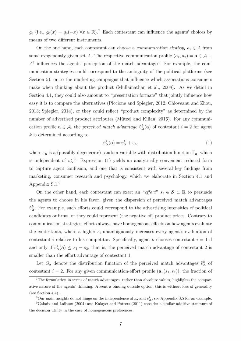
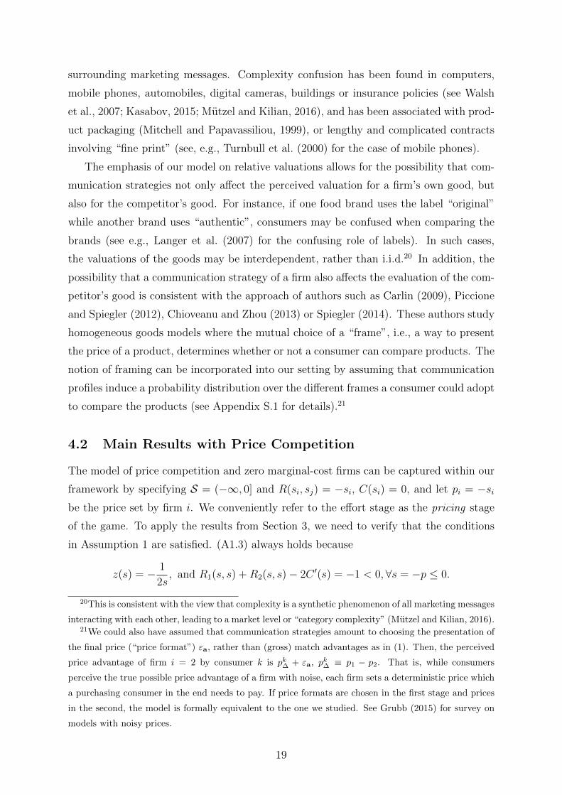
ω captures the intensity of confusion in a market. The figure shows that the equilibrium

price and profit both are globally increasing functions of ω, and strictly so if ω is small

(ω < 1) or large (ω > 2) enough. In particular, equilibrium profits remain increasing in

ω despite an increasing fraction of exiting consumers.

The intuition behind the figure is as follows. As long as obfuscation cannot reduce the

measure of perceptionally indifferent consumers enough (ω ≤ 1), prices remain so low that

the outside option does not bind in equilibrium. In this case, the analysis is identical to the

one of our main model: More confusion (a larger value of ω) increases prices and profits

without reducing demand. For ω > 1, the outside option may become binding for some

30In particular, the literature noted that product complexity, rather than the sheer number of prod-

ucts, is decisive for whether such “choice overload” emerges (Iyengar and Lepper, 2000; Lee and Lee,

2004; Scheibehenne et al., 2010; Chernev et al., 2015).31 In the above formulation, the true match values are (perfectly) negatively correlated, which implies

that the distribution of the true match advantages, v∆ = −υ, also is given by g0. This property makes

the formal analysis sufficiently tractable. Further, the normalization supp(g0) = [−1, 1] is not essential,

but simplifies the presentation of results.32The tent distribution has g0(x) = 1 + x for x ∈ [−1, 0] and g0(x) = 1− x for x ∈ (0, 1].

24

p

0

0.5

1

1.5

2

ω642 531

(a)

D

0

0.5

0.25

ω642 531

(b)

Π

0

0.5

0.25

ω642 531

(c)

Figure 4: (a) Price, (b) demand, and (c) payoff as a function of ω

consumers. Thus, the firms need to strategically balance the corresponding loss in demand

against the benefits of higher prices. For intermediate confusion (1 < ω < 2), this leads

firms to choose their prices exactly such that no consumer decides to leave the market. By

contrast, with sufficiently large confusion (ω > 2) the competition for the perceptionally

indifferent consumers softens so that the higher prices eventually compensate for the loss

in demand.33 In such a situation, firms increasingly exploit consumers with the most

favorable views of their products at the cost of losing some less favorable consumers.

Figure 4 implies that, whenever obfuscation possibilities are sufficiently large (ω > 2

is feasible), then a communication profile inducing maximal obfuscation must be part

of an SPE.34 Thus, our model rationalizes the possibility that consumers erroneously

choose the outside option as an event that firms are willing to accept as part of their

profit-maximizing strategies. Put differently, a binding outside option does not generally

discipline firms against using confusing communication strategies; equilibrium payoffs

overall are weakly increasing in ω, and become flat only for intermediate values of ω.

Moreover, such firm behavior creates an additional source of market inefficiency, besides

the inefficiency originating from the mismatch between some consumers and firms.

4.5 Consumer Sophistication

In research with behavioral agents, the population is frequently partitioned into two types:

the “naive” and the “sophisticated”, where the latter do not exhibit any behavioral bias.

We now demonstrate that our main results also apply in the presence of agents with

different degrees of sophistication. Let naivete be an exogenous trait that is dispersed

33In this case, each firm prices as if it were a monopolist constrained only by the possibility that some

consumers choose not to purchase the good.34This result holds more generally, as we show in Appendix S.3.

25

over the consumer population according to the random variable ρ, such that v∆(a) =

v∆ + ρεa, where supp ρ ⊂ [0, 1], and ρ, v∆ and εa are independent for any given a ∈A. A consumer with ρ = 0 is fully sophisticated, meaning that her perceptions are

unaffected by the chosen communication strategies: v∆(a) = v∆ ∀a ∈ A. By contrast,

a larger value of ρ means less sophistication in that the possible distortions induced by

εa are amplified.35 Alternatively, ρ can be seen as a measure for the level of “confusion

proneness” as introduced by Walsh et al. (2007), capturing that different consumers may

be differ in how susceptible they are to obfuscation techniques. It is straightforward to

use first-order conditions to verify that p∗a = 12ga(0)

results in the pricing stage, where

ga(0) =∫ ∫

g0(ρε)dΓa(ε)dΓρ(ρ) and Γρ denotes the distribution function of ρ.36 It is

evident from this expression that the main firm-side incentives to obfuscate or educate

still depend exclusively on the shape of g0.37

4.6 Relation to the Advertising Literature

One interpretation of our results is that more precise information about the products

increases prices and profits with indecisive preferences, but decreases them with polar-

ized preferences. This contrasts with familiar results from the literature on informative

advertising, surveyed in Bagwell (2007), where more information provided by firms typi-

cally reduces prices by intensifying competition. Our paper also relates to the literature

on persuasive advertising, which emphasizes that persuasive advertising games have the

structure of a prisoners’ dilemma: Firms engage in costly advertising races, which, in

equilibrium, do not affect prices and gross profits (see, e.g., Dixit and Norman, 1978;

Von der Fehr and Stevik, 1998; Bagwell, 2007). In our setting, obfuscating communica-

tion strategies can be interpreted as activities that persuade some consumers at the cost

of alienating others.38 Our analysis shows that firms either refrain from such advertising

measures (with polarized consumers) or use the measures to soften competition (with

35The information may be so complex that it cannot be fully assessed even by sophisticated agents

(Eichenberger and Serna, 1996), in which case ρ > 0.36The typical case of binary types occurs if all probability mass of Γρ rests on ρ = 0 and ρ = 1, which

yields ga(0) = Γρ(0)ga(0) + (1− Γρ(0))g0(0).37In our framework, naive consumers impose a negative externality on sophisticated ones, independent

of the shape of the preference distribution. This is because, in any case, the equilibrium measures taken by

firms are such as to either confuse or educate the naive consumers, which increases the equilibrium price

for sophisticated consumers as well. In fact, the desire for consumer education of firms and sophisticated

consumers are exactly antipodal to each other.38As an example, consider the cold-calls of tele-marketing agents (see Schumacher and Thysen, 2017).

26

indecisive consumers), which contrasts with the prisoners’ dilemma situations.39

Finally, our results are related to Johnson and Myatt (2006), who show that a monop-

olist does not necessarily want to engage in measures related to advertising, marketing or

product design that increase the heterogeneity of consumer valuations. In their monopoly

analysis, the entire distribution of valuations matters for the optimal pricing strategy of

a monopolist, while in our setting, in the absence of outside options the competitive

forces imply that equilibrium prices depend only on the mass of perceptually indifferent

consumers. Firms always desire more consumer heterogeneity in the sense of fewer indif-

ferent and hence highly price-sensitive consumers. Our main result that the shape of the

true match advantage distribution determines whether such heterogeneity is achievable

by means of obfuscation or education has no counterpart in Johnson and Myatt (2006).

5 Competition for Voters

Communication strategies play a major role in political competition. A substantial liter-

ature has asked why political candidates often choose ambiguous platforms, rather than

describe their policies exactly. In the standard Hotelling-Downs framework of political

competition, ambiguous platforms indeed are always suboptimal when voters are risk-

averse (Shepsle, 1972). By contrast, some authors have argued that ambiguity may be

preferable, e.g., because it allows political candidates to maintain the flexibility to adapt

to future circumstances (Aragones and Neeman, 2000; Kartik et al., 2017), while others

have provided behavioral explanations, relying on context-dependent preferences (Callan-

der and Wilson, 2008) or projection bias (Jensen, 2009).We contribute to the literature

on strategic ambiguity in political competition by studying how the incentives of political

candidates to confuse or educate potential voters about their platforms depend on the

heterogeneity of true voter preferences. In Section 5.1, we directly apply our general

analysis to the case of symmetric candidates. In Section 5.2, we relax the assumptions of

perfectly symmetric contestants and unbiased perception errors.

5.1 Symmetric Political Parties

We consider the specification of the general model with R(s1, s2) = 1 and C(si) = ksηi ,

∀s1, s2 ∈ S = R+, where k > 0 and η > 1. Here, we interpret the market share as

the share of votes, and we assume that the two political contestants, henceforth simply

referred to as “parties”, value the votes symmetrically. Parties are heterogeneous with

39It is easy to show that our results would qualitatively apply if we introduced obfuscation costs.

27

respect to their ideology, and voters have heterogeneous preferences over policies, captured

by the distribution G0 of true match advantages. Voters evaluate a party according to

their perceived match advantages. The distribution of perceived match advantages, Ga, is

determined by the parties’ communication strategies (a1, a2).40 In particular, a party can

avoid being precise, leading to a noisy perception, whereby some voters get a too positive

impression of the party’s value for them and others get a too negative impression. Parties

not only influence election outcomes by their platforms. In addition, it is well known that

the prominence in the media of a party has a strong persuasive effect on voting behavior.

For instance, a candidate’s comparative advantage in media exposure can lead undecided

voters to favor him (Gerber et al., 2011; Gallego and Schofield, 2017). We capture this

observation by interpreting si as advertising efforts, where the party with si > sj is more

prominent and, consequently, wins more undecided voters.

Contrary to price reductions, efforts in this setting are unconditional, that is, they

arise independent of the contestants’ success in attracting market share. Nevertheless, our

main insights about how the chosen communication strategies relate to the true dispersion

of preferences carry over to political competition. Under suitable parameter restrictions

(see Appendix A2), the equilibrium effort level s∗a is described by the first-order equilib-

rium equation ga(0) = C ′(s∗a). Hence, s∗a is strictly increasing and equilibrium payoffs

are strictly decreasing in the mass of perceptually indifferent voters ga(0), reflecting in-

creasing equilibrium effort levels and advertising expenditures .41 Both parties therefore

have a clear incentive to evade such intense competition. If Assumptions 2 and 3 hold,

candidates will choose ambiguous platforms if preferences are indecisive (but not if they

are polarized). In other words, a situation with indecisive preferences, i.e., with many

truly undecided voters, provides a breeding ground for voter confusion.

5.2 Asymmetric Contestants

While our model allows for ex-post asymmetry of the contestants (after the choice of

efforts), it assumes that they are symmetric ex ante (before the choice of communication

strategies) and ex interim (between the choices of communication and efforts). We next

elaborate on the robustness of the main insights of our paper with respect to these

40We can use higher values of ai to capture greater ambiguity due to, for example, a larger set

of policies (which leads to a larger support of the perceived match advantages), as is common in the

literature.41This is a special case of Lemma 1. We formally show in Appendix A.3 (see Proposition A2) that a

symmetric equilibrium in the effort stage exists whenever the cost function is sufficiently convex (i.e., η

is sufficiently large).

28

v-v

𝑔𝑔0

𝑔𝑔𝒂𝒂

𝑠𝑠∆′ 𝑠𝑠∆ v-v

𝐺𝐺0

𝐺𝐺𝒂𝒂(𝑠𝑠∆′)

𝑠𝑠∆′ 𝑠𝑠∆

1/2

𝐺𝐺0(𝑠𝑠∆)

𝐺𝐺𝒂𝒂

Figure 5: The effects of confusion with ex-ante asymmetric contestants indecisiveness

symmetry assumptions in the context of the voting model; similar reasoning applies to

the price competition case.

Ex-ante asymmetry We first show that, with ex-ante asymmetric contestants, the

shape of preferences has a similar effect on the nature of equilibrium as in the symmetric

case. Suppose that i = 1 is a strong and i = 2 a weak contestant in the sense that

C ′1(s) < C ′2(s) for any s > 0. For a given distribution of perceived match advantages

Ga, the first-order conditions in the effort stage yield ga(s1 − s2) = C ′1(s1) = C ′2(s2),

showing that marginal costs are equated by equilibrium forces. It follows that we must

have s1 − s2 ≡ s∆ > 0 in equilibrium, reflecting the advantage of the strong contestant.

Because then also Ga(s∆) > 1/2, it follows that, despite unbiased perception errors,

communication can lead to a redistribution of market shares and thereby possibly induce

a conflict of interests between the contestants. Figure 5 illustrates the effects of agent

confusion for indecisive preferences.42

As captured in the left part of Figure 5, agent confusion spreads out the density of

the perceived match values ga below g0, and accordingly rotates the distribution Ga at 0

clockwise (displayed in the right part of Figure 5). On the one hand, both contestants

benefit from confusion because the downward shift of ga softens competition and allows

them to choose lower equilibrium efforts. On the other hand, as we can see from the

right part of Figure 5, the market share of the strong (weak) contestant would be larger

(smaller) without agent confusion. Therefore, the strong contestant may have a mixed

view about the benefits of agent confusion, while the weak contestant can only benefit.43

The opposite logic applies with polarized preferences. Then, agent confusion can only

harm the weak contestant because it intensifies competition, and the weak contestant

loses some otherwise favorable agents to the strong competitor. In sum, the weak com-

42The suggestive insights portrayed by Figure 5 are supported by formal results (see Appendix S.6).43Kalaycı and Potters (2011) observe a similar result in a Hotelling model with quality-differentiated

products; also see Gabaix and Laibson (2004).

29

petitor unambiguously strives to educate (to confuse) in the case of polarized (indecisive)

preferences, while the incentive is less clear-cut for the strong contestant.44

Ex-interim asymmetry Despite the many reasons suggesting an unbiased nature of

the perception errors in the voters’ comparison, the existence of communication profiles

that lead to biased comparisons is conceivable. Are such biased communication profiles

played in equilibrium provided that they are available? Do they overthrow the role of

preferences that we identified in our previous results?45 We study these questions in

Appendix S.7 in a simple extension with binary communication strategies A = {0, 1},where aj = 0 corresponds to accurate communication, and aj = 1 to communication that

leads to noisy but biased comparisons in j’s favor given that a−j = 0. Preferences still play

a key role for whether education or confusion results with possibly biased communication

profiles: Mutual obfuscation remains the unique equilibrium with indecisive preferences,

while education remains the only equilibrium outcome with polarized preferences if the

contestants can unilaterally educate the agents, e.g., as in Heidhues et al. (2016).46

6 Conclusion

Our paper provides a theory explaining the strategic use of confusion by contestants,

such as firms or political parties, who compete for agents with heterogeneous preferences.

We find that the distribution of true agent preferences plays a decisive role for whether

contestants choose an educating or a confusing communication strategy. Agent education

emerges as an equilibrium outcome if true preferences are polarized, intuitively meaning

that tastes are concentrated near the contestants’ positions. By contrast, confusion arises

for the case of indecisive preferences, characterized by a concentration of agents who are

truly indifferent between the choice alternatives.

We also find that confusion can be an equilibrium outcome if it can be massive in the

sense that the dispersion of true preferences is narrow relative to the perception errors that

44It is easy to see that a similar result emerges if C1(s) = C2(s) but g0 is shifted to the right, such

that with equal effort, contestant i = 1 would obtain a strictly larger market share.45Clearly, these issues are relevant for the price competition application as well: For instance, if

Duracel’s advertises its batteries as the “longest-living batteries”, then all other batteries must be short-

lived. If sufficiently many consumers are influenced by this logic, then this would be a clear case of biased

communication.46If education cannot be forced unilaterally, two possibilities arise. With very large biases, obfuscation

becomes so attractive that contestants are trapped in a Prisoner’s Dilemma, with mutual obfuscation

as the sole equilibrium outcome. For biases of intermediate size, a coordination game results with two

asymmetric equilibria, where exactly one firm obfuscates.

30

can be induced by obfuscation. In a product market setting with differentiated products,

this generalizes the central insight from behavioral industrial organization that firms

in homogeneous goods industries seek to obfuscate to escape the Bertrand trap: With

homogeneous goods any confusion must be massive in our sense. Our analysis shows that,

other than with homogeneous goods, firms do not always choose to confuse consumers,

but if they do, its welfare effects are more detrimental. In particular, consumers can

be harmed by choosing dominated options, paying higher prices or inefficiently forgoing

purchases. The latter may help to understand why the consumer decision not to purchase

any option due to confusion is a persistent empirical phenomenon.

Regulatory interventions may lead to undesired outcomes for reasons related to pref-

erence heterogeneity. For instance, regulations aiming at increasing the similarity of

products to foster competition may be inefficient, because they can end up fostering

confusion instead. Further, general restrictions of the acceptable communication strate-

gies may backfire in situations with polarized preferences, where, in the absence of such

restrictions, contestants would choose their communication to dissolve any pre-existing

agent confusion.

Applied to political competition, our analysis shows that the distribution of voter

preferences crucially affects whether parties choose ambiguous platforms: With many

undecided voters such ambiguity may help to soften political competition as it moves

the perceived valuations for the candidates towards polarization. At the same time,

we find that, with pre-existing polarization, parties prefer to educate voters about their

platforms. In sum, we find that the dispersion of preferences has similar implications for

the incentives to confuse or educate in (political) contests or market competition with

differentiated products.

31

References

Anderson, S. P., A. De Palma, and J. F. Thisse (1992): Discrete Choice Theory of

Product Differentiation, MIT Press.

Aragones, E. and Z. Neeman (2000): “Strategic ambiguity in electoral competition,” Jour-

nal of Theoretical Politics, 12, 183–204.

Armstrong, M. and J. Zhou (2019): “Consumer information and the limits to competition,”

Working paper.

Bagnoli, M. and T. Bergstrom (2005): “Log-concave probability and its applications,”

Economic Theory, 26, 445–469.

Bagwell, K. (2007): “The economic analysis of advertising,” in Handbook of Industrial Or-

ganization, ed. by M. Armstrong and R. Porter, Elsevier, vol. 3, chap. 28, 1701–1844.

Bertrand, M., D. Karlan, S. Mullainathan, E. Shafir, and J. Zinman (2010):

“What’s advertising content worth? Evidence from a consumer credit marketing field ex-

periment,” The Quarterly Journal of Economics, 125, 263–306.

Cairncross, F. (1997): The Death of Distance: How the Communications Revolution Will

Change Our Lives, Harvard Business School Press.

Callander, S. and C. H. Wilson (2008): “Context-dependent voting and political ambigu-

ity,” Journal of Public Economics, 92, 565–581.

Caplin, A. and M. Dean (2015): “Revealed preference, rational inattention, and costly

information acquisition,” American Economic Review, 105, 2183–2203.

Carlin, B. I. (2009): “Strategic price complexity in retail financial markets,” Journal of

Financial Economics, 91, 278–287.

Chernev, A., U. Bockenholt, and J. Goodman (2015): “Choice overload: A conceptual

review and meta-analysis,” Journal of Consumer Psychology, 25, 333–358.

Chioveanu, I. and J. Zhou (2013): “Price competition with consumer confusion,” Manage-

ment Science, 59, 2450–2469.

Degryse, H. and S. Ongena (2005): “Distance, lending relationships, and competition,”

The Journal of Finance, 60, 231–266.

Dixit, A. and V. Norman (1978): “Advertising and welfare,” The Bell Journal of Economics,

9, 1–17.

Downs, A. (1957): An Economic Theory of Democracy, New York: Harper.

Eichenberger, R. and A. Serna (1996): “Random errors, dirty information, and politics,”

Public Choice, 86, 137–156.

32

Eliaz, K. and R. Spiegler (2011a): “Consideration sets and competitive marketing,” Reviews

of Economic Studies, 78, 235–262.

——— (2011b): “On the strategic use of attention grabbers,” Theoretical Economics, 6, 127–

155.

Ellison, G. and S. F. Ellison (2009): “Search, obfuscation, and price elasticities on the

internet,” Econometrica, 77, 427–452.

Ellison, G. and A. Wolitzky (2012): “A search cost model of obfuscation,” The RAND

Journal of Economics, 43, 417–441.

Eppler, M. J. and J. Mengis (2004): “The concept of information overload: A review of

literature from organization science, accounting, marketing, MIS, and related disciplines,”

The Information Society, 20, 325–344.

Franklin, C. H. (1991): “Eschewing obfuscation? Campaigns and the perception of US

Senate incumbents,” American Political Science Review, 85, 1193–1214.

Freixas, X. and J.-C. Rochet (2008): Microeconomics of Banking, MIT press.

Gabaix, X. and D. Laibson (2004): “Competition and consumer confusion,” Working paper.

——— (2006): “Shrouded attributes, consumer myopia, and information suppression in com-

petitive markets,” Quarterly Journal of Economics, 121, 505–540.

Gallego, M. and N. Schofield (2017): “Modeling the effect of campaign advertising on US

presidential elections when differences across states matter,” Mathematical Social Sciences,

90, 160–181.

Gerber, A. S., J. G. Gimpel, D. P. Green, and D. R. Shaw (2011): “How large and

long-lasting are the persuasive effects of televised campaign ads? Results from a randomized

field experiment,” American Political Science Review, 105, 135–150.

Gill, J. (2005): “An entropy measure of uncertainty in vote choice,” Electoral Studies, 24,

371–392.

Grossman, G. M. and C. Shapiro (1984): “Informative advertising with differentiated prod-

ucts,” Review of Economic Studies, 51, 63–81.

Grubb, M. D. (2015): “Failing to choose the best price: Theory, evidence, and policy,” Review

of Industrial Organization, 47, 303–340.

Haan, P. and C. Berkey (2002): “A study of the believability of the forms of puffery,”

Journal of Marketing Communications, 8, 243–256.

Hefti, A. (2017): “Equilibria in symmetric games: Theory and applications,” Theoretical

Economics, 12, 979–1002.

33

——— (2018): “Limited attention, competition and welfare,” Journal of Economic Theory,

178, 318–359.

Heidhues, P. and B. Koszegi (2017): “Naivete-based discrimination,” The Quarterly Journal

of Economics, 132, 1019–1054.

Heidhues, P., B. Koszegi, and T. Murooka (2016): “Inferior products and profitable

deception,” Review of Economic Studies, 84, 323–356.

Iyengar, S., G. Huberman, and W. Jiang (2004): “How much choice is too much? Con-

tributions to 401(k) retirement plans,” in Pension Design and Structure: New Lessons from

Behavioral Finance, ed. by O. Mitchell and S. Utkus, Oxford University Press, chap. 5, 83–96.

Iyengar, S. S. and M. R. Lepper (2000): “When choice is demotivating: Can one desire

too much of a good thing?” Journal of Personality and Social Psychology, 79, 995.

Jacobson, G. C. and J. L. Carson (2015): The Politics of Congressional Elections, Rowman

& Littlefield.

Jacoby, J. (1977): “Information load and decision quality: Some contested issues,” Journal

of Marketing Research, 14, 569–573.

Jensen, T. (2009): “Projection effects and strategic ambiguity in electoral competition,” Public

Choice, 141, 213–232.

Johnson, J. P. and D. P. Myatt (2006): “On the simple economics of advertising, marketing,

and product design,” American Economic Review, 96, 756–784.

Kalaycı, K. and J. Potters (2011): “Buyer confusion and market prices,” International

Journal of Industrial Organization, 29, 14–22.

Kamenica, E. and M. Gentzkow (2011): “Bayesian persuasion,” American Economic Re-

view, 101, 2590–2615.

Kartik, N., R. Van Weelden, and S. Wolton (2017): “Electoral ambiguity and political

representation,” American Journal of Political Science, 61, 958–970.

Kasabov, E. (2015): “What we know, don’t know, and should know about confusion market-

ing,” European Journal of Marketing, 49, 1777–1808.

Langer, A., M. Eisend, and A. Ku (2007): “The impact of eco-labels on consumers: less

information, more confusion?” in European Advances in Consumer Research, ed. by M. A. M.

S. Borghini and C. Otnes, Duluth, MN: Association for Consumer Research, vol. 8, 338–339.

Lee, B.-K. and W.-N. Lee (2004): “The effect of information overload on consumer choice

quality in an on-line environment,” Psychology & Marketing, 21, 159–183.

Leek, S., I. Szmigin, and E. Baker (2015): “Consumer confusion and front of pack (FoP)

nutritional labels,” Journal of Customer Behavior, 14, 49–61.

34

Loewenstein, G., J. Y. Friedman, B. McGill, S. Ahmad, S. Linck, S. Sinkula,

J. Beshears, J. J. Choi, J. Kolstad, D. Laibson, B. C. Madrian, J. A. List, and

K. G. Volpp (2013): “Consumers misunderstanding of health insurance,” Journal of Health

Economics, 32, 850–862.

Malhotra, N. K. (1982): “Information load and consumer decision making,” Journal of

Consumer Research, 8, 419–430.

Miller, G. A. (1956): “The magical number seven, plus or minus two: some limits on our

capacit for processing information,” Psychological Review, 63, 81–97.

Mitchell, V.-W. and I. Kearney (2002): “A critique of legal measures of brand confusion,”

Journal of Product and Brand Management, 11, 357–379.

Mitchell, V.-W. and V. Papavassiliou (1999): “Marketing causes and implications of

consumer confusion,” Journal of Product and Brand Management, 8, 319–342.

Mullainathan, S., J. Schwartzstein, and A. Shleifer (2008): “Coarse thinking and

persuasion,” Quarterly Journal of Economics, 123, 577–619.

Muller, A. (1998): “Comparing risks with unbounded distributions,” Journal of Mathematical

Economics, 30, 229–239.

Murray, D. J. (1993): “A perspective for viewing the history of psychophysics,” Behavioral

and Brain Sciences, 16, 115–137.

Mutzel, L. M. A. and T. Kilian (2016): “Product complexity in consumer research: lit-

erature review and implications for future research,” in Rediscovering the Essentiality of

Marketing, ed. by L. Petruzzellis and R. S. Winer, Springer, 645–661.

Piccione, M. and R. Spiegler (2012): “Price competition under limited comparability,”

Quarterly Journal of Economics, 127, 97–135.

Rothschild, M. and J. E. Stiglitz (1970): “Increasing risk: I. A definition,” Journal of

Economic Theory, 2, 225–243.

Rovny, J. (2012): “Who emphasizes and who blurs? Party strategies in multidimensional

competition,” European Union Politics, 13, 269–292.

Rubin, H. and T. Sellke (1986): “On the distributions of sums of symmetric random vari-

ables and vectors,” The Annals of Probability, 14, 247–259.

Salop, S. (1979): “Monopolistic Competition with Outside Goods,” The Bell Journal of Eco-

nomics, 10, 141–156.

Scheibehenne, B., R. Greifeneder, and P. M. Todd (2010): “Can there ever be too

many options? A meta-analytic review of choice overload,” Journal of Consumer Research,

37, 409–425.

35

Schumacher, H. and H. Thysen (2017): “Equilibrium Contracts and Boundedly Rational

Expectations,” Mimeo.

Shepsle, K. A. (1972): “The strategy of ambiguity: Uncertainty and electoral competition,”

American Political Science Review, 66, 555–568.

Solomon, M. R., D. W. Dahl, K. White, J. L. Zaichkowsky, and R. Polegato (2014):

Consumer Behavior: Buying, Having, and Being, vol. 10, Pearson London.

Spiegler, R. (2006): “Competition over agents with boundedly rational expectations,” Theo-

retical Economics, 1, 207–231.

——— (2014): “Competitive framing,” American Economic Journal: Microeconomics, 6, 35–

58.

——— (2019): “Can agents with causal misperceptions be systematically fooled?” Journal of

the European Economic Association, forthcoming.

Tirole, J. (1988): The Theory of Industrial Organization, MIT press.

Tomz, M. and R. P. Van Houweling (2009): “The electoral implications of candidate

ambiguity,” American Political Science Review, 103, 83–98.

Turnbull, P. W., S. Leek, and G. Ying (2000): “Customer confusion: The mobile phone

market,” Journal of Marketing Management, 16, 143–163.

Von der Fehr, N.-H. M. and K. Stevik (1998): “Persuasive advertising and product

differentiation,” Southern Economic Journal, 113–126.

Walsh, G., T. Hennig-Thurau, and V.-W. Mitchell (2007): “Consumer confusion prone-

ness: scale development, validation, and application,” Journal of Marketing Management, 23,

697–721.

36

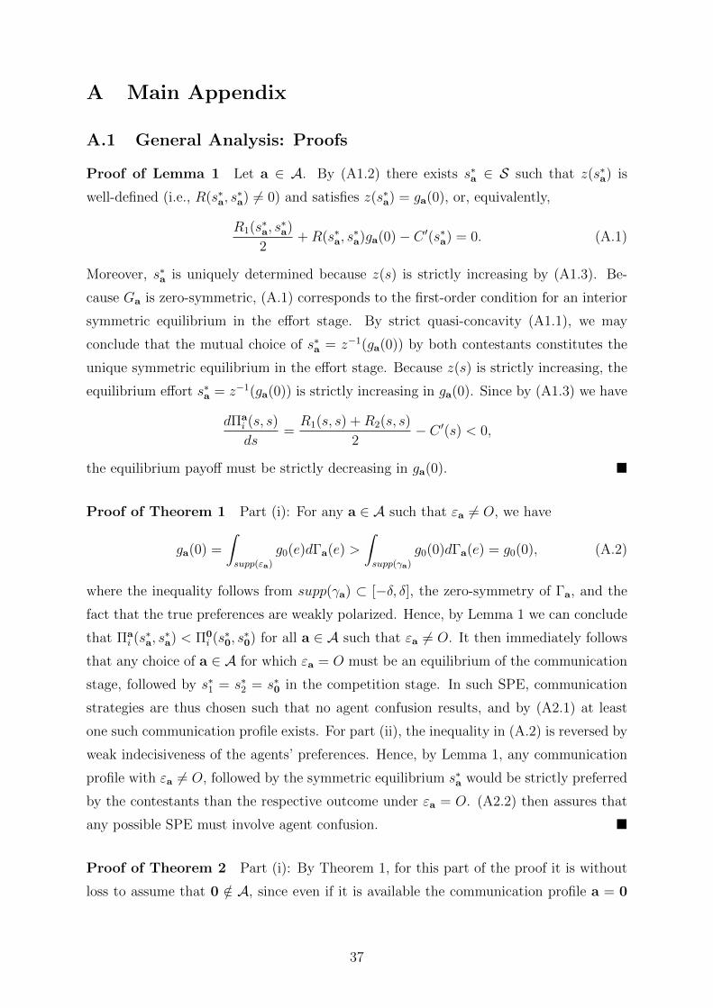
A Main Appendix

A.1 General Analysis: Proofs

Proof of Lemma 1 Let a ∈ A. By (A1.2) there exists s∗a ∈ S such that z(s∗a) is

well-defined (i.e., R(s∗a, s∗a) 6= 0) and satisfies z(s∗a) = ga(0), or, equivalently,

R1(s∗a, s∗a)

2+R(s∗a, s

∗a)ga(0)− C ′(s∗a) = 0. (A.1)

Moreover, s∗a is uniquely determined because z(s) is strictly increasing by (A1.3). Be-

cause Ga is zero-symmetric, (A.1) corresponds to the first-order condition for an interior

symmetric equilibrium in the effort stage. By strict quasi-concavity (A1.1), we may

conclude that the mutual choice of s∗a = z−1(ga(0)) by both contestants constitutes the

unique symmetric equilibrium in the effort stage. Because z(s) is strictly increasing, the

equilibrium effort s∗a = z−1(ga(0)) is strictly increasing in ga(0). Since by (A1.3) we have

dΠai (s, s)

ds=R1(s, s) +R2(s, s)

2− C ′(s) < 0,

the equilibrium payoff must be strictly decreasing in ga(0). �

Proof of Theorem 1 Part (i): For any a ∈ A such that εa 6= O, we have

ga(0) =

∫supp(εa)

g0(e)dΓa(e) >

∫supp(γa)

g0(0)dΓa(e) = g0(0), (A.2)

where the inequality follows from supp(γa) ⊂ [−δ, δ], the zero-symmetry of Γa, and the

fact that the true preferences are weakly polarized. Hence, by Lemma 1 we can conclude

that Πai (s∗a, s∗a) < Π0

i (s∗0, s∗0) for all a ∈ A such that εa 6= O. It then immediately follows

that any choice of a ∈ A for which εa = O must be an equilibrium of the communication

stage, followed by s∗1 = s∗2 = s∗0 in the competition stage. In such SPE, communication

strategies are thus chosen such that no agent confusion results, and by (A2.1) at least

one such communication profile exists. For part (ii), the inequality in (A.2) is reversed by

weak indecisiveness of the agents’ preferences. Hence, by Lemma 1, any communication

profile with εa 6= O, followed by the symmetric equilibrium s∗a would be strictly preferred

by the contestants than the respective outcome under εa = O. (A2.2) then assures that

any possible SPE must involve agent confusion. �

Proof of Theorem 2 Part (i): By Theorem 1, for this part of the proof it is without

loss to assume that 0 /∈ A, since even if it is available the communication profile a = 0

37

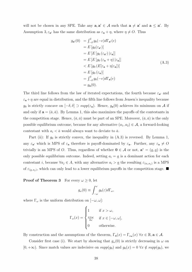
will not be chosen in any SPE. Take any a, a′ ∈ A such that a 6= a′ and a ≤ a′. By

Assumption 3, εa′ has the same distribution as εa + η, where η 6= O. Thus

ga′(0) =∫ δ−δ g0(−e)dΓa′(e)

= E [g0(εa′)]

= E [E [g0 (εa′) |εa]]

= E [E [g0 (εa + η) |εa]]

< E [g0 (E[εa + η|εa])]

= E [g0 (εa)]

=∫ δ−δ g0(−e)dΓa(e)

= ga(0).

(A.3)

The third line follows from the law of iterated expectations, the fourth because εa′ and

εa +η are equal in distribution, and the fifth line follows from Jensen’s inequality because

g0 is strictly concave on [−δ, δ] ⊃ supp(εa). Hence, ga(0) achieves its minimum on A if

and only if a = (a, a). By Lemma 1, this also maximizes the payoffs of the contestants in

the competition stage. Hence, (a, a) must be part of an SPE. Moreover, (a, a) is the only

possible equilibrium outcome, because for any alternative (a1, a2) ∈ A, a forward-looking

contestant with ai < a would always want to deviate to a.

Part (ii): If g0 is strictly convex, the inequality in (A.3) is reversed. By Lemma 1,

any εa′ which is MPS of εa therefore is payoff-dominated by εa. Further, any εa 6= O

trivially is an MPS of O. Thus, regardless of whether 0 ∈ A or not, a∗ = (a, a) is the

only possible equilibrium outcome. Indeed, setting ai = a is a dominant action for each

contestant i, because ∀aj ∈ A, with any alternative ai > a the resulting ε(ai,aj) is a MPS

of ε(a, aj), which can only lead to a lower equilibrium payoffs in the competition stage. �

Proof of Theorem 3 For every ω ≥ 0, let

gω(0) ≡∫ ω

−ωg0(ε)dΓω,

where Γω is the uniform distribution on [−ω, ω]:

Γω(x) =

1 if x > ω,

x+ω2ω

if x ∈ [−ω, ω],

0 otherwise.

By construction and the assumptions of the theorem, Γa(x) = Γωa(x) ∀x ∈ R, a ∈ A.

Consider first case (i). We start by showing that gω(0) is strictly decreasing in ω on

[0,+∞). Since match values are indecisive on supp(g0) and g0(x) = 0 ∀x /∈ supp(g0), we

38

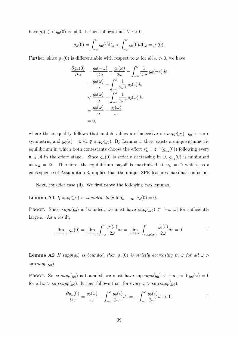
have g0(ε) < g0(0) ∀ε 6= 0. It then follows that, ∀ω > 0,

gω(0) =

∫ ω

−ωg0(ε)Γω <

∫ ω

−ωg0(0)dΓω = g0(0).

Further, since gω(0) is differentiable with respect to ω for all ω > 0, we have

∂gω(0)

∂ω=g0(−ω)

2ω+g0(ω)

2ω−∫ ω

−ω

1

2ω2g0(−ε)dε

=g0(ω)

ω−∫ ω

−ω

1

2ω2g0(ε)dε

<g0(ω)

ω−∫ ω

−ω

1

2ω2g0(ω)dε

=g0(ω)

ω− g0(ω)

ω

= 0,

where the inequality follows that match values are indecisive on supp(g0), g0 is zero-

symmetric, and g0(x) = 0 ∀x /∈ supp(g0). By Lemma 1, there exists a unique symmetric

equilibrium in which both contestants choose the effort s∗a = z−1(gωa(0)) following every

a ∈ A in the effort stage . Since gω(0) is strictly decreasing in ω, gωa(0) is minimized

at ωa = ω. Therefore, the equilibrium payoff is maximized at ωa = ω which, as a

consequence of Assumption 3, implies that the unique SPE features maximal confusion.

Next, consider case (ii). We first prove the following two lemmas.

Lemma A1 If supp(g0) is bounded, then limω→+∞ gω(0) = 0.

Proof. Since supp(g0) is bounded, we must have supp(g0) ⊂ [−ω, ω] for sufficiently

large ω. As a result,

limω→+∞

gω(0) = limω→+∞

∫ ω

−ω

g0(ε)

2ωdε = lim

ω→+∞

∫supp(g0)

g0(ε)

2ωdε = 0. �

Lemma A2 If supp(g0) is bounded, then gω(0) is strictly decreasing in ω for all ω >

sup supp(g0)

Proof. Since supp(g0) is bounded, we must have sup supp(g0) < +∞, and g0(ω) = 0

for all ω > sup supp(g0). It then follows that, for every ω > sup supp(g0),

∂gω(0)

∂ω=g0(ω)

ω−∫ ω

−ω

g0(ε)

2ω2dε = −

∫ ω

−ω

g0(ε)

2ω2dε < 0. �

39

Now consider any match value distribution that is polarized on its support supp(g0).

By definition, g0 is strictly decreasing on (inf supp(g0), 0] and is strictly increasing on

[0, sup supp(g0)). This implies that the support of g0 must be bounded, as otherwise we

would have ∫supp(g0)

g0(x)dx =

∫ +∞

−∞g0(x)dx ≥

∫ +∞

−∞g0(0)dx = +∞,

contradicting the definition of g0 as a density function. Applying Lemmas A1 and A2,

we can conclude that limω→+∞ gω(0) = 0 and that gω(0) is strictly decreasing in ω on

(supp(g0),+∞). Hence, given g0(0) > 0 there must exist ω > 0, such that if ω ≥ ω, then

gω(0) ≤ g0(0) and it is further decreasing as ω increases. Therefore, if ω is sufficiently

large, the subgame equilibrium payoff is maximized at ωa = ω which, by Assumption 3,

implies that the unique SPE then features maximal confusion. �

A.2 Price Competition: Proofs and Additional Results

Proof of Proposition 1 First, we argue that the log-concavity assumptions in (i) and

(iii) imply that each firm i’s expected payoff Πai (pi, pj) = piGa(pj − pi) is strictly quasi-

concave in pi, ∀a ∈ A and pj ≥ 0. To see this, first note that ∀a ∈ A, the distribution

function Ga, which is defined by

Ga(x) =

∫supp(εa)

G0(x− ε)dΓa(ε),∀x ∈ R,

is log-concave on supp(ga). This is trivial if εa = O, since in this case we have Ga = G0,

and G0 is log-concave on supp(g0) as condition (i) assumes. If εa 6= O, then by (iii) it has

a log-concave density γa, and we thus have Ga(x) =∫supp(εa)

G0(x − ε)γa(ε)dε,∀x ∈ R.

Then, we can again conclude that Ga is log-concave on supp(ga), because the convolution

of log-concave functions is also log-concave.47 Further, since the function f(p) = p is

strictly log-concave on [0,+∞), for all pj ≥ 0 the profit function Πai (pi, pj) is strictly

log-concave (and hence strictly quasi-concave) in pi on[max{p(pj), 0}, p(pj)

], where, for

every p2 ≥ 0, we define

p(p2) ≡ sup {p1 ∈ R |Ga(p2 − p1) = 1} , and p(p2) ≡ inf {p1 ∈ R |Ga(p2 − p1) = 0} ,

and similarly, for every p1 > 0,

p(p1) ≡ sup {p2 ∈ R |Ga(p2 − p1) = 0} , and p(p1) ≡ inf {p2 ∈ R |Ga(p2 − p1) = 1} .

47For an overview of the properties of log-concave distributions, see Bagnoli and Bergstrom (2005).

40

Since Πai (pi, pj) = pi is strictly increasing if pi ≤ max{p(pj), 0}, and Πa

i (pi, pj) = 0

∀pi ≥ p(pj), we can conclude that ∀pj ≥ 0, Πai (pi, pj) is strictly quasic-concave in pi on

the entire domain [0,+∞).

Next, we prove that (A1.2) is satisfied. Since in the current setting we have

z(s) = − 1

2s∀s = −p ≤ 0,

it suffices to show that ga(0) > 0 ∀a ∈ A. If εa = O, then ga(0) = g0(0) > 0 as condition

(ii) directly implies. If εa 6= O, then again by (iii) it has a density γa which is log-concave

on its support. By definition, it follows that supp(γa) must be a convex set, i.e., an

interval on R. It then follows that 0 ∈ supp(γa), for if 0 /∈ supp(γa) then supp(γa) must

reside entirely either in (−∞, 0) or in (0,∞), contradicting the symmetry of Γa at zero.

The zero-symmetry of Γa further assures that supp(γa) is an interval symmetric around

zero. By (ii), g0 is continuous and strictly positive at the point x = 0. Hence, there must

exist δ > 0 such that g0(x) > 0 ∀x ∈ [−δ, δ]. In particular, we can choose this δ > 0 so

small to assure that [−δ, δ] ⊂ supp(γa). Accordingly, we have

ga(0) =

∫ +∞

−∞g0(−ε)γa(ε)dε ≥

∫ δ

−δg0(−ε)γa(ε)dε > 0.

The existence of a unique symmetric pure-strategy equilibrium in every subgame then

immediately follows from Lemma 1. �

Proof of Proposition 2 (i) Because g0(·, r) is strongly indecisive on its support, the

only SPE involves maximal confusion by Theorem 2. Let L(a, r) denote the welfare loss

(4) for a given communication profile a and regulation r. Then

L(a, r) =2

2G0(r)− 1

∫ ε

0

xΓa(−x)g0(x)dx > 2

∫ ε

0

xΓa(−x)g0(x)dx = L(a, λ),

showing that the welfare loss increases for r < λ. For (ii), note that the unique SPE

involves full education also under the regulation as long as supp γa ⊂ supp g0(·, r), ∀a ∈ A,

by Theorem 2, meaning that L(0, r) = L(0, λ) = 0. If the regulation leads to a sufficiently

tight support of g0(·, r), then Theorem 3 shows that maximal confusion becomes the

unique SPE, at least if {Γa}a∈A is given by a family of uniform distributions. �

Proposition A1 Consider the model with competition on the line. Suppose that α ≤

α ≡ (6− 3√

3)/4λ3, (A1.3) holds, and supp(γa) ⊂ [−4λ2, 4λ2] ∀a ∈ A.

(i) If Assumption 2 also holds, then there exists (does not exist) an SPE without con-

sumer confusion if α > 0 (α < 0).

41

(ii) If Assumption 3 also holds and α 6= 0, then there exists a unique SPE. This SPE

features minimal (maximal) consumer confusion if α > 0 (α < 0).

Proof of Proposition A1 We start by arguing that if α ≤ α, then (A1.1) holds, that

is, G0 is log-concave on its support. To show this, we will make use of Lemma A3 below,

which states that H is log-concave on its support if α ≤ α.

Lemma A3 If α ≤ α, then H is log-concave on [−λ, λ].

Proof. If α ≤ 0, the statement of the lemma immediately follows because in these

cases the density function h is log-concave, which is sufficient (but not necessary) for the

distribution function H to be log-concave on [−λ, λ].

Suppose now that α ∈ (0, α]. We will show that H remains to be log-concave despite

that the density function h is actually log-convex. By continuity, it suffices to show that

H is log-concave on the open interval (−λ, λ). Since h is differentiable on (−λ, λ), H is

log-concave on this interval if and only if for all θ ∈ (−λ, λ),

h′(θ)H(θ)− (h(θ))2 ≤ 0

⇐⇒ 2αθ ·(

1

3αθ3 + βθ +

1

2

)≤(αθ2 + β

)2

⇐⇒ 2

3α2θ4 + 2αβθ2 + αθ ≤ α2θ4 + β2 + 2αβθ2

⇐⇒ − 1

3α2θ4 + αθ ≤

(1

2λ− αλ2

3

)2

. (B.1)

Given that α > 0, the inequality obviously holds when θ ≤ 0. But given that θ > 0, the

LHS of (B.1) is increasing in θ on [0, λ], since(−1

3α2θ4 + αθ

)′= −4

3α2θ3 + α ≥ −4

3α2λ3 + α > 0,

where the last inequality holds as α < 3/(4λ3). Hence, inequality (B.1) holds for all

θ ∈ (−λ, λ) if and only if

− 1

3α2λ4 + αλ ≤ 1

4λ2+α2λ4

9− αλ

3

⇐⇒ − 4

9α2λ4 +

4

3αλ ≤ 1

4λ2

⇐⇒ − α2λ4 + 3αλ ≤ 9

16λ2

⇐⇒(αλ2 − 3

2λ

)2

≥ 27

16λ2. (B.2)

Since λ > 0 and α ≤ 3/(2λ3), (B.2) is further equivalent to α ≤ 6−3√

34λ3 = α. �

42

Since G0(x) = Pr(4λθ ≤ x) = Pr(θ ≤ x

4λ

)= H

(x4λ

)∀x ∈ R, and the function

t(x) = x/(4λ) is increasing and concave in x, G0 is log-concave on [4λa, 4λb] if H is log-

concave on [a, b] ⊂ R. Hence, by Lemma A3, G0 is log-concave on [−4λ2, 4λ2] provided

that α ≤ α.

It is straightforward to check that all other conditions in Assumption 1 are satisfied.

Hence, by Lemma 1, we can conclude that there exists a unique pure-strategy equilibrium

in every pricing subgame, where each firm chooses the same price p∗a = 12ga(0)

∀a ∈ A.

The statements of the proposition then immediately follow from Theorems 1 and 2. �

A.3 Political Competition: Formal Analysis

The following proposition presents sufficient conditions for the existence of a symmetric

second-stage equilibrium in efforts in the model of Section 5.

Proposition A2 Consider the voting application and suppose that the following con-

ditions are satisfied: (i) ∃M ≥ 0, such that for almost all x ∈ supp(g0), g0(x) > 0,

g′0(x) exists, and∣∣g′0(x)

g0(x)

∣∣ ≤ M ; (ii) If εa 6= O, it has a density γa; (iii) ∀a ∈ A,

C ′−1(ga(0)) < max{k, 1/k}. Then there exists η∗ such that if η ≥ η∗, every subgame

in the competition stage has a unique symmetric pure-strategy equilibrium, where both

candidates choose the effort s∗a = C ′−1(ga(0)) ∀a ∈ A.

Proof of Proposition A2 First, note that since

Πai (max{k, 1/k}, sj) ≤ 1− k(max{k, 1/k})η ≤ 0,

no candidate will ever choose an effort level higher than max{k, 1/k}. We now argue that

if η is sufficiently large, then Πai (si, sj) is strictly quasi-concave in si ∈ [0,max{k, 1/k}],

∀sj ∈ R+, a ∈ A and i = 1, 2. This will be proved by using the well-known fact that

a twice differentiable real-valued function f , defined on some open interval X ⊂ R, is

strictly quasi-concave if f ′(x) = 0 implies f ′′(x) < 0 for any x ∈ X.

Take any a ∈ A and s2 ∈ R+. Note that by conditions (i) and (ii),

ga(s1 − s2) =

∫supp(εa)

g0(s1 − s2 − ε)dΓa(ε)

is differentiable. Now suppose that∂Πa

1(s1,s2)

∂s1= 0, for some s1 ∈ (0,max{k, 1/k}), i.e.,

ga(s1 − s2)− kηsη−11 = 0. (C.1)

43

Then, we have

∂2Πa1(s1, s2)

∂s21

= g′a(s1 − s2)− kη(η − 1)sη−21

= g′a(s1 − s2)− (η − 1)ga(s1 − s2)s−11 .

Since (C.1) also implies that ga(s1− s2) > 0, we further have∂2Πa

1(s1,s2)

∂s21< 0 if and only if

s1 ·g′a(s1 − s2)

ga(s1 − s2)< η − 1. (C.2)

By condition (i) and s < max{k, 1/k}, the LHS of (C.2) is bounded from above by

max{kM,M/k}. Thus the inequality (C.2) must hold whenever η is sufficiently large, im-

plying that Πai (si, sj) is strictly quasi-concave in si on the open interval (0,max{k, 1/k}).

By continuity, it is also strictly quasi-concave on [0,max{k, 1/k}].Next, from the first-order conditions, we obtain a unique candidate for a symmetric

pure-strategy equilibrium, where s1 = s2 = s∗a = C ′−1(ga(0)). By condition (iii), s∗a <

max{k, 1/k}. Hence, (s1, s2) = (s∗a, s∗a) is indeed an equilibrium when Πa

i (si, sj) is strictly

quasi-concave in si on [0,max{k, 1/k}]. In particular, this is the case whenever η is

sufficiently large. �

44

S Supplementary Material

This appendix contains a number of extensions of the main analysis. In Section S.1, we

elaborate on the foundations for the perceived match advantages (1). In Section S.2, we

present the two-sided single crossing ordering of the perception errors, and show that it

implies similar results as the MPS ordering. Section S.3 formally analyzes the model with

outside option from Section 4.4, and Section S.4 elaborates on the size of the welfare loss

due to confusion in the context of price competition. In Section S.5, we study confusion

about needs in case of a Salop model, as discussed informally at the end of Section 3.4.

Finally, Sections S.6 and S.7 consider the cases of ex-ante and ex-interim asymmetric

contestants, respectively.

S.1 Decision Noise: Examples and Foundations

In this section, we provide several different foundations for our framework based on

insights from psychology, cognitive science and marketing. We will illustrate some leading

examples in the following general random utility setting. Suppose that the perceived

match values of the agents for a contestant i ∈ {1, 2} are distributed according to vi =

vi + εi(a), where vi is the distribution of true valuations for contestant i over the agent

population, εi(a) is a random variable, and a ∈ A is a communication profile. Then,

the distribution of the perceived match advantages of contestant i = 2 is given by (1)

with v∆ ≡ v2 − v1 and εa ≡ ε2(a) − ε1(a).48 For easy reference, we let H denote the

set of all random variables with a 0-symmetric and log-concave density function. As

before, O denotes a constant random variable that yields x = 0 with probability one, and

H ≡ H ∪O.

Product Complexity and Information Overload The intuitive arguments from

Section 4.1 about overload confusion, e.g., due to product complexity in terms of lengthy

contracts, numerous marketing messages or product attributes can be easily expressed

with a random utility model. Suppose that each contestant can choose a number of

“features” to implement in the marketing process. Each feature involves imperfect mental

information processing due to cognitive capacity limitations, which results in a noisy

48This decomposition of εa is suitable for some but not all examples we develop below. In this respect,

it is helpful to note that expressing the effects of communication strategies directly in terms of εa, rather

than via ε2(a)− ε1(a), is without loss of generality in the sense that any given zero-symmetric random

variable can always be decomposed as a sum of two zero-symmetric random variables, and vice-versa

(Rubin and Sellke, 1986).

45

attribution of the product’s valuation, where some agents overestimate the value of a

given feature to them, whereas others underestimate it.49 Then, confusion due to product

complexity can be captured in a simple way by assuming that each implemented feature

has an i.i.d. effect on an agent’s evaluation of the product, determined by a random

variable Zs ∈ H. If contestant j implements nj such features, the perception noise is

determined as

εj(nj) =∑nj

s=0Zs, (S.1)

where εj(nj) ∈ H if nj > 0, and εj(0) is degenerate.50 Then, the number of features

implemented (nj ≥ 0) corresponds to the communication strategy of contestant j. The

broad meaning of (S.1) is that more features result in more unsystematic perception

errors across agents.51 If ε1, ε2 are independent and determined by (S.1), then ε(n1, n2) ≡ε2(n2) − ε1(n1) ∈ H, and ε(n1, n2) ∈ H iff n1 + n2 > 0. Because ε(n′1, n

′2) is a mean-

preserving spread of ε(n1, n2) whenever n′1 +n′2 > n1 +n2, the type of obfuscation process

captured by (S.1) has the additional feature that the resulting distributions ε can be

ordered in the sense of MPS.52

A possible limitation of the above model is that in reality different features may affect

consumer perception differentially, possibly with dependencies across features. We can

adapt the model to encompass the case of possible dependencies among the implemented

features. Formally, let Z = {Z1, ...ZK} denote a set of random variables, where the

random vector (Z1, ..., ZK) has a joint density function f(z1, ..., zK) that is coordinate-

wise symmetric, i.e.

f(z1, ..., zk, ..., zK) = f(z1, ...,−zk, ..., zK), ∀(z1, ..., zK) ∈ supp(f),∀k = 1, ..., K.

A communication strategy corresponds to a selection Mj ⊂ Z of features implemented

by firm j, which affects the product valuation according to

εj(Mj) =∑k∈Mj

Zk. (S.2)

49Unsystematic evaluation errors resulting from sufficiently rich information stimuli due to cognitive

limitations are a well established fact for human behavior at least since Miller (1956).50The former follows because an independent sum of random variables with log-concave and symmetric

densities again produces a random variable with symmetric and log-concave density.51Model (S.1) could be further modified to capture that confusion occurs only once a sufficient number

of features have been implemented (i.e., information is sufficiently rich). This could be achieved by

introducing a threshold value n ∈ N such that εj(nj) =∑nj

s=0 Zs if nj > n and εj(nj) = O otherwise.52Note that (S.1) also allows for a non-cognitive explanation, where the “features” are perceived

without error but of heterogeneous valuations to the agents, but some agents like certain features that

others dislike in a way that the effects cancel out across the agent population.

46

The set of marketing strategies A now corresponds to all possible selections, i.e., any

marketing activity aj belongs to the power set of Z, where aj = ∅ means that no feature

is chosen and εj is degenerate. If the density of Z is log-concave and coordinate-wise

symmetric, so is the density of any non-empty selection Mj, meaning that εj(Mj) is

symmetric and log-concave as well. Assuming independence between ε1(M1) and ε2(M2)

implies that ε(M1,M2) = ε2(M2) − ε1(M1) ∈ H, and ε(M1,M2) ∈ H if and only if

Mj 6= ∅ for some j ∈ {1, 2}. Finally, the current set of marketing technology can be

partially ordered according to MPS. In particular, ε(M ′1,M

′2) is a mean-preserving spread

of ε(M1,M2) whenever Mj (M ′j, j = 1, 2.

Limited comparability and framing Marketing sometimes emphasizes that prod-

uct complexity should be viewed as a synthetic phenomenon of all marketing messages

interacting with each other, leading to a market level or “category complexity” (Mutzel

and Kilian, 2016). Likewise, “ambiguity confusion” (Walsh et al., 2007) occurs if different

information about various products leave consumers with many possible interpretations.

In case of product labels, evidence indicates that not only the sheer number of labels

can be a source of confusion, but also their contents relative to each other and across

brands. For example, a two-year study by the British Food Advisory Committee con-

cluded that labels like “fresh”, “original” or “pure”, which are frequently used to describe

food products, result in consumer confusion because they seem similar but still can mean

quite different things.53 Likewise, the “Nutrition facts label” introduced in the 1980’s in

the US, originally intended to allow consumers to make more informed food choices, has

apparently turned out to be a source of consumer confusion.54 In sum, the chosen mar-

keting activities (labels, ads, design aspects,...) jointly affect the individual evaluations

of each product in the sense that εj = εj(a1, a2), j = 1, 2. For instance, if one food brand

uses the label “original” while another brand uses “authentic”, the comparison of the two

labels by consumers may cause confusion, which could have been avoided if both firms

had coordinated on the same label.

A related point is made by Piccione and Spiegler (2012) and Chioveanu and Zhou

53To quote the principal policy advisor at the British Consumer Association: “Labels are all too often

more of a marketing gimmick than a way of providing meaningful information to help consumers make.”

See the article “Report reveals food label confusion” published on DailyMail.54In a recent online article (“The Nutrition Facts: Food Label Confusion”, July 2016), GlobalVision,

a company specializing in packaging and labeling, stressed that “unless you work in the industry, it is

very difficult to decipher food labels accurately.” Confusion in the comparison of products due to food

labels has also been experimentally verified by Leek et al. (2015).

47

(2013) in a homogeneous goods model, where the mutual choices of “frames”, specifically

ways to present the price of a product, determines whether or not a consumer can com-

pare the prices of both products. If a comparison can be made, the consumer chooses the

cheaper product; otherwise the consumer picks at random. Our framework can accom-

modate a notion of limited comparability by supposing that the chosen communication

profile determines the frame by which a consumer compares the products, and as such the

extent to which an adequate comparison can be made.55 To formalize this idea, suppose

that each communication profile (a1, a2) ∈ A induces a frame, i.e., a random variable

ε(a1, a2) ∈ H. The frame captures the range and distribution of the possible errors an

individual consumer can make in her product comparison. For example, a frame that

facilitates a comparison is such that ε(a1, a2) has much of its probability mass around

zero. Accordingly, with such a frame the consumers are more likely to make only small

comparative mistakes.

Spiegler (2014) also considers a homogeneous-goods model, where two firms simulta-

neously choose their marketing messages, which jointly determine the distribution of the

frames a single consumer could adopt. The adopted frame, in turn, determines the choice

probabilities of each firm. It is possible to implement this idea in our framework as well.

Let F ⊂ R be the set of possible frames, where each f ∈ F corresponds to a determin-

istic way how a consumer draws a product comparison. The actual frame adopted by

the consumer after being exposed to a communication profile a is unknown to the firms,

while they know the probability distribution εa over the possible frames induced by a.

It is easy to see that under the respective assumptions on F and εa, a ∈ A, an error

structure that is consistent with our framework results.56

Product and preference uncertainty Another source of confusion in the evaluation

of products is the case of inadequate product information. A lack of communication by

the firm may imply that consumers are forced to form conjectures about the value of

a product and its attributes. Suppose that each firm can decide how much qualified

information to display to consumer regarding their product. The less information is

provided, the more consumers need to guess the relevant valuation of the product for

55Given the additive structure of (1) we can interpret the chosen frames as affecting net valuations

or the price percepts.56As a more technical remark, a property called Weighted Regularity (WR) plays a critical role for

the equilibrium analysis in the homogeneous-good model of Piccione and Spiegler (2012) and Spiegler

(2014). It is quite easy to see that WR may or may not be satisfied under the assumptions we imposed

on our model, meaning that WR is not critical for our analysis.

48

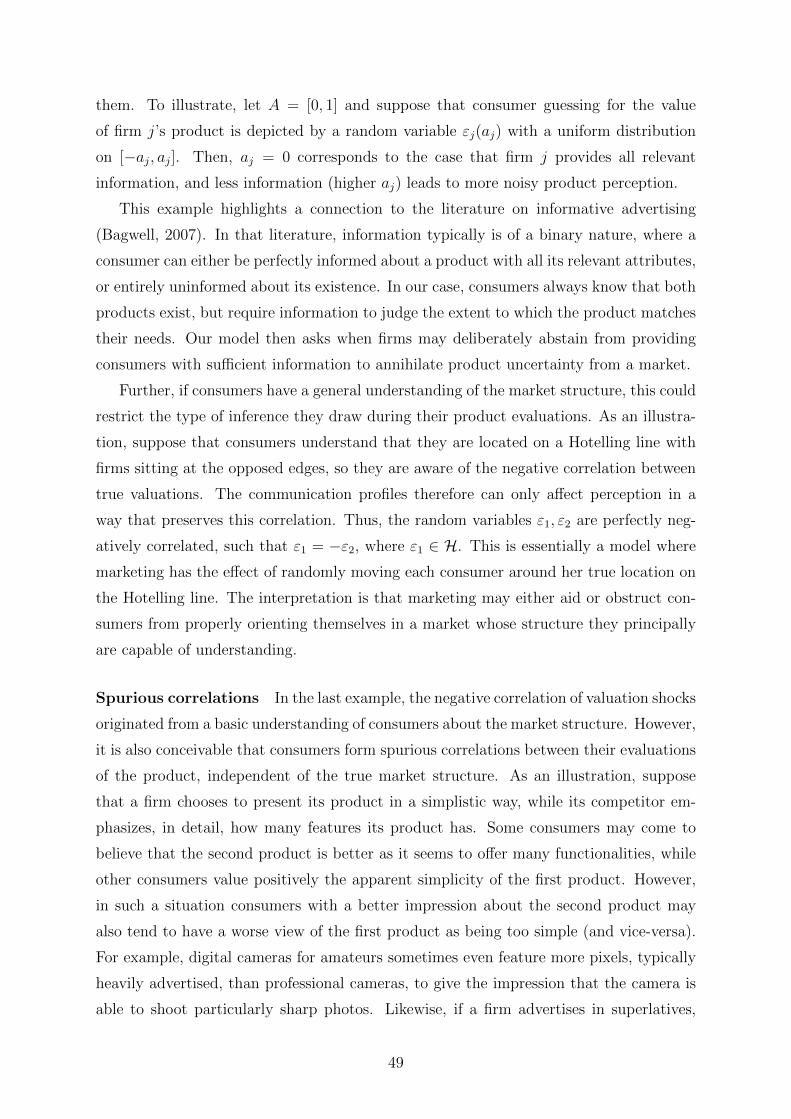
them. To illustrate, let A = [0, 1] and suppose that consumer guessing for the value

of firm j’s product is depicted by a random variable εj(aj) with a uniform distribution

on [−aj, aj]. Then, aj = 0 corresponds to the case that firm j provides all relevant

information, and less information (higher aj) leads to more noisy product perception.

This example highlights a connection to the literature on informative advertising

(Bagwell, 2007). In that literature, information typically is of a binary nature, where a

consumer can either be perfectly informed about a product with all its relevant attributes,

or entirely uninformed about its existence. In our case, consumers always know that both

products exist, but require information to judge the extent to which the product matches

their needs. Our model then asks when firms may deliberately abstain from providing

consumers with sufficient information to annihilate product uncertainty from a market.

Further, if consumers have a general understanding of the market structure, this could

restrict the type of inference they draw during their product evaluations. As an illustra-

tion, suppose that consumers understand that they are located on a Hotelling line with

firms sitting at the opposed edges, so they are aware of the negative correlation between

true valuations. The communication profiles therefore can only affect perception in a

way that preserves this correlation. Thus, the random variables ε1, ε2 are perfectly neg-

atively correlated, such that ε1 = −ε2, where ε1 ∈ H. This is essentially a model where

marketing has the effect of randomly moving each consumer around her true location on

the Hotelling line. The interpretation is that marketing may either aid or obstruct con-

sumers from properly orienting themselves in a market whose structure they principally

are capable of understanding.

Spurious correlations In the last example, the negative correlation of valuation shocks

originated from a basic understanding of consumers about the market structure. However,

it is also conceivable that consumers form spurious correlations between their evaluations

of the product, independent of the true market structure. As an illustration, suppose

that a firm chooses to present its product in a simplistic way, while its competitor em-

phasizes, in detail, how many features its product has. Some consumers may come to

believe that the second product is better as it seems to offer many functionalities, while

other consumers value positively the apparent simplicity of the first product. However,

in such a situation consumers with a better impression about the second product may

also tend to have a worse view of the first product as being too simple (and vice-versa).

For example, digital cameras for amateurs sometimes even feature more pixels, typically

heavily advertised, than professional cameras, to give the impression that the camera is

able to shoot particularly sharp photos. Likewise, if a firm advertises in superlatives,

49

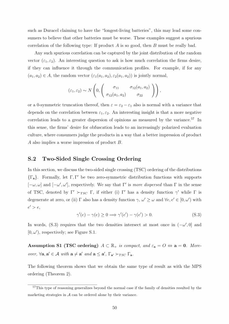
such as Duracel claiming to have the “longest-living batteries”, this may lead some con-

sumers to believe that other batteries must be worse. These examples suggest a spurious

correlation of the following type: If product A is so good, then B must be really bad.

Any such spurious correlation can be captured by the joint distribution of the random

vector (ε1, ε2). An interesting question to ask is how much correlation the firms desire,

if they can influence it through the communication profiles. For example, if for any

(a1, a2) ∈ A, the random vector (ε1(a1, a2), ε2(a1, a2)) is jointly normal,

(ε1, ε2) ∼ N

(0,

(σ11 σ12(a1, a2)

σ12(a1, a2) σ22

)),

or a 0-symmetric truncation thereof, then ε = ε2− ε1 also is normal with a variance that

depends on the correlation between ε1, ε2. An interesting insight is that a more negative

correlation leads to a greater dispersion of opinions as measured by the variance.57 In

this sense, the firms’ desire for obfuscation leads to an increasingly polarized evaluation

culture, where consumers judge the products in a way that a better impression of product

A also implies a worse impression of product B.

S.2 Two-Sided Single Crossing Ordering

In this section, we discuss the two-sided single crossing (TSC) ordering of the distributions

{Γa}. Formally, let Γ,Γ′ be two zero-symmetric distribution functions with supports

[−ω, ω] and [−ω′, ω′], respectively. We say that Γ′ is more dispersed than Γ in the sense

of TSC, denoted by Γ′ �TSC Γ, if either (i) Γ′ has a density function γ′ while Γ is

degenerate at zero, or (ii) Γ also has a density function γ, ω′ ≥ ω and ∀e, e′ ∈ [0, ω′) with

e′ > e,

γ′(e)− γ(e) ≥ 0 =⇒ γ′(e′)− γ(e′) > 0. (S.3)

In words, (S.3) requires that the two densities intersect at most once in (−ω′, 0] and

[0, ω′), respectively; see Figure S.1.

Assumption S1 (TSC ordering) A ⊂ R+ is compact, and εa = O ⇔ a = 0. More-

over, ∀a, a′ ∈ A with a 6= a′ and a ≤ a′, Γa′ �TSC Γa.

The following theorem shows that we obtain the same type of result as with the MPS

ordering (Theorem 2).

57This type of reasoning generalizes beyond the normal case if the family of densities resulted by the

marketing strategies in A can be ordered alone by their variance.

50

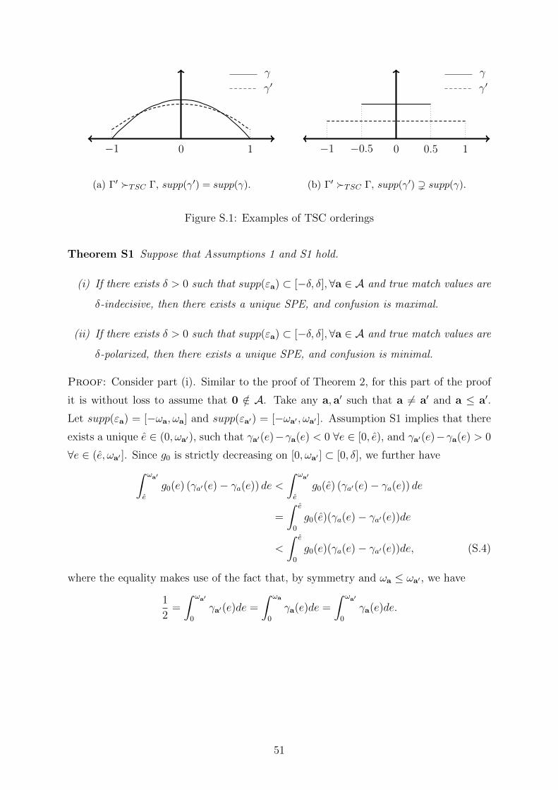
0−1 1

γ

γ′

(a) Γ′ �TSC Γ, supp(γ′) = supp(γ).

0−0.5 0.5−1 1

γ

γ′

(b) Γ′ �TSC Γ, supp(γ′) ) supp(γ).

Figure S.1: Examples of TSC orderings

Theorem S1 Suppose that Assumptions 1 and S1 hold.

(i) If there exists δ > 0 such that supp(εa) ⊂ [−δ, δ],∀a ∈ A and true match values are

δ-indecisive, then there exists a unique SPE, and confusion is maximal.

(ii) If there exists δ > 0 such that supp(εa) ⊂ [−δ, δ],∀a ∈ A and true match values are

δ-polarized, then there exists a unique SPE, and confusion is minimal.

Proof: Consider part (i). Similar to the proof of Theorem 2, for this part of the proof

it is without loss to assume that 0 /∈ A. Take any a, a′ such that a 6= a′ and a ≤ a′.

Let supp(εa) = [−ωa, ωa] and supp(εa′) = [−ωa′ , ωa′ ]. Assumption S1 implies that there

exists a unique e ∈ (0, ωa′), such that γa′(e)−γa(e) < 0 ∀e ∈ [0, e), and γa′(e)−γa(e) > 0

∀e ∈ (e, ωa′ ]. Since g0 is strictly decreasing on [0, ωa′ ] ⊂ [0, δ], we further have∫ ωa′

e

g0(e) (γa′(e)− γa(e)) de <∫ ωa′

e

g0(e) (γa′(e)− γa(e)) de

=

∫ e

0

g0(e)(γa(e)− γa′(e))de

<

∫ e

0

g0(e)(γa(e)− γa′(e))de, (S.4)

where the equality makes use of the fact that, by symmetry and ωa ≤ ωa′ , we have

1

2=

∫ ωa′

0

γa′(e)de =

∫ ωa

0

γa(e)de =

∫ ωa′

0

γa(e)de.

51

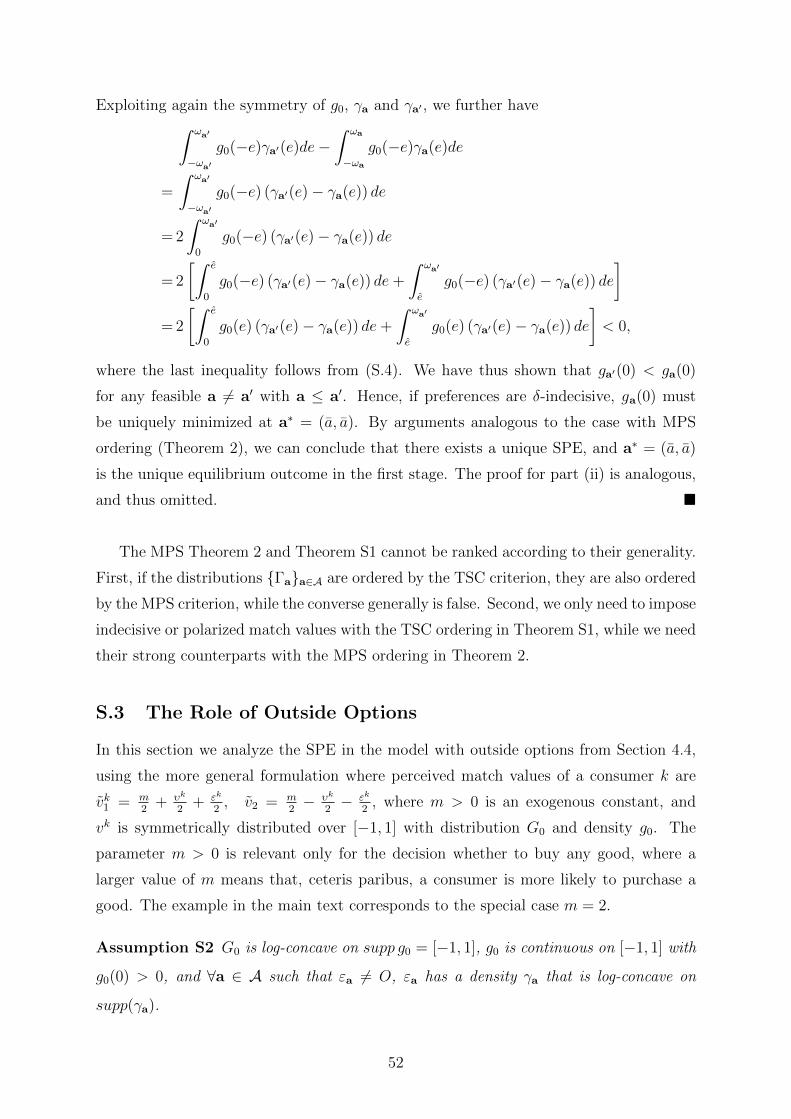
Exploiting again the symmetry of g0, γa and γa′ , we further have∫ ωa′

−ωa′

g0(−e)γa′(e)de−∫ ωa

−ωa

g0(−e)γa(e)de

=

∫ ωa′

−ωa′

g0(−e) (γa′(e)− γa(e)) de

= 2

∫ ωa′

0

g0(−e) (γa′(e)− γa(e)) de

= 2

[∫ e

0

g0(−e) (γa′(e)− γa(e)) de+

∫ ωa′

e

g0(−e) (γa′(e)− γa(e)) de

]= 2

[∫ e

0

g0(e) (γa′(e)− γa(e)) de+

∫ ωa′

e

g0(e) (γa′(e)− γa(e)) de

]< 0,

where the last inequality follows from (S.4). We have thus shown that ga′(0) < ga(0)

for any feasible a 6= a′ with a ≤ a′. Hence, if preferences are δ-indecisive, ga(0) must

be uniquely minimized at a∗ = (a, a). By arguments analogous to the case with MPS

ordering (Theorem 2), we can conclude that there exists a unique SPE, and a∗ = (a, a)

is the unique equilibrium outcome in the first stage. The proof for part (ii) is analogous,

and thus omitted. �

The MPS Theorem 2 and Theorem S1 cannot be ranked according to their generality.

First, if the distributions {Γa}a∈A are ordered by the TSC criterion, they are also ordered

by the MPS criterion, while the converse generally is false. Second, we only need to impose

indecisive or polarized match values with the TSC ordering in Theorem S1, while we need

their strong counterparts with the MPS ordering in Theorem 2.

S.3 The Role of Outside Options

In this section we analyze the SPE in the model with outside options from Section 4.4,

using the more general formulation where perceived match values of a consumer k are

vk1 = m2

+ υk

2+ εk

2, v2 = m

2− υk

2− εk

2, where m > 0 is an exogenous constant, and

vk is symmetrically distributed over [−1, 1] with distribution G0 and density g0. The

parameter m > 0 is relevant only for the decision whether to buy any good, where a

larger value of m means that, ceteris paribus, a consumer is more likely to purchase a

good. The example in the main text corresponds to the special case m = 2.

Assumption S2 G0 is log-concave on supp g0 = [−1, 1], g0 is continuous on [−1, 1] with

g0(0) > 0, and ∀a ∈ A such that εa 6= O, εa has a density γa that is log-concave on

supp(γa).

52

In the current setting, the distribution of vk coincides with the distribution of the true

match advantages. As a result, Assumption S2 implies Conditions (i)-(iii) of Proposition

1. These conditions assured the existence of a unique symmetric equilibrium in the pricing

stage of the game without outside option for any given communication profile a ∈ A, and

play a similar role here. We begin our analysis with a characterization of the symmetric

equilibria in the pricing stage.

Proposition S1 Suppose that Assumption S2 holds. In the above game with outside

option, there exists a unique symmetric pure-strategy equilibrium in the pricing stage,

and ∀a ∈ A both firms choose the price

p∗a =

1

2ga(0)if ga(0) > 1

m,

m2

if ga(0) ∈[

12m, 1m

],

pMa > m2

otherwise,

(S.5)

where pMa solves the monopoly problem maxp≥0 ΠMa (p) ≡ p (1−Ga(2p−m)) . The equi-

librium demand of each firm is strictly less than 1/2 if and only if ga(0) < 12m

.

All proofs are at the end of this section. The competition resulting from the presence

of sufficiently many perceptually indifferent consumers (ga(0) > 1/m) disciplines both

firms to choose an equilibrium price for which the outside option is non-binding for every

consumer.58 For lower values of ga(0), competition is less intense, yielding a strong

temptation to increase prices. As long as ga(0) ∈ [ 12m, 1m

], both firms settle exactly at

the price p = m/2 that just keeps every consumer in the market.59 By contrast, for

ga(0) < 12m

firms increase prices even though some consumers exit the market.

In essence, the pricing pattern identified by Proposition S1 determines what type of

communication strategies the firms choose in the first stage. Specifically, if ga(0) ≥ 1m

∀a ∈ A, the SPE identified by Theorems 1 and 2 apply given the respective assumptions

on g0. Further, if true preferences are strongly indecisive on supp g0 = [−1, 1], ga(0) ≥ 12m

∀a ∈ A and {Γa} verify an MPS order, maximal obfuscation is always an SPE outcome.60

Most importantly, Proposition S1 suggests that the firms may desire to confuse on a

massive scale so that they can then exploit some local monopoly power, even though

many consumers choose to exit.

58See Armstrong and Zhou (2019) for a similar result in a different setup.59Absent a binding outside option, both firms would increase their price above m/2.60The only difference to the case without outside option is that uniqueness of equilibrium may fail,

despite an MPS ordering. In particular, any a ∈ A inducing a value ga(0) ∈ [ 12m ,

1m ] is an SPE with

second-stage price p∗a = m/2.

53

To confirm this idea, we now analyze the tractable case where Γa follows a uniform

distribution with support [−ωa, ωa], ∀a ∈ A, and g0(0) > 1m

. The latter assumption

implies that without confusion the equilibrium price p∗0 = 12g0(0)

is such that the outside

option is non-binding for all consumers. In addition, we assume that m ≥ 2, which sim-

plifies the presentation of results. We first apply Proposition S1 to derive the equilibrium

price, firm demand and payoff as a function of consumer confusion ω given that confusion

is massive (ω ≥ 1).

Corollary S1 Let m ≥ 2 and suppose that Assumption S2 is satisfied. For any given

ω > 0, let Γω follow a uniform distribution with support [−ω, ω], and let pω denote the

symmetric equilibrium price in the pricing game given consumer confusion Γω. Likewise,

let dω and Πω denote the corresponding demand and payoff of each firm. Then pω, dω,Πω :

R++ → R are continuous functions of ω, and if confusion is massive (ω ≥ 1), we have

pω =

ω if ω ∈

[1, m

2

)m2

if ω ∈[m2,m]

ω+m4

if ω > m

, dω =

12

if ω ∈ [1,m]

ω+m4ω

if ω > m

,

and Πω = pωdω. If 1 ≤ ω ≤ m all consumers buy a product; if ω > m the fraction of

consumers leaving the market is L(ω) = ω−m2ω

> 0, which is strictly increasing in ω with

limω→∞ L(ω) = 1/2.

Corollary S1 shows that equilibrium prices and payoffs are increasing and unbounded in

the range of confusion ω, despite an increasing fraction of consumers who abstain from

acquiring any product.

We now ask how the intensity of confusion ω = ωa is determined by strategically

behaving firms that fully anticipate the profit schedule Πω resulting from the various

feasible confusion intensities. We impose a structure on the mapping a 7→ ωa that

is consistent with the MPS order Assumption 3: A ⊂ R+ is compact, 0 ∈ A, and

ω : A → R+ is such that ωa′ > ωa iff a′ ≥ a and a′ 6= a.61 Further, define a ≡ maxA > 0

and ω ≡ ωa as the maximally feasible confusion. Given this structure, we now show that

the SPE follow the same pattern as identified by Theorems 1-3 except that the chosen

communication strategies may lead to consumer exit from the market.

Consider first the case where ω ≤ 1, such that massive confusion is not feasible. If

preferences are indecisive on [−1, 1], then ga(0) = 12ωa

∫ ωa

−ωag0(e)de is strictly decreasing

61It is easily checked that the uniform distribution verifies the TSC order criterion (see Appendix S1).

A simple example is given by ω(a) = z(a1 +a2) where z is any strictly increasing function with z(0) = 0.

54

in the intensity of confusion ωa, and ga(0) ≥ 12ω∀a ∈ A. Because m ≥ 2 also assures

12ω> 1

m, it follows that ga(0) > 1

m∀a ∈ A, and Proposition S1 implies that p∗a = 1

2ga(0),

∀a ∈ A. This shows that with indecisive preferences and ω ≤ 1 (i) any SPE is such that

no consumer leaves the market, (ii) there cannot be an SPE without confusion (as in

Theorem 1), and (iii) maximal confusion is the unique SPE outcome in case of strongly

indecisive preferences (as in Theorem 2). If preferences are polarized on [−1, 1], then ga(0)

must be strictly increasing in the intensity of confusion ωa. Together with g0(0) > 1m

it

follows from Proposition S1 that p∗a = 12ga(0)

, ∀a ∈ A. Thus, (i) any SPE is such that

no consumer leaves the market, (ii) education always is an SPE outcome (as in Theorem

1), and education is the unique SPE outcome with strongly polarized preferences (as in

Theorem 2).

The following result allows for the possibility that massive confusion may arise. The

main point is that maximal confusion becomes the unique SPE outcome if confusion can

become massive enough, even though a substantial portion of consumers chooses not to

buy at all.

Proposition S2 Consider the above example where Γa follows a uniform distribution for

each a ∈ A. If G0 is indecisive on supp g0, then a unique SPE with maximal confusion

always exists, and a fraction max{ ω−m2ω

, 0} of consumers leaves the market. If G0 is

polarized on supp g0, then maximal confusion is an SPE outcome whenever ω ≥ m2

, and

the unique SPE whenever ω > m, in which case a fraction ω−m2ω∈ (0, 1

2) of consumers

leaves the market.

S.3.1 Proofs

Proof of Proposition S1 For any given Γa, the demand function of firm 1 is

Da(p1, p2) =

∫Pr(vk1 − p1 ≥ max{vk2 − p2, 0}

)dΓa

=

∫Pr (υ ≥ p1 − p2 − e, υ ≥ 2p1 −m− e) dΓa(e)

=

∫min {Pr (υ ≥ p1 − p2 − e) ,Pr (υ ≥ 2p1 −m− e)} dΓa(e)

=1−∫

max {G0 (p1 − p2 − e) , G0 (2p1 −m− e)} dΓa(e).

Recall that, for all x ∈ R,

Ga(x) =

∫G0(x− e)dΓa(e), and ga(x) =

∫g0(x− e)dΓa(e).

55

Thus, for all p ≥ 0, we have

Da(p, p) =

12

if p ≤ m2,

1−Ga(2p−m) if p > m2.

(A.6)

Let Πa1(p1, p2) = p1Da(p1, p2). For every p2 > 0, the function Πa

1 is differentiable in p1

almost everywhere. In particular, if p1 < m− p2, such that Da(p1, p2) = 1−Ga(p1− p2),

we have

∂Πa1(p1, p2)

∂p1

= 1−Ga(p1 − p2)− p1ga(p1 − p2),

which is also the left derivative of Πa1(p1, p2) at p1 = m − p2. Similarly, if p1 > m − p2,

such that Da(p1, p2) = 1−Ga(2p1 −m), we have

∂Πa1(p1, p2)

∂p1

= 1−Ga(2p1 −m)− 2p1ga(2p1 −m),

which is also the right derivative of Πa1(p1, p2) at p1 = m− p2.

Since log-concavity is preserved under convolution, the function Ga is log-concave on

its support supp(ga). In addition, since Ga is a distribution function, its log-concavity

also holds on [0,+∞). Hence, for all p2 > 0 and a ∈ A, the demand function Da(p1, p2)

must be log-concave in p1 on both [0,m − p2] and [m − p2,+∞). Note that we are

not claiming that Da(p1, p2) is log-concave in p1 on the entire interval [0,+∞). In what

follows, we will show that although the global log-concavity of the demand function is not

assured, Assumption S2 is still sufficient to guarantee the existence of a unique symmetric

equilibrium in every subgame of the pricing stage.

First, suppose that ga(0) > 1m

. Suppose also that firm 2 is choosing p2 = 12ga(0)

< m2

.

Then, for any p1 ≤ m2

the whole market is guaranteed to be covered (i.e., every consumer

will buy from one of the firms). In addition, since

∂Πa1(p1, p2)

∂p1

∣∣∣∣∣p1=p2= 1

2ga(0)<m

2

= 1−Ga(0)− 1

2ga(0)· ga(0) = 0,

and the function Πa1

(p1,

12ga(0)

)is strictly quasi-concave in p1 on

[0,m− 1

2ga(0)

], and

ga(0) > 1m

implies that p1 = 12ga(0)

maximizes the function Πa1

(p1,

12ga(0)

)over the range[

0,m− 12ga(0)

]. We now argue that, in addition,

Πa1

(p1,

1

2ga(0)

)< Πa

1

(1

2ga(0),

1

2ga(0)

)∀p1 > m− 1

2ga(0).

To see this, note that if p1 > m − 12ga(0)

, then some consumers choose their outside

options even though they would prefer firm 1 over firm 2. Therefore, a deviation to

56

p1 > m − 12ga(0)

cannot be more profitable than it would have been in the case without

outside option. But then, as we have shown in Lemma 1 and Proposition 1, in the

absence of the outside option, choosing p1 = 12ga(0)

actually uniquely maximizes firm 1’s

expected profits over [0,+∞) given that its competitor plays p2 = 12ga(0)

. This implies

that deviating to p1 > m− 12ga(0)

cannot be profitable either in the presence of the outside

option. Therefore, p1 = 12ga(0)

must be a global maximum of the function Πa1

(p1,

12ga(0)

),

and (p1, p2) =(

12ga(0)

, 12ga(0)

)indeed constitutes an equilibrium in the pricing subagme.

It is easy to see that this is the only symmetric equilibrium with a price strictly less thanm2

. In addition, since

∂ΠMa (p)

∂p

∣∣∣∣∣p=m

2

=1

2−m · ga(0) <

1

2− 1 < 0

and ΠMa (p) is strictly quasi-concave, even a monopoly firm would not choose a price

p ≥ m2

. Hence, when ga(0) > 1m

, there cannot be any symmetric equilibrium in which

both firms choose a price larger than m2

. As a result, (p1, p2) =(

12ga(0)

, 12ga(0)

)is the

unique symmetric pure-strategy equilibrium when ga(0) > 1m

.

Next, consider the case ga(0) ∈ [ 12m, 1m

]. Taking p2 = m2

as given, we will show that

p1 = m2

is a best response for firm 1. As mentioned, the profit function Π1(p1, p2) is

differentiable in p1 on R++\{m − p2} and semi-differentiable at the point p1 = m − p2.

In particular, we have

∂−Πa1(p1, p2)

∂p1

∣∣∣∣∣p1=p2=m

2

= 1−Ga(0)− m

2· ga(0) =

1

2− m

2· ga(0) ≥ 0,

and

∂+Πa1(p1, p2)

∂p1

∣∣∣∣∣p1=p2=m

2

= 1−Ga(0)−mga(0) =1

2−m · ga(0) ≤ 0.

Since Πa1

(p1,

m2

)is strictly quasi-concave on both

[0, m

2

]and [m

2,+∞), the above in-

equalities imply that p1 = m2

is a maximum of Πa1

(p1,

12

)on each of these two inter-

vals. This shows that p1 = m2

is a global maximum of Πa1

(p1,

m2

)on [0,+∞). Hence,

if ga(0) ∈ [ 12m, 1m

], the game in the pricing stage admits a symmetric equilibrium with

p1 = p2 = m2

. Further, as ga(0) ≤ 1m

a symmetric equilibrium with p1 = p2 <m2

cannot

exist. To see this, note that a symmetric equilibrium with p1 = p2 <m2

involves full

market coverage (as p1 < m− p2), and must be a solution to the first order condition

1−Ga(0)− p1ga(0) = 0.

57

Thus p1 = 12ga(0)

, where the condition p1 < m2

therefore is equivalent to ga(0) > 1m

,

contradiction.

In addition, because

∂ΠMa (p)

∂p

∣∣∣∣∣p=m

2

=1

2−m · ga(0) ≤ 1

2− 1

2= 0

and ΠMa (p) is strictly quasi-concave, even a monopoly firm would not choose a price

strictly higher than m2

. Hence, no symmetric equilibrium with p1 = p2 >m2

can exist

either. In sum, this shows that (p1, p2) =(m2, m

2

)is the unique symmetric pure-strategy

equilibrium when ga(0) ∈[

12m, 1m

].

Finally, suppose that ga(0) < 12m

. Observe that in this case, we have pMa > m2

, because

∂ΠMa (p)

∂p

∣∣∣∣∣p=m

2

=1

2−m · ga(0) > 0

and ΠMa (p) is strictly quasi-concave on [0,+∞). Now suppose that firm 2 plays p2 = pMa ,

and consider firm 1’s profit function Π1(p1, pMa ). Given the formula of the demand function

and pMa > m− pMa , we have

Πa1(pMa , p

Ma ) = ΠM

a (pMa ) > ΠMa (p1) ≥ Πa

1(p1, pMa ) ∀p1 ∈ [0,+∞)\{pMa },

which further implies that p1 = pMa is the unique best response for firm 1. Hence,

(p1, p2) =(pMa , p

Ma

)indeed constitutes an equilibrium in the pricing subgame where

ga(0) < 12m

. Moreover, given 12ga(0)

> m2

, there cannot exist a symmetric equilibrium with

p1 = p2 <m2

. Since

∂−Πa1(p1, p2)

∂p1

∣∣∣∣∣p1=p2=m

2

>∂+Πa

1(p1, p2)

∂p1

∣∣∣∣∣p1=p2=m

2

=1

2−m · ga(0) > 0,

p1 = p2 = m2

does not constitute an equilibrium either. In conclusion, (p1, p2) =(pMa , p

Ma

)is the unique symmetric pure-strategy equilibrium when ga(0) < 1

2m.

Taken together, the above derivations prove that the equilibrium price p∗a is deter-

mined by (S.5). Further, (A.6) implies that market shares are below 1/2 iff ga(0) < 12m

,

completing the proof. �

Proof of Corollary S1 Let gω denote the density of the perceived match advantages

given that the perception errors ε follow the uniform distribution Γω. It is easily checked

that for any ω > 0, the density γω is log-concave on its support. Thus, Assumption 4.4

is satisfied, and Proposition S1 applies to the case of uniformly distributed perception

58

errors. Specifically, the equilibrium price is determined by (S.5), where we replace p∗a by

pω and ga(0) by gω(0). For any given ω > 0, we have gω(0) = 12ω

∫ ω−ω g0(e)de. Next, note

that gω(0) = 12ω

∫ 1

−1g0(e)de = 1

2ωwhenever ω ≥ 1, which we assume in the following.

Given that ω ≥ 1, the condition gω(0) > 1m

is equivalent to ω < m2

. Thus, for ω ∈ [1, m2

),

we must have gω(0) = 12ω

> 1m

, and hence pω = 12gω(0)

= ω by (S.5). Next, given that

ω ≥ 1, the condition gω(0) ≥ 12m

is equivalent to ω ≤ m. Thus, for ω ∈ [m2,m] also

gω(0) ∈ [ 12m, 1m

], and thus pω = m2

for ω ∈ [m2,m] by (S.5). Finally, gω(0) < 1

2miff ω > m,

in which case (S.5) implies that pω is given by the monopoly price pMω . We now show

that if ω > m, then pω = pMω = ω+m4

, independent of the shape of g0. If pω denotes

the solution of this monopoly problem, then pω must be determined by the first order

condition ∂ΠMω (pω)∂p

= 0, which can be simplified to

ω − 1

2

∫ 2pω−m+ω

2pω−m−ωG0(s)ds− p

∫ 2pω−m+ω

2pω−m−ωg0(s)ds = 0 (S.6)

To calculate the value of pω we need to evaluate the two integrals in the previous expres-

sions. By Proposition S1, we know that pω >m2

, which implies that 2pω −m+ ω > 1 for

the upper bounds of the two integrals (recalling that ω ≥ 1). We now conjecture (and ex

post verify) that 2pω−m−ω < −1. Recalling that supp g0 = [−1, 1] and∫ 1

−1G0(s)ds = 1

as a consequence of symmetry, (S.6) evaluates to pω = ω+m4

given the presumption that

2pω −m−ω < −1. It now is easily verified that the last inequality indeed is satisfied for

pω = ω+m4

, confirming that pMω = ω+m4

must be the monopoly price. In sum, these steps

show that pω must be as stated by Corollary S1. Continuity of pω in ω then is obvious

for ω ∈ [1,∞). As the equilibrium price pω is determined by (S.5), it follows from (S.5)

and the previous result that pω is continuous on the entire range ω ∈ (0,∞) whenever

gω(0) is continuous in ω on this range. As gω(0) = 12ω

∫ ω−ω g0(e)de for any ω > 0, the last

property is obviously verified.

Turning to equilibrium demand, the proof of Proposition S1 shows that as long as

1 ≤ ω ≤ m (i.e., gω(0) ≥ 12m

) the equilibrium price is such that the outside option is not

binding for (almost) all consumers, meaning that dω = 1/2 for ω ∈ [1,m]. If ω > m, the

equilibrium price is given by pMω = ω+m4

, and dω = 1−Gω(2pMω −m), which evaluates to

dω = ω+m4ω

. The expression for equilibrium profits Πω = pωdω then follows immediately.

Continuity of dω and of Πω = pωdω in ω follow from the continuity of pω. Finally, the

claims about L(ω) follows from L(ω) = 1− 2dω. �

Proof of Proposition S2 Suppose that preferences are indecisive on [−1, 1]. If ω ≤ m,

the existence of a unique SPE with maximal confusion immediately follows from Theorem

S1. If ω > m, the same result holds because it is shown in Corollary S1 that Πω is

59

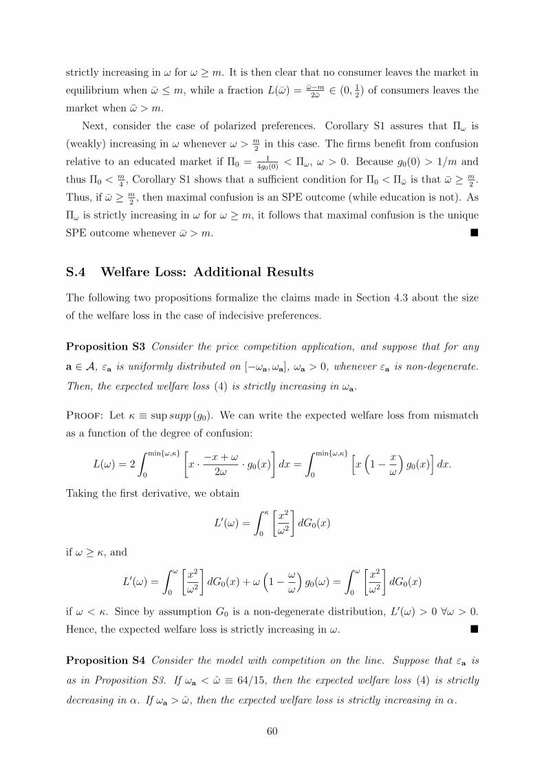
strictly increasing in ω for ω ≥ m. It is then clear that no consumer leaves the market in

equilibrium when ω ≤ m, while a fraction L(ω) = ω−m2ω∈ (0, 1

2) of consumers leaves the

market when ω > m.

Next, consider the case of polarized preferences. Corollary S1 assures that Πω is

(weakly) increasing in ω whenever ω > m2

in this case. The firms benefit from confusion

relative to an educated market if Π0 = 14g0(0)

< Πω, ω > 0. Because g0(0) > 1/m and

thus Π0 <m4

, Corollary S1 shows that a sufficient condition for Π0 < Πω is that ω ≥ m2

.

Thus, if ω ≥ m2

, then maximal confusion is an SPE outcome (while education is not). As

Πω is strictly increasing in ω for ω ≥ m, it follows that maximal confusion is the unique

SPE outcome whenever ω > m. �

S.4 Welfare Loss: Additional Results

The following two propositions formalize the claims made in Section 4.3 about the size

of the welfare loss in the case of indecisive preferences.

Proposition S3 Consider the price competition application, and suppose that for any

a ∈ A, εa is uniformly distributed on [−ωa, ωa], ωa > 0, whenever εa is non-degenerate.

Then, the expected welfare loss (4) is strictly increasing in ωa.

Proof: Let κ ≡ sup supp (g0). We can write the expected welfare loss from mismatch

as a function of the degree of confusion:

L(ω) = 2

∫ min{ω,κ}

0

[x · −x+ ω

2ω· g0(x)

]dx =

∫ min{ω,κ}

0

[x(

1− x

ω

)g0(x)

]dx.

Taking the first derivative, we obtain

L′(ω) =

∫ κ

0

[x2

ω2

]dG0(x)

if ω ≥ κ, and

L′(ω) =

∫ ω

0

[x2

ω2

]dG0(x) + ω

(1− ω

ω

)g0(ω) =

∫ ω

0

[x2

ω2

]dG0(x)

if ω < κ. Since by assumption G0 is a non-degenerate distribution, L′(ω) > 0 ∀ω > 0.

Hence, the expected welfare loss is strictly increasing in ω. �

Proposition S4 Consider the model with competition on the line. Suppose that εa is

as in Proposition S3. If ωa < ω ≡ 64/15, then the expected welfare loss (4) is strictly

decreasing in α. If ωa > ω, then the expected welfare loss is strictly increasing in α.

60

Proof: Since G0(x) = H(x4λ

)∀x ∈ R, the density function of G0, which we denote as

g0, is given by

g0(x) =1

4λh( x

4λ

)=

1

4λ·(α(x4λ

)2+ 1

2λ− αλ2

3

)if x ∈ [−4λ2, 4λ2],

0 otherwise.

The welfare loss can now be written as a function of α:

L(α) =

∫ min{ω,4λ2}

0

[x(

1− x

ω

)· 1

4λ· h( x

4λ

)]dx

=1

4λ

∫ min{ω,4λ2}

0

[x(

1− x

ω

)(α( x

4λ

)2

+1

2λ− αλ2

3

)]dx.

Taking derivative with respect to α, we have

L′(α) =1

4λ

∫ min{ω,4λ2}

0

[x(

1− x

ω

)(( x4λ

)2

− λ2

3

)]dx.

First, suppose that ω ≤ 4λ2. In this case, we obtain

L′(α) =1

4λ

∫ ω

0

[x(

1− x

ω

)(( x4λ

)2

− λ2

3

)]dx

=1

4λ

[∫ ω

0

(x3

16λ2− λ2x

3

)dx−

∫ ω

0

(x4

16λ2ω− λ2x2

3ω

)dx

]=

1

4λ

[(x4

64λ2− λ2x2

6

) ∣∣∣∣∣ω

0

−(

x5

80λ2ω− λ2x3

9ω

) ∣∣∣∣∣ω

0

]

=1

4λ

[ω4

64λ2− ω4

80λ2− λ2ω2

6+λ2ω2

9

].

Hence, provided that ω ∈ (0, 4λ2], we further have

L′(α) < 0 ⇐⇒(

1

64λ2− 1

80λ2

)ω2 <

λ2

6− λ2

9⇐⇒ ω <

4√

10

3λ2.

Since 4√

10/3 ≈ 4.22 > 4, it follows that L′(α) < 0 whenever ω ≤ 4λ2.

Next, consider the case where ω > 4λ2. Expanding the equation L′(α) again, we have

L′(α) =1

4λ

∫ 4λ2

0

[x(

1− x

ω

)(( x4λ

)2

− λ2

3

)]dx

=1

4λ

( x4

64λ2− λ2x2

6

) ∣∣∣∣∣4λ2

0

−(

x5

80λ2ω− λ2x3

9ω

) ∣∣∣∣∣4λ2

0

=

1

4λ

[(44λ8

64λ2− 42λ6

6

)− 1

ω

(45λ10

80λ2− 43λ8

9

)]= 4λ5

[(16

64− 1

6

)− λ2

ω

(64

80− 4

9

)].

61

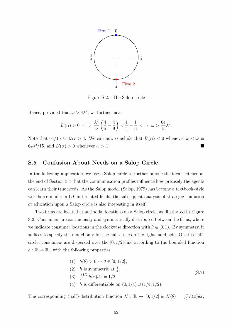
34

14

0

12

Firm 2

Firm 1

Figure S.2: The Salop circle

Hence, provided that ω > 4λ2, we further have

L′(α) > 0 ⇐⇒ λ2

ω

(4

5− 4

9

)<

1

4− 1

6⇐⇒ ω >

64

15λ2.

Note that 64/15 ≈ 4.27 > 4. We can now conclude that L′(α) < 0 whenever ω < ω ≡64λ2/15, and L′(α) > 0 whenever ω > ω. �

S.5 Confusion About Needs on a Salop Circle

In the following application, we use a Salop circle to further pursue the idea sketched at

the end of Section 3.4 that the communication profiles influence how precisely the agents

can learn their true needs. As the Salop model (Salop, 1979) has become a textbook-style

workhorse model in IO and related fields, the subsequent analysis of strategic confusion

or education upon a Salop circle is also interesting in itself.

Two firms are located at antipodal locations on a Salop circle, as illustrated in Figure

S.2. Consumers are continuously and symmetrically distributed between the firms, where

we indicate consumer locations in the clockwise direction with θ ∈ [0, 1). By symmetry, it

suffices to specify the model only for the half-circle on the right-hand side. On this half-

circle, consumers are dispersed over the [0, 1/2]-line according to the bounded function

h : R→ R+ with the following properties

(1) h(θ) > 0⇔ θ ∈ [0, 1/2] ,

(2) h is symmetric at 14.

(3)∫ 1/2

0h(x)dx = 1/2,

(4) h is differentiable on (0, 1/4) ∪ (1/4, 1/2),

(S.7)

The corresponding (half)-distribution function H : R → [0, 1/2] is H(θ) =∫ θ

0h(x)dx,

62

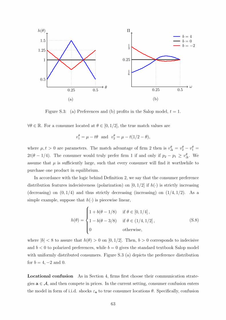
θ

1

0.5

1.25

1.5

0.50.25

h(θ)

(a)

ω0.5

0.25

16

13

Π

0.25

b = 4b = 0b = −2

(b)

Figure S.3: (a) Preferences and (b) profits in the Salop model, t = 1.

∀θ ∈ R. For a consumer located at θ ∈ [0, 1/2], the true match values are

vθ1 = µ− tθ and vθ2 = µ− t(1/2− θ),

where µ, t > 0 are parameters. The match advantage of firm 2 then is vθ∆ = vθ2 − vθ1 =

2t(θ − 1/4). The consumer would truly prefer firm 1 if and only if p2 − p1 ≥ vθ∆. We

assume that µ is sufficiently large, such that every consumer will find it worthwhile to

purchase one product in equilibrium.

In accordance with the logic behind Definition 2, we say that the consumer preference

distribution features indecisiveness (polarization) on [0, 1/2] if h(·) is strictly increasing

(decreasing) on (0, 1/4) and thus strictly decreasing (increasing) on (1/4, 1/2). As a

simple example, suppose that h(·) is piecewise linear,

h(θ) =

1 + b(θ − 1/8) if θ ∈ [0, 1/4] ,

1− b(θ − 3/8) if θ ∈ (1/4, 1/2] ,

0 otherwise,

(S.8)

where |b| < 8 to assure that h(θ) > 0 on [0, 1/2]. Then, b > 0 corresponds to indecisive

and b < 0 to polarized preferences, while b = 0 gives the standard textbook Salop model

with uniformly distributed consumers. Figure S.3 (a) depicts the preference distribution

for b = 4,−2 and 0.

Locational confusion As in Section 4, firms first choose their communication strate-

gies a ∈ A, and then compete in prices. In the current setting, consumer confusion enters

the model in form of i.i.d. shocks εa to true consumer locations θ. Specifically, confusion

63

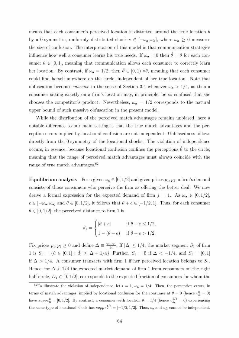
means that each consumer’s perceived location is distorted around the true location θ

by a 0-symmetric, uniformly distributed shock e ∈ [−ωa, ωa], where ωa ≥ 0 measures

the size of confusion. The interpretation of this model is that communication strategies

influence how well a consumer learns his true needs. If ωa = 0 then θ = θ for each con-

sumer θ ∈ [0, 1], meaning that communication allows each consumer to correctly learn

her location. By contrast, if ωa = 1/2, then θ ∈ [0, 1) ∀θ, meaning that each consumer

could find herself anywhere on the circle, independent of her true location. Note that

obfuscation becomes massive in the sense of Section 3.4 whenever ωa > 1/4, as then a

consumer sitting exactly on a firm’s location may, in principle, be so confused that she

chooses the competitor’s product. Nevertheless, ωa = 1/2 corresponds to the natural

upper bound of such massive obfuscation in the present model.

While the distribution of the perceived match advantages remains unbiased, here a

notable difference to our main setting is that the true match advantages and the per-

ception errors implied by locational confusion are not independent. Unbiasedness follows

directly from the 0-symmetry of the locational shocks. The violation of independence

occurs, in essence, because locational confusion confines the perceptions θ to the circle,

meaning that the range of perceived match advantages must always coincide with the

range of true match advantages.62

Equilibrium analysis For a given ωa ∈ [0, 1/2] and given prices p1, p2, a firm’s demand

consists of those consumers who perceive the firm as offering the better deal. We now

derive a formal expression for the expected demand of firm j = 1. As ωa ∈ [0, 1/2],

e ∈ [−ωa, ωa] and θ ∈ [0, 1/2], it follows that θ + e ∈ [−1/2, 1]. Thus, for each consumer

θ ∈ [0, 1/2], the perceived distance to firm 1 is

d1 =

|θ + e| if θ + e ≤ 1/2,

1− (θ + e) if θ + e > 1/2.

Fix prices p1, p2 ≥ 0 and define ∆ ≡ p2−p1

2t. If |∆| ≤ 1/4, the market segment S1 of firm

1 is S1 = {θ ∈ [0, 1] : d1 ≤ ∆ + 1/4}. Further, S1 = ∅ if ∆ < −1/4, and S1 = [0, 1]

if ∆ > 1/4. A consumer transacts with firm 1 if her perceived location belongs to S1.

Hence, for ∆ < 1/4 the expected market demand of firm 1 from consumers on the right

half-circle, D1 ∈ [0, 1/2], corresponds to the expected fraction of consumers for whom the

62To illustrate the violation of independence, let t = 1, ωa = 1/4. Then, the perception errors, in

terms of match advantages, implied by locational confusion for the consumer at θ = 0 (hence v0∆ = 0)

have supp ε0a = [0, 1/2]. By contrast, a consumer with location θ = 1/4 (hence v

1/4∆ = 0) experiencing

the same type of locational shock has supp ε1/4a = [−1/2, 1/2]. Thus, εa and v∆ cannot be independent.

64

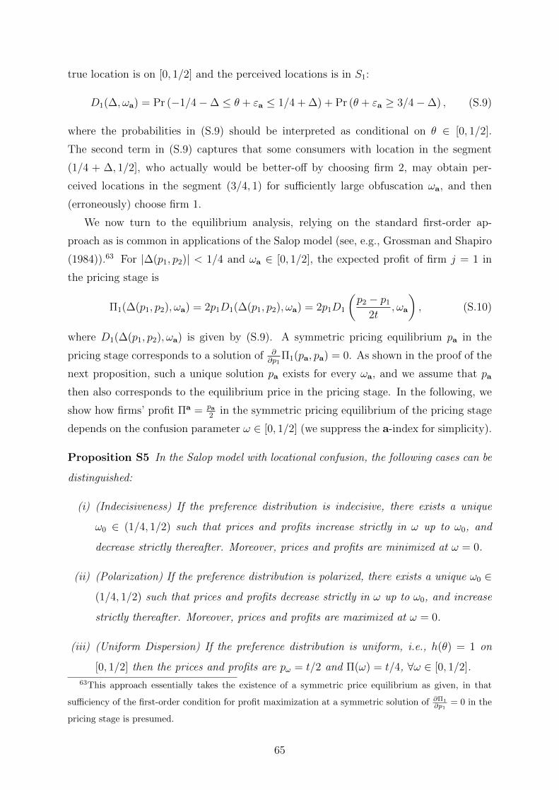
true location is on [0, 1/2] and the perceived locations is in S1:

D1(∆, ωa) = Pr (−1/4−∆ ≤ θ + εa ≤ 1/4 + ∆) + Pr (θ + εa ≥ 3/4−∆) , (S.9)

where the probabilities in (S.9) should be interpreted as conditional on θ ∈ [0, 1/2].

The second term in (S.9) captures that some consumers with location in the segment

(1/4 + ∆, 1/2], who actually would be better-off by choosing firm 2, may obtain per-

ceived locations in the segment (3/4, 1) for sufficiently large obfuscation ωa, and then

(erroneously) choose firm 1.

We now turn to the equilibrium analysis, relying on the standard first-order ap-

proach as is common in applications of the Salop model (see, e.g., Grossman and Shapiro

(1984)).63 For |∆(p1, p2)| < 1/4 and ωa ∈ [0, 1/2], the expected profit of firm j = 1 in

the pricing stage is

Π1(∆(p1, p2), ωa) = 2p1D1(∆(p1, p2), ωa) = 2p1D1

(p2 − p1

2t, ωa

), (S.10)

where D1(∆(p1, p2), ωa) is given by (S.9). A symmetric pricing equilibrium pa in the

pricing stage corresponds to a solution of ∂∂p1

Π1(pa, pa) = 0. As shown in the proof of the

next proposition, such a unique solution pa exists for every ωa, and we assume that pa

then also corresponds to the equilibrium price in the pricing stage. In the following, we

show how firms’ profit Πa = pa2

in the symmetric pricing equilibrium of the pricing stage

depends on the confusion parameter ω ∈ [0, 1/2] (we suppress the a-index for simplicity).

Proposition S5 In the Salop model with locational confusion, the following cases can be

distinguished:

(i) (Indecisiveness) If the preference distribution is indecisive, there exists a unique

ω0 ∈ (1/4, 1/2) such that prices and profits increase strictly in ω up to ω0, and

decrease strictly thereafter. Moreover, prices and profits are minimized at ω = 0.

(ii) (Polarization) If the preference distribution is polarized, there exists a unique ω0 ∈

(1/4, 1/2) such that prices and profits decrease strictly in ω up to ω0, and increase

strictly thereafter. Moreover, prices and profits are maximized at ω = 0.

(iii) (Uniform Dispersion) If the preference distribution is uniform, i.e., h(θ) = 1 on

[0, 1/2] then the prices and profits are pω = t/2 and Π(ω) = t/4, ∀ω ∈ [0, 1/2].

63This approach essentially takes the existence of a symmetric price equilibrium as given, in that

sufficiency of the first-order condition for profit maximization at a symmetric solution of ∂Π1

∂p1= 0 in the

pricing stage is presumed.

65

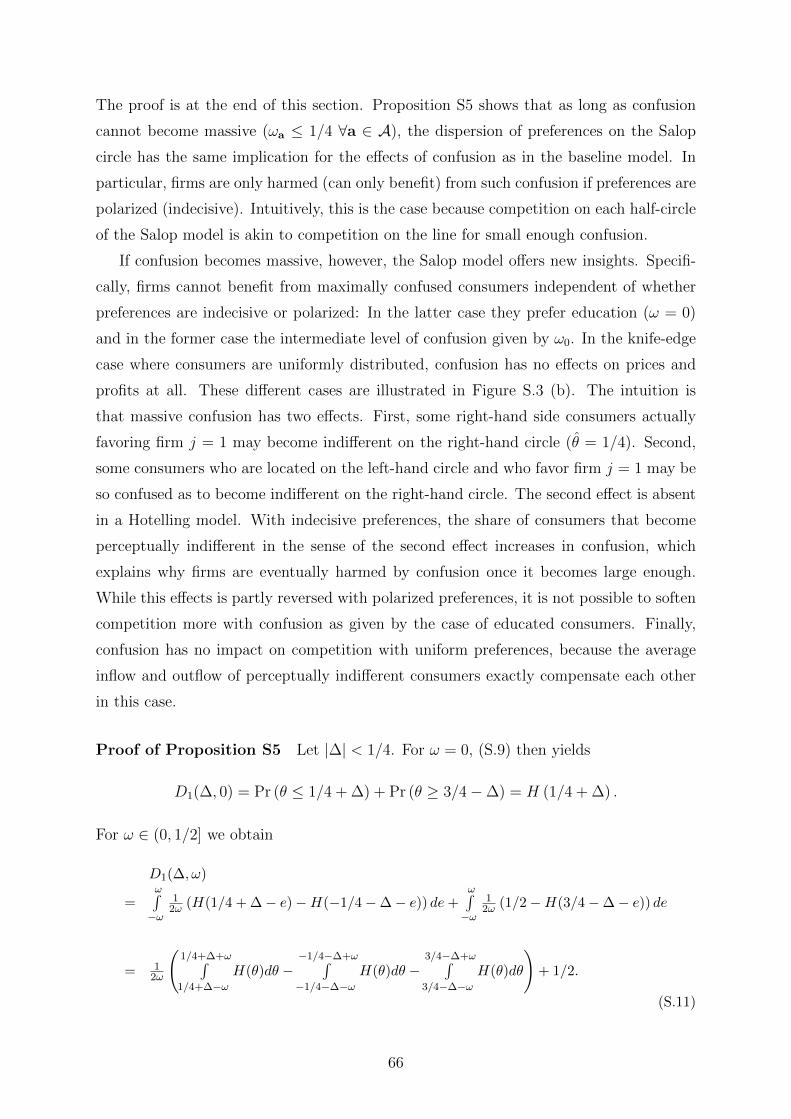
The proof is at the end of this section. Proposition S5 shows that as long as confusion

cannot become massive (ωa ≤ 1/4 ∀a ∈ A), the dispersion of preferences on the Salop

circle has the same implication for the effects of confusion as in the baseline model. In

particular, firms are only harmed (can only benefit) from such confusion if preferences are

polarized (indecisive). Intuitively, this is the case because competition on each half-circle

of the Salop model is akin to competition on the line for small enough confusion.

If confusion becomes massive, however, the Salop model offers new insights. Specifi-

cally, firms cannot benefit from maximally confused consumers independent of whether

preferences are indecisive or polarized: In the latter case they prefer education (ω = 0)

and in the former case the intermediate level of confusion given by ω0. In the knife-edge

case where consumers are uniformly distributed, confusion has no effects on prices and

profits at all. These different cases are illustrated in Figure S.3 (b). The intuition is

that massive confusion has two effects. First, some right-hand side consumers actually

favoring firm j = 1 may become indifferent on the right-hand circle (θ = 1/4). Second,

some consumers who are located on the left-hand circle and who favor firm j = 1 may be

so confused as to become indifferent on the right-hand circle. The second effect is absent

in a Hotelling model. With indecisive preferences, the share of consumers that become

perceptually indifferent in the sense of the second effect increases in confusion, which

explains why firms are eventually harmed by confusion once it becomes large enough.

While this effects is partly reversed with polarized preferences, it is not possible to soften

competition more with confusion as given by the case of educated consumers. Finally,

confusion has no impact on competition with uniform preferences, because the average

inflow and outflow of perceptually indifferent consumers exactly compensate each other

in this case.

Proof of Proposition S5 Let |∆| < 1/4. For ω = 0, (S.9) then yields

D1(∆, 0) = Pr (θ ≤ 1/4 + ∆) + Pr (θ ≥ 3/4−∆) = H (1/4 + ∆) .

For ω ∈ (0, 1/2] we obtain

D1(∆, ω)

=ω∫−ω

12ω (H(1/4 + ∆− e)−H(−1/4−∆− e)) de+

ω∫−ω

12ω (1/2−H(3/4−∆− e)) de

= 12ω

(1/4+∆+ω∫1/4+∆−ω

H(θ)dθ −−1/4−∆+ω∫−1/4−∆−ω

H(θ)dθ −3/4−∆+ω∫3/4−∆−ω

H(θ)dθ

)+ 1/2.

(S.11)

66

Then, (S.11) implies

∂D1(∆, ω)

∂∆=H(1/4 + ∆ + ω)−H(1/4 + ∆− ω)

2ω+H(−1/4−∆ + ω)−H(−1/4−∆− ω)

2ω

+H(3/4−∆ + ω)−H(3/4−∆− ω)

2ω. (S.12)

Using (S.12) and p2 = p1 = pω in the first-order condition then yields

pω =t/2

∂∂∆D1(0, ω)

(S.13)

as the unique solution. Then, the corresponding equilibrium profit Π(ω) ≡ pω/2 satisfies

signΠ′(ω) = sign∂pω∂ω

= −signZ(ω), Z(ω) ≡ ∂2D1(0, ω)

∂∆∂ω. (S.14)

Let ω ∈ (0, 1/4). Noting that h(θ) = 0 whenever θ /∈ [0, 1/2], we obtain from (S.12)

Z(ω) =2ωh(1/4 + ω)− (H(1/4 + ω)−H(1/4− ω))

2ω2.

The symmetry of h at θ = 1/4 implies

H (1/4 + ω)−H (1/4− ω) = 2H (1/4 + ω)− 1/2. (S.15)

Using this and H(1/4) = 1/4 in (S.15), we have

Z(ω) ≥ 0 ⇔ h (1/4 + ω)ω ≥ H (1/4 + ω)− 1/4 =

1/4+ω∫1/4

h(θ)dθ. (S.16)

Therefore we can establish the claims in (i), (ii) and (iii) for the case where ω ∈ (0, 1/4).

(i)1/4+ω∫1/4

h(θ)dθ >1/4+ω∫1/4

h(1/4 + ω)dθ = h(1/4 +ω)ω, thus Z(ω) < 0 by (S.16). Hence

prices and profits increase in obfuscation by (S.14) for ω ∈ (0, 1/4).

(ii)1/4+ω∫1/4

h(θ)dθ <1/4+ω∫1/4

h(1/4 + ω)dθ = h(1/4+ω)ω, thus Z(ω) > 0 by (S.16). Hence

prices and profits decrease in obfuscation by (S.14) for ω ∈ (0, 1/4).

(iii)1/4+ω∫1/4

h(θ)dθ = 1/4 +ω− 1/4 = ω, and h(

14

+ ω)ω = ω, thus Z(ω) = 0 by (S.16).

Hence obfuscation has no effects on prices and profits by (S.14) for ω ∈ (0, 1/4).

Next, suppose that ω ∈ (1/4, 1/2].64 Then, (S.12) gives

Z(ω) =ω (h(ω − 1/4) + h(3/4− ω))− (1 +H(ω − 1/4)−H(3/4− ω))

2ω2. (S.17)

64The case ω = 1/4 is not problematic, because ∂D1(0, ω)/∂∆ is continuous at ω = 1/4.

67

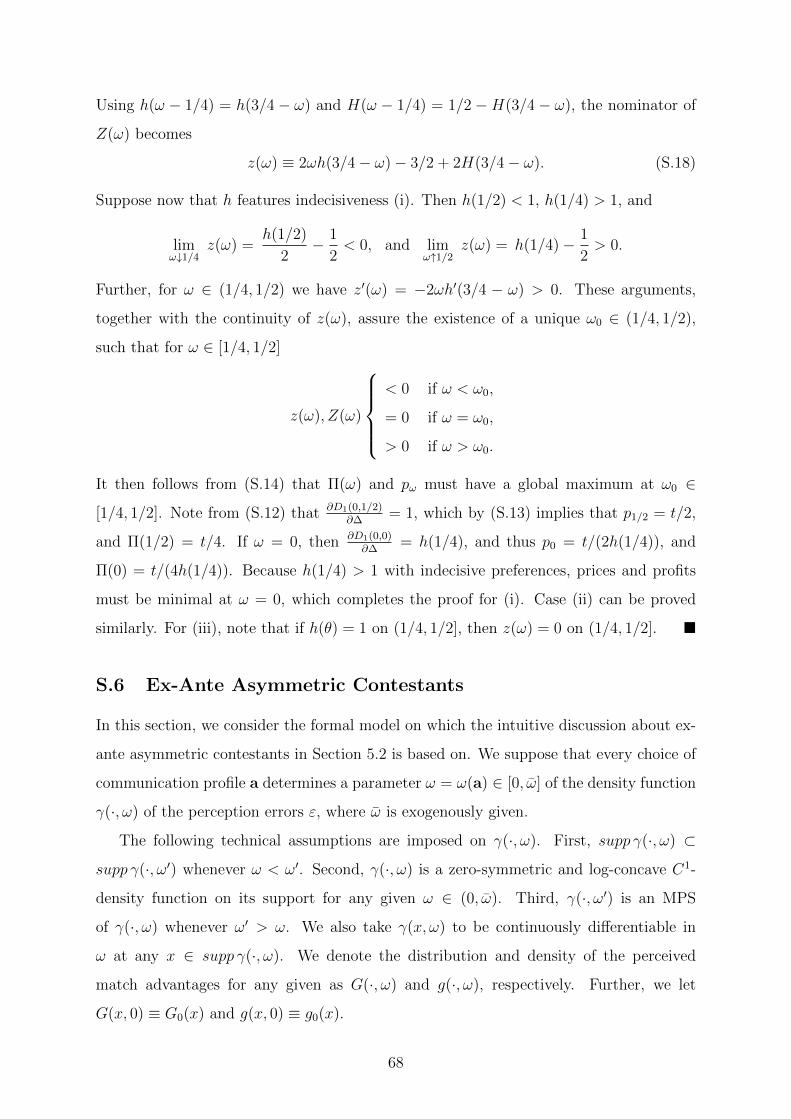
Using h(ω − 1/4) = h(3/4 − ω) and H(ω − 1/4) = 1/2 −H(3/4 − ω), the nominator of

Z(ω) becomes

z(ω) ≡ 2ωh(3/4− ω)− 3/2 + 2H(3/4− ω). (S.18)

Suppose now that h features indecisiveness (i). Then h(1/2) < 1, h(1/4) > 1, and

limω↓1/4

z(ω) =h(1/2)

2− 1

2< 0, and lim

ω↑1/2z(ω) = h(1/4)− 1

2> 0.

Further, for ω ∈ (1/4, 1/2) we have z′(ω) = −2ωh′(3/4 − ω) > 0. These arguments,

together with the continuity of z(ω), assure the existence of a unique ω0 ∈ (1/4, 1/2),

such that for ω ∈ [1/4, 1/2]

z(ω), Z(ω)

< 0 if ω < ω0,

= 0 if ω = ω0,

> 0 if ω > ω0.

It then follows from (S.14) that Π(ω) and pω must have a global maximum at ω0 ∈

[1/4, 1/2]. Note from (S.12) that ∂D1(0,1/2)∂∆

= 1, which by (S.13) implies that p1/2 = t/2,

and Π(1/2) = t/4. If ω = 0, then ∂D1(0,0)∂∆

= h(1/4), and thus p0 = t/(2h(1/4)), and

Π(0) = t/(4h(1/4)). Because h(1/4) > 1 with indecisive preferences, prices and profits

must be minimal at ω = 0, which completes the proof for (i). Case (ii) can be proved

similarly. For (iii), note that if h(θ) = 1 on (1/4, 1/2], then z(ω) = 0 on (1/4, 1/2]. �

S.6 Ex-Ante Asymmetric Contestants

In this section, we consider the formal model on which the intuitive discussion about ex-

ante asymmetric contestants in Section 5.2 is based on. We suppose that every choice of

communication profile a determines a parameter ω = ω(a) ∈ [0, ω] of the density function

γ(·, ω) of the perception errors ε, where ω is exogenously given.

The following technical assumptions are imposed on γ(·, ω). First, supp γ(·, ω) ⊂

supp γ(·, ω′) whenever ω < ω′. Second, γ(·, ω) is a zero-symmetric and log-concave C1-

density function on its support for any given ω ∈ (0, ω). Third, γ(·, ω′) is an MPS

of γ(·, ω) whenever ω′ > ω. We also take γ(x, ω) to be continuously differentiable in

ω at any x ∈ supp γ(·, ω). We denote the distribution and density of the perceived

match advantages for any given as G(·, ω) and g(·, ω), respectively. Further, we let

G(x, 0) ≡ G0(x) and g(x, 0) ≡ g0(x).

68

The payoff functions are given by (2) with R(s1, s2) = 1, where we replace Ga(s1−s2)

by G(s1 − s2, ω) given our notational convention, where G(s1 − s2, ω) =∫ s1−s2−∞ g(s, ω)ds

is the market share of contestant 1 for effort profile (s1, s2). Further, we assume that

C1, C2 are C2-functions with C ′j(s), C′′j (s) > 0 for any s > 0 and Cj(0) = 0, j = 1, 2. We

assume that payoffs are strictly quasi-concave in own strategies for any given ω ∈ [0, ω),

meaning that g′(s1 − s2, ω) − C ′′j (sj) < 0 whenever g(s1 − s2, ω) = C ′j(sj). For a given

ω ∈ [0, ω), an interior effort equilibrium s1(ω), s2(ω) is then determined by the first-order

system

g(s1 − s2, ω) = C1′(s1), g(s1 − s2, ω) = C2

′(s2). (S.19)

In the following we consider ex-ante asymmetry of the contestants in terms of ranked

cost functions, where C ′1(s) < C ′2(s) for any s > 0. We refer to j = 1 as the strong, and

to j = 2 as the weak contestant, respectively. Our main result in this section shows that

the incentive to obfuscate or educate is quite unambiguous for the weak contestant.

Proposition S6 If, for some sufficiently large δ > 0, g0 is strongly indecisive on [−δ, δ],

the weak contestant unambiguously desires maximal agent confusion (ω = ω). If g0 is

strongly polarized on [−δ, δ], the weak contestant unambiguously desires minimal agent

education (ω = 0).

Proof of Proposition S6 We prove the proposition in a serious of lemmas. Note that

in for follow, we take for granted the existence of a unique effort equilibrium s1(ω), s2(ω) >

0 for any given ω ∈ [0, ω).65

Lemma S1 For any given ω ∈ [0, ω], s1(ω) > s2(ω) and Π1(ω) > Π2(ω).

Proof: By (S.19), C ′1(s1) = C ′2(s2) in equilibrium, from which s1 > s2 follows. Equilib-

rium payoffs are Π1(ω) = G(s1− s2, ω)−C1(s1) and Π2(ω) = 1−G(s1− s2, ω)−C2(s2).

The fact that s1 > s2 implies G(s1 − s2, ω) > 1/2. Then

Π1(ω) ≥ 1

2− C1(s2) ≥ 1

2− C2(s2) > Π2(ω),

where the second inequality follows that C1(0) = C2(0) and C ′1(s) < C ′2(s) for all s > 0. �

65Our formal analysis below can be extended to show that, actually, the strong quasi-concavity as-

sumption already assures that at most one equilibrium can exist in the effort game.

69

Define s∆(ω) ≡ s1(ω) − s2(ω). Note that for sufficiently large δ > 0 (which we

assumed), s∆(ω) ∈ [0, δ − ω) ∀ω ∈ [0, ω].

Lemma S2 Suppose that g0 is strongly indecisive (polarized) on supp g0. For any given

x ∈ [0, δ − ω), g(x, ω) is strictly decreasing (increasing) in ω.

Proof: The requirement x ∈ [0, δ − ω) assures that supp gω(x) ⊂ (−δ, δ) for any

ω ∈ (0, ω]. The claims follow from the proof of Theorem 2 by replacing ga′(0) with

g(x, ω′) and ga(0) with g(x, ω) in (A.3). �

Lemma S3 Suppose that g0 is strongly indecisive (polarized) on supp g0. For any given

x ∈ (0, δ − ω), ω, ω′ ∈ [0, ω] with ω < ω′, G(x, ω′) < (>)G(x, ω).

Proof: The claim follows from Lemma S2 because

G(x, ω) =1

2+

∫ x

0

g(s, ω)ds >1

2+

∫ sx

0

g(s, ω′)ds = G(x, ω′). �

Lemma S4 If g0 is strongly indecisive on supp g0, then s′1(ω), s′2(ω) < 0. If g0 is strongly

polarized on supp g0, then s′1(ω), s′2(ω) > 0

Proof: The assumptions imposed in the current model assure that (S.19) is a system of

C1 functions, so by the Implicit Function Theorem, we have for each j = 1, 2,

sj′(ω) =

C−j′′

A

∂g(s∆, ω)

∂ω, A ≡ C1

′′C2′′ + (C1

′′ − C2′′)∂g(s∆, ω)

∂s∆

,

where A > 0 is implied by strong quasi-concavity. Hence sign s′j(ω) = sign(∂g(s∆,ω)

∂ω

),

and the claim for the indecisive case follows because g(s∆, ω) is strictly decreasing in ω

by Lemma S2.66 The claim for the polarized case holds because then g(s∆, ω) is strictly

increasing in ω. �

66Strictly spoken, the strict monotonicity in Lemma S2 allows us only to conclude that ∂g(s∆,ω)∂ω ≤ 0.

As ∂g(s∆,ω)∂ω = 0 can never occur on any arbitrary small interval around ω, we ignore the knife-edge case

where ∂g(s∆,ω0)∂ω0

= 0 for some ω0.

70

Finally, we apply the Envelope Theorem to see how equilibrium payoffs respond to

marginal changes of ω:

Π1′(ω) = −g(s1 − s2, ω)s1

′(ω) +∂G(s1 − s2, ω)

∂ω,

Π2′(ω) = −g(s1 − s2, ω)s2

′(ω)− ∂G(s1 − s2, ω)

∂ω. (S.20)

Because g(·) > 0, Lemmas S3 and S4 imply that Π2(ω) is strictly increasing (decreasing)

on [0, ω] if g0 is strongly indecisive (strongly polarized). �

The comparative statics (S.20) shows that agent confusion increases equilibrium pay-

offs by a competition-softening effect. In the symmetric model, where s1 = s2 and,

accordingly, G(s1 − s2, ω) = 1/2, this is the only force, explaining why both firms un-

ambiguously benefit from agent confusion. By contrast, the market share effect always

works in opposite directions for the two contestants whenever G(s1 − s2, ω) ∈ (1/2, 1),

showing a potential conflict of interest in the contestants’ desire for confusion or educa-

tion. Nevertheless, it turns out that the sensitivity and market share effects always work

in the same direction for the weak, and always in opposite directions for the strong con-

testant. In particular, the weak (strong) contestant always gains (loses) market share if ω

increases in case of indecisive preferences, and vice-versa in case of polarized preferences.

S.7 Ex-Interim Asymmetry

In this section, we consider a simple extension allowing for the possibility that biased

perception errors εa, leading to ex-interim asymmetries of the contestants, may result

as a consequence of the chosen communication strategies. Suppose that A = {0, 1}, so

that A consists of four ordered pairs, associated with four random variables εa, each with

supp (ga) ⊂ supp (g0). Then, aj = 0 means that j communicates in a neutral way, while

aj = 1 means that j’s communication is obfuscating with the possible effect of biasing

perception towards the firm. We assume that ε0,0 = O, ε1,1 6= O is zero-symmetric, and

ε1,0 = −ε0,1. The symmetry of ε1,1 captures that a communication profile where both

contestants seek to bias valuations in their favor (e.g. both exaggerate the valuations of

their offers) results in unbiased agent confusion.67

67For example, ε1,1 always is zero-symmetric if ε1,1 = ε2 − ε1 and ε1, ε2 are iid. In particular, let

εa ≡ ε2a2− ε1

a1, where ε1

a1, ε2a2

are independent. Set εj0 = O, and let ε21 be uniform on [0, ω], and ε1

1 be

71

Contestant 2

𝑎𝑎 = 0 𝑎𝑎 = 1

Contestant 1𝑎𝑎 = 0 Π00 , Π00 Π01 , Π10𝑎𝑎 = 1 Π10 , Π01 Π11 , Π11

Figure S.4: Equilibrium payoffs in effort stage game

Suppose that for any such given εa the effort subgame following εa has a unique effort

equilibrium, with corresponding equilibrium payoffs indicated by Πa, as depicted in the

game matrix of Figure S.4.

In any SPE, the choice of communication profile must induce a Nash equilibrium in

that game. If ε1,0 = ε0,1 is zero-symmetric and ε1,0 6= O, this is just a special case of our

main model and, by Theorem 1, preferences alone are decisive for the type of SPE that

results. It is easily observed that the same equilibrium pattern holds if the bias induced

by aj = 1 is “weak” in the sense that ε1,0 remains close to zero-symmetrically distributed.

Then, the unilateral advantage of a biased communication profile is dominated by the

perception noise it induces. As long as Π00 < (>)Π10 continues to hold, education can

never be (always is) an SPE in case of indecisive (polarized) preferences.

If perception errors are strongly biased in favor of j = 1 if a = (1, 0) is chosen (and

j = 2 is equally favored for a′ = (0, 1)), it becomes conceivable that Π10 > Π00 >

Π01. This reflects a redistribution of the perceived match advantages in favor of j = 1.

Consider first the case of indecisive preferences. Because a potential bias in favor of the

competitor can be annihilated by choosing a = 1, and pure perception noise is beneficial

with indecisive preferences, it follows that Π11 > Π01. Thus, the only equilibrium involves

mutual obfuscation (a1 = a2 = 1), similar to the case with unbiased perception errors.

Now consider the case of polarized preferences, meaning that Π00 > Π11. The type

of SPE now depends crucially on the obfuscation technology. In particular, full agent

education remains the unique equilibrium prediction if consumer education can be uni-

laterally enforced. Then, εa = O whenever a 6= (1, 1), meaning that both contestants

earn Π00, whenever at least one contestant chooses a = 0. Then, any a 6= (1, 1) consti-

tutes a Nash equilibrium in the first stage, and agents are fully educated. If however,

uniform on [−ω, 0], ω > 0. Note that then ε1,1 has a zero-symmetric density (a “tent” distribution) on

[−ω, ω].

72

education cannot be unilaterally enforced, Π10 > Π00 implies that agent education can-

not be sustained as an SPE outcome. The type of equilibrium then depends on whether

Π01 > Π11 or Π01 < Π11. If Π01 < Π11, correcting the bias is more valuable than the loss in

payoffs incurred from mutual obfuscation due to polarized tastes. Then, the contestants

are trapped in a Prisoner’s Dilemma, with mutual obfuscation as the sole equilibrium

outcome, which is both inefficient and harmful for the contestants. If instead Π01 > Π11,

then the contestants end up in a Coordination game with two (pure-strategy) equilibria,

where one contestant earns the rents from a biased communication profile. In sum, agent

preferences play a decisive role for the equilibrium outcome also with potentially biased

communication strategies. In particular, neither a Prisoner’s Dilemma nor a Coordination

game can arise with indecisive tastes.

73