Preference diversity orderings

Un ive rs i t y o f He ide lbe rg

Discussion Paper Series No. 610

Department of Economics

Preference diversity orderings

Alexander Karpov

March 2016

1

Preference diversity orderings

Alexander Karpov1

National Research University Higher School of Economics

E-mail: [email protected]

Postal address: National Research University Higher School of Economics, Department of Economics,

Myasnitskaya str. 20, 101000 Moscow, Russia

Heidelberg University

E-mail: [email protected]

Postal address: Heidelberg University, Department of Economics, Bergheimer Str. 58, 69115 Heidelberg,

Germany

tel.: +49 6221 54-2944

Fax: +49 6221 54-2997

This paper surveys approaches to preference diversity measurement. Applying preference diversity

axiomatics, a generalization of the Alcalde-Unzu and Vorsatz (2016) criterion, is developed. It is shown

that all previously used indices violate this criterion. Two new indices (geometric mean based and leximax-

based) are developed that satisfy a new criterion. Leximax-based orders act as a polarization index and are

compared with Can et al.’s (2015) polarization index. The paper concludes by formulating a new open

question: the preference profile reconstruction conjecture.

JEL Classification: D70.

Keywords: polarization, cohesiveness, ANEC, Leximax, Borda, reconstruction conjecture.

1 The author would like to thank Dmitri Piontkovski for valuable comments and Yuliya Veselova for presented sets of ANECs. The work was partially financed by the International Laboratory of Decision Choice and Analysis (DeCAn Lab) within the Program for Fundamental Research of the National Research University Higher School of Economics.

2

1. Introduction

The diversity of preferences in a group is an aggregative concept representing the lack of

coincidence among individual preferences, level of disagreement, polarization, difficulty of

reaching an agreement, and so on. In some social choice studies (Alcalde-Unzu and Vorsatz 2013,

2016), the term group cohesiveness is used for the opposite situation, i.e., low preference diversity.

This term is borrowed from social psychology, where it describes a broader concept comprising

dynamic, emotional and other aspects (Carron, Brawley 2000; Cota et al. 1995). The term diversity

is borrowed from studies by Hashemi, Endriss (2014), and Gehrlein et al. (2013). In social choice

theory, we consider the terms diversity and cohesiveness as purely opposite concepts without

nuance. In the opinion of the author, diversity is a more neutral term that does not create needless

associations. For brevity, we use term ‘preference diversity’ rather than ‘preference profile

diversity.’

The degree of diversity of preferences in a group is a key parameter in social choice and

matching theories. In social choice models, diverse preferences represent a high degree of conflict

in a group. In general, a low diversity of preferences simplifies many voting problems, reduces the

frequency of Condorcet’s paradox, and prevents successful manipulation. Similarity among

preferences induces higher competition in two-sided matching and house allocation problems. The

degree of similarity of preferences also influences the stability and efficiency of matching

mechanisms.

The importance of preference diversity was discovered in different models. Lepelley and

Valognes (2003) found a positive relationship between strategic manipulation and diversity of

preferences using a homogeneity parameter in the Pólya–Eggenberger model. Studying elections

with three alternatives, Gehrlein et al. (2013) found that increasing the number of possible

preference ranking types increases the probability of strategic manipulation. Gehrlein and Lepelley

(2011, 2015) surveyed the relationship between diversity of preferences and the frequency of

Condorcet’s and other paradoxes. Hałaburda (2010) showed that in two-sided matching market,

unravelling (contracting long before relevant information is available) is more likely to occur when

participants have a higher degree of similar preferences. Boudreau and Knoblauch (2013) studied

the connection between preference diversity and the price of stability in two-sided matching

problems. Manea (2009) found that there is a relationship between the probability that the random

serial dictatorship mechanism is ordinally efficient and the degree of similarity of preferences.

In economic theory, the diversity measurement problem is mainly associated with

biodiversity measurement and other related problems (see survey Nehring, Puppe 2009). This

framework applies a multi-attribute approach, uses only binary dissimilarity information, and

requires an “acyclic” structure of attributes (Nehring, Puppe 2002). The preference diversity

measurement problem has other characteristics and requires its own framework. Despite the

importance of preference diversity measurement, it is novel area of research and still there is no

consensus in such studies.

Our study focuses on ordinal measures of preference diversity. Preference diversity indices

only represent the corresponding ordering of preference profiles. Preference profiles with different

numbers of alternatives or agents are incompatible. There are several axiomatic justifications for

certain preference diversity measures (Alcalde-Unzu and Vorsatz 2013, 2016; Can, Ozken and

3

Strocken 2015). All of these studies start from properties of preference diversity indices, but not

from the properties of preference diversity orderings. The only information they utilize comes

from a weighted tournament matrix. In this paper, we show that such a matrix is not enough for a

well-discernible preference diversity index.

Alcalde-Unzu and Vorsatz’s (2016) paper was motivated by the 3 agents, 3 alternatives

conundrum. They showed that there is no distance-based preference diversity index with an

arithmetic mean aggregator that can represent the correct diversity order on a pair of intuitively

ordered preference profiles. We reinforce this conundrum, investigating a weak order of all 3

agents, 3 alternatives preference profiles, which we call the basic 3 × 3 order. We develop

axiomatics from Hashemi and Endriss’s (2014) survey, adding new axioms and justifying the basic

3 × 3 order by the set of axioms. The ability to represent this order is an aggregated condition for

preference diversity indices. We show that all previously proposed indices fail to represent this

order.

This study does not seek to find a unique preference diversity index that satisfies certain

properties. Different indices are needed for different research goals, but some weak criteria should

be satisfied for all diversity indices and the basic 3 × 3 order becomes this criterion.

We solve the 3 agents, 3 alternatives conundrum by proposing two new preference diversity

orders. One of them is a distance-based preference diversity index with a geometric mean

aggregator, and the second is based on the leximax comparison. The geometric mean-based index

is an alternative to Alcalde-Unzu and Vorsatz’s (2013, 2016) indices and is able to represent the

basic 3 × 3 order. The family of leximax-based indices (and corresponding orders) do not belong

to any class from Hashemi and Endriss’s (2014) survey. These indices are alternatives to Can et

al.’s (2015) polarization index because the maximally polarized preference profiles have the

highest diversity with respect to leximax-based orders. Seeking to increase discernibility power

(the number of anonymous and neutral classes of preference profiles that are not equivalent

according to the index), we introduce iterative reinforcements of leximax orders. Potentially, there

is an index from this family that uniquely characterizes each ANEC of the preference profiles.

Preference profile reconstruction conjecture, which is discussed in the conclusion, uniquely

defines preference profiles from the collection of preference deleted preference profiles. The proof

of this conjecture is an important step in development of strongly discernible order using the

leximax family. This conjecture links this study with graph theory, where the graph reconstruction

conjecture remains one of the classical unsolved problems. In addition to the preference profile

reconstruction conjecture, the domain reconstruction conjecture is discussed.

The remainder of the paper is organized as follows. Section 2 describes preference diversity

axioms and analyzes the 3 agents, 3 alternatives case. Section 3 presents different preference

diversity measures. Section 4 develops leximax preference diversity orderings. Section 5

concludes and describes reconstruction conjectures.

2. Framework

Let a finite set � = {1, … ,�}, � ≥ 2 be the set of alternatives and a finite set � =

{1,… , �}, � ≥ 2 be the set of agents (voters). Each agent � ∈ � has a strict preference �� over �

(linear order). Let ℒ(�) be the set of all possible linear orders over �. An n-tuple of preference

4

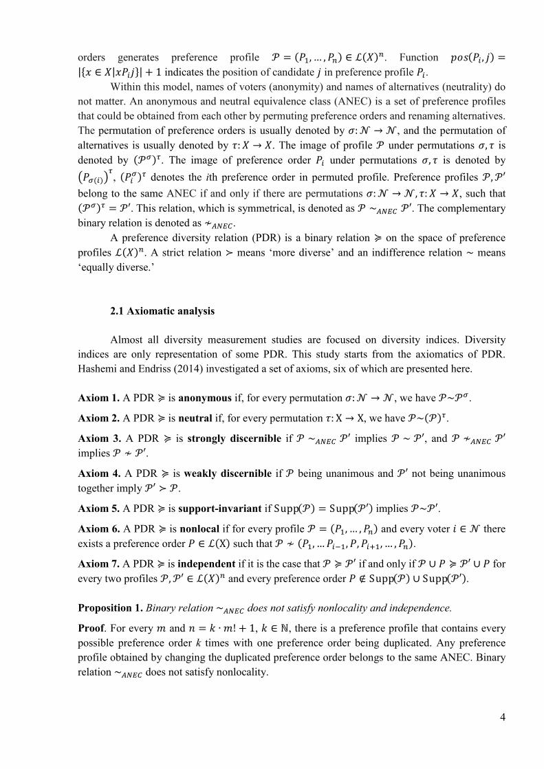
orders generates preference profile � = (��,… , ��) ∈ ℒ(�)�. Function ��(��, �) =

|{� ∈ �|��}|+ 1 indicates the position of candidate � in preference profile ��.

Within this model, names of voters (anonymity) and names of alternatives (neutrality) do

not matter. An anonymous and neutral equivalence class (ANEC) is a set of preference profiles

that could be obtained from each other by permuting preference orders and renaming alternatives.

The permutation of preference orders is usually denoted by �:� → �, and the permutation of

alternatives is usually denoted by �:� → �. The image of profile � under permutations �, � is

denoted by (��)�. The image of preference order �� under permutations �, � is denoted by

��(�)��, (��

�)� denotes the ith preference order in permuted profile. Preference profiles �,�′

belong to the same ANEC if and only if there are permutations �:� → �, �:� → �, such that

(��)� = �′. This relation, which is symmetrical, is denoted as � ∼�� ′. The complementary

binary relation is denoted as ≁��.

A preference diversity relation (PDR) is a binary relation ≽ on the space of preference

profiles ℒ(�)�. A strict relation ≻ means ‘more diverse’ and an indifference relation ∼ means

‘equally diverse.’

2.1 Axiomatic analysis

Almost all diversity measurement studies are focused on diversity indices. Diversity

indices are only representation of some PDR. This study starts from the axiomatics of PDR.

Hashemi and Endriss (2014) investigated a set of axioms, six of which are presented here.

Axiom 1. A PDR ≽ is anonymous if, for every permutation �:� → �, we have �~�� .

Axiom 2. A PDR ≽ is neutral if, for every permutation �:X → X, we have �~(�)�.

Axiom 3. A PDR ≽ is strongly discernible if � ∼�� ′ implies � ∼ �′, and � ≁�� ′

implies � ≁ �′.

Axiom 4. A PDR ≽ is weakly discernible if � being unanimous and �′ not being unanimous

together imply �′≻ �.

Axiom 5. A PDR ≽ is support-invariant if Supp(�) = Supp(�′) implies �~�′.

Axiom 6. A PDR ≽ is nonlocal if for every profile � = (��,… , ��) and every voter � ∈ � there

exists a preference order � ∈ ℒ(X) such that � ≁ (��,…��, �, ��, … , ��).

Axiom 7. A PDR ≽ is independent if it is the case that � ≽ �′ if and only if � ∪ � ≽ �′∪ � for

every two profiles �,�′∈ ℒ(�)� and every preference order � ∉ Supp(�) ∪ Supp(�′).

Proposition 1. Binary relation ∼�� does not satisfy nonlocality and independence.

Proof. For every � and � = � ∙�!+ 1, � ∈ ℕ , there is a preference profile that contains every

possible preference order k times with one preference order being duplicated. Any preference

profile obtained by changing the duplicated preference order belongs to the same ANEC. Binary

relation ∼�� does not satisfy nonlocality.

5

Let � be a preference order with ��…��. Let τ= ��

��…��

��

�� be the

permutation of alternatives. For any � ≥ 5, there is (�, (�)�) ∼�� ((�)�, ((�)�)�), but

(�, (�)�, (((�)�)�)�) ≁�� ((�)�, ((�)�)�, (((�)�)�)�). Binary relation ∼�� does not satisfy

independence.■

Because binary relation ∼�� does not satisfy nonlocality and independence, any

anonymous and neutral PDR does not satisfy nonlocality and independence.

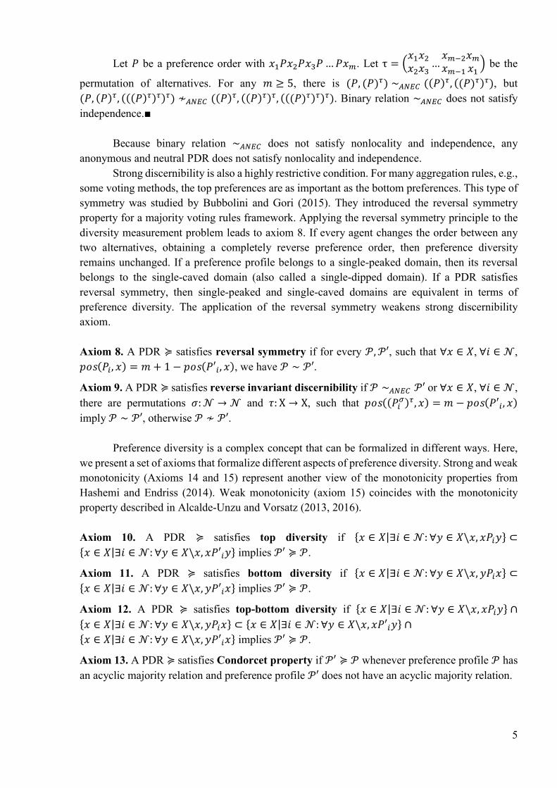
Strong discernibility is also a highly restrictive condition. For many aggregation rules, e.g.,

some voting methods, the top preferences are as important as the bottom preferences. This type of

symmetry was studied by Bubbolini and Gori (2015). They introduced the reversal symmetry

property for a majority voting rules framework. Applying the reversal symmetry principle to the

diversity measurement problem leads to axiom 8. If every agent changes the order between any

two alternatives, obtaining a completely reverse preference order, then preference diversity

remains unchanged. If a preference profile belongs to a single-peaked domain, then its reversal

belongs to the single-caved domain (also called a single-dipped domain). If a PDR satisfies

reversal symmetry, then single-peaked and single-caved domains are equivalent in terms of

preference diversity. The application of the reversal symmetry weakens strong discernibility

axiom.

Axiom 8. A PDR ≽ satisfies reversal symmetry if for every �,�′, such that ∀� ∈ �, ∀� ∈ �,

��(��, �) = � + 1 − ��(�′�, �), we have � ∼ �′.

Axiom 9. A PDR ≽ satisfies reverse invariant discernibility if � ∼�� ′ or ∀� ∈ �, ∀� ∈ �,

there are permutations �:� → � and �:X → X, such that ��((��)�, �) = � − ��(�′�, �)

imply � ∼ �′, otherwise � ≁ �′.

Preference diversity is a complex concept that can be formalized in different ways. Here,

we present a set of axioms that formalize different aspects of preference diversity. Strong and weak

monotonicity (Axioms 14 and 15) represent another view of the monotonicity properties from

Hashemi and Endriss (2014). Weak monotonicity (axiom 15) coincides with the monotonicity

property described in Alcalde-Unzu and Vorsatz (2013, 2016).

Axiom 10. A PDR ≽ satisfies top diversity if {� ∈ �|∃� ∈ �:∀� ∈ �\�, ��} ⊂

{� ∈ �|∃� ∈ �:∀� ∈ �\�, ��′��} implies �′≽ �.

Axiom 11. A PDR ≽ satisfies bottom diversity if {� ∈ �|∃� ∈ �:∀� ∈ �\�, ��} ⊂

{� ∈ �|∃� ∈ �:∀� ∈ �\�, ��′��} implies �′≽ �.

Axiom 12. A PDR ≽ satisfies top-bottom diversity if {� ∈ �|∃� ∈ �:∀� ∈ �\�, ��} ∩

{� ∈ �|∃� ∈ �:∀� ∈ �\�, ��} ⊂ {� ∈ �|∃� ∈ �:∀� ∈ �\�, ��′��} ∩

{� ∈ �|∃� ∈ �:∀� ∈ �\�, ��′��} implies �′≽ �.

Axiom 13. A PDR ≽ satisfies Condorcet property if �′≽ � whenever preference profile � has

an acyclic majority relation and preference profile �′ does not have an acyclic majority relation.

6

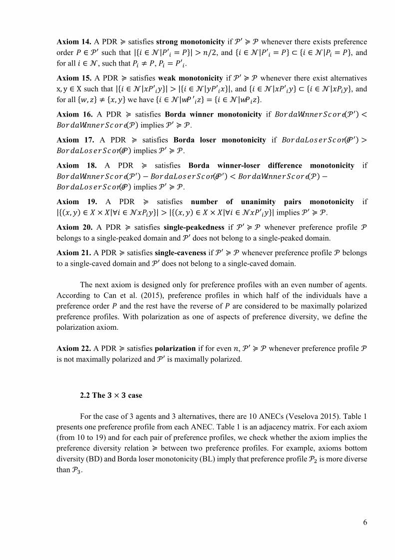
Axiom 14. A PDR ≽ satisfies strong monotonicity if �′≽ � whenever there exists preference

order � ∈ �′ such that |{� ∈ �|�′� = �}|> �/2, and {� ∈ �|�′� = �} ⊂ {� ∈ �|�� = �}, and

for all � ∈ �, such that �� ≠ �, �� = �′�.

Axiom 15. A PDR ≽ satisfies weak monotonicity if �′≽ � whenever there exist alternatives

x, y ∈ X such that |{� ∈ �|��′��}|> |{� ∈ �|��′��}|, and {� ∈ �|��′��} ⊂ {� ∈ �|��}, and

for all {� , �} ≠ {�, �} we have {� ∈ �|��′��} = {� ∈ �|��}.

Axiom 16. A PDR ≽ satisfies Borda winner monotonicity if ��(��) <

��(�) implies �′≽ �.

Axiom 17. A PDR ≽ satisfies Borda loser monotonicity if ��(��) >

��(�) implies �′≽ �.

Axiom 18. A PDR ≽ satisfies Borda winner-loser difference monotonicity if

��(��) − ��(��) < ��(�) −

��(�) implies �′≽ �.

Axiom 19. A PDR ≽ satisfies number of unanimity pairs monotonicity if

|{(�, �) ∈ � × �|∀� ∈ ��}|> |{(�, �) ∈ � × �|∀� ∈ ��′��}| implies �′≽ �.

Axiom 20. A PDR ≽ satisfies single-peakedness if �′≽ � whenever preference profile �

belongs to a single-peaked domain and �′ does not belong to a single-peaked domain.

Axiom 21. A PDR ≽ satisfies single-caveness if �′≽ � whenever preference profile � belongs

to a single-caved domain and �′ does not belong to a single-caved domain.

The next axiom is designed only for preference profiles with an even number of agents.

According to Can et al. (2015), preference profiles in which half of the individuals have a

preference order � and the rest have the reverse of � are considered to be maximally polarized

preference profiles. With polarization as one of aspects of preference diversity, we define the

polarization axiom.

Axiom 22. A PDR ≽ satisfies polarization if for even �, �′≽ � whenever preference profile �

is not maximally polarized and �′ is maximally polarized.

2.2 The � × � case

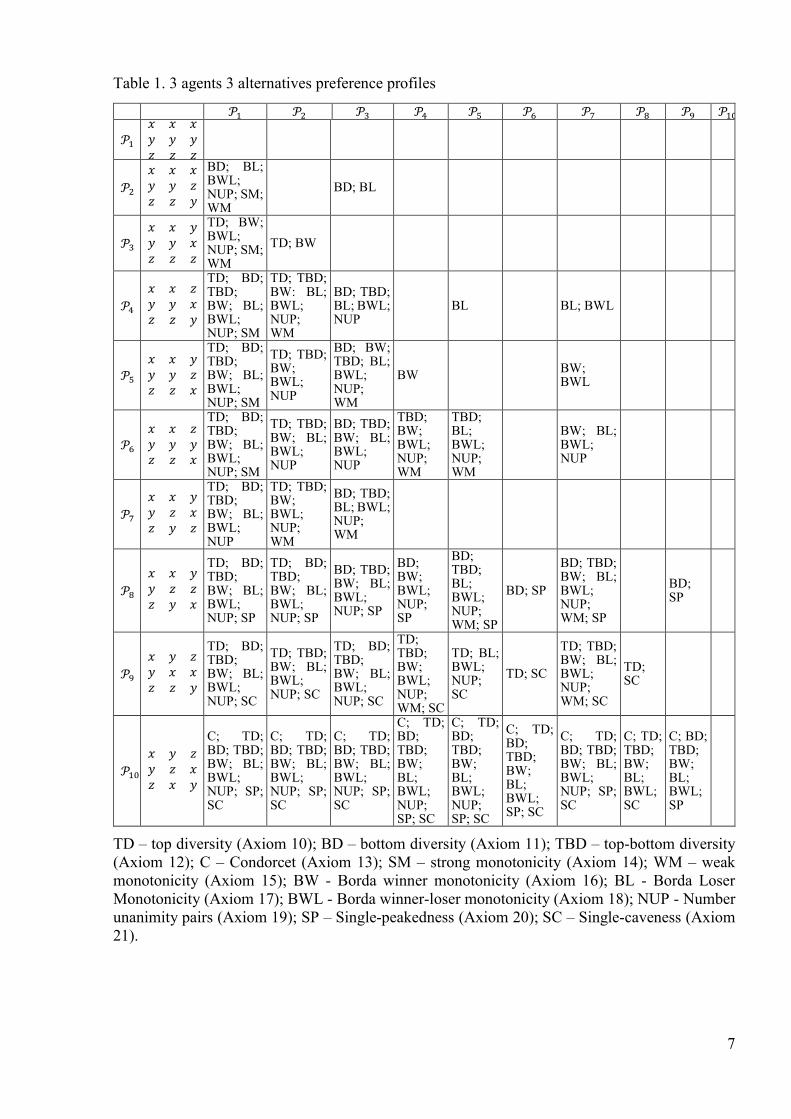
For the case of 3 agents and 3 alternatives, there are 10 ANECs (Veselova 2015). Table 1

presents one preference profile from each ANEC. Table 1 is an adjacency matrix. For each axiom

(from 10 to 19) and for each pair of preference profiles, we check whether the axiom implies the

preference diversity relation ≽ between two preference profiles. For example, axioms bottom

diversity (BD) and Borda loser monotonicity (BL) imply that preference profile �� is more diverse

than ��.

7

Table 1. 3 agents 3 alternatives preference profiles

��

��

��

� � ��

BD; BL; BWL; NUP; SM; WM

BD; BL

��

TD; BW; BWL; NUP; SM; WM

TD; BW

��

� � ��

TD; BD; TBD; BW; BL; BWL; NUP; SM

TD; TBD; BW: BL; BWL; NUP; WM

BD; TBD; BL; BWL; NUP

BL BL; BWL

��

� � ��


TD; TBD; BW; BWL; NUP

BD; BW; TBD; BL; BWL; NUP; WM

BW BW; BWL

��


TD; TBD; BW; BL; BWL; NUP

BD; TBD; BW; BL; BWL; NUP

TBD; BW; BWL; NUP; WM

TBD; BL; BWL; NUP; WM

BW; BL; BWL; NUP

��

� � ��

TD; BD; TBD; BW; BL; BWL; NUP

TD; TBD; BW; BWL; NUP; WM

BD; TBD; BL; BWL; NUP; WM

��

� � ��

TD; BD; TBD; BW; BL; BWL; NUP; SP

TD; BD; TBD; BW; BL; BWL; NUP; SP

BD; TBD; BW; BL; BWL; NUP; SP

BD; BW; BWL; NUP; SP

BD; TBD; BL; BWL; NUP; WM; SP

BD; SP

BD; TBD; BW; BL; BWL; NUP; WM; SP

BD; SP

��

� � ��

TD; BD; TBD; BW; BL; BWL; NUP; SC

TD; TBD; BW; BL; BWL; NUP; SC

TD; BD; TBD; BW; BL; BWL; NUP; SC

TD; TBD; BW; BWL; NUP; WM; SC

TD; BL; BWL; NUP; SC

TD; SC

TD; TBD; BW; BL; BWL; NUP; WM; SC

TD; SC

��

� � ��

C; TD; BD; TBD; BW; BL; BWL; NUP; SP; SC





C; TD; BD; TBD; BW; BL; BWL; SP; SC


C; TD; TBD; BW; BL; BWL; SC

C; BD; TBD; BW; BL; BWL; SP

TD – top diversity (Axiom 10); BD – bottom diversity (Axiom 11); TBD – top-bottom diversity (Axiom 12); C – Condorcet (Axiom 13); SM – strong monotonicity (Axiom 14); WM – weak monotonicity (Axiom 15); BW - Borda winner monotonicity (Axiom 16); BL - Borda Loser Monotonicity (Axiom 17); BWL - Borda winner-loser monotonicity (Axiom 18); NUP - Number unanimity pairs (Axiom 19); SP – Single-peakedness (Axiom 20); SC – Single-caveness (Axiom 21).

8

Each axiom represents its own version of the preference diversity concept. Axioms 10-21

induce different binary relations. There are no two equal binary relations. For some pairs of

preference profiles, axioms agree with each other, while others do not. There is no linear order

satisfying all axioms 10-21; it is an impossibility result for strongly discernible aggregation. The

most discernible weak order that satisfies axioms 10-21 is the order with 7 indifference sets:

�� ≻ ��∿�� ≻ �� ≻ ��∿�� ≻ �� ≻ ��∿�� ≻ ��.

Let us call this PDR the basic � × � PDR. This order aggregates all constraints from

axioms 10-21 for the 3 × 3 case. Because there is strong support from several axioms for each

relation in this order, the basic 3 × 3 PDR is robust. Apart from satisfying axioms 10-21, this order

satisfies nonlocality (axiom 6), and reverse invariant discernibility (axiom 9).

In one motivating example, Alcalde-Unzu and Vorsatz (2016) compared preference

profiles �� and ��. They argued that �� ≻ �� and found that all distance based measures with an

arithmetic mean aggregator violate �� ≻ ��. This simple condition helped considerably to reduce

the set of reasonable preference diversity measures. The basic 3×3 PDR is a generalization of

Alcalde-Unzu and Vorsatz’s (2016) motivating example. In the next section, the ability to

represent the basic 3×3 PDR is used as a robust criterion for preference diversity indices. If the

preference diversity index fails to represent this order, then the PDR generated by this index

violates one or more axioms from axioms 10-21. This criterion is weaker than the strong

discernibility axiom, which requires 10 indifference sets for the 3 × 3 case.

Eliminating several axioms, it is possible to design a strongly discernible PDR. In many

social choice and matching problems, top preferences are more important than bottom preferences.

Hence, top diversity and Borda winner monotonicity are more important than bottom diversity and

Borda loser monotonicity. Eliminating bottom diversity, Borda loser monotonicity, and single-

peakness, we obtain:

�� ≻ �� ≻ �� ≻ �� ≻ �� ≻ �� ≻ �� ≻ �� ≻ �� ≻ ��.

This order is not robust. Some relations in this order are supported by only one axiom.

Changing one axiom to another or adding new axioms changes this order. For example, from

single-peakedness we have �� ≽ ��. We do not consider this order as unique and instead desire a

strict order for the 3 × 3 case.

3. Preference diversity indices

The preference diversity index (PDI) is a real valued function Δ:ℒ(�)� → ℝ that respects

Δ(P,… , P) = 0. The preference diversity index represents PDR ≽ if Δ(��) ≥ Δ(��) ⟺ �� ≽

��. We will say that PDI satisfies axiom x if the corresponding PDR satisfies axiom x.

This section follows Hashemi and Endriss’s (2014) survey of PDI types, although it does

not define disjoint classes. Some indices belong to the several classes. Hashemi and Endriss (2014)

argued that non e of the PDIs considered in their paper satisfied strong discernibility. We

generalize this result and focus on reverse invariant discernibility.

9

3.1 Support -based PDI (Hashemi, Endriss, 2014)

For a given � ≤ �, the support-based PDI Δ�� =

|{� ∈ ℒ�(�)|� ⊆ �� ∈ �}|− ��, where ℒ�(�) is the set of k alternatives of linear

orders over X.

Propositions 2 and 3 shows poor discernibility properties of the support-based PDI.

Proposition 2. For � ≥ 4, support-based PDI does not satisfy reverse invariant discernibility.

Proof. Consider two preference profiles �� = ��,… , �� ,�′��

�, �� = ��, … , �� ,��, �′��

�, with

� ≠ ��. These preference profiles do not belong to the same anonymous and neutral equivalence

class, but they have identical support with Δ�� (��) = Δ��

� (��).■

Proposition 3. The basic 3 × 3 PDR cannot be represented by support-based PDI.

Proof. Δ�� generates 3 indifference classes (1, 2, or 3 types of different linear orders). Δ��

�

generates 4 indifference classes (3,4,5,6 types of different linear orders). The basic 3 × 3 PDR

generates 7 indifference classes. Therefore, it cannot be represented by Δ�� , Δ��

� . ■

3.2 Distance based PDI (Hashemi, Endriss, 2014)

For a given distance δ:ℒ(�) × ℒ(�) → ℝ and aggregation operator Φ:ℝ�(��)/� → ℝ, the

distance based PDI Δ��,� maps any given profile � ∈ ℒ(�)� to the following value:

Δ��,� (�) = Φ(�(��, ��)|�, � ∈ �� ℎ � < �).

For every �, ��, �′′∈ ℒ(�) a distance function satisfies the following four conditions:

1) δ(P, P�) ≥ 0 (nonnegativity),

2) δ(P, P�) = 0 if and only if P = P� (identity of indiscernibles),

3) δ(P, P�) = δ(P′, P) (symmetry),

4) δ(P, P�′) ≤ δ(P, P�) + δ(P′, P��) (triangle inequality),

5) for every permutation τ: X → X, we have δ(�, �′) = δ��(�), �(�′)� (neutrality).

Different examples of distances between preference orders are presented in Can (2014),

Elkind et al. (2015), and Mescanen, and Nurmi (2008). Hashemi and Endriss (2014) also proposed

a compromise-based PDI as an aggregation of distances between preference orders and a

compromise order. Any compromise-based PDI can be represented in the form of a distance-based

PDI, redefining the distance measure as:

δ′(P, P�) = 0 if P = P′,

δ′(P, P�) = δ(P, P��) + δ(P��, P�).

Despite having a variety of distances and aggregators, the distance-based PDI does not

satisfy reverse invariant discernibility.

10

Proposition 4. For � ≥ 4, the distance-based PDI does not satisfy reverse invariant

discernibility.

Proof. Let � be a preference order with ��…��. Let us define permutations as:

τ� = ��

��…��

��

��

��

��

�,τ� = ��

��

��…��

��

��

��

��

�.

For � ≥ 4, preference profile �� = (�,… , �, (�)�� ), is not equivalent to �� = (�,… , �, (�)�� )

with respect to anonymity, neutrality and reverse invariance. Because of distance neutrality, we

obtain �(�, (�)��) = �((�)��, ((�)��)��) = �((�)��, P) = �(P, (�)��), hence

Δ��,� (��) = Δ��

�,� (��).■

Alcalde-Unzu and Vorsatz (2016) showed that the distance-based PDI with an arithmetic

mean aggregator cannot represent relation �� ≻ ��. Other aggregators meet the challenge.

Moreover, the basic 3 × 3 PDR can be represented by distance-based PDI, as shown in the next

subsection with the new investigated index.

3.2.1 Geometric mean-based index (GM)

Let us define a slightly modified Kendall rank distance (swap distance):

δ(P, P�) = 0 if P = P′,

δ(P, P�) = |{(�, �) ∈ � × �|��, ��′�}|+ 0.5.

All five conditions for the distance measure are satisfied. For the 3 alternatives case, we have:

� ��,�� = 0, � �

��,

�� = � �

��,�� = 1.5, � �

��,�� = � �

��,

�� = 2.5, � �

��,�� = 3.5.

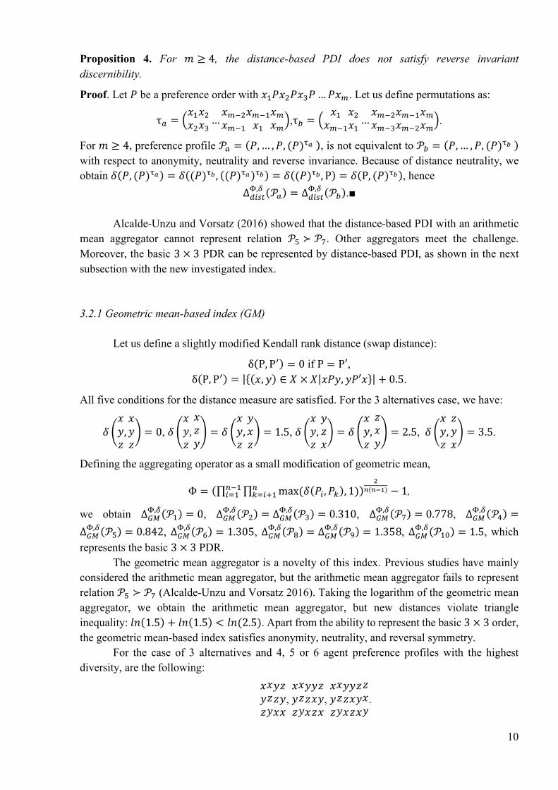
Defining the aggregating operator as a small modification of geometric mean,

Φ = (∏ ∏ max (�(��, ��), 1)��

�� )

�

�(��) − 1,

we obtain Δ��,�(��) = 0, Δ��

�,�(��) = Δ��,�(��) = 0.310, Δ��

�,�(��) = 0.778, Δ��,�(��) =

Δ��,�(��) = 0.842, Δ��

�,�(��) = 1.305, Δ��,�(��) = Δ��

�,�(��) = 1.358, Δ��,�(��) = 1.5, which

represents the basic 3 × 3 PDR.

The geometric mean aggregator is a novelty of this index. Previous studies have mainly

considered the arithmetic mean aggregator, but the arithmetic mean aggregator fails to represent

relation �� ≻ �� (Alcalde-Unzu and Vorsatz 2016). Taking the logarithm of the geometric mean

aggregator, we obtain the arithmetic mean aggregator, but new distances violate triangle

inequality: ��(1.5) + ��(1.5) < �� (2.5). Apart from the ability to represent the basic 3 × 3 order,

the geometric mean-based index satisfies anonymity, neutrality, and reversal symmetry.

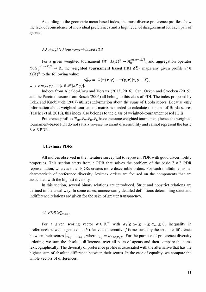
For the case of 3 alternatives and 4, 5 or 6 agent preference profiles with the highest

diversity, are the following:

��

��

��

��

, ��

��

��

��

��

, ��

��

��

��

��

��

.

11

According to the geometric mean-based index, the most diverse preference profiles show

the lack of coincidence of individual preferences and a high level of disagreement for each pair of

agents.

3.3 Weighted tournament-based PDI

For a given weighted tournament �� : ℒ(�)� → ℕ��(��)/�

, and aggregation operator

Φ:ℕ��(��)/�

→ ℝ, the weighted tournament based PDI Δ�� maps any given profile � ∈

ℒ(�)� to the following value:

Δ�� = Φ(�(�, �) − �(�, �)|�, � ∈ �),

where �(�, �) = |{� ∈ �|��}|.

Indices from Alcalde-Unzu and Vorsatz (2013, 2016), Can, Ozken and Strocken (2015),

and the Pareto measure from Bosch (2006) all belong to this class of PDI. The index proposed by

Celik and Knoblauch (2007) utilizes information about the sums of Borda scores. Because only

information about weighted tournament matrix is needed to calculate the sums of Borda scores

(Fischer et al. 2016), this index also belongs to the class of weighted-tournament based PDIs.

Preference profiles ��, ��, ��, �� have the same weighted tournament; hence the weighted

tournament-based PDI do not satisfy reverse invariant discernibility and cannot represent the basic

3 × 3 PDR.

4. Leximax PDRs

All indices observed in the literature survey fail to represent PDR with good discernibility

properties. This section starts from a PDR that solves the problem of the basic 3 × 3 PDR

representation, whereas other PDRs creates more discernible orders. For each multidimensional

characteristic of preference diversity, leximax orders are focused on the components that are

associated with the highest diversity.

In this section, several binary relations are introduced. Strict and nonstrict relations are

defined in the usual way. In some cases, unnecessarily detailed definitions determining strict and

indifference relations are given for the sake of greater transparency.

4.1 PDR ≽ ��_��

For a given scoring vector � ∈ ℝ� with �� ≥ �� ≥ ⋯ ≥ �� ≥ 0, inequality in

preferences between agents � and � relative to alternative � is measured by the absolute difference

between their scores ��,� − ��,��, where ��,� = ��(��,�). For the purpose of preference diversity

ordering, we sum the absolute differences over all pairs of agents and then compare the sums

lexicographically. The diversity of preference profile is associated with the alternative that has the

highest sum of absolute difference between their scores. In the case of equality, we compare the

whole vectors of differences.

12

Let a vector �(�) = ��,� − ��,��,�∈�,��,�∈� be the ��(� − 1)/2-dimensional vector of

absolute differences between individual scores. Vector �(�) is a raw data for diversity

measurement. Let a vector �(�) = �∑ ∑ ��,� − ��,��

��

�∈� be the �-dimensional vector of

the sums of absolute differences between individual scores. Vector �(�) is the vector of diversities

of alternatives’ scores.

The leximax relation ≽ � on ℝ� is defined as follows. For any � = ��, … , ��∈ ℝ�, let

�∗ = ��∗, … , ��

∗�∈ ℝ� be a permutation of the coordinates of vector � in the decreasing

order: ��∗ ≥ ⋯ ≥ ��

∗ . If there is a � ∈ {1, … , �} such that ��∗ > ��

∗, while ��∗ = ��

∗ for all � < �, then

� ≻ � �. If ��∗ = ��

∗ for all � ∈ {1,… , �}, then � ∼� �.

Leximax PDR ≽ ��_�� (� is a given scoring vector) is defined by the following rule, which

includes three conditions:

1. If �(�) ≻ � �(�′), then � ≻��_�� ′;

2. If �(�) ∼� �(�′) and �(�) ≻ � �(�′), then � ≻��_�� ′;

3. If �(�) ∼� �(�′) and �(�) ∼� �(�′), then � ∼��_�� ′.

First, preference profiles are compared using the diversity of an alternative with the most

diverse scores. If the sums of the absolute differences between individual scores are equal for all

alternatives, then preference profiles are compared using the highest absolute differences between

individual scores. Vector �(�) includes aggregated information. Leximax comparison of �(�) is

robust and has clear interpretation. Only in the case of equality should we consider raw data �(�).

Even considering �(�), not all preference profiles would be ordered.

In the 3 × 3 case, PDR ≽ ��_�� with Borda scores coincides with the basic 3 × 3 PDR.

Other scores’ vectors also do not generate any strongly discernible order. Preference profiles

��,�� have permuted vectors �(�), �(�), then �(��) ∼� �(��) and �(��) ∼� �(��).

The following preference profiles are examples of preference profiles with the highest

diversity according to PDR ≽ ��_�� , with Borda scores for different numbers of agents and

alternatives:

��

��

��

��

, ��

��

��

��

��

,

��

��

��

��

��

��

;

��

��

��

,

��

��

��

��

,

��

��

��

��

��

,

��

��

��

��

��

��

.

Proposition 5. PDR ≽ ��_�� with Borda scores satisfies anonymity, neutrality, reversal

symmetry, and polarization.

Proof. Because binary relation ≽ � and all functions defined above are anonymous and neutral,

PDR ≽ ��_�� is anonymous and neutral.

If �′ is the reverse of �, then �(�) ∼� �(�′) and �(�) ∼� �(�′), from which follows

� ∼��_�� ′.

Let � be even. Let �� = |{� ∈ �|��(��, �) = �}| be the number of preference orders,

which have alternative � on position �. Let preference profile � be a preference profile with the

13

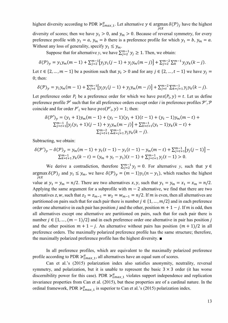
highest diversity according to PDR ≽ ��_�� . Let alternative � ∈ argmax

�∈��(�)� have the highest

diversity of scores; then we have �� > 0, and �� > 0. Because of reversal symmetry, for every

preference profile with �� = �, �� = � there is a preference profile for which �� = �, �� = �.

Without any loss of generality, specify �� ≤ ��.

Suppose that for alternative y, we have ∑ �� ≥ 1. Then, we obtain:

�(�)� = ��(� − 1) + ∑ ��(� − 1) + ��(� − �)�� + ∑ ∑ ��(� − �)��

�� .

Let � ∈ {2,… ,� − 1} be a position such that �� > 0 and for any � ∈ {2, … , � − 1} we have �� =

0; then:

�(�)� = ��(� − 1) + ∑ ��(� − 1) + ��(� − �)�� + ∑ ∑ ��(� − �)��

�� .

Let preference order �� be a preference order for which we have ��(��, �) = �. Let us define

preference profile �′ such that for all preference orders except order i in preference profiles ��,�

coincide and for order �′� we have ��(�′�, �) = 1; then:

�(�′)� = (�� + 1)��(� − 1) + (�� − 1)(�� + 1)(� − 1) + (�� − 1)��(� − �) +

∑ ��(�� + 1)(� − 1) + ��(� − �)�� + ∑ (�� − 1)��(� − �)��

�� +

∑ ∑ ��(� − �)��

�� .

Subtracting, we obtain:

�(��)� − �(�)� = ��(� − 1) + ��(� − 1) − ��(� − 1) − ��(� − �) + ∑ ��(� − 1)�� −

∑ ��(� − �)�� = (�� + �� − ��)(� − 1) + ∑ ��(� − 1)��

�� > 0.

We derive a contradiction, therefore ∑ �� = 0. For alternative y, such that � ∈

argmax�∈�

�(�)� and �� ≤ ��, we have �(�)� = (� − 1)��(� − ��), which reaches the highest

value at �� = �� = �/2. There are two alternatives �, �, such that �� = �� = �� = �� = �/2.

Applying the same argument for a subprofile with � − 2 alternative, we find that there are two

alternatives �, � , such that �� = �� = �� = �� = �/2. If � is even, then all alternatives are

partitioned on pairs such that for each pair there is number � ∈ {1,… ,�/2} and in each preference

order one alternative in each pair has position � and the other, position � + 1 − �. If � is odd, then

all alternatives except one alternative are partitioned on pairs, such that for each pair there is

number � ∈ {1,… , (� − 1)/2} and in each preference order one alternative in pair has position �

and the other position � + 1 − �. An alternative without pairs has position (� + 1)/2 in all

preference orders. The maximally polarized preference profile has the same structure; therefore,

the maximally polarized preference profile has the highest diversity. ■

In all preference profiles, which are equivalent to the maximally polarized preference

profile according to PDR ≽ ��_�� , all alternatives have an equal sum of scores.

Can et al.’s (2015) polarization index also satisfies anonymity, neutrality, reversal

symmetry, and polarization, but it is unable to represent the basic 3 × 3 order (it has worse

discernibility power for this case). PDR ≽ ��_�� violates support independence and replication

invariance properties from Can et al. (2015), but these properties are of a cardinal nature. In the

ordinal framework, PDR ≽ ��_�� is superior to Can et al.’s (2015) polarization index.

14

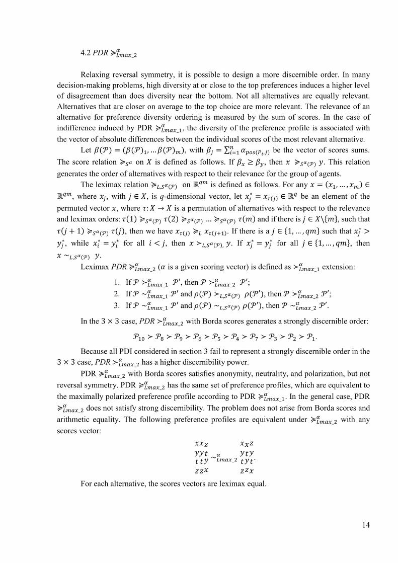
4.2 PDR ≽ ��_��

Relaxing reversal symmetry, it is possible to design a more discernible order. In many

decision-making problems, high diversity at or close to the top preferences induces a higher level

of disagreement than does diversity near the bottom. Not all alternatives are equally relevant.

Alternatives that are closer on average to the top choice are more relevant. The relevance of an

alternative for preference diversity ordering is measured by the sum of scores. In the case of

indifference induced by PDR ≽ ��_�� , the diversity of the preference profile is associated with

the vector of absolute differences between the individual scores of the most relevant alternative.

Let �(�) = (�(�)�, …�(�)�), with �� = ∑ ��(��,�)�� be the vector of scores sums.

The score relation ≽ �� on � is defined as follows. If �� ≥ ��, then � ≽ ��(�) �. This relation

generates the order of alternatives with respect to their relevance for the group of agents.

The leximax relation ≽ �,��(�) on ℝ�� is defined as follows. For any � = (��, … , ��) ∈

ℝ��, where ��, with � ∈ �, is q-dimensional vector, let ��∗ = ��(�) ∈ ℝ� be an element of the

permuted vector �, where �:� → � is a permutation of alternatives with respect to the relevance

and leximax orders: �(1) ≽ ��(�) �(2) ≽ ��(�) … ≽ ��(�) �(�) and if there is � ∈ �\{�}, such that

�(� + 1) ≽ ��(�) �(�), then we have ��(�) ≽ � ��(��). If there is a � ∈ {1,… , ��} such that ��∗ >

��∗, while ��

∗ = ��∗ for all � < �, then � ≻ �,��(�), �. If ��

∗ = ��∗ for all � ∈ {1,… , ��}, then

� ∼�,��(�) �.

Leximax PDR ≽ ��_�� (� is a given scoring vector) is defined as ≻ ��_�

� extension:

1. If � ≻��_�� ′, then � ≻��_�

� �′;

2. If � ∼��_�� ′ and �(�) ≻ �,��(�) �(�′), then � ≻��_�

� �′;

3. If � ∼��_�� ′ and �(�) ∼�,��(�) �(�′), then � ∼��_�

� �′.

In the 3 × 3 case, PDR ≻ ��_�� with Borda scores generates a strongly discernible order:

�� ≻ �� ≻ �� ≻ �� ≻ �� ≻ �� ≻ �� ≻ �� ≻ �� ≻ ��.

Because all PDI considered in section 3 fail to represent a strongly discernible order in the

3 × 3 case, PDR ≻ ��_�� has a higher discernibility power.

PDR ≽ ��_�� with Borda scores satisfies anonymity, neutrality, and polarization, but not

reversal symmetry. PDR ≽ ��_�� has the same set of preference profiles, which are equivalent to

the maximally polarized preference profile according to PDR ≽ ��_�� . In the general case, PDR

≽ ��_�� does not satisfy strong discernibility. The problem does not arise from Borda scores and

arithmetic equality. The following preference profiles are equivalent under ≽ ��_�� with any

scores vector:

��

��

��

∼��_��

��

��

��

.

For each alternative, the scores vectors are leximax equal.

15

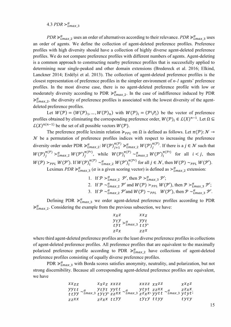
4.3 PDR ≻ ��_��

PDR ≽ ��_�� uses an order of alternatives according to their relevance. PDR ≽ ��_�

� uses

an order of agents. We define the collection of agent-deleted preference profiles. Preference

profiles with high diversity should have a collection of highly diverse agent-deleted preference

profiles. We do not compare preference profiles with different numbers of agents. Agent-deleting

is a common approach to constructing nearby preference profiles that is successfully applied to

determining near single-peaked and other domain extensions (Bredereck et al. 2016; Elkind,

Lanckner 2014; Erdélyi et al. 2013). The collection of agent-deleted preference profiles is the

closest representation of preference profiles in the simpler environment of n-1 agents’ preference

profiles. In the most diverse case, there is no agent-deleted preference profile with low or

moderately diversity according to PDR ≽ ��_�� . In the case of indifference induced by PDR

≽ ��_�� , the diversity of preference profiles is associated with the lowest diversity of the agent-

deleted preference profiles.

Let � (�) = (� (�)�,… , � (�)�) with � (�)� = (�\��) be the vector of preference

profiles obtained by eliminating the corresponding preference order, � (�)� ∈ ℒ(�)��. Let Ω ⊆

ℒ(�)�(��) be the set of all possible vectors � (�).

The preference profile leximin relation ≽�� on Ω is defined as follows. Let �(�):� →

� be a permutation of preference profiles indices with respect to increasing the preference

diversity order under PDR ≽ ��_�� : � (�)��

�(�)≽ ��_�� (�)�

�(�). If there is a � ∈ � such that

� (�)��(�)

≻ ��_�� (�′)�

�(��), while � (�)�

�(�)∼ ��_�� (�′)�

�(��) for all � < �, then

� (�) ≻ �� (�′). If � (�)��(�)

∼ ��_�� (�′)�

�(��) for all � ∈ �, then � (�) ∼�� (�′).

Leximax PDR ≽ ��_�� (� is a given scoring vector) is defined as ≻ ��_�

� extension:

1. If � ≻ ��_�� ′, then � ≻��_�

� �′;

2. If � ∼��_�� ′ and � (�) ≻ �� (�′), then � ≻��_�

� �′;

3. If � ∼��_�� ′and � (�) ∼�� (�′), then � ∼��_�

� �′.

Defining PDR ≽ ��_�� we order agent-deleted preference profiles according to PDR

≽ ��_�� . Considering the example from the previous subsection, we have:

��

��

��

≻ ��_��

��

��

��

,

where third agent-deleted preference profiles are the least diverse preference profiles in collections

of agent-deleted preference profiles. All preference profiles that are equivalent to the maximally

polarized preference profile according to PDR ≽ ��_�� have collections of agent-deleted

preference profiles consisting of equally diverse preference profiles.

PDR ≽ ��_�� with Borda scores satisfies anonymity, neutrality, and polarization, but not

strong discernibility. Because all corresponding agent-deleted preference profiles are equivalent,

we have

��

��

��

��

∼��_��

��

��

��

��

,

��

��

��

��

∼ ��_��

��

��

��

��

,

��

��

��

��

∼��_��

��

��

��

��

;

16

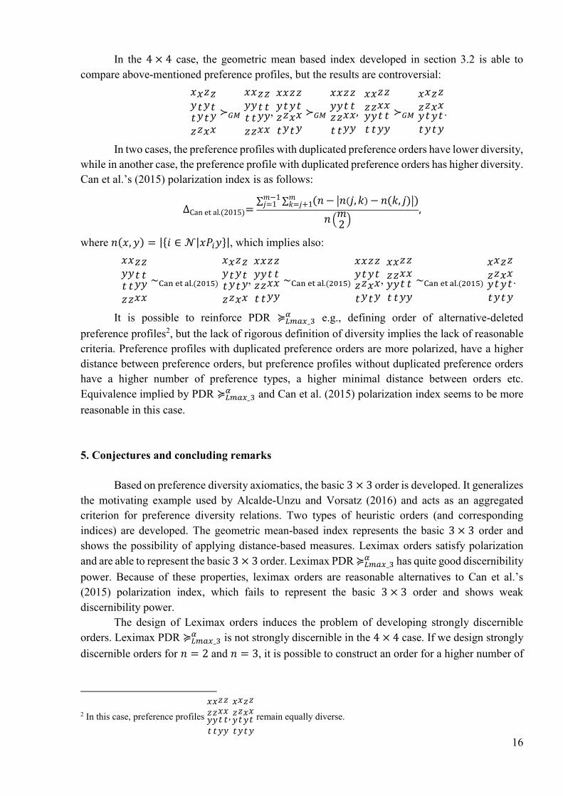
In the 4 × 4 case, the geometric mean based index developed in section 3.2 is able to

compare above-mentioned preference profiles, but the results are controversial:

��

��

��

��

≻��

��

��

��

��

,

��

��

��

��

≻��

��

��

��

��

,

��

��

��

��

≻��

��

��

��

��

.

In two cases, the preference profiles with duplicated preference orders have lower diversity,

while in another case, the preference profile with duplicated preference orders has higher diversity.

Can et al.’s (2015) polarization index is as follows:

∆Can et al.(2015)=∑ ∑ (� − ��(�, �) − �(�, �)��

�=�+ 1�−1�=1 )

��2�,

where �(�, �) = |{� ∈ �|��}|, which implies also:

��

��

��

��

∼�� .(��)

��

��

��

��

,

��

��

��

��

∼�� .(��)

��

��

��

��

,

��

��

��

��

∼�� .(��)

��

��

��

��

.

It is possible to reinforce PDR ≽ ��_�� e.g., defining order of alternative-deleted

preference profiles2, but the lack of rigorous definition of diversity implies the lack of reasonable

criteria. Preference profiles with duplicated preference orders are more polarized, have a higher

distance between preference orders, but preference profiles without duplicated preference orders

have a higher number of preference types, a higher minimal distance between orders etc.

Equivalence implied by PDR ≽ ��_�� and Can et al. (2015) polarization index seems to be more

reasonable in this case.

5. Conjectures and concluding remarks

Based on preference diversity axiomatics, the basic 3 × 3 order is developed. It generalizes

the motivating example used by Alcalde-Unzu and Vorsatz (2016) and acts as an aggregated

criterion for preference diversity relations. Two types of heuristic orders (and corresponding

indices) are developed. The geometric mean-based index represents the basic 3 × 3 order and

shows the possibility of applying distance-based measures. Leximax orders satisfy polarization

and are able to represent the basic 3 × 3 order. Leximax PDR ≽ ��_�� has quite good discernibility

power. Because of these properties, leximax orders are reasonable alternatives to Can et al.’s

(2015) polarization index, which fails to represent the basic 3 × 3 order and shows weak

discernibility power.

The design of Leximax orders induces the problem of developing strongly discernible

orders. Leximax PDR ≽ ��_�� is not strongly discernible in the 4 × 4 case. If we design strongly

discernible orders for � = 2 and � = 3, it is possible to construct an order for a higher number of

2 In this case, preference profiles

��

��

��

��

,

��

��

��

��

remain equally diverse.

17

agents by iterative procedure. If the following conjecture holds, then this order would be strongly

discernible.

Preference profile reconstruction conjecture. For any two preference profiles �,�′∈ ℒ(�)�

with at least four agents, if agent-deleted preference profiles collections are equivalent with

respect to ~��, then �~��′.

Mathematically, this conjecture is closely related to the graph reconstruction conjecture

formulated by P. Kelly and S. Ulam in 1941. There are two main versions of the conjecture: any

two graphs with at least three vertices and the same vertex-deleted subgraph collections are

isomorphic; and any two graphs with at least four edges and the same edge-deleted subgraph

collections are isomorphic. A computer search has verified the reconstruction conjecture for

graphs with nine or fewer vertices (Manvel 2000). The preference profile reconstruction conjecture

can help to develop a strongly discernible index and deepen our knowledge of the structure of

ANECs.

Because in the 3 × 3 case, agent-deleted preference profile collections for ��,�� are

equivalent, the preference profile reconstruction conjecture is false for � = 3. For the cases of 4

agents and 3 alternatives (24 ANECs) and 5 agents and 3 alternatives (42 ANECs), the preference

profile reconstruction conjecture holds.

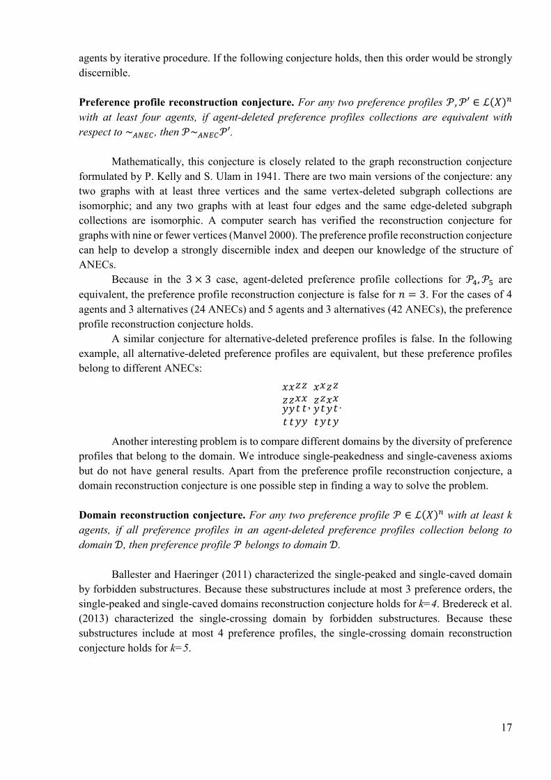
A similar conjecture for alternative-deleted preference profiles is false. In the following

example, all alternative-deleted preference profiles are equivalent, but these preference profiles

belong to different ANECs:

��

��

��

��

,

��

��

��

��

.

Another interesting problem is to compare different domains by the diversity of preference

profiles that belong to the domain. We introduce single-peakedness and single-caveness axioms

but do not have general results. Apart from the preference profile reconstruction conjecture, a

domain reconstruction conjecture is one possible step in finding a way to solve the problem.

Domain reconstruction conjecture. For any two preference profile � ∈ ℒ(�)� with at least k

agents, if all preference profiles in an agent-deleted preference profiles collection belong to

domain �, then preference profile � belongs to domain �.

Ballester and Haeringer (2011) characterized the single-peaked and single-caved domain

by forbidden substructures. Because these substructures include at most 3 preference orders, the

single-peaked and single-caved domains reconstruction conjecture holds for k=4. Bredereck et al.

(2013) characterized the single-crossing domain by forbidden substructures. Because these

substructures include at most 4 preference profiles, the single-crossing domain reconstruction

conjecture holds for k=5.

18

References

Alcalde-Unzu, J., M. Vorsatz. (2013). Measuring the cohesiveness of preferences: an axiomatic

analysis. Social Choice and Welfare, 41(4), 965 – 988.

Alcalde-Unzu, J., M. Vorsatz. (2016). Do we agree? Measuring the cohesiveness of preferences.

Theory and Decision, 80(2), 313-339.

Ballester, M.A., G. Haeringer. (2011). A characterization of the single-peaked domain. Social

Choice and Welfare, 36(2), 305-322.

Bosch, R., Characterizations of Voting Rules and Consensus Measures, Ph.D. dissertation,

University of Tilburg, 2006.

Boudreau, J.W., V. Knoblauch. (2013). Preferences and the price of stability in matching markets.

Theory and Decision, 74(4), 565–589.

Bredereck, R., J. Chen, G.J. Woeginger. (2013). A characterization of the single-crossing domain.

Social Choice and Welfare, 41(4), 989-998.

Bredereck, R., J. Chen, G.J. Woeginger. (2016). Are there any nicely structured preference profiles

nearby? Mathematical Social Sciences, 79, 61-73.

Bubboloni, D., M. Gori. (2015). Symmetric majority rules. Mathematical Social Sciences, 76, 73–

86.

Can, B. (2014). Weighted distances between preferences. Journal of Mathematical Economics, 51,

109–115.

Can, B., A.I. Ozkes, T. Storcken. (2015). Measuring polarization in preferences. Mathematical

Social Sciences, 78, 76–79.

Carron, A.V., L.R. Brawley. (2000). Cohesion: Conceptual and Measurement Issues. Small Group

Research, 31(1), 89-106.

Celik, O. B., V. Knoblauch. (2007). Marriage matching with correlated preferences. Working

Paper 2007–16, University of Connecticut, Department of Economics.

Chakraborty, A., A. Citanna, M. Ostrovsky. (2010). Two-sided matching with interdependent

values. Journal of Economic Theory, 145(1), 85–105.

Cota, A.A., C. R. Evans, K.L. Dion, L. Kilik, R. Stewart-Longman. (1995). The structure of group

cohesion. Personality and Social Psychology Bulletin, 21, 572-580.

Fischer, F., O. Hudry, R. Niedermeier. (2016). Weighted Tournament Solutions. Chap. 4 of:

Brandt, F., V. Conitzer, U. Endriss, J. Lang, A.D. Procaccia, (eds), Handbook of Computational

Social Choice. Cambridge University Press.

Elkind, E., P. Faliszewski, A. Slinko. 2015. Distance rationalization of voting rules. Social Choice

and Welfare, 45(2), 345–377.

Elkind, E., M. Lackner. (2014). On detecting nearly structured preference profiles. In: Proceedings

of the 28th AAAI Conference on Artificial Intelligence. (AAAI’14). AAAI Press, 661−667.

Erdélyi, G., M. Lackner, A. Pfandler. (2013). Computational aspects of nearly singlepeaked

electorates. In: Proceedings of the 27th AAAI Conference on Artificial Intelligence. (AAAI’13).

AAAI Press, 283–289.

Gehrlein, W.V., D. Lepelley. Voting Paradoxes and Group Coherence: The Condorcet Efficiency

of Voting Rules. Springer. 2011

Gehrlein, W.V., D. Lepelley. (2015). Refining measures of group mutual coherence. Quality &

Quantity. DOI: 10.1007/s11135-015-0241-x

19

Gehrlein, W.V., I. Moyouwou, D. Lepelley. (2013). The impact of voters’ preference diversity on

the probability of some electoral outcomes. Mathematical Social Sciences, 66(3), 352–365.

Hałaburda, H. (2010). Unravelling in two-sided matching markets and similarity of preferences.

Games and Economic Behavior, 69(2), 365–393.

Hashemi, V., U. Endriss. (2014). Measuring Diversity of Preferences in a Group. Series Frontiers

in Artificial Intelligence and Applications Ebook Vol. 263: ECAI 2014, 423–428.

DOI:10.3233/978-1-61499-419-0-423

Lepelley, D., F. Valognes. (2003). Voting rules, manipulability and social homogeneity. Public

Choice, 116(1), 165–184.

Manea, M. (2009). Asymptotic ordinal inefficiency of random serial dictatorship. Theoretical

Economics, 4(2), 165-197.

Manvel, B. (2000). Graph invariants and isomorphism types. Chap. 8.5 of: Rosen, K.H. (ed).

Handbook of Discrete and Combinatorial Mathematics. CRC Press, Boca Raton, London, New

York, Washington DC.

Meskanen, T., H. Nurmi. (2008). Closeness counts in social choice. Chap. 15 of: Braham, M., F.

Steffen (eds). Power, freedom, and voting. Springer, Berlin.

Nehring, K., C. Puppe. (2002). A Theory of Diversity. Econometrica, 70(3), 1155-1198.

Nehring, K., C. Puppe. (2009). Diversity. Chap. 12 of: Anand, P., P. Pattanaik, C. Puppe (eds.).

The Handbook of Rational and Social Choice, Oxford, Oxford University Press.

Veselova, Y. (2015). The difference between manipulability indices in the IC and IANC models.

Social Choice and Welfare. DOI: 10.1007/s00355-015-0930-3

Documents

Preference diversity orderings