Embed Size (px)
Citation preview
Orderings of the rationals: dynamicalsystems and statistical mechanics
Stefano IsolaUniversità di Camerino
https://unicam.it/∼stefano.isola/index.html
MECCANICABologna, 27-30 August 2008
Number theory, statistical mechanics, dynamical systems,spectral theory
I I., On the spectrum of Farey and Gauss maps, Nonlinearity15 (2002), 1521-1539
I Giampieri, I., A one-parameter family of analytic Markovinterval maps with an intermittency transition, Disc. Cont.Dyn. Sys. 12 (2005), 115-136
I Degli Esposti, I., Knauf, Generalized Farey Trees, TransferOperators and Phase Transitions, Commun. Math. Phys.275 (2007), 297-329
I Bonanno, Graffi, I., Spectral analysis of transfer operatorsassociated to Farey fractions, Atti Accad. Naz. Lincei Cl.Sci. Fis. Mat. Natur. Rend. Lincei 19 (2007), 1-23
I Bonanno, I., Ordering of the rationals and dynamicalsystems, (2008) submitted
I Bonanno, Degli Esposti, I., Knauf, Geodesic and horocycleflows on the modular domain and the Minkowski questionmark, in preparation
Number theory,
statistical mechanics, dynamical systems,spectral theory
I I., On the spectrum of Farey and Gauss maps, Nonlinearity15 (2002), 1521-1539
I Giampieri, I., A one-parameter family of analytic Markovinterval maps with an intermittency transition, Disc. Cont.Dyn. Sys. 12 (2005), 115-136
I Degli Esposti, I., Knauf, Generalized Farey Trees, TransferOperators and Phase Transitions, Commun. Math. Phys.275 (2007), 297-329
I Bonanno, Graffi, I., Spectral analysis of transfer operatorsassociated to Farey fractions, Atti Accad. Naz. Lincei Cl.Sci. Fis. Mat. Natur. Rend. Lincei 19 (2007), 1-23
I Bonanno, I., Ordering of the rationals and dynamicalsystems, (2008) submitted
I Bonanno, Degli Esposti, I., Knauf, Geodesic and horocycleflows on the modular domain and the Minkowski questionmark, in preparation
Number theory, statistical mechanics,
dynamical systems,spectral theory
I I., On the spectrum of Farey and Gauss maps, Nonlinearity15 (2002), 1521-1539
I Giampieri, I., A one-parameter family of analytic Markovinterval maps with an intermittency transition, Disc. Cont.Dyn. Sys. 12 (2005), 115-136
I Degli Esposti, I., Knauf, Generalized Farey Trees, TransferOperators and Phase Transitions, Commun. Math. Phys.275 (2007), 297-329
I Bonanno, Graffi, I., Spectral analysis of transfer operatorsassociated to Farey fractions, Atti Accad. Naz. Lincei Cl.Sci. Fis. Mat. Natur. Rend. Lincei 19 (2007), 1-23
I Bonanno, I., Ordering of the rationals and dynamicalsystems, (2008) submitted
I Bonanno, Degli Esposti, I., Knauf, Geodesic and horocycleflows on the modular domain and the Minkowski questionmark, in preparation
Number theory, statistical mechanics, dynamical systems,
spectral theory
I I., On the spectrum of Farey and Gauss maps, Nonlinearity15 (2002), 1521-1539
I Giampieri, I., A one-parameter family of analytic Markovinterval maps with an intermittency transition, Disc. Cont.Dyn. Sys. 12 (2005), 115-136
I Degli Esposti, I., Knauf, Generalized Farey Trees, TransferOperators and Phase Transitions, Commun. Math. Phys.275 (2007), 297-329
I Bonanno, Graffi, I., Spectral analysis of transfer operatorsassociated to Farey fractions, Atti Accad. Naz. Lincei Cl.Sci. Fis. Mat. Natur. Rend. Lincei 19 (2007), 1-23
I Bonanno, I., Ordering of the rationals and dynamicalsystems, (2008) submitted
I Bonanno, Degli Esposti, I., Knauf, Geodesic and horocycleflows on the modular domain and the Minkowski questionmark, in preparation
Number theory, statistical mechanics, dynamical systems,spectral theory
I I., On the spectrum of Farey and Gauss maps, Nonlinearity15 (2002), 1521-1539
I Giampieri, I., A one-parameter family of analytic Markovinterval maps with an intermittency transition, Disc. Cont.Dyn. Sys. 12 (2005), 115-136
I Degli Esposti, I., Knauf, Generalized Farey Trees, TransferOperators and Phase Transitions, Commun. Math. Phys.275 (2007), 297-329
I Bonanno, Graffi, I., Spectral analysis of transfer operatorsassociated to Farey fractions, Atti Accad. Naz. Lincei Cl.Sci. Fis. Mat. Natur. Rend. Lincei 19 (2007), 1-23
I Bonanno, I., Ordering of the rationals and dynamicalsystems, (2008) submitted
I Bonanno, Degli Esposti, I., Knauf, Geodesic and horocycleflows on the modular domain and the Minkowski questionmark, in preparation
The Stern-Brocot tree
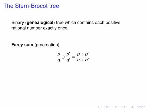
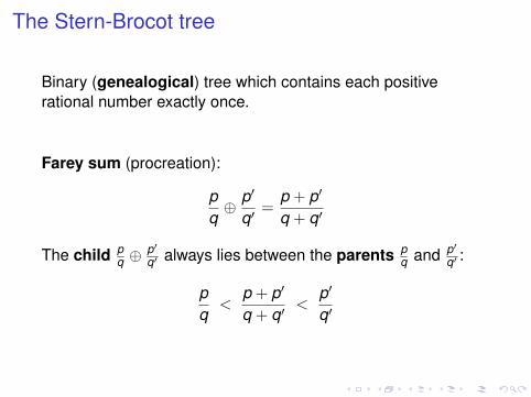
Binary (genealogical) tree which contains each positiverational number exactly once.
Farey sum (procreation):
pq⊕ p′
q′=
p + p′
q + q′
The child pq ⊕
p′q′ always lies between the parents p
q and p′q′ :
pq
<p + p′
q + q′<
p′
q′
The Stern-Brocot tree
Binary (genealogical) tree which contains each positiverational number exactly once.
Farey sum (procreation):
pq⊕ p′
q′=
p + p′
q + q′
The child pq ⊕
p′q′ always lies between the parents p
q and p′q′ :
pq
<p + p′
q + q′<
p′
q′
The Stern-Brocot tree
Binary (genealogical) tree which contains each positiverational number exactly once.
Farey sum (procreation):
pq⊕ p′
q′=
p + p′
q + q′
The child pq ⊕
p′q′ always lies between the parents p
q and p′q′ :
pq
<p + p′
q + q′<
p′
q′
The Stern-Brocot tree
Binary (genealogical) tree which contains each positiverational number exactly once.
Farey sum (procreation):
pq⊕ p′
q′=
p + p′
q + q′
The child pq ⊕
p′q′ always lies between the parents p
q and p′q′ :
pq
<p + p′
q + q′<
p′
q′
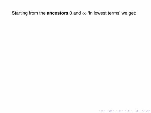
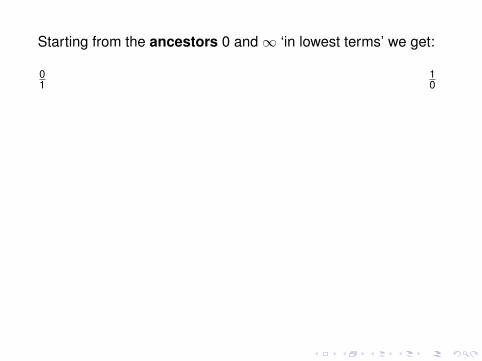
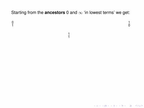
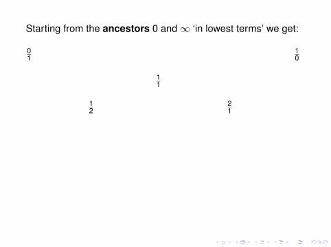
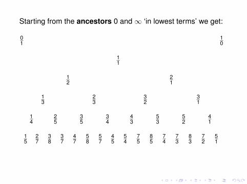
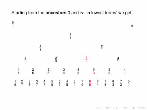
Starting from the ancestors 0 and ∞ ‘in lowest terms’ we get:
01
10
11
12
21
13
23
32
31
14
25
35
34
43
53
52
41
15
27
38
37
47
58
57
45
54
75
85
74
73
83
72
51
Starting from the ancestors 0 and ∞ ‘in lowest terms’ we get:
01
10
11
12
21
13
23
32
31
14
25
35
34
43
53
52
41
15
27
38
37
47
58
57
45
54
75
85
74
73
83
72
51
Starting from the ancestors 0 and ∞ ‘in lowest terms’ we get:
01
10
11
12
21
13
23
32
31
14
25
35
34
43
53
52
41
15
27
38
37
47
58
57
45
54
75
85
74
73
83
72
51
Starting from the ancestors 0 and ∞ ‘in lowest terms’ we get:
01
10
11
12
21
13
23
32
31
14
25
35
34
43
53
52
41
15
27
38
37
47
58
57
45
54
75
85
74
73
83
72
51

Starting from the ancestors 0 and ∞ ‘in lowest terms’ we get:
01
10
11
12
21
13
23
32
31
14
25
35
34
43
53
52
41
15
27
38
37
47
58
57
45
54
75
85
74
73
83
72
51

Starting from the ancestors 0 and ∞ ‘in lowest terms’ we get:
01
10
11
12
21
13
23
32
31
14
25
35
34
43
53
52
41
15
27
38
37
47
58
57
45
54
75
85
74
73
83
72
51
Starting from the ancestors 0 and ∞ ‘in lowest terms’ we get:
01
10
11
12
21
13
23
32
31
14
25
35
34
43
53
52
41
15
27
38
37
47
58
57
45
54
75
85
74
73
83
72
51
Starting from the ancestors 0 and ∞ ‘in lowest terms’ we get:
01
10
11
12
21
13
23
32
31
14
25
35
34
43
53
52
41
15
27
38
37
47
58
57
45
54
75
85
74
73
83
72
51
CONNECTION TO CONTINUED FRACTIONS
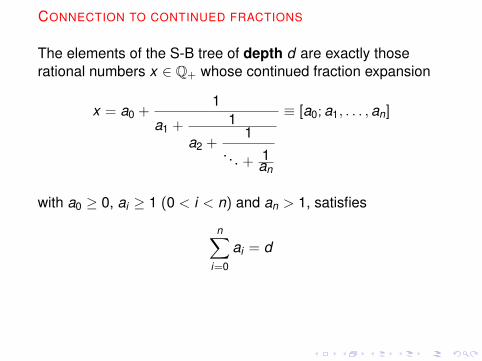
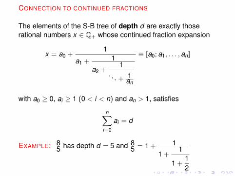
The elements of the S-B tree of depth d are exactly thoserational numbers x ∈ Q+ whose continued fraction expansion
x = a0 +1
a1 + 1
a2 +1
. . . + 1an
≡ [a0; a1, . . . , an]
with a0 ≥ 0, ai ≥ 1 (0 < i < n) and an > 1, satisfies
n∑i=0
ai = d
EXAMPLE: 85 has depth d = 5 and 8
5 = 1 + 1
1 +1
1 +12
CONNECTION TO CONTINUED FRACTIONS
The elements of the S-B tree of depth d are exactly thoserational numbers x ∈ Q+ whose continued fraction expansion
x = a0 +1
a1 + 1
a2 +1
. . . + 1an
≡ [a0; a1, . . . , an]
with a0 ≥ 0, ai ≥ 1 (0 < i < n) and an > 1, satisfies
n∑i=0
ai = d
EXAMPLE: 85 has depth d = 5 and 8
5 = 1 + 1
1 +1
1 +12
THE SLOW CONTINUED FRACTION ALGORITHM
Given x ∈ R+ there is a unique sequence {xk}k≥1 on the tree,which starts with x1 = 1 and converges to x , finite if x ∈ Q+,infinite otherwise:
if x = [a0; a1, a2, . . . ]
andp−2 = 0, p−1 = 1, pn = an pn−1 + pn−2
q−2 = 1, q−1 = 0, qn = an qn−1 + qn−2
then xk = k if k ≤ a0 + 1, and for k > a0 + 1
xk =r pn−1 + pn−2
r qn−1 + qn−2, k =
n−1∑i=0
ai + r , 1 ≤ r ≤ an
=⇒ xk is called a Farey convergent (FC) of x . If r = an thenxk = pn/qn = [a0; a1, a2, . . . , an−1, an] is the usual continuedfraction convergent (CFC) of x .
THE SLOW CONTINUED FRACTION ALGORITHM
Given x ∈ R+ there is a unique sequence {xk}k≥1 on the tree,which starts with x1 = 1 and converges to x ,
finite if x ∈ Q+,infinite otherwise:
if x = [a0; a1, a2, . . . ]
andp−2 = 0, p−1 = 1, pn = an pn−1 + pn−2
q−2 = 1, q−1 = 0, qn = an qn−1 + qn−2
then xk = k if k ≤ a0 + 1, and for k > a0 + 1
xk =r pn−1 + pn−2
r qn−1 + qn−2, k =
n−1∑i=0
ai + r , 1 ≤ r ≤ an
=⇒ xk is called a Farey convergent (FC) of x . If r = an thenxk = pn/qn = [a0; a1, a2, . . . , an−1, an] is the usual continuedfraction convergent (CFC) of x .
THE SLOW CONTINUED FRACTION ALGORITHM
Given x ∈ R+ there is a unique sequence {xk}k≥1 on the tree,which starts with x1 = 1 and converges to x , finite if x ∈ Q+,infinite otherwise:
if x = [a0; a1, a2, . . . ]
andp−2 = 0, p−1 = 1, pn = an pn−1 + pn−2
q−2 = 1, q−1 = 0, qn = an qn−1 + qn−2
then xk = k if k ≤ a0 + 1, and for k > a0 + 1
xk =r pn−1 + pn−2
r qn−1 + qn−2, k =
n−1∑i=0
ai + r , 1 ≤ r ≤ an
=⇒ xk is called a Farey convergent (FC) of x . If r = an thenxk = pn/qn = [a0; a1, a2, . . . , an−1, an] is the usual continuedfraction convergent (CFC) of x .
THE SLOW CONTINUED FRACTION ALGORITHM
Given x ∈ R+ there is a unique sequence {xk}k≥1 on the tree,which starts with x1 = 1 and converges to x , finite if x ∈ Q+,infinite otherwise:
if x = [a0; a1, a2, . . . ]
andp−2 = 0, p−1 = 1, pn = an pn−1 + pn−2
q−2 = 1, q−1 = 0, qn = an qn−1 + qn−2
then xk = k if k ≤ a0 + 1, and for k > a0 + 1
xk =r pn−1 + pn−2
r qn−1 + qn−2, k =
n−1∑i=0
ai + r , 1 ≤ r ≤ an
=⇒ xk is called a Farey convergent (FC) of x .
If r = an thenxk = pn/qn = [a0; a1, a2, . . . , an−1, an] is the usual continuedfraction convergent (CFC) of x .
THE SLOW CONTINUED FRACTION ALGORITHM
Given x ∈ R+ there is a unique sequence {xk}k≥1 on the tree,which starts with x1 = 1 and converges to x , finite if x ∈ Q+,infinite otherwise:
if x = [a0; a1, a2, . . . ]
andp−2 = 0, p−1 = 1, pn = an pn−1 + pn−2
q−2 = 1, q−1 = 0, qn = an qn−1 + qn−2
then xk = k if k ≤ a0 + 1, and for k > a0 + 1
xk =r pn−1 + pn−2
r qn−1 + qn−2, k =
n−1∑i=0
ai + r , 1 ≤ r ≤ an
=⇒ xk is called a Farey convergent (FC) of x . If r = an thenxk = pn/qn = [a0; a1, a2, . . . , an−1, an] is the usual continuedfraction convergent (CFC) of x .
GROWTH OF THE DENOMINATORS
For x ∈ (0, 1) the CFC’s denominators qn typically growexponentially fast:
log qn
n→ π2
12 log 2almost everywhere
Write a FC as xk = tk/sk (note that min{sk} = k andmax{sk} = fk , the k−th Fibonacci number).If k =
∑ni=1 ai + r then qn−1 < sk ≤ qn.
Moreover (Khinchin and Lévy):
1n log n
n∑i=1
ai →1
log 2in measure
Thereforelog sk
k∼ π2
12 log kin measure
GROWTH OF THE DENOMINATORS
For x ∈ (0, 1) the CFC’s denominators qn typically growexponentially fast:
log qn
n→ π2
12 log 2almost everywhere
Write a FC as xk = tk/sk (note that min{sk} = k andmax{sk} = fk , the k−th Fibonacci number).
If k =∑n
i=1 ai + r then qn−1 < sk ≤ qn.Moreover (Khinchin and Lévy):
1n log n
n∑i=1
ai →1
log 2in measure
Thereforelog sk
k∼ π2
12 log kin measure
GROWTH OF THE DENOMINATORS
For x ∈ (0, 1) the CFC’s denominators qn typically growexponentially fast:
log qn
n→ π2
12 log 2almost everywhere
Write a FC as xk = tk/sk (note that min{sk} = k andmax{sk} = fk , the k−th Fibonacci number).If k =
∑ni=1 ai + r then qn−1 < sk ≤ qn.
Moreover (Khinchin and Lévy):
1n log n
n∑i=1
ai →1
log 2in measure
Thereforelog sk
k∼ π2
12 log kin measure
GROWTH OF THE DENOMINATORS
For x ∈ (0, 1) the CFC’s denominators qn typically growexponentially fast:
log qn
n→ π2
12 log 2almost everywhere
Write a FC as xk = tk/sk (note that min{sk} = k andmax{sk} = fk , the k−th Fibonacci number).If k =
∑ni=1 ai + r then qn−1 < sk ≤ qn.
Moreover (Khinchin and Lévy):
1n log n
n∑i=1
ai →1
log 2in measure
Thereforelog sk
k∼ π2
12 log kin measure
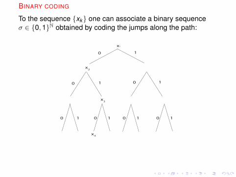
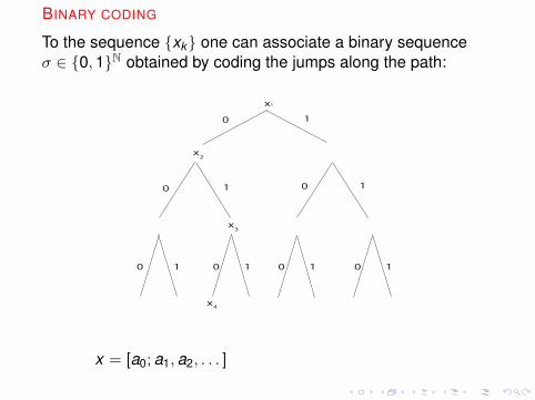
BINARY CODING
To the sequence {xk} one can associate a binary sequenceσ ∈ {0, 1}N obtained by coding the jumps along the path:
0 1
0 1 0 1
0 1 0 1 0 1 0 1
x2
x3
x4
x1
x = [a0; a1, a2, . . . ] ⇐⇒ σ(x) = 1a00a11a2 . . .
BINARY CODING
To the sequence {xk} one can associate a binary sequenceσ ∈ {0, 1}N obtained by coding the jumps along the path:
0 1
0 1 0 1
0 1 0 1 0 1 0 1
x2
x3
x4
x1
x = [a0; a1, a2, . . . ] ⇐⇒ σ(x) = 1a00a11a2 . . .
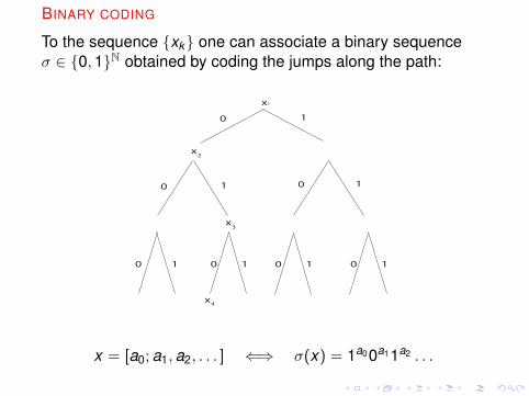
BINARY CODING
To the sequence {xk} one can associate a binary sequenceσ ∈ {0, 1}N obtained by coding the jumps along the path:
0 1
0 1 0 1
0 1 0 1 0 1 0 1
x2
x3
x4
x1
x = [a0; a1, a2, . . . ]
⇐⇒ σ(x) = 1a00a11a2 . . .
BINARY CODING
To the sequence {xk} one can associate a binary sequenceσ ∈ {0, 1}N obtained by coding the jumps along the path:
0 1
0 1 0 1
0 1 0 1 0 1 0 1
x2
x3
x4
x1
x = [a0; a1, a2, . . . ] ⇐⇒ σ(x) = 1a00a11a2 . . .
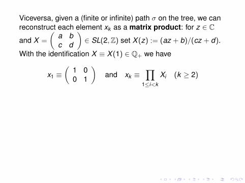
Viceversa, given a (finite or infinite) path σ on the tree, we canreconstruct each element xk as a matrix product:
for z ∈ C
and X =
(a bc d
)∈ SL(2, Z) set X (z) := (az + b)/(cz + d).
With the identification X ≡ X (1) ∈ Q+ we have
x1 ≡(
1 00 1
)and xk ≡
∏1≤i<k
Xi (k ≥ 2)
where
Xi =
{A , if σi = 0B , if σi = 1
A =
(1 01 1
)e B =
(1 10 1
)
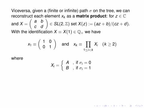
Viceversa, given a (finite or infinite) path σ on the tree, we canreconstruct each element xk as a matrix product: for z ∈ C
and X =
(a bc d
)∈ SL(2, Z) set X (z) := (az + b)/(cz + d).
With the identification X ≡ X (1) ∈ Q+ we have
x1 ≡(
1 00 1
)and xk ≡
∏1≤i<k
Xi (k ≥ 2)
where
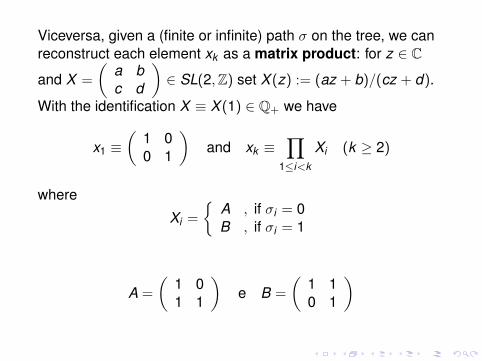
Xi =
{A , if σi = 0B , if σi = 1
A =
(1 01 1
)e B =
(1 10 1
)
Viceversa, given a (finite or infinite) path σ on the tree, we canreconstruct each element xk as a matrix product: for z ∈ C
and X =
(a bc d
)∈ SL(2, Z) set X (z) := (az + b)/(cz + d).
With the identification X ≡ X (1) ∈ Q+ we have
x1 ≡(
1 00 1
)and xk ≡
∏1≤i<k
Xi (k ≥ 2)
where
Xi =
{A , if σi = 0B , if σi = 1
A =
(1 01 1
)e B =
(1 10 1
)
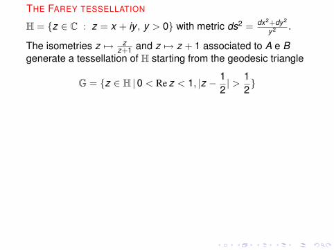
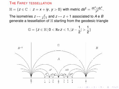
THE FAREY TESSELLATION
H = {z ∈ C : z = x + iy , y > 0} with metric ds2 = dx2+dy2
y2 .
The isometries z 7→ zz+1 and z 7→ z + 1 associated to A e B
generate a tessellation of H starting from the geodesic triangle
G = {z ∈ H |0 < Re z < 1, |z − 12| > 1
2}
THE FAREY TESSELLATION
H = {z ∈ C : z = x + iy , y > 0} with metric ds2 = dx2+dy2
y2 .
The isometries z 7→ zz+1 and z 7→ z + 1 associated to A e B
generate a tessellation of H starting from the geodesic triangle
G = {z ∈ H |0 < Re z < 1, |z − 12| > 1
2}
THE FAREY TESSELLATION
H = {z ∈ C : z = x + iy , y > 0} with metric ds2 = dx2+dy2
y2 .
The isometries z 7→ zz+1 and z 7→ z + 1 associated to A e B
generate a tessellation of H starting from the geodesic triangle
G = {z ∈ H |0 < Re z < 1, |z − 12| > 1
2}
THE FAREY TESSELLATION
H = {z ∈ C : z = x + iy , y > 0} with metric ds2 = dx2+dy2
y2 .
The isometries z 7→ zz+1 and z 7→ z + 1 associated to A e B
generate a tessellation of H starting from the geodesic triangle
G = {z ∈ H |0 < Re z < 1, |z − 12| > 1
2}
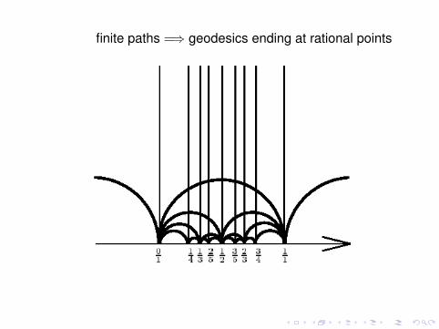
finite paths =⇒ geodesics ending at rational points
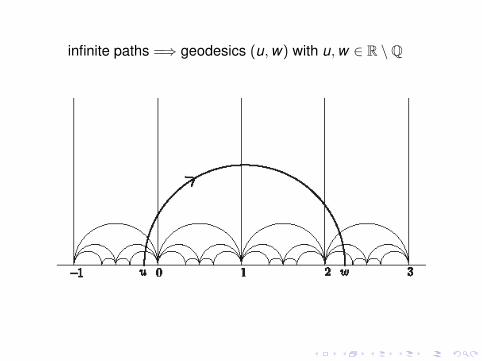
infinite paths =⇒ geodesics (u, w) with u, w ∈ R \Q
THE PERMUTED S-B TREE
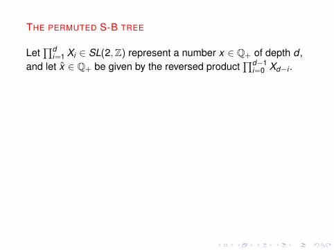
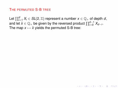
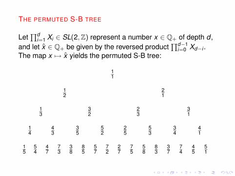
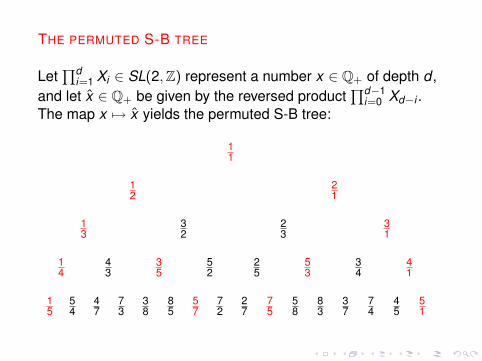
Let∏d
i=1 Xi ∈ SL(2, Z) represent a number x ∈ Q+ of depth d ,and let x̂ ∈ Q+ be given by the reversed product
∏d−1i=0 Xd−i .
The map x 7→ x̂ yields the permuted S-B tree:
11
12
21
13
32
23
31
14
43
35
52
25
53
34
41
15
54
47
73
38
85
57
72
27
75
58
83
37
74
45
51
THE PERMUTED S-B TREE
Let∏d
i=1 Xi ∈ SL(2, Z) represent a number x ∈ Q+ of depth d ,
and let x̂ ∈ Q+ be given by the reversed product∏d−1
i=0 Xd−i .The map x 7→ x̂ yields the permuted S-B tree:
11
12
21
13
32
23
31
14
43
35
52
25
53
34
41
15
54
47
73
38
85
57
72
27
75
58
83
37
74
45
51
THE PERMUTED S-B TREE
Let∏d
i=1 Xi ∈ SL(2, Z) represent a number x ∈ Q+ of depth d ,and
let x̂ ∈ Q+ be given by the reversed product∏d−1
i=0 Xd−i .The map x 7→ x̂ yields the permuted S-B tree:
11
12
21
13
32
23
31
14
43
35
52
25
53
34
41
15
54
47
73
38
85
57
72
27
75
58
83
37
74
45
51
THE PERMUTED S-B TREE
Let∏d
i=1 Xi ∈ SL(2, Z) represent a number x ∈ Q+ of depth d ,and let x̂ ∈ Q+ be given by the reversed product
∏d−1i=0 Xd−i .
The map x 7→ x̂ yields the permuted S-B tree:
11
12
21
13
32
23
31
14
43
35
52
25
53
34
41
15
54
47
73
38
85
57
72
27
75
58
83
37
74
45
51
THE PERMUTED S-B TREE
Let∏d
i=1 Xi ∈ SL(2, Z) represent a number x ∈ Q+ of depth d ,and let x̂ ∈ Q+ be given by the reversed product
∏d−1i=0 Xd−i .
The map x 7→ x̂ yields the permuted S-B tree:
11
12
21
13
32
23
31
14
43
35
52
25
53
34
41
15
54
47
73
38
85
57
72
27
75
58
83
37
74
45
51
THE PERMUTED S-B TREE
Let∏d
i=1 Xi ∈ SL(2, Z) represent a number x ∈ Q+ of depth d ,and let x̂ ∈ Q+ be given by the reversed product
∏d−1i=0 Xd−i .
The map x 7→ x̂ yields the permuted S-B tree:
11
12
21
13
32
23
31
14
43
35
52
25
53
34
41
15
54
47
73
38
85
57
72
27
75
58
83
37
74
45
51
THE PERMUTED S-B TREE
Let∏d
i=1 Xi ∈ SL(2, Z) represent a number x ∈ Q+ of depth d ,and let x̂ ∈ Q+ be given by the reversed product
∏d−1i=0 Xd−i .
The map x 7→ x̂ yields the permuted S-B tree:
11
12
21
13
32
23
31
14
43
35
52
25
53
34
41
15
54
47
73
38
85
57
72
27
75
58
83
37
74
45
51
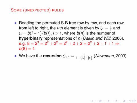
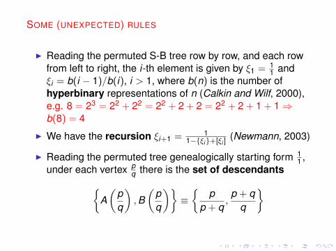
SOME (UNEXPECTED) RULES
I Reading the permuted S-B tree row by row, and each rowfrom left to right, the i-th element is given by ξ1 = 1
1 andξi = b(i − 1)/b(i), i > 1, where b(n) is the number ofhyperbinary representations of n (Calkin and Wilf, 2000),e.g. 8 = 23 = 22 + 22 = 22 + 2 + 2 = 22 + 2 + 1 + 1 ⇒b(8) = 4
I We have the recursion ξi+1 = 11−{ξi}+[ξi ]
(Newmann, 2003)
I Reading the permuted tree genealogically starting form 11 ,
under each vertex pq there is the set of descendants{
A(
pq
), B(
pq
)}≡{
pp + q
,p + q
q
}
SOME (UNEXPECTED) RULES
I Reading the permuted S-B tree row by row, and each rowfrom left to right, the i-th element is given by ξ1 = 1
1 andξi = b(i − 1)/b(i), i > 1,
where b(n) is the number ofhyperbinary representations of n (Calkin and Wilf, 2000),e.g. 8 = 23 = 22 + 22 = 22 + 2 + 2 = 22 + 2 + 1 + 1 ⇒b(8) = 4
I We have the recursion ξi+1 = 11−{ξi}+[ξi ]
(Newmann, 2003)
I Reading the permuted tree genealogically starting form 11 ,
under each vertex pq there is the set of descendants{
A(
pq
), B(
pq
)}≡{
pp + q
,p + q
q
}
SOME (UNEXPECTED) RULES
I Reading the permuted S-B tree row by row, and each rowfrom left to right, the i-th element is given by ξ1 = 1
1 andξi = b(i − 1)/b(i), i > 1, where b(n) is the number ofhyperbinary representations of n (Calkin and Wilf, 2000),
e.g. 8 = 23 = 22 + 22 = 22 + 2 + 2 = 22 + 2 + 1 + 1 ⇒b(8) = 4
I We have the recursion ξi+1 = 11−{ξi}+[ξi ]
(Newmann, 2003)
I Reading the permuted tree genealogically starting form 11 ,
under each vertex pq there is the set of descendants{
A(
pq
), B(
pq
)}≡{
pp + q
,p + q
q
}
SOME (UNEXPECTED) RULES
I Reading the permuted S-B tree row by row, and each rowfrom left to right, the i-th element is given by ξ1 = 1
1 andξi = b(i − 1)/b(i), i > 1, where b(n) is the number ofhyperbinary representations of n (Calkin and Wilf, 2000),e.g. 8 = 23 = 22 + 22 = 22 + 2 + 2 = 22 + 2 + 1 + 1 ⇒b(8) = 4
I We have the recursion ξi+1 = 11−{ξi}+[ξi ]
(Newmann, 2003)
I Reading the permuted tree genealogically starting form 11 ,
under each vertex pq there is the set of descendants{
A(
pq
), B(
pq
)}≡{
pp + q
,p + q
q
}
SOME (UNEXPECTED) RULES
I Reading the permuted S-B tree row by row, and each rowfrom left to right, the i-th element is given by ξ1 = 1
1 andξi = b(i − 1)/b(i), i > 1, where b(n) is the number ofhyperbinary representations of n (Calkin and Wilf, 2000),e.g. 8 = 23 = 22 + 22 = 22 + 2 + 2 = 22 + 2 + 1 + 1 ⇒b(8) = 4
I We have the recursion ξi+1 = 11−{ξi}+[ξi ]
(Newmann, 2003)
I Reading the permuted tree genealogically starting form 11 ,
under each vertex pq there is the set of descendants{
A(
pq
), B(
pq
)}≡{
pp + q
,p + q
q
}
Statistical mechanics
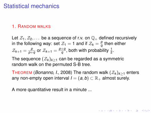
1. RANDOM WALKS
Let Z1,Z2, . . . be a sequence of r.v. on Q+ defined recursivelyin the following way: set Z1 = 1 and if Zk = p
q then eitherZk+1 = p
p+q or Zk+1 = p+qq , both with probability 1
2 .
The sequence (Zk )k≥1 can be regarded as a symmetricrandom walk on the permuted S-B tree.
THEOREM (Bonanno, I., 2008) The random walk (Zk )k≥1 entersany non-empty open interval I = (a, b) ⊂ R+ almost surely.
A more quantitative result in a minute ...
Statistical mechanics
1. RANDOM WALKS
Let Z1,Z2, . . . be a sequence of r.v. on Q+ defined recursivelyin the following way:
set Z1 = 1 and if Zk = pq then either
Zk+1 = pp+q or Zk+1 = p+q
q , both with probability 12 .
The sequence (Zk )k≥1 can be regarded as a symmetricrandom walk on the permuted S-B tree.
THEOREM (Bonanno, I., 2008) The random walk (Zk )k≥1 entersany non-empty open interval I = (a, b) ⊂ R+ almost surely.
A more quantitative result in a minute ...
Statistical mechanics
1. RANDOM WALKS
Let Z1,Z2, . . . be a sequence of r.v. on Q+ defined recursivelyin the following way: set Z1 = 1 and if Zk = p
q then eitherZk+1 = p
p+q or Zk+1 = p+qq , both with probability 1
2 .
The sequence (Zk )k≥1 can be regarded as a symmetricrandom walk on the permuted S-B tree.
THEOREM (Bonanno, I., 2008) The random walk (Zk )k≥1 entersany non-empty open interval I = (a, b) ⊂ R+ almost surely.
A more quantitative result in a minute ...
Statistical mechanics
1. RANDOM WALKS
Let Z1,Z2, . . . be a sequence of r.v. on Q+ defined recursivelyin the following way: set Z1 = 1 and if Zk = p
q then eitherZk+1 = p
p+q or Zk+1 = p+qq , both with probability 1
2 .
The sequence (Zk )k≥1 can be regarded as a symmetricrandom walk on the permuted S-B tree.
THEOREM (Bonanno, I., 2008) The random walk (Zk )k≥1 entersany non-empty open interval I = (a, b) ⊂ R+ almost surely.
A more quantitative result in a minute ...
2. KNAUF’ SPIN CHAIN
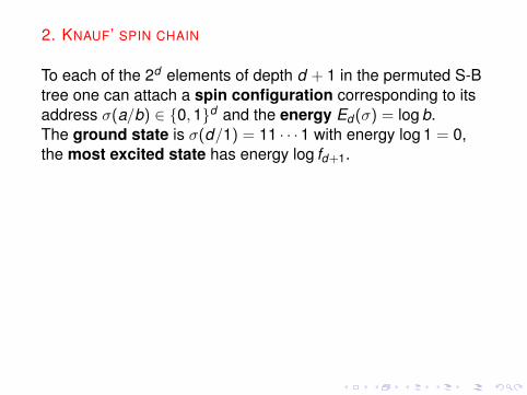
To each of the 2d elements of depth d + 1 in the permuted S-Btree one can attach a spin configuration corresponding to itsaddress σ(a/b) ∈ {0, 1}d and the energy Ed(σ) = log b.The ground state is σ(d/1) = 11 · · ·1 with energy log 1 = 0,the most excited state has energy log fd+1.The (canonical) partition function is
Zd(β) =∑
depth( ab )=d+1
b−β
The resulting interaction is ferromagnetic (Knauf, 1993):
jd(τ) := − 12d
∑σ∈{0,1}d
Ed(σ) · (−1)σ·τ ≥ 0 , τ ∈ {0, 1}d \ 0d
2. KNAUF’ SPIN CHAIN
To each of the 2d elements of depth d + 1 in the permuted S-Btree one can attach a spin configuration corresponding to itsaddress σ(a/b) ∈ {0, 1}d and the energy Ed(σ) = log b.
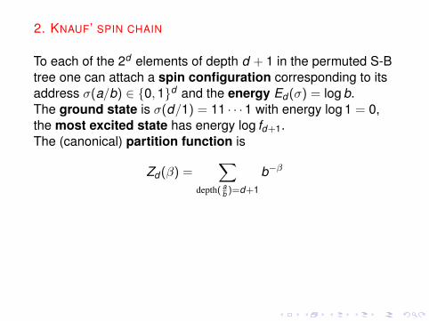
The ground state is σ(d/1) = 11 · · ·1 with energy log 1 = 0,the most excited state has energy log fd+1.The (canonical) partition function is
Zd(β) =∑
depth( ab )=d+1
b−β
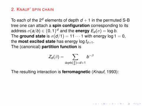
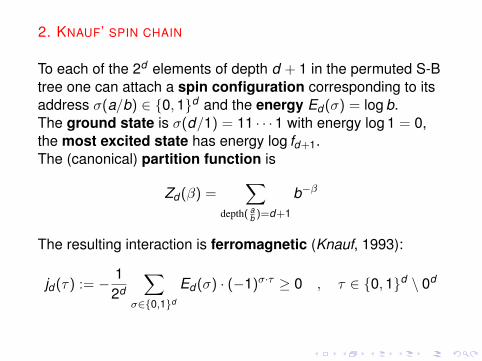
The resulting interaction is ferromagnetic (Knauf, 1993):
jd(τ) := − 12d
∑σ∈{0,1}d
Ed(σ) · (−1)σ·τ ≥ 0 , τ ∈ {0, 1}d \ 0d
2. KNAUF’ SPIN CHAIN
To each of the 2d elements of depth d + 1 in the permuted S-Btree one can attach a spin configuration corresponding to itsaddress σ(a/b) ∈ {0, 1}d and the energy Ed(σ) = log b.The ground state is σ(d/1) = 11 · · ·1 with energy log 1 = 0,
the most excited state has energy log fd+1.The (canonical) partition function is
Zd(β) =∑
depth( ab )=d+1
b−β
The resulting interaction is ferromagnetic (Knauf, 1993):
jd(τ) := − 12d
∑σ∈{0,1}d
Ed(σ) · (−1)σ·τ ≥ 0 , τ ∈ {0, 1}d \ 0d
2. KNAUF’ SPIN CHAIN
To each of the 2d elements of depth d + 1 in the permuted S-Btree one can attach a spin configuration corresponding to itsaddress σ(a/b) ∈ {0, 1}d and the energy Ed(σ) = log b.The ground state is σ(d/1) = 11 · · ·1 with energy log 1 = 0,the most excited state has energy log fd+1.
The (canonical) partition function is
Zd(β) =∑
depth( ab )=d+1
b−β
The resulting interaction is ferromagnetic (Knauf, 1993):
jd(τ) := − 12d
∑σ∈{0,1}d
Ed(σ) · (−1)σ·τ ≥ 0 , τ ∈ {0, 1}d \ 0d
2. KNAUF’ SPIN CHAIN
To each of the 2d elements of depth d + 1 in the permuted S-Btree one can attach a spin configuration corresponding to itsaddress σ(a/b) ∈ {0, 1}d and the energy Ed(σ) = log b.The ground state is σ(d/1) = 11 · · ·1 with energy log 1 = 0,the most excited state has energy log fd+1.The (canonical) partition function is
Zd(β) =∑
depth( ab )=d+1
b−β
The resulting interaction is ferromagnetic (Knauf, 1993):
jd(τ) := − 12d
∑σ∈{0,1}d
Ed(σ) · (−1)σ·τ ≥ 0 , τ ∈ {0, 1}d \ 0d
2. KNAUF’ SPIN CHAIN
To each of the 2d elements of depth d + 1 in the permuted S-Btree one can attach a spin configuration corresponding to itsaddress σ(a/b) ∈ {0, 1}d and the energy Ed(σ) = log b.The ground state is σ(d/1) = 11 · · ·1 with energy log 1 = 0,the most excited state has energy log fd+1.The (canonical) partition function is
Zd(β) =∑
depth( ab )=d+1
b−β
The resulting interaction is ferromagnetic (Knauf, 1993):
jd(τ) := − 12d
∑σ∈{0,1}d
Ed(σ) · (−1)σ·τ ≥ 0 , τ ∈ {0, 1}d \ 0d
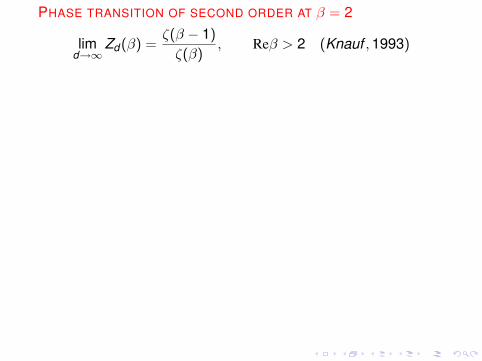
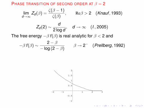
PHASE TRANSITION OF SECOND ORDER AT β = 2
limd→∞
Zd(β) =ζ(β − 1)
ζ(β), Reβ > 2 (Knauf , 1993)
Zd(2) ∼ d2 log d
, d →∞ (I., 2005)
The free energy −β f (β) is real analytic for β < 2 and
−β f (β) ∼ 2− β
− log (2− β)β → 2− (Prellberg, 1992)
-2 -1 1 2 3
-1
-0.5
0.5
1
1.5
2
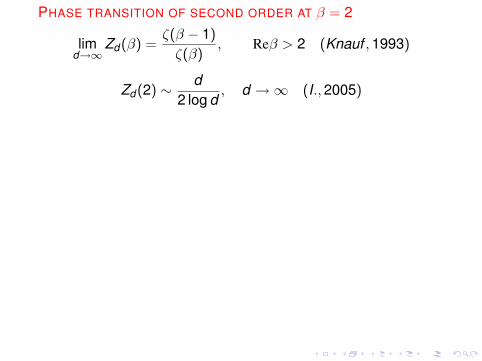
PHASE TRANSITION OF SECOND ORDER AT β = 2
limd→∞
Zd(β) =ζ(β − 1)
ζ(β), Reβ > 2 (Knauf , 1993)
Zd(2) ∼ d2 log d
, d →∞ (I., 2005)
The free energy −β f (β) is real analytic for β < 2 and
−β f (β) ∼ 2− β
− log (2− β)β → 2− (Prellberg, 1992)
-2 -1 1 2 3
-1
-0.5
0.5
1
1.5
2
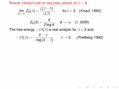
PHASE TRANSITION OF SECOND ORDER AT β = 2
limd→∞
Zd(β) =ζ(β − 1)
ζ(β), Reβ > 2 (Knauf , 1993)
Zd(2) ∼ d2 log d
, d →∞ (I., 2005)
The free energy −β f (β) is real analytic for β < 2 and
−β f (β) ∼ 2− β
− log (2− β)β → 2− (Prellberg, 1992)
-2 -1 1 2 3
-1
-0.5
0.5
1
1.5
2
PHASE TRANSITION OF SECOND ORDER AT β = 2
limd→∞
Zd(β) =ζ(β − 1)
ζ(β), Reβ > 2 (Knauf , 1993)
Zd(2) ∼ d2 log d
, d →∞ (I., 2005)
The free energy −β f (β) is real analytic for β < 2 and
−β f (β) ∼ 2− β
− log (2− β)β → 2− (Prellberg, 1992)
-2 -1 1 2 3
-1
-0.5
0.5
1
1.5
2
PHASE TRANSITION OF SECOND ORDER AT β = 2
limd→∞
Zd(β) =ζ(β − 1)
ζ(β), Reβ > 2 (Knauf , 1993)
Zd(2) ∼ d2 log d
, d →∞ (I., 2005)
The free energy −β f (β) is real analytic for β < 2 and
−β f (β) ∼ 2− β
− log (2− β)β → 2− (Prellberg, 1992)
-2 -1 1 2 3
-1
-0.5
0.5
1
1.5
2
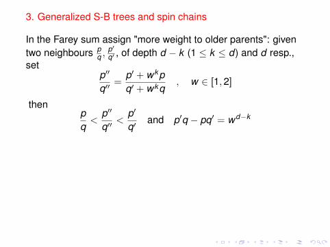
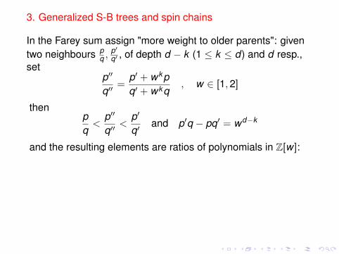
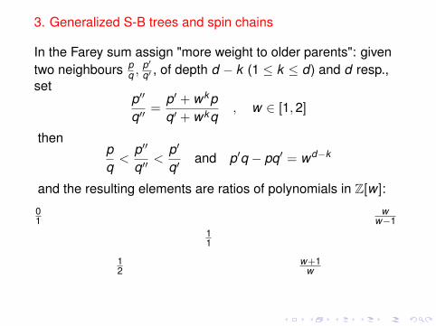
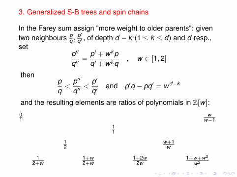
3. Generalized S-B trees and spin chains
In the Farey sum assign "more weight to older parents": giventwo neighbours p
q , p′q′ , of depth d − k (1 ≤ k ≤ d) and d resp.,
setp′′
q′′=
p′ + wkpq′ + wkq
, w ∈ [1, 2]
thenpq
<p′′
q′′<
p′
q′and p′q − pq′ = wd−k
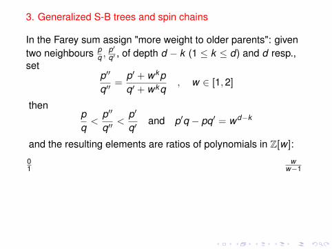
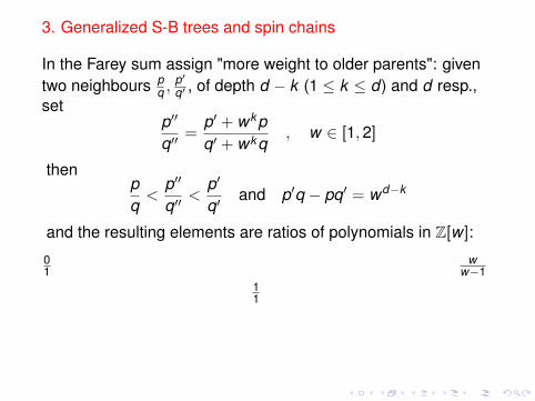
and the resulting elements are ratios of polynomials in Z[w ]:
01
ww−1
11
12
w+1w
12+w
1+w2+w
1+2w2w
1+w+w2
w2
3. Generalized S-B trees and spin chains
In the Farey sum assign "more weight to older parents":
giventwo neighbours p
q , p′q′ , of depth d − k (1 ≤ k ≤ d) and d resp.,
setp′′
q′′=
p′ + wkpq′ + wkq
, w ∈ [1, 2]
thenpq
<p′′
q′′<
p′
q′and p′q − pq′ = wd−k
and the resulting elements are ratios of polynomials in Z[w ]:
01
ww−1
11
12
w+1w
12+w
1+w2+w
1+2w2w
1+w+w2
w2
3. Generalized S-B trees and spin chains
In the Farey sum assign "more weight to older parents": giventwo neighbours p
q , p′q′ , of depth d − k (1 ≤ k ≤ d) and d resp.,
setp′′
q′′=
p′ + wkpq′ + wkq
, w ∈ [1, 2]
thenpq
<p′′
q′′<
p′
q′and p′q − pq′ = wd−k
and the resulting elements are ratios of polynomials in Z[w ]:
01
ww−1
11
12
w+1w
12+w
1+w2+w
1+2w2w
1+w+w2
w2
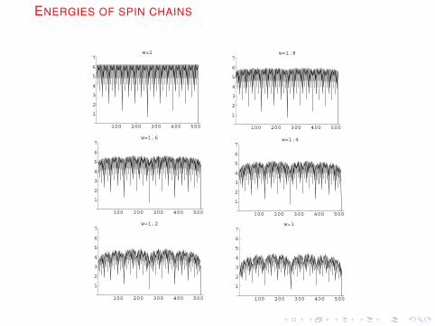
ENERGIES OF SPIN CHAINS
100 200 300 400 500
1
2
3
4
5
6
7w=2�
100 200 300 400 500
1
2
3
4
5
6
7w=1.8
100 200 300 400 500
1
2
3
4
5
6
7w=1.6�
100 200 300 400 500
1
2
3
4
5
6
7w=1.4�
100 200 300 400 500
1
2
3
4
5
6
7w=1.2�
100 200 300 400 500
1
2
3
4
5
6
7w=1�
ENERGIES OF SPIN CHAINS
100 200 300 400 500
1
2
3
4
5
6
7w=2�
100 200 300 400 500
1
2
3
4
5
6
7w=1.8
100 200 300 400 500
1
2
3
4
5
6
7w=1.6�
100 200 300 400 500
1
2
3
4
5
6
7w=1.4�
100 200 300 400 500
1
2
3
4
5
6
7w=1.2�
100 200 300 400 500
1
2
3
4
5
6
7w=1�
THEOREM (Degli Esposti, I., Knauf, 2007)
I The interaction of the spin chain is ferromagnetic for eachw ∈ [1, 2].
I There is a monotonically decreasing function βcr (w), withβcr (1) = 2 and βcr (2) = 1, such that the partition fct Zd(β)has a finite limit as d →∞ whenever β > βcr .
I For w = 1 the phase transition at βcr = 2 is of secondorder, but for 1 < w ≤ 2 the first derivative of −β f (β) isdiscontinuous at βcr (first order transition). Moreover, for allw ∈ [1, 2] the magnetization jumps at βcr from 1 to 0.

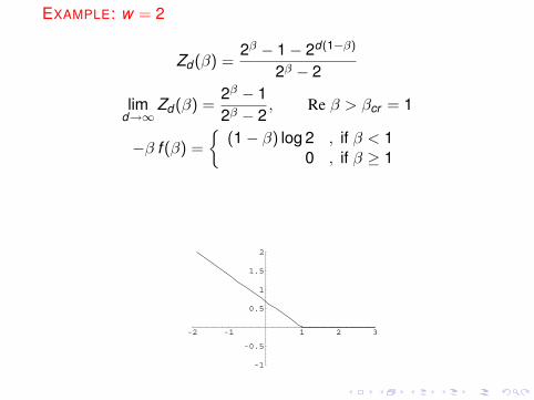
EXAMPLE: w = 2
Zd(β) =2β − 1− 2d(1−β)
2β − 2
limd→∞
Zd(β) =2β − 12β − 2
, Re β > βcr = 1
−β f (β) =
{(1− β) log 2 , if β < 1
0 , if β ≥ 1
-2 -1 1 2 3
-1
-0.5
0.5
1
1.5
2
EXAMPLE: w = 2
Zd(β) =2β − 1− 2d(1−β)
2β − 2
limd→∞
Zd(β) =2β − 12β − 2
, Re β > βcr = 1
−β f (β) =
{(1− β) log 2 , if β < 1
0 , if β ≥ 1
-2 -1 1 2 3
-1
-0.5
0.5
1
1.5
2

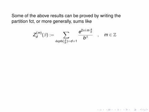
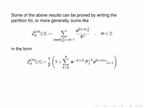
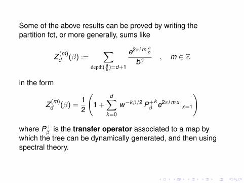
Some of the above results can be proved by writing thepartition fct, or more generally, sums like
Z (m)d (β) :=
∑depth( a
b )=d+1
e2πi m ab
bβ, m ∈ Z
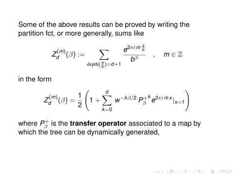
in the form
Z (m)d (β) =
12
(1 +
d∑k=0
w−kβ/2 P+β
ke2πi m x |x=1
)
where P+β is the transfer operator associated to a map by
which the tree can be dynamically generated, and then usingspectral theory.
Some of the above results can be proved by writing thepartition fct, or more generally, sums like
Z (m)d (β) :=
∑depth( a
b )=d+1
e2πi m ab
bβ, m ∈ Z
in the form
Z (m)d (β) =
12
(1 +
d∑k=0
w−kβ/2 P+β
ke2πi m x |x=1
)
where P+β is the transfer operator associated to a map by
which the tree can be dynamically generated,
and then usingspectral theory.
Some of the above results can be proved by writing thepartition fct, or more generally, sums like
Z (m)d (β) :=
∑depth( a
b )=d+1
e2πi m ab
bβ, m ∈ Z
in the form
Z (m)d (β) =
12
(1 +
d∑k=0
w−kβ/2 P+β
ke2πi m x |x=1
)
where P+β is the transfer operator associated to a map by
which the tree can be dynamically generated, and then usingspectral theory.
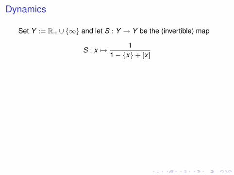
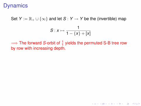
Dynamics
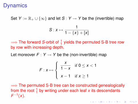
Set Y := R+ ∪ {∞} and let S : Y → Y be the (invertible) map
S : x 7→ 11− {x}+ [x ]
=⇒ The forward S-orbit of 11 yields the permuted S-B tree row
by row with increasing depth.
Let moreover F : Y → Y be the (non-invertible) map
F : x 7→
x
1− xif 0 ≤ x < 1
x − 1 if x ≥ 1
=⇒ The permuted S-B tree can be constructed genealogicallyfrom the root 1
1 by writing under each leaf x its descendantsF−1(x).
Dynamics
Set Y := R+ ∪ {∞} and let S : Y → Y be the (invertible) map
S : x 7→ 11− {x}+ [x ]
=⇒ The forward S-orbit of 11 yields the permuted S-B tree row
by row with increasing depth.
Let moreover F : Y → Y be the (non-invertible) map
F : x 7→
x
1− xif 0 ≤ x < 1
x − 1 if x ≥ 1
=⇒ The permuted S-B tree can be constructed genealogicallyfrom the root 1
1 by writing under each leaf x its descendantsF−1(x).
We plot the interval maps S̃ := φ ◦ S ◦ φ−1 and F̃ := φ ◦ F ◦ φ−1
where φ(x) := x/(1 + x) (maps the S-B tree to the Farey tree):
S̃(x) =1
2−{
x1−x
}+[
x1−x
] , F̃ =
x
1− xif 0 ≤ x < 1
2
2− 1x if 1
2 ≤ x ≤ 1
0.2 0.4 0.6 0.8 1
0.2
0.4
0.6
0.8
1
0.2 0.4 0.6 0.8 1
0.2
0.4
0.6
0.8
1
Figure:
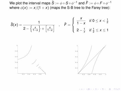
We plot the interval maps S̃ := φ ◦ S ◦ φ−1 and F̃ := φ ◦ F ◦ φ−1
where φ(x) := x/(1 + x) (maps the S-B tree to the Farey tree):
S̃(x) =1
2−{
x1−x
}+[
x1−x
] , F̃ =
x
1− xif 0 ≤ x < 1
2
2− 1x if 1
2 ≤ x ≤ 1
0.2 0.4 0.6 0.8 1
0.2
0.4
0.6
0.8
1
0.2 0.4 0.6 0.8 1
0.2
0.4
0.6
0.8
1
Figure:
CONJUGATIONS AND ERGODIC PROPERTIES
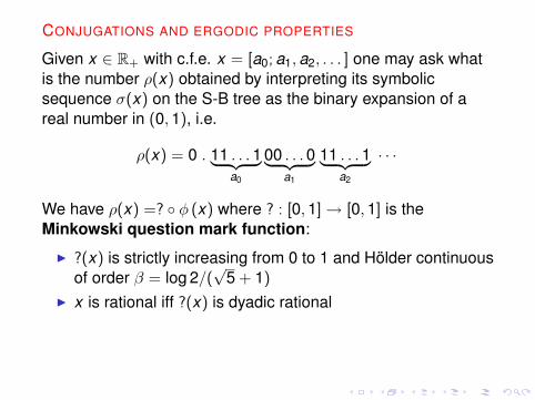
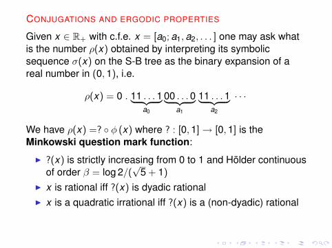
Given x ∈ R+ with c.f.e. x = [a0; a1, a2, . . . ] one may ask whatis the number ρ(x) obtained by interpreting its symbolicsequence σ(x) on the S-B tree as the binary expansion of areal number in (0, 1), i.e.
ρ(x) = 0 . 11 . . . 1︸ ︷︷ ︸a0
00 . . . 0︸ ︷︷ ︸a1
11 . . . 1︸ ︷︷ ︸a2
· · ·
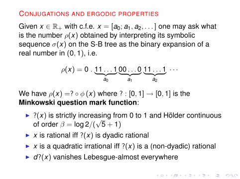
We have ρ(x) =? ◦ φ (x) where ? : [0, 1] → [0, 1] is theMinkowski question mark function:
I ?(x) is strictly increasing from 0 to 1 and Hölder continuousof order β = log 2/(
√5 + 1)
I x is rational iff ?(x) is dyadic rationalI x is a quadratic irrational iff ?(x) is a (non-dyadic) rationalI d?(x) vanishes Lebesgue-almost everywhere
CONJUGATIONS AND ERGODIC PROPERTIES
Given x ∈ R+ with c.f.e. x = [a0; a1, a2, . . . ] one may ask whatis the number ρ(x) obtained by interpreting its symbolicsequence σ(x) on the S-B tree as the binary expansion of areal number in (0, 1), i.e.
ρ(x) = 0 . 11 . . . 1︸ ︷︷ ︸a0
00 . . . 0︸ ︷︷ ︸a1
11 . . . 1︸ ︷︷ ︸a2
· · ·
We have ρ(x) =? ◦ φ (x) where ? : [0, 1] → [0, 1] is theMinkowski question mark function:
I ?(x) is strictly increasing from 0 to 1 and Hölder continuousof order β = log 2/(
√5 + 1)
I x is rational iff ?(x) is dyadic rational
I x is a quadratic irrational iff ?(x) is a (non-dyadic) rationalI d?(x) vanishes Lebesgue-almost everywhere
CONJUGATIONS AND ERGODIC PROPERTIES
Given x ∈ R+ with c.f.e. x = [a0; a1, a2, . . . ] one may ask whatis the number ρ(x) obtained by interpreting its symbolicsequence σ(x) on the S-B tree as the binary expansion of areal number in (0, 1), i.e.
ρ(x) = 0 . 11 . . . 1︸ ︷︷ ︸a0
00 . . . 0︸ ︷︷ ︸a1
11 . . . 1︸ ︷︷ ︸a2
· · ·
We have ρ(x) =? ◦ φ (x) where ? : [0, 1] → [0, 1] is theMinkowski question mark function:
I ?(x) is strictly increasing from 0 to 1 and Hölder continuousof order β = log 2/(
√5 + 1)
I x is rational iff ?(x) is dyadic rationalI x is a quadratic irrational iff ?(x) is a (non-dyadic) rational
I d?(x) vanishes Lebesgue-almost everywhere
CONJUGATIONS AND ERGODIC PROPERTIES
Given x ∈ R+ with c.f.e. x = [a0; a1, a2, . . . ] one may ask whatis the number ρ(x) obtained by interpreting its symbolicsequence σ(x) on the S-B tree as the binary expansion of areal number in (0, 1), i.e.
ρ(x) = 0 . 11 . . . 1︸ ︷︷ ︸a0
00 . . . 0︸ ︷︷ ︸a1
11 . . . 1︸ ︷︷ ︸a2
· · ·
We have ρ(x) =? ◦ φ (x) where ? : [0, 1] → [0, 1] is theMinkowski question mark function:
I ?(x) is strictly increasing from 0 to 1 and Hölder continuousof order β = log 2/(
√5 + 1)
I x is rational iff ?(x) is dyadic rationalI x is a quadratic irrational iff ?(x) is a (non-dyadic) rationalI d?(x) vanishes Lebesgue-almost everywhere
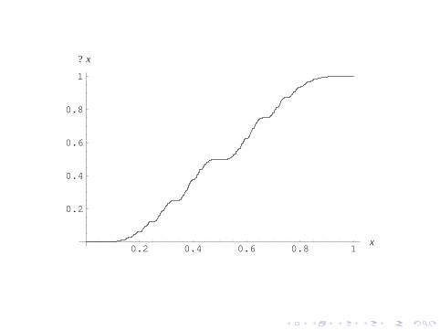
0.2 0.4 0.6 0.8 1x
0.2
0.4
0.6
0.8
1
?�x�
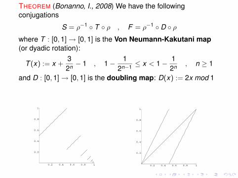
THEOREM (Bonanno, I., 2008) We have the followingconjugations
S = ρ−1 ◦ T ◦ ρ , F = ρ−1 ◦ D ◦ ρ
where T : [0, 1] → [0, 1] is the Von Neumann-Kakutani map(or dyadic rotation):
T (x) := x +32n − 1 , 1− 1
2n−1 ≤ x < 1− 12n , n ≥ 1
and D : [0, 1] → [0, 1] is the doubling map: D(x) := 2x mod 1
0.2 0.4 0.6 0.8 1
0.2
0.4
0.6
0.8
1
0.2 0.4 0.6 0.8 1
0.2
0.4
0.6
0.8
1
Figure:
Facts:
I both T and D preserve the Lebesgue measureI T is strictly ergodic, has rank one and discrete spectrumI T ◦ D = D ◦ T 2
Consequences:
I S preserves the singular measure dρ, is strictly ergodic,has rank one and discrete spectrum
I F preserves several measures. Among them: the measuredρ, which is the measure of maximal entropy (withentropy log 2), and the infinite a.c. measure dx/x (withzero entropy)
I the random walk (Zk )k≥1 enters the open intervalI = (a, b) ⊂ R+ with asymptotic frequency ρ(I)
I S ◦ F = F ◦ S2
Facts:
I both T and D preserve the Lebesgue measure
I T is strictly ergodic, has rank one and discrete spectrumI T ◦ D = D ◦ T 2
Consequences:
I S preserves the singular measure dρ, is strictly ergodic,has rank one and discrete spectrum
I F preserves several measures. Among them: the measuredρ, which is the measure of maximal entropy (withentropy log 2), and the infinite a.c. measure dx/x (withzero entropy)
I the random walk (Zk )k≥1 enters the open intervalI = (a, b) ⊂ R+ with asymptotic frequency ρ(I)
I S ◦ F = F ◦ S2
Facts:
I both T and D preserve the Lebesgue measureI T is strictly ergodic, has rank one and discrete spectrum
I T ◦ D = D ◦ T 2
Consequences:
I S preserves the singular measure dρ, is strictly ergodic,has rank one and discrete spectrum
I F preserves several measures. Among them: the measuredρ, which is the measure of maximal entropy (withentropy log 2), and the infinite a.c. measure dx/x (withzero entropy)
I the random walk (Zk )k≥1 enters the open intervalI = (a, b) ⊂ R+ with asymptotic frequency ρ(I)
I S ◦ F = F ◦ S2
Facts:
I both T and D preserve the Lebesgue measureI T is strictly ergodic, has rank one and discrete spectrumI T ◦ D = D ◦ T 2
Consequences:
I S preserves the singular measure dρ, is strictly ergodic,has rank one and discrete spectrum
I F preserves several measures. Among them: the measuredρ, which is the measure of maximal entropy (withentropy log 2), and the infinite a.c. measure dx/x (withzero entropy)
I the random walk (Zk )k≥1 enters the open intervalI = (a, b) ⊂ R+ with asymptotic frequency ρ(I)
I S ◦ F = F ◦ S2
Facts:
I both T and D preserve the Lebesgue measureI T is strictly ergodic, has rank one and discrete spectrumI T ◦ D = D ◦ T 2
Consequences:
I S preserves the singular measure dρ, is strictly ergodic,has rank one and discrete spectrum
I F preserves several measures.
Among them: the measuredρ, which is the measure of maximal entropy (withentropy log 2), and the infinite a.c. measure dx/x (withzero entropy)
I the random walk (Zk )k≥1 enters the open intervalI = (a, b) ⊂ R+ with asymptotic frequency ρ(I)
I S ◦ F = F ◦ S2
Facts:
I both T and D preserve the Lebesgue measureI T is strictly ergodic, has rank one and discrete spectrumI T ◦ D = D ◦ T 2
Consequences:
I S preserves the singular measure dρ, is strictly ergodic,has rank one and discrete spectrum
I F preserves several measures. Among them: the measuredρ, which is the measure of maximal entropy (withentropy log 2),
and the infinite a.c. measure dx/x (withzero entropy)
I the random walk (Zk )k≥1 enters the open intervalI = (a, b) ⊂ R+ with asymptotic frequency ρ(I)
I S ◦ F = F ◦ S2
Facts:
I both T and D preserve the Lebesgue measureI T is strictly ergodic, has rank one and discrete spectrumI T ◦ D = D ◦ T 2
Consequences:
I S preserves the singular measure dρ, is strictly ergodic,has rank one and discrete spectrum
I F preserves several measures. Among them: the measuredρ, which is the measure of maximal entropy (withentropy log 2), and the infinite a.c. measure dx/x (withzero entropy)
I the random walk (Zk )k≥1 enters the open intervalI = (a, b) ⊂ R+ with asymptotic frequency ρ(I)
I S ◦ F = F ◦ S2
Facts:
I both T and D preserve the Lebesgue measureI T is strictly ergodic, has rank one and discrete spectrumI T ◦ D = D ◦ T 2
Consequences:
I S preserves the singular measure dρ, is strictly ergodic,has rank one and discrete spectrum
I F preserves several measures. Among them: the measuredρ, which is the measure of maximal entropy (withentropy log 2), and the infinite a.c. measure dx/x (withzero entropy)
I the random walk (Zk )k≥1 enters the open intervalI = (a, b) ⊂ R+ with asymptotic frequency ρ(I)
I S ◦ F = F ◦ S2
F AND S AS POINCARÉ MAPS
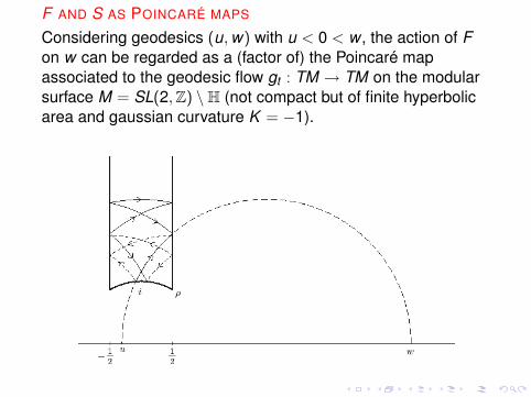
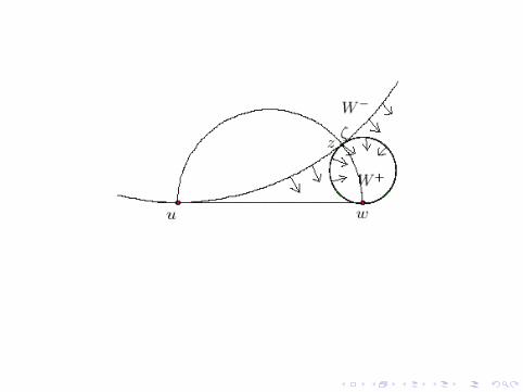
Considering geodesics (u, w) with u < 0 < w , the action of Fon w can be regarded as a (factor of) the Poincaré mapassociated to the geodesic flow gt : TM → TM on the modularsurface M = SL(2, Z) \H (not compact but of finite hyperbolicarea and gaussian curvature K = −1).
F AND S AS POINCARÉ MAPS
Considering geodesics (u, w) with u < 0 < w , the action of Fon w can be regarded as a (factor of) the Poincaré mapassociated to the geodesic flow gt : TM → TM on the modularsurface M = SL(2, Z) \H (not compact but of finite hyperbolicarea and gaussian curvature K = −1).
F AND S AS POINCARÉ MAPS
Considering geodesics (u, w) with u < 0 < w , the action of Fon w can be regarded as a (factor of) the Poincaré mapassociated to the geodesic flow gt : TM → TM on the modularsurface M = SL(2, Z) \H (not compact but of finite hyperbolicarea and gaussian curvature K = −1).
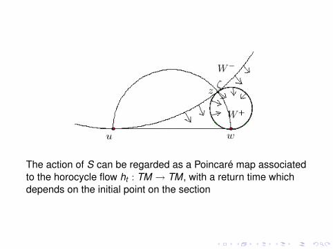
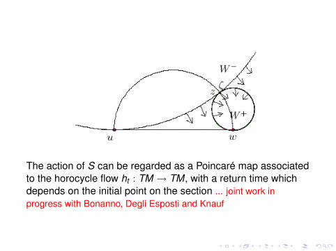
The action of S can be regarded as a Poincaré map associatedto the horocycle flow ht : TM → TM, with a return time whichdepends on the initial point on the section ... joint work inprogress with Bonanno, Degli Esposti and Knauf
The action of S can be regarded as a Poincaré map associatedto the horocycle flow ht : TM → TM, with a return time whichdepends on the initial point on the section
... joint work inprogress with Bonanno, Degli Esposti and Knauf
The action of S can be regarded as a Poincaré map associatedto the horocycle flow ht : TM → TM, with a return time whichdepends on the initial point on the section ... joint work inprogress with Bonanno, Degli Esposti and Knauf
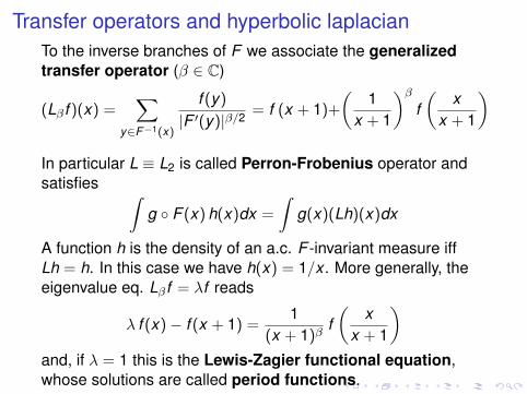
Transfer operators and hyperbolic laplacian
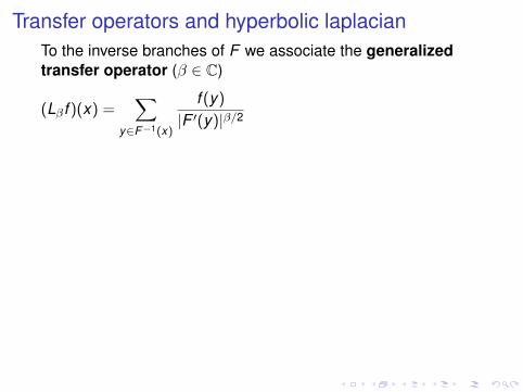
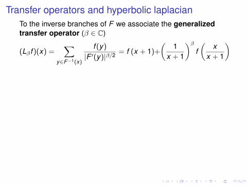
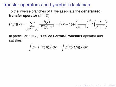
To the inverse branches of F we associate the generalizedtransfer operator (β ∈ C)
(Lβf )(x) =∑
y∈F−1(x)
f (y)
|F ′(y)|β/2 = f (x + 1)+
(1
x + 1
)β
f(
xx + 1
)
In particular L ≡ L2 is called Perron-Frobenius operator andsatisfies ∫
g ◦ F (x) h(x)dx =
∫g(x)(Lh)(x)dx
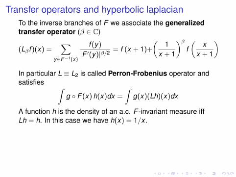
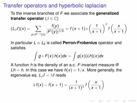
A function h is the density of an a.c. F -invariant measure iffLh = h. In this case we have h(x) = 1/x . More generally, theeigenvalue eq. Lβf = λf reads
λ f (x)− f (x + 1) =1
(x + 1)βf(
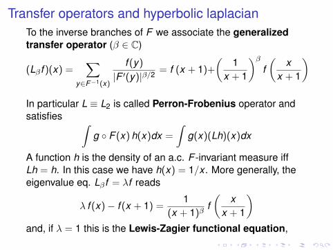
xx + 1
)and, if λ = 1 this is the Lewis-Zagier functional equation,whose solutions are called period functions.
Transfer operators and hyperbolic laplacianTo the inverse branches of F we associate the generalizedtransfer operator (β ∈ C)
(Lβf )(x) =∑
y∈F−1(x)
f (y)
|F ′(y)|β/2 = f (x + 1)+
(1
x + 1
)β
f(
xx + 1
)
In particular L ≡ L2 is called Perron-Frobenius operator andsatisfies ∫
g ◦ F (x) h(x)dx =
∫g(x)(Lh)(x)dx
A function h is the density of an a.c. F -invariant measure iffLh = h. In this case we have h(x) = 1/x . More generally, theeigenvalue eq. Lβf = λf reads
λ f (x)− f (x + 1) =1
(x + 1)βf(
xx + 1
)and, if λ = 1 this is the Lewis-Zagier functional equation,whose solutions are called period functions.
Transfer operators and hyperbolic laplacianTo the inverse branches of F we associate the generalizedtransfer operator (β ∈ C)
(Lβ f )(x) =∑
y∈F−1(x)
f (y)
|F ′(y)|β/2
= f (x + 1)+
(1
x + 1
)β
f(
xx + 1
)
In particular L ≡ L2 is called Perron-Frobenius operator andsatisfies ∫
g ◦ F (x) h(x)dx =
∫g(x)(Lh)(x)dx
A function h is the density of an a.c. F -invariant measure iffLh = h. In this case we have h(x) = 1/x . More generally, theeigenvalue eq. Lβf = λf reads
λ f (x)− f (x + 1) =1
(x + 1)βf(
xx + 1
)and, if λ = 1 this is the Lewis-Zagier functional equation,whose solutions are called period functions.
Transfer operators and hyperbolic laplacianTo the inverse branches of F we associate the generalizedtransfer operator (β ∈ C)
(Lβ f )(x) =∑
y∈F−1(x)
f (y)
|F ′(y)|β/2 = f (x + 1)+
(1
x + 1
)β
f(
xx + 1
)
In particular L ≡ L2 is called Perron-Frobenius operator andsatisfies ∫
g ◦ F (x) h(x)dx =
∫g(x)(Lh)(x)dx
A function h is the density of an a.c. F -invariant measure iffLh = h. In this case we have h(x) = 1/x . More generally, theeigenvalue eq. Lβf = λf reads
λ f (x)− f (x + 1) =1
(x + 1)βf(
xx + 1
)and, if λ = 1 this is the Lewis-Zagier functional equation,whose solutions are called period functions.
Transfer operators and hyperbolic laplacianTo the inverse branches of F we associate the generalizedtransfer operator (β ∈ C)
(Lβ f )(x) =∑
y∈F−1(x)
f (y)
|F ′(y)|β/2 = f (x + 1)+
(1
x + 1
)β
f(
xx + 1
)
In particular L ≡ L2 is called Perron-Frobenius operator andsatisfies ∫
g ◦ F (x) h(x)dx =
∫g(x)(Lh)(x)dx
A function h is the density of an a.c. F -invariant measure iffLh = h. In this case we have h(x) = 1/x .
More generally, theeigenvalue eq. Lβf = λf reads
λ f (x)− f (x + 1) =1
(x + 1)βf(
xx + 1
)and, if λ = 1 this is the Lewis-Zagier functional equation,whose solutions are called period functions.
Transfer operators and hyperbolic laplacianTo the inverse branches of F we associate the generalizedtransfer operator (β ∈ C)
(Lβ f )(x) =∑
y∈F−1(x)
f (y)
|F ′(y)|β/2 = f (x + 1)+
(1
x + 1
)β
f(
xx + 1
)
In particular L ≡ L2 is called Perron-Frobenius operator andsatisfies ∫
g ◦ F (x) h(x)dx =
∫g(x)(Lh)(x)dx
A function h is the density of an a.c. F -invariant measure iffLh = h. In this case we have h(x) = 1/x . More generally, theeigenvalue eq. Lβ f = λf reads
λ f (x)− f (x + 1) =1
(x + 1)βf(
xx + 1
)
and, if λ = 1 this is the Lewis-Zagier functional equation,whose solutions are called period functions.
Transfer operators and hyperbolic laplacianTo the inverse branches of F we associate the generalizedtransfer operator (β ∈ C)
(Lβ f )(x) =∑
y∈F−1(x)
f (y)
|F ′(y)|β/2 = f (x + 1)+
(1
x + 1
)β
f(
xx + 1
)
In particular L ≡ L2 is called Perron-Frobenius operator andsatisfies ∫
g ◦ F (x) h(x)dx =
∫g(x)(Lh)(x)dx
A function h is the density of an a.c. F -invariant measure iffLh = h. In this case we have h(x) = 1/x . More generally, theeigenvalue eq. Lβ f = λf reads
λ f (x)− f (x + 1) =1
(x + 1)βf(
xx + 1
)and, if λ = 1 this is the Lewis-Zagier functional equation,
whose solutions are called period functions.
Transfer operators and hyperbolic laplacianTo the inverse branches of F we associate the generalizedtransfer operator (β ∈ C)
(Lβ f )(x) =∑
y∈F−1(x)
f (y)
|F ′(y)|β/2 = f (x + 1)+
(1
x + 1
)β
f(
xx + 1
)
In particular L ≡ L2 is called Perron-Frobenius operator andsatisfies ∫
g ◦ F (x) h(x)dx =
∫g(x)(Lh)(x)dx
A function h is the density of an a.c. F -invariant measure iffLh = h. In this case we have h(x) = 1/x . More generally, theeigenvalue eq. Lβ f = λf reads
λ f (x)− f (x + 1) =1
(x + 1)βf(
xx + 1
)and, if λ = 1 this is the Lewis-Zagier functional equation,whose solutions are called period functions.
A Maass wave form of parameter s ∈ C is a SL(2, Z)-invariantfct u : H → C, vanishing for y →∞ and satisfying∆u = s(1− s)u where ∆ = y2(∂2
x + ∂2y ) is the hyperbolic
Laplacian on H.
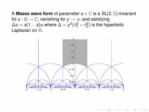
A Maass wave form of parameter s ∈ C is a SL(2, Z)-invariantfct u : H → C, vanishing for y →∞ and satisfying∆u = s(1− s)u where ∆ = y2(∂2
x + ∂2y ) is the hyperbolic
Laplacian on H.
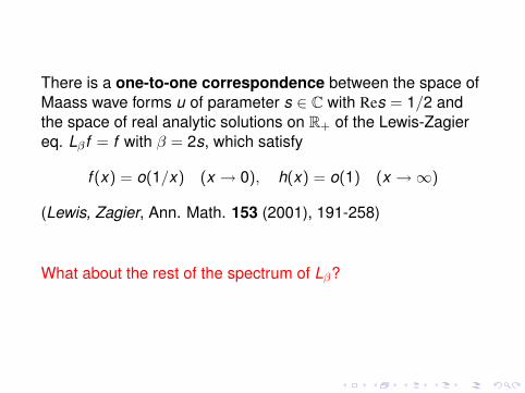
There is a one-to-one correspondence between the space ofMaass wave forms u of parameter s ∈ C with Res = 1/2 andthe space of real analytic solutions on R+ of the Lewis-Zagiereq. Lβf = f with β = 2s, which satisfy
f (x) = o(1/x) (x → 0), h(x) = o(1) (x →∞)
(Lewis, Zagier, Ann. Math. 153 (2001), 191-258)
What about the rest of the spectrum of Lβ?
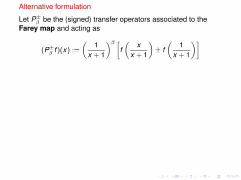
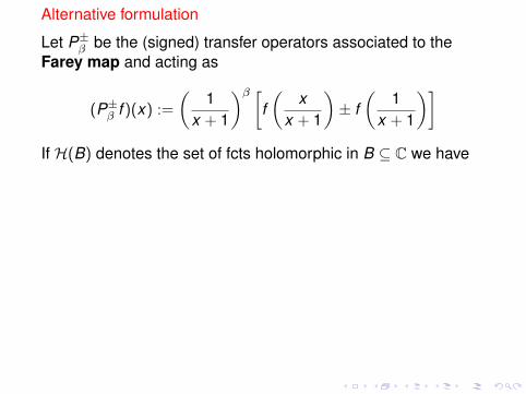
Alternative formulation
Let P±β be the (signed) transfer operators associated to the
Farey map and acting as
(P±β f )(x) :=
(1
x + 1
)β [f(
xx + 1
)± f(
1x + 1
)]If H(B) denotes the set of fcts holomorphic in B ⊆ C we have
I If f ∈ H({|z − 1| < 1}) then P±β f ∈ H({Rez > 0})
I If P±β f = λf with λ 6= 0 then Jβf = ±f , with
(Jβf )(z) :=1zβ
f(
1z
)Therefore the eigenvalue eqs. P±
β f = λ f are bothequivalent to Lβf = λf
I If u is a Maass form s.t. u(x + iy) = ±u(−x + iy) thenP±
β f = f with β = 2s
Alternative formulation
Let P±β be the (signed) transfer operators associated to the
Farey map and acting as
(P±β f )(x) :=
(1
x + 1
)β [f(
xx + 1
)± f(
1x + 1
)]
If H(B) denotes the set of fcts holomorphic in B ⊆ C we have
I If f ∈ H({|z − 1| < 1}) then P±β f ∈ H({Rez > 0})
I If P±β f = λf with λ 6= 0 then Jβf = ±f , with
(Jβf )(z) :=1zβ
f(
1z
)Therefore the eigenvalue eqs. P±
β f = λ f are bothequivalent to Lβf = λf
I If u is a Maass form s.t. u(x + iy) = ±u(−x + iy) thenP±
β f = f with β = 2s
Alternative formulation
Let P±β be the (signed) transfer operators associated to the
Farey map and acting as
(P±β f )(x) :=
(1
x + 1
)β [f(
xx + 1
)± f(
1x + 1
)]If H(B) denotes the set of fcts holomorphic in B ⊆ C we have
I If f ∈ H({|z − 1| < 1}) then P±β f ∈ H({Rez > 0})
I If P±β f = λf with λ 6= 0 then Jβf = ±f , with
(Jβf )(z) :=1zβ
f(
1z
)Therefore the eigenvalue eqs. P±
β f = λ f are bothequivalent to Lβf = λf
I If u is a Maass form s.t. u(x + iy) = ±u(−x + iy) thenP±
β f = f with β = 2s
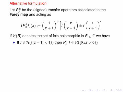
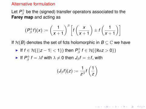
Alternative formulation
Let P±β be the (signed) transfer operators associated to the
Farey map and acting as
(P±β f )(x) :=
(1
x + 1
)β [f(
xx + 1
)± f(
1x + 1
)]If H(B) denotes the set of fcts holomorphic in B ⊆ C we have
I If f ∈ H({|z − 1| < 1}) then P±β f ∈ H({Rez > 0})
I If P±β f = λf with λ 6= 0 then Jβf = ±f , with
(Jβ f )(z) :=1zβ
f(
1z
)
Therefore the eigenvalue eqs. P±β f = λ f are both
equivalent to Lβf = λfI If u is a Maass form s.t. u(x + iy) = ±u(−x + iy) then
P±β f = f with β = 2s
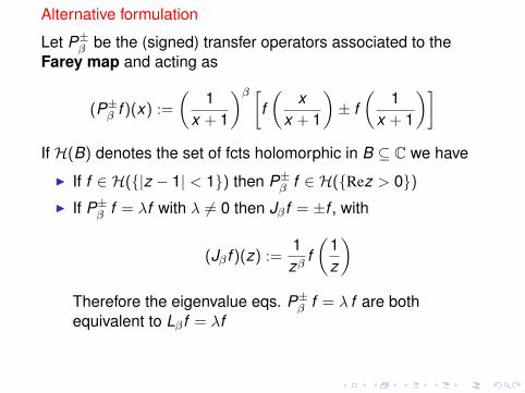
Alternative formulation
Let P±β be the (signed) transfer operators associated to the
Farey map and acting as
(P±β f )(x) :=
(1
x + 1
)β [f(
xx + 1
)± f(
1x + 1
)]If H(B) denotes the set of fcts holomorphic in B ⊆ C we have
I If f ∈ H({|z − 1| < 1}) then P±β f ∈ H({Rez > 0})
I If P±β f = λf with λ 6= 0 then Jβf = ±f , with
(Jβ f )(z) :=1zβ
f(
1z
)Therefore the eigenvalue eqs. P±
β f = λ f are bothequivalent to Lβf = λf
I If u is a Maass form s.t. u(x + iy) = ±u(−x + iy) thenP±
β f = f with β = 2s
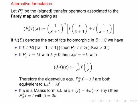
Alternative formulation
Let P±β be the (signed) transfer operators associated to the
Farey map and acting as
(P±β f )(x) :=
(1
x + 1
)β [f(
xx + 1
)± f(
1x + 1
)]If H(B) denotes the set of fcts holomorphic in B ⊆ C we have
I If f ∈ H({|z − 1| < 1}) then P±β f ∈ H({Rez > 0})
I If P±β f = λf with λ 6= 0 then Jβf = ±f , with
(Jβ f )(z) :=1zβ
f(
1z
)Therefore the eigenvalue eqs. P±
β f = λ f are bothequivalent to Lβf = λf
I If u is a Maass form s.t. u(x + iy) = ±u(−x + iy) thenP±
β f = f with β = 2s
SOME SPECTRAL PROPERTIES OF P±β
Let Hβ be the Hilbert space of functions f ∈ H({|z − 1| < 1})and such that
f (x) = B [ϕ](x) :=1
xβ
∫ ∞
0e−
tx etϕ(t)mβ(dt)
with ϕ ∈ L2(mβ) and mβ(dt) = tβ−1e−tdt .
THEOREM (I., 2003) P±β B [ϕ] = B [(M + N)ϕ] with
M ϕ(t) = e−tϕ(t) , Nϕ(t) =
∫ ∞
0
Jβ−1
(2√
st)
(st)(β−1)/2 ϕ(s) mβ(ds)
THEOREM (Bonanno, Graffi, I., 2007) For each β ∈ (0,∞) theoperators P±
β : Hβ → Hβ are bounded, self-adjoint andisospectral. Their spectrum is {0} ∪ (0, 1], with (0, 1] purely a.c.
SOME SPECTRAL PROPERTIES OF P±β
Let Hβ be the Hilbert space of functions f ∈ H({|z − 1| < 1})
and such that
f (x) = B [ϕ](x) :=1
xβ
∫ ∞
0e−
tx etϕ(t)mβ(dt)
with ϕ ∈ L2(mβ) and mβ(dt) = tβ−1e−tdt .
THEOREM (I., 2003) P±β B [ϕ] = B [(M + N)ϕ] with
M ϕ(t) = e−tϕ(t) , Nϕ(t) =
∫ ∞
0
Jβ−1
(2√
st)
(st)(β−1)/2 ϕ(s) mβ(ds)
THEOREM (Bonanno, Graffi, I., 2007) For each β ∈ (0,∞) theoperators P±
β : Hβ → Hβ are bounded, self-adjoint andisospectral. Their spectrum is {0} ∪ (0, 1], with (0, 1] purely a.c.
SOME SPECTRAL PROPERTIES OF P±β
Let Hβ be the Hilbert space of functions f ∈ H({|z − 1| < 1})and such that
f (x) = B [ϕ](x) :=1
xβ
∫ ∞
0e−
tx etϕ(t)mβ(dt)
with ϕ ∈ L2(mβ) and mβ(dt) = tβ−1e−tdt .
THEOREM (I., 2003) P±β B [ϕ] = B [(M + N)ϕ] with
M ϕ(t) = e−tϕ(t) , Nϕ(t) =
∫ ∞
0
Jβ−1
(2√
st)
(st)(β−1)/2 ϕ(s) mβ(ds)
THEOREM (Bonanno, Graffi, I., 2007) For each β ∈ (0,∞) theoperators P±
β : Hβ → Hβ are bounded, self-adjoint andisospectral. Their spectrum is {0} ∪ (0, 1], with (0, 1] purely a.c.
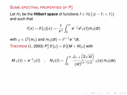
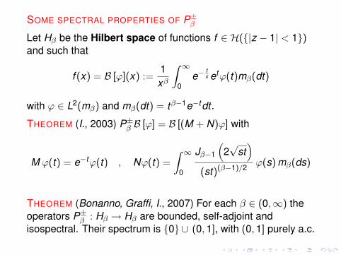

Some perspectives
I Generalized eigenfcts of P±β with β ∈ (0,∞)
I Spectrum of P±β with β ∈ C
I Tree expansion and analytic continuation of (generalized)Ruelle and Selberg zeta functions
I Harmonic functions and martingalesI Integrability of spin models
Some perspectives
I Generalized eigenfcts of P±β with β ∈ (0,∞)
I Spectrum of P±β with β ∈ C
I Tree expansion and analytic continuation of (generalized)Ruelle and Selberg zeta functions
I Harmonic functions and martingalesI Integrability of spin models
Some perspectives
I Generalized eigenfcts of P±β with β ∈ (0,∞)
I Spectrum of P±β with β ∈ C
I Tree expansion and analytic continuation of (generalized)Ruelle and Selberg zeta functions
I Harmonic functions and martingalesI Integrability of spin models
Some perspectives
I Generalized eigenfcts of P±β with β ∈ (0,∞)
I Spectrum of P±β with β ∈ C
I Tree expansion and analytic continuation of (generalized)Ruelle and Selberg zeta functions
I Harmonic functions and martingalesI Integrability of spin models
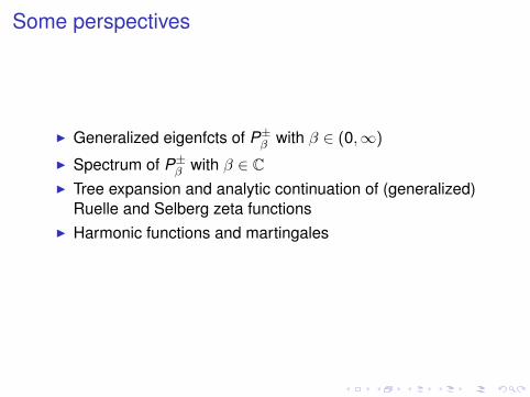
Some perspectives
I Generalized eigenfcts of P±β with β ∈ (0,∞)
I Spectrum of P±β with β ∈ C
I Tree expansion and analytic continuation of (generalized)Ruelle and Selberg zeta functions
I Harmonic functions and martingales
I Integrability of spin models
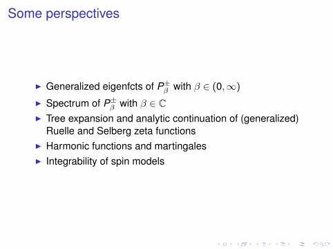
Some perspectives
I Generalized eigenfcts of P±β with β ∈ (0,∞)
I Spectrum of P±β with β ∈ C
I Tree expansion and analytic continuation of (generalized)Ruelle and Selberg zeta functions
I Harmonic functions and martingalesI Integrability of spin models

Some perspectives
I Generalized eigenfcts of P±β with β ∈ (0,∞)
I Spectrum of P±β with β ∈ C
I Tree expansion and analytic continuation of (generalized)Ruelle and Selberg zeta functions
I Harmonic functions and martingalesI Integrability of spin models


![Rationals, Periodicity Chaos: Pythagorean View Co ]ecture ...downloads.hindawi.com/journals/ddns/2000/652540.pdf · Rationals, Periodicity and Chaos: APythagoreanView and a Co ]ecture](https://img.pdfslide.us/doc/110x75/5ed92b586714ca7f47694677/rationals-periodicity-chaos-pythagorean-view-co-ecture-rationals-periodicity.jpg)