Embed Size (px)
Citation preview
Preface
The objective with this thesis is to assess recent advances in decision theory under uncertainty and
to find out whether these can be used as an extension to the decision analysis normally performed
in the industry.
Oil companies put a lot of effort into reducing the uncertainties in their decision making and invest
in extensive exploration and front end study activities prior to project sanction. After a project is
sanctioned the companies select reliable contractors and monitor performance closely to reduce
uncertainties and ensure predictable project execution. Decision analysis may be performed to
support decision making at several of these key stages of a project development where identified
uncertainties are described by the use of probability distributions and Monte Carlo simulations.
The analysis results are then normally represented by an uncertainty range and an expected value
of the observable quantities. A qualitative judgement process or management review process is
then performed to define a margin that addresses the uncertainty in the results.
Recent advances in decision theory do however have a potential to extend the quantitative
modelling approach beyond current decision analysis practise. In this thesis, recent advances in
decision theory models have been assessed and an attempt is made to capture the uncertainties and
define a single equivalent sure amount for various types of decision problems. The single
equivalent sure amount value defined by these extended decision analysis models can potentially
support rational decision making and serve as a potential improvement to the management review
process of decisions associated with uncertainty.
There are numerous papers to be found that describe normative and descriptive theoretical models
for decision analysis, but very few of these are able to translate their theory into practical
applications. The paper from Borgonovo & Marinacci (2015) that describe decisions under
ambiguity do however stand out as an exception to the rest. This excellent paper describes the
theoretical basis and illustrates this theory with numerical analysis of relevant decision problems.
In-depth interviews of a selected group of decision makers are included in the qualitative research
to assess whether the theoretical models of decision analysis associated with uncertainty are known
and used by the industry. Scenarios were also included in the in-depth interviews in order to see
how consistent decision makers are when subject to decision problems associated with various
forms of uncertainty.
Decision problems have been analysed that includes uncertainties relating to business risk, cost
risk, production risk and accident risk. The theory and methods for decision analysis under risk
and ambiguity are intended to give useful information that support rational decision making and
improve the basis for decision support.
Per Inge Nag
11.06.2018
An Assessment of Ambiguity in Decision Analysis June 2018
Student No 238030 Page 1 of 106
Table of contents 1. Introduction ........................................................................................................................... 4
1.1 Background ..................................................................................................................... 5
1.2 Scope and limitations ..................................................................................................... 6
2. Theoretical models for decision analysis with ambiguity .................................................. 8
2.1 Literature review ............................................................................................................ 8
2.2 A closer look at relevant theoretical models .............................................................. 12
3 Qualitative research of decision making practice ............................................................. 27
3.1 Methodology ................................................................................................................. 27
3.2 Results ........................................................................................................................... 29
4 A business risk decision problem- Race or withdraw ...................................................... 39
4.1 Introduction .................................................................................................................. 39
4.2 Expected Value ............................................................................................................. 39
4.3 Smooth ambiguity aversion ......................................................................................... 40
4.4 Risk aversion ................................................................................................................. 40
4.5 Extreme Risk and Ambiguity aversion ...................................................................... 41
4.6 Decision maker’s preferences for the Carter Racing ................................................ 41
5 A Cost Risk Decision Problem - Project contingency ...................................................... 42
5.1 Introduction .................................................................................................................. 42
5.2 Probability distributions of input variables ............................................................... 42
5.3 Expected value and confidence interval ..................................................................... 43
5.4 Smooth ambiguity aversion model.............................................................................. 43
5.5 Risk aversion model ..................................................................................................... 45
5.6 Resulting confidence levels for the project cost estimate .......................................... 45
6 A Production Risk Decision Problem - Ranking of scenarios ......................................... 48
6.1 Introduction .................................................................................................................. 48
6.2 Probability distributions of input variables ............................................................... 48
6.3 Production profiles ....................................................................................................... 49
6.4 Expected value and confidence interval for the net present values ......................... 49
6.5 Smooth ambiguity aversion model.............................................................................. 49
6.6 Risk aversion model ..................................................................................................... 51
6.7 Extreme risk and ambiguity aversion model ............................................................. 51
An Assessment of Ambiguity in Decision Analysis June 2018
Student No 238030 Page 2 of 106
6.8 Decision maker’s preferences for the production scenarios..................................... 51
7 An Accident Risk Decision Problem – The need for safety valve ................................... 58
7.1 Introduction .................................................................................................................. 58
7.2 Probability distributions of input variables ............................................................... 58
7.3 Production profiles ....................................................................................................... 59
7.4 Expected value and confidence interval given no riser failure ................................ 59
7.5 Consequence of riser failure ........................................................................................ 60
7.6 Certainty Equivalent using the Expected Monetary Value ...................................... 60
7.7 Certainty Equivalent using the Smooth Ambiguity Aversion Model ...................... 61
7.7.1 Certainty equivalent conditional of no riser failure .............................................. 61
7.7.2 Certainty equivalent unconditional of riser failure ............................................... 62
7.8 Certainty Equivalent using the Risk Aversion model ............................................... 63
7.9 Certainty Equivalent using the Extreme Risk and Ambiguity Aversion model .... 64
7.10 Decision maker’s preferences for SSIV .................................................................. 64
8 Analysis and discussions ..................................................................................................... 66
8.1 Decision theory versus decision making practice ...................................................... 66
8.2 Decision analysis of business risk ................................................................................ 67
8.3 Decision analysis of cost risk ....................................................................................... 67
8.4 Decision analysis of production risk ........................................................................... 67
8.5 Decision analysis of accidental risk............................................................................. 68
8.6 Use of risk aversion models ......................................................................................... 68
8.7 Risk and ambiguity aversion parameters .................................................................. 69
8.8 Beyond the economic perspective ............................................................................... 69
8.9 A project manager’s recommendation ....................................................................... 70
9 Conclusion ............................................................................................................................ 71
10 References ............................................................................................................................. 72
Appendix A – Detailed analysis of the Ellsberg three-color problem .................................... 77
A.1 Exact quadratic solution of the variance of the expected payoff ............................. 77
A.2 Approximate quadratic solution of the variance of the expected payoff ................ 84
A.3 Solving the smooth ambiguity functional ................................................................... 86
Appendix B – Detailed analysis of the Carter Racing Model ................................................. 91
B.1 Second order probability distribution ........................................................................ 91
An Assessment of Ambiguity in Decision Analysis June 2018
Student No 238030 Page 3 of 106
B.2 Expected value .............................................................................................................. 91
B.3 Risk aversion ................................................................................................................. 92
B.4 Wald Maximin Functional........................................................................................... 92
B.5 Risk and ambiguity aversion expressed by the KMM utility ................................... 92
B.6 Certainty equivalent as the inverse of the KMM utility ........................................... 94
B.7 Balancing the share of risk premium and ambiguity premium ............................... 94
B.8 Realisations and integration in Excel ........................................................................ 98
Appendix C – Interview Question Protocol ............................................................................ 105
An Assessment of Ambiguity in Decision Analysis June 2018
Student No 238030 Page 4 of 106
1. Introduction
We all have to make a lot of important decisions during our lifetime. These decisions are typically
associated with uncertainties and can among other things be related to choice of friends, lifetime
partner, education, career or where to settle down and when to retire. Some of these uncertainties
are known phenomena that can be reasonably well defined by random variations. Other types of
uncertainties are unknown and are not that easy to define by random variations based on the
information available at the time of the decision. These unknown or un-measureable uncertainties
can for example be related to the choice to move to a new city where you do not know anyone or
the choice of an education where you do not have any prior knowledge. In business life, oil
companies are also faced with these types of measureable and un-measureable uncertainties in
their decision making. The measureable uncertainties are normally defined by the use of
probability distributions that describe the random variation of the relevant phenomena. The un-
measureable uncertainties are more difficult to describe by the use of probability distribution as
these refers to unknown phenomena’s as a result of lack of information. Consequently if more
relevant information is made available, the un-measureable uncertainty can be reduced. Oil
companies do therefore invest in several activities in order to reduce the un-measureable
uncertainties in their decision making. Exploration and appraisal wells and seismic surveys are
performed to collect as much information as possible about the location and size of a reservoir.
Front end studies are performed to define the solution and cost of a field development project prior
to project sanction. Information of potential contractor’s previous experience and performance is
gathered and evaluated by the oil companies prior to contract awards to ensure predictable project
execution within time and cost.
Sometimes in our lives, we take wrong decisions due to ignorance or simply bad judgement. We
then have to live with the consequences which could eventually be broken relationships, lost
opportunities or other types of losses. In the business world, we also sometimes see that oil
companies make decisions that result in project delivery failures or lost production. These
decisions could also be a result of ignorance of the uncertainties or bad judgement of the potential
outcomes. This could for example be in relation to the choice of novel platform concepts or the
choice of contractors with limited or no experience with implementation of the function-based
regulations specific for the Norwegian Continental Shelf (NCS) as defined by the NORSOK1)
standards. We have in the past even seen projects consisting of novel platform concepts that are to
be delivered by contractors with limited or no NORSOK experience. In Stavanger Aftenblad, 8th
of May 2018, we can read about the decisions made in the 80’s and 90’s to place platform contracts
to yards in Asia. These Asian yards had limited NORSOK experience and it was probably not
known at the time how big impact this lack of NORSOK experience actually had on the project
delivery. In retrospect we can see that there are large cultural differences between how work is
managed and executed in a Norwegian and an Asian Yard.
1) The acronym NORSOK stands for “the Norwegian shelf’s competitive position”. The
NORSOK standards serve as references to the authorities regulations and have been in use since
1994 to ensure adequate safety, value adding and cost effectiveness within development and
operation of petroleum assets and activities.
An Assessment of Ambiguity in Decision Analysis June 2018
Student No 238030 Page 5 of 106
The cultural differences will also influence how the functional requirements given in Norwegian
rules and regulations are interpreted and implemented. Did the oil company consider that the prices
and schedules from an Asian yard had the same predictability as for a Norwegian Yard? The oil
companies were in these decision problems most likely faced with elements of un-measureable
uncertainties in relation to the consequence of poor knowledge and understanding of Norwegian
rules and regulations as defined by the NORSOK standards. These un-measureable uncertainties
were probability not properly captured by the decision analysis available at the time. The
consequences of some of these decisions were large cost overruns, significant delays and poor
quality. A significant amount of rework that caused further delays also had to be done by
Norwegian yards to ensure that the new platforms satisfied the mandatory functional requirements.
There are also recent examples of platform projects where the implementation of mandatory
functional requirements are suspended to the offshore location. These decisions to move large
portions of the mechanical completion to the offshore location opens up for new both measurable
and un-measureable uncertainties with an increased potential for cost overruns and delays.
One of the reasons that Norwegian Yards gets a higher share of platform contracts in the recent
years could be that the un-measureable uncertainties with respect to the use of Asian yard are
shifted to measureable uncertainties in recent decision analysis. Recent decision analysis can then
describe random variations for this phenomena of measureable uncertainty based on the past
experience of de facto negative outcomes.
With respect to choice of facility concepts we can also see that oil companies may have different
preferences. A recent article in Dagens Næringsliv, 7th of May 2018, refers to a current discussion
between two oil companies on the concept selection for a new field development. One of the
license partners wants to have a single integrated process platform while the other license partner
wants to have several smaller wellhead platforms. These different views could be caused by
different economic drivers. The different views could also be caused by subjective preferences and
experiences or biased views to the un-measureable uncertainties related to the execution and
production of the proposed facility concepts. The decision analysis results will then largely depend
on the respective oil company’s assessments of the level of un-measureable uncertainties and how
these are balanced with their subjective preferences and experiences.
The un-measureable uncertainties described in the above examples are, in a decision analysis
context, commonly termed as ambiguity. Ambiguity can both refer to non-uniqueness, inability or
lack of information to describe the uncertainty of a decision problem. The measureable
uncertainties are, on the other hand, commonly termed as risk in a decision analysis context.
The objective with this thesis is to assess if quantitative models can be introduced to give
preferences and margins when subject to both measureable uncertainties (risk) and un-measureable
uncertainties (ambiguity). This assessment of quantitative models will be based on recent advances
in decision theories and can potentially provide useful additional decision support information
beyond current industry practice.
1.1 Background
A project manager may have to handle different types of decision problems and uncertainties in a
project’s life cycle. Common capital value processes are however implemented by the industry to
An Assessment of Ambiguity in Decision Analysis June 2018
Student No 238030 Page 6 of 106
capture uncertainty and ensure a staged maturing and definition of a project development. The
common capital value processes include the decision gates DG1, DG2 and DG3. Decision gate
DG1 is based on the uncertainties and the technical and cost accuracy described by the feasibility
study for a project development. Decision gate DG2 is based on the uncertainties and the technical
and cost accuracy described by the concept study for a project development. Decision gate DG3 is
based on the uncertainties and the technical and cost accuracy described by the FEED study for a
project development.
The types of decision problems that need to be assessed at the decision gates may involve economic
risks and accidental risks (Aven, 2012). The decision process that the project manager is expected
to follow is a value process for decision making under uncertainty (Aven, 2015). This decision
process starts with a definition of the decision problem and a description of the decision
alternatives. The next step in the decision process is to perform analysis and evaluations which
may include risk analyses and decision analyses.
In decision analysis, the element of risk and uncertainty are assessed by the use of probability
distributions and Monte Carlo simulations. The analysis results are normally represented by
expected values and confidence intervals that describe an uncertainty range of the observable
quantities. Normally the decision analysis stops with the description of the expected value and the
uncertainty range and a qualitative judgement is performed to define a margin to address the
uncertainty in the results. The risk and decision analyses and evaluations are subject to value based
assessments in the form of a management review and judgement process and a stakeholders review
process. The value based assessments are also evaluating and expected to take due account of
uncertainties that are not covered by the risk and decision analyses. These uncertainties can lead
to the implementation of additional precautionary or cautionary measures or other actions that will
be part of the final risk picture which will form the basis for the decision making.
In this thesis, the objective is to go one step further in the quantitative decision analysis and include
analytical models that define margins or premiums for risk and ambiguity. These margins or
premiums can be used to define a single equivalent sure amount as additional information to the
expected value and uncertainty range. This information about an equivalent sure amount can
potentially be used as a guide for rational decision making when qualitative judgements are
performed.
1.2 Scope and limitations
This thesis includes a detailed review of relevant decision theory, qualitative research in the form
of peer group interviews and quantitative assessments of selected decision problems. The
assessments performed are referring to the analytical and bureaucratic decision setting (Aven,
2012) where decisions are made based on strategic decision analysis which may include detailed
processes of identifying alternatives and based on analysis of probabilities and consequences.
The concepts and theories relating to decision analysis with risk and ambiguity have been reviewed
and included in section 2. References have been made to relevant sources of information consisting
of articles and books found through the UiS library databases. The detailed review is performed
with an emphasis on identifying quantiative models and methods that can be used by a project
An Assessment of Ambiguity in Decision Analysis June 2018
Student No 238030 Page 7 of 106
manager to perform a rational subjective assessment along with an estimate of the uncertainty for
his decision alternatives. The relevant decision theories are selected based on the ability to identify
preferences in outcome sets where the occurrence of only some of the outcomes have a defined
probability. The other outcomes are then subject to ambiguity in the form of undefined probability.
The descriptive theories of decision making is only briefly described as these need to be supported
by extensive specific qualitative research that is beyond the scope of this thesis.
The research question that has been driving the qualitative research is basically to assess if decision
theory under ambiguity is known and used by the industry. The quality research performed has
been in the form of in-depth interviews of a selected peer group. The results of the qualitative
research described in section 3 are based on a subjective assessment of the responses from the
members of the peer group.
Quantiative assessments of selected decision problems in relation to economic risk and accident
risk have been performed. In section 4, a business risk decision problem related to running or
withdrawing from a car race has been analysed. In section 5, analysis is performed for a typical
cost risk decision problem of defining the project contingency for a project cost estimate. In section
6, a production risk decision problem is analysed regarding the ranking of project development
scenarios. In section 7, a decision problem associated with accident risk is included that analyse
whether or not a subsea safety isolation valve (SSIV) need to be installed.
Analysis and discussions to the above assessments of decision theory and their application are
included in section 8. A conclusion of the assessment of ambiguity in decision analysis is given in
section 9.
An Assessment of Ambiguity in Decision Analysis June 2018
Student No 238030 Page 8 of 106
2. Theoretical models for decision analysis with ambiguity
A literature review is performed to identify potential decision theories that address uncertainties
in a decision problem. A detailed review and screening of the identified potential decision theories
is done to see whether these can define preferences in a three-color decision problem (Ellsberg,
1961) with elements of both risk and ambiguity.
2.1 Literature review
The literature review identify the relevant theoretical basis for decision analysis under uncertainty
and how these theories correspond and interface with general theories of risk and uncertainty. The
literature review also identify the relevant basis and standards for decision problems in relation to
business risk, production risk, cost risk and accidental risk.
2.1.1 Decision theories
The expected value method is commonly used in decision analysis and originates from portfolio
theory (Markowitz, 1952), (Abrahamsen, et al., 2004), (Aven, 2012) . The expected value is
represented by the average value of the portfolio. The variance of the portfolio is represented by
the sum of the average variance of the non-systematic risk and the covariance of the systematic
risk. The expected value method is recommended used in decision problems associated with low
uncertainty (Soerskaar & Abrahamsen, 2017). The expected value method has remained as a pillar
in value propositions and net-present value analysis (Bratvold & Begg, 2009), (Willigers, et al.,
2017).
The expected utility theory (von Neumann & Morgenstern, 1947) and the subjective expected
utility theory (Savage, 1954) also referred to as Bayesian decision theory (Lindley, 1985) have for
a long period been the governing framework of decision theory when associated with rational
decision making under uncertainty. The subjective expected utility was defined as a function of
the subjective probabilities (Ramsey, 1931) and the utility functions (von Neumann &
Morgenstern, 1947) for an outcome set. A reduced state space for the subjective expected utility
was introduced by a two-staged lottery and horse-race definition of the subjective probabilities
(Anscombe & Aumann, 1963).
The Wald maximin criterion (Wald, 1949) define the preferences for an extreme risk and
ambiguity averse decision maker. The maximin criterion has been further generalised in maxmin
expected utility which define a function of multiple priors and outcomes (Gilboa & Schmeidler,
1989).
The axioms and postulates that represent the basis for the subjective expected theory of rational
decision making have been challenged over the years. Case studies were presented in 1953 by
Allais and in 1961 by Ellsberg (1961) that showed that a decision maker may struggle to select his
preferences when faced with un-measureable uncertainty in his decision problems.
Descriptive decision theories were developed to capture the cognitive thinking behind human
action based on decision weighting and non-additive probabilities (Quiggin, 1982), (Schmeidler,
1989), (Kahneman & Tversky, 1992), (Tuthill & Frechette, 2002), (Hampel, 2009), (Aerts &
Sozzo, 2015), (dos Santos, et al., 2018). It was found that people in both experimental and real life
situations do not conform to the axioms and postulates that the expected utility and the subjective
An Assessment of Ambiguity in Decision Analysis June 2018
Student No 238030 Page 9 of 106
expected utility are based on (Quiggin, 1982). Anticipated utility theory (Quiggin, 1982) and the
non-expected utility theories (Tuthill & Frechette, 2002); weighted expected utility, rank
dependent utility, also called Choquet expected utility, and cumulative prospect theory was
therefore introduced. These theories are associated with a weaker set of axioms than the expected
utility axioms. The weaker axioms permits the use of decision weights of non-additive
probabilities. Tests of the Choquet expected utility (Mangelsdorff & Weber, 1994) concluded that
the Choquet expected utility was not superior to the expected utility theory when defining
preferences in the Ellsberg three-color problem (Ellsberg, 1961).
The normative and descriptive decision theories seem to have very different perspectives. The
normative decision theories are based on a set of axioms and postulates that define rational decision
making (Howard, 1988). The descriptive decision theories are based on cognitive testing on how
people actual make their decisions (Howard, 1988). The descriptive decision theories are therefore
based on tests and case studies on how decision makers do behave as opposed to the normative
decision theory that prescribe how a decision maker should behave. The independence axiom and
the sure-thing principle defined in the normative decision theories are replaced by weaker axioms
in the descriptive decision theories to align with tested human behaviour (Howard, 1988). As
noted in Howard (1988), it is a descriptive fact that most of us can make mistakes in arithmetic
calculations, but it is the normative rules of arithmetic that allows us to recognize a mistake. A
similar relationship exists between normative and descriptive theories in decision analysis
(Howard, 1988). The acceptance of the normative decision theory thus allows us to recognize our
decision mistakes (Howard, 1988).
In recent decision theory literature (Klibanoff, et al., 2005), (Eichberger & Kelsey, 2007), (Gilboa
& Marinacci, 2011), (Etner, et al., 2012), (Klibanoff, et al., 2012), (Cerreia-Vioglio, et al., 2013a),
(Maccheroni, et al., 2013), (Borgonovo & Marinacci, 2015), (Hansen & Marinacci, 2016)
uncertainties are divided into two categories. Uncertainties that can be defined by a probability
distribution is termed “risk” while uncertainties where the decision maker is not able to specify a
unique probability distribution is termed “ambiguity”.
The Smooth Ambiguity Functional (Klibanoff, et al., 2005) and the Extended Arrow-Pratt
quadratic estimation method (Maccheroni, et al., 2013) are advances to the subjective expected
utility. These are developed to incorporate the elements of both “risk” and “ambiguity” and the
decision maker’s risk and ambiguity aversion in the analysis of a decision problem. The Smooth
Ambiguity Functional (Klibanoff, et al., 2005) introduces second order probabilities of the
predicted probability for an uncertain outcome. The second order probabilities are a probability
distribution that introduces a variation in the definition of the predicted probability. The Smooth
Ambiguity Functional calculates a risk and ambiguity premium for a decision problem (Klibanoff,
et al., 2005). The Extended Arrow-Pratt Quadratic estimation (Maccheroni, et al., 2013) can be
used to provide an estimate of the split between a premium of risk and a premium of ambiguity of
the risk and ambiguity premium found by the Smooth Ambiguity Functional.
Quantitative methods are introduced (Borgonovo & Marinacci, 2015) by the use of the Smooth
Ambiguity Functional (Klibanoff, et al., 2005) and the Extended Arrow-Pratt Quadratic estimation
An Assessment of Ambiguity in Decision Analysis June 2018
Student No 238030 Page 10 of 106
(Maccheroni, et al., 2013) to resolve the decision maker’s preferences in the Ellsberg three-color-
problem (Ellsberg, 1961) and the Carter racing decision problem (Brittain & Sitkin, 1990).
2.1.2 The bridge between risk and decision theory
In risk analysis literature (Ramsey, 1931), (Kaplan & Garrick, 1981), (Aven, 2012), (Aven, et al.,
2014), (Aven, 2014), (Aven, 2015), (Soerskaar & Abrahamsen, 2017) the term “risk” is
recommended to have a broader definition. Risk is here defined by the two main dimensions
consequences, (C), and uncertainties, (U) (Aven, 2015). The risk description is defined by
specified consequences and a descriptive measure of the uncertainty (Q). Probability distributions
are normally used as the descriptive measure of the uncertainty (Q), where subjective probabilities
are assigned to both of the categories of uncertainty described in the decision theory literature.
A clear distinction is however made between “aleatory” and “epistemic” uncertainty in risk
analysis (Aven, 2012), (Aven, et al., 2014). An aleatory uncertainty can be described by both
subjective and frequentist probabilities in order to describe a natural variation of a phenomena.
This type of phenomena can however, not necessarily be reduced as more information becomes
available. An epistemic uncertainty can only be described by subjective probabilities as this
uncertainty is a result of lack of information. The epistemic uncertainty can therefore be reduced
if more information becomes available.
The aleatory and epistemic uncertainties defined in risk analysis do represent an important bridge
between the risk analysis and the decision analysis that may result in improved decision support
(Pate-Cornell & Dillon, 2006), (Pate-Cornell, 2007), (Borgonovo, et al., 2015), (Borgonovo, et al.,
2016), (Borgonovo, et al., 2018).
2.1.3 Risk and ambiguity aversion
In the past, risk attitudes or risk tolerance have been subject to empirical studies and analysis within
the petroleum industry (Spetzler, 1968), (Walls, et al., 1995), (Walls & Dyer, 1996), within large
corporations (Howard, 1988), (Pate-Cornell & Fischbeck, 1992), (Smith, 2004) and within the
health sector (Treich, 2010). A decision-theoretic status on risk attitudes is presented by Baccelli
(2017).
Ambiguity and a decision maker’s attitude towards ambiguity were found by the experiments
introduced by Allais and Ellsberg (1961). Ambiguity refers to a decision situation under
uncertainty when there is incomplete information about the likelihood of events (Eichberger &
Kelsey, 2007). In the Ellsberg experiments it was found that the decision maker would have a
preference for betting on events with defined probability distributions (Ellsberg, 1961),
(Eichberger & Kelsey, 2007). The decision maker can be either ambiguity neutral or ambiguity
averse (Etner, et al., 2012). The dominating behavior for a decision maker in the gain domain
(upsides) is ambiguity aversion while the dominating behavior for a decision maker in the loss
domain (downside) is ambiguity neutrality (Etner, et al., 2012). Negative attitude or aversion
towards ambiguity do however not seem to hold in situations where the decision maker feels
comfortable with the situation despite the presence of unknown probabilities (Eichberger &
Kelsey, 2007).
An Assessment of Ambiguity in Decision Analysis June 2018
Student No 238030 Page 11 of 106
Risk and ambiguity aversion are included in the recent advances in decision theory (Klibanoff, et
al., 2005), (Maccheroni, et al., 2013), (Borgonovo & Marinacci, 2015).
2.1.4 Business risk decisions
The challenger launch decision (Brittain & Sitkin, 1990), (Liedtka, 1990) has been used by many
organisations as a case study for training in decision making exposed to risk and ambiguity. The
objective with this training in decision making is to address how actions derived from quantitative
analysis are implemented using organisational mechanisms and behavioural interventions (Brittain
& Sitkin, 1990).
Quantitative analysis performed for the Carter racing case (Borgonovo & Marinacci, 2015) is a
stylised example of a business risk decision that refers to the Challenger Launch Decision.
2.1.5 Production risk decisions
Production risk refers to uncertainties associated with a certain performance measure (Aven, 2012)
and can refer to potentially reduced production efficiency as a result of downtime caused by
equipment failures and maintenance or as a result of subsurface production issues. The production
system for a field development consists of complex subsystems for reservoir, wells and facilities.
These subsystems are typically treated independently in both design and operations (Chow &
Arnondin, 2000) and the relevant components of the system have historically been optimised on
the basis of the local subsystem instead of the overall global production system (Chow &
Arnondin, 2000). Risk based integrated production models are introduced (Chow & Arnondin,
2000), (Chow, et al., 2000) (Fassihi, et al., 2000) to quantify and manage uncertainty associated
with field-development design, implementation and operation.
2.1.6 Cost risk decisions
Cost risk refers to uncertainties associated with project cost estimates (Aven, 2012). Cost risk has
been analysed in cost engineering forums with the objective to improve the predictability of project
cost estimates (Dillon, et al., 2002), (Burger, 2003), (Sauser, et al., 2009), (Howell, et al., 2010),
(Olumide, et al., 2010), (Idrus, et al., 2011), (van Niekerk & Bekker, 2014). Standard practices on
the definitions and guidelines on the use of allowance, contingency and reserves in project cost
estimates for the building industry have been developed (ASTM-E1946, 2012), (ASTM-E1369,
2015), (ASTM-E2168, 2016). Deviation in the definition of allowance is found between standard
practice (ASTM-E2168, 2016) and the previous paper presented by Karlsen & Lereim (2005).
2.1.7 Accident risk decisions
An extended risk and performance perspective is recommended (Aven, 2014) to address accidental
risk associated with large uncertainties and potential high consequences. An extreme safety
perspective is defined for decisions associated with large uncertainties and potential high
consequences (Soerskaar & Abrahamsen, 2017). Pre-cautionary and cautionary measures are the
governing principle in an extreme safety perspective (Soerskaar & Abrahamsen, 2017).
An Assessment of Ambiguity in Decision Analysis June 2018
Student No 238030 Page 12 of 106
2.2 A closer look at relevant theoretical models
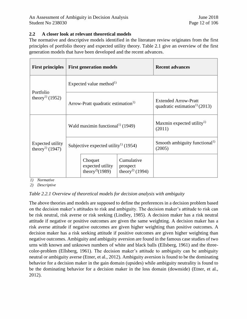
The normative and descriptive models identified in the literature review originates from the first
principles of portfolio theory and expected utility theory. Table 2.1 give an overview of the first
generation models that have been developed and the recent advances.
First principles
First generation models
Recent advances
Portfolio
theory1) (1952)
Expected value method1)
Arrow-Pratt quadratic estimation1)
Extended Arrow-Pratt
quadratic estimation1) (2013)
Expected utility
theory1) (1947)
Wald maximin functional1) (1949)
Maxmin expected utility1)
(2011)
Subjective expected utility1) (1954)
Smooth ambiguity functional1)
(2005)
Choquet
expected utility
theory2)(1989)
Cumulative
prospect
theory2) (1994)
1) Normative
2) Descriptive
Table 2.2.1 Overview of theoretical models for decision analysis with ambiguity
The above theories and models are supposed to define the preferences in a decision problem based
on the decision maker’s attitudes to risk and ambiguity. The decision maker’s attitude to risk can
be risk neutral, risk averse or risk seeking (Lindley, 1985). A decision maker has a risk neutral
attitude if negative or positive outcomes are given the same weighting. A decision maker has a
risk averse attitude if negative outcomes are given higher weighting than positive outcomes. A
decision maker has a risk seeking attitude if positive outcomes are given higher weighting than
negative outcomes. Ambiguity and ambiguity aversion are found in the famous case studies of two
urns with known and unknown numbers of white and black balls (Ellsberg, 1961) and the three-
color-problem (Ellsberg, 1961). The decision maker’s attitude to ambiguity can be ambiguity
neutral or ambiguity averse (Etner, et al., 2012). Ambiguity aversion is found to be the dominating
behavior for a decision maker in the gain domain (upsides) while ambiguity neutrality is found to
be the dominating behavior for a decision maker in the loss domain (downside) (Etner, et al.,
2012).
An Assessment of Ambiguity in Decision Analysis June 2018
Student No 238030 Page 13 of 106
The expected value method is derived from the normative portfolio theory (Markowitz, 1952) and
represents a linear combination of payoffs and probabilities. The expected value method is
considered to be a risk neutral approach. The expected utility theory (von Neumann &
Morgenstern, 1947) is a value representation that can include aversion to risk or loss by a utility
function. A rational decision maker is then supposed to maximize the expected utility by a linear
combination of utilities and lotteries described by objective probabilities. The expected utility is a
normative theory which means that it gives a prescription of a rational decision maker. Subjective
expected utility (Savage, 1954) is a further development of expected utility theory where the
lotteries are redefined as acts and the objective probabilities are redefined as subjective
probabilities. A rational decision maker is, in the framework of subjective expected utility, also
maximizing expected utility as a linear combination of utilities and probabilities, and can also have
utility functions that includes aversion to risk. The subjective expected utility is considered to be
an ambiguity neutral approach (Etner, et al., 2012). The preferences to an extreme risk and
ambiguity averse or maxmin decision maker is the minimum of the worst consequences of an
outcome set (Wald, 1949). The maxmin expected utility (Gilboa & Schmeidler, 1989) is a further
generalization of the Wald maximin criterion. Maxmin expected utility is based on multiple priors
for the outcome set where the decision maker will make his preferences by comparing the minimal
expected utility of two decision alternatives (Etner, et al., 2012). The Extended Arrow-Pratt
Quadratic Estimation method (Maccheroni, et al., 2013) is based on the portfolio theory of mean,
variance and covariance and introduce parameters for risk aversion and ambiguity aversion. The
Smooth Ambiguity Functional (Klibanoff, et al., 2005) is a further development of the subjective
expected utility theory, where the ambiguity aversion is introduced as a second order function of
the utility function. The Choquet Expected Utility theory (Schmeidler, 1989) (Mangelsdorff &
Weber, 1994) is an extension to subjective expected utility theory that is based on non-additive
probabilities. The Choquet Expected Utility theory is a descriptive theory that cover situations
where the outcomes are only negative or only positive. The cumulative prospect theory (Kahneman
& Tversky, 1992) is based on the descriptive Choquet Expected Utility theory. The cumulative
prospect theory describes how a person makes his choice based on his individual reference point
and attitude towards loss and gain.
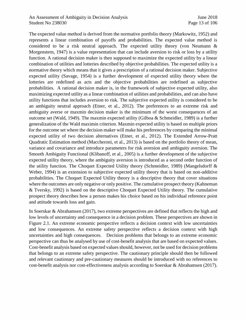
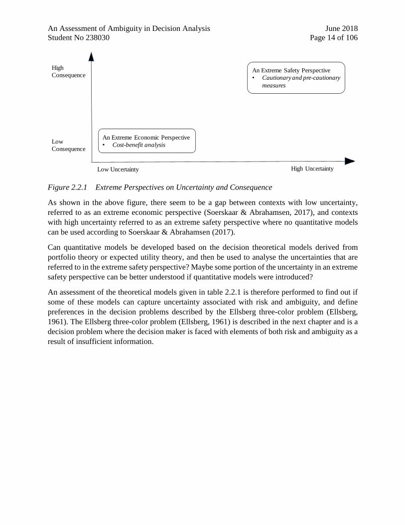
In Soerskar & Abrahamsen (2017), two extreme perspectives are defined that reflects the high and
low levels of uncertainty and consequence in a decision problem. These perspectives are shown in
Figure 2.1. An extreme economic perspective reflects a decision context with low uncertainties
and low consequences. An extreme safety perspective reflects a decision context with high
uncertainties and high consequences. Decision problems that belongs to an extreme economic
perspective can thus be analysed by use of cost-benefit analysis that are based on expected values.
Cost-benefit analysis based on expected values should, however, not be used for decision problems
that belongs to an extreme safety perspective. The cautionary principle should then be followed
and relevant cautionary and pre-cautionary measures should be introduced with no references to
cost-benefit analysis nor cost-effectiveness analysis according to Soerskar & Abrahamsen (2017).
An Assessment of Ambiguity in Decision Analysis June 2018
Student No 238030 Page 14 of 106
Figure 2.2.1 Extreme Perspectives on Uncertainty and Consequence
As shown in the above figure, there seem to be a gap between contexts with low uncertainty,
referred to as an extreme economic perspective (Soerskaar & Abrahamsen, 2017), and contexts
with high uncertainty referred to as an extreme safety perspective where no quantitative models
can be used according to Soerskaar & Abrahamsen (2017).
Can quantitative models be developed based on the decision theoretical models derived from
portfolio theory or expected utility theory, and then be used to analyse the uncertainties that are
referred to in the extreme safety perspective? Maybe some portion of the uncertainty in an extreme
safety perspective can be better understood if quantitative models were introduced?
An assessment of the theoretical models given in table 2.2.1 is therefore performed to find out if
some of these models can capture uncertainty associated with risk and ambiguity, and define
preferences in the decision problems described by the Ellsberg three-color problem (Ellsberg,
1961). The Ellsberg three-color problem (Ellsberg, 1961) is described in the next chapter and is a
decision problem where the decision maker is faced with elements of both risk and ambiguity as a
result of insufficient information.
High
Consequence
Low
Consequence
High UncertaintyLow Uncertainty
An Extreme Safety Perspective
• Cautionary and pre-cautionary
measures
An Extreme Economic Perspective
• Cost-benefit analysis
An Assessment of Ambiguity in Decision Analysis June 2018
Student No 238030 Page 15 of 106
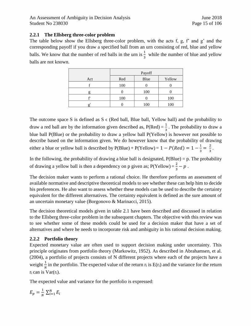
2.2.1 The Ellsberg three-color problem
The table below show the Ellsberg three-color problem, with the acts f, g, f’ and g’ and the
corresponding payoff if you draw a specified ball from an urn consisting of red, blue and yellow
balls. We know that the number of red balls in the urn is 1
3 while the number of blue and yellow
balls are not known.
Act
Payoff
Red Blue Yellow
f 100 0 0
g 0 100 0
f' 100 0 100
g' 0 100 100
The outcome space S is defined as S ϵ (Red ball, Blue ball, Yellow ball) and the probability to
draw a red ball are by the information given described as, P(Red) = 1
3 . The probability to draw a
blue ball P(Blue) or the probability to draw a yellow ball P(Yellow) is however not possible to
describe based on the information given. We do however know that the probability of drawing
either a blue or yellow ball is described by P(Blue) + P(Yellow) = 1 − 𝑃(𝑅𝑒𝑑) = 1 −1
3=
2
3 .
In the following, the probability of drawing a blue ball is designated, P(Blue) = p. The probability
of drawing a yellow ball is then a dependency on p given as; P(Yellow) = 2
3− 𝑝 .
The decision maker wants to perform a rational choice. He therefore performs an assessment of
available normative and descriptive theoretical models to see whether these can help him to decide
his preferences. He also want to assess whether these models can be used to describe the certainty
equivalent for the different alternatives. The certainty equivalent is defined as the sure amount of
an uncertain monetary value (Borgonovo & Marinacci, 2015).
The decision theoretical models given in table 2.1 have been described and discussed in relation
to the Ellsberg three-color problem in the subsequent chapters. The objective with this review was
to see whether some of these models could be used for a decision maker that have a set of
alternatives and where he needs to incorporate risk and ambiguity in his rational decision making.
2.2.2 Portfolio theory
Expected monetary value are often used to support decision making under uncertainty. This
principle originates from portfolio theory (Markowitz, 1952). As described in Abrahamsen, et al.
(2004), a portfolio of projects consists of N different projects where each of the projects have a
weight 1
𝑁 in the portfolio. The expected value of the return ri is E(ri) and the variance for the return
ri can is Var(ri).
The expected value and variance for the portfolio is expressed:
𝐸𝑝 =1
𝑁 ∑ 𝐸𝑖
𝑁𝑖=1
An Assessment of Ambiguity in Decision Analysis June 2018
Student No 238030 Page 16 of 106
The variance for the portfolio is expressed:
𝑉𝐴𝑅𝑝 = ∑ (1
𝑁)2𝑉𝐴𝑅𝑖
𝑁
𝑖=1+ ∑ ∑ (
1
𝑁)2𝐶𝑂𝑉𝑖,𝑗
𝑁
𝑗ǂ𝑖,𝑗=1
𝑁
𝑖=1
= 1
𝑁 𝑉𝐴𝑅 + (1 −
1
𝑁)𝐶𝑂𝑉
Where;
𝐶𝑂𝑉𝑖,𝑗 = 𝐸{(𝑟𝑖 − 𝐸𝑖) ∙ (𝑟𝑗 − 𝐸𝑗)}
𝑉𝐴𝑅 =1
𝑁 ∑ 𝑉𝐴𝑅𝑖
𝑁𝑖=1 .
𝐶𝑂𝑉 =1
𝑁2−𝑁 ∑ ∑ 𝐶𝑂𝑉𝑖,𝑗
𝑁
𝑗ǂ𝑖,𝑗=1
𝑁
𝑖=1
The unsystematic risk which refers to specific project uncertainties is in the above described by
the average variance 𝑉𝐴𝑅 and the systematic risk which refers to general market movements is in
the above described by the average covariance 𝐶𝑂𝑉. In a portfolio with a large number of projects,
we then see that the systematic risk represented by the average covariance will dominate since the
average variance will go to zero when N is large.
The project portfolio perspective is therefore relevant when assessing the risk and return for a
company with several projects. For a single project however, the unsystematic risk will dominate
and the expected values can have large deviations from the true values.
A broader perspective than the expected values is therefore needed in order to take account of
uncertainties. To calculate the expected monetary values is however a very common method to
use in decision analysis. The problem with this method is that positive and negative outcomes are
given the same weight and that the decision maker therefore is neutral to a potential negative or
positive outcome. This is commonly termed as being risk neutral.
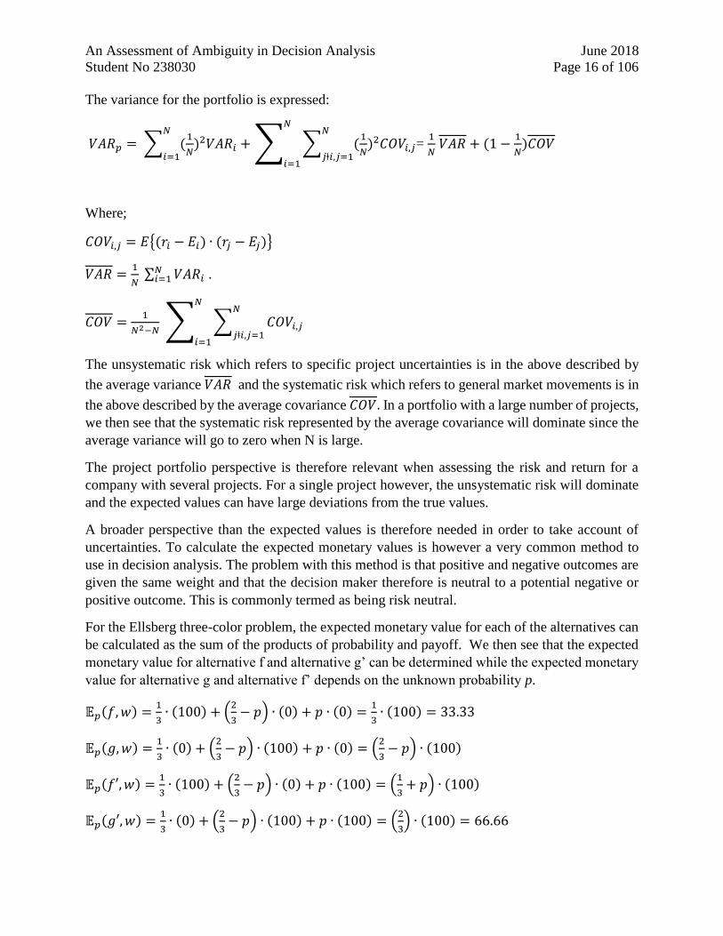
For the Ellsberg three-color problem, the expected monetary value for each of the alternatives can
be calculated as the sum of the products of probability and payoff. We then see that the expected
monetary value for alternative f and alternative g’ can be determined while the expected monetary
value for alternative g and alternative f’ depends on the unknown probability p.
𝔼𝑝(𝑓, 𝑤) =1
3∙ (100) + (
2
3− 𝑝) ∙ (0) + 𝑝 ∙ (0) =
1
3∙ (100) = 33.33
𝔼𝑝(𝑔, 𝑤) =1
3∙ (0) + (
2
3− 𝑝) ∙ (100) + 𝑝 ∙ (0) = (
2
3− 𝑝) ∙ (100)
𝔼𝑝(𝑓′, 𝑤) =1
3∙ (100) + (
2
3− 𝑝) ∙ (0) + 𝑝 ∙ (100) = (
1
3+ 𝑝) ∙ (100)
𝔼𝑝(𝑔′, 𝑤) =1
3∙ (0) + (
2
3− 𝑝) ∙ (100) + 𝑝 ∙ (100) = (
2
3) ∙ (100) = 66.66
An Assessment of Ambiguity in Decision Analysis June 2018
Student No 238030 Page 17 of 106
The expected monetary value for option g and f’ will vary depending on the probability value of p
which could range between 0 and 2
3 . If p is close to
2
3 , then option f’ will have the maximum
expected value. If p is close to 0 , then option g and option g’ will have the maximum expected
value. The preferred option in the Ellsberg three-color problem is therefore not possible to decide
for the decision maker based on the principle of expected monetary value since the probability p
is non-uniquely defined.
2.2.3 Expected utility theory
The expected utility theory assumes that a decision maker’s choice and behavior is based on
rational decision making. A set of axioms were defined by von Neumann and Morgenstern (1947)
that defined the rational behavior and the decision maker’s preference over lotteries (Abrahamsen
& Aven, 2008). A lottery can be described as a set of outcomes where the probability of occurrence
for each of the outcomes can be described by objective probabilities. Lotteries are defined in a
state space S = {𝑋, 𝑌, 𝑍} where the decision maker may have a preference over lotteries X, Y and
Z. The “Weak order” axiom defines the decision maker’s preference over lotteries based on the
properties of completeness, transitive and reflexive. Completeness means that the decision maker
can prefer X over Y, or Y over X or can be indifferent between X and Y. Transitive means that the
decision maker prefer X over Y and Y over Z, it is also then given that the decision maker prefers
X over Z. Reflexive means that the decision maker is indifferent between two identical lotteries X
and X. The “Continuity” axiom defines that there exists only one value of p between 0 and 1 which
makes the decision maker indifferent between lottery Y and a compound lottery of X and Z, this
implies that Y~ pX + (1-p)Z. The “Preference increasing with probability” axiom means that a
decision maker preference of two lotteries X and Y with the same outcomes would be the lottery
with the highest probability. The “Compound probabilities” axiom defines that any lottery which
has further lotteries as outcomes can be reduced to a one stage lottery. The “independence” axiom
states that if a decision maker has a preference to lottery X over lottery Y this preference should
not change if a common outcome in both lotteries are changed.
The important feature of utility theory is that the utility value function can have a shape that
represents the decision maker’s attitude or weighting to gain and loss. The utility can be defined
as a linear function or in a concave or convex shape. If the utility function is linear the decision
maker is neutral, which means that a negative or positive outcome are given the same weighting.
If the utility function has a concave shape this means that negative outcomes are given higher
weighting than the positive outcomes. If the utility function has a convex shape, this means that
the positive outcomes are given higher weighting than the negative outcomes.
If we have a defined state space S = {𝑋, 𝑌, 𝑍} and have defined the utilities and the probabilities of
occurrence for the outcome space, then the expected utility is found as a linear combination of the
utilities and the corresponding probabilities. The rational decision maker will then have a
preference for the lottery that maximizes his expected utility.
The state space for the Ellsberg three-color problem is however not lotteries where the success of
all outcomes are described by objective probabilities. An objective probability for red balls exists
but not objective probabilities for the blue balls and respectively for yellow balls, only for their
An Assessment of Ambiguity in Decision Analysis June 2018
Student No 238030 Page 18 of 106
union. The basis for the use of the expected utility is therefore not satisfied for the Ellsberg three-
color problem and the decision maker is not able to perform a rational choice of his preferences
by the use of expected utility.
2.2.4 Subjective expected utility theory
Savage (1954) described the subjective expected utility (SEU) as a function of the subjective
probabilities defined by Ramsey (1931) and de Finetti and the expected utility as defined by von
Neumann and Morgenstern (1947). Several postulates were defined by Savage (1954) that
represents a further refinement of the axioms defined for expected utility by von Neumann and
Morgenstern. The most important postulate is the sure-thing principle, which refer back to the
“independence” axiom. Another important postulate by Savage (1954) relate to the preference of
an outcome space, which means that if the outcome space {0, 100} is changed to {0, 1000} this
should not result in change in preference.
Savage also changed the state space from a set of lotteries to a set of acts which could include
lotteries but also other actions where the subjective belief of the decision maker is described by
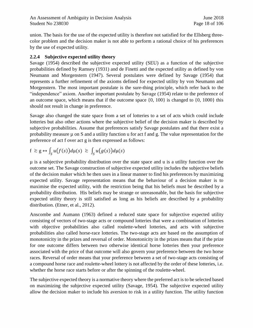
subjective probabilities. Assume that preferences satisfy Savage postulates and that there exist a
probability measure µ on S and a utility function u for act f and g. The value representation for the
preference of act f over act g is then expressed as follows:
f ≿ g ↔ ∫ 𝑢(𝑓(𝑠))𝑑µ(𝑠𝑆
) ≿ ∫ 𝑢(𝑔(𝑠))𝑑µ(𝑠𝑆
)
µ is a subjective probability distribution over the state space and u is a utility function over the
outcome set. The Savage construction of subjective expected utility includes the subjective beliefs
of the decision maker which he then uses in a linear manner to find his preferences by maximizing
expected utility. Savage representation means that the behaviour of a decision maker is to
maximise the expected utility, with the restriction being that his beliefs must be described by a
probability distribution. His beliefs may be strange or unreasonable, but the basis for subjective
expected utility theory is still satisfied as long as his beliefs are described by a probability
distribution. (Etner, et al., 2012).
Anscombe and Aumann (1963) defined a reduced state space for subjective expected utility
consisting of vectors of two-stage acts or compound lotteries that were a combination of lotteries
with objective probabilities also called roulette-wheel lotteries, and acts with subjective
probabilities also called horse-race lotteries. The two-stage acts are based on the assumption of
monotonicity in the prizes and reversal of order. Monotonicity in the prizes means that if the prize
for one outcome differs between two otherwise identical horse lotteries then your preference
associated with the price of that outcome will also govern your preference between the two horse
races. Reversal of order means that your preference between a set of two-stage acts consisting of
a compound horse race and roulette-wheel lottery is not affected by the order of these lotteries, i.e.
whether the horse race starts before or after the spinning of the roulette-wheel.
The subjective expected theory is a normative theory where the preferred act is to be selected based
on maximizing the subjective expected utility (Savage, 1954). The subjective expected utility
allow the decision maker to include his aversion to risk in a utility function. The utility function
An Assessment of Ambiguity in Decision Analysis June 2018
Student No 238030 Page 19 of 106
for risk aversion is normally described as a concave exponential function where the negative
payoffs are given a much higher weight than a positive payoff and where a high payoff is reduced
in relation to a lower payoff.
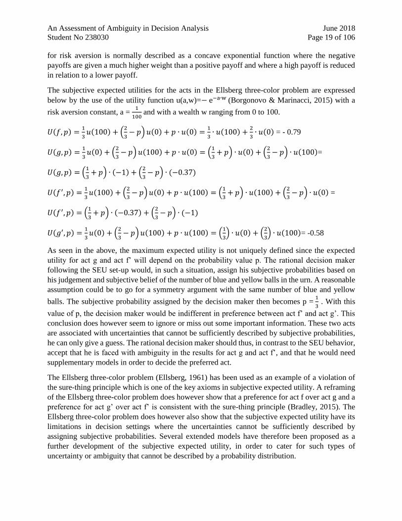
The subjective expected utilities for the acts in the Ellsberg three-color problem are expressed
below by the use of the utility function u(a,w)=− e−a∙w (Borgonovo & Marinacci, 2015) with a
risk aversion constant, a = 1
100 and with a wealth w ranging from 0 to 100.
𝑈(𝑓, 𝑝) =1
3𝑢(100) + (
2
3− 𝑝) 𝑢(0) + 𝑝 ∙ 𝑢(0) =
1
3∙ 𝑢(100) +
2
3∙ 𝑢(0) = - 0.79
𝑈(𝑔, 𝑝) =1
3𝑢(0) + (
2
3− 𝑝) 𝑢(100) + 𝑝 ∙ 𝑢(0) = (
1
3+ 𝑝) ∙ 𝑢(0) + (
2
3− 𝑝) ∙ 𝑢(100)=
𝑈(𝑔, 𝑝) = (1
3+ 𝑝) ∙ (−1) + (
2
3− 𝑝) ∙ (−0.37)
𝑈(𝑓′, 𝑝) =1
3𝑢(100) + (
2
3− 𝑝) 𝑢(0) + 𝑝 ∙ 𝑢(100) = (
1
3+ 𝑝) ∙ 𝑢(100) + (
2
3− 𝑝) ∙ 𝑢(0) =
𝑈(𝑓′, 𝑝) = (1
3+ 𝑝) ∙ (−0.37) + (
2
3− 𝑝) ∙ (−1)
𝑈(𝑔′, 𝑝) =1
3𝑢(0) + (
2
3− 𝑝) 𝑢(100) + 𝑝 ∙ 𝑢(100) = (
1
3) ∙ 𝑢(0) + (
2
3) ∙ 𝑢(100)= -0.58
As seen in the above, the maximum expected utility is not uniquely defined since the expected
utility for act g and act f’ will depend on the probability value p. The rational decision maker
following the SEU set-up would, in such a situation, assign his subjective probabilities based on
his judgement and subjective belief of the number of blue and yellow balls in the urn. A reasonable
assumption could be to go for a symmetry argument with the same number of blue and yellow
balls. The subjective probability assigned by the decision maker then becomes p = 1
3 . With this
value of p, the decision maker would be indifferent in preference between act f’ and act g’. This
conclusion does however seem to ignore or miss out some important information. These two acts
are associated with uncertainties that cannot be sufficiently described by subjective probabilities,
he can only give a guess. The rational decision maker should thus, in contrast to the SEU behavior,
accept that he is faced with ambiguity in the results for act g and act f’, and that he would need
supplementary models in order to decide the preferred act.
The Ellsberg three-color problem (Ellsberg, 1961) has been used as an example of a violation of
the sure-thing principle which is one of the key axioms in subjective expected utility. A reframing
of the Ellsberg three-color problem does however show that a preference for act f over act g and a
preference for act g’ over act f’ is consistent with the sure-thing principle (Bradley, 2015). The
Ellsberg three-color problem does however also show that the subjective expected utility have its
limitations in decision settings where the uncertainties cannot be sufficiently described by
assigning subjective probabilities. Several extended models have therefore been proposed as a
further development of the subjective expected utility, in order to cater for such types of
uncertainty or ambiguity that cannot be described by a probability distribution.
An Assessment of Ambiguity in Decision Analysis June 2018
Student No 238030 Page 20 of 106
2.2.5 Wald maximin functional
The Wald maximin criterion (Wald, 1949), (Gilboa & Marinacci, 2011), (Etner, et al., 2012) is a
very conservative model where preference is based exclusively by the worst possible
consequences. If the outcome set is {𝑥, 𝑦, 𝑧} where x represent the worst consequence, then the
decision maker would make his preference based on u(x) from this outcome set. (Etner, et al.,
2012).
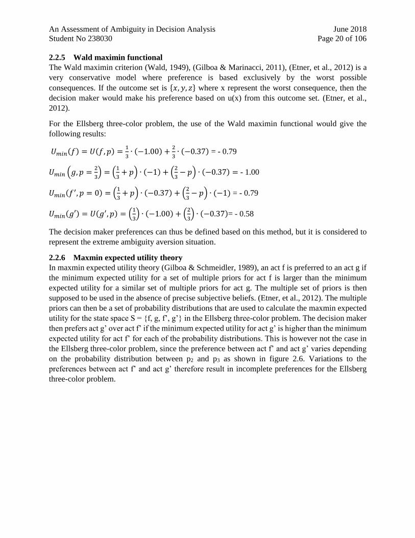
For the Ellsberg three-color problem, the use of the Wald maximin functional would give the
following results:
𝑈𝑚𝑖𝑛(𝑓) = 𝑈(𝑓, 𝑝) =1
3∙ (−1.00) +
2
3∙ (−0.37) = - 0.79
𝑈𝑚𝑖𝑛 (𝑔, 𝑝 =2
3) = (
1
3+ 𝑝) ∙ (−1) + (
2
3− 𝑝) ∙ (−0.37) = - 1.00
𝑈𝑚𝑖𝑛(𝑓′, 𝑝 = 0) = (1
3+ 𝑝) ∙ (−0.37) + (
2
3− 𝑝) ∙ (−1) = - 0.79
𝑈𝑚𝑖𝑛(𝑔′) = 𝑈(𝑔′, 𝑝) = (1
3) ∙ (−1.00) + (
2
3) ∙ (−0.37)= - 0.58
The decision maker preferences can thus be defined based on this method, but it is considered to
represent the extreme ambiguity aversion situation.
2.2.6 Maxmin expected utility theory
In maxmin expected utility theory (Gilboa & Schmeidler, 1989), an act f is preferred to an act g if
the minimum expected utility for a set of multiple priors for act f is larger than the minimum
expected utility for a similar set of multiple priors for act g. The multiple set of priors is then
supposed to be used in the absence of precise subjective beliefs. (Etner, et al., 2012). The multiple
priors can then be a set of probability distributions that are used to calculate the maxmin expected
utility for the state space S = {f, g, f’, g’} in the Ellsberg three-color problem. The decision maker
then prefers act g’ over act f’ if the minimum expected utility for act g’ is higher than the minimum
expected utility for act f’ for each of the probability distributions. This is however not the case in
the Ellsberg three-color problem, since the preference between act f’ and act g’ varies depending
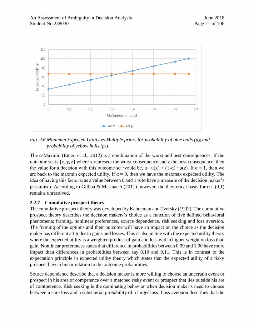
on the probability distribution between p2 and p3 as shown in figure 2.6. Variations to the
preferences between act f’ and act g’ therefore result in incomplete preferences for the Ellsberg
three-color problem.
An Assessment of Ambiguity in Decision Analysis June 2018
Student No 238030 Page 21 of 106
Fig. 2.6 Minimum Expected Utility vs Multiple priors for probability of blue balls (p2) and
probability of yellow balls (p3)
The α-Maxmin (Etner, et al., 2012) is a combination of the worst and best consequences. If the
outcome set is {𝑥, 𝑦, 𝑧} where x represent the worst consequence and z the best consequence, then
the value for a decision with this outcome set would be, α ∙ u(x) + (1-α) ∙ u(z). If α = 1, then we
are back to the maxmin expected utility. If α = 0, then we have the maxmax expected utility. The
idea of having this factor α as a value between 0 and 1 is to have a measure of the decision maker’s
pessimism. According to Gilboa & Marinacci (2011) however, the theoretical basis for α ϵ (0,1)
remains unresolved.
2.2.7 Cumulative prospect theory
The cumulative prospect theory was developed by Kahneman and Tversky (1992). The cumulative
prospect theory describes the decision makers’s choice as a function of five defined behavioral
phenomena; framing, nonlinear preferences, source dependence, risk seeking and loss aversion.
The framing of the options and their outcome will have an impact on the choice as the decision
maker has different attitudes to gains and losses. This is also in line with the expected utility theory
where the expected utility is a weighted product of gain and loss with a higher weight on loss than
gain. Nonlinear preferences states that difference in probabilities between 0.99 and 1.00 have more
impact than differences in probabilities between say 0.10 and 0.11. This is in contrast to the
expectation principle in expected utility theory which states that the expected utility of a risky
prospect have a linear relation to the outcome probabilities.
Source dependence describe that a decision maker is more willing to choose an uncertain event or
prospect in his area of competence over a matched risky event or prospect that lies outside his are
of comtpetence. Risk seeking is the dominating behavior when decision maker’s need to choose
between a sure loss and a substantial probability of a larger loss. Loss aversion describes that the
0
20
40
60
80
100
120
0 0.1 0.2 0.3 0.4 0.5 0.6 0.7
Ex
pe
cte
d U
tilt
ity
Multiple prior for p3
Expected Utility vs Multiple priors for p3
Act f' Act g'
An Assessment of Ambiguity in Decision Analysis June 2018
Student No 238030 Page 22 of 106
decision maker is found to be more sensitive to losses than to gains. The loss aversion, risk seeking
and nonlinear preferences are in cumulative prospect theory represented by a value and weighting
function. The value of each outcome are separated for gains and losses and these are then
multiplied by non-additive decision weights, which is different from gains and losses.
The cumulative prospect theory (Kahneman & Tversky, 1992) is a further development of rank
dependent utility also called Choquet expected utility (Etner, et al., 2012). Choquet expected utility
(Schmeidler, 1989) is then again a further development of the subjective expected theory, but
where the beliefs of the decision maker are not described by non-additive probabilities, also
described as non-additive capacities. An act f is then preferred to an act g if there exists a utility
function u and a capacity v that satisfies the following utility value representations:
∫ 𝑢(𝑓)𝑑𝑣 ≥ ∫ 𝑢(𝑔)𝑑𝑣𝐶ℎ𝐶ℎ
With the outcome space S={𝑠1, 𝑠2, … . , 𝑠𝑛}, the Choquet integral is further defined by:
∫ 𝑢(𝑓)𝑑𝑣 ≥ 𝑢(𝑥1) +𝐶ℎ
(𝑢(𝑥2) − 𝑢(𝑥1)) ∙ 𝑣({𝑠2, 𝑠3, … . , 𝑠𝑛}) + ⋯ + (𝑢(𝑥𝑖+1) − 𝑢(𝑥𝑖))
∙ 𝑣({𝑠𝑖+1, … . , 𝑠𝑛}) + ⋯ + (𝑢(𝑥𝑛) − 𝑢(𝑥𝑛−1)) ∙ 𝑣({𝑠𝑛})
The Choquet integral consider first the lowest outcome and then add the positive increments that
are weighted with decision maker’s belief represented by the capacities v(s) over the outcome
space S.
The cumulative prospect theory (Kahneman & Tversky, 1992) also uses capacities to describe the
decision maker’s beliefs. The difference between Choquet expected utility and cumulative
prospect theory is however that the latter has one set of capacities for gains, and another set of
capacities for losses. The utility value representation in cumulative prospect theory for an act f is
then described by a utility function u and a capacity for gain v+ and for loss v- as follows:
𝑉(𝑓) = 𝑢(𝑥1) + ∑ 𝑣−(𝑈𝑗=1𝑘
𝑘
𝑖=2
{𝑠𝑗})(𝑢(𝑥𝑖) − 𝑢(𝑥𝑖−1)) + ∑ 𝑣+(𝑈𝑗=1𝑘
𝑘
𝑖=𝑘+1
{𝑠𝑗})(𝑢(𝑥𝑖) − 𝑢(𝑥𝑖−1))
An issue with the cumulative prospect theory is that the model supposes that there is a reference
point where the decision maker treats outcomes above as gains and outcomes below as losses.
In the Ellsberg three-color problem, the reference point for the decision maker is 0 since there are
only outcomes with a gain of 0 or 100. The negative portion of the value representation for the
cumulative prospect theory is therefore not relevant and the cumulative prospect theory value
representation is reduced to a Choquet value representation. In Mangelsdorff & Weber (1994), the
Ellsberg three-color problem has been assessed by the use of Choquet expected utility. The
Choquet expected utility is here used to formulate a value representation of the prospects based on
the decision maker’s initial preferences, or by empirical surveys.
An Assessment of Ambiguity in Decision Analysis June 2018
Student No 238030 Page 23 of 106
2.2.8 Extended Arrow-Pratt Quadratic Estimation
The certainty equivalent for an expected utility maximizer with utility u, wealth w and investment
h can be expressed by the Arrow-Pratt approximation (Maccheroni, et al., 2013) given by:
𝑐(𝑤 + ℎ, 𝑃) ≈ 𝑤 + 𝐸𝑃(ℎ) −1
2𝜆𝑢(𝑤)𝜎𝑝
2(ℎ)
𝐸𝑃(ℎ) is the expected wealth of the investment h based on the probabilistic model P. 𝜎𝑝2(ℎ) is the
statistical variation of the investment h with respect to the probabilistic model P. The coefficient
𝜆𝑢(𝑤) = − 𝑢′′(𝑤)
𝑢′(𝑤) which is the ratio between the double derivative and the derivative of the u
function, describe the agent’s or decision maker’s aversion to risk.
By setting f = w + h and 𝜆 = 𝜆𝑢(𝑤), the value representation or certainty equivalent for a prospect
f becomes:
𝐶(𝑓) = 𝐸𝑃(𝑓) −𝜆
2𝜎𝑝
2(𝑓)
The risk premium for prospect f is therefore given by:
П𝜆 = 𝜆
2𝜎𝑝
2(𝑓)
A premium for ambiguity for prospect f can further be found by quadratic approximation of an
extension to the Arrow-Pratt analysis to account for model uncertainty (Maccheroni, et al., 2013).
Model uncertainty then refers to situations where the decision maker is uncertain about the
probabilistic model P.
The quadratic approximation takes an exact form as given below if the investment h has a normal
cumulative distribution 𝜑(∙; 𝑚, 𝜎) with unknown mean m and known variance 𝜎2 (Maccheroni, et
al., 2013). It is also then supposed that the prior on the unknown means m is given by a normal
cumulative distribution 𝜑(∙; µ, 𝜎). Due to the normal distribution of the prior, this implies that µ
is the mean of the unknown means m and 𝜎µ2 is the variance of the unknown means.
C(w + h) = 𝑣−1(∫ 𝑣 (𝑢−1(∫ 𝑢(𝑤 + 𝑥)𝑑𝜑(𝑚; µ , 𝜎µ))
= 𝑣−1(∫ 𝑣 (𝑢−1(𝑤 + 𝑚 −1
2𝜆𝑢(𝑤) ∙ 𝜎2)𝑑𝜑(𝑚; µ , 𝜎µ))
= 𝑤 + µ −1
2𝜆𝑢(𝑤)𝜎2 −
1
2𝜆𝑣(𝑤)𝜎µ
2
The standard mean-variance quadratic approximation or certainty equivalent to account for model
uncertainty or ambiguity is given below and are determined by the parameters, λ, ɵ and µ at a
constant w such that λ = 𝜆𝑢(𝑤) and ɵ = 𝜆𝑣(𝑤) − 𝜆𝑢(𝑤). The parameters λ and ɵ represents the
decision maker’s negative attitude towards risk (λ) and ambiguity (ɵ). 𝜎µ2(𝐸(𝑓)) is the variance of
the averages of prospect f or the variance of the expected value of prospect f.
𝐶(𝑓) = 𝐸𝑃(𝑓) −𝜆
2𝜎𝑃
2(𝑓) −ɵ
2𝜎µ
2(𝐸(𝑓))
An Assessment of Ambiguity in Decision Analysis June 2018
Student No 238030 Page 24 of 106
The ambiguity premium for the prospect f is therefore given by:
Пɵ = ɵ
2𝜎µ
2(𝐸(𝑓))
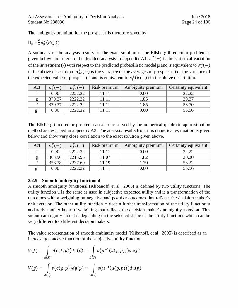
A summary of the analysis results for the exact solution of the Ellsberg three-color problem is
given below and refers to the detailed analysis in appendix A1. 𝜎µ2(−) is the statistical variation
of the investment (-) with respect to the predicted probabilistic model µ and is equivalent to 𝜎𝑝2(−)
in the above description. 𝜎𝐴𝑃2 (−) is the variance of the averages of prospect (-) or the variance of
the expected value of prospect (-) and is equivalent to 𝜎µ2(𝐸(−)) in the above description.
Act 𝜎µ2(−) 𝜎𝐴𝑃
2 (−) Risk premium Ambiguity premium Certainty equivalent
f 0.00 2222.22 11.11 0.00 22.22
g 370.37 2222.22 11.11 1.85 20.37
f’ 370.37 2222.22 11.11 1.85 53.70
g’ 0.00 2222.22 11.11 0.00 55.56
The Ellsberg three-color problem can also be solved by the numerical quadratic approximation
method as described in appendix A2. The analysis results from this numerical estimation is given
below and show very close correlation to the exact solution given above.
Act 𝜎µ2(−) 𝜎𝐴𝑃
2 (−) Risk premium Ambiguity premium Certainty equivalent
f 0.00 2222.22 11.11 0.00 22.22
g 363.96 2213.95 11.07 1.82 20.20
f’ 358.28 2237.69 11.19 1.79 53.22
g’ 0.00 2222.22 11.11 0.00 55.56
2.2.9 Smooth ambiguity functional
A smooth ambiguity functional (Klibanoff, et al., 2005) is defined by two utility functions. The
utility function u is the same as used in subjective expected utility and is a transformation of the
outcomes with a weighting on negative and positive outcomes that reflects the decision maker’s
risk aversion. The other utility function φ does a further transformation of the utility function u
and adds another layer of weighting that reflects the decision maker’s ambiguity aversion. This
smooth ambiguity model is depending on the selected shape of the utility functions which can be
very different for different decision makers.
The value representation of smooth ambiguity model (Klibanoff, et al., 2005) is described as an
increasing concave function of the subjective utility function.
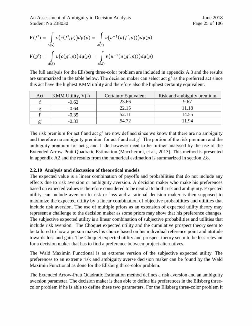
𝑉(𝑓) = ∫ 𝑣(𝑐(𝑓, 𝑝))𝑑µ(𝑝)
𝛥(𝑆)
= ∫ 𝑣(𝑢−1(𝑢(𝑓, 𝑝)))𝑑µ(𝑝)
𝛥(𝑆)
𝑉(𝑔) = ∫ 𝑣(𝑐(𝑔, 𝑝))𝑑µ(𝑝)
𝛥(𝑆)
= ∫ 𝑣(𝑢−1(𝑢(𝑔, 𝑝)))𝑑µ(𝑝)
𝛥(𝑆)
An Assessment of Ambiguity in Decision Analysis June 2018
Student No 238030 Page 25 of 106
𝑉(𝑓′) = ∫ 𝑣(𝑐(𝑓′, 𝑝))𝑑µ(𝑝)
𝛥(𝑆)
= ∫ 𝑣(𝑢−1(𝑢(𝑓′, 𝑝)))𝑑µ(𝑝)
𝛥(𝑆)
𝑉(𝑔′) = ∫ 𝑣(𝑐(𝑔′, 𝑝))𝑑µ(𝑝)
𝛥(𝑆)
= ∫ 𝑣(𝑢−1(𝑢(𝑔′, 𝑝)))𝑑µ(𝑝)
𝛥(𝑆)
The full analysis for the Ellsberg three-color problem are included in appendix A.3 and the results
are summarized in the table below. The decision maker can select act g’ as the preferred act since
this act have the highest KMM utility and therefore also the highest certainty equivalent.
Act KMM Utility, V(-) Certainty Equivalent Risk and ambiguity premium
f -0.62 23.66 9.67
g -0.64 22.15 11.18
f' -0.35 52.11 14.55
g' -0.33 54.72 11.94
The risk premium for act f and act g’ are now defined since we know that there are no ambiguity
and therefore no ambiguity premium for act f and act g’. The portion of the risk premium and the
ambiguity premium for act g and f’ do however need to be further analysed by the use of the
Extended Arrow-Pratt Quadratic Estimation (Maccheroni, et al., 2013). This method is presented
in appendix A2 and the results from the numerical estimation is summarized in section 2.8.
2.2.10 Analysis and discussion of theoretical models
The expected value is a linear combination of payoffs and probabilities that do not include any
effects due to risk aversion or ambiguity aversion. A decision maker who make his preferences
based on expected values is therefore considered to be neutral to both risk and ambiguity. Expected
utility can include aversion to risk or loss and a rational decision maker is then supposed to
maximize the expected utility by a linear combination of objective probabilities and utilities that
include risk aversion. The use of multiple priors as an extension of expected utility theory may
represent a challenge to the decision maker as some priors may show that his preference changes.
The subjective expected utility is a linear combination of subjective probabilities and utilities that
include risk aversion. The Choquet expected utility and the cumulative prospect theory seem to
be tailored to how a person makes his choice based on his individual reference point and attitude
towards loss and gain. The Choquet expected utility and prospect theory seem to be less relevant
for a decision maker that has to find a preference between project alternatives.
The Wald Maximin Functional is an extreme version of the subjective expected utility. The
preferences to an extreme risk and ambiguity averse decision maker can be found by the Wald
Maximin Functional as done for the Ellsberg three-color problem.
The Extended Arrow-Pratt Quadratic Estimation method defines a risk aversion and an ambiguity
aversion parameter. The decision maker is then able to define his preferences in the Ellsberg three-
color problem if he is able to define these two parameters. For the Ellsberg three-color problem it
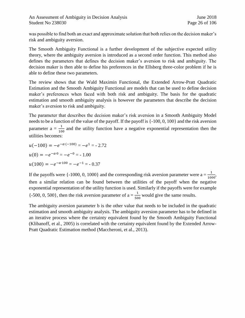
An Assessment of Ambiguity in Decision Analysis June 2018
Student No 238030 Page 26 of 106
was possible to find both an exact and approximate solution that both relies on the decision maker’s
risk and ambiguity aversion.
The Smooth Ambiguity Functional is a further development of the subjective expected utility
theory, where the ambiguity aversion is introduced as a second order function. This method also
defines the parameters that defines the decision maker’s aversion to risk and ambiguity. The
decision maker is then able to define his preferences in the Ellsberg three-color problem if he is
able to define these two parameters.
The review shows that the Wald Maximin Functional, the Extended Arrow-Pratt Quadratic
Estimation and the Smooth Ambiguity Functional are models that can be used to define decision
maker’s preferences when faced with both risk and ambiguity. The basis for the quadratic
estimation and smooth ambiguity analysis is however the parameters that describe the decision
maker’s aversion to risk and ambiguity.
The parameter that describes the decision maker’s risk aversion in a Smooth Ambiguity Model
needs to be a function of the value of the payoff. If the payoff is {-100, 0, 100} and the risk aversion
parameter a = 1
100 and the utility function have a negative exponential representation then the
utilities becomes:
𝑢(−100) = −𝑒−𝑎∙(−100) = −𝑒1 = - 2.72
𝑢(0) = −𝑒−𝑎∙0 = −𝑒−0 = - 1.00
𝑢(100) = −𝑒−𝑎∙100 = −𝑒−1 = - 0.37
If the payoffs were {-1000, 0, 1000} and the corresponding risk aversion parameter were a = 1
1000,
then a similar relation can be found between the utilities of the payoff when the negative
exponential representation of the utility function is used. Similarly if the payoffs were for example
{-500, 0, 500}, then the risk aversion parameter of a = 1
500 would give the same results.
The ambiguity aversion parameter b is the other value that needs to be included in the quadratic
estimation and smooth ambiguity analysis. The ambiguity aversion parameter has to be defined in
an iterative process where the certainty equivalent found by the Smooth Ambiguity Functional
(Klibanoff, et al., 2005) is correlated with the certainty equivalent found by the Extended Arrow-
Pratt Quadratic Estimation method (Maccheroni, et al., 2013).
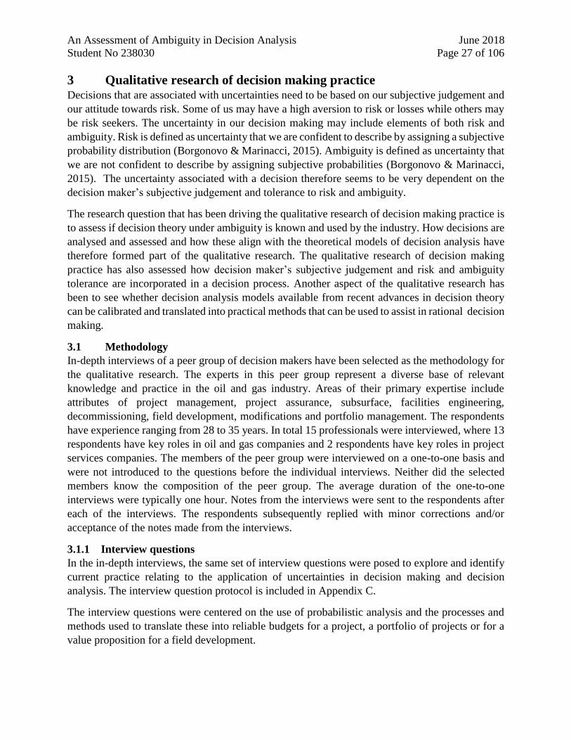
An Assessment of Ambiguity in Decision Analysis June 2018
Student No 238030 Page 27 of 106
3 Qualitative research of decision making practice Decisions that are associated with uncertainties need to be based on our subjective judgement and
our attitude towards risk. Some of us may have a high aversion to risk or losses while others may
be risk seekers. The uncertainty in our decision making may include elements of both risk and
ambiguity. Risk is defined as uncertainty that we are confident to describe by assigning a subjective
probability distribution (Borgonovo & Marinacci, 2015). Ambiguity is defined as uncertainty that
we are not confident to describe by assigning subjective probabilities (Borgonovo & Marinacci,
2015). The uncertainty associated with a decision therefore seems to be very dependent on the
decision maker’s subjective judgement and tolerance to risk and ambiguity.
The research question that has been driving the qualitative research of decision making practice is
to assess if decision theory under ambiguity is known and used by the industry. How decisions are
analysed and assessed and how these align with the theoretical models of decision analysis have
therefore formed part of the qualitative research. The qualitative research of decision making
practice has also assessed how decision maker’s subjective judgement and risk and ambiguity
tolerance are incorporated in a decision process. Another aspect of the qualitative research has
been to see whether decision analysis models available from recent advances in decision theory
can be calibrated and translated into practical methods that can be used to assist in rational decision
making.
3.1 Methodology
In-depth interviews of a peer group of decision makers have been selected as the methodology for
the qualitative research. The experts in this peer group represent a diverse base of relevant
knowledge and practice in the oil and gas industry. Areas of their primary expertise include
attributes of project management, project assurance, subsurface, facilities engineering,
decommissioning, field development, modifications and portfolio management. The respondents
have experience ranging from 28 to 35 years. In total 15 professionals were interviewed, where 13
respondents have key roles in oil and gas companies and 2 respondents have key roles in project
services companies. The members of the peer group were interviewed on a one-to-one basis and
were not introduced to the questions before the individual interviews. Neither did the selected
members know the composition of the peer group. The average duration of the one-to-one
interviews were typically one hour. Notes from the interviews were sent to the respondents after
each of the interviews. The respondents subsequently replied with minor corrections and/or
acceptance of the notes made from the interviews.
3.1.1 Interview questions
In the in-depth interviews, the same set of interview questions were posed to explore and identify
current practice relating to the application of uncertainties in decision making and decision
analysis. The interview question protocol is included in Appendix C.
The interview questions were centered on the use of probabilistic analysis and the processes and
methods used to translate these into reliable budgets for a project, a portfolio of projects or for a
value proposition for a field development.
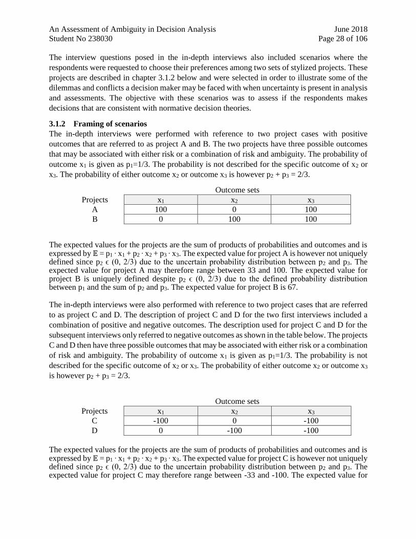
An Assessment of Ambiguity in Decision Analysis June 2018
Student No 238030 Page 28 of 106
The interview questions posed in the in-depth interviews also included scenarios where the
respondents were requested to choose their preferences among two sets of stylized projects. These
projects are described in chapter 3.1.2 below and were selected in order to illustrate some of the
dilemmas and conflicts a decision maker may be faced with when uncertainty is present in analysis
and assessments. The objective with these scenarios was to assess if the respondents makes
decisions that are consistent with normative decision theories.
3.1.2 Framing of scenarios
The in-depth interviews were performed with reference to two project cases with positive
outcomes that are referred to as project A and B. The two projects have three possible outcomes
that may be associated with either risk or a combination of risk and ambiguity. The probability of
outcome x1 is given as p1=1/3. The probability is not described for the specific outcome of x2 or
x3. The probability of either outcome x2 or outcome x3 is however p2 + p3 = 2/3.
Outcome sets
Projects x1 x2 x3
A 100 0 100
B 0 100 100
The expected values for the projects are the sum of products of probabilities and outcomes and is expressed by 𝔼 = p1 ∙ x1 + p2 ∙ x2 + p3 ∙ x3. The expected value for project A is however not uniquely defined since p2 ϵ (0, 2/3) due to the uncertain probability distribution between p2 and p3. The expected value for project A may therefore range between 33 and 100. The expected value for project B is uniquely defined despite p2 ϵ (0, 2/3) due to the defined probability distribution between p1 and the sum of p2 and p3. The expected value for project B is 67.
The in-depth interviews were also performed with reference to two project cases that are referred
to as project C and D. The description of project C and D for the two first interviews included a
combination of positive and negative outcomes. The description used for project C and D for the
subsequent interviews only referred to negative outcomes as shown in the table below. The projects
C and D then have three possible outcomes that may be associated with either risk or a combination
of risk and ambiguity. The probability of outcome x1 is given as p1=1/3. The probability is not
described for the specific outcome of x2 or x3. The probability of either outcome x2 or outcome x3
is however p2 + p3 = 2/3.
Outcome sets
Projects x1 x2 x3
C -100 0 -100
D 0 -100 -100
The expected values for the projects are the sum of products of probabilities and outcomes and is expressed by 𝔼 = p1 ∙ x1 + p2 ∙ x2 + p3 ∙ x3. The expected value for project C is however not uniquely defined since p2 ϵ (0, 2/3) due to the uncertain probability distribution between p2 and p3. The expected value for project C may therefore range between -33 and -100. The expected value for
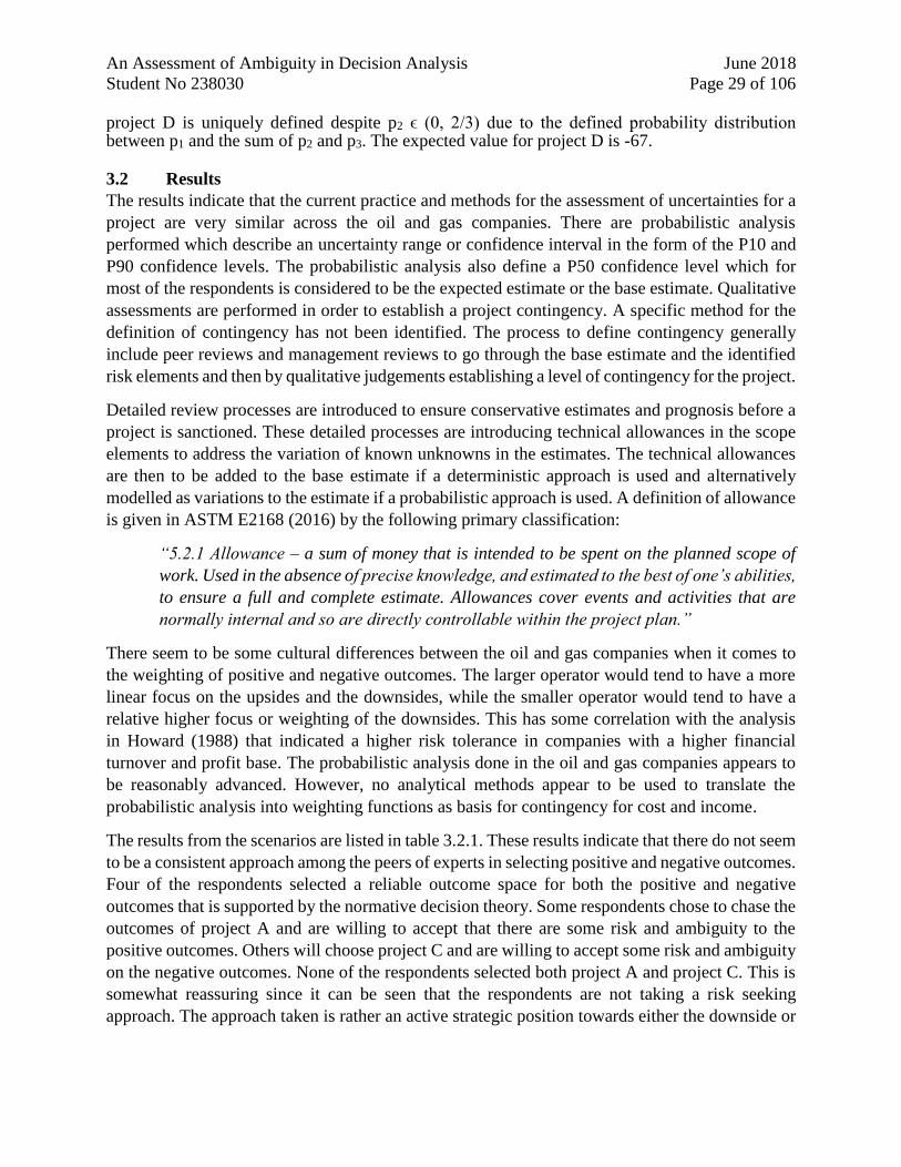
An Assessment of Ambiguity in Decision Analysis June 2018
Student No 238030 Page 29 of 106
project D is uniquely defined despite p2 ϵ (0, 2/3) due to the defined probability distribution between p1 and the sum of p2 and p3. The expected value for project D is -67.
3.2 Results
The results indicate that the current practice and methods for the assessment of uncertainties for a
project are very similar across the oil and gas companies. There are probabilistic analysis
performed which describe an uncertainty range or confidence interval in the form of the P10 and
P90 confidence levels. The probabilistic analysis also define a P50 confidence level which for
most of the respondents is considered to be the expected estimate or the base estimate. Qualitative
assessments are performed in order to establish a project contingency. A specific method for the
definition of contingency has not been identified. The process to define contingency generally
include peer reviews and management reviews to go through the base estimate and the identified
risk elements and then by qualitative judgements establishing a level of contingency for the project.
Detailed review processes are introduced to ensure conservative estimates and prognosis before a
project is sanctioned. These detailed processes are introducing technical allowances in the scope
elements to address the variation of known unknowns in the estimates. The technical allowances
are then to be added to the base estimate if a deterministic approach is used and alternatively
modelled as variations to the estimate if a probabilistic approach is used. A definition of allowance
is given in ASTM E2168 (2016) by the following primary classification:
“5.2.1 Allowance – a sum of money that is intended to be spent on the planned scope of
work. Used in the absence of precise knowledge, and estimated to the best of one’s abilities,
to ensure a full and complete estimate. Allowances cover events and activities that are
normally internal and so are directly controllable within the project plan.”
There seem to be some cultural differences between the oil and gas companies when it comes to
the weighting of positive and negative outcomes. The larger operator would tend to have a more
linear focus on the upsides and the downsides, while the smaller operator would tend to have a
relative higher focus or weighting of the downsides. This has some correlation with the analysis
in Howard (1988) that indicated a higher risk tolerance in companies with a higher financial
turnover and profit base. The probabilistic analysis done in the oil and gas companies appears to
be reasonably advanced. However, no analytical methods appear to be used to translate the
probabilistic analysis into weighting functions as basis for contingency for cost and income.
The results from the scenarios are listed in table 3.2.1. These results indicate that there do not seem
to be a consistent approach among the peers of experts in selecting positive and negative outcomes.
Four of the respondents selected a reliable outcome space for both the positive and negative
outcomes that is supported by the normative decision theory. Some respondents chose to chase the
outcomes of project A and are willing to accept that there are some risk and ambiguity to the
positive outcomes. Others will choose project C and are willing to accept some risk and ambiguity
on the negative outcomes. None of the respondents selected both project A and project C. This is
somewhat reassuring since it can be seen that the respondents are not taking a risk seeking
approach. The approach taken is rather an active strategic position towards either the downside or
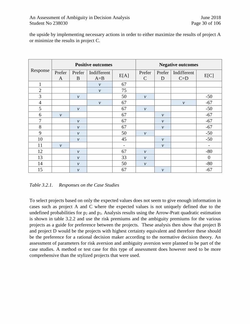
An Assessment of Ambiguity in Decision Analysis June 2018
Student No 238030 Page 30 of 106
the upside by implementing necessary actions in order to either maximize the results of project A
or minimize the results in project C.
Response
Positive outcomes Negative outcomes
Prefer
A
Prefer
B
Indifferent
A=B E[A]
Prefer
C
Prefer
D
Indifferent
C=D E[C]
1 v 67
2 v 75
3 v 50 v -50
4 v 67 v -67
5 v 67 v -50
6 v 67 v -67
7 v 67 v -67
8 v 67 v -67
9 v 50 v -50
10 v 45 v -50
11 v - v -
12 v 67 v -80
13 v 33 v 0
14 v 50 v -80
15 v 67 v -67
Table 3.2.1. Responses on the Case Studies
To select projects based on only the expected values does not seem to give enough information in
cases such as project A and C where the expected values is not uniquely defined due to the
undefined probabilities for p2 and p3. Analysis results using the Arrow-Pratt quadratic estimation
is shown in table 3.2.2 and use the risk premiums and the ambiguity premiums for the various
projects as a guide for preference between the projects. These analysis then show that project B
and project D would be the projects with highest certainty equivalent and therefore these should
be the preference for a rational decision maker according to the normative decision theory. An
assessment of parameters for risk aversion and ambiguity aversion were planned to be part of the
case studies. A method or test case for this type of assessment does however need to be more
comprehensive than the stylized projects that were used.
An Assessment of Ambiguity in Decision Analysis June 2018
Student No 238030 Page 31 of 106
Project Predicted Value Risk
premium
Ambiguity
premium
Certainty
equivalent (CE)
A 66.67 11.11 16.67
38.89
B 66.67 11.11 0.00 55.56
C -66.67 11.11 16.67 -94.44
D -66.67 11.11 0.00 -77.78
Table 3.2.2. Certainty Equivalent for the Case Studies
The project contingency can have elements of both aleatory and epistemic uncertainty. It is normal
to have a high contingency at the early phase of a project, which then is reduced as the project
definition is more matured and the epistemic uncertainty then reduced. This staged development
of contingency is defined by the project stages DG1, DG2 and DG3 which is commonly used in
the industry. There may however be large uncertainties also at project sanction (after DG3). This
may be aleatory uncertainties related to weather sensitive activities such as offshore hook-up work,
marine operations or epistemic uncertainties related to project performance of new contractors or
the use of novel technology and solutions. A definition of contingency is given in ASTM E2168
(2016) by the following primary classification:
“5.2.2 Contingency – A sum of money that is provided to cover the occurrence of
unintended departures from the planned scope of work. Used in the absence of precise
knowledge, and estimated to the best of one’s knowledge to ensure that a financial buffer
is available within a budget. Contingencies assist in mitigating the effects of unplanned
events and other risks that are external to, and are not directly controllable within, a
project plan.”
The contingency of the cost estimate seem to be based on deterministic based guidelines that may
range from 40% for DG1 to 15% for DG3. The research results indicate that there is a mixture of
probabilistic and deterministic approaches used. The P10, P50 and P90 confidence levels are
probabilistic based while the contingency is deterministic based. The research results also indicate
some inconsistency in how contingency is introduced. The contingency is either added to the P50
confidence level or included in the values of P10, P50 and P90 confidence levels.
The results confirm that there are large uncertainties in the prediction of the oil and gas production
of a field development. These uncertainties could for example be related to subsurface issues in
the form of optimistic reservoir characteristics or facility issues in the form of insufficient
processing capacity or low production efficiency. Risk and ambiguity aversion and corresponding
An Assessment of Ambiguity in Decision Analysis June 2018
Student No 238030 Page 32 of 106
premiums do however not seem to be used in the value proposition for the overall net present value
for a life of field estimate. The large uncertainties and the large consequences for a company in
the event of large negative outcome would however warrant the use of risk and ambiguity
premiums or contingencies. It should therefore be further assessed if risk and ambiguity premiums
should be introduced to account for uncertainties related to the oil and gas production.
Uncertainties in the income of the oil and gas production will also be affected by the external
factors in the form of a volatile oil price that would warrant the use of ambiguity premiums or
management reserves. A definition of reserve is given in ASTM E2168 (2016) by the following
primary classification:
“5.2.3 Reserve – A sum, usually held by management (client) to be disbursed only when
project requirements are changed. Used to provide insurance against a project or
program failing to complete on budget of for the revision of a budget in the case of
changed management or program direction and requirement.”
The results confirm that there are situations where potential large negative outcomes can result in
a decision to stop an activity or to turn down or delay a project development. These types of
decision problems with high consequence are also normally associated with ambiguity that need
to be mitigated by pre-cautionary or cautionary measures before the continuation of an activity or
a project.
3.2.1 The use of expected values and confidence intervals
The expected value or mean value represents the weighted average or the center of gravity of a
probability distribution of the outcomes. The mean value is also referred to as the P50 confidence
level although these may differ if the probability distribution is skewed. The P50 confidence level
gives equal probability of underrun and overrun and the area under the probability curve is thus
the same on both sides of the P50 value.
The questions included in the in-depth interviews were as follows:
Are you familiar with the concepts of expected value or P50 confidence level?
Do you know where the concepts of expected value or P50 confidence level are used in the
decision process?
All responses from the oil and gas companies confirmed familiarization with the use of a P50
confidence level and also confirmed that the term expected value is less frequently used. The
respondents further described that the P50 confidence level is normally used to determine a base
estimate within cost and plan for a project. One of the respondents that is managing partner-
operated assets used the P70 confidence level as the base estimate which then was considered to
be close to the P50 confidence level added with the contingency reported by the asset operator.
One respondent however referred to contingency as the difference between the base estimate and
the P50 estimate. This shows that there are some differences in the interpretation and the build- up
of the project cost estimates between the oil companies.
An Assessment of Ambiguity in Decision Analysis June 2018
Student No 238030 Page 33 of 106
A respondent that has a role as portfolio manager for capital projects described that the term
expected values is often misused. There can be occasions where managers refer to expected values
with no underlying probabilistic basis or where the expected value is a mixture of probabilistic and
deterministic approaches.
A respondent that is managing field developments described the assessments he performs before
a project sanction. He then performs a detailed process where all potential downsides and upsides
are challenged and conservative estimates and prognosis are included in order to take ownership
and maximise the probability of success in the execution of the project.
Several respondents described that there can be large uncertainties and corresponding widespread
confidence intervals in the subsurface results and advanced probabilistic analysis of uncertainties
are therefore performed within this area.
The responses describe that the uncertainty represented by the P10 and P90 confidence levels is
subject to detailed assessments of the elements that give the highest contribution to the confidence
interval variation. Sensitivity analysis with more refined or skewed probability distributions may
then be included in the detailed assessments in order to reduce the variation and give a better
description of the relevant phenomena.
3.2.2 Are there any weighting of consequences?
A decision maker is neutral to loss or gain if a negative or positive outcome is given the same
weighting. This also means that the decision maker has a linear relationship between potential
negative and potential positive outcomes.
The questions included in the in-depth interviews were as follows:
In a decision process, do you differentiate between a potential positive and a potential negative
outcome?
Do you know how this differentiation of outcomes can be done?
Are you familiar with the term of being risk neutral?
Do you agree that decisions based on expected values are a risk neutral approach?
The respondents that are managing projects describe that the weighting of potential upsides and
downsides is based on a balanced judgement of the inputs from the members of the project team.
A well performing project team will have members with different attitudes and judgements, some
may have an optimistic attitude that pushes potential upsides and some may have a more skeptical
attitude which can be used to address and find potential downsides. A mixture of these types of
personalities are required in a project team in order to ensure a balanced view and steering of the
outcomes from a project.
All responses confirmed that there is a high focus on how to reduce or mitigate the downsides or
negative outcomes. One of the respondents from a larger operator considered however that there
is a linear weighting relationship and high focus on both the negative and positive outcomes. Only
one of the respondents was aware and familiar with analytical methods for a non-linear weighting
of negative and positive outcomes. This respondent has previous experience as decision analyst.
An Assessment of Ambiguity in Decision Analysis June 2018
Student No 238030 Page 34 of 106
Most of the other respondents described the introduction of skewed probability distributions,
technical reviews, management reviews and cautionary measures to reduce or mitigate the
potential negative outcomes.
3.2.3 Familiarity with risk and ambiguity premium and certainty equivalent
Tolerance of risk or aversion to risk is a subjective judgement and expresses the decision maker’s
aversion to losses or a potential negative outcome. The potential outcomes are then based on
uncertainty assessments of the known unknowns of estimated quantities, rates and norms of the
technical solution or scope. Ambiguity is a term used to describe uncertainty when you are not
confident in assigning a probability distribution. This could refer to uncertainty of unspecified or
unknown elements of a technical solution or scope. But it could also include externalities that lie
outside of the project’s control. When faced with risk and ambiguity the decision maker may
therefore be willing to pay a premium in order to mitigate or neutralize his uncertainty exposure.
The certainty equivalent for a project subject to risk and ambiguity is then the difference between
a predicted expected value and the risk and ambiguity premiums.
The questions included in the in-depth interviews were as follows:
Do you know how a decision maker’s risk aversion or contingency is implemented in the
decision process?
Do you know how a decision maker’s ambiguity aversion or budget reserve is implemented
in the decision process?
Are you familiar with the term certainty equivalent value and the use of contingency and
budget reserves in a decision process?
Only one respondent confirmed that he was familiar with the terminology and use of risk premium,
ambiguity premium and certainty equivalent. This respondent was the one with experience as
decision analyst. All responses confirmed that contingency and reserves are commonly used in
project cost definition. The contingency would then include elements of both risk and ambiguity
for the defined technical solution and scope. The respondents describe that the project cost
definition are normally well defined by detailed base cost estimates that is matured during the
project stages leading up to the decision gate for project sanction and these are also updated at
different stages during the project execution. The respondents describe the process of defining the
contingency and reserve as a qualitative process where the 80% confidence interval and the
corresponding elements with uncertainty are subject to detailed reviews by technical peers group
and finally decided in management reviews. Contingency ranging from 5% to 20% of the base
estimate is used at project sanction. Examples referred to by one of the respondents were related
to the contingency cost of jacket fabrication and jacket installation. Jacket fabrication performed
in a new fabrication yards are given a higher contingency contribution than the familiar fabrication
yards with a strong track record of previous jacket fabrication deliveries to company. For the jacket
installation, the company has experience with launched jackets and no or limited experience with
lifted jackets. According to the respondent, the lifted jacket concept is therefore given a
contingency contribution of 20% and the launched jacket is given a contingency contribution of
12%.
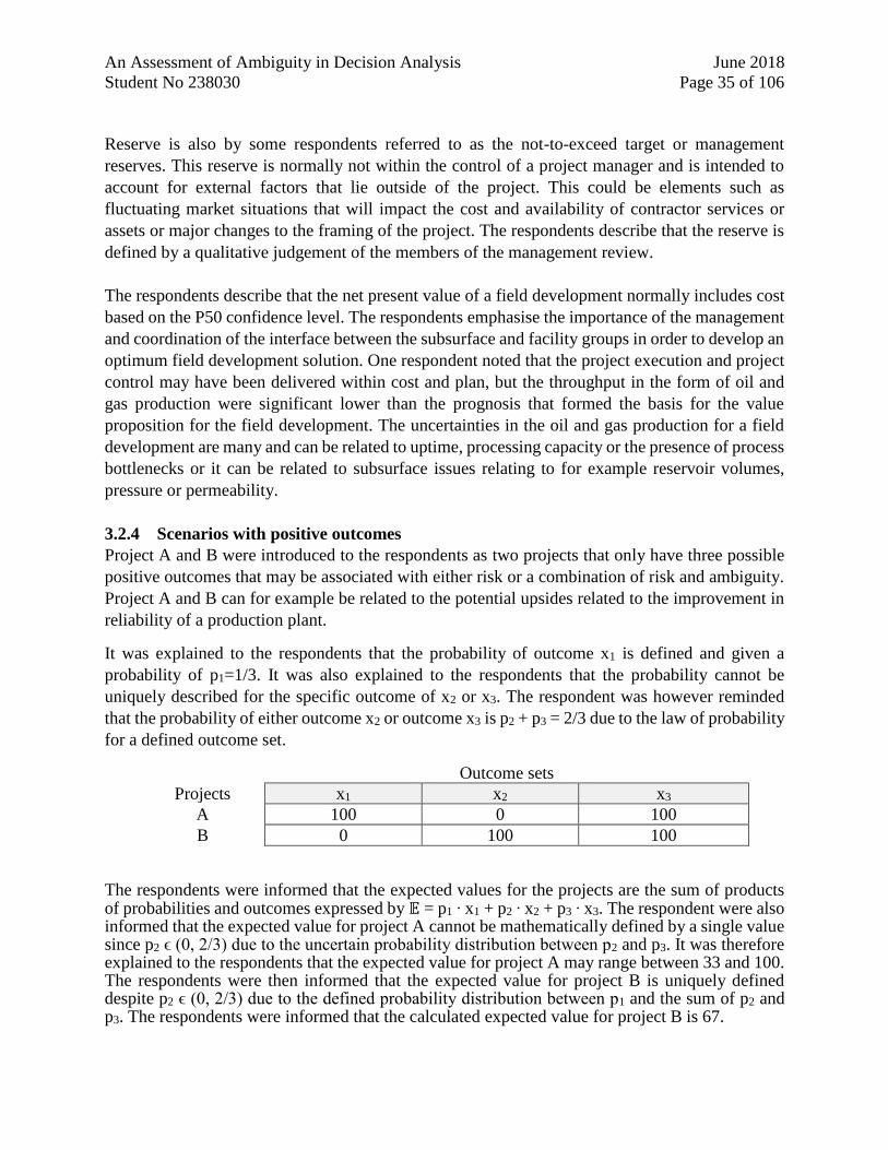
An Assessment of Ambiguity in Decision Analysis June 2018
Student No 238030 Page 35 of 106
Reserve is also by some respondents referred to as the not-to-exceed target or management
reserves. This reserve is normally not within the control of a project manager and is intended to
account for external factors that lie outside of the project. This could be elements such as
fluctuating market situations that will impact the cost and availability of contractor services or
assets or major changes to the framing of the project. The respondents describe that the reserve is
defined by a qualitative judgement of the members of the management review.
The respondents describe that the net present value of a field development normally includes cost
based on the P50 confidence level. The respondents emphasise the importance of the management
and coordination of the interface between the subsurface and facility groups in order to develop an
optimum field development solution. One respondent noted that the project execution and project
control may have been delivered within cost and plan, but the throughput in the form of oil and
gas production were significant lower than the prognosis that formed the basis for the value
proposition for the field development. The uncertainties in the oil and gas production for a field
development are many and can be related to uptime, processing capacity or the presence of process
bottlenecks or it can be related to subsurface issues relating to for example reservoir volumes,
pressure or permeability.
3.2.4 Scenarios with positive outcomes
Project A and B were introduced to the respondents as two projects that only have three possible
positive outcomes that may be associated with either risk or a combination of risk and ambiguity.
Project A and B can for example be related to the potential upsides related to the improvement in
reliability of a production plant.
It was explained to the respondents that the probability of outcome x1 is defined and given a
probability of p1=1/3. It was also explained to the respondents that the probability cannot be
uniquely described for the specific outcome of x2 or x3. The respondent was however reminded
that the probability of either outcome x2 or outcome x3 is p2 + p3 = 2/3 due to the law of probability
for a defined outcome set.
Outcome sets
Projects x1 x2 x3
A 100 0 100
B 0 100 100
The respondents were informed that the expected values for the projects are the sum of products of probabilities and outcomes expressed by 𝔼 = p1 ∙ x1 + p2 ∙ x2 + p3 ∙ x3. The respondent were also informed that the expected value for project A cannot be mathematically defined by a single value since p2 ϵ (0, 2/3) due to the uncertain probability distribution between p2 and p3. It was therefore explained to the respondents that the expected value for project A may range between 33 and 100. The respondents were then informed that the expected value for project B is uniquely defined despite p2 ϵ (0, 2/3) due to the defined probability distribution between p1 and the sum of p2 and p3. The respondents were informed that the calculated expected value for project B is 67.
An Assessment of Ambiguity in Decision Analysis June 2018
Student No 238030 Page 36 of 106
The questions included in the in-depth interviews were as follows:
Please have a look at project A and project B, would you prefer one out of these two projects
or do you consider them to be indifferent?
Can you explain how you arrived at your choice between project A and project B?
What would you consider as an appropriate expected value for project A?
If you had more information about P10 and P90 for the projects would you then assign a reserve
or buffer to the expected values to account for the statistical variation in project B?
Would you assign a reserve or buffer to the expected values to account for the unknown
unknowns in project A?
Can you recall a similar decision setting as for project A where you are not able to describe the
probabilities for a specific outcome?
Eight of the responses were a preference for project B which would indicate a preference for a
reliable or predictable opportunity space. Three of the responses were indifferent between the
projects A and B. The reason for this indifference was explained by a prediction of equal
probabilities for all outcomes. Two of the responses were a preference for project A as the
opportunity for maximizing the positive results was considered highest for project A. The
responses on the expected value prediction for project A resulted in a mean value of 62.6 and a
standard deviation of 9.6.
All responses confirmed that a margin for risk and ambiguity would be introduced. More
background information on the decision setting and basis for the numbers presented for the projects
is however required in order to assess the appropriate level of the required risk and ambiguity
margin. Several of the respondents confirmed that projects with elements of variable or undefined
probabilities are common. There can be many subprojects that have probabilities of variable
degrees of precision that the project manager has to understand and have a feel or intuition on what
to challenge and monitor.
3.2.5 Scenarios with negative outcomes
Project C and D were introduced to the respondents as two projects that only have three possible
negative outcomes that may be associated with either risk or a combination of risk and ambiguity.
Project C and D were explained to the respondents as an example related to potential cost increases
for a contracted delivery. The respondents were informed that the probability of outcome x1 is
defined and given a probability of p1=1/3. The respondents were informed that the probability is
not defined for the specific outcome of x2 or x3. It was explained to the respondents that the
probability of either outcome x2 or outcome x3 is p2 + p3 = 2/3 due to the law of probability for a
defined outcome set.
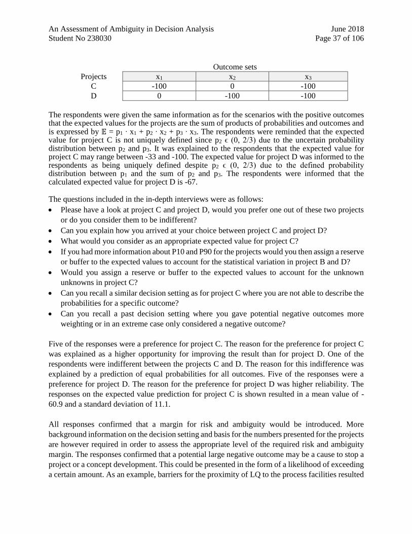
An Assessment of Ambiguity in Decision Analysis June 2018
Student No 238030 Page 37 of 106
Outcome sets
Projects x1 x2 x3
C -100 0 -100
D 0 -100 -100
The respondents were given the same information as for the scenarios with the positive outcomes that the expected values for the projects are the sum of products of probabilities and outcomes and is expressed by 𝔼 = p1 ∙ x1 + p2 ∙ x2 + p3 ∙ x3. The respondents were reminded that the expected value for project C is not uniquely defined since p2 ϵ (0, 2/3) due to the uncertain probability distribution between p2 and p3. It was explained to the respondents that the expected value for project C may range between -33 and -100. The expected value for project D was informed to the respondents as being uniquely defined despite p2 ϵ (0, 2/3) due to the defined probability distribution between p1 and the sum of p2 and p3. The respondents were informed that the calculated expected value for project D is -67.
The questions included in the in-depth interviews were as follows:
Please have a look at project C and project D, would you prefer one out of these two projects
or do you consider them to be indifferent?
Can you explain how you arrived at your choice between project C and project D?
What would you consider as an appropriate expected value for project C?
If you had more information about P10 and P90 for the projects would you then assign a reserve
or buffer to the expected values to account for the statistical variation in project B and D?
Would you assign a reserve or buffer to the expected values to account for the unknown
unknowns in project C?
Can you recall a similar decision setting as for project C where you are not able to describe the
probabilities for a specific outcome?
Can you recall a past decision setting where you gave potential negative outcomes more
weighting or in an extreme case only considered a negative outcome?
Five of the responses were a preference for project C. The reason for the preference for project C
was explained as a higher opportunity for improving the result than for project D. One of the
respondents were indifferent between the projects C and D. The reason for this indifference was
explained by a prediction of equal probabilities for all outcomes. Five of the responses were a
preference for project D. The reason for the preference for project D was higher reliability. The
responses on the expected value prediction for project C is shown resulted in a mean value of -
60.9 and a standard deviation of 11.1.
All responses confirmed that a margin for risk and ambiguity would be introduced. More
background information on the decision setting and basis for the numbers presented for the projects
are however required in order to assess the appropriate level of the required risk and ambiguity
margin. The responses confirmed that a potential large negative outcome may be a cause to stop a
project or a concept development. This could be presented in the form of a likelihood of exceeding
a certain amount. As an example, barriers for the proximity of LQ to the process facilities resulted

An Assessment of Ambiguity in Decision Analysis June 2018
Student No 238030 Page 38 of 106
in a low expected safety factor which then turned this concept down. This focus on negative
outcomes is typical when addressing safety, environment and quality issues. Within subsurface,
one of the respondents noted that the decision to proceed with a field development project largely
depends on the results from the appraisal wells. Poor results from appraisal wells can increase the
uncertainty of a reservoir that can lead to a stop or delay of a field development project.
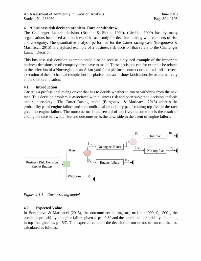
An Assessment of Ambiguity in Decision Analysis June 2018
Student No 238030 Page 39 of 106
4 A business risk decision problem- Race or withdraw
The Challenger Launch decision (Brittain & Sitkin, 1990), (Liedtka, 1990) has by many
organisations been used as a business risk case study for decision making with elements of risk
and ambiguity. The quantitative analysis performed for the Carter racing case (Borgonovo &
Marinacci, 2015) is a stylised example of a business risk decision that refers to the Challenger
Launch Decision.
This business risk decision example could also be seen as a stylised example of the important
business decisions an oil company often have to make. These decisions can for example be related
to the selection of a Norwegian or an Asian yard for a platform contract or the trade-off between
execution of the mechanical completion of a platform on an onshore fabrication site or alternatively
at the offshore location.
4.1 Introduction
Carter is a professional racing driver that has to decide whether to run or withdraw from the next
race. This decision problem is associated with business risk and been subject to decision analysis
under uncertainty. The Carter Racing model (Borgonovo & Marinacci, 2015) address the
probability p2 of engine failure and the conditional probability p1 of coming top five in the race
given no engine failure. The outcome m1 is the reward of top five, outcome m2 is the result of
ending the race below top five and outcome m3 is the downside in the event of engine failure.
Figure 4.1.1 Carter racing model
4.2 Expected Value
In Borgonovo & Marinacci (2015), the outcome set is {m1, m2, m3} = {1000, 0, -500}, the
predicted probability of engine failure given as p2 =0.30 and the conditional probability of coming
in top five given as p1=5/7. The expected value of the decision to run or not to run can then be
calculated as follows:
No engine failure
Engine failure
Top five
Not top five
p2
1-p2
p1
1-p1Run
Withdraw
m1
m2
m3
0
Business Risk Decision
Carter Racing
An Assessment of Ambiguity in Decision Analysis June 2018
Student No 238030 Page 40 of 106
HRun=(1-p2) ∙ [p1 ∙m1+(1-p1) ∙ m2]+p2 ∙ m3=(1-0.3) ∙ [5/7 ∙ (1000)+(1-5/7) ∙ (0)]+0.3 ∙ (-500)= 350
HWithdraw=0
4.3 Smooth ambiguity aversion
In Borgonovo & Marinacci (2015), the smooth ambiguity aversion model is included. This is also
referred to as the KMM functional (Klibanoff, et al., 2005). This model can be used to estimate
risk and ambiguity premiums and the corresponding certainty equivalent. A second order
probability distribution for the predicted probability is then first included in the Carter Racing
model by a combination of two sets of beta distributions where the expected probability value is
similar to predicted probability value. The expected value for the beta distribution with a=2 and
b=6 is ¼ and the expected value for the beta distribution with a=6 and b=2 is ¾. The expected
probability value for the second order probability distribution is adjusted to be similar to the
predicted probability value by a factor m as given by the formula; p2Pred = (1-m) ∙ beta(2,6) + m ∙
beta(6,2) = (1-m)∙1/4 + m∙3/4. The factor m can therefore be calculated as; m = (p2Pred – ¼) ∙ 2 =
0.10.
The calculation of the risk and ambiguity premiums is an iterative process where the risk tolerance
factor and the ambiguity aversion parameter have to be balanced by the use of the smooth
ambiguity model (KMM functional) and the Arrow-Pratt (AP) quadratic estimation method. These
methods are described in Appendix B.
The risk and ambiguity premiums are calculated by use of both the smooth ambiguity model
(KMM functional) and the extended form of the AP quadratic estimation. The extended AP
quadratic estimation also estimate the portion of risk premium and ambiguity premium. The
certainty equivalent represents the difference between the predicted mean value and the risk and
ambiguity premiums. The risk and ambiguity premium and corresponding certainty equivalent is
shown in the table below and is balanced with a risk aversion parameter of 1/1000 and an
ambiguity aversion parameter of 1/100.
KMM functional AP Quadratic Estimation
Certainty equivalent, C(Run)= -143.31 -147.52 -148.771 -162.92
Risk premium, ПAM(Run)= 495.461 497.562 226.661 226.252
Ambiguity premium, ПAM(Run)= 274.421 286.652
1) Analysis results derived from model developed in Excel
2) Analysis results given in Borgonovo & Marinacci (2015)
4.4 Risk aversion
The decision three for the Carter Racing decision problem has been modelled by use of the
Precision Tree Software. A concave exponential function with a risk tolerance factor of 1000 have
been used. The certainty equivalent that include risk aversion have then been calculated to
C(Run)= 129.5. This is close to the certainty equivalent with risk aversion of C(Run)=123.75 as
given in Borgonovo & Marinacci (2015).
An Assessment of Ambiguity in Decision Analysis June 2018
Student No 238030 Page 41 of 106
Figure 4.4.1 CE for Carter Racing with risk aversion
4.5 Extreme Risk and Ambiguity aversion
The certainty equivalent for the Wald Maximin Functional is the worst possible outcome for the
decision alternatives. The certainty equivalent values for Wald Maximin Functional is therefore
C(Run) = -500 and C(Withdraw) = 0.
4.6 Decision maker’s preferences for the Carter Racing
The objective with the analysis was to assess the whether to run or withdraw from the race.
Analysis have been performed to assess the expected values and the certainty equivalent values
for the decision alternatives. Several methods for analysis the certainty equivalent values have
been applied that addresses the preferences for a decision maker with risk aversion, risk and
ambiguity aversion and extreme risk and ambiguity aversion. The results from these analysis
methods can be summarised as follows:
• The expected value is maximised for the decision to run
• The risk and ambiguity averse certainty equivalent is maximised for the decision to
withdraw from the race
• The risk averse certainty equivalent is maximised for the decision to run
• The extreme risk and ambiguity averse certainty equivalent is maximised for the decision
to withdraw from the race
A risk neutral decision maker will have a preference to run since expected value is highest for this
alternative. A risk and ambiguity averse decision maker will have a preference to withdraw since
the certainty equivalent for the KMM functional and Arrow-Pratt Approximation is highest for
this alternative. A risk averse decision maker will have a preference to run since the certainty
equivalent calculated by use of the Precision Tree software is highest for this alternative. An
extreme risk and ambiguity decision maker will have a preference to withdraw since the maximum
worst consequence is minimised for this alternative.
71.4% 50.0%
1000 1000
70.0% CE
0 601
28.6% 20.0%
0 0
TRUE CE
0 129.5
30.0% 30.0%
-500 -500
CE
129.5
FALSE 0.0%
0 0
Carter Racing?
Withdraw
Run
Engine failure
No engine failure
Top five
Not top five
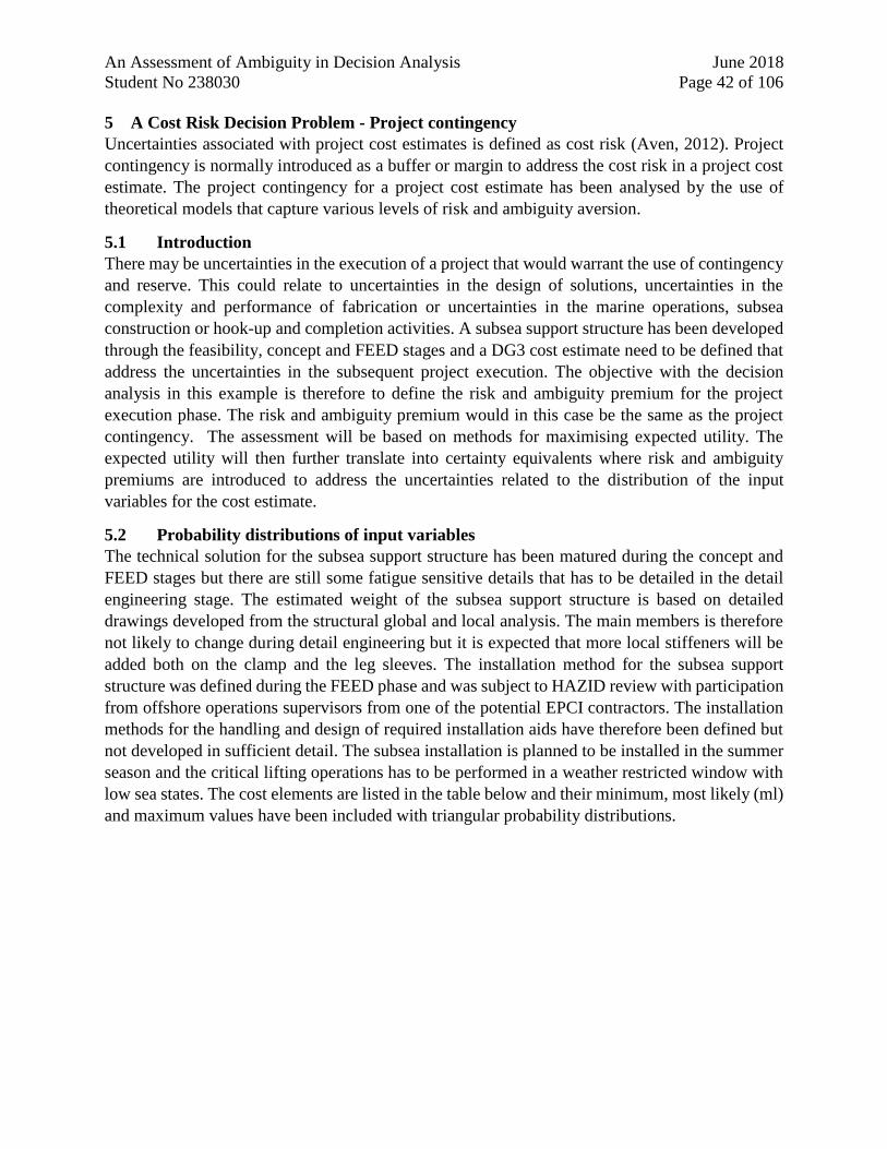
An Assessment of Ambiguity in Decision Analysis June 2018
Student No 238030 Page 42 of 106
5 A Cost Risk Decision Problem - Project contingency
Uncertainties associated with project cost estimates is defined as cost risk (Aven, 2012). Project
contingency is normally introduced as a buffer or margin to address the cost risk in a project cost
estimate. The project contingency for a project cost estimate has been analysed by the use of
theoretical models that capture various levels of risk and ambiguity aversion.
5.1 Introduction
There may be uncertainties in the execution of a project that would warrant the use of contingency
and reserve. This could relate to uncertainties in the design of solutions, uncertainties in the
complexity and performance of fabrication or uncertainties in the marine operations, subsea
construction or hook-up and completion activities. A subsea support structure has been developed
through the feasibility, concept and FEED stages and a DG3 cost estimate need to be defined that
address the uncertainties in the subsequent project execution. The objective with the decision
analysis in this example is therefore to define the risk and ambiguity premium for the project
execution phase. The risk and ambiguity premium would in this case be the same as the project
contingency. The assessment will be based on methods for maximising expected utility. The
expected utility will then further translate into certainty equivalents where risk and ambiguity
premiums are introduced to address the uncertainties related to the distribution of the input
variables for the cost estimate.
5.2 Probability distributions of input variables
The technical solution for the subsea support structure has been matured during the concept and
FEED stages but there are still some fatigue sensitive details that has to be detailed in the detail
engineering stage. The estimated weight of the subsea support structure is based on detailed
drawings developed from the structural global and local analysis. The main members is therefore
not likely to change during detail engineering but it is expected that more local stiffeners will be
added both on the clamp and the leg sleeves. The installation method for the subsea support
structure was defined during the FEED phase and was subject to HAZID review with participation
from offshore operations supervisors from one of the potential EPCI contractors. The installation
methods for the handling and design of required installation aids have therefore been defined but
not developed in sufficient detail. The subsea installation is planned to be installed in the summer
season and the critical lifting operations has to be performed in a weather restricted window with
low sea states. The cost elements are listed in the table below and their minimum, most likely (ml)
and maximum values have been included with triangular probability distributions.
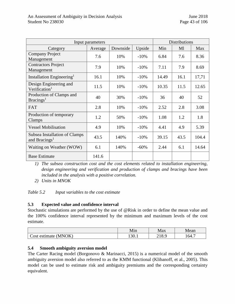
An Assessment of Ambiguity in Decision Analysis June 2018
Student No 238030 Page 43 of 106
Input parameters Distributions
Category Average Downside Upside Min Ml Max
Company Project
Management 7.6 10% -10% 6.84 7.6 8.36
Contractors Project
Management 7.9 10% -10% 7.11 7.9 8.69
Installation Engineering1 16.1 10% -10% 14.49 16.1 17,71
Design Engineering and
Verification1 11.5 10% -10% 10.35 11.5 12.65
Production of Clamps and
Bracings1 40 30% -10% 36 40 52
FAT 2.8 10% -10% 2.52 2.8 3.08
Production of temporary
Clamps 1.2 50% -10% 1.08 1.2 1.8
Vessel Mobilisation 4.9 10% -10% 4.41 4.9 5.39
Subsea Installation of Clamps
and Bracings1 43.5 140% -10% 39.15 43.5 104.4
Waiting on Weather (WOW) 6.1 140% -60% 2.44 6.1 14.64
Base Estimate 141.6
1) The subsea construction cost and the cost elements related to installation engineering,
design engineering and verification and production of clamps and bracings have been
included in the analysis with a positive correlation.
2) Units in MNOK
Table 5.2 Input variables to the cost estimate
5.3 Expected value and confidence interval
Stochastic simulations are performed by the use of @Risk in order to define the mean value and
the 100% confidence interval represented by the minimum and maximum levels of the cost
estimate.
Min Max Mean
Cost estimate (MNOK) 130.1 218.9 164.7
5.4 Smooth ambiguity aversion model
The Carter Racing model (Borgonovo & Marinacci, 2015) is a numerical model of the smooth
ambiguity aversion model also referred to as the KMM functional (Klibanoff, et al., 2005). This
model can be used to estimate risk and ambiguity premiums and the corresponding certainty
equivalent.
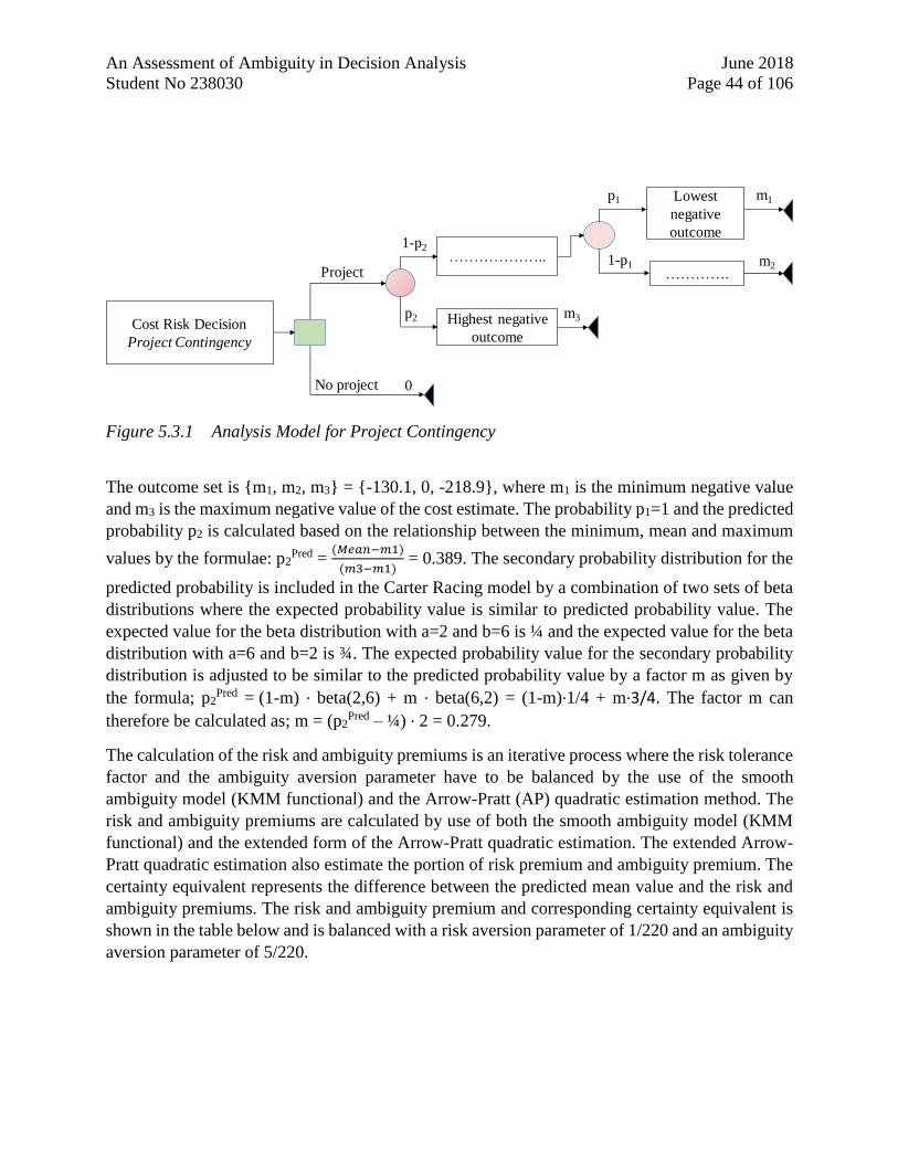
An Assessment of Ambiguity in Decision Analysis June 2018
Student No 238030 Page 44 of 106
Figure 5.3.1 Analysis Model for Project Contingency
The outcome set is {m1, m2, m3} = {-130.1, 0, -218.9}, where m1 is the minimum negative value
and m3 is the maximum negative value of the cost estimate. The probability p1=1 and the predicted
probability p2 is calculated based on the relationship between the minimum, mean and maximum
values by the formulae: p2Pred =
(𝑀𝑒𝑎𝑛−𝑚1)
(𝑚3−𝑚1) = 0.389. The secondary probability distribution for the
predicted probability is included in the Carter Racing model by a combination of two sets of beta
distributions where the expected probability value is similar to predicted probability value. The
expected value for the beta distribution with a=2 and b=6 is ¼ and the expected value for the beta
distribution with a=6 and b=2 is ¾. The expected probability value for the secondary probability
distribution is adjusted to be similar to the predicted probability value by a factor m as given by
the formula; p2Pred = (1-m) ∙ beta(2,6) + m ∙ beta(6,2) = (1-m)∙1/4 + m∙3/4. The factor m can
therefore be calculated as; m = (p2Pred – ¼) ∙ 2 = 0.279.
The calculation of the risk and ambiguity premiums is an iterative process where the risk tolerance
factor and the ambiguity aversion parameter have to be balanced by the use of the smooth
ambiguity model (KMM functional) and the Arrow-Pratt (AP) quadratic estimation method. The
risk and ambiguity premiums are calculated by use of both the smooth ambiguity model (KMM
functional) and the extended form of the Arrow-Pratt quadratic estimation. The extended Arrow-
Pratt quadratic estimation also estimate the portion of risk premium and ambiguity premium. The
certainty equivalent represents the difference between the predicted mean value and the risk and
ambiguity premiums. The risk and ambiguity premium and corresponding certainty equivalent is
shown in the table below and is balanced with a risk aversion parameter of 1/220 and an ambiguity
aversion parameter of 5/220.
………………..
Highest negative
outcome
Lowest
negative
outcome
………….
p2
1-p2
p1
1-p1Project
No project
m1
m2
m3
0
Cost Risk Decision
Project Contingency
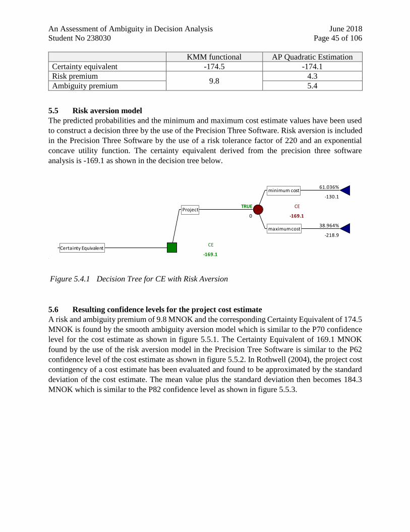
An Assessment of Ambiguity in Decision Analysis June 2018
Student No 238030 Page 45 of 106
KMM functional AP Quadratic Estimation
Certainty equivalent -174.5 -174.1
Risk premium 9.8
4.3
Ambiguity premium 5.4
5.5 Risk aversion model
The predicted probabilities and the minimum and maximum cost estimate values have been used
to construct a decision three by the use of the Precision Three Software. Risk aversion is included
in the Precision Three Software by the use of a risk tolerance factor of 220 and an exponential
concave utility function. The certainty equivalent derived from the precision three software
analysis is -169.1 as shown in the decision tree below.
Figure 5.4.1 Decision Tree for CE with Risk Aversion
5.6 Resulting confidence levels for the project cost estimate
A risk and ambiguity premium of 9.8 MNOK and the corresponding Certainty Equivalent of 174.5
MNOK is found by the smooth ambiguity aversion model which is similar to the P70 confidence
level for the cost estimate as shown in figure 5.5.1. The Certainty Equivalent of 169.1 MNOK
found by the use of the risk aversion model in the Precision Tree Software is similar to the P62
confidence level of the cost estimate as shown in figure 5.5.2. In Rothwell (2004), the project cost
contingency of a cost estimate has been evaluated and found to be approximated by the standard
deviation of the cost estimate. The mean value plus the standard deviation then becomes 184.3
MNOK which is similar to the P82 confidence level as shown in figure 5.5.3.
61.036% 61.036%
-130.1 -130.1
TRUE CE
0 -169.1
38.964% 38.964%
-218.9 -218.9
CE
-169.1Certainty Equivalent
Project
minimum cost
maximum cost
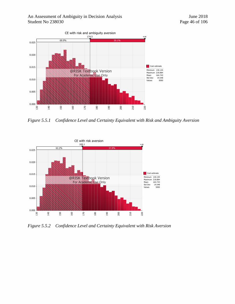
An Assessment of Ambiguity in Decision Analysis June 2018
Student No 238030 Page 46 of 106
Figure 5.5.1 Confidence Level and Certainty Equivalent with Risk and Ambiguity Aversion
Figure 5.5.2 Confidence Level and Certainty Equivalent with Risk Aversion
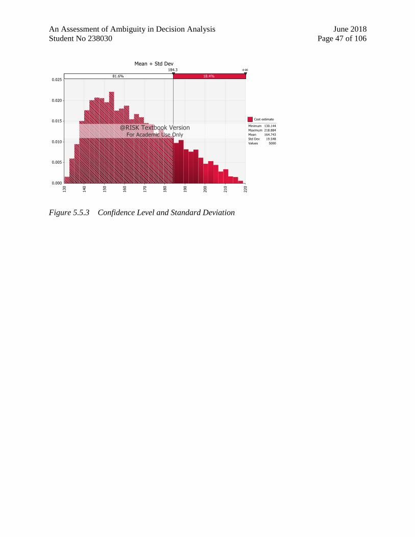
An Assessment of Ambiguity in Decision Analysis June 2018
Student No 238030 Page 47 of 106
Figure 5.5.3 Confidence Level and Standard Deviation
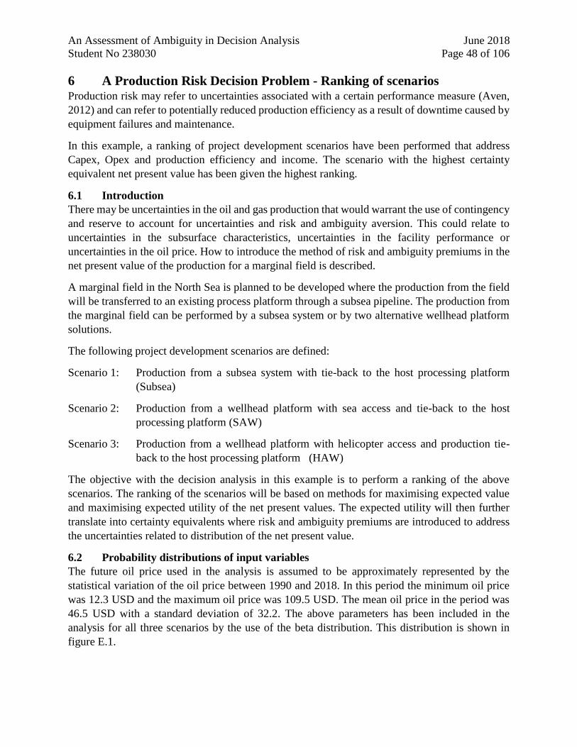
An Assessment of Ambiguity in Decision Analysis June 2018
Student No 238030 Page 48 of 106
6 A Production Risk Decision Problem - Ranking of scenarios Production risk may refer to uncertainties associated with a certain performance measure (Aven,
2012) and can refer to potentially reduced production efficiency as a result of downtime caused by
equipment failures and maintenance.
In this example, a ranking of project development scenarios have been performed that address
Capex, Opex and production efficiency and income. The scenario with the highest certainty
equivalent net present value has been given the highest ranking.
6.1 Introduction
There may be uncertainties in the oil and gas production that would warrant the use of contingency
and reserve to account for uncertainties and risk and ambiguity aversion. This could relate to
uncertainties in the subsurface characteristics, uncertainties in the facility performance or
uncertainties in the oil price. How to introduce the method of risk and ambiguity premiums in the
net present value of the production for a marginal field is described.
A marginal field in the North Sea is planned to be developed where the production from the field
will be transferred to an existing process platform through a subsea pipeline. The production from
the marginal field can be performed by a subsea system or by two alternative wellhead platform
solutions.
The following project development scenarios are defined:
Scenario 1: Production from a subsea system with tie-back to the host processing platform
(Subsea)
Scenario 2: Production from a wellhead platform with sea access and tie-back to the host
processing platform (SAW)
Scenario 3: Production from a wellhead platform with helicopter access and production tie-
back to the host processing platform (HAW)
The objective with the decision analysis in this example is to perform a ranking of the above
scenarios. The ranking of the scenarios will be based on methods for maximising expected value
and maximising expected utility of the net present values. The expected utility will then further
translate into certainty equivalents where risk and ambiguity premiums are introduced to address
the uncertainties related to distribution of the net present value.
6.2 Probability distributions of input variables
The future oil price used in the analysis is assumed to be approximately represented by the
statistical variation of the oil price between 1990 and 2018. In this period the minimum oil price
was 12.3 USD and the maximum oil price was 109.5 USD. The mean oil price in the period was
46.5 USD with a standard deviation of 32.2. The above parameters has been included in the
analysis for all three scenarios by the use of the beta distribution. This distribution is shown in
figure E.1.
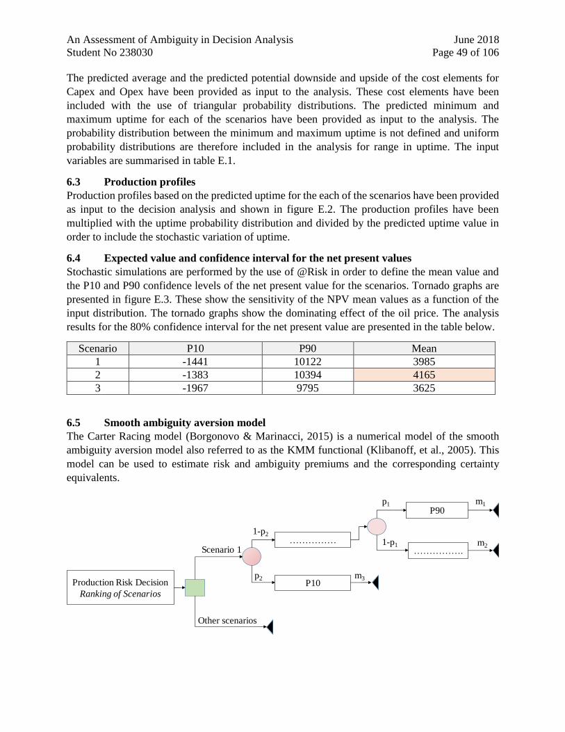
An Assessment of Ambiguity in Decision Analysis June 2018
Student No 238030 Page 49 of 106
The predicted average and the predicted potential downside and upside of the cost elements for
Capex and Opex have been provided as input to the analysis. These cost elements have been
included with the use of triangular probability distributions. The predicted minimum and
maximum uptime for each of the scenarios have been provided as input to the analysis. The
probability distribution between the minimum and maximum uptime is not defined and uniform
probability distributions are therefore included in the analysis for range in uptime. The input
variables are summarised in table E.1.
6.3 Production profiles
Production profiles based on the predicted uptime for the each of the scenarios have been provided
as input to the decision analysis and shown in figure E.2. The production profiles have been
multiplied with the uptime probability distribution and divided by the predicted uptime value in
order to include the stochastic variation of uptime.
6.4 Expected value and confidence interval for the net present values
Stochastic simulations are performed by the use of @Risk in order to define the mean value and
the P10 and P90 confidence levels of the net present value for the scenarios. Tornado graphs are
presented in figure E.3. These show the sensitivity of the NPV mean values as a function of the
input distribution. The tornado graphs show the dominating effect of the oil price. The analysis
results for the 80% confidence interval for the net present value are presented in the table below.
Scenario P10 P90 Mean
1 -1441 10122 3985
2 -1383 10394 4165
3 -1967 9795 3625
6.5 Smooth ambiguity aversion model
The Carter Racing model (Borgonovo & Marinacci, 2015) is a numerical model of the smooth
ambiguity aversion model also referred to as the KMM functional (Klibanoff, et al., 2005). This
model can be used to estimate risk and ambiguity premiums and the corresponding certainty
equivalents.
……………
P10
P90
…………….
p2
1-p2
p1
1-p1Scenario 1
Other scenarios
m1
m2
m3Production Risk Decision
Ranking of Scenarios
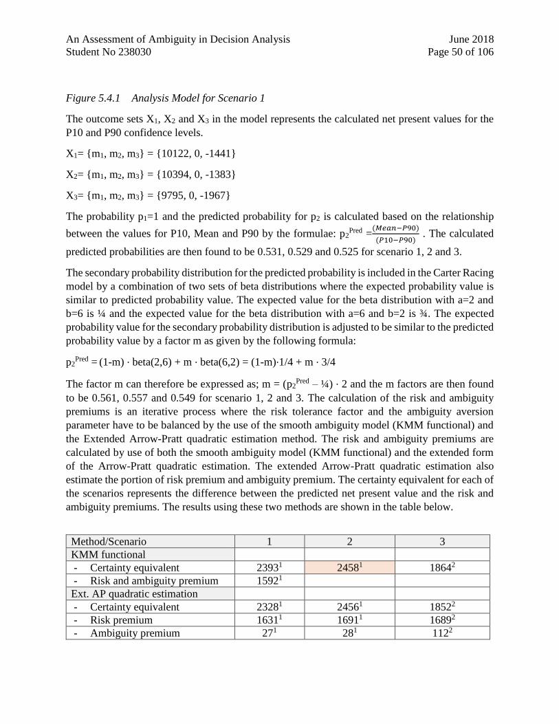
An Assessment of Ambiguity in Decision Analysis June 2018
Student No 238030 Page 50 of 106
Figure 5.4.1 Analysis Model for Scenario 1
The outcome sets X1, X2 and X3 in the model represents the calculated net present values for the
P10 and P90 confidence levels.
X1= {m1, m2, m3} = {10122, 0, -1441}
X2= {m1, m2, m3} = {10394, 0, -1383}
X3= {m1, m2, m3} = {9795, 0, -1967}
The probability p1=1 and the predicted probability for p2 is calculated based on the relationship
between the values for P10, Mean and P90 by the formulae: p2Pred =
(𝑀𝑒𝑎𝑛−𝑃90)
(𝑃10−𝑃90) . The calculated
predicted probabilities are then found to be 0.531, 0.529 and 0.525 for scenario 1, 2 and 3.
The secondary probability distribution for the predicted probability is included in the Carter Racing
model by a combination of two sets of beta distributions where the expected probability value is
similar to predicted probability value. The expected value for the beta distribution with a=2 and
b=6 is ¼ and the expected value for the beta distribution with a=6 and b=2 is ¾. The expected
probability value for the secondary probability distribution is adjusted to be similar to the predicted
probability value by a factor m as given by the following formula:
p2Pred = (1-m) ∙ beta(2,6) + m ∙ beta(6,2) = (1-m)∙1/4 + m ∙ 3/4
The factor m can therefore be expressed as; m = (p2Pred – ¼) ∙ 2 and the m factors are then found
to be 0.561, 0.557 and 0.549 for scenario 1, 2 and 3. The calculation of the risk and ambiguity
premiums is an iterative process where the risk tolerance factor and the ambiguity aversion
parameter have to be balanced by the use of the smooth ambiguity model (KMM functional) and
the Extended Arrow-Pratt quadratic estimation method. The risk and ambiguity premiums are
calculated by use of both the smooth ambiguity model (KMM functional) and the extended form
of the Arrow-Pratt quadratic estimation. The extended Arrow-Pratt quadratic estimation also
estimate the portion of risk premium and ambiguity premium. The certainty equivalent for each of
the scenarios represents the difference between the predicted net present value and the risk and
ambiguity premiums. The results using these two methods are shown in the table below.
Method/Scenario 1 2 3
KMM functional
- Certainty equivalent 23931 24581 18642
- Risk and ambiguity premium 15921
Ext. AP quadratic estimation
- Certainty equivalent 23281 24561 18522
- Risk premium 16311 16911 16892
- Ambiguity premium 271 281 1122
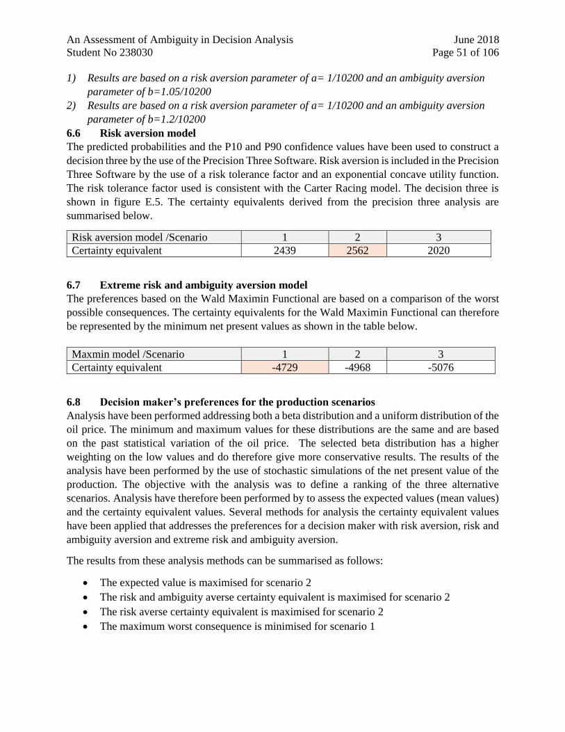
An Assessment of Ambiguity in Decision Analysis June 2018
Student No 238030 Page 51 of 106
1) Results are based on a risk aversion parameter of a= 1/10200 and an ambiguity aversion
parameter of b=1.05/10200
2) Results are based on a risk aversion parameter of a= 1/10200 and an ambiguity aversion
parameter of b=1.2/10200
6.6 Risk aversion model
The predicted probabilities and the P10 and P90 confidence values have been used to construct a
decision three by the use of the Precision Three Software. Risk aversion is included in the Precision
Three Software by the use of a risk tolerance factor and an exponential concave utility function.
The risk tolerance factor used is consistent with the Carter Racing model. The decision three is
shown in figure E.5. The certainty equivalents derived from the precision three analysis are
summarised below.
Risk aversion model /Scenario 1 2 3
Certainty equivalent 2439 2562 2020
6.7 Extreme risk and ambiguity aversion model
The preferences based on the Wald Maximin Functional are based on a comparison of the worst
possible consequences. The certainty equivalents for the Wald Maximin Functional can therefore
be represented by the minimum net present values as shown in the table below.
Maxmin model /Scenario 1 2 3
Certainty equivalent -4729 -4968 -5076
6.8 Decision maker’s preferences for the production scenarios
Analysis have been performed addressing both a beta distribution and a uniform distribution of the
oil price. The minimum and maximum values for these distributions are the same and are based
on the past statistical variation of the oil price. The selected beta distribution has a higher
weighting on the low values and do therefore give more conservative results. The results of the
analysis have been performed by the use of stochastic simulations of the net present value of the
production. The objective with the analysis was to define a ranking of the three alternative
scenarios. Analysis have therefore been performed by to assess the expected values (mean values)
and the certainty equivalent values. Several methods for analysis the certainty equivalent values
have been applied that addresses the preferences for a decision maker with risk aversion, risk and
ambiguity aversion and extreme risk and ambiguity aversion.
The results from these analysis methods can be summarised as follows:
The expected value is maximised for scenario 2
The risk and ambiguity averse certainty equivalent is maximised for scenario 2
The risk averse certainty equivalent is maximised for scenario 2
The maximum worst consequence is minimised for scenario 1
An Assessment of Ambiguity in Decision Analysis June 2018
Student No 238030 Page 52 of 106
A risk neutral decision maker will have a preference for scenario 2 since expected value is highest
for this alternative.
A risk and ambiguity averse decision maker will also have a preference for scenario 2 since the
certainty equivalent for the KMM functional is highest for this alternative.
A risk averse decision maker will have a preference for scenario 2 since the certainty equivalent
for the risk aversion model is highest for scenario 2.
An extreme risk and ambiguity decision maker will struggle to take a decision since the extreme
negative outcomes reflects negative net present values which would indicate that none of the
alternatives should be further pursued. If he however has to give his preference he would prefer
scenario 1.
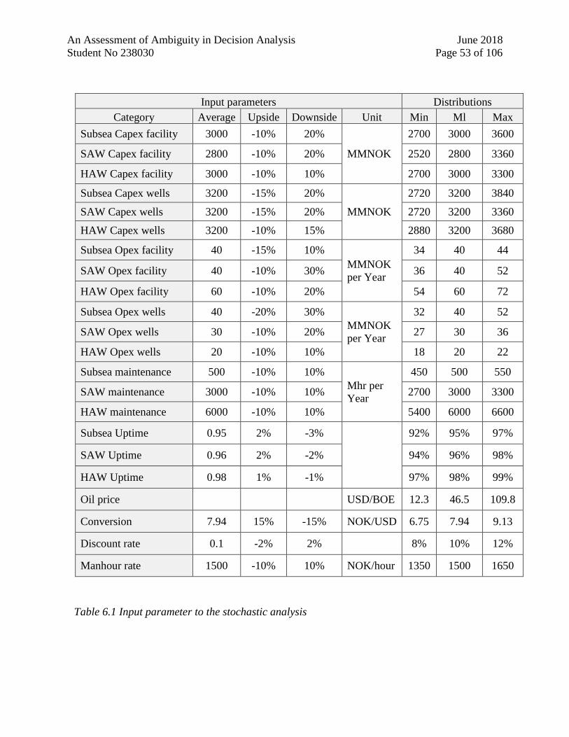
An Assessment of Ambiguity in Decision Analysis June 2018
Student No 238030 Page 53 of 106
Input parameters Distributions
Category Average Upside Downside Unit Min Ml Max
Subsea Capex facility 3000 -10% 20%
MMNOK
2700 3000 3600
SAW Capex facility 2800 -10% 20% 2520 2800 3360
HAW Capex facility 3000 -10% 10% 2700 3000 3300
Subsea Capex wells 3200 -15% 20%
MMNOK
2720 3200 3840
SAW Capex wells 3200 -15% 20% 2720 3200 3360
HAW Capex wells 3200 -10% 15% 2880 3200 3680
Subsea Opex facility 40 -15% 10%
MMNOK
per Year
34 40 44
SAW Opex facility 40 -10% 30% 36 40 52
HAW Opex facility 60 -10% 20% 54 60 72
Subsea Opex wells 40 -20% 30%
MMNOK
per Year
32 40 52
SAW Opex wells 30 -10% 20% 27 30 36
HAW Opex wells 20 -10% 10% 18 20 22
Subsea maintenance 500 -10% 10%
Mhr per
Year
450 500 550
SAW maintenance 3000 -10% 10% 2700 3000 3300
HAW maintenance 6000 -10% 10% 5400 6000 6600
Subsea Uptime 0.95 2% -3%
92% 95% 97%
SAW Uptime 0.96 2% -2% 94% 96% 98%
HAW Uptime 0.98 1% -1% 97% 98% 99%
Oil price USD/BOE 12.3 46.5 109.8
Conversion 7.94 15% -15% NOK/USD 6.75 7.94 9.13
Discount rate 0.1 -2% 2% 8% 10% 12%
Manhour rate 1500 -10% 10% NOK/hour 1350 1500 1650
Table 6.1 Input parameter to the stochastic analysis
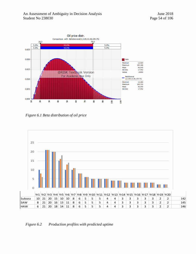
An Assessment of Ambiguity in Decision Analysis June 2018
Student No 238030 Page 54 of 106
Figure 6.1 Beta distribution of oil price
Yr1 Yr2 Yr3 Yr4 Yr5 Yr6 Yr7 Yr8 Yr9 Yr10 Yr11 Yr12 Yr13 Yr14 Yr15 Yr16 Yr17 Yr18 Yr19 Yr20
Subsea 10 21 20 15 10 10 8 6 5 5 5 4 4 3 3 3 3 3 2 2 142
SAW 8 21 20 16 13 11 8 6 5 5 5 4 4 3 3 3 3 3 2 2 145
HAW 6 21 20 18 14 11 8 6 5 5 5 4 4 3 3 3 3 3 2 2 146
0
5
10
15
20
25
Subsea SAW HAW
Figure 6.2 Production profiles with predicted uptime
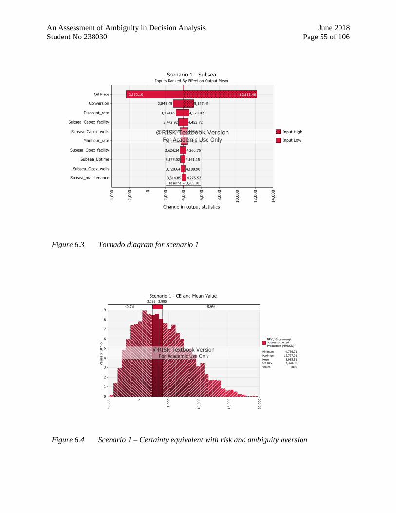
An Assessment of Ambiguity in Decision Analysis June 2018
Student No 238030 Page 55 of 106
Figure 6.3 Tornado diagram for scenario 1
Figure 6.4 Scenario 1 – Certainty equivalent with risk and ambiguity aversion
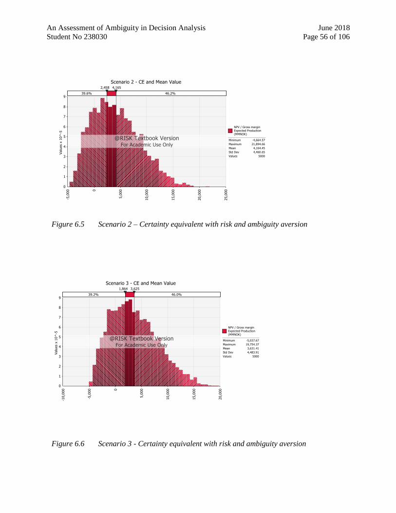
An Assessment of Ambiguity in Decision Analysis June 2018
Student No 238030 Page 56 of 106
Figure 6.6 Scenario 3 - Certainty equivalent with risk and ambiguity aversion
Figure 6.5 Scenario 2 – Certainty equivalent with risk and ambiguity aversion
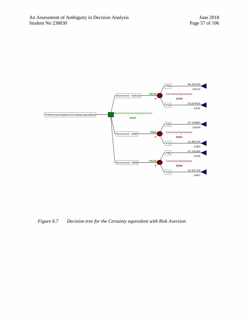
An Assessment of Ambiguity in Decision Analysis June 2018
Student No 238030 Page 57 of 106
Figure 6.7 Decision tree for the Certainty equivalent with Risk Aversion
46.9255% 0.0%
10122 10122
FALSE Certainty Equivalent
0 2439
53.0745% 0.0%
-1441 -1441
Maximise Certainty Equivalent
2562
47.1088% 47.1088%
10394 10394
TRUE Certainty Equivalent
0 2562
52.8912% 52.8912%
-1383 -1383
47.5429% 0.0%
9795 9795
FALSE Certainty Equivalent
0 2020
52.4571% 0.0%
-1967 -1967
Preference based on Certainty Equivalent
Scenario 1 - Subsea
P90
P10
Scenario 2 - SAW
P90
P10
Scenario 3 - HAW
P90
P10
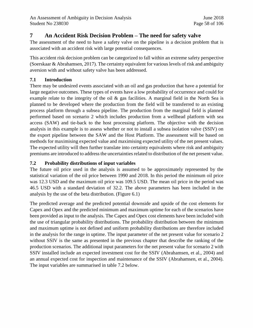
An Assessment of Ambiguity in Decision Analysis June 2018
Student No 238030 Page 58 of 106
7 An Accident Risk Decision Problem – The need for safety valve The assessment of the need to have a safety valve on the pipeline is a decision problem that is
associated with an accident risk with large potential consequences.
This accident risk decision problem can be categorized to fall within an extreme safety perspective
(Soerskaar & Abrahamsen, 2017). The certainty equivalent for various levels of risk and ambiguity
aversion with and without safety valve has been addressed.
7.1 Introduction
There may be undesired events associated with an oil and gas production that have a potential for
large negative outcomes. These types of events have a low probability of occurrence and could for
example relate to the integrity of the oil & gas facilities. A marginal field in the North Sea is
planned to be developed where the production from the field will be transferred to an existing
process platform through a subsea pipeline. The production from the marginal field is planned
performed based on scenario 2 which includes production from a wellhead platform with sea
access (SAW) and tie-back to the host processing platform. The objective with the decision
analysis in this example is to assess whether or not to install a subsea isolation valve (SSIV) on
the export pipeline between the SAW and the Host Platform. The assessment will be based on
methods for maximising expected value and maximising expected utility of the net present values.
The expected utility will then further translate into certainty equivalents where risk and ambiguity
premiums are introduced to address the uncertainties related to distribution of the net present value.
7.2 Probability distributions of input variables
The future oil price used in the analysis is assumed to be approximately represented by the
statistical variation of the oil price between 1990 and 2018. In this period the minimum oil price
was 12.3 USD and the maximum oil price was 109.5 USD. The mean oil price in the period was
46.5 USD with a standard deviation of 32.2. The above parameters has been included in the
analysis by the use of the beta distribution. (Figure 6.1)
The predicted average and the predicted potential downside and upside of the cost elements for
Capex and Opex and the predicted minimum and maximum uptime for each of the scenarios have
been provided as input to the analysis. The Capex and Opex cost elements have been included with
the use of triangular probability distributions. The probability distribution between the minimum
and maximum uptime is not defined and uniform probability distributions are therefore included
in the analysis for the range in uptime. The input parameter of the net present value for scenario 2
without SSIV is the same as presented in the previous chapter that describe the ranking of the
production scenarios. The additional input parameters for the net present value for scenario 2 with
SSIV installed include an expected investment cost for the SSIV (Abrahamsen, et al., 2004) and
an annual expected cost for inspection and maintenance of the SSIV (Abrahamsen, et al., 2004).
The input variables are summarised in table 7.2 below.
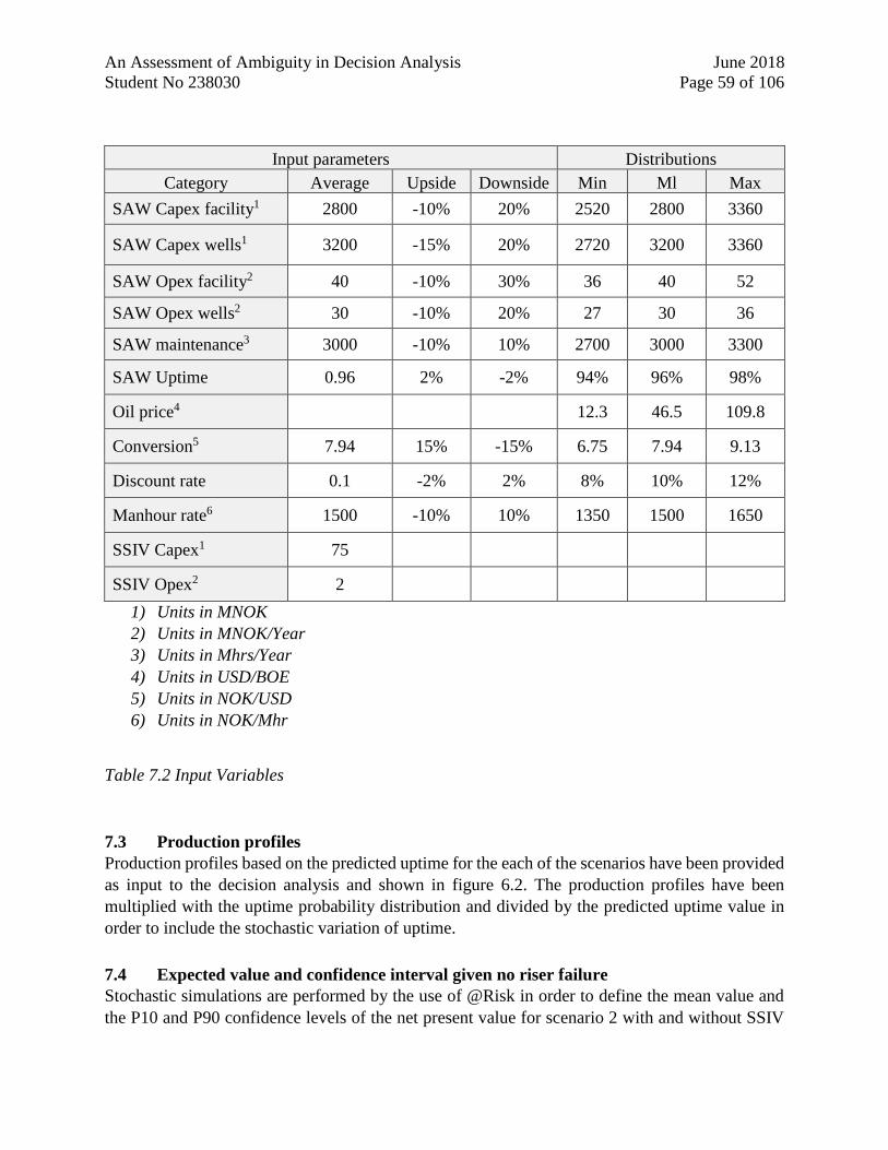
An Assessment of Ambiguity in Decision Analysis June 2018
Student No 238030 Page 59 of 106
Input parameters Distributions
Category Average Upside Downside Min Ml Max
SAW Capex facility1 2800 -10% 20% 2520 2800 3360
SAW Capex wells1 3200 -15% 20% 2720 3200 3360
SAW Opex facility2 40 -10% 30% 36 40 52
SAW Opex wells2 30 -10% 20% 27 30 36
SAW maintenance3 3000 -10% 10% 2700 3000 3300
SAW Uptime 0.96 2% -2% 94% 96% 98%
Oil price4 12.3 46.5 109.8
Conversion5 7.94 15% -15% 6.75 7.94 9.13
Discount rate 0.1 -2% 2% 8% 10% 12%
Manhour rate6 1500 -10% 10% 1350 1500 1650
SSIV Capex1 75
SSIV Opex2 2
1) Units in MNOK
2) Units in MNOK/Year
3) Units in Mhrs/Year
4) Units in USD/BOE
5) Units in NOK/USD
6) Units in NOK/Mhr
Table 7.2 Input Variables
7.3 Production profiles
Production profiles based on the predicted uptime for the each of the scenarios have been provided
as input to the decision analysis and shown in figure 6.2. The production profiles have been
multiplied with the uptime probability distribution and divided by the predicted uptime value in
order to include the stochastic variation of uptime.
7.4 Expected value and confidence interval given no riser failure
Stochastic simulations are performed by the use of @Risk in order to define the mean value and
the P10 and P90 confidence levels of the net present value for scenario 2 with and without SSIV
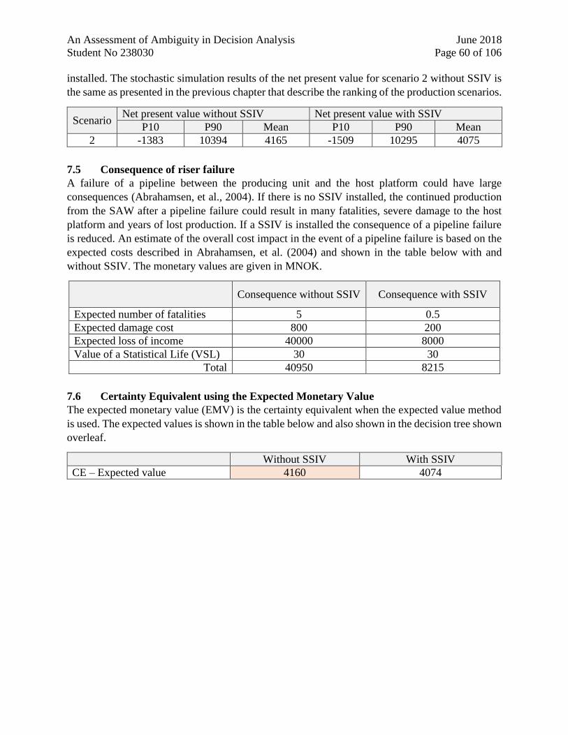
An Assessment of Ambiguity in Decision Analysis June 2018
Student No 238030 Page 60 of 106
installed. The stochastic simulation results of the net present value for scenario 2 without SSIV is
the same as presented in the previous chapter that describe the ranking of the production scenarios.
Scenario Net present value without SSIV Net present value with SSIV
P10 P90 Mean P10 P90 Mean
2 -1383 10394 4165 -1509 10295 4075
7.5 Consequence of riser failure
A failure of a pipeline between the producing unit and the host platform could have large
consequences (Abrahamsen, et al., 2004). If there is no SSIV installed, the continued production
from the SAW after a pipeline failure could result in many fatalities, severe damage to the host
platform and years of lost production. If a SSIV is installed the consequence of a pipeline failure
is reduced. An estimate of the overall cost impact in the event of a pipeline failure is based on the
expected costs described in Abrahamsen, et al. (2004) and shown in the table below with and
without SSIV. The monetary values are given in MNOK.
Consequence without SSIV Consequence with SSIV
Expected number of fatalities 5 0.5
Expected damage cost 800 200
Expected loss of income 40000 8000
Value of a Statistical Life (VSL) 30 30
Total 40950 8215
7.6 Certainty Equivalent using the Expected Monetary Value
The expected monetary value (EMV) is the certainty equivalent when the expected value method
is used. The expected values is shown in the table below and also shown in the decision tree shown
overleaf.
Without SSIV With SSIV
CE – Expected value 4160 4074
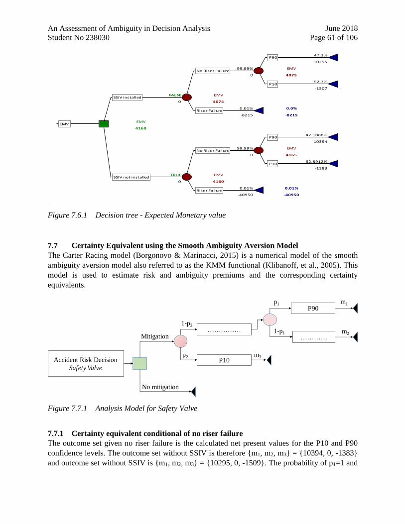
An Assessment of Ambiguity in Decision Analysis June 2018
Student No 238030 Page 61 of 106
Figure 7.6.1 Decision tree - Expected Monetary value
7.7 Certainty Equivalent using the Smooth Ambiguity Aversion Model
The Carter Racing model (Borgonovo & Marinacci, 2015) is a numerical model of the smooth
ambiguity aversion model also referred to as the KMM functional (Klibanoff, et al., 2005). This
model is used to estimate risk and ambiguity premiums and the corresponding certainty
equivalents.
Figure 7.7.1 Analysis Model for Safety Valve
7.7.1 Certainty equivalent conditional of no riser failure
The outcome set given no riser failure is the calculated net present values for the P10 and P90
confidence levels. The outcome set without SSIV is therefore {m1, m2, m3} = {10394, 0, -1383}
and outcome set without SSIV is {m1, m2, m3} = {10295, 0, -1509}. The probability of p1=1 and
47.3% 0.0%
10295 10295.01185
99.99% EMV
0 4075
52.7% 0.0%
-1507 -1506.889975
FALSE EMV
0 4074
0.01% 0.0%
-8215 -8215
EMV
4160
47.1088% 47.1041%
10394 10394
99.99% EMV
0 4165
52.8912% 52.8859%
-1383 -1383
TRUE EMV
0 4160
0.01% 0.01%
-40950 -40950
EMV
SSIV installed
Riser Failure
No Riser Failure
P90
P10
SSIV not installed
Riser Failure
No Riser Failure
P90
P10
……………
P10
P90
…………
p2
1-p2
p1
1-p1Mitigation
No mitigation
m1
m2
m3Accident Risk Decision
Safety Valve
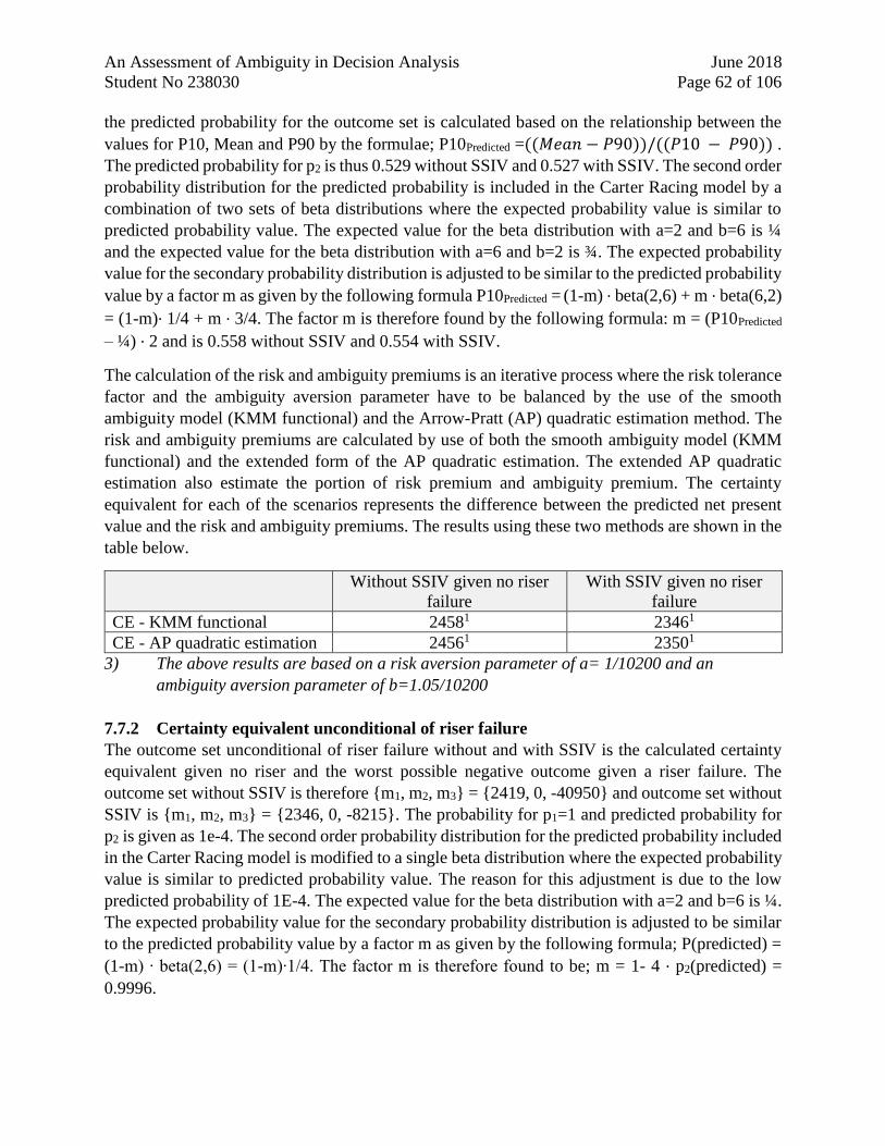
An Assessment of Ambiguity in Decision Analysis June 2018
Student No 238030 Page 62 of 106
the predicted probability for the outcome set is calculated based on the relationship between the
values for P10, Mean and P90 by the formulae; P10Predicted =((𝑀𝑒𝑎𝑛 − 𝑃90))/((𝑃10 − 𝑃90)) .
The predicted probability for p2 is thus 0.529 without SSIV and 0.527 with SSIV. The second order
probability distribution for the predicted probability is included in the Carter Racing model by a
combination of two sets of beta distributions where the expected probability value is similar to
predicted probability value. The expected value for the beta distribution with a=2 and b=6 is ¼
and the expected value for the beta distribution with a=6 and b=2 is ¾. The expected probability
value for the secondary probability distribution is adjusted to be similar to the predicted probability
value by a factor m as given by the following formula P10Predicted = (1-m) ∙ beta(2,6) + m ∙ beta(6,2)
= (1-m)∙ 1/4 + m ∙ 3/4. The factor m is therefore found by the following formula: m = (P10Predicted
– ¼) ∙ 2 and is 0.558 without SSIV and 0.554 with SSIV.
The calculation of the risk and ambiguity premiums is an iterative process where the risk tolerance
factor and the ambiguity aversion parameter have to be balanced by the use of the smooth
ambiguity model (KMM functional) and the Arrow-Pratt (AP) quadratic estimation method. The
risk and ambiguity premiums are calculated by use of both the smooth ambiguity model (KMM
functional) and the extended form of the AP quadratic estimation. The extended AP quadratic
estimation also estimate the portion of risk premium and ambiguity premium. The certainty
equivalent for each of the scenarios represents the difference between the predicted net present
value and the risk and ambiguity premiums. The results using these two methods are shown in the
table below.
Without SSIV given no riser
failure
With SSIV given no riser
failure
CE - KMM functional 24581 23461
CE - AP quadratic estimation 24561 23501
3) The above results are based on a risk aversion parameter of a= 1/10200 and an
ambiguity aversion parameter of b=1.05/10200
7.7.2 Certainty equivalent unconditional of riser failure
The outcome set unconditional of riser failure without and with SSIV is the calculated certainty
equivalent given no riser and the worst possible negative outcome given a riser failure. The
outcome set without SSIV is therefore {m1, m2, m3} = {2419, 0, -40950} and outcome set without
SSIV is {m1, m2, m3} = {2346, 0, -8215}. The probability for p1=1 and predicted probability for
p2 is given as 1e-4. The second order probability distribution for the predicted probability included
in the Carter Racing model is modified to a single beta distribution where the expected probability
value is similar to predicted probability value. The reason for this adjustment is due to the low
predicted probability of 1E-4. The expected value for the beta distribution with a=2 and b=6 is ¼.
The expected probability value for the secondary probability distribution is adjusted to be similar
to the predicted probability value by a factor m as given by the following formula; P(predicted) =
(1-m) ∙ beta(2,6) = (1-m)∙1/4. The factor m is therefore found to be; m = 1- 4 ∙ p2(predicted) =
0.9996.
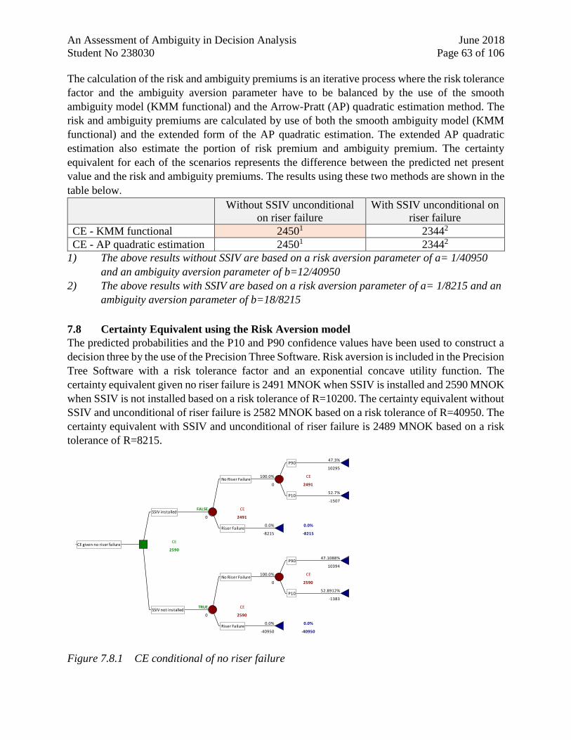
An Assessment of Ambiguity in Decision Analysis June 2018
Student No 238030 Page 63 of 106
The calculation of the risk and ambiguity premiums is an iterative process where the risk tolerance
factor and the ambiguity aversion parameter have to be balanced by the use of the smooth
ambiguity model (KMM functional) and the Arrow-Pratt (AP) quadratic estimation method. The
risk and ambiguity premiums are calculated by use of both the smooth ambiguity model (KMM
functional) and the extended form of the AP quadratic estimation. The extended AP quadratic
estimation also estimate the portion of risk premium and ambiguity premium. The certainty
equivalent for each of the scenarios represents the difference between the predicted net present
value and the risk and ambiguity premiums. The results using these two methods are shown in the
table below.
Without SSIV unconditional
on riser failure
With SSIV unconditional on
riser failure
CE - KMM functional 24501 23442
CE - AP quadratic estimation 24501 23442
1) The above results without SSIV are based on a risk aversion parameter of a= 1/40950
and an ambiguity aversion parameter of b=12/40950
2) The above results with SSIV are based on a risk aversion parameter of a= 1/8215 and an
ambiguity aversion parameter of b=18/8215
7.8 Certainty Equivalent using the Risk Aversion model
The predicted probabilities and the P10 and P90 confidence values have been used to construct a
decision three by the use of the Precision Three Software. Risk aversion is included in the Precision
Tree Software with a risk tolerance factor and an exponential concave utility function. The
certainty equivalent given no riser failure is 2491 MNOK when SSIV is installed and 2590 MNOK
when SSIV is not installed based on a risk tolerance of R=10200. The certainty equivalent without
SSIV and unconditional of riser failure is 2582 MNOK based on a risk tolerance of R=40950. The
certainty equivalent with SSIV and unconditional of riser failure is 2489 MNOK based on a risk
tolerance of R=8215.
Figure 7.8.1 CE conditional of no riser failure
47.3% 0.0%
10295 10295.01185
100.0% CE
0 2491
52.7% 0.0%
-1507 -1506.889975
FALSE CE
0 2491
0.0% 0.0%
-8215 -8215
CE
2590
47.1088% 47.1088%
10394 10394
100.0% CE
0 2590
52.8912% 52.8912%
-1383 -1383
TRUE CE
0 2590
0.0% 0.0%
-40950 -40950
CE given no riser failure
SSIV installed
Riser Failure
No Riser Failure
P90
P10
SSIV not installed
Riser Failure
No Riser Failure
P90
P10
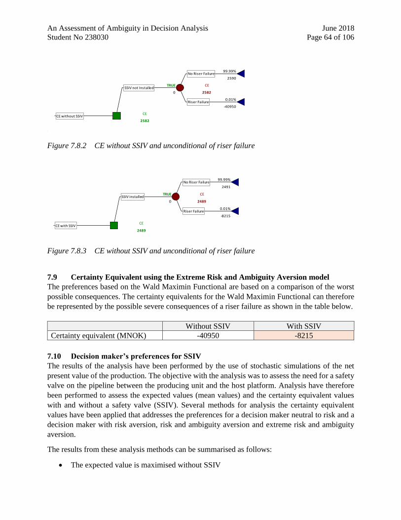
An Assessment of Ambiguity in Decision Analysis June 2018
Student No 238030 Page 64 of 106
Figure 7.8.2 CE without SSIV and unconditional of riser failure
Figure 7.8.3 CE without SSIV and unconditional of riser failure
7.9 Certainty Equivalent using the Extreme Risk and Ambiguity Aversion model
The preferences based on the Wald Maximin Functional are based on a comparison of the worst
possible consequences. The certainty equivalents for the Wald Maximin Functional can therefore
be represented by the possible severe consequences of a riser failure as shown in the table below.
Without SSIV With SSIV
Certainty equivalent (MNOK) -40950 -8215
7.10 Decision maker’s preferences for SSIV
The results of the analysis have been performed by the use of stochastic simulations of the net
present value of the production. The objective with the analysis was to assess the need for a safety
valve on the pipeline between the producing unit and the host platform. Analysis have therefore
been performed to assess the expected values (mean values) and the certainty equivalent values
with and without a safety valve (SSIV). Several methods for analysis the certainty equivalent
values have been applied that addresses the preferences for a decision maker neutral to risk and a
decision maker with risk aversion, risk and ambiguity aversion and extreme risk and ambiguity
aversion.
The results from these analysis methods can be summarised as follows:
The expected value is maximised without SSIV
99.99% 99.99%
2491 2490.804768
TRUE CE
0 2489
0.01% 0.01%
-8215 -8215
CE
2489CE with SSIV
SSIV installed
Riser Failure
No Riser Failure
99.99% 99.99%
2590 2589.979069
TRUE CE
0 2582
0.01% 0.01%
-40950 -40950
CE
2582CE without SSIV
SSIV not Installed
Riser Failure
No Riser Failure
An Assessment of Ambiguity in Decision Analysis June 2018
Student No 238030 Page 65 of 106
The risk and ambiguity averse certainty equivalent is maximised without SSIV
The risk averse certainty equivalent is maximised without SSIV
The maximum worst consequence is minimised with SSIV
A risk neutral decision maker will have a preference to not have SSIV since expected value is
highest for this alternative. A risk and ambiguity averse decision maker will have a preference to
not have a SSIV since the certainty equivalent for the KMM functional and Arrow-Pratt
Approximation is highest for this alternative. A risk averse decision maker will there also have a
preference to not have a SSIV since the certainty equivalent calculated by use of the Precision Tree
software is highest without SSIV. The ALARP principle however states that a safety measure has
to be implemented unless it can be demonstrated that there is a gross disproportion between the
cost and the benefit. I.e. that the expected cost of implementation is much larger than the expected
benefit. The
An extreme risk and ambiguity decision maker will however have a preference for the alternative
with SSIV since the maximum worst consequence is minimised for this alternative.
An Assessment of Ambiguity in Decision Analysis June 2018
Student No 238030 Page 66 of 106
8 Analysis and discussions As shown by the previous examples, there are theoretical models for decision analysis with
ambiguity that can be used to analyse several types of decision problems that the industry faces.
It is however a concern that the industry do not seem to be aware of these theoretical models.
Theoretical models for decision analysis with ambiguity are also not included in the textbooks
currently used in the lecturing of decision analysis. Models of risk aversion and calculation of
corresponding certainty equivalent values are covered in the decision analysis textbook “Practical
Management Science” by Winston & Albright (2018), although ambiguity and ambiguity aversion
is not covered. It is also stated in Winston & Albright (2018) that the concept of risk aversion and
certainty equivalent is rarely used in the industry. In the text book “Making good decision” by
Bratvold & Begg (2009), the concept of risk aversion and certainty equivalent is very briefly
mentioned. In the papers (Abrahamsen, et al., 2004), (Abrahamsen & Aven, 2008), (Soerskaar &
Abrahamsen, 2017) used in the course RIS620 “Economic analysis in Risk Management” there is
also no description given of theoretical models associated with ambiguity. The theoretical models
for decision analysis with ambiguity do therefore neither seem to be known nor aligned among
peers of experts within the field of decision theory. Further research on the practical applications
of the theoretical models represented by the Smooth Ambiguity Functional (Klibanoff, et al., 2005)
and the Extended Arrow-Pratt Quadratic Estimation (Maccheroni, et al., 2013) should therefore be
done at several institutions in order to have these theories accepted and included in decision
analysis textbooks. This is a challenge that I believe needs to be resolved in order to introduce
quantitative models for decision analysis with ambiguity to the industry.
The balance between normative decision theory and decision making practice, how the decision
problems that are analysed can be framed in an uncertainty perspective and how these perspectives
can assist in rational decision making are further discussed in the subsections.
8.1 Decision theory versus decision making practice
Relevant models considered to be used to define decision maker’s preferences under risk and
ambiguity have been assessed with reference to a three-color decision problem (Ellsberg, 1961).
The decision theoretical models that the decision maker can use to find his preferences in the three-
color decision problem were found to be the Smooth Ambiguity Functional (Klibanoff, et al.,
2005), the Extended Arrow-Pratt Quadratic Estimation (Maccheroni, et al., 2013) and the Wald
Maximin Functional (Wald, 1949).
Qualitative research of decision making practice have been performed with reference to a selected
peer group that have project management functions within the oil and gas industry. The objective
with the qualitative research was to assess if the decision theory under ambiguity is known and
used by the industry. The responses indicate that the decision theory under ambiguity and the use
of certainty equivalent, risk premiums and ambiguity premiums are generally not known by the
members of the peer group. Findings from the case studies in the qualitative research do however
seem to correspond with previous findings (Kahneman & Tversky, 1992) that decision makers
have a tendency to think differently about positive and negative outcomes. The decision maker
An Assessment of Ambiguity in Decision Analysis June 2018
Student No 238030 Page 67 of 106
may have a tendency to a risk seeking and ambiguity neutral behavior towards negative outcomes
and a tendency to a risk and ambiguity averse behavior for positive outcomes.
The normative decision theory under ambiguity (Klibanoff, et al., 2005), (Maccheroni, et al.,
2013), (Wald, 1949) is based on risk and ambiguity aversion. The preference found by the use of
the normative decision theory would therefore provide guidance to the decision maker, since risk
and ambiguity aversion are introduced for both positive and negative outcomes.
8.2 Decision analysis of business risk
The analytical methods of the Smooth Ambiguity Functional (Klibanoff, et al., 2005), the
Extended Arrow-Pratt Quadratic Estimation (Maccheroni, et al., 2013) and the Wald Maximin
Functional (Wald, 1949) have been documented by a stylized business risk decision problem. The
business risk decision problem is whether to run or withdraw from a race. The analysis shows that
a risk neutral decision is to run, while a risk and ambiguity averse decision and an extreme risk
and ambiguity averse decision is to withdraw.
An oil company are sometimes faced with similar business risk decision problems as illustrated by
the Carter racing dilemma. These decisions could be related to the trade-off between the selection
of a familiar Norwegian fabrication yard or an unknown foreign fabrication yard. The business
risk decision could also be related to the trade-off between onshore and offshore execution of the
mechanical completion of a platform. Following the logic from the Carter racing, a risk neutral
decision would be to select the alternative with the lowest cost estimate and shortest delivery,
while a risk and ambiguity averse decision would be to select the alternative with the highest
predictability of cost and schedule.
8.3 Decision analysis of cost risk
The research results indicate that project contingency is used as a way to account for uncertainties
in project cost estimates. Project contingency is thus a similar concept as risk and ambiguity
premiums for an uncertainty associated with cost risk. The decision makers perform a cost risk
assessment of the uncertainty range or confidence interval and assigns a margin on top of the base
estimate based on qualitative assessments. The research results indicate that there are differences
in how project contingency is introduced in a project cost estimate. The project contingency is
either included as an deterministic margin in the P50 confidence level or the project contingency
is introduced by a qualitative judgment of the uncertainty range. The difference between the P70
confidence level and the P50 confidence level is normally used as the project contingency in cases
where an uncertainty range or confidence interval is defined. To have project contingency as the
difference between the P70 confidence level and the P50 confidence level is also in alignment with
the analysis performed in the project contingency example by the use of the Smooth Ambiguity
Functional and the Extended Arrow-Pratt Quadratic Estimation method.
8.4 Decision analysis of production risk
The responses from the in-depth interviews indicate that the P10, P50 and P90 confidence levels
are used as the decision parameters for the production risk related to the income prognosis of an
oil and gas production. It is however not clear from the responses how the confidence levels are
used to define a margin or buffer in the value proposition for the income prognosis.
An Assessment of Ambiguity in Decision Analysis June 2018
Student No 238030 Page 68 of 106
In the production risk example, the net present value of three alternative project development
scenarios are compared. The production profiles provided for these scenarios are based on
expected annual production. Information of the uncertainty range for the expected annual
production is not defined. The analysis for the production risk example do therefore not include
the uncertainties associated with the subsurface performance.
Stochastic analysis has been performed on the variation in Capex, Opex and uptime in order to
define the 80% confidence interval for the net present value for the three scenarios. The uncertainty
range represented by the 80% confidence interval have been analysed in order to define the
preference based on the certainty equivalent. The analysis shows that a wellhead platform with sea
access (SAW) is the overall preferred alternative as this gives the highest certainty equivalent both
for a risk neutral decision maker (expected value), for a decision maker with risk aversion
(Precision tree) and for a decision maker with risk and ambiguity aversion (Smooth Ambiguity
Functional/Extended Arrow-Pratt Quadratic Estimation Method).
This production risk decision problem of ranking of different concepts do show the benefit of
having a single equivalent value (certainty equivalent) to compare. To perform ranking of the
concepts based on the expected value and the uncertainty range could also be done, but would
most likely be based on a qualitative judgement of the uncertainty range.
8.5 Decision analysis of accidental risk
The responses from the in-depth interviews indicate that impact assessments are used for decision
problems that relates to accident risk. An example of a decision problem associated with accident
risk is whether or not to install a SSIV on the pipeline between the wellhead platform and the host
platform. The second order probability distribution defined by the two beta distributions for the
Smooth Ambiguity Functional do not work when the probability of riser failure is as low as 1E-4.
The preferences for this type of accident risk can however be defined by the use of the Wald
Maximin Functional (Wald, 1949). To install a SSIV is therefore the preferred alternative as this
gives the highest certainty equivalent for the extreme undesired event. There is also a relatively
small difference in the expected net present value with and without SSIV. The expected cost with
SSIV is therefore not in gross disproportion to the benefit gained. A SSIV should therefore be
installed to satisfy the ALARP principle that states that a safety measure is to be installed unless
it can be demonstrated that the expected cost is grossly disproportionate to the benefit gained
(Soerskaar & Abrahamsen, 2017).
8.6 Use of risk aversion models
The decision problems were also analysed by the risk aversion model included in the Precision
Tree software provided by Palisade Ltd. This risk aversion model refers to the subjective expected
utility and do not include ambiguity aversion. In the decision problems for business risk, the risk
aversion model gave the same preference as the expected value method. In the cost risk decision
problem, the risk averse model would include a project contingency equivalent to the difference
between the P62 confidence level and the P50 confidence level. This project contingency is lower
than recommended practice. The risk aversion model seem to capture only part of uncertainty in
these decision problems. These cost risk and business risk decision problems are therefore not
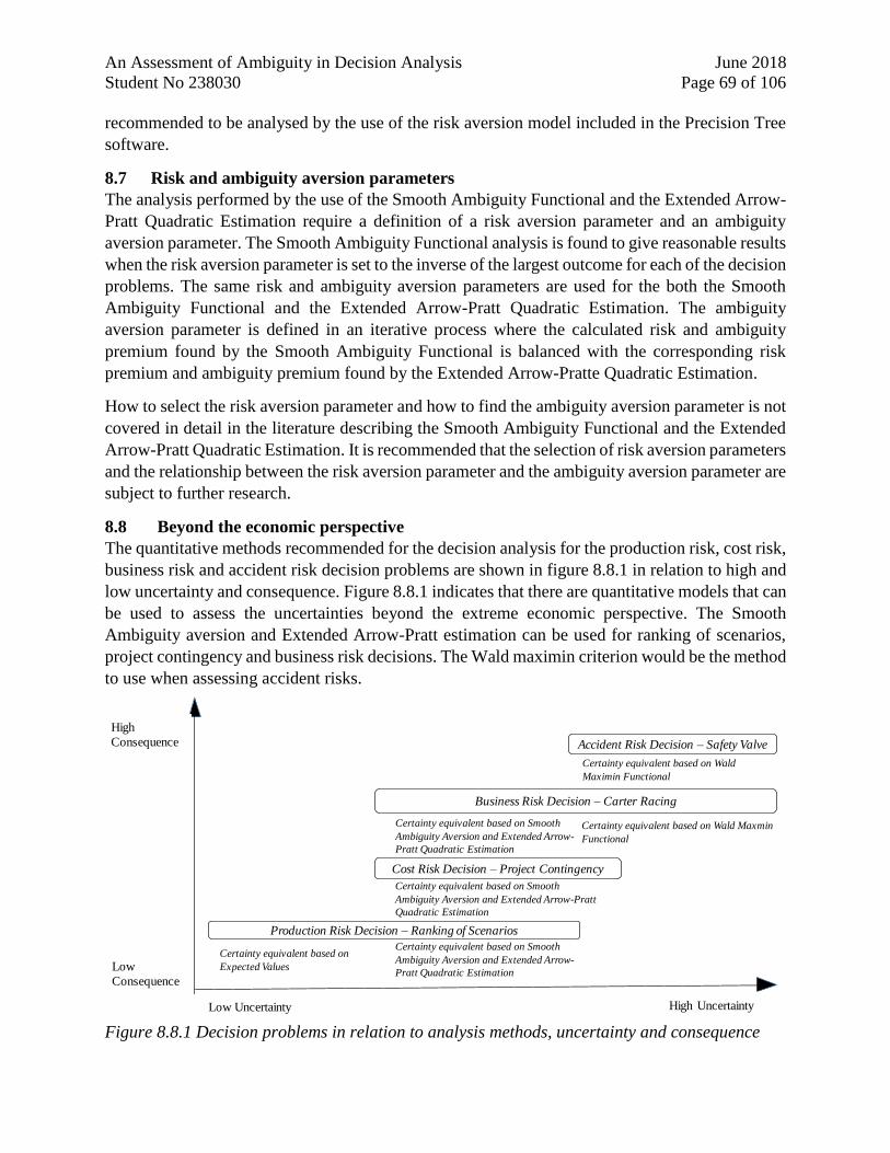
An Assessment of Ambiguity in Decision Analysis June 2018
Student No 238030 Page 69 of 106
recommended to be analysed by the use of the risk aversion model included in the Precision Tree
software.
8.7 Risk and ambiguity aversion parameters
The analysis performed by the use of the Smooth Ambiguity Functional and the Extended Arrow-
Pratt Quadratic Estimation require a definition of a risk aversion parameter and an ambiguity
aversion parameter. The Smooth Ambiguity Functional analysis is found to give reasonable results
when the risk aversion parameter is set to the inverse of the largest outcome for each of the decision
problems. The same risk and ambiguity aversion parameters are used for the both the Smooth
Ambiguity Functional and the Extended Arrow-Pratt Quadratic Estimation. The ambiguity
aversion parameter is defined in an iterative process where the calculated risk and ambiguity
premium found by the Smooth Ambiguity Functional is balanced with the corresponding risk
premium and ambiguity premium found by the Extended Arrow-Pratte Quadratic Estimation.
How to select the risk aversion parameter and how to find the ambiguity aversion parameter is not
covered in detail in the literature describing the Smooth Ambiguity Functional and the Extended
Arrow-Pratt Quadratic Estimation. It is recommended that the selection of risk aversion parameters
and the relationship between the risk aversion parameter and the ambiguity aversion parameter are
subject to further research.
8.8 Beyond the economic perspective
The quantitative methods recommended for the decision analysis for the production risk, cost risk,
business risk and accident risk decision problems are shown in figure 8.8.1 in relation to high and
low uncertainty and consequence. Figure 8.8.1 indicates that there are quantitative models that can
be used to assess the uncertainties beyond the extreme economic perspective. The Smooth
Ambiguity aversion and Extended Arrow-Pratt estimation can be used for ranking of scenarios,
project contingency and business risk decisions. The Wald maximin criterion would be the method
to use when assessing accident risks.
Figure 8.8.1 Decision problems in relation to analysis methods, uncertainty and consequence
High
Consequence
Low
Consequence
High UncertaintyLow Uncertainty
Business Risk Decision – Carter Racing
Accident Risk Decision – Safety Valve
Production Risk Decision – Ranking of Scenarios
Cost Risk Decision – Project Contingency
Certainty equivalent based on
Expected Values
Certainty equivalent based on Smooth
Ambiguity Aversion and Extended Arrow-
Pratt Quadratic Estimation
Certainty equivalent based on Smooth
Ambiguity Aversion and Extended Arrow-Pratt
Quadratic Estimation
Certainty equivalent based on Smooth
Ambiguity Aversion and Extended Arrow-
Pratt Quadratic Estimation
Certainty equivalent based on Wald Maxmin
Functional
Certainty equivalent based on Wald
Maximin Functional
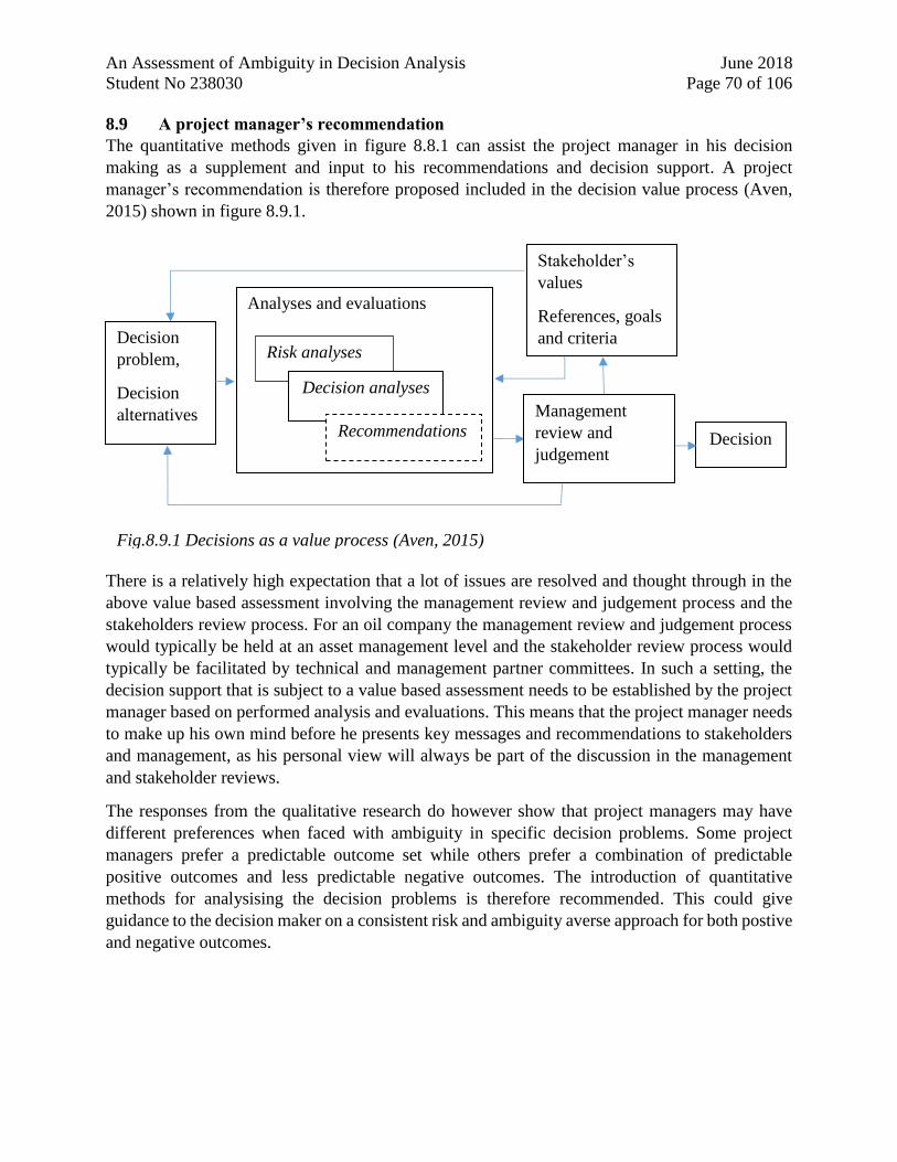
An Assessment of Ambiguity in Decision Analysis June 2018
Student No 238030 Page 70 of 106
8.9 A project manager’s recommendation
The quantitative methods given in figure 8.8.1 can assist the project manager in his decision
making as a supplement and input to his recommendations and decision support. A project
manager’s recommendation is therefore proposed included in the decision value process (Aven,
2015) shown in figure 8.9.1.
There is a relatively high expectation that a lot of issues are resolved and thought through in the
above value based assessment involving the management review and judgement process and the
stakeholders review process. For an oil company the management review and judgement process
would typically be held at an asset management level and the stakeholder review process would
typically be facilitated by technical and management partner committees. In such a setting, the
decision support that is subject to a value based assessment needs to be established by the project
manager based on performed analysis and evaluations. This means that the project manager needs
to make up his own mind before he presents key messages and recommendations to stakeholders
and management, as his personal view will always be part of the discussion in the management
and stakeholder reviews.
The responses from the qualitative research do however show that project managers may have
different preferences when faced with ambiguity in specific decision problems. Some project
managers prefer a predictable outcome set while others prefer a combination of predictable
positive outcomes and less predictable negative outcomes. The introduction of quantitative
methods for analysising the decision problems is therefore recommended. This could give
guidance to the decision maker on a consistent risk and ambiguity averse approach for both postive
and negative outcomes.
Analyses and evaluations
Risk analyses
Decision
problem,
Decision
alternatives
Stakeholder’s
values
References, goals
and criteria
Decision
Decision analyses
Fig.8.9.1 Decisions as a value process (Aven, 2015)
Recommendations
Management
review and
judgement
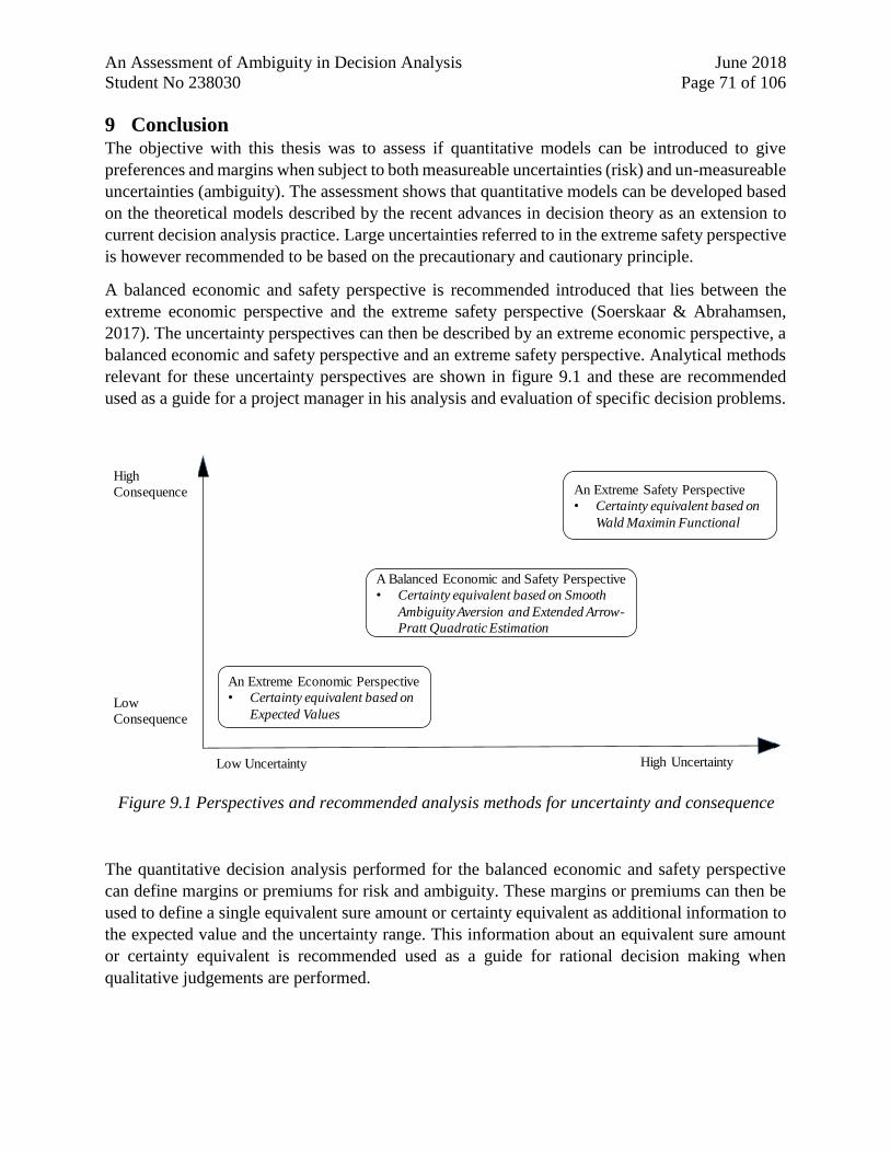
An Assessment of Ambiguity in Decision Analysis June 2018
Student No 238030 Page 71 of 106
9 Conclusion The objective with this thesis was to assess if quantitative models can be introduced to give
preferences and margins when subject to both measureable uncertainties (risk) and un-measureable
uncertainties (ambiguity). The assessment shows that quantitative models can be developed based
on the theoretical models described by the recent advances in decision theory as an extension to
current decision analysis practice. Large uncertainties referred to in the extreme safety perspective
is however recommended to be based on the precautionary and cautionary principle.
A balanced economic and safety perspective is recommended introduced that lies between the
extreme economic perspective and the extreme safety perspective (Soerskaar & Abrahamsen,
2017). The uncertainty perspectives can then be described by an extreme economic perspective, a
balanced economic and safety perspective and an extreme safety perspective. Analytical methods
relevant for these uncertainty perspectives are shown in figure 9.1 and these are recommended
used as a guide for a project manager in his analysis and evaluation of specific decision problems.
Figure 9.1 Perspectives and recommended analysis methods for uncertainty and consequence
The quantitative decision analysis performed for the balanced economic and safety perspective
can define margins or premiums for risk and ambiguity. These margins or premiums can then be
used to define a single equivalent sure amount or certainty equivalent as additional information to
the expected value and the uncertainty range. This information about an equivalent sure amount
or certainty equivalent is recommended used as a guide for rational decision making when
qualitative judgements are performed.
High
Consequence
Low
Consequence
High UncertaintyLow Uncertainty
An Extreme Safety Perspective
• Certainty equivalent based on
Wald Maximin Functional
An Extreme Economic Perspective
• Certainty equivalent based on
Expected Values
A Balanced Economic and Safety Perspective
• Certainty equivalent based on Smooth
Ambiguity Aversion and Extended Arrow-
Pratt Quadratic Estimation
An Assessment of Ambiguity in Decision Analysis June 2018
Student No 238030 Page 72 of 106
10 References
Abrahamsen, E. B. & Aven, T., 2008. On the consistency of riks acceptance with normative
theories for decision-making. Reliability Engineering and System Safety, Volume 93, pp. 1906-
1910.
Abrahamsen, E. B., Vinnem, J. E. & Wiencke, H. S., 2004. Safety management and the use of
exppected values. Risk Decision and Policy, Volume 9, pp. 347-357.
Aerts, D. & Sozzo, S., 2015. From Ambiguity Aversion to a Generalized Expected Utiltity.
Modeling Preferences in a Quantum Probabilistic Framework, s.l.: s.n.
Anscombe, F. J. & Aumann, R. J., 1963. A definition of Subjective Probability. The Annals of
Mathematical Statistics, 34(1), pp. 199-205.
ASTM-E1369, 2015. Standard Guide for Selecting Techniques for Treating Uncertainty and
Risk in the Economic Evaluation of Buildings and Buidling Systems. s.l.:ASTM.
ASTM-E1946, 2012. Standard Practice for Measuring Cost Risk of Buildings and Buidling
Systems and Other Constructed Projects. s.l.:ASTM.
ASTM-E2168, 2016. Standard Classification for Allowance, Contingency, and Reserve Sums in
Building Construction Estimating. s.l.:ASTM International.
Aven, T., 2012. Foundations of Risk Analysis. 2 ed. s.l.:Wiley.
Aven, T., 2014. Risk, Surprises and Black Swans. 1 ed. s.l.:Routledge.
Aven, T., 2015. Risk analysis. 2 ed. s.l.:Wiley.
Aven, T., 2015. Risk Analysis. 2 ed. s.l.:Wiley.
Aven, T., Baraldi, P., Flage, R. & Zio, E., 2014. Uncertainty in Risk Assessments. 1 ed.
s.l.:Wiley.
Baccelli, J., 2017. Risk attitudes in axiomatic decision theory: a conceptual perspective, Munich,
Germany: Springer.
Borgonovo, E., Cappelli, V., Maccheroni, F. & Marinacci, M., 2015. Risk analysis and decision
theory: Foundations, s.l.: Working Paper No. 556.
Borgonovo, E., Cappelli, V., Maccheroni, F. & Marinacci, M., 2016. Model Uncertainty in Risk
Analysis and Decison Theory: A Preliminary Investigation, s.l.: Working Paper n. 592.
Borgonovo, E., Cappelli, V., Maccheroni, F. & Marinacci, M., 2018. Risk analysis and decision
theory: A bridge. European Journal of Operational Research, 264(1 July 2017), pp. 280-293.
Borgonovo, E. & Marinacci, M., 2015. Decision analysis under ambiguity. European Journal of
Operational Research, pp. 823-836.
An Assessment of Ambiguity in Decision Analysis June 2018
Student No 238030 Page 73 of 106
Borgonovo, E. & Marinacci, M., 2015. Decision analysis under ambiguity. European Journal of
Operational Research, 7 February.pp. 823-836.
Bradley, R., 2015. Ellsberg's Paradox and the Value of Chances. 17 March, pp. 1-16.
Bratvold, R. B. & Begg, S. H., 2009. Making Good Decisions. 222 Palisades Creek Drive:
Society of Petroleum Engineers.
Brittain, J. & Sitkin, S. B., 1990. Facts, Figures and Organizational Decisions: Carter Racing and
Quantitative Analysis in the Organizational Behavior Classroom. Journal of Management
Education, 14(1), pp. 62-81.
Burger, R., 2003. Contingency, Quantifying the Uncertainty. Cost Engineering, 45(No. 8,
August 2003), pp. 12-17.
Cerreia-Vioglio, S., Maccheroni, F., Marinacci, M. & Montrucchio, L., 2013a. Ambiguity and
robust statistics. Journal of Economic Theory, 148, pp. 974-1049.
Chow, C. V., Arnondin, K. D. & Ballard, N. D., 2000. Managing risks using integrated
production models: applications. SPE 57473, pp. 94-98.
Chow, C. V. & Arnondin, M. C., 2000. Managing risks using integrated production models:
process description. SPE 57472, pp. 54-57.
Dillon, R. L., John, R. & Winterfeldt, D. v., 2002. Assessment of Cost Uncertainties for Large
Technology Project: A Methodology and an Application. Interfaces, 32(No. 4, July-August
2002), pp. 52-66.
dos Santos, L., Destefano, N. & Martinez, A. S., 2018. Decision making generalized by a
cumulative probability weighting function. Physica A, 490(25 August 2017), pp. 250-259.
Eichberger, J. & Kelsey, D., 2007. Chapter V: Ambiguity. In: The Oxford Handbook of Rational
and Social Choice. s.l.:s.n., pp. 1-11.
Ellsberg, D., 1961. Risk, ambiguity and the Savage axioms.. Quarterly Journal of Economics,
75(4), pp. 643-669.
Etner, J., Jeleva, M. & Tallon, J.-M., 2012. Decision Theory under Ambiguity. Issue Vol. 26, pp.
234-270.
Fassihi, M. R., Blinten, J. S. & Riis, T., 2000. Risk managment for offshore-prospect
development. SPE 52975, pp. 43-44.
Gilboa, I. & Marinacci, M., 2011. Ambiguity and the Bayesian Paradigm. 12 April, pp. 1-70.
Gilboa, I. & Schmeidler, D., 1989. Maxmin expected utility with non-unique prior. Journal of
Mathematical Economics, Volume 97, pp. 141-153.
Grant, S. & van Zandt, T., 2007. Expected Utility Theory, Fontainebleau, France: INSEAD The
Business School for the World.
An Assessment of Ambiguity in Decision Analysis June 2018
Student No 238030 Page 74 of 106
Hampel, F., 2009. Nonadditive Probabilities in Statistics. Journal of Statistical Theory and
Practice, 3(No. 1, March 2009), pp. 1-23.
Hansen, L. P. & Marinacci, M., 2016. Ambiguity Aversion and Model Misspecification: An
Economic Perspective. Statistical Science, 31(4), pp. 511-515.
Howard, R. A., 1988. Decision analysis: Practice and Promise. Management Science, 34(6), pp.
679-695.
Howell, D., Windahl, C. & Seidel, R., 2010. A project contingency framework based on
uncertainity and its consequences. International Journal of Project Management, 28(9 June
2009), pp. 256-264.
Idrus, A., Nuruddin, M. F. & Rohman, M. A., 2011. Development of project cost contingency
estimation model using risk analysis and fuzzy expert system. Expert Systems with Applications,
Volume 38, pp. 1501-1508.
Kahneman, D. & Tversky, A., 1992. Advances in Prospect Theory: Cumulative Representation
of Uncertainity. Journal of Risk and Uncertainty, Volume 5, pp. 297-323.
Kaplan, S. & Garrick, B., 1981. On the quantiative definition of risk. Risk Analysis 17, pp. 407-
417.
Karlsen, J. T. & Lereim, J., 2005. Management of Project Contingency and Allowance. Cost
Engineering, 47(No. 9, September 2005), pp. 24-29.
Klibanoff, P., Marinacci, M. & Mukeri, S., 2005. A smooth model of decision making under
ambiguity. Economics, 73(6), pp. 1849-1892.
Klibanoff, P., Marinacci, M. & Mukeri, S., 2005. A smooth model of decision making under
ambiguity. Econometria, Vol. 73, No. 6, pp. 1849-1892.
Klibanoff, P., Marinacci, M. & Mukeri, S., 2012. On the smooth ambiguity model: A Reply.
Econometrica, 80(No. 3, May 2012), pp. 1303-1321.
Liedtka, J., 1990. The Challenger Launch Decision: Case and Teaching Note. Int. J. Value Based
Management, 3(1), pp. 29-41.
Lindley, D., 1985. Making Decisions. 2 ed. s.l.:John Wiley & Sons.
Maccheroni, F., Marinacci, M. & Ruffino, D., 2013. Alpha as ambiguity: Robust Mean-Variance
Portfolio Analaysis. Econometrica, 81(3), pp. 1075-1113.
Maccheroni, F., Marinacci, M. & Ruffioni, D., 2013. Alpha as ambiguity: Robust mean variance
portfolio analysis. Econometrica, 81(No. 3, May 2013), pp. 1075-1113.
Mangelsdorff, L. & Weber, M., 1994. Testing Choquet expected utiltity. Journal of Economic
Behavior and Organisation, Volume 25, pp. 437-457.
An Assessment of Ambiguity in Decision Analysis June 2018
Student No 238030 Page 75 of 106
Markowitz, H., 1952. Portfolio selection. American Finance Association, 7(No. 1, Mar. 1952),
pp. 77-91.
Olumide, A. O., Anderson, S. D. & Molenaar, K. R., 2010. Sliding-Scale Contingency for
Project Development Process. Journal of the Transportation Research Board, Volume 2151-03,
pp. 21-27.
Pate-Cornell, M., 2007. Probabilistic risk analysis versus decision analysis: similarities,
differences and illustrations. In: Berlin: Springer, pp. 223-242.
Pate-Cornell, M. & Dillon, R., 2006. The respective roles of risk and decision analysis in
decision support. Decision Analysis, 3, pp. 220-232.
Pate-Cornell, M. & Fischbeck, P., 1992. Aversion to epistemic uncertainties in rational decision
making: on engineering and risk management. In Risk-based decision making in water resources
V. New York: ASCE, pp. 200-218.
Quiggin, J., 1982. A Theory of Anticipated Utility. Journal of Economic Behavior and
Organization, 3(December 1982), pp. 323-343.
Ramsey, F. P., 1931. Truth and probability. Foundations of Mathematics and other Logical
Essays, pp. 1-41.
Rothwell, G., 2004. Cost contingency as the Standard Deviation of the Cost Estimate for Cost
Engineering. Stanford Institute for Economic Policy Research, Issue February 9.
Sauser, B. J., Reilly, R. R. & Shenhar, A. J., 2009. Why projects fail? How contingency theory
can provide new insights - A comparative analysis of NASA's Mars Climate Orbiter loss.
Intenational Journal of Project Management, 27(15 January 2009), pp. 665-679.
Savage, L. J., 1954. The foundations of statistics. s.l.:Wiley and Sons.
Schmeidler, D., 1989. Subjective Probability and Expected Utility without Additivity. The
Econometric Society, 57(No.3, May 1989), pp. 571-587.
Smith, J. E., 2004. Risk Sharing, Fiduciary Duty, and Corporate Rsik Attitudes. Decision
Analysis, 1(No. 2, June 2004), pp. 114-127.
Soerskaar, L. & Abrahamsen, E. B., 2017. On how to manage uncertainty when considering
regulatory HSE interventions. EURO J Decis Process, Volume 5, pp. 97-116.
Spetzler, C. S., 1968. The Development of a Corporate Risk Policy for Capital Investment
Decisions. IEEE Transactions on Systems Science and Cybernetics, ssc-4, No. 3(September
1968), pp. 279-300.
Treich, N., 2010. The value of a statistical life under ambiguity aversion. Journal of
Environmental Economics and Management, 59(13 May 2009), pp. 15-26.
Tuthill, J. & Frechette, D., 2002. Non-expected Utiltiy Theories: Weighetd Expected, Rank
Dependent, and , Cumulative Prospect Theory Utiltiy. St. Louis, Missouri, s.n., pp. 1-23.
An Assessment of Ambiguity in Decision Analysis June 2018
Student No 238030 Page 76 of 106
van Niekerk, M. & Bekker, J., 2014. Developing a tool for project contingency estimation in a
large portfolio of construction projects. South African Journal of Industrial Engineering, 25(No.
3, November 2014), pp. 96-111.
von Neumann, J. & Morgenstern, O., 1947. Theory of Games and Economic Behavior. Second
edition ed. New Jersey: Princeton University Press.
Wald, A., 1949. Statistical Decision Functions. The Annals of Mathematical Statistics, 20(No. 2,
Jun. 1949), pp. 165-205.
Walls, M. R. & Dyer, J. S., 1996. Risk Propensity and Firm Performance: A Study of the
Petroleum Exploration Industry. Management Science, 42(7), pp. 1004-1021.
Walls, M. R. & Dyer, J. S., 1996. Risk Propensity and Firm Performance: A Study of the
Petroleum Exploration Industry. Management Science, 42(No. 7, July 1996), pp. 1004-1021.
Walls, M. R., Morahan, G. T. & Dyer, J. S., 1995. Decision Analysis of Exploration
Opportunities in the Onshore US at Phillips Petroleum Company. Interfaces, 25(6 November-
December 1995), pp. 39-56.
Willigers, B. J., Zeneca, A., Jones, B. & Bratvold, R. B., 2017. The Net-Present-Value Paradox:
Criticized by Amny, applied by All. SPE Economics & Management, SPE 187937(October
2017), pp. 90-102.
Winston, W. L. & Abright, S. C., 2018. Practical Management Science. 6th ed. s.l.:CENGAGE.
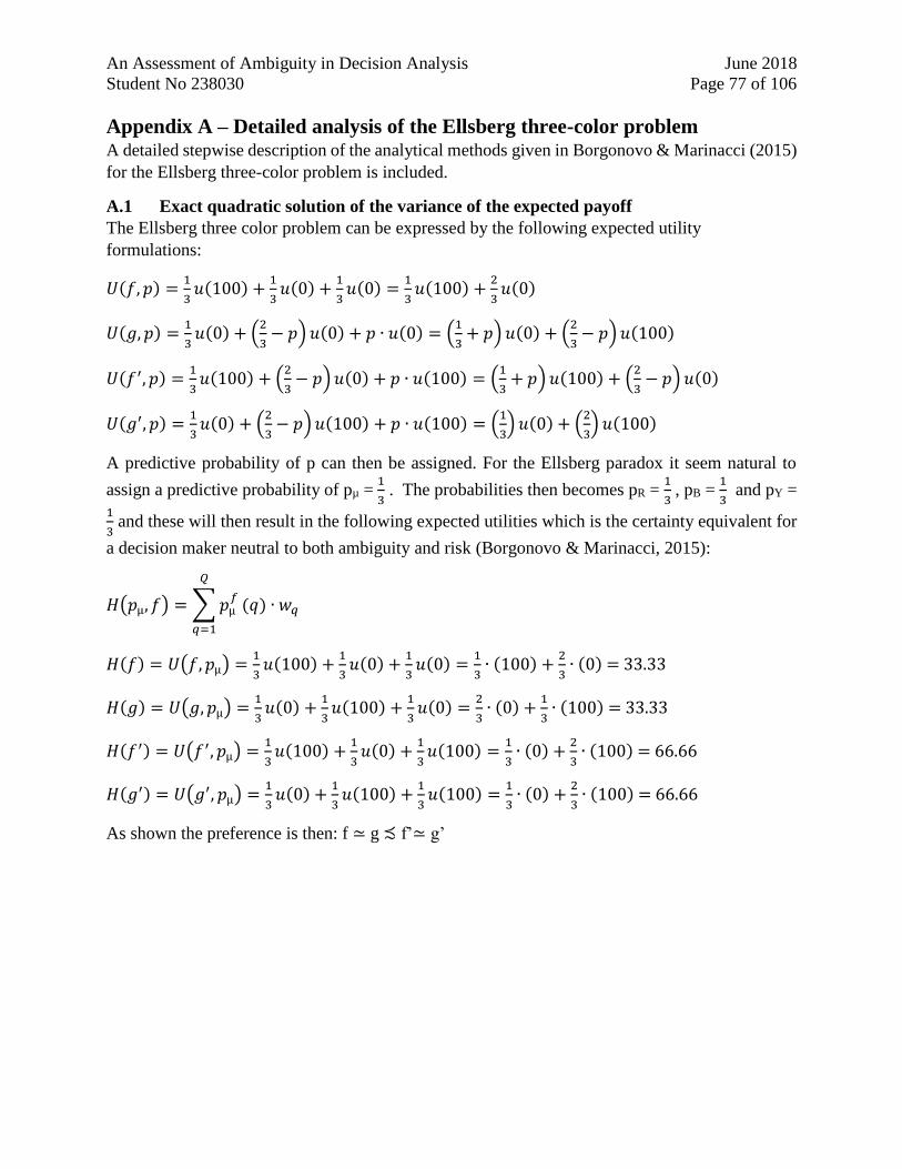
An Assessment of Ambiguity in Decision Analysis June 2018
Student No 238030 Page 77 of 106
Appendix A – Detailed analysis of the Ellsberg three-color problem A detailed stepwise description of the analytical methods given in Borgonovo & Marinacci (2015)
for the Ellsberg three-color problem is included.
A.1 Exact quadratic solution of the variance of the expected payoff
The Ellsberg three color problem can be expressed by the following expected utility
formulations:
𝑈(𝑓, 𝑝) =1
3𝑢(100) +
1
3𝑢(0) +
1
3𝑢(0) =
1
3𝑢(100) +
2
3𝑢(0)
𝑈(𝑔, 𝑝) =1
3𝑢(0) + (
2
3− 𝑝) 𝑢(0) + 𝑝 ∙ 𝑢(0) = (
1
3+ 𝑝) 𝑢(0) + (
2
3− 𝑝) 𝑢(100)
𝑈(𝑓′, 𝑝) =1
3𝑢(100) + (
2
3− 𝑝) 𝑢(0) + 𝑝 ∙ 𝑢(100) = (
1
3+ 𝑝) 𝑢(100) + (
2
3− 𝑝) 𝑢(0)
𝑈(𝑔′, 𝑝) =1
3𝑢(0) + (
2
3− 𝑝) 𝑢(100) + 𝑝 ∙ 𝑢(100) = (
1
3) 𝑢(0) + (
2
3) 𝑢(100)
A predictive probability of p can then be assigned. For the Ellsberg paradox it seem natural to
assign a predictive probability of pµ = 1
3 . The probabilities then becomes pR =
1
3 , pB =
1
3 and pY =
1
3 and these will then result in the following expected utilities which is the certainty equivalent for
a decision maker neutral to both ambiguity and risk (Borgonovo & Marinacci, 2015):
𝐻(𝑝µ, 𝑓) = ∑ 𝑝µ𝑓
𝑄
𝑞=1
(𝑞) ∙ 𝑤𝑞
𝐻(𝑓) = 𝑈(𝑓, 𝑝µ) =1
3𝑢(100) +
1
3𝑢(0) +
1
3𝑢(0) =
1
3∙ (100) +
2
3∙ (0) = 33.33
𝐻(𝑔) = 𝑈(𝑔, 𝑝µ) =1
3𝑢(0) +
1
3𝑢(100) +
1
3𝑢(0) =
2
3∙ (0) +
1
3∙ (100) = 33.33
𝐻(𝑓′) = 𝑈(𝑓′, 𝑝µ) =1
3𝑢(100) +
1
3𝑢(0) +
1
3𝑢(100) =
1
3∙ (0) +
2
3∙ (100) = 66.66
𝐻(𝑔′) = 𝑈(𝑔′, 𝑝µ) =1
3𝑢(0) +
1
3𝑢(100) +
1
3𝑢(100) =
1
3∙ (0) +
2
3∙ (100) = 66.66
As shown the preference is then: f ≃ g ≾ f’≃ g’
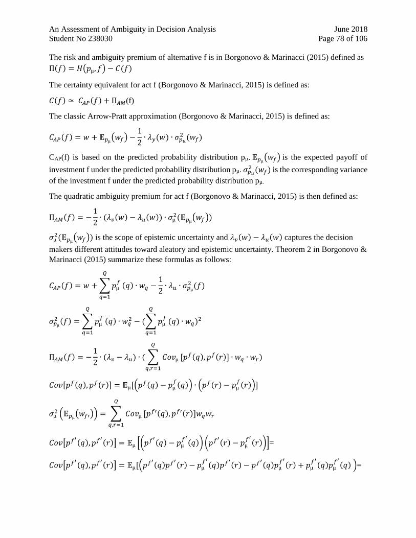
An Assessment of Ambiguity in Decision Analysis June 2018
Student No 238030 Page 78 of 106
The risk and ambiguity premium of alternative f is in Borgonovo & Marinacci (2015) defined as
П(𝑓) = 𝐻(𝑝µ, 𝑓) − 𝐶(𝑓)
The certainty equivalent for act f (Borgonovo & Marinacci, 2015) is defined as:
𝐶(𝑓) ≃ 𝐶𝐴𝑃(𝑓) + П𝐴𝑀(f)
The classic Arrow-Pratt approximation (Borgonovo & Marinacci, 2015) is defined as:
𝐶𝐴𝑃(𝑓) = 𝑤 + 𝔼𝑝µ(𝑤𝑓) −
1
2∙ 𝜆𝑦(𝑤) ∙ 𝜎𝑝𝑢
2 (𝑤𝑓)
CAP(f) is based on the predicted probability distribution pµ. 𝔼𝑝µ(𝑤𝑓) is the expected payoff of
investment f under the predicted probability distribution pµ. 𝜎𝑝𝑢2 (𝑤𝑓) is the corresponding variance
of the investment f under the predicted probability distribution pµ.
The quadratic ambiguity premium for act f (Borgonovo & Marinacci, 2015) is then defined as:
П𝐴𝑀(𝑓) = −1
2∙ (𝜆𝑣(𝑤) − 𝜆𝑢(𝑤)) ∙ 𝜎µ
2(𝔼𝑝µ(𝑤𝑓))
𝜎µ2(𝔼𝑝µ
(𝑤𝑓)) is the scope of epistemic uncertainty and 𝜆𝑣(𝑤) − 𝜆𝑢(𝑤) captures the decision
makers different attitudes toward aleatory and epistemic uncertainty. Theorem 2 in Borgonovo &
Marinacci (2015) summarize these formulas as follows:
𝐶𝐴𝑃(𝑓) = 𝑤 + ∑ 𝑝µ𝑓
𝑄
𝑞=1
(𝑞) ∙ 𝑤𝑞 −1
2∙ 𝜆𝑢 ∙ 𝜎𝑝µ
2 (𝑓)
𝜎𝑝µ2 (𝑓) = ∑ 𝑝µ
𝑓
𝑄
𝑞=1
(𝑞) ∙ 𝑤𝑞2 − (∑ 𝑝µ
𝑓
𝑄
𝑞=1
(𝑞) ∙ 𝑤𝑞)2
П𝐴𝑀(𝑓) = −1
2∙ (𝜆𝑣 − 𝜆𝑢) ∙ ( ∑ 𝐶𝑜𝑣µ
𝑄
𝑞,𝑟=1
[𝑝𝑓(𝑞), 𝑝𝑓(𝑟)] ∙ 𝑤𝑞 ∙ 𝑤𝑟)
𝐶𝑜𝑣[𝑝𝑓(𝑞), 𝑝𝑓(𝑟)] = 𝔼µ[(𝑝𝑓(𝑞) − 𝑝µ𝑓(𝑞)) ∙ (𝑝𝑓(𝑟) − 𝑝µ
𝑓(𝑟))]
𝜎µ2 (𝔼𝑝µ
(𝑤𝑓′)) = ∑ 𝐶𝑜𝑣µ
𝑄
𝑞,𝑟=1
[𝑝𝑓′(𝑞), 𝑝𝑓′(𝑟)]𝑤𝑞𝑤𝑟
𝐶𝑜𝑣[𝑝𝑓′(𝑞), 𝑝𝑓′
(𝑟)] = 𝔼µ [(𝑝𝑓′(𝑞) − 𝑝µ
𝑓′
(𝑞)) (𝑝𝑓′(𝑟) − 𝑝µ
𝑓′
(𝑟))]=
𝐶𝑜𝑣[𝑝𝑓′(𝑞), 𝑝𝑓′
(𝑟)] = 𝔼µ[(𝑝𝑓′(𝑞)𝑝𝑓′
(𝑟) − 𝑝µ𝑓′
(𝑞)𝑝𝑓′(𝑟) − 𝑝𝑓′
(𝑞)𝑝µ𝑓′
(𝑟) + 𝑝µ𝑓′
(𝑞)𝑝µ𝑓′
(𝑞) )=
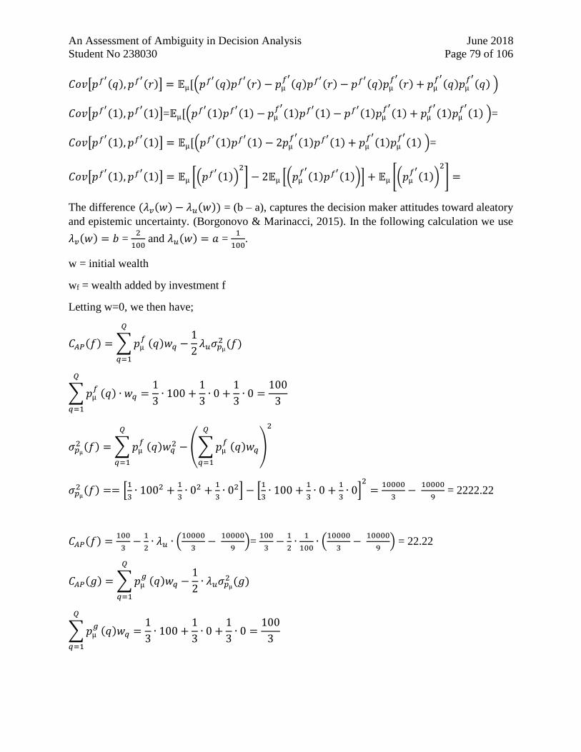
An Assessment of Ambiguity in Decision Analysis June 2018
Student No 238030 Page 79 of 106
𝐶𝑜𝑣[𝑝𝑓′(𝑞), 𝑝𝑓′
(𝑟)] = 𝔼µ[(𝑝𝑓′(𝑞)𝑝𝑓′
(𝑟) − 𝑝µ𝑓′
(𝑞)𝑝𝑓′(𝑟) − 𝑝𝑓′
(𝑞)𝑝µ𝑓′
(𝑟) + 𝑝µ𝑓′
(𝑞)𝑝µ𝑓′
(𝑞) )
𝐶𝑜𝑣[𝑝𝑓′(1), 𝑝𝑓′
(1)]=𝔼µ[(𝑝𝑓′(1)𝑝𝑓′
(1) − 𝑝µ𝑓′
(1)𝑝𝑓′(1) − 𝑝𝑓′
(1)𝑝µ𝑓′
(1) + 𝑝µ𝑓′
(1)𝑝µ𝑓′
(1) )=
𝐶𝑜𝑣[𝑝𝑓′(1), 𝑝𝑓′
(1)] = 𝔼µ[(𝑝𝑓′(1)𝑝𝑓′
(1) − 2𝑝µ𝑓′
(1)𝑝𝑓′(1) + 𝑝µ
𝑓′
(1)𝑝µ𝑓′
(1) )=
𝐶𝑜𝑣[𝑝𝑓′(1), 𝑝𝑓′
(1)] = 𝔼µ [(𝑝𝑓′(1))
2
] − 2𝔼µ [(𝑝µ𝑓′
(1)𝑝𝑓′(1))] + 𝔼µ [(𝑝µ
𝑓′
(1))2
] =
The difference (𝜆𝑣(𝑤) − 𝜆𝑢(𝑤)) = (b – a), captures the decision maker attitudes toward aleatory
and epistemic uncertainty. (Borgonovo & Marinacci, 2015). In the following calculation we use
𝜆𝑣(𝑤) = 𝑏 = 2
100 and 𝜆𝑢(𝑤) = 𝑎 =
1
100.
w = initial wealth
wf = wealth added by investment f
Letting w=0, we then have;
𝐶𝐴𝑃(𝑓) = ∑ 𝑝µ𝑓
𝑄
𝑞=1
(𝑞)𝑤𝑞 −1
2𝜆𝑢𝜎𝑝µ
2 (𝑓)
∑ 𝑝µ𝑓
𝑄
𝑞=1
(𝑞) ∙ 𝑤𝑞 =1
3∙ 100 +
1
3∙ 0 +
1
3∙ 0 =
100
3
𝜎𝑝µ2 (𝑓) = ∑ 𝑝µ
𝑓
𝑄
𝑞=1
(𝑞)𝑤𝑞2 − (∑ 𝑝µ
𝑓
𝑄
𝑞=1
(𝑞)𝑤𝑞)
2
𝜎𝑝µ2 (𝑓) == [
1
3∙ 1002 +
1
3∙ 02 +
1
3∙ 02] − [
1
3∙ 100 +
1
3∙ 0 +
1
3∙ 0]
2
=10000
3−
10000
9 = 2222.22
𝐶𝐴𝑃(𝑓) =100
3−
1
2∙ 𝜆𝑢 ∙ (
10000
3−
10000
9)=
100
3−
1
2∙
1
100∙ (
10000
3−
10000
9) = 22.22
𝐶𝐴𝑃(𝑔) = ∑ 𝑝µ𝑔
𝑄
𝑞=1
(𝑞)𝑤𝑞 −1
2∙ 𝜆𝑢𝜎𝑝µ
2 (𝑔)
∑ 𝑝µ𝑔
𝑄
𝑞=1
(𝑞)𝑤𝑞 =1
3∙ 100 +
1
3∙ 0 +
1
3∙ 0 =
100
3
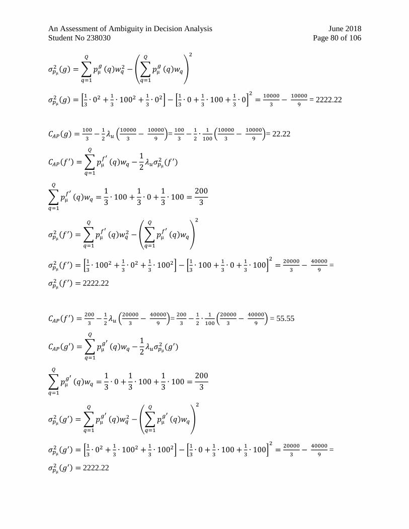
An Assessment of Ambiguity in Decision Analysis June 2018
Student No 238030 Page 80 of 106
𝜎𝑝µ2 (𝑔) = ∑ 𝑝µ
𝑔
𝑄
𝑞=1
(𝑞)𝑤𝑞2 − (∑ 𝑝µ
𝑔
𝑄
𝑞=1
(𝑞)𝑤𝑞)
2
𝜎𝑝µ2 (𝑔) = [
1
3∙ 02 +
1
3∙ 1002 +
1
3∙ 02] − [
1
3∙ 0 +
1
3∙ 100 +
1
3∙ 0]
2
=10000
3−
10000
9 = 2222.22
𝐶𝐴𝑃(𝑔) =100
3−
1
2𝜆𝑢 (
10000
3−
10000
9)=
100
3−
1
2∙
1
100(
10000
3−
10000
9)= 22.22
𝐶𝐴𝑃(𝑓′) = ∑ 𝑝µ𝑓′
𝑄
𝑞=1
(𝑞)𝑤𝑞 −1
2𝜆𝑢𝜎𝑝µ
2 (𝑓′)
∑ 𝑝µ𝑓′
𝑄
𝑞=1
(𝑞)𝑤𝑞 =1
3∙ 100 +
1
3∙ 0 +
1
3∙ 100 =
200
3
𝜎𝑝µ2 (𝑓′) = ∑ 𝑝µ
𝑓′
𝑄
𝑞=1
(𝑞)𝑤𝑞2 − (∑ 𝑝µ
𝑓′
𝑄
𝑞=1
(𝑞)𝑤𝑞)
2
𝜎𝑝µ2 (𝑓′) = [
1
3∙ 1002 +
1
3∙ 02 +
1
3∙ 1002] − [
1
3∙ 100 +
1
3∙ 0 +
1
3∙ 100]
2
=20000
3−
40000
9 =
𝜎𝑝µ2 (𝑓′) = 2222.22
𝐶𝐴𝑃(𝑓′) =200
3−
1
2𝜆𝑢 (
20000
3−
40000
9)=
200
3−
1
2∙
1
100(
20000
3−
40000
9) = 55.55
𝐶𝐴𝑃(𝑔′) = ∑ 𝑝µ𝑔′
𝑄
𝑞=1
(𝑞)𝑤𝑞 −1
2𝜆𝑢𝜎𝑝µ
2 (𝑔′)
∑ 𝑝µ𝑔′
𝑄
𝑞=1
(𝑞)𝑤𝑞 =1
3∙ 0 +
1
3∙ 100 +
1
3∙ 100 =
200
3
𝜎𝑝µ2 (𝑔′) = ∑ 𝑝µ
𝑔′
𝑄
𝑞=1
(𝑞)𝑤𝑞2 − (∑ 𝑝µ
𝑔′
𝑄
𝑞=1
(𝑞)𝑤𝑞)
2
𝜎𝑝µ2 (𝑔′) = [
1
3∙ 02 +
1
3∙ 1002 +
1
3∙ 1002] − [
1
3∙ 0 +
1
3∙ 100 +
1
3∙ 100]
2
=20000
3−
40000
9 =
𝜎𝑝µ2 (𝑔′) = 2222.22
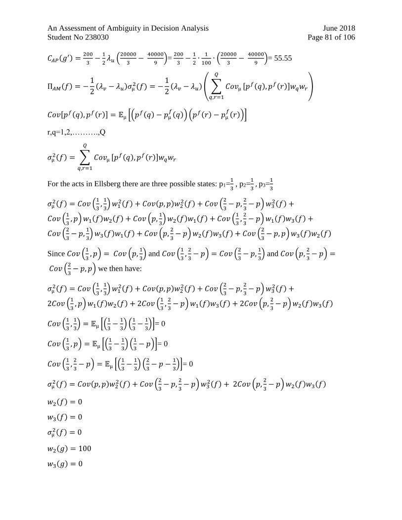
An Assessment of Ambiguity in Decision Analysis June 2018
Student No 238030 Page 81 of 106
𝐶𝐴𝑃(𝑔′) =200
3−
1
2𝜆𝑢 (
20000
3−
40000
9)=
200
3−
1
2∙
1
100∙ (
20000
3−
40000
9)= 55.55
П𝐴𝑀(𝑓) = −1
2(𝜆𝑣 − 𝜆𝑢)𝜎µ
2(𝑓) = −1
2(𝜆𝑣 − 𝜆𝑢) ( ∑ 𝐶𝑜𝑣µ
𝑄
𝑞,𝑟=1
[𝑝𝑓(𝑞), 𝑝𝑓(𝑟)]𝑤𝑞𝑤𝑟)
𝐶𝑜𝑣[𝑝𝑓(𝑞), 𝑝𝑓(𝑟)] = 𝔼µ [(𝑝𝑓(𝑞) − 𝑝µ𝑓(𝑞)) (𝑝𝑓(𝑟) − 𝑝µ
𝑓(𝑟))]
r,q=1,2,……….,Q
𝜎µ2(𝑓) = ∑ 𝐶𝑜𝑣µ
𝑄
𝑞,𝑟=1
[𝑝𝑓(𝑞), 𝑝𝑓(𝑟)]𝑤𝑞𝑤𝑟
For the acts in Ellsberg there are three possible states: p1=1
3 , p2=
1
3 , p3=
1
3
𝜎µ2(𝑓) = 𝐶𝑜𝑣 (
1
3,
1
3) 𝑤1
2(𝑓) + 𝐶𝑜𝑣(𝑝, 𝑝)𝑤22(𝑓) + 𝐶𝑜𝑣 (
2
3− 𝑝,
2
3− 𝑝) 𝑤3
2(𝑓) +
𝐶𝑜𝑣 (1
3, 𝑝) 𝑤1(𝑓)𝑤2(𝑓) + 𝐶𝑜𝑣 (𝑝,
1
3) 𝑤2(𝑓)𝑤1(𝑓) + 𝐶𝑜𝑣 (
1
3,
2
3− 𝑝) 𝑤1(𝑓)𝑤3(𝑓) +
𝐶𝑜𝑣 (2
3− 𝑝,
1
3) 𝑤3(𝑓)𝑤1(𝑓) + 𝐶𝑜𝑣 (𝑝,
2
3− 𝑝) 𝑤2(𝑓)𝑤3(𝑓) + 𝐶𝑜𝑣 (
2
3− 𝑝, 𝑝) 𝑤3(𝑓)𝑤2(𝑓)
Since 𝐶𝑜𝑣 (1
3, 𝑝) = 𝐶𝑜𝑣 (𝑝,
1
3) and 𝐶𝑜𝑣 (
1
3,
2
3− 𝑝) = 𝐶𝑜𝑣 (
2
3− 𝑝,
1
3) and 𝐶𝑜𝑣 (𝑝,
2
3− 𝑝) =
𝐶𝑜𝑣 (2
3− 𝑝, 𝑝) we then have:
𝜎µ2(𝑓) = 𝐶𝑜𝑣 (
1
3,
1
3) 𝑤1
2(𝑓) + 𝐶𝑜𝑣(𝑝, 𝑝)𝑤22(𝑓) + 𝐶𝑜𝑣 (
2
3− 𝑝,
2
3− 𝑝) 𝑤3
2(𝑓) +
2𝐶𝑜𝑣 (1
3, 𝑝) 𝑤1(𝑓)𝑤2(𝑓) + 2𝐶𝑜𝑣 (
1
3,
2
3− 𝑝) 𝑤1(𝑓)𝑤3(𝑓) + 2𝐶𝑜𝑣 (𝑝,
2
3− 𝑝) 𝑤2(𝑓)𝑤3(𝑓)
𝐶𝑜𝑣 (1
3,
1
3) = 𝔼µ [(
1
3−
1
3) (
1
3−
1
3)]= 0
𝐶𝑜𝑣 (1
3, 𝑝) = 𝔼µ [(
1
3−
1
3) (
1
3− 𝑝)]= 0
𝐶𝑜𝑣 (1
3,
2
3− 𝑝) = 𝔼µ [(
1
3−
1
3) (
2
3− 𝑝 −
1
3)]= 0
𝜎µ2(𝑓) = 𝐶𝑜𝑣(𝑝, 𝑝)𝑤2
2(𝑓) + 𝐶𝑜𝑣 (2
3− 𝑝,
2
3− 𝑝) 𝑤3
2(𝑓) + 2𝐶𝑜𝑣 (𝑝,2
3− 𝑝) 𝑤2(𝑓)𝑤3(𝑓)
𝑤2(𝑓) = 0
𝑤3(𝑓) = 0
𝜎µ2(𝑓) = 0
𝑤2(𝑔) = 100
𝑤3(𝑔) = 0
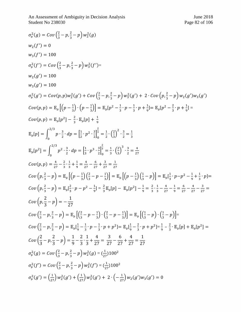
An Assessment of Ambiguity in Decision Analysis June 2018
Student No 238030 Page 82 of 106
𝜎µ2(𝑔) = 𝐶𝑜𝑣 (
2
3− 𝑝,
2
3− 𝑝) 𝑤2
2(𝑔)
𝑤2(𝑓′) = 0
𝑤3(𝑓′) = 100
𝜎µ2(𝑓′) = 𝐶𝑜𝑣 (
2
3− 𝑝,
2
3− 𝑝) 𝑤3
2(𝑓′)=
𝑤2(𝑔′) = 100
𝑤3(𝑔′) = 100
𝜎µ2(𝑔′) = 𝐶𝑜𝑣(𝑝, 𝑝)𝑤2
2(𝑔′) + 𝐶𝑜𝑣 (2
3− 𝑝,
2
3− 𝑝) 𝑤3
2(𝑔′) + 2 ∙ 𝐶𝑜𝑣 (𝑝,2
3− 𝑝) 𝑤2(𝑔′)𝑤3(𝑔′)
𝐶𝑜𝑣(𝑝, 𝑝) = 𝔼µ [(𝑝 −1
3) ∙ (𝑝 −
1
3)] = 𝔼µ[𝑝2 −
1
3∙ 𝑝 −
1
3∙ 𝑝 +
1
9]= 𝔼µ[𝑝2 −
2
3∙ 𝑝 +
1
9] =
𝐶𝑜𝑣(𝑝, 𝑝) = 𝔼µ[𝑝2] − 2
3∙ 𝔼µ[𝑝] +
1
9
𝔼µ[𝑝] = ∫ 𝑝 ∙3
2
2/3
0
∙ 𝑑𝑝 = [1
2∙ 𝑝2 ∙
3
2]
0
2
3=
1
2∙ (
2
3)
2
∙3
2=
1
3
𝔼µ[𝑝2] = ∫ 𝑝2 ∙3
2
2/3
0
∙ 𝑑𝑝 = [1
3∙ 𝑝3 ∙
3
2]
0
2
3=
1
3∙ (
2
3)
3
∙3
2=
4
27
𝐶𝑜𝑣(𝑝, 𝑝) =4
27−
2
3∙
1
3+
1
9=
4
27−
6
27+
3
27=
1
27
𝐶𝑜𝑣 (𝑝,2
3− 𝑝) = 𝔼µ [(𝑝 −
1
3) (
2
3− 𝑝 −
1
3)] = 𝔼µ [(𝑝 −
1
3) (
1
3− 𝑝)] = 𝔼µ[
1
3∙ 𝑝−𝑝2 −
1
9+
1
3∙ 𝑝]=
𝐶𝑜𝑣 (𝑝,2
3− 𝑝) = 𝔼µ[
2
3∙ 𝑝 − 𝑝2 −
1
9] =
2
3𝔼µ[𝑝] − 𝔼µ[𝑝2] −
1
9=
2
3∙
1
3−
4
27−
1
9=
6
27−
4
27−
3
27=
𝐶𝑜𝑣 (𝑝,2
3− 𝑝) = −
1
27
𝐶𝑜𝑣 (2
3− 𝑝,
2
3− 𝑝) = 𝔼µ [(
2
3− 𝑝 −
1
3) ∙ (
2
3− 𝑝 −
1
3)] = 𝔼µ [(
1
3− 𝑝) ∙ (
1
3− 𝑝)]=
𝐶𝑜𝑣 (2
3− 𝑝,
2
3− 𝑝) = 𝔼µ[
1
9−
1
3∙ 𝑝 −
1
3∙ 𝑝 + 𝑝2]= 𝔼µ[
1
9−
2
3∙ 𝑝 + 𝑝2]=
1
9 –
2
3∙ 𝔼µ[𝑝] + 𝔼µ[𝑝2] =
𝐶𝑜𝑣 (2
3− 𝑝,
2
3− 𝑝) =
1
9−
2
3∙
1
3+
4
27=
3
27−
6
27+
4
27=
1
27
𝜎µ2(𝑔) = 𝐶𝑜𝑣 (
2
3− 𝑝,
2
3− 𝑝) 𝑤2
2(𝑔) = (1
27)1002
𝜎µ2(𝑓′) = 𝐶𝑜𝑣 (
2
3− 𝑝,
2
3− 𝑝) 𝑤3
2(𝑓′) = (1
27)1002
𝜎µ2(𝑔′) = (
1
27) 𝑤2
2(𝑔′) + (1
27) 𝑤3
2(𝑔′) + 2 ∙ (−1
27) 𝑤2(𝑔′)𝑤3(𝑔′) = 0
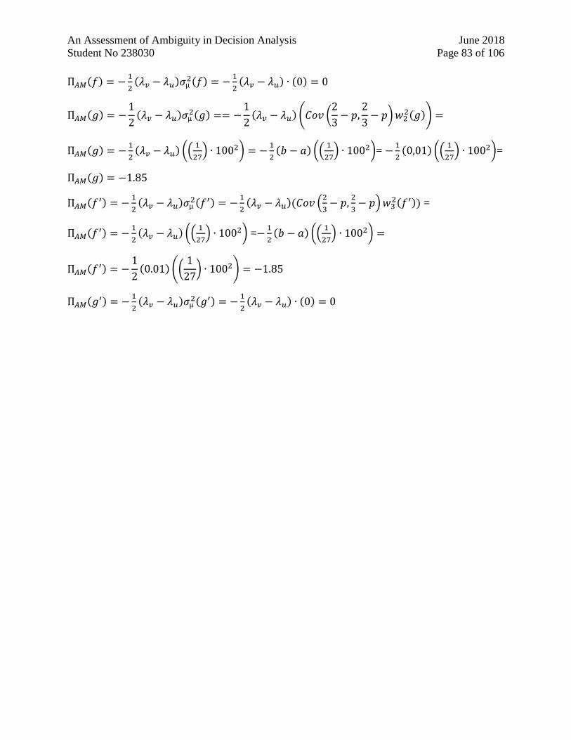
An Assessment of Ambiguity in Decision Analysis June 2018
Student No 238030 Page 83 of 106
П𝐴𝑀(𝑓) = −1
2(𝜆𝑣 − 𝜆𝑢)𝜎µ
2(𝑓) = −1
2(𝜆𝑣 − 𝜆𝑢) ∙ (0) = 0
П𝐴𝑀(𝑔) = −1
2(𝜆𝑣 − 𝜆𝑢)𝜎µ
2(𝑔) == −1
2(𝜆𝑣 − 𝜆𝑢) (𝐶𝑜𝑣 (
2
3− 𝑝,
2
3− 𝑝) 𝑤2
2(𝑔)) =
П𝐴𝑀(𝑔) = −1
2(𝜆𝑣 − 𝜆𝑢) ((
1
27) ∙ 1002) = −
1
2(𝑏 − 𝑎) ((
1
27) ∙ 1002)= −
1
2(0,01) ((
1
27) ∙ 1002)=
П𝐴𝑀(𝑔) = −1.85
П𝐴𝑀(𝑓′) = −1
2(𝜆𝑣 − 𝜆𝑢)𝜎µ
2(𝑓′) = −1
2(𝜆𝑣 − 𝜆𝑢)(𝐶𝑜𝑣 (
2
3− 𝑝,
2
3− 𝑝) 𝑤3
2(𝑓′)) =
П𝐴𝑀(𝑓′) = −1
2(𝜆𝑣 − 𝜆𝑢) ((
1
27) ∙ 1002) =−
1
2(𝑏 − 𝑎) ((
1
27) ∙ 1002) =
П𝐴𝑀(𝑓′) = −1
2(0.01) ((
1
27) ∙ 1002) = −1.85
П𝐴𝑀(𝑔′) = −1
2(𝜆𝑣 − 𝜆𝑢)𝜎µ
2(𝑔′) = −1
2(𝜆𝑣 − 𝜆𝑢) ∙ (0) = 0
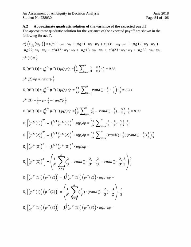
An Assessment of Ambiguity in Decision Analysis June 2018
Student No 238030 Page 84 of 106
A.2 Approximate quadratic solution of the variance of the expected payoff
The approximate quadratic solution for the variance of the expected payoff are shown in the
following for act f’.
𝜎µ2 (𝔼𝑝µ
(𝑤𝑓′)) =𝑠𝑖𝑔11 ∙ 𝑤1 ∙ 𝑤1 + 𝑠𝑖𝑔21 ∙ 𝑤2 ∙ 𝑤1 + 𝑠𝑖𝑔31 ∙ 𝑤3 ∙ 𝑤1 + 𝑠𝑖𝑔12 ∙ 𝑤1 ∙ 𝑤2 +
𝑠𝑖𝑔22 ∙ 𝑤2 ∙ 𝑤2 + 𝑠𝑖𝑔32 ∙ 𝑤3 ∙ 𝑤2 + 𝑠𝑖𝑔13 ∙ 𝑤1 ∙ 𝑤3 + 𝑠𝑖𝑔23 ∙ 𝑤2 ∙ 𝑤3 + 𝑠𝑖𝑔33 ∙ 𝑤3 ∙ 𝑤3
𝑝𝑓′(1)= 1
3
𝔼µ[𝑝𝑓′(1)]= ∫ 𝑝𝑓′(1)2/3
0µ(p)dp =(
1
𝑁 ∑
1
3
𝑁
𝑁=1 ∙
3
2 ) ∙
2
3 = 0.33
𝑝𝑓′(2)=p = rand()∙ 2
3
𝔼µ[𝑝𝑓′(2)]= ∫ 𝑝𝑓′(2)2/3
0µ(p) dp = (
1
𝑁 ∑ 𝑟𝑎𝑛𝑑() ∙
2
3
𝑁
𝑁=1 ∙
3
2 ) ∙
2
3 = 0.33
𝑝𝑓′(3) = 2
3 – p=
2
3− rand()∙
2
3
𝔼µ[𝑝𝑓′(3)]= ∫ 𝑝𝑓′(3)2/3
0 µ(p)dp =(
1
𝑁 ∑ (
2
3− 𝑟𝑎𝑛𝑑() ∙
2
3)
𝑁
𝑁=1 ∙
3
2 ) ∙
2
3 = 0.33
𝔼µ [(𝑝𝑓′(1))2
] = ∫ (𝑝𝑓′(1))2
∙2/3
0 µ(p)dp = (
1
𝑁 ∑ (
1
3
𝑁
𝑁=1 ∙
1
3) ∙
3
2 ) ∙
2
3
𝔼µ [(𝑝𝑓′(2))2
] = ∫ (𝑝𝑓′(2))2
∙2/3
0 µ(p)dp = (
1
𝑁 ∑ (𝑟𝑎𝑛𝑑() ∙
2
3
𝑁
𝑁=1 )(𝑟𝑎𝑛𝑑() ∙
2
3 )
3
2 )
2
3
𝔼µ [(𝑝𝑓′(3))2
] = ∫ (𝑝𝑓′(3))2
∙2/3
0 µ(p)dp =
𝔼µ [(𝑝𝑓′(3))2
] = (1
𝑁 ∑(
2
3− 𝑟𝑎𝑛𝑑() ∙
2
3)
𝑁
𝑁=1
∙ (2
3− 𝑟𝑎𝑛𝑑() ∙
2
3)
3
2 )
2
3
𝔼µ [(𝑝𝑓′(1)) (𝑝𝑓′
(2))] = ∫ (𝑝𝑓′(1)) (𝑝𝑓′
(2)) ∙2
30
µ(p)∙ dp =
𝔼µ [(𝑝𝑓′(1)) (𝑝𝑓′
(2))] = (1
𝑁 ∑(
1
3
𝑁
𝑁=1
) ∙ (𝑟𝑎𝑛𝑑() ∙ 2
3 ) ∙
3
2 ) ∙
2
3
𝔼µ [(𝑝𝑓′(1)) (𝑝𝑓′
(3))] = ∫ (𝑝𝑓′(1)) (𝑝𝑓′
(3)) ∙2
30
µ(p)∙ dp =
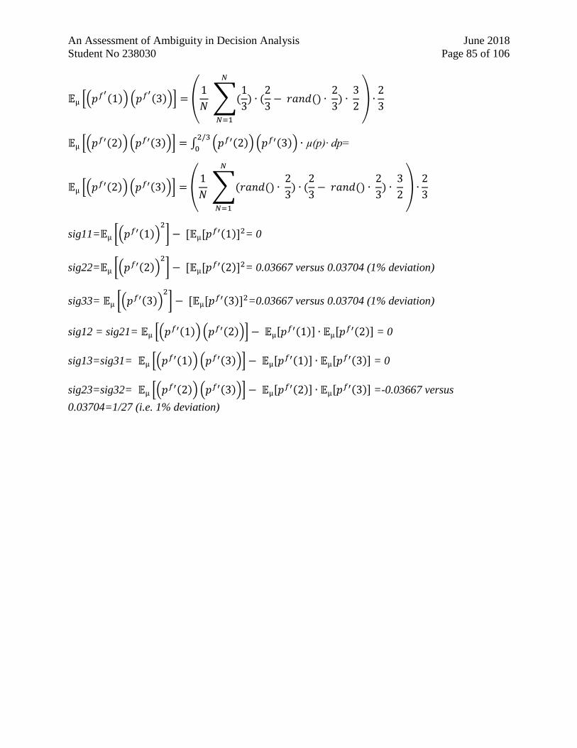
An Assessment of Ambiguity in Decision Analysis June 2018
Student No 238030 Page 85 of 106
𝔼µ [(𝑝𝑓′(1)) (𝑝𝑓′
(3))] = (1
𝑁 ∑(
1
3)
𝑁
𝑁=1
∙ (2
3− 𝑟𝑎𝑛𝑑() ∙
2
3) ∙
3
2 ) ∙
2
3
𝔼µ [(𝑝𝑓′(2)) (𝑝𝑓′(3))] = ∫ (𝑝𝑓′(2)) (𝑝𝑓′(3)) ∙2/3
0 µ(p)∙ dp=
𝔼µ [(𝑝𝑓′(2)) (𝑝𝑓′(3))] = (1
𝑁 ∑(𝑟𝑎𝑛𝑑() ∙
2
3)
𝑁
𝑁=1
∙ (2
3− 𝑟𝑎𝑛𝑑() ∙
2
3) ∙
3
2 ) ∙
2
3
sig11=𝔼µ [(𝑝𝑓′(1))2
] − [𝔼µ[𝑝𝑓′(1)]2= 0
sig22=𝔼µ [(𝑝𝑓′(2))2
] − [𝔼µ[𝑝𝑓′(2)]2= 0.03667 versus 0.03704 (1% deviation)
sig33= 𝔼µ [(𝑝𝑓′(3))2
] − [𝔼µ[𝑝𝑓′(3)]2=0.03667 versus 0.03704 (1% deviation)
sig12 = sig21= 𝔼µ [(𝑝𝑓′(1)) (𝑝𝑓′(2))] − 𝔼µ[𝑝𝑓′(1)] ∙ 𝔼µ[𝑝𝑓′(2)] = 0
sig13=sig31= 𝔼µ [(𝑝𝑓′(1)) (𝑝𝑓′(3))] − 𝔼µ[𝑝𝑓′(1)] ∙ 𝔼µ[𝑝𝑓′(3)] = 0
sig23=sig32= 𝔼µ [(𝑝𝑓′(2)) (𝑝𝑓′(3))] − 𝔼µ[𝑝𝑓′(2)] ∙ 𝔼µ[𝑝𝑓′(3)] =-0.03667 versus
0.03704=1/27 (i.e. 1% deviation)
An Assessment of Ambiguity in Decision Analysis June 2018
Student No 238030 Page 86 of 106
A.3 Solving the smooth ambiguity functional
The smooth ambiguity aversion (Klibanoff, et al., 2005) is described as an increasing concave
function of the subjective utility function.
𝑉(𝑓) = ∫ 𝑣(𝑐(𝑓, 𝑝)) ∙ 𝑑µ(𝑝)
𝛥(𝑆)
= ∫ 𝑣(𝑢−1(𝑢(𝑓, 𝑝))) ∙ 𝑑µ(𝑝)
𝛥(𝑆)
𝑉(𝑔) = ∫ 𝑣(𝑐(𝑔, 𝑝)) ∙ 𝑑µ(𝑝)
𝛥(𝑆)
= ∫ 𝑣(𝑢−1(𝑢(𝑔, 𝑝))) ∙ 𝑑µ(𝑝)
𝛥(𝑆)
𝑉(𝑓′) = ∫ 𝑣(𝑐(𝑓′, 𝑝)) ∙ 𝑑µ(𝑝)
𝛥(𝑆)
= ∫ 𝑣(𝑢−1(𝑢(𝑓′, 𝑝))) ∙ 𝑑µ(𝑝)
𝛥(𝑆)
𝑉(𝑔′) = ∫ 𝑣(𝑐(𝑔′, 𝑝)) ∙ 𝑑µ(𝑝)
𝛥(𝑆)
= ∫ 𝑣(𝑢−1(𝑢(𝑔′, 𝑝))) ∙ 𝑑µ(𝑝)
𝛥(𝑆)
First we find the utility function for the acts that also includes risk aversion by the exponential
function and the risk aversion constant a:
𝑢(f, p) = 1
3𝑢(100) +
2
3𝑢(0) =
1
3(−e−a ∙(100)) +
2
3(−e−a ∙(0)) =
1
3(−e−a ∙(100)) +
2
3(-1) =
𝑢(f, p) = −1
3[e−a ∙(100) + 2]
𝑢(g, p) = (1
3+ 𝑝)𝑢(0) + (
2
3− 𝑝)𝑢(100) = (
1
3+ 𝑝)(−e−a ∙(0)) + (
2
3− 𝑝)(−e−a ∙(100)) =
𝑢(g, p) = −[1
3+ 𝑝 + (
2
3− 𝑝)e−a ∙(100)]
𝑢(f ′, p) = (1 − 𝑝)𝑢(100) + 𝑝 ∙ 𝑢(0) = (1 − 𝑝)(−e−a ∙(100)) + 𝑝(−e−a ∙(0)) =
𝑢(f ′, p) = −[(1 − 𝑝)e−a ∙(100) + 𝑝]
𝑢(g′, p) =1
3𝑢(0) +
2
3𝑢(100) =
1
3(−e−a ∙(0)) +
2
3(−e−a ∙(100)) = −[
1
3+
2
3e−a ∙(100)]
The certainty equivalent function of the subjective expected utility function is then found as the
inverse of the utility function:
𝑐(𝑓, 𝑝) = 𝑢−1(𝑢(𝑓, 𝑝)) = - 1
𝑎ln(−𝑢(𝑓, 𝑝)) = -
1
𝑎ln [
1
3(e−a ∙(100) + 2)]
𝑐(𝑔, 𝑝) = 𝑢−1(𝑢(𝑔, 𝑝)) = - 1
𝑎ln(−𝑢(𝑔, 𝑝)) = -
1
𝑎 ln[
1
3+ 𝑝 + (
2
3− 𝑝)e−a ∙(100)]
𝑐(𝑓′, 𝑝) = 𝑢−1(𝑢(𝑓′, 𝑝)) = - 1
𝑎ln(−𝑢(𝑓′, 𝑝)) = -
1
𝑎ln[(1 − 𝑝)e−a ∙(100) + 𝑝]
𝑐(𝑔′, 𝑝) = 𝑢−1(𝑢(𝑔′, 𝑝)) = - 1
𝑎ln(−𝑢(𝑓𝑔′, 𝑝)) = -
1
𝑎ln[
1
3+
2
3e−a ∙(100)]
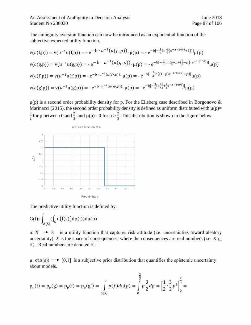
An Assessment of Ambiguity in Decision Analysis June 2018
Student No 238030 Page 87 of 106
The ambiguity aversion function can now be introduced as an exponential function of the
subjective expected utility function.
v(𝑐(f,p)) = v(𝑢−1u(f,p)) = - e−b ∙ 𝑢−1(𝑢(𝑓, 𝑝))∙ µ(p) = - e−b[− 1
𝑎 ln (
1
3(e−a ∙(100)+2))]µ(p)
v(𝑐(g,p)) = v(𝑢−1u(g,p)) = - e−b ∙ 𝑢−1(𝑢(𝑔, 𝑝))∙ µ(p) = - e−b[− 1
𝑎 ∙ln(
1
3+𝑝+(
2
3−𝑝)∙ e−a ∙(100))]µ(p)
v(𝑐(f’,p)) = v(𝑢−1u(f’,p)) = - e−b ∙ 𝑢−1(𝑢(𝑓′,𝑝))∙ µ(p) = - e−b[− 1
𝑎ln((1−𝑝)e−a ∙(100)+𝑝)]µ(p)
v(𝑐(g’,p)) = v(𝑢−1u(g’,p)) = - e−b ∙ 𝑢−1(𝑢(𝑔′,𝑝))∙ µ(p) = - e−b[− 1
𝑎ln(
1
3+
2
3e−a ∙(100))]µ(p)
µ(p) is a second order probability density for p. For the Ellsberg case described in Borgonovo &
Marinacci (2015), the second order probability density is defined as uniform distributed with µ(p)= 3
2 for p between 0 and
2
3 and µ(p)= 0 for p >
2
3. This distribution is shown in the figure below.
The predictive utility function is defined by:
G(f)=∫ (∫ u(f(s))dp(i))dµ(p)S
Δ(S)
u: X ℝ is a utility function that captures risk attitude (i.e. uncertainties toward aleatory
uncertainty). X is the space of consequences, where the consequences are real numbers (i.e. X ⸦
ℝ). Real numbers are denoted ℝ.
µ: σ(Δ(s)) [0,1] is a subjective prior distribution that quantifies the epistemic uncertainty
about models.
pµ(f) = pµ(g) = pµ(f) = pµ(g′) = ∫ 𝑝(𝑓)𝑑µ(𝑝)
𝛥(𝑆)
= ∫ 𝑝3
2𝑑𝑝
23
0
= [1
2∙
3
2𝑝2]
0
23
=
An Assessment of Ambiguity in Decision Analysis June 2018
Student No 238030 Page 88 of 106
pµ(f) = pµ(g) = pµ(f) = pµ(g′) = [3
4∙
4
9− 0] =
1
3
pµ is the predictive probability pµ ϵ Δ(S). The probabilities then becomes P(Red) = 1
3 , P(Blue) =
1
3
and P(Yellow) = 1
3 and these will then result in the following predicted subjective expected
utilities:
𝐺(𝑓) = 𝑈(𝑓, 𝑝µ) =1
3(100) +
1
3(0) +
1
3(0) =
1
3(100) +
2
3(0) = 33.33
𝐺(𝑔) = 𝑈(𝑔, 𝑝µ) =1
3(0) +
1
3(100) +
1
3(0) =
2
3(0) +
1
3(100) = 33.33
𝐺(𝑓′) = 𝑈(𝑓′, 𝑝µ) =1
3(100) +
1
3(0) +
1
3(100) =
1
3(0) +
2
3(100) = 66.66
𝐺(𝑔′) = 𝑈(𝑔′, 𝑝µ) =1
3(0) +
1
3(100) +
1
3(100) =
1
3(0) +
2
3(100) = 66.66
The total risk and ambiguity aversion is then found by integration for p ϵ (0, 2
3 ):
V(f)=∫ v(u(w))2/3
0dµp = ∫ - e−b[−
1
𝑎ln(
1
3(e−a ∙(100)+2))]∙
3
2
2/3
0
dp
V(g)=∫ v(u(w))2/3
0dµp = ∫ - e−b[−
1
𝑎ln(
1
3+𝑝+(
2
3−𝑝)e−a ∙(100))]∙
3
2
2/3
0
dp
V(f’)=∫ v(u(w))2/3
0dµp = ∫ - e−b ∙[−
1
𝑎 ∙ ln((1−𝑝)∙ e−a ∙(100)+𝑝)]∙
3
2
2/3
0
dp
V(g’)=∫ v(u(w))2/3
0dµp = ∫ - e−b[−
1
𝑎ln(
1
3+
2
3e−a ∙(100))]∙
3
2
2/3
0
dp
The above integrals are numerically estimated. The v(u(w)) function has been calculated N=5000
times by the use of the constants a = 1
100 and b=
2
100 and the probability p simulated by the Excel
function, p = rand() ∙ 2
3 .
V(f)=( 1
𝑁∑ - e−b[−
1
𝑎 ln(
1
3(e−a ∙(100)+2))]∙
3
2
𝑁
𝑁=1 )
2
3 = -0.62
V(g)=(1
𝑁∑ - e−b[−
1
𝑎 ln(
1
3+𝑟𝑎𝑛𝑑()∙
2
3 +(
2
3−𝑝)e−a ∙(100))]∙
3
2
𝑁
𝑁=1 )
2
3 = -0.64
V(f’)=(1
𝑁∑ - e−b[−
1
𝑎 ln(−
1
𝑎 ln((1−𝑟𝑎𝑛𝑑() ∙
2
3)e−a ∙(100)+𝑟𝑎𝑛𝑑() ∙
2
3))]∙
3
2
2/3
0 )
2
3 = -0.35
V(g’)=(1
𝑁∑ - e−b[−
1
𝑎 ln(−
1
𝑎 ln(
1
3+
2
3 e−a ∙(100)))]∙
3
2
2/3
0 )
2
3 = -0.33
An Assessment of Ambiguity in Decision Analysis June 2018
Student No 238030 Page 89 of 106
The certainty equivalent using the smooth ambiguity aversion have the following general
expression:
𝐶(𝑓) = 𝑣−1(𝑉(𝑓)) = 𝑣−1 [ ∫ 𝑣(𝑐(𝑓, 𝑝))𝑑µ(𝑝)
𝛥(𝑆)
] = 𝑣−1 [ ∫ 𝑣(𝑢−1(𝑢(𝑓, 𝑝)))𝑑µ(𝑝)
𝛥(𝑆)
]
𝐶(𝑓) = 𝑣−1(𝑉(𝑓)) = − 1
𝑏ln[−𝑉(𝑓)] = −
1
𝑏ln [− ∫ - e−b[−
1
𝑎 ln(
1
3 [e−a ∙(100)+2])]∙
3
2
2/3
0
dp]
𝐶(𝑔) = 𝑣−1(𝑉(𝑓)) = 𝑣−1 [ ∫ 𝑣(𝑐(𝑓, 𝑝))𝑑µ(𝑝)
𝛥(𝑆)
] = 𝑣−1 [ ∫ 𝑣(𝑢−1(𝑢(𝑓, 𝑝)))𝑑µ(𝑝)
𝛥(𝑆)
]
𝐶(𝑔) = 𝑣−1(𝑉(𝑓)) = −1
𝑏ln[−𝑉(𝑓)] =
𝐶(𝑔) = −1
𝑏ln[− ∫ - e−b[−
1
𝑎 ln(
1
3+𝑟𝑎𝑛𝑑()∙
2
3 +(
2
3−𝑝)e−a ∙(100))]∙
3
2
2/3
0
dp]
𝐶(𝑓′) = 𝑣−1(𝑉(𝑓)) = 𝑣−1 [ ∫ 𝑣(𝑐(𝑓, 𝑝))𝑑µ(𝑝)
𝛥(𝑆)
] = 𝑣−1 [ ∫ 𝑣(𝑢−1(𝑢(𝑓, 𝑝)))𝑑µ(𝑝)
𝛥(𝑆)
]
𝐶(𝑓′) = 𝑣−1(𝑉(𝑓)) = − 1
𝑏ln[−𝑉(𝑓)] =
𝐶(𝑓′) = − 1
𝑏ln [− ∫ - e−b[−
1
𝑎 ln(−
1
𝑎 ln((1−𝑟𝑎𝑛𝑑() ∙
2
3)e−a ∙(100)+𝑟𝑎𝑛𝑑() ∙
2
3))]∙
3
2
2/3
0
dp]
𝐶(𝑔′) = 𝑣−1(𝑉(𝑓)) = 𝑣−1 [ ∫ 𝑣(𝑐(𝑓, 𝑝))𝑑µ(𝑝)
𝛥(𝑆)
] = 𝑣−1 [ ∫ 𝑣(𝑢−1(𝑢(𝑓, 𝑝)))𝑑µ(𝑝)
𝛥(𝑆)
]
𝐶(𝑔′) = 𝑣−1(𝑉(𝑓)) = − 1
𝑏ln[−𝑉(𝑓)] =
𝐶(𝑔′) = − 1
𝑏ln [− ∫ - e−b[−
1
𝑎 ln(−
1
𝑎 ln(
1
3+
2
3 e−a ∙(100))]∙
3
2
2/3
0
dp]
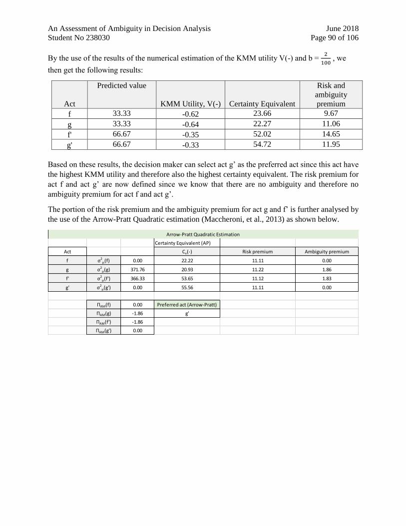
An Assessment of Ambiguity in Decision Analysis June 2018
Student No 238030 Page 90 of 106
By the use of the results of the numerical estimation of the KMM utility V(-) and b = 2
100 , we
then get the following results:
Act
Predicted value
KMM Utility, V(-) Certainty Equivalent
Risk and
ambiguity
premium
f 33.33 -0.62 23.66 9.67
g 33.33 -0.64 22.27 11.06
f' 66.67 -0.35 52.02 14.65
g' 66.67 -0.33 54.72 11.95
Based on these results, the decision maker can select act g’ as the preferred act since this act have
the highest KMM utility and therefore also the highest certainty equivalent. The risk premium for
act f and act g’ are now defined since we know that there are no ambiguity and therefore no
ambiguity premium for act f and act g’.
The portion of the risk premium and the ambiguity premium for act g and f’ is further analysed by
the use of the Arrow-Pratt Quadratic estimation (Maccheroni, et al., 2013) as shown below.
Certainty Equivalent (AP)
Act Cv(-) Risk premium Ambiguity premium
f σ2µ(f) 0.00 22.22 11.11 0.00
g σ2µ(g) 371.76 20.93 11.22 1.86
f' σ2µ(f') 366.33 53.65 11.12 1.83
g' σ2µ(g') 0.00 55.56 11.11 0.00
ПAM(f) 0.00 Preferred act (Arrow-Pratt)
ПAM(g) -1.86 g'
ПAM(f') -1.86
ПAM(g') 0.00
Arrow-Pratt Quadratic Estimation
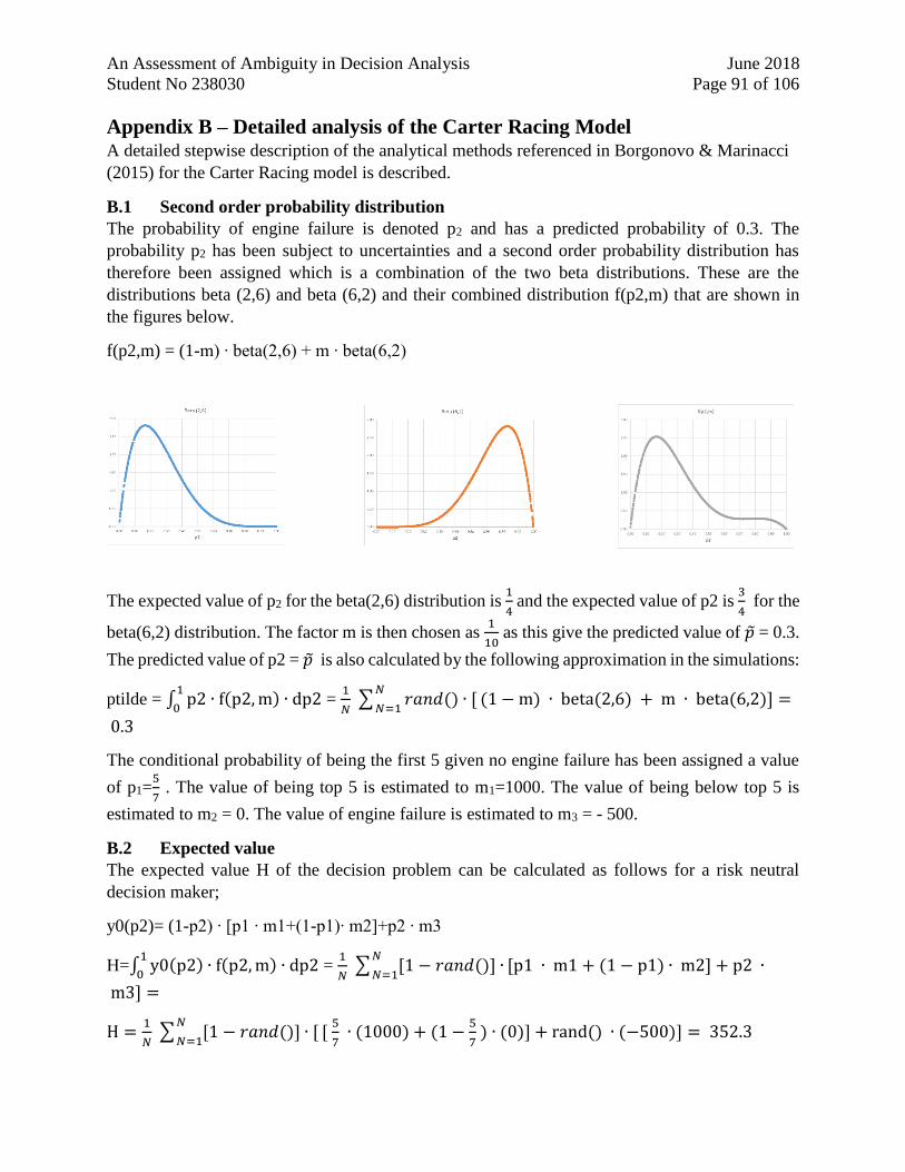
An Assessment of Ambiguity in Decision Analysis June 2018
Student No 238030 Page 91 of 106
Appendix B – Detailed analysis of the Carter Racing Model A detailed stepwise description of the analytical methods referenced in Borgonovo & Marinacci
(2015) for the Carter Racing model is described.
B.1 Second order probability distribution
The probability of engine failure is denoted p2 and has a predicted probability of 0.3. The
probability p2 has been subject to uncertainties and a second order probability distribution has
therefore been assigned which is a combination of the two beta distributions. These are the
distributions beta (2,6) and beta (6,2) and their combined distribution f(p2,m) that are shown in
the figures below.
f(p2,m) = (1-m) ∙ beta(2,6) + m ∙ beta(6,2)
The expected value of p2 for the beta(2,6) distribution is 1
4 and the expected value of p2 is
3
4 for the
beta(6,2) distribution. The factor m is then chosen as 1
10 as this give the predicted value of 𝑝 = 0.3.
The predicted value of p2 = 𝑝 is also calculated by the following approximation in the simulations:
ptilde = ∫ p2 ∙ f(p2, m) ∙ dp2 1
0=
1
𝑁 ∑ 𝑟𝑎𝑛𝑑() ∙ [
𝑁
𝑁=1(1 − m) ∙ beta(2,6) + m ∙ beta(6,2)] =
0.3
The conditional probability of being the first 5 given no engine failure has been assigned a value
of p1=5
7 . The value of being top 5 is estimated to m1=1000. The value of being below top 5 is
estimated to m2 = 0. The value of engine failure is estimated to m3 = - 500.
B.2 Expected value
The expected value H of the decision problem can be calculated as follows for a risk neutral
decision maker;
y0(p2)= (1-p2) ∙ [p1 ∙ m1+(1-p1)∙ m2]+p2 ∙ m3
H=∫ y0(p2) ∙ f(p2, m) ∙ dp21
0 =
1
𝑁 ∑ [1 − 𝑟𝑎𝑛𝑑()] ∙
𝑁
𝑁=1[p1 ∙ m1 + (1 − p1) ∙ m2] + p2 ∙
m3] =
H =1
𝑁 ∑ [1 − 𝑟𝑎𝑛𝑑()] ∙ [
𝑁
𝑁=1[
5
7 ∙ (1000) + (1 −
5
7 ) ∙ (0)] + rand() ∙ (−500)] = 352.3
An Assessment of Ambiguity in Decision Analysis June 2018
Student No 238030 Page 92 of 106
B.3 Risk aversion
A risk averse decision maker will give a lower weighting to positive outcomes and a higher
weighting to negative outcomes. This can be introduced by the use of a negative exponential
function and a risk aversion parameter a. A risk aversion parameter of a = 1
1000 have been used in
the analysis. The utility values then becomes:
u(a,m1)= - 𝑒− 𝑎 ∙𝑚1 = - 𝑒− 1
1000 ∙ 1000
= - 𝑒− 1= - 0.37
u(a,m2)= - 𝑒− 𝑎 ∙𝑚2 = - 𝑒− 1
1000 ∙(0)
= - 𝑒0= - 1.00
u(a,m3)= - 𝑒− 𝑎 ∙𝑚3 = - 𝑒− 1
1000 ∙(−500)
= - 𝑒0.5 = −1.65
The expected utility of the decision problem can then be calculated:
u(p2,a)= ya(p2,a)=(1-p2)∙ [p1 ∙ u(a,m1)+(1-p1) ∙ u(a,m2)] + p2 ∙ u(a,m3)
G(a)=∫ 𝑦𝑎(𝑝2, 𝑎) ∙ 𝑓(𝑝2, 𝑚) ∙ 𝑑𝑝2 1
0=
G(a)= 1
𝑁 ∑ [(1 − 𝑟𝑎𝑛𝑑()) ∙
𝑁
𝑁=1(
5
7 ∙ (−0.37) + (1 −
5
7 ) ∙ (−1.00)) + rand( ) ∙
(−1.65)[(1 − m) ∙ beta(2,6) + m ∙ beta(6,2)] = −0.88
B.4 Wald Maximin Functional
The Wald Maximin Functional is representing an extreme ambiguity averse decision maker. The
Wald Maximin Functional is in this decision problem the same as the utility for the negative
outcome m3.
W=u(a,m3)= - 𝑒− 𝑎 ∙𝑚3 = - 𝑒− 1
1000 ∙(−500)
= - 𝑒0.5 = −1.65
The corresponding certainty equivalent for the maxmin decision maker is therefore:
c(p2,a) = uinv(u(a,m3)= −ln(−𝑢(𝑎,𝑚3))
𝑎= -
1
1000 ln(-1.65) = - 500
B.5 Risk and ambiguity aversion expressed by the KMM utility
Risk and ambiguity aversion are introduced by the risk aversion parameter a = 1
1000 for the utility
function u(p2,a) = ya(p2,a) and the ambiguity aversion parameter b = 1
100 for the second order
utility function v(b,uinv(a,u(p2,a))).
An Assessment of Ambiguity in Decision Analysis June 2018
Student No 238030 Page 93 of 106
c(p2,a) = uinv(a, ya(p2,a)) = − ln(−𝑦𝑎(𝑝2,𝑎))
𝑎=
− ln(−[(1−𝑝2)∙ [𝑝1 ∙ 𝑢(𝑎,𝑚1)+(1−𝑝1)∙ 𝑢(𝑎,𝑚2)]+ 𝑝2 ∙ 𝑢(𝑎,𝑚3)])
𝑎=
c(p2,a) = − ln(−[(1−𝑟𝑎𝑛𝑑())∙ [
5
7 (−0.37)+(1−
5
7) ∙ (−1.00)] + 𝑟𝑎𝑛𝑑() ∙ (−1.65)])
𝑎
c2= ∫ 𝑐(𝑝2, 𝑎)1
0 f(p2,m)dp2 =
1
𝑁 ∑
− ln(−𝑦𝑎(𝑝2,𝑎))
𝑎𝑁𝑁=1 ∙ [(1 − m) ∙ beta(2,6) + m ∙ beta(6,2)] =
c2= 1
𝑁 ∑
− ln(−[(1−𝑝2)∙ [𝑝1 ∙ 𝑢(𝑎,𝑚1)+(1−𝑝1) ∙ 𝑢(𝑎,𝑚2)] + 𝑝2 ∙ 𝑢(𝑎,𝑚3)])
𝑎𝑁𝑁=1 ∙ [(1 − m) ∙ beta(2,6) + m ∙
beta(6,2)] =
c2 = 1
𝑁 ∑
− ln(−[(1−𝑟𝑎𝑛𝑑())∙ [ 5
7 (−0.37)+(1−
5
7) ∙ (−1.00)] + 𝑟𝑎𝑛𝑑() ∙ (−1.65)])
𝑎𝑁𝑁=1 ∙ [(1 − m) ∙ beta(2,6) +
m ∙ beta(6,2)] =
c2 = 159.68
y2(p2,a,b)=v(b, c(p2,a)) = - 𝑒(−𝑏 ∙ 𝑐(𝑝2,𝑎)) = -
𝑒(−𝑏 ∙ − ln(−[(1−𝑟𝑎𝑛𝑑())∙ [
57
(−0.37)+(1−57
) ∙ (−1.00)] + 𝑟𝑎𝑛𝑑() ∙ (−1.65)])
𝑎)
V(a,b)=∫ 𝑦2(𝑝2, 𝑎, 𝑏) ∙1
0 f(p2,m) ∙ dp2=
V(a,b)= ∫ − 𝑒(−𝑏 ∙ − ln(−[(1−𝑟𝑎𝑛𝑑())∙ [
57
(−0.37)+(1−57
) ∙ (−1.00)] + 𝑟𝑎𝑛𝑑() ∙ (−1.65)])
𝑎) ∙
1
0
[(1 − m)beta(2,6) + m ∙
beta(6,2)]dp2=
V(a,b)=1
𝑁 ∑ − 𝑒
(−𝑏 ∙ − ln(−[(1−𝑟𝑎𝑛𝑑( ))∙ [
57
(−0.37)+(1−57
)∙ (−1.00)]+ 𝑟𝑎𝑛𝑑( )∙ (−1.65)])
𝑎)
[(1 −
𝑁
𝑁=11
10) beta(2,6) + (
1
10) beta(6,2)]dp2 = - 4.19
The above method of calculating the KMM utility is similar to the KMM functional for the
Ellsberg three-color problem. Another method is shown below which gives the same result.
φ(p2,b,a)= -(-ya(p2,a)) 𝑏
𝑎
V2(a,b)=∫ 𝜑(𝑝2, 𝑎, 𝑏)𝑓(𝑝2, 𝑚)𝑑𝑝21
0 = ∫ -(-ya(p2,a))
𝑏
𝑎 ∙ [(1 − m)beta(2,6) + m ∙1
0
beta(6,2)]𝑑𝑝2=
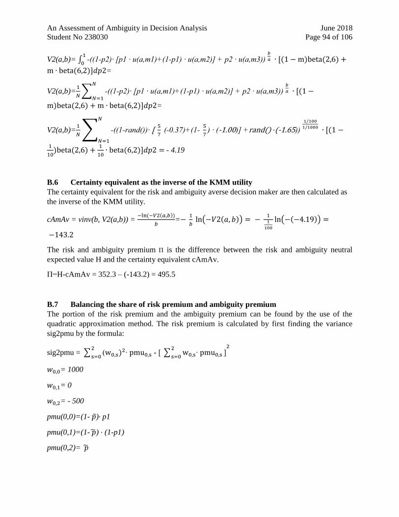
An Assessment of Ambiguity in Decision Analysis June 2018
Student No 238030 Page 94 of 106
V2(a,b)= ∫ -((1-p2)∙ [p1 ∙ u(a,m1)+(1-p1) ∙ u(a,m2)] + p2 ∙ u(a,m3)) 𝑏
𝑎 ∙ [(1 − m)beta(2,6) +1
0
m ∙ beta(6,2)]𝑑𝑝2=
V2(a,b)=1
𝑁∑ -((1-p2)∙ [p1 ∙ u(a,m1)+(1-p1) ∙ u(a,m2)] + p2 ∙ u(a,m3))
𝑏
𝑎 ∙ [(1 −𝑁
𝑁=1
m)beta(2,6) + m ∙ beta(6,2)]𝑑𝑝2=
V2(a,b)=1
𝑁∑ -((1-rand())∙ [
5
7 (-0.37)+(1-
5
7) ∙ (-1.00)] +rand() ∙(-1.65))
1/100
1/1000 ∙ [(1 −
𝑁
𝑁=11
10)beta(2,6) +
1
10∙ beta(6,2)]𝑑𝑝2 = - 4.19
B.6 Certainty equivalent as the inverse of the KMM utility
The certainty equivalent for the risk and ambiguity averse decision maker are then calculated as
the inverse of the KMM utility.
cAmAv = vinv(b, V2(a,b)) = −ln(−𝑉2(𝑎,𝑏))
𝑏=−
1
𝑏 ln(−𝑉2(𝑎, 𝑏)) = −
11
100
ln(−(−4.19)) =
−143.2
The risk and ambiguity premium П is the difference between the risk and ambiguity neutral
expected value H and the certainty equivalent cAmAv.
П=H-cAmAv = 352.3 – (-143.2) = 495.5
B.7 Balancing the share of risk premium and ambiguity premium
The portion of the risk premium and the ambiguity premium can be found by the use of the
quadratic approximation method. The risk premium is calculated by first finding the variance
sig2pmu by the formula:
sig2pmu = ∑ (w0,s)2∙ pmu0,s 2
s=0- [ ∑ w0,s∙ pmu0,s
2
s=0]
2
𝑤0,0= 1000
𝑤0,1= 0
𝑤0,2= - 500
pmu(0,0)=(1- 𝑝)∙ p1
pmu(0,1)=(1- �̃�) ∙ (1-p1)
pmu(0,2)= �̃�
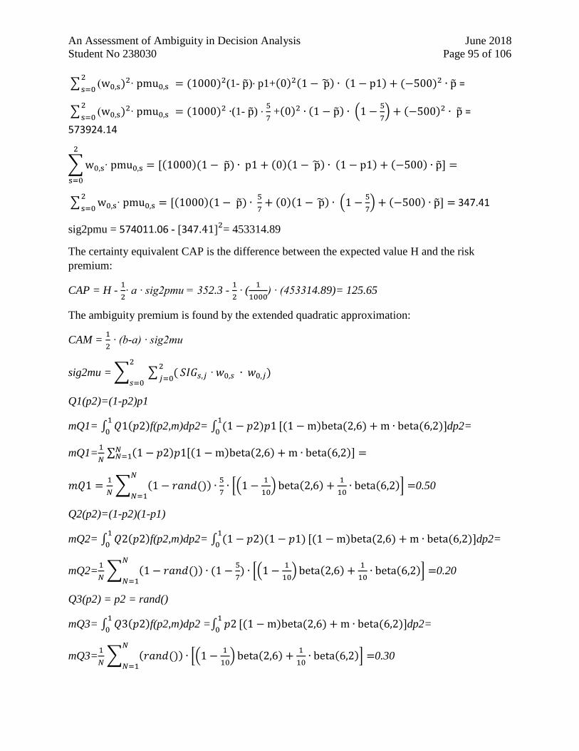
An Assessment of Ambiguity in Decision Analysis June 2018
Student No 238030 Page 95 of 106
∑ (w0,s)2∙ pmu0,s 2
s=0= (1000)2(1- p̃)∙ p1+(0)2(1 − p̃) ∙ (1 − p1) + (−500)2 ∙ p̃ =
∑ (w0,s)2∙ pmu0,s 2
s=0= (1000)2 ∙(1- p̃) ∙
5
7 +(0)2 ∙ (1 − p̃) ∙ (1 −
5
7) + (−500)2 ∙ p̃ =
573924.14
∑ w0,s∙ pmu0,s
2
s=0
= [(1000)(1 − p̃) ∙ p1 + (0)(1 − p̃) ∙ (1 − p1) + (−500) ∙ p̃] =
∑ w0,s∙ pmu0,s2
s=0= [(1000)(1 − p̃) ∙
5
7+ (0)(1 − p̃) ∙ (1 −
5
7) + (−500) ∙ p̃] = 347.41
sig2pmu = 574011.06 - [347.41]2= 453314.89
The certainty equivalent CAP is the difference between the expected value H and the risk
premium:
CAP = H - 1
2∙ a ∙ sig2pmu = 352.3 -
1
2 ∙ (
1
1000) ∙ (453314.89)= 125.65
The ambiguity premium is found by the extended quadratic approximation:
CAM = 1
2 ∙ (b-a) ∙ sig2mu
sig2mu = ∑ ∑ (2
𝑗=0
2
𝑠=0𝑆𝐼𝐺𝑠,𝑗 ∙ 𝑤0,𝑠 ∙ 𝑤0,𝑗)
Q1(p2)=(1-p2)p1
mQ1= ∫ 𝑄1(𝑝2)1
0f(p2,m)dp2= ∫ (1 − 𝑝2)𝑝1
1
0[(1 − m)beta(2,6) + m ∙ beta(6,2)]dp2=
mQ1=1
𝑁 ∑ (1 − 𝑝2)𝑝1[(1 − m)beta(2,6) + m ∙ beta(6,2)] =𝑁
𝑁=1
𝑚𝑄1 =1
𝑁 ∑ (1 − 𝑟𝑎𝑛𝑑()) ∙
5
7∙ [(1 −
1
10) beta(2,6) +
1
10∙ beta(6,2)] =
𝑁
𝑁=10.50
Q2(p2)=(1-p2)(1-p1)
mQ2= ∫ 𝑄2(𝑝2)1
0f(p2,m)dp2= ∫ (1 − 𝑝2)(1 − 𝑝1)
1
0[(1 − m)beta(2,6) + m ∙ beta(6,2)]dp2=
mQ2=1
𝑁 ∑ (1 − 𝑟𝑎𝑛𝑑()) ∙ (1 −
5
7) ∙ [(1 −
1
10) beta(2,6) +
1
10∙ beta(6,2)] =
𝑁
𝑁=10.20
Q3(p2) = p2 = rand()
mQ3= ∫ 𝑄3(𝑝2)1
0f(p2,m)dp2 =∫ 𝑝2
1
0[(1 − m)beta(2,6) + m ∙ beta(6,2)]dp2=
mQ3=1
𝑁 ∑ (𝑟𝑎𝑛𝑑()) ∙ [(1 −
1
10) beta(2,6) +
1
10∙ beta(6,2)] =
𝑁
𝑁=10.30
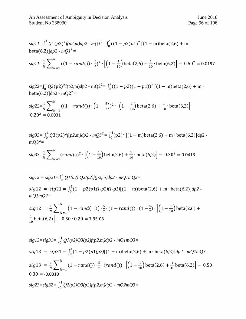
An Assessment of Ambiguity in Decision Analysis June 2018
Student No 238030 Page 96 of 106
sig11=∫ 𝑄1(𝑝2)21
0f(p2,m)dp2 - mQ1
2=∫ ((1 − 𝑝2)𝑝1)21
0[(1 − m)beta(2,6) + m ∙
beta(6,2)]dp2 - mQ12=
sig11=1
𝑁 ∑ ((1 − 𝑟𝑎𝑛𝑑()) ∙
5
7)2 ∙ [(1 −
1
10) beta(2,6) +
1
10∙ beta(6,2)] − 0.502 =
𝑁
𝑁=1 0.0197
sig22=∫ Q2(p2)21
0f(p2,m)dp2 - mQ2
2= ∫ ((1 − 𝑝2)(1 − 𝑝1))21
0[(1 − m)beta(2,6) + m ∙
beta(6,2)]dp2 - mQ22=
sig22=1
𝑁 ∑ ((1 − 𝑟𝑎𝑛𝑑()) ∙ (1 −
5
7))2 ∙ [(1 −
1
10) beta(2,6) +
1
10∙ beta(6,2)] −
𝑁
𝑁=1
0.202 = 0.0031
sig33= ∫ 𝑄3(𝑝2)21
0f(p2,m)dp2 - mQ3
2= ∫ (p2)21
0[(1 − m)beta(2,6) + m ∙ beta(6,2)]dp2 -
mQ32=
sig33=1
𝑁 ∑ (𝑟𝑎𝑛𝑑())2 ∙ [(1 −
1
10) beta(2,6) +
1
10∙ beta(6,2)] − 0.302 =
𝑁
𝑁=1 0.0413
sig12 = sig21=∫ Q1(p2) 1
0Q2(p2)f(p2,m)dp2 - mQ1mQ2=
𝑠𝑖𝑔12 = 𝑠𝑖𝑔21 = ∫ (1 − 𝑝2)𝑝11
0(1-p2)(1-p1)[(1 − m)beta(2,6) + m ∙ beta(6,2)]dp2 -
mQ1mQ2=
𝑠𝑖𝑔12 = 1
𝑁 ∑ (1 − 𝑟𝑎𝑛𝑑( )) ∙
5
7∙ (1 − 𝑟𝑎𝑛𝑑()) ∙ (1 −
5
7) ∙ [(1 −
1
10) beta(2,6) +
𝑁
𝑁=11
10beta(6,2)] − 0.50 ∙ 0.20 = 7.9E-03
sig13=sig31= ∫ Q1(p2)1
0Q3(p2)f(p2,m)dp2 - mQ1mQ3=
𝑠𝑖𝑔13 = 𝑠𝑖𝑔31 = ∫ (1 − 𝑝2)𝑝11
0(p2)[(1 − m)beta(2,6) + m ∙ beta(6,2)]dp2 - mQ1mQ3=
𝑠𝑖𝑔13 = 1
𝑁 ∑ (1 − 𝑟𝑎𝑛𝑑()) ∙
5
7∙ (𝑟𝑎𝑛𝑑()) ∙ [(1 −
1
10) beta(2,6) +
1
10beta(6,2)] − 0.50 ∙
𝑁
𝑁=1
0.30 = -0.0310
sig23=sig32= ∫ Q2(p2)1
0Q3(p2)f(p2,m)dp2 - mQ2mQ3=
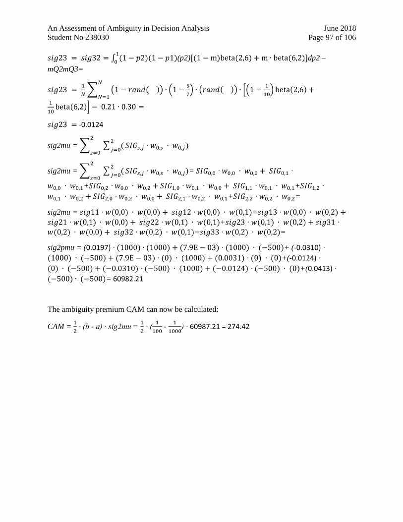
An Assessment of Ambiguity in Decision Analysis June 2018
Student No 238030 Page 97 of 106
𝑠𝑖𝑔23 = 𝑠𝑖𝑔32 = ∫ (1 − 𝑝2)(1 − 𝑝1)1
0(p2)[(1 − m)beta(2,6) + m ∙ beta(6,2)]dp2 –
mQ2mQ3=
𝑠𝑖𝑔23 = 1
𝑁 ∑ (1 − 𝑟𝑎𝑛𝑑( )) ∙ (1 −
5
7) ∙ (𝑟𝑎𝑛𝑑( )) ∙ [(1 −
1
10) beta(2,6) +
𝑁
𝑁=11
10beta(6,2)] − 0.21 ∙ 0.30 =
𝑠𝑖𝑔23 = -0.0124
sig2mu = ∑ ∑ (2
𝑗=0
2
𝑠=0𝑆𝐼𝐺𝑠,𝑗 ∙ 𝑤0,𝑠 ∙ 𝑤0,𝑗)
sig2mu = ∑ ∑ (2
𝑗=0
2
𝑠=0𝑆𝐼𝐺𝑠,𝑗 ∙ 𝑤0,𝑠 ∙ 𝑤0,𝑗)= 𝑆𝐼𝐺0,0 ∙ 𝑤0,0 ∙ 𝑤0,0 + 𝑆𝐼𝐺0,1 ∙
𝑤0,0 ∙ 𝑤0,1+𝑆𝐼𝐺0,2 ∙ 𝑤0,0 ∙ 𝑤0,2 + 𝑆𝐼𝐺1,0 ∙ 𝑤0,1 ∙ 𝑤0,0 + 𝑆𝐼𝐺1,1 ∙ 𝑤0,1 ∙ 𝑤0,1+𝑆𝐼𝐺1,2 ∙
𝑤0,1 ∙ 𝑤0,2 + 𝑆𝐼𝐺2,0 ∙ 𝑤0,2 ∙ 𝑤0,0 + 𝑆𝐼𝐺2,1 ∙ 𝑤0,2 ∙ 𝑤0,1+𝑆𝐼𝐺2,2 ∙ 𝑤0,2 ∙ 𝑤0,2=
sig2mu = 𝑠𝑖𝑔11 ∙ 𝑤(0,0) ∙ 𝑤(0,0) + 𝑠𝑖𝑔12 ∙ 𝑤(0,0) ∙ 𝑤(0,1)+𝑠𝑖𝑔13 ∙ 𝑤(0,0) ∙ 𝑤(0,2) +
𝑠𝑖𝑔21 ∙ 𝑤(0,1) ∙ 𝑤(0,0) + 𝑠𝑖𝑔22 ∙ 𝑤(0,1) ∙ 𝑤(0,1)+𝑠𝑖𝑔23 ∙ 𝑤(0,1) ∙ 𝑤(0,2) + 𝑠𝑖𝑔31 ∙
𝑤(0,2) ∙ 𝑤(0,0) + 𝑠𝑖𝑔32 ∙ 𝑤(0,2) ∙ 𝑤(0,1)+𝑠𝑖𝑔33 ∙ 𝑤(0,2) ∙ 𝑤(0,2)=
sig2pmu = (0.0197) ∙ (1000) ∙ (1000) + (7.9E − 03) ∙ (1000) ∙ (−500)+ (-0.0310) ∙
(1000) ∙ (−500) + (7.9E − 03) ∙ (0) ∙ (1000) + (0.0031) ∙ (0) ∙ (0)+(-0.0124) ∙
(0) ∙ (−500) + (−0.0310) ∙ (−500) ∙ (1000) + (−0.0124) ∙ (−500) ∙ (0)+(0.0413) ∙
(−500) ∙ (−500)= 60982.21
The ambiguity premium CAM can now be calculated:
CAM = 1
2 ∙ (b - a) ∙ sig2mu =
1
2 ∙ (
1
100 -
1
1000) ∙ 60987.21 = 274.42
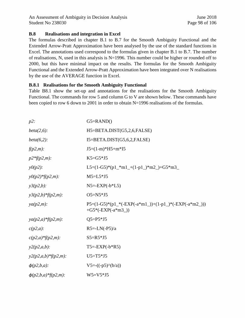
An Assessment of Ambiguity in Decision Analysis June 2018
Student No 238030 Page 98 of 106
B.8 Realisations and integration in Excel
The formulas described in chapter B.1 to B.7 for the Smooth Ambiguity Functional and the
Extended Arrow-Pratt Approximation have been analysed by the use of the standard functions in
Excel. The annotations used correspond to the formulas given in chapter B.1 to B.7. The number
of realisations, N, used in this analysis is N=1996. This number could be higher or rounded off to
2000, but this have minimal impact on the results. The formulas for the Smooth Ambiguity
Functional and the Extended Arrow-Pratt Approximation have been integrated over N realisations
by the use of the AVERAGE function in Excel.
B.8.1 Realisations for the Smooth Ambiguity Functional
Table B8.1 show the set-up and annotations for the realisations for the Smooth Ambiguity
Functional. The commands for row 5 and column G to V are shown below. These commands have
been copied to row 6 down to 2001 in order to obtain N=1996 realisations of the formulas.
p2: G5=RAND()
beta(2,6): H5=BETA.DIST(G5,2,6,FALSE)
beta(6,2): I5=BETA.DIST(G5,6,2,FALSE)
f(p2,m): J5=(1-m)*H5+m*I5
p2*f(p2,m): K5=G5*J5
y0(p2): L5=(1-G5)*(p1_*m1_+(1-p1_)*m2_)+G5*m3_
y0(p2)*f(p2,m): M5=L5*J5
y3(p2,b): N5=-EXP(-b*L5)
y3(p2,b)*f(p2,m): O5=N5*J5
ya(p2,m): P5=(1-G5)*(p1_*(-EXP(-a*m1_))+(1-p1_)*(-EXP(-a*m2_)))
+G5*(-EXP(-a*m3_))
ya(p2,a)*f(p2,m): Q5=P5*J5
c(p2,a): R5=-LN(-P5)/a
c(p2,a)*f(p2,m): S5=R5*J5
y2(p2,a,b): T5=-EXP(-b*R5)
y2(p2,a,b)*f(p2,m): U5=T5*J5
ϕ(p2,b,a): V5=-((-p5)^(b/a))
ϕ(p2,b,a)*f(p2,m): W5=V5*J5
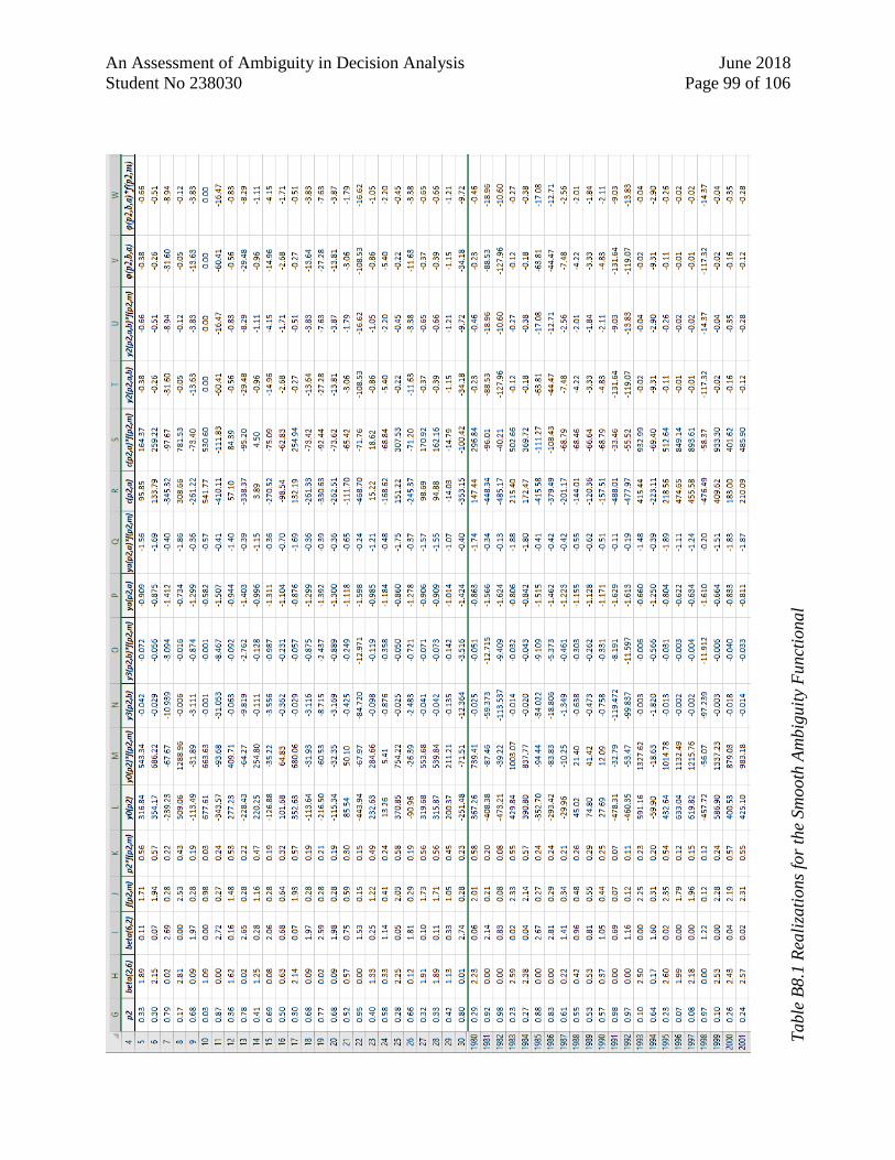
An Assessment of Ambiguity in Decision Analysis June 2018
Student No 238030 Page 99 of 106
Table
B8.1
Rea
liza
tions
for
the
Sm
ooth
Am
big
uit
y F
unct
ional

An Assessment of Ambiguity in Decision Analysis June 2018
Student No 238030 Page 100 of 106
B.8.2 Realisations for the Extended Arrow-Pratt Approximation
The formulas for the Extended Arrow-Pratt Approximation have been analysed by the use of the
standard functions in Excel. Table B8.2 show the set-up and the annotations used where the
commands for row 5 and column X to AI are shown below. These commands have been copied to
row 6 down to row 2001 in order to obtain 1996 realisations of the formulas.
Q1(P2): X5=(1-G5)*p1_
Q1(p2)*f(p2,m): Y5=X5*J5
Q2(p2): Z5=(1-G5)*(1-p1_)
Q2(p2)*f(p2,m): AA5=Z5*J5
Q3(p2): AB5=G5
Q3(p2)*f(p2,m): AC5=AB5*J5
Q1(p2)*Q1(p2)*f(p2,m): AD5=X5*X5*J5
Q2(p2)*Q2(p2)*f(p2,m): AE5=Z5*Z5*J5
Q3(p2)*Q3(p2)*f(p2,m): AF5=AB5*AB5*J5
Q1(p2)*Q2(p2)*f(p2,m): AG5=X5*Z5*J5
Q1(p2)*Q3(p2)*f(p2,.m): AH5=X5*AB5*J5
Q2(p2)*Q3(p2)*f(p2,m): AI5=Z5*AB5*J5
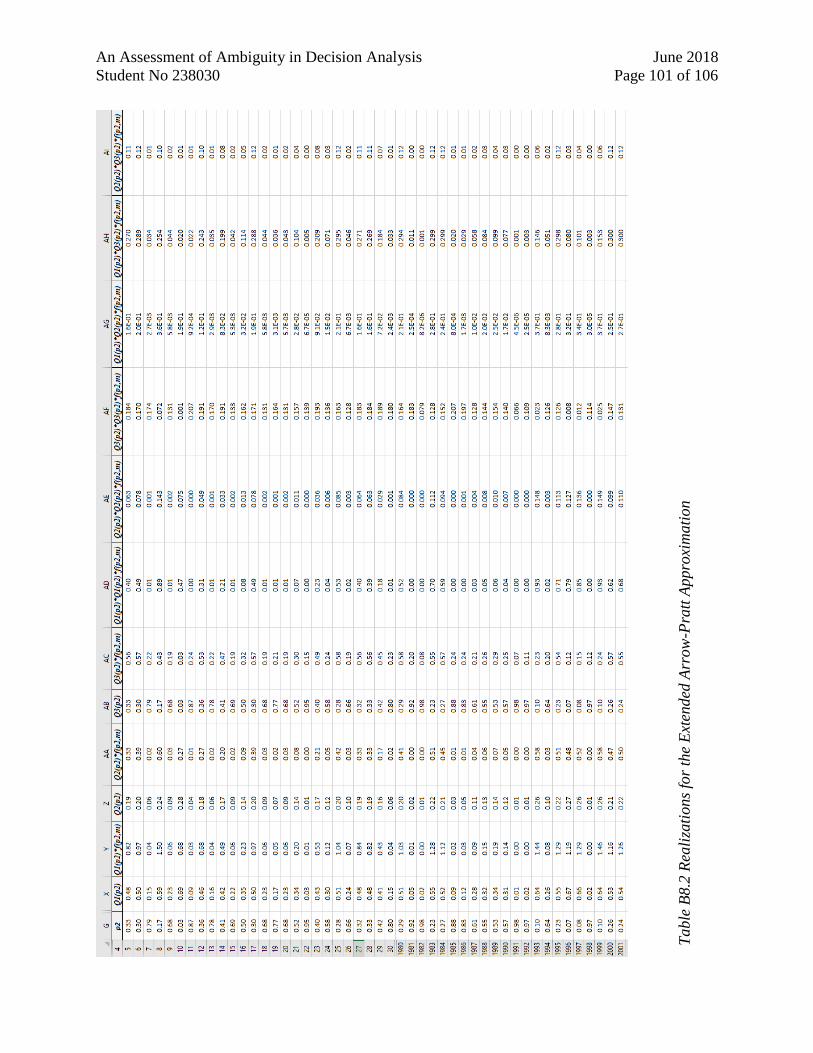
An Assessment of Ambiguity in Decision Analysis June 2018
Student No 238030 Page 101 of 106
Table
B8.2
Rea
liza
tions
for
the
Ext
ended
Arr
ow
-Pra
tt A
ppro
xim
ati
on
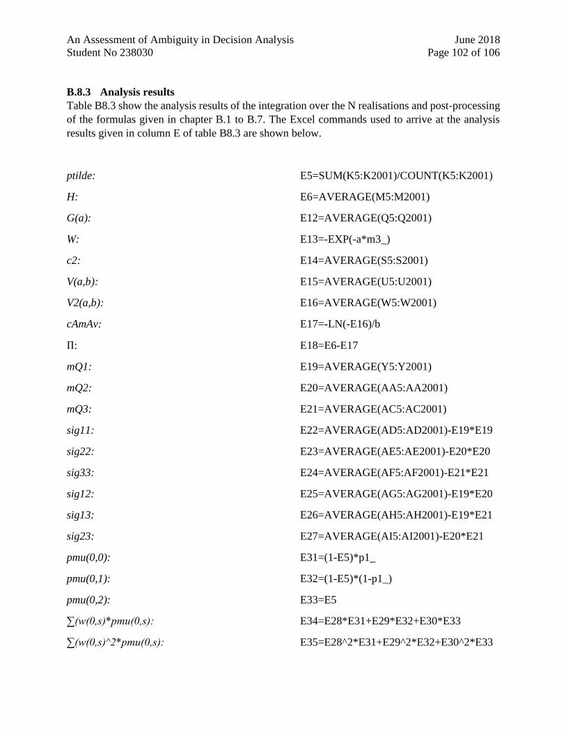
An Assessment of Ambiguity in Decision Analysis June 2018
Student No 238030 Page 102 of 106
B.8.3 Analysis results
Table B8.3 show the analysis results of the integration over the N realisations and post-processing
of the formulas given in chapter B.1 to B.7. The Excel commands used to arrive at the analysis
results given in column E of table B8.3 are shown below.
ptilde: E5=SUM(K5:K2001)/COUNT(K5:K2001)
H: E6=AVERAGE(M5:M2001)
G(a): E12=AVERAGE(Q5:Q2001)
W: E13=-EXP(-a*m3_)
c2: E14=AVERAGE(S5:S2001)
V(a,b): E15=AVERAGE(U5:U2001)
V2(a,b): E16=AVERAGE(W5:W2001)
cAmAv: E17=-LN(-E16)/b
П: E18=E6-E17
mQ1: E19=AVERAGE(Y5:Y2001)
mQ2: E20=AVERAGE(AA5:AA2001)
mQ3: E21=AVERAGE(AC5:AC2001)
sig11: E22=AVERAGE(AD5:AD2001)-E19*E19
sig22: E23=AVERAGE(AE5:AE2001)-E20*E20
sig33: E24=AVERAGE(AF5:AF2001)-E21*E21
sig12: E25=AVERAGE(AG5:AG2001)-E19*E20
sig13: E26=AVERAGE(AH5:AH2001)-E19*E21
sig23: E27=AVERAGE(AI5:AI2001)-E20*E21
pmu(0,0): E31=(1-E5)*p1_
pmu(0,1): E32=(1-E5)*(1-p1_)
pmu(0,2): E33=E5
∑(w(0,s)*pmu(0,s): E34=E28*E31+E29*E32+E30*E33
∑(w(0,s)^2*pmu(0,s): E35=E28^2*E31+E29^2*E32+E30^2*E33
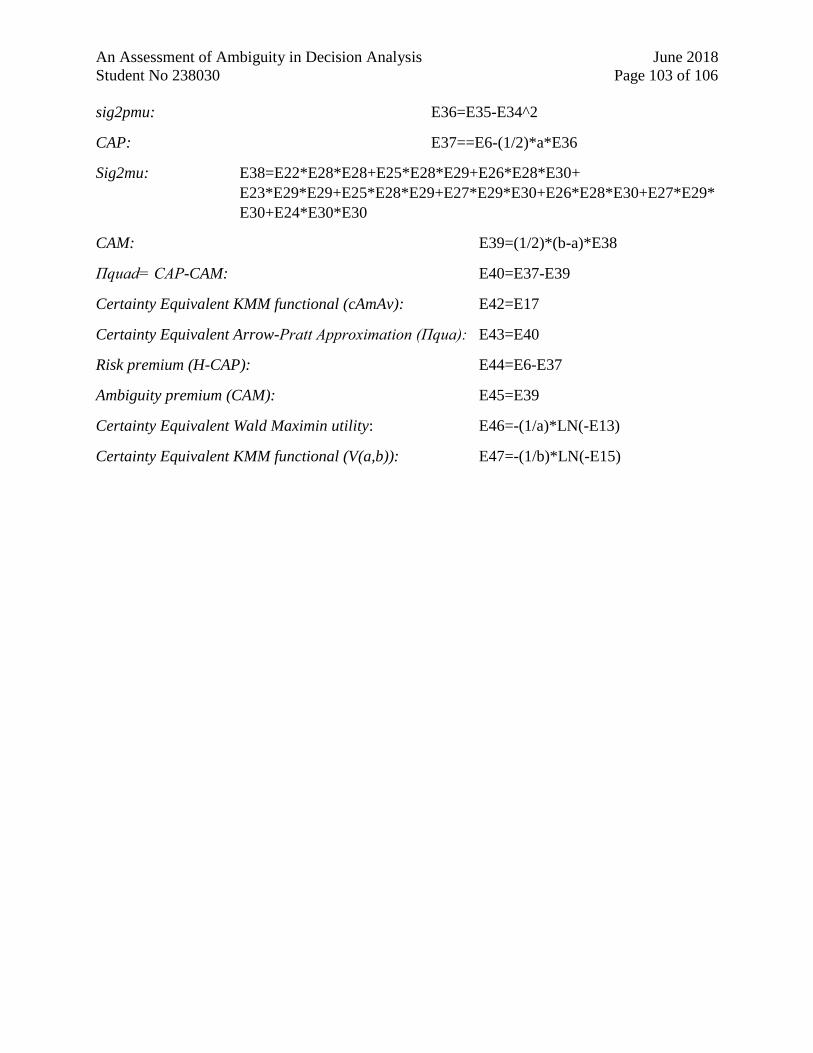
An Assessment of Ambiguity in Decision Analysis June 2018
Student No 238030 Page 103 of 106
sig2pmu: E36=E35-E34^2
CAP: E37==E6-(1/2)*a*E36
Sig2mu: E38=E22*E28*E28+E25*E28*E29+E26*E28*E30+
E23*E29*E29+E25*E28*E29+E27*E29*E30+E26*E28*E30+E27*E29*
E30+E24*E30*E30
CAM: E39=(1/2)*(b-a)*E38
Пquad= CAP-CAM: E40=E37-E39
Certainty Equivalent KMM functional (cAmAv): E42=E17
Certainty Equivalent Arrow-Pratt Approximation (Пqua): E43=E40
Risk premium (H-CAP): E44=E6-E37
Ambiguity premium (CAM): E45=E39
Certainty Equivalent Wald Maximin utility: E46=-(1/a)*LN(-E13)
Certainty Equivalent KMM functional (V(a,b)): E47=-(1/b)*LN(-E15)
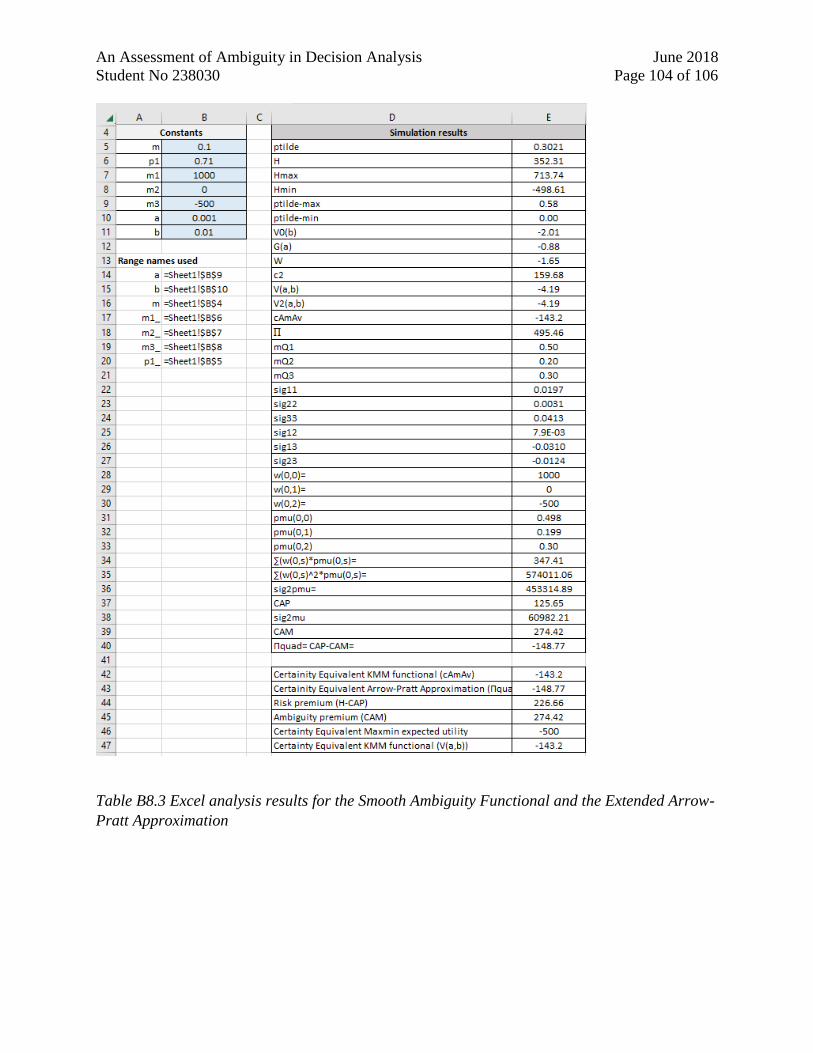
An Assessment of Ambiguity in Decision Analysis June 2018
Student No 238030 Page 104 of 106
Table B8.3 Excel analysis results for the Smooth Ambiguity Functional and the Extended Arrow-
Pratt Approximation
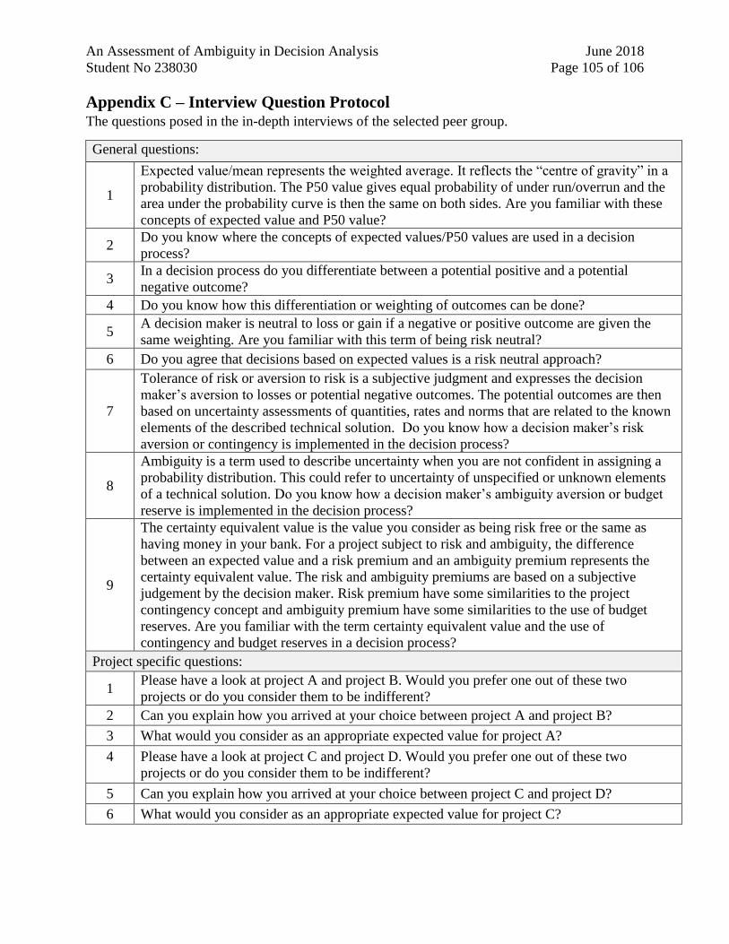
An Assessment of Ambiguity in Decision Analysis June 2018
Student No 238030 Page 105 of 106
Appendix C – Interview Question Protocol The questions posed in the in-depth interviews of the selected peer group.
General questions:
1
Expected value/mean represents the weighted average. It reflects the “centre of gravity” in a
probability distribution. The P50 value gives equal probability of under run/overrun and the
area under the probability curve is then the same on both sides. Are you familiar with these
concepts of expected value and P50 value?
2 Do you know where the concepts of expected values/P50 values are used in a decision
process?
3 In a decision process do you differentiate between a potential positive and a potential
negative outcome?
4 Do you know how this differentiation or weighting of outcomes can be done?
5 A decision maker is neutral to loss or gain if a negative or positive outcome are given the
same weighting. Are you familiar with this term of being risk neutral?
6 Do you agree that decisions based on expected values is a risk neutral approach?
7
Tolerance of risk or aversion to risk is a subjective judgment and expresses the decision
maker’s aversion to losses or potential negative outcomes. The potential outcomes are then
based on uncertainty assessments of quantities, rates and norms that are related to the known
elements of the described technical solution. Do you know how a decision maker’s risk
aversion or contingency is implemented in the decision process?
8
Ambiguity is a term used to describe uncertainty when you are not confident in assigning a
probability distribution. This could refer to uncertainty of unspecified or unknown elements
of a technical solution. Do you know how a decision maker’s ambiguity aversion or budget
reserve is implemented in the decision process?
9
The certainty equivalent value is the value you consider as being risk free or the same as
having money in your bank. For a project subject to risk and ambiguity, the difference
between an expected value and a risk premium and an ambiguity premium represents the
certainty equivalent value. The risk and ambiguity premiums are based on a subjective
judgement by the decision maker. Risk premium have some similarities to the project
contingency concept and ambiguity premium have some similarities to the use of budget
reserves. Are you familiar with the term certainty equivalent value and the use of
contingency and budget reserves in a decision process?
Project specific questions:
1 Please have a look at project A and project B. Would you prefer one out of these two
projects or do you consider them to be indifferent?
2 Can you explain how you arrived at your choice between project A and project B?
3 What would you consider as an appropriate expected value for project A?
4
Please have a look at project C and project D. Would you prefer one out of these two
projects or do you consider them to be indifferent?
5 Can you explain how you arrived at your choice between project C and project D?
6 What would you consider as an appropriate expected value for project C?
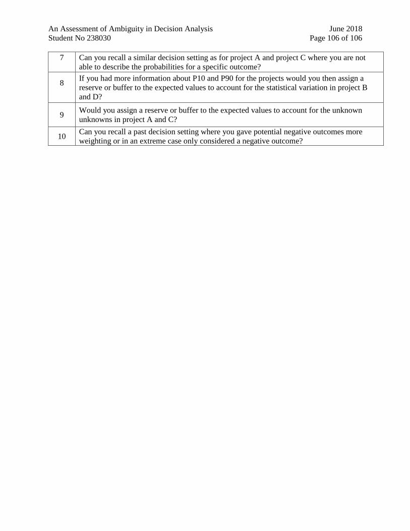
An Assessment of Ambiguity in Decision Analysis June 2018
Student No 238030 Page 106 of 106
7
Can you recall a similar decision setting as for project A and project C where you are not
able to describe the probabilities for a specific outcome?
8
If you had more information about P10 and P90 for the projects would you then assign a
reserve or buffer to the expected values to account for the statistical variation in project B
and D?
9 Would you assign a reserve or buffer to the expected values to account for the unknown
unknowns in project A and C?
10 Can you recall a past decision setting where you gave potential negative outcomes more
weighting or in an extreme case only considered a negative outcome?