Prediction Qualities of the Ifo Indicators on a Temporal Disaggregated German GDP

Christian Seiler

Ifo Working Paper No. 67

February 2009

An electronic version of the paper may be downloaded from the Ifo website www.ifo.de.

Ifo Working Paper No. 67

Prediction Qualities of the Ifo Indicators on a Temporal Disaggregated German GDP

Abstract This paper compares the German Gross Domestic Product between 1991 and 2008 with the Ifo business indicators. Because GDP is published quarterly but the Ifo indicators monthly, the most analyses compare these variables by merging the indicators to quar-terly data. In this paper an alternative way is shown: GDP will be disaggregated with ECOTRIM, a software package from Eurostat, to get monthly data. Furthermore, a spline-based disaggregation approach is discussed. The results of the analyses demon-strate a high connection between the disaggregated GDP and the Ifo indicators. JEL Code: E3. Keywords: Temporal disaggregation, indicators, Gross Domestic Product, splines.

Christian Seiler

Ifo Institute for Economic Research at the University of Munich

Poschingerstr. 5 81679 Munich, Germany

Phone: +49(0)89/9224-1248 seiler@ifo.de

Contents

1 Introduction and motivation 3

2 Disaggregation of GDP 4

2.1 The data set . . . . . . . . . . . . . . . . . . . . . . . . . . . . 4

2.2 Disaggregation methods . . . . . . . . . . . . . . . . . . . . . 4

2.3 Disaggregation with ECOTRIM . . . . . . . . . . . . . . . . . 5

2.4 An approach with spline-based weights . . . . . . . . . . . . . 6

3 Comparison 9

3.1 Comparison with the Ifo Business Climate Index . . . . . . . . 10

3.2 Comparison with the Ifo Business Assessment Index . . . . . . 12

3.3 Comparison with the Ifo Business Expectation Index . . . . . 14

4 Summary and outlook 16

A Correlation tables 18

2

1 Introduction and motivation

A great variety of papers about the qualities of the Ifo indicators and their

connection to the German economic cycle exists in the literature; for re-

cent years see for example Fritsche (1999), Kunkel (2003) and Abberger and

Nierhaus (2007). In these analyses the Ifo indicators, which are published

monthly, will be aggregated to quarterly data to compare them with German

GDP, as it is released quarterly. Other analyses, such as Hott et al. (2004),

use industrial production as a reference series to enable a monthly compari-

son.

To overcome the restriction of creating quarterly indices (and probably losing

information), the comparison will be considered from another perspective. In

this paper GDP will be disaggregated to monthly data. This approach bears

a risk because information is created and not measured. However, even an

aggregation of an indicator leads to distortions. The advantage of disag-

gregation is obvious and simple because more data points can be used for

the analysis, and the statements about the indicators can be created more

specifically.

Section 2 gives a brief overview of the data set and different disaggrega-

tion methods. Also a spline-based approach will be discussed in this section.

In section 3 the three most important Ifo indicators are compared with GDP

3

growth rates. Section 4 summarizes the results of this paper and gives an

outlook.

2 Disaggregation of GDP

2.1 The data set

In this analysis German GDP adjusted for price to the basis year 2000, similar

to Kunkel (2003)1, is used. GDP for reunified Germany is available since the

first quarter of 1991 and is published by the Federal Statistical Office of

Germany. The values before 1991 are excluded from the analysis because

they only exist for West Germany, so they range from 1/1991 to 6/2008.

Since GDP is a cumulative value, the method of disaggregation must fulfill

the condition

GDPi = GDP(i,1) + GDP(i,2) + GDP(i,3) (1)

with GDP(i,1), . . . , GDP(i,3) as the appropriate monthly GDPs of quarter i.

Condition (1) characterizes German GDP as a flow series.

2.2 Disaggregation methods

In the literature many different approaches for temporal disaggregation are

found. According to Di Fonzo (2003) most approaches can be classified into

1Note that Kunkel (2003) uses German GDP adjusted for price to the basis year 1995.

4

methods using related indicators and those not using them. Approaches

without such indicators are purely mathematical methods to create a smooth

path for the unobserved series. First methods based on minimizing squared

first or second differences of the high-frequency series were discussed by Boot

et al. (1967); Lisman and Sandee (1964) proposed a set of weights that could

be used to generate high-freqeuncy data. Recent approaches, as in Wei and

Stram (1990) use an ARIMA-based illustration of the time series. In contrast

to these approaches the literature about methods using related indicators

is much larger. These methods calculate the unobserved series using the

information of a related indicator with target frequency. First approaches

have been formulated by Denton (1971), Ginsburgh (1973) and Chow and

Lin (1971). ARIMA-based approaches with related indicators are discussed

in Guerrero (1990) and Wei and Stram (1990); for example.

2.3 Disaggregation with ECOTRIM

For disaggregation of GDP the software tool ECOTRIM Version 1.012 from

Eurostat is used. ECOTRIM includes unvariate as well as multivariate meth-

ods with optional including of related indicators to disaggregate a time series;

see Barcellan and Buono (2002) for further details. In this paper disag-

gregation approaches without a related indicator, i.e. purely mathematical

2ECOTRIM can be downloaded viahttp://circa.europa.eu/Public/irc/dsis/ecotrim/library

5

methods, are used. The first applied method3 was introduced by Boot et al.

(1967). First of all, the monthly values will be set to 1/3 of the quarterly

value. Then the squared first

n∑i=2

(xi − xi−1)2

or second

n∑i=2

(∆xi − ∆xi−1)2

order differences between two successive months xi and xi−1 with ∆xi =

xi+1 − xi will be minimized. The minimization of the differences causes the

course of the quarterly values to be adjusted. Boot et al. (1967) apply their

approach to annual data, but the methodical transfer from “annual to quar-

terly” to “quarterly to monthly” is trivial and provided by ECOTRIM. Both

techniques fulfill condition (1) analogous for annual data.

2.4 An approach with spline-based weights

As in Lisman and Sandee (1964) a flow series can also be disaggregated by

creating a set of weights, e.g. with 1/3 of the quarterly value for the monthly

3Denton’s (1971) method for flow series without using realted indicators is also providedby ECOTRIM. This approach will not be discussed in this paper, because for h = 1 theresults are the same as FD and similar for bigger values of h.

6

data. As mentioned in Jacobs (1994), this method is a very naive way of

disaggregation. Generally, a continuous density function f(i−1,i](t) on each

intervall (i− 1, i] for distributing the i-th GDP can be defined. With setting

c(i,j) as the lower cutpoint of GDP(i,j) the weights are defined as

w(i,j) =

∫ c(i,j+1)

c(i,j)

f(i−1,i](t).

In this paper the cutpoints are set to i − 1, i − 1 + 13, i − 1 + 2

3and i, so

that the c(i,j) are equidistant. The reason is that the months have nearly the

same length.

To estimate the shape of each density function f(i−1,i](t), the time series will

be interpolated and the form of the appropriate piece s(i−1,i](t), i−1 < t < i,

of the interpolated spline function s(t) is used. For interpolation, cubic

splines as descibed in Forsythe et al. (1977) are used. The cubic splines

have different advantages over other interpolation methods, e.g. polynomial

interpolation. Polynomial splines are highly oscillating when the degree of

the polynom rises. Piecewise linear interpolation is also possible, but the

supposed “smoothed” run of GDP isn’t illustrated very well. For general

information about interpolation methodsl; see Stoer and Bulirsch (2002).

To use the spline pieces for the shape of the density function it must be se-

cured that f(i−1,i](t) is a real density function with∫ i

i−1f(i−1,i](t) = 1. There-

7

fore the spline piece s(i−1,i](t) cannot be used directly and must divided by

its own integral, respectively

f(i−1,i](t) =s(i−1,i](t)∫ i

i−1s(i−1,i](t)

. (2)

The resulting monthly GDPs are displayed in figure 1. As you can see,

the calculated values between FD and SD, do not differentiate very largely,

except on the borders. The spline-based method generates values that differ

more than the other two methods.

1992 1994 1996 1998 2000 2002 2004 2006 2008

2530

3540 FD

SDspline−based weights

Figure 1: disaggregated GDP

8

3 Comparison

The Ifo indicators, especially the Business Climate Index (BCI), are widely

observed in Germany and foreign countries. The Ifo BCI is the indexed

geometric mean of the balances4 of the Business Assessment (BA) and the

balances of the Business Expectations (BE), or to be more precise:

BCI = 100 ·√

(BA + 200) · (BE + 200)

BC2000

with BC2000 as the average balances of the year 2000. The subindicators BAI

and BEI are constructed by adding 200 to the balances and indexing them to

the basis year 2000. The Ifo BAI measures the assessment of the actual busi-

ness situation of the companies whereas the Ifo BEI measures the expected

assessment of the companies for the next six months. Both indicators will

be explained in detail, in section 3.2 and 3.3. The indicators are constructed

to measure the cyclical development of economic performance in Germany.

For this reason the main target of the indicators is to detect the growth rate

of German GDP. The Federal Statistical Office of Germany calculates the

growth rates of GDP based on the quarter of the previous year. Analogous

to this approach the growth rates with a basis in the previous years’ month

are calculated.

To enable a comparison with analyses from a quarterly perspective, the cor-

4The balances are constructed by subtracting the negative reponses from the positive.

9

relations of the indicators with the quarterly growth rates were calculated

and listed in Table 4. The results of Kunkel (2003) cannot be used directly

for the comparison, because, although only drawing a small distinction, he

calculates with balances and not with the indicators and his data range from

1/1991 to 4/2002. The comparison with the quarterly values will be discussed

in the corresponding section.

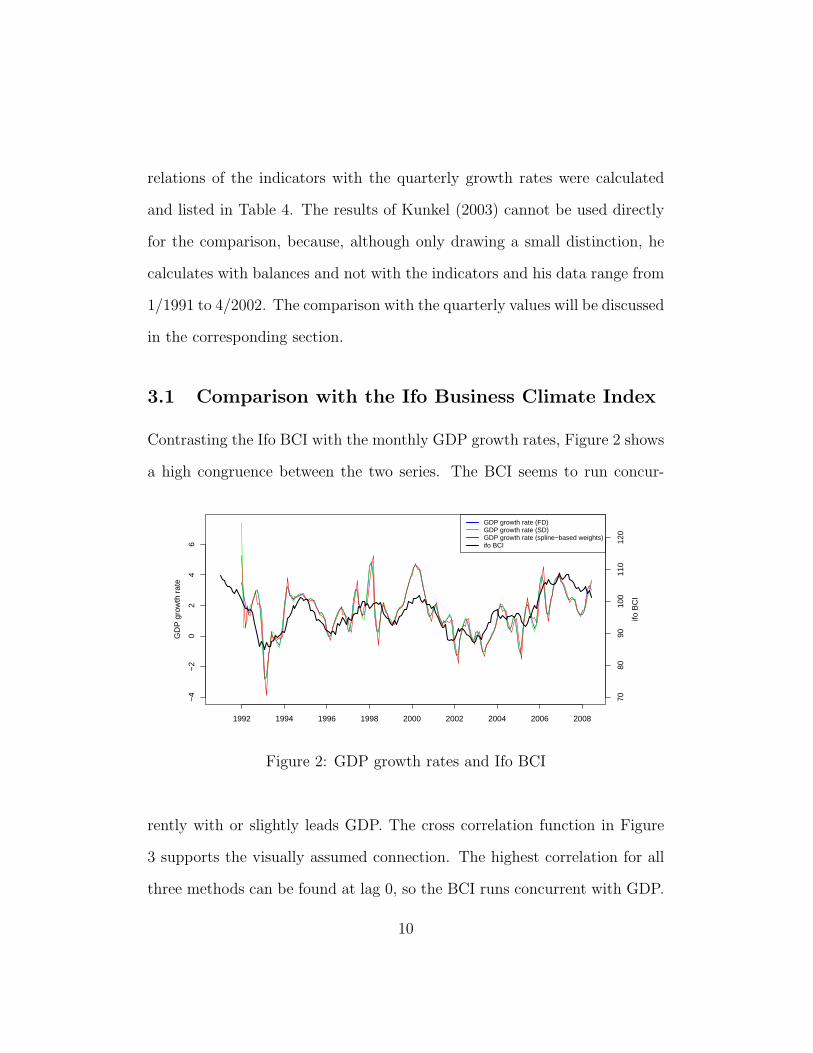
3.1 Comparison with the Ifo Business Climate Index

Contrasting the Ifo BCI with the monthly GDP growth rates, Figure 2 shows

a high congruence between the two series. The BCI seems to run concur-

1992 1994 1996 1998 2000 2002 2004 2006 2008

−4

−2

02

46

GD

P g

row

th r

ate

ifo B

CI

7080

9010

011

012

0

GDP growth rate (FD)GDP growth rate (SD)GDP growth rate (spline−based weights)ifo BCI

Figure 2: GDP growth rates and Ifo BCI

rently with or slightly leads GDP. The cross correlation function in Figure

3 supports the visually assumed connection. The highest correlation for all

three methods can be found at lag 0, so the BCI runs concurrent with GDP.

10

These correlations are also nearly equal for all three methods; see Table

1. It is remarkable that the correlation, for FD as well as for SD and the

spline-based method, until lead 7 is always higher than the correlation to the

corresponding month. The indicator seems to have a closer connection to the

future than to the past. It should be noted that the absolute correlations for

the SD method are almost everywhere lower than those for the FD method.

−18 −12 −6 0 6 12 18

−0.

6−

0.4

−0.

20.

00.

20.

40.

6

FDSDspline−based weights

Figure 3: Cross correlation between GDP growth rates and Ifo BCI

Calculating the quarterly cross correlations, the analysis shows that the high-

est correlation is measured at lag 0, but the correlation is somewhat higher;

see Table 4. So even from this perspective the indicator can be classified as

concurrent. Note that the results of lead 1 to 3, for example, in the monthly

perspective are not exactly like the results of lead 1 in the quarterly perspec-

tive, because the correlation depends on the position of the month in the

11

quarter.

3.2 Comparison with the Ifo Business Assessment In-

dex

For the constructing of the BAI, the companies are asked if their actual busi-

ness situation in this month is good, satisfactory or poor. Interviews and

regression analyses show that the growth of exchange, the number of em-

ployed and/or a combination of these variables affects the business situation;

see Oppenlander and Poser (1989).

1992 1994 1996 1998 2000 2002 2004 2006 2008

−4

−2

02

46

GD

P g

row

th r

ate

ifo B

AI

7080

9010

011

012

0

GDP growth rate (FD)GDP growth rate (SD)GDP growth rate (spline−based weights)ifo BAI

Figure 4: GDP growth rates and Ifo BAI

The BAI is displayed in Figure 4. Visually the indicator seems to run con-

current, especially after 2001. The cross correlation function in Figure 5

12

supports the assumption. The highest correlation is measured at lag 0 for

the spline-based method and at lag 1 for FD and SD; see Table 2. Until 15

months the “lead-correlation” is always higher than the corresponding “lag-

correlation”. This results support the conception that the BAI has a higher

connection to the past than to the future.

−18 −12 −6 0 6 12 18

−0.

6−

0.4

−0.

20.

00.

20.

40.

6

FDSDspline−based weights

Figure 5: Cross correlation between GDP growth rates and Ifo BAI

In the quarterly analyses the BAI has the highest correlation at lag 0 and

would be classified as a concurrent indicator in this perspective. Although

no lag-structure could be measured, the ”lag-correlations” up to 5 quarters

are ever higher; see Table 4.

13

3.3 Comparison with the Ifo Business Expectation In-

dex

The questions for BEI are similarly constructed to those of the BAI. The

companies are asked if their business situation in the next six months will

be good, satisfactory or poor. This question is directed to the future and

marked by high uncertainness.

1992 1994 1996 1998 2000 2002 2004 2006 2008

−4

−2

02

46

GD

P g

row

th r

ate

ifo B

EI

7080

9010

011

012

0

GDP growth rate (FD)GDP growth rate (SD)GDP growth rate (spline−based weights)ifo BEI

Figure 6: GDP growth rates and Ifo BEI

Figure 6 shows the BEI and the monthly GDP growth rates. A clear fore-

running of the indicator can be detected, especially in the periods of 1992 to

1994 and 2002 to 2004. The cross correlation function displayed in Figure

7 supports this visually assumed connection. The highest correlation for all

three methods is measured at lead 3. This can be interpreted such, that the

14

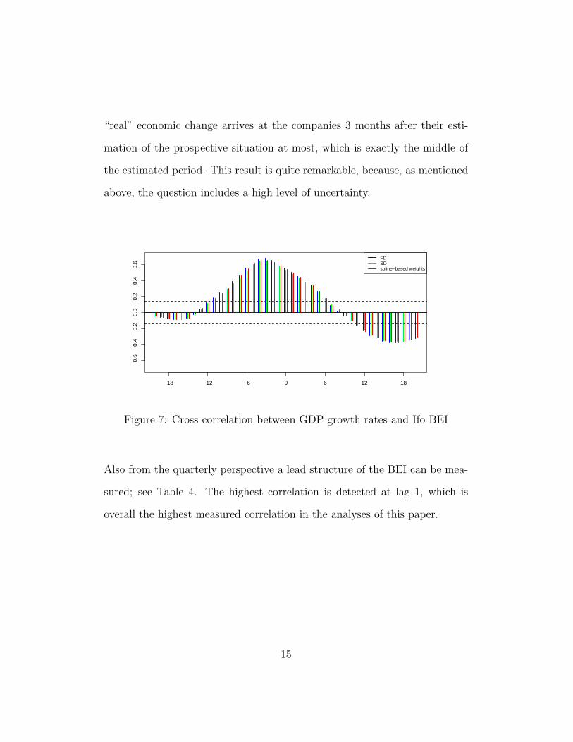
“real” economic change arrives at the companies 3 months after their esti-

mation of the prospective situation at most, which is exactly the middle of

the estimated period. This result is quite remarkable, because, as mentioned

above, the question includes a high level of uncertainty.

−18 −12 −6 0 6 12 18

−0.

6−

0.4

−0.

20.

00.

20.

40.

6

FDSDspline−based weights

Figure 7: Cross correlation between GDP growth rates and Ifo BEI

Also from the quarterly perspective a lead structure of the BEI can be mea-

sured; see Table 4. The highest correlation is detected at lag 1, which is

overall the highest measured correlation in the analyses of this paper.

15

4 Summary and outlook

The analysis in this paper show that there is a close connection between the

Ifo indicators and disaggregated German GDP. The highest correlation of all

three indicators is around 0.65, which is a high value for a latent variable like

the economic performance. The BCI as well as its components, the BAI and

the BEI, have a high correlation with the monthly GDP growth rate and con-

firm the results of several analyses from a quarterly perspective. Especially

the results for the BEI show that the construction of the question about the

prospective business assessment measures is correct. Also the BAI, which

has a closer connection to past than to the future, confirms the idea that the

companies react to the economic situation directly or with a slight delay.

Additionally, the analysis shows that the results depend only marginally on

the chosen method of disaggregation, and, that the correlations with SD are

lower than those with FD. It should be noted that analyses that exclude the

values of 1992 lead to higher correlations. The values before 1992 are some

what critical because on the one hand the disaggregation methods produce

very different values at the beginning of the time series and on the other

hand the values of the indicators shortly after reunification are afflicted with

a slightly higher degree of uncertainty.

The analyses also show that the disaggregation method with spline-based

16

weights presented here leads to reasonable and similar results as with the FD

and the SD method. In a next step the influence of the diverse interpolation

methods should be analysed, embedding them into a mathematical theory.

Moreover, for example by using simluation studies, it should be investigated

whether this method may yield better results than the other methods.

17

A Correlation tables

FD SD splinelead lag lead lag lead lag

0 0.674 0.674 0.644 0.644 0.662 0.6621 0.672 0.659 0.628 0.627 0.651 0.6462 0.663 0.636 0.625 0.605 0.635 0.6193 0.648 0.606 0.615 0.578 0.626 0.5914 0.613 0.566 0.584 0.540 0.596 0.5535 0.561 0.518 0.534 0.497 0.549 0.5086 0.494 0.461 0.468 0.446 0.486 0.4527 0.420 0.402 0.397 0.388 0.412 0.3948 0.346 0.350 0.326 0.341 0.338 0.3529 0.277 0.297 0.260 0.288 0.269 0.29410 0.211 0.238 0.199 0.222 0.207 0.22911 0.149 0.170 0.140 0.165 0.146 0.15912 0.091 0.093 0.086 0.089 0.090 0.08213 0.043 0.021 0.041 0.015 0.044 0.01714 0.008 -0.038 0.006 -0.036 0.007 -0.03315 -0.012 -0.091 -0.013 -0.090 -0.012 -0.09116 -0.017 -0.136 -0.018 -0.134 -0.024 -0.13717 -0.014 -0.173 -0.013 -0.166 -0.019 -0.17318 -0.009 -0.204 -0.007 -0.196 -0.012 -0.19919 -0.006 -0.226 -0.004 -0.214 -0.006 -0.22120 0.000 -0.243 0.000 -0.234 0.002 -0.238

Table 1: Correlations between GDP growth rates and the BCI

18

FD SD splinelead lag lead lag lead lag

0 0.639 0.639 0.611 0.611 0.630 0.6301 0.604 0.646 0.560 0.613 0.586 0.6282 0.568 0.639 0.532 0.607 0.544 0.6203 0.531 0.623 0.503 0.597 0.514 0.6074 0.487 0.601 0.463 0.573 0.474 0.5885 0.437 0.577 0.415 0.551 0.427 0.5676 0.383 0.548 0.363 0.525 0.375 0.5367 0.327 0.515 0.311 0.492 0.317 0.5068 0.271 0.483 0.256 0.465 0.262 0.4799 0.215 0.443 0.202 0.427 0.209 0.43510 0.156 0.392 0.148 0.373 0.158 0.38111 0.102 0.332 0.095 0.322 0.104 0.32112 0.058 0.261 0.055 0.250 0.057 0.24913 0.034 0.193 0.031 0.180 0.030 0.18614 0.023 0.134 0.020 0.129 0.017 0.13415 0.021 0.077 0.019 0.073 0.021 0.07616 0.023 0.023 0.022 0.019 0.017 0.02017 0.027 -0.027 0.027 -0.025 0.022 -0.02918 0.029 -0.075 0.028 -0.072 0.026 -0.07419 0.026 -0.118 0.025 -0.111 0.028 -0.11620 0.025 -0.158 0.023 -0.152 0.028 -0.158

Table 2: Correlations between GDP growth rates and the BAI

19

FD SD splinelead lag lead lag lead lag

0 0.556 0.556 0.531 0.531 0.541 0.5411 0.613 0.505 0.582 0.481 0.594 0.5012 0.657 0.456 0.624 0.436 0.629 0.4473 0.683 0.406 0.650 0.385 0.658 0.3984 0.674 0.344 0.643 0.328 0.653 0.3365 0.631 0.268 0.602 0.260 0.620 0.2636 0.559 0.178 0.530 0.181 0.554 0.1767 0.472 0.090 0.446 0.095 0.472 0.0898 0.387 0.019 0.363 0.029 0.384 0.0339 0.313 -0.043 0.294 -0.036 0.304 -0.03410 0.251 -0.101 0.237 -0.105 0.237 -0.10411 0.191 -0.164 0.180 -0.160 0.179 -0.17412 0.121 -0.230 0.115 -0.220 0.121 -0.23713 0.045 -0.290 0.043 -0.281 0.055 -0.28714 -0.025 -0.331 -0.024 -0.316 -0.016 -0.31915 -0.070 -0.362 -0.069 -0.353 -0.070 -0.35916 -0.087 -0.378 -0.086 -0.368 -0.092 -0.37517 -0.085 -0.383 -0.082 -0.367 -0.087 -0.37818 -0.076 -0.374 -0.070 -0.360 -0.077 -0.36319 -0.064 -0.354 -0.057 -0.337 -0.066 -0.34520 -0.046 -0.325 -0.044 -0.315 -0.048 -0.314

Table 3: Correlations between GDP growth rates and the BEI

BCI BAI BEIlead lag lead lag lead lag

0 0.696 0.696 0.658 0.658 0.582 0.5821 0.666 0.624 0.548 0.639 0.703 0.4272 0.509 0.478 0.396 0.566 0.579 0.1893 0.292 0.305 0.227 0.454 0.332 -0.0444 0.101 0.098 0.067 0.270 0.135 -0.2415 0.001 -0.086 0.032 0.085 -0.059 -0.3696 0.000 -0.205 0.038 -0.073 -0.072 -0.3847 0.012 -0.250 0.033 -0.189 -0.033 -0.2938 0.063 -0.199 0.079 -0.220 0.013 -0.102

Table 4: Correlations between quarterly GDP growth rates and the Ifo indi-cators

20

References

K. Abberger and W. Nierhaus. Das ifo Geschaftsklima und Wendepunkte

der deutschen Konjunktur. ifo Schnelldienst, 60(3), 2007.

R. Barcellan and D. Buono. ECOTRIM Interface. Eurostat, 2002.

J.C.G. Boot, W. Feibes, and J.H.C. Lisman. Further Methods of Derivation

of Quarterly Figures from Annual Data. Applied Statistics, 16(1):65–75,

1967.

G. Chow and A.L. Lin. Best linear unbiased interpolation, distribution and

extrapolation of time series by related series. The Review of Economics

and Statistics, 53:372–375, 1971.

F.T. Denton. Adjustment of monthly or quarterly series to annual Totals:

An Approach based on quadratic Minimization. Journal of the American

Statistical Association, 66, 1971.

T. Di Fonzo. Temporal disaggregation of economic time series: towards a

dynamic extension. Technical report, Dipartimento di Scienze Statistiche,

Universita di Padova, 2003.

G.E. Forsythe, M.A. Malcolm, and C.B. Moler. Computer Methods for Math-

ematical Computations. Prentice Hall, Englewoods Cliffs, 1977.

U. Fritsche. Vorlaufeigenschaften von ifo-Indikatoren fur Westdeutschland.

DIW discussion papers, 179, 1999.

21

V.A. Ginsburgh. A further note on the derivation of quarterly figures con-

sistent with annual data. Applied Statistics, 22:368–374, 1973.

V. Guerrero. Temporal Disaggregation of time Series: An ARIMA-based

Approach. International Statistical Review, 58:29––46, 1990.

C. Hott, A. Kunkel, and G. Nerb. Die Eignung des ifo Geschaftsklimas zur

Prognose von konjunkturellen Wendepunkten, pages 334–358. 2004.

J. Jacobs. ‘Dividing by 4’: a feasible quarterly forecasting method? Technical

report, Department of Economics, University of Groningen, 1994.

A. Kunkel. Zur Prognosefahigkeit des ifo Geschaftsklimas und seiner Kompo-

nenten sowie die Uberprufung der ’Dreimal-Regel’. ifo discussion papers,

80, 2003.

J. Lisman and J. Sandee. Derivation of Quarterly Figures from Annual Data.

Journal of the Royal Statistical Society - Series C, 13:87–90, 1964.

K.H. Oppenlander and G. Poser. Handbuch der ifo Umfragen. Duncker und

Humblot, 1989.

J. Stoer and R. Bulirsch. Introduction to Numerical Analysis. Springer-

Verlag, 2002.

W.W.S. Wei and D.O. Stram. Disaggregation of time series models. Journal

of the Royal Statistical Society - Series B, 52:453–467, 1990.

22

Ifo Working Papers No. 66 Buettner, T. and A. Ebertz, Spatial Implications of Minimum Wages, February 2009. No. 65 Henzel, S. and J. Mayr, The Virtues of VAR Forecast Pooling – A DSGE Model Based

Monte Carlo Study, January 2009. No. 64 Czernich, N., Downstream Market structure and the Incentive for Innovation in Telecom-

munication Infrastructure, December 2008. No. 63 Ebertz, A., The Capitalization of Public Services and Amenities into Land Prices –

Empirical Evidence from German Communities, December 2008. No. 62 Wamser, G., The Impact of Thin-Capitalization Rules on External Debt Usage – A Pro-

pensity Score Matching Approach, October 2008. No. 61 Carstensen, K., J. Hagen, O. Hossfeld and A.S. Neaves, Money Demand Stability and

Inflation Prediction in the Four Largest EMU Countries, August 2008. No. 60 Lahiri, K. and X. Sheng, Measuring Forecast Uncertainty by Disagreement: The Missing

Link, August 2008. No. 59 Overesch, M. and G. Wamser, Who Cares about Corporate Taxation? Asymmetric Tax

Effects on Outbound FDI, April 2008. No. 58 Eicher, T.S: and T. Strobel, Germany’s Continued Productivity Slump: An Industry

Analysis, March 2008. No. 57 Robinzonov, N. and K. Wohlrabe, Freedom of Choice in Macroeconomic Forecasting:

An Illustration with German Industrial Production and Linear Models, March 2008. No. 56 Grundig, B., Why is the share of women willing to work in East Germany larger than in

West Germany? A logit model of extensive labour supply decision, February 2008. No. 55 Henzel, S., Learning Trend Inflation – Can Signal Extraction Explain Survey Forecasts?,

February 2008.

No. 54 Sinn, H.-W., Das grüne Paradoxon: Warum man das Angebot bei der Klimapolitik nicht vergessen darf, Januar 2008.

No. 53 Schwerdt, G. and J. Turunen, Changes in Human Capital: Implications for Productivity

Growth in the Euro Area, December 2007. No. 52 Berlemann, M. und G. Vogt, Kurzfristige Wachstumseffekte von Naturkatastrophen – Eine

empirische Analyse der Flutkatastrophe vom August 2002 in Sachsen, November 2007. No. 51 Huck, S. and G.K. Lünser, Group Reputations – An Experimental Foray, November 2007. No. 50 Meier, V. and G. Schütz, The Economics of Tracking and Non-Tracking, October 2007. No. 49 Buettner, T. and A. Ebertz, Quality of Life in the Regions – Results for German Counties,

September 2007. No. 48 Mayr, J. and D. Ulbricht, VAR Model Averaging for Multi-Step Forecasting, August 2007. No. 47 Becker, S.O. and K. Wohlrabe, Micro Data at the Ifo Institute for Economic Research –

The “Ifo Business Survey”, Usage and Access, August 2007. No. 46 Hülsewig, O., J. Mayr and S. Sorbe, Assessing the Forecast Properties of the CESifo World

Economic Climate Indicator: Evidence for the Euro Area, May 2007. No. 45 Buettner, T., Reform der Gemeindefinanzen, April 2007. No. 44 Abberger, K., S.O. Becker, B. Hofmann und K. Wohlrabe, Mikrodaten im ifo Institut – Be-

stand, Verwendung und Zugang, März 2007. No. 43 Jäckle, R., Health and Wages. Panel data estimates considering selection and endogeneity,

March 2007. No. 42 Mayr, J. and D. Ulbricht, Log versus Level in VAR Forecasting: 16 Million Empirical

Answers – Expect the Unexpected, February 2007. No. 41 Oberndorfer, U., D. Ulbricht and J. Ketterer, Lost in Transmission? Stock Market Impacts

of the 2006 European Gas Crisis, February 2007.