Prediction of Vehicle Kilometres Travelled: A Multilevel ...€¦ · effects at a particular level may reflect many influences that operate at that level such as physical features,

Australasian Transport Research Forum 2011 Proceedings 28 - 30 September 2011, Adelaide, Australia

Publication website: http://www.patrec.org/atrf.aspx

1

Prediction of Vehicle Kilometres Travelled: A Multilevel

Modelling Approach

Dr. Russell Familar1, A/Prof Stephen Greaves1, Mr Michael Tanner2

1Institute of Transport and Logistics Studies, University of Sydney

2Bureau of Transport Statistics, NSW Department of Transport

Abstract

This paper builds on previous regression-based approaches that endeavour to account for spatial effects underlying differences in vehicle kilometres of travel (VKT) by private vehicle. A multilevel modelling (MLM) approach is developed with the intent of isolating the variability in VKT attributable to various levels of geographic aggregation. The approach is applied to the prediction of VKT for the Sydney Statistical Division using information from a major household travel survey, supplemented with measures of accessibility, density, and land-use designed to capture different spatial influences. MLM null models show that around half the variation in VKT is attributable to effects at the higher spatial unit while the development of full models (i.e., with all the independent variables included) reduces the unexplained variance in VKT substantially. Diagnostics of model fit showed the MLMs offered small improvements over current OLS methods.

1. Introduction

As part of the strategic land use and transport planning process in New South Wales, Sydney has developed a Vehicle Kilometres travelled (VKT) regression model (Corpuz et al., 2006). The model is designed to predict average household-level VKT at the traffic zone (TZ) level based on easily-discernible land use and transportation measures, which can then be applied to various land-use development scenarios. While the model performs reasonably well in terms of overall measures of fit, it is limited in the extent to which it accounts for spatial variability at the local level in the model estimation process. In response, the model has been updated using a Geographically Weighted Regression (GWR) methodology, which demonstrated both an improvement in model fit and the ability to provide the basis of improved visual interpretation of results based on geography (Mulley and Tanner, 2009). The motivation for the current paper is (similar to Mulley and Tanner) a desire to incorporate the impacts of spatial characteristics more specifically in the estimation of VKT at a TZ level. However, the approach taken here is to view the spatial components as an ‘operational context’, which has some impact on VKT over and above the characteristics of the household – that is there are higher-order or hierarchical processes at work. For instance, consider two identical households in all respects, except that one lives in Sydney’s Inner West (within 10 kms of the city centre, high/medium-density housing, good public transport services), while the other lives in Blacktown (35 kms from the city centre, low-density housing, limited public transport services). All things being equal, the households would have similar needs and desires and similar travel patterns but by virtue of the spatial/accessibility context in which they are located, travel patterns would intuitively be expected to be markedly different. The notion that there is an intrinsically hierarchical structure to the problem lies behind the selection of multilevel modelling (MLM) as a tool for predicting VKT. MLM is an extension to

ATRF 2011 Proceedings

2

existing variance decomposition techniques, which accounts for the inherently hierarchical nature of many phenomena. Example applications range from assessments of children’s exam scores between schools (Dupont, E. and H. Martensen, 2007), departure-time choice (Chikaraishi et al., 2009), and speeding (Familar et al., 2011). In each application, the approach provides greater flexibility in breaking out the variation and interactions between the various levels. The paper is structured as follows. First, we provide a brief review of the use of MLMs in transport analyses. We then go on to describe the data sources used and detail the development of the MLMs. Two level hierarchical structures are tested. Results are compared to the current OLS model and used to investigate how far the characteristics of the geographical environment influence VKT at two levels of spatial aggregation. Finally key conclusions are drawn about the findings and merits of the approach.

2. Literature Review Over the past three decades, MLM has been used in many situations where data are perceived to have a hierarchical structure. MLM was originally developed in situations when the levels corresponded to non-spatial groups such as schools and hospitals (Dupont, E. and H. Martensen, 2007). It has also become a popular approach for analysing geographic data where the levels can correspond to neighbourhoods, and other higher level of geographic units such as administrative areas, regions or provinces (Jones and Duncan, 1996). The effects at a particular level may reflect many influences that operate at that level such as physical features, local policies, or interactions between people. Within the field of transport-related research, MLM approaches are becoming more widely used (Dupont, E. and H. Martensen, 2007). Chikaraishi et al. (2009) detail how MLM was used to analyse the observed variation in departure time over several weeks by delineating five levels of variation, covering the individual, household, day-to-day, spatial and intra-individual variation. The main findings were that there is large variability by activity type and (perhaps not surprisingly) intra-individual variation consistently explains by far the most variation. Pragmatically, the use of five levels made results difficult to interpret – most applications use two or three levels. In a more recent application, Familar et al., (2011) employ a MLM approach to the analysis of speeding behaviour in which the driver, trip characteristics and roadway characteristics are treated as the separate levels. The main finding of significance was how the relative importance of driver factors on speeding changed as road characteristics (proxied by speed limit) change. MLM has been used to analyse data in a variety of hierarchies in which the lowest level are individuals or households. Individuals may live in Census Districts (CDs) which are nested within larger regional boundaries such as Local Government Areas (LGAs). However there are times that data at the individual/household level are not publicly available for various reasons relating to confidentiality, coverage, costs etc (Langford et al, 1998). Given this was the situation faced for the analysis presented in this paper, the review continues with a focus primarily on applications that have used aggregations of data as input to MLMs. Langford and Bentham (1996) used two-level hierarchical models with data aggregated at the local authority districts (level 1) and A Classification Of Residential Neighbourhoods

(ACORN) classification scheme (level 2) to analyse mortality rates in England and Wales.

The approach uncovered significant regional variation in mortality rates, which in turn were related to measures of social deprivation. In another application, Congdon (1997) used MLM with a Bayesian approach to analyse the expected deaths in London in area i as the product of demographic expectation and relative risk in area i. In this case, data were arranged into two aggregate levels, namely 758 wards (Level 1) and 32 local authority districts (Level 2).

Prediction of Vehicle Kilometres Travelled: A Multilevel Modelling Approach

3

The paper demonstrated the importance of including higher levels in of spatial aggregation in the analysis of smaller aggregated units. Subramanian et al (2001) established how aggregate census data can be incorporated within a multilevel data structure, by restructuring the data. Although the data from census (India) are in aggregate form they were able to restructure the data so that the level 1 are proportions and assigned to a cell. They then use a two-level model of cells at level 1 within districts at level 2. In a more recent application, Eckhardt & Thomas (2005) show the use of multilevel modelling to understand the spatial aspect of road safety and how far the characteristics of space can influence the location of accidents at different levels of measurements. Three different dependent variables that have explicit meaning to pertinent government agencies were analysed separately. The used a two-level model where hectometre as level 1 and municipality as level 2.

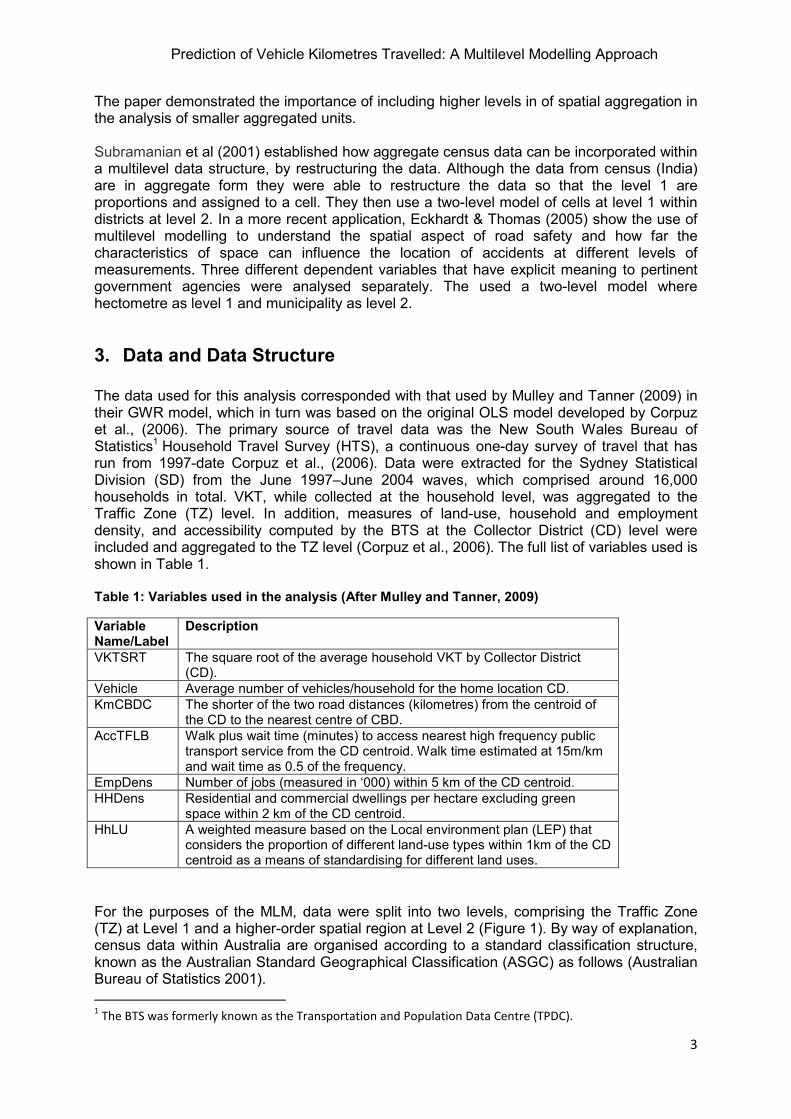
3. Data and Data Structure The data used for this analysis corresponded with that used by Mulley and Tanner (2009) in their GWR model, which in turn was based on the original OLS model developed by Corpuz et al., (2006). The primary source of travel data was the New South Wales Bureau of Statistics1 Household Travel Survey (HTS), a continuous one-day survey of travel that has run from 1997-date Corpuz et al., (2006). Data were extracted for the Sydney Statistical Division (SD) from the June 1997–June 2004 waves, which comprised around 16,000 households in total. VKT, while collected at the household level, was aggregated to the Traffic Zone (TZ) level. In addition, measures of land-use, household and employment density, and accessibility computed by the BTS at the Collector District (CD) level were included and aggregated to the TZ level (Corpuz et al., 2006). The full list of variables used is shown in Table 1. Table 1: Variables used in the analysis (After Mulley and Tanner, 2009)

Variable Name/Label

Description

VKTSRT The square root of the average household VKT by Collector District (CD).

Vehicle Average number of vehicles/household for the home location CD.

KmCBDC The shorter of the two road distances (kilometres) from the centroid of the CD to the nearest centre of CBD.

AccTFLB Walk plus wait time (minutes) to access nearest high frequency public transport service from the CD centroid. Walk time estimated at 15m/km and wait time as 0.5 of the frequency.

EmpDens Number of jobs (measured in ‘000) within 5 km of the CD centroid.

HHDens Residential and commercial dwellings per hectare excluding green space within 2 km of the CD centroid.

HhLU A weighted measure based on the Local environment plan (LEP) that considers the proportion of different land-use types within 1km of the CD centroid as a means of standardising for different land uses.

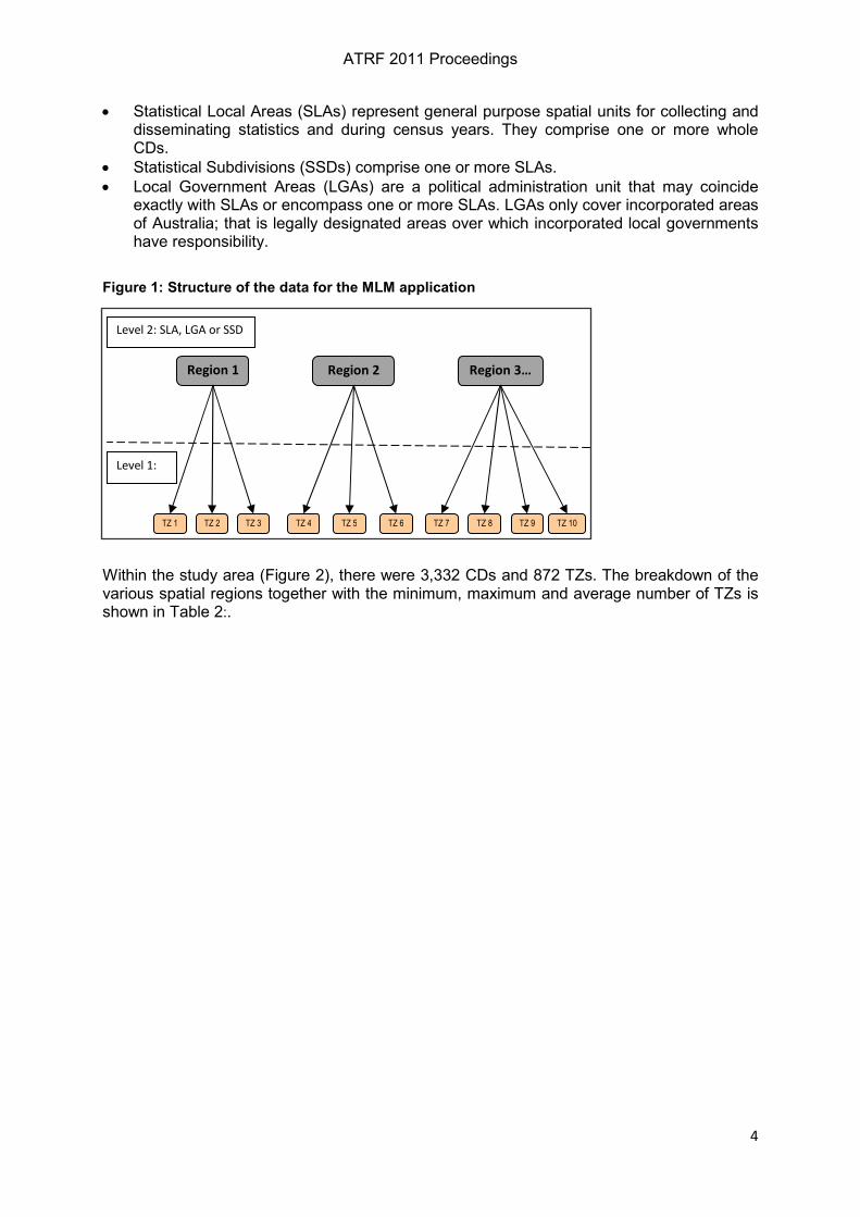
For the purposes of the MLM, data were split into two levels, comprising the Traffic Zone (TZ) at Level 1 and a higher-order spatial region at Level 2 (Figure 1). By way of explanation, census data within Australia are organised according to a standard classification structure, known as the Australian Standard Geographical Classification (ASGC) as follows (Australian Bureau of Statistics 2001).

1 The BTS was formerly known as the Transportation and Population Data Centre (TPDC).


4

• Statistical Local Areas (SLAs) represent general purpose spatial units for collecting and disseminating statistics and during census years. They comprise one or more whole CDs.

• Statistical Subdivisions (SSDs) comprise one or more SLAs.

• Local Government Areas (LGAs) are a political administration unit that may coincide exactly with SLAs or encompass one or more SLAs. LGAs only cover incorporated areas of Australia; that is legally designated areas over which incorporated local governments have responsibility.

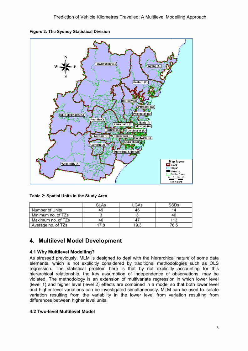
Within the study area (Figure 2), there were 3,332 CDs and 872 TZs. The breakdown of the various spatial regions together with the minimum, maximum and average number of TZs is shown in Table 2:.

Region 1

TZ 5

Region 3… Region 2

TZ 1 TZ 6 TZ 7 TZ 8 TZ 10 TZ 2 TZ 3 TZ 9 TZ 4

Level 2: SLA, LGA or SSD

Level 1:

TZ

Figure 1: Structure of the data for the MLM application


5

Figure 2: The Sydney Statistical Division

Table 2: Spatial Units in the Study Area

SLAs LGAs SSDs

Number of Units 49 46 14

Minimum no. of TZs 3 3 40

Maximum no. of TZs 40 47 113

Average no. of TZs 17.8 19.3 76.5

4. Multilevel Model Development 4.1 Why Multilevel Modelling?

As stressed previously, MLM is designed to deal with the hierarchical nature of some data elements, which is not explicitly considered by traditional methodologies such as OLS regression. The statistical problem here is that by not explicitly accounting for this hierarchical relationship, the key assumption of independence of observations, may be violated. The methodology is an extension of multivariate regression in which lower level (level 1) and higher level (level 2) effects are combined in a model so that both lower level and higher level variations can be investigated simultaneously. MLM can be used to isolate variation resulting from the variability in the lower level from variation resulting from differences between higher level units.

4.2 Two-level Multilevel Model


6

The traditional way of looking into the relationship between the two variables is to use ordinary regression of the form:

iii eXY ++= 10 ββ (1.1)

Where: iX (predictor/independent variable), iY (response/dependent variable), 0β (constant), 1β (slope), and ie (random error term).

For the case of a MLM with two levels of observations, namely i (level 1) grouped in a larger

region j (level 2), the response variable is now ijY . In this case, the regions are treated as a

random sample of the population regions, such that equation (1.1) can be expressed as follows:

ju+= ββ0

jijij uXY ++= 1ββ (1.2)

Here the β without a subscript is a constant, ijX represents the independent variables

across levels i and j, and ju represents the departures of the jth TZ intercept from the overall

value and also the level 2 residual, and ije represents the error across the lowest level (in this

case TZs). The model for actual VKT can now be expressed as:

ijjijij euXY +++= 1ββ . (1.3)

The means of ju and ije are equal to zero and are random quantities forming the random

part of the model described in (1.3). Since they are in different levels we can assume that these variables are uncorrelated and assumed to follow a normal distribution implying the

respective variances 2

uσ and 2

eσ can be estimated. The quantities β and 1β are the mean

intercept and slopes respectively and need to be estimated. The variances 2

uσ and 2

eσ are

considered as the random parameters, while β and 1β are considered the fixed parameters

of model (1.3). To be able to specify more general models we need to introduce a special explanatory

variable which takes the value 1 for all TZs and denote it with 0x . This will be used to allow

every term in the right hand side of equation (1.3) to be linked with an explanatory variable.

Now let us use the subscripted variables 0β , 1β , 2β … to denote the fixed parameters and

include a subscript 0 into the random variables as follows:

00100 xexuXxY ijjijij +++= ββ (1.4)

Rearranging equation (1.4) to ijijjij XxexuxY 10000 ββ +++= and letting ijjij eu ++= 00 ββ

allows us to specify the random variations in Y in terms of the random coefficient of the explanatory variables (Rasbash et al., 2001). Thus we have:

ijijij XxY 100 ββ +=

ijjij eu ++= 00 ββ


7

),(~ ΩXBNY

Here XB is the fixed part of the model and is a column vector while Ω is the variance/ covariance of the random terms for all levels of the data.

The Null Model The null model refers to a model where no independent variables are included. The null model describes the dependent variable as a function of an average value (the intercept) and is allowed to vary at random across the levels to look into the proportion of variation of the variance at the different levels. In the current situation this can be the mean VKT, the between-TZ variance and the between-LGA (or SLA or SSD) variance. The two-level null model can be described as:

ijjij euY ++= 0β (1.5)

2)var( uju σ= , 2)var( eije σ= .

The Variance Partition Coefficient (VPC) A convenient way of summarizing the importance of the level 2 (the regions) is the VPC defined as:

22

2

eu

uVPCσσ

σ

+= (1.6)

Aside from summarizing the importance of the regions, the VPC can also indicate the residual correlation between the VKTs from two TZs in the same region. Estimation of Parameters For the purpose of this analysis, the special-purpose multilevel modelling software, Mlwin was used (Rasbash et al., 2009). It has a graphical user interface for specification and fitting of wide range of multilevel models. It uses several estimation methods that include maximum likelihood and Markov Chain Monte Carlo (MCMC). For this analysis, the approximation of parameters was done using Iterative Generalised Least Squares (IGLS). 5. RESULTS Appropriateness of MLM The first step was to establish if it was statistically valid to use MLM, particularly given the aggregated nature of the VKT data. Tests of heteroscedasticity on the VKT (aggregated at TZ level) using visual tests conducted in SPSS and White’s test resulted in verifying the data were not heteroscedastic, confirming that a MLM approach could be used. The second issue was to establish the appropriateness of MLM for the analysis of the present data by examining the proportion of unexplained variance at each level. This is done by examining the different null models below. The Null Models

Null models (i.e., those with no independent variables) were estimated for the three different Level 2 scenarios, namely LGAs, SLAs and SSDs. The proportion of variation attributable to the different levels was estimated using the definitional formula in equations 1.5 and 1.6 and results are shown in Table 3. By way of interpretation, the Level 1 variance represents the variance in the VKT (square-root) across the 872 TZs, while the Level 2 variance represents the variance in the VKT (square-root) across the 49 LGAs, 46 SLAs, and 14 SSDs


8

respectively. The VPC (variance partition coefficient) indicates the proportion of the total variance in VKT that is attributed to the Level 2 groupings, which in this case is 51.8% (when LGAs are used at Level 2), 54.3% (SLAs), and 43.7% (SSDs). Evidently, a large proportion of the variance in VKT is explicable by the hierarchical nature of the data, suggesting that MLM is a potentially useful and valid approach. Table 3: Variance Estimates and VPCs for the Null Models

Level 2 Structure

Null Model LGA SLA SSD

Level 2 variance 3.08 3.331 2.616

Level 1 variance 2.870 2.802 3.367

VPC 0.518 0.543 0.437

Univariate Models Univariate models were developed in which each of the variables identified in Table 1 were introduced separately. In effect this involves fitting parallel lines, corresponding to the number of Level 2 spatial units, to establish the directionality of the relationship and the difference in mean effects between them. As expected the relationships with VKT are positive for vehicles, KmCBDC, and AccTFLB and negative for HhLU, HHDens and EmpDens. Full Models

The full models involved introducing all the independent variables at Level 1, resulting in a multivariate MLM. Table 4 indicates the variance attributable to the different levels and the VPC. Using LGAs as an example, the level 2 variance of VKT (square-root) is now 0.218, a reduction of 92.9%, while 12 percent of the variation is now attributed to the level 2 groupings, a reduction of 69.5%. Clearly, the introduction of the independent variables has reduced the unexplained variance in VKT substantially at both levels, suggesting that (perhaps not surprisingly) the impacts are felt both at the TZ and regional level. Table 4: Variance Estimates and VPCs for the Full Models

Level 2 Structure

LGA SLA SSD

Level 2 variance 0.218 (92.9%) 0.209 (93.7%) 0.271 (89.6%)

Level 1 variance 1.599 (44.3%) 1.595 (43.1%) 1.661 (52.1%)

VPC 0.120 (69.5%) 0.116 (70.6%) 0.140 (68.5%)

*Variance reduction compared to the null model shown in parentheses

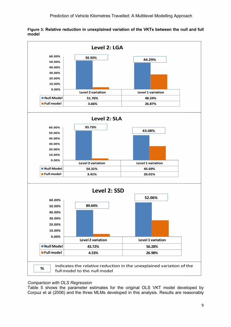
It is also useful to visualise the reduction rate of variation in the full model relative to that of the null model (Figure 3). By way of interpretation, taking the case of LGAs, the unexplained variance at Level 2 has decreased from 51.76% to 3.66%, while the Level 1 variation has decreased from 48.24% to 26.87% for the full model. This reinforces the finding that entry of the level 1 variables has in fact had a more dramatic effect on the reduction in level 2 variance.


9

Figure 3: Relative reduction in unexplained variation of the VKTs between the null and full model

Comparison with OLS Regression Table 5 shows the parameter estimates for the original OLS VKT model developed by Corpuz et al (2006) and the three MLMs developed in this analysis. Results are reasonably

Level 2 variation Level 1 variation

Null Model 51.76% 48.24%

Full model 3.66% 26.87%

0.00%

10.00%

20.00%

30.00%

40.00%

50.00%

60.00%

Level 2: LGA

92.92%44.29%


Null Model 54.31% 45.69%

Full model 3.41% 26.01%

0.00%

10.00%

20.00%

30.00%

40.00%

50.00%

60.00%

Level 2: SLA

93.73%43.08%


Null Model 43.72% 56.28%

Full model 4.53% 26.98%

0.00%

10.00%

20.00%

30.00%

40.00%

50.00%

60.00%

Level 2: SSD

89.64%

52.06%

%indicates the relative reduction in the unexplained variation of the

full model to the null model


10

similar for the SLA and LGA groupings except for the distance to CBD or major centre (KmCBDC), which was borderline significant using the OLS Method but not significant for the MLMs. For the more aggregate grouping, SSDs, the main difference is that employment density (EmpsDens) is now not significant. Table 5: Comparison of OLS and Multilevel Models

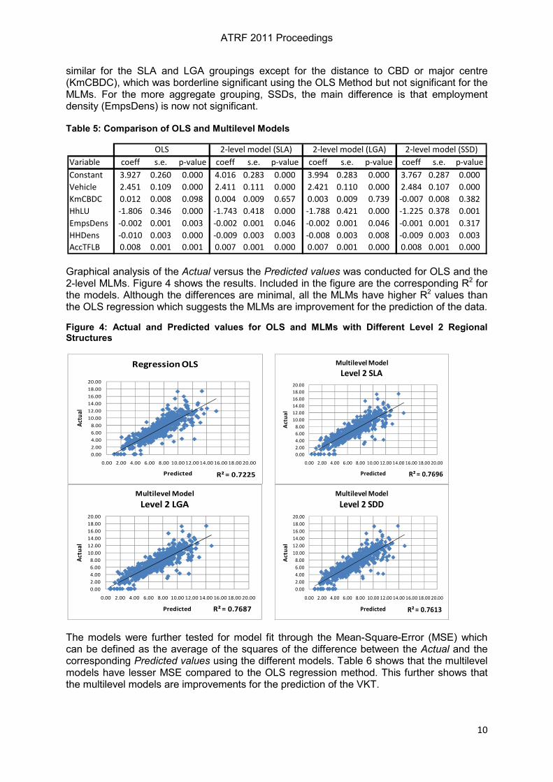
Graphical analysis of the Actual versus the Predicted values was conducted for OLS and the 2-level MLMs. Figure 4 shows the results. Included in the figure are the corresponding R2 for the models. Although the differences are minimal, all the MLMs have higher R2 values than the OLS regression which suggests the MLMs are improvement for the prediction of the data.

Figure 4: Actual and Predicted values for OLS and MLMs with Different Level 2 Regional Structures

The models were further tested for model fit through the Mean-Square-Error (MSE) which can be defined as the average of the squares of the difference between the Actual and the corresponding Predicted values using the different models. Table 6 shows that the multilevel models have lesser MSE compared to the OLS regression method. This further shows that the multilevel models are improvements for the prediction of the VKT.

Variable coeff s.e. p-value coeff s.e. p-value coeff s.e. p-value coeff s.e. p-value

Constant 3.927 0.260 0.000 4.016 0.283 0.000 3.994 0.283 0.000 3.767 0.287 0.000

Vehicle 2.451 0.109 0.000 2.411 0.111 0.000 2.421 0.110 0.000 2.484 0.107 0.000

KmCBDC 0.012 0.008 0.098 0.004 0.009 0.657 0.003 0.009 0.739 -0.007 0.008 0.382

HhLU -1.806 0.346 0.000 -1.743 0.418 0.000 -1.788 0.421 0.000 -1.225 0.378 0.001

EmpsDens -0.002 0.001 0.003 -0.002 0.001 0.046 -0.002 0.001 0.046 -0.001 0.001 0.317

HHDens -0.010 0.003 0.000 -0.009 0.003 0.003 -0.008 0.003 0.008 -0.009 0.003 0.003

AccTFLB 0.008 0.001 0.001 0.007 0.001 0.000 0.007 0.001 0.000 0.008 0.001 0.000

OLS 2-level model (SLA) 2-level model (LGA) 2-level model (SSD)

R² = 0.7225

0.00

2.00

4.00

6.00

8.00

10.00

12.00

14.00

16.00

18.00

20.00

0.00 2.00 4.00 6.00 8.00 10.00 12.00 14.00 16.00 18.00 20.00

Act

ual

Predicted

Regression OLS

R² = 0.7696

0.00

2.00

4.00

6.00

8.00

10.00

12.00

14.00

16.00

18.00

20.00

0.00 2.00 4.00 6.00 8.00 10.00 12.00 14.00 16.00 18.00 20.00

Act

ua

l

Predicted

Multilevel Model

Level 2 SLA

R² = 0.7687

0.00

2.00

4.00

6.00

8.00

10.00

12.00

14.00

16.00

18.00

20.00

0.00 2.00 4.00 6.00 8.00 10.00 12.00 14.00 16.00 18.00 20.00

Act

ua

l

Predicted

Multilevel Model

Level 2 LGA

R² = 0.7613

0.00

2.00

4.00

6.00

8.00

10.00

12.00

14.00

16.00

18.00

20.00

0.00 2.00 4.00 6.00 8.00 10.00 12.00 14.00 16.00 18.00 20.00

Actu

al

Predicted

Multilevel Model

Level 2 SDD


11

Table 6: Mean-Square-Error Estimates for the Different Models

6. Conclusions The premise behind this paper is that VKT is influenced by land-use/accessibility/density factors that operate at a ‘higher’ level. While data constraints imposed the necessity of working at the TZ level, which in itself is an aggregate entity, the paper never-the-less demonstrated the following. First, the estimates of the VPCs for the null models suggested around half the variation in VKT was due to the upper level being considered (SLA, LGA and SSD). Second, the introduction of the independent level 1 variables reduced the unexplained variance in VKT substantially at both levels, which was in line with intuition. Third, diagnostics of model fit suggested the MLMs offered improvements over current OLS methods. While MLM has a certain intrinsic appeal, it does come with caveats. First, is that the actual application of MLM is significantly more complex than conventional regression-based techniques and particular care has to be taken in how the data are organised and levels defined. Second, interpretation can be challenging and is again often heavily influenced by how exactly the data are set up. Third, is a more specific issue with the analysis here, which relates to the use of an aggregate unit as the basic building block (level 1). Although this has been done before, logic suggests that it would be preferable to treat the household as the level 1 entity with the spatial effects operating at levels 2. This is the focus of current work using the Sydney HTS.

7. References Australian Bureau of Statistics 2001, Australian Standard Geographical Classifications (ASCG). Catalogue No.1216.0 2001.

Chikaraishi, M., A. Fujiwara, J. Zhang and K.W. Axhausen. Exploring Variation Properties of Departure Time Choice Behavior by Using Multilevel Analysis Approach. In Transportation Research Record: Journal of the Transportation Research Board, No. 2134, Transportation Research Board of the National Academies, Washington, D.C., 2009, pp. 10-20.

Congdon, P., (1997) Multilevel and clustering analysis of health outcomes in small areas. European Journal of Populations 13, pp. 305–338.

Corpuz, G, McCabe, M and Ryszawa, K.(2006), The Development of a Sydney VKT Regression Model, 32nd Australasian Transport Research Forum.

Dupont, E. and H. Martensen (Eds.). Multilevel modelling and time series analysis in traffic research – Methodology. Deliverable D7.4 of the EU FP6 project SafetyNet., 2007.

Eckhardt Nathalie, Thomas Isabelle, Spatial nested Scales for Road Accidents in the Periphery of Brussels, IATSS Research, 29, 1, 2005, p. 66-78.

Familar, R., Greaves, S.P., Ellison, A.B. Analysing speeding behaviour: A multilevel modelling approach. Working Paper ITLS-WP-11-05 (2011)

Jones, K. and Duncan, C. People and Places: The multilevel model as a general framework for the quantitative analysis of geographical data. In Longley, P and Batty, M (Eds.),Spatial Analysis: Modelling in a GIS Environment : Pearson Professional Ltd., UK,(1996), p. 79-104.

Model OLS MLM SLA MLM LGA MLM SSD

MSE 2.076 1.535 1.539 1.590


12

Langford, I. H. and Bentham, G. (1996). ‘Regional variations in mortality rates in England and Wales: an analysis using multilevel modelling’, Social Science and Medicine, 42.6, 897Ð908.

Langford I H, Bentham G, McDonald A-L, 1998, ``Multilevel modelling of geographically aggregated health data: a case study on malignant melanoma mortality and UV exposure in the European community'' Statistics in Medicine 17 41-57.

Mulley and Tanner (2009). The Vehicle Kilometres ravelled (VKT) by Private Car: A Spatially Analysis Using Geographically Weighted Regression. Australasian Transport Research Forum, Auckland New Zealand. Tanner

Rasbash, JR & Browne, WJ. 'Modelling non-hierarchical structures', in A.H. Leyland and H Goldstein (Eds.), Multilevel modelling of health statistics, (pp. 93-105), Chichester: John Wiley and Sons, 2001. ISBN: 0471998907.

Subramanian, S. V., Duncan, C., et al. (2001). Multilevel perspectives on modeling census data. Environment and Planning A 33(3): 399-417.

Documents

Prediction of Vehicle Kilometres Travelled: A Multilevel ...€¦ · effects at a particular level may reflect many influences that operate at that level such as physical features,