EPA 905/R-00/007 June 2000

Prediction of sediment toxicity usingconsensus-based freshwater sediment quality guidelines

United States Geological Survey (USGS) final report forthe U.S. Environmental Protection Agency (USEPA)

Great Lakes National Program Office (GLNPO)

Christopher G Ingersoll1, Donald D MacDonald2, Ning Wang3,Judy L Crane4, L Jay Field5, Pam S Haverland1, Nile E Kemble1,Rebekka A Lindskoog2, Corinne Severn6, and Dawn E Smorong2

1Columbia Environmental Research Center, USGS4200 New Haven Road, Columbia, MO 65201

2MacDonald Environmental Sciences Limited,2376 Yellow Point Road, Nanaimo, British Columbia, Canada V9X 1W5

3Fisheries and Wildlife Sciences, 302 ABRN Building,University of Missouri, Columbia, MO 65211

4Minnesota Pollution Control Agency, 520 Lafayette Rd., St. Paul, MN 55155

5National Oceanic and Atmospheric Administration (NOAA), 7600 Sand Point Way NE, Seattle, WA 98115

6EVS Environment Consultants, 200 West Mercer Street, Seattle, WA 98119

Project Officer: Marc TuchmanUSEPA GLNPO77 West Jackson

Chicago, IL 60604

Abstract

The primary objectives of this study were to: (1) evaluate the ability of consensus-based SQGs (sediment quality guidelines) to predict toxicity in a freshwater database for field-collected sediments in the Great Lakes basin; (2) evaluate the ability of SQGs to predict sediment toxicity on a regional geographic basis elsewhere in North America; and (3) compare approaches for evaluating the combined effects of chemical mixtures on the toxicity of field-collected sediments. A database was developed from 92 published reports which included a total of 1657 samples with high-quality matching sediment toxicity and chemistry data. The database was comprised primarily of 10- to 14-day or 28- to 42-day toxicity tests with the amphipod Hyalella azteca (designated as the HA10 or HA28 tests) and 10- to 14-day toxicity tests with the midges Chironomus tentans or C. riparius (designated as the CS10 test). Endpoints reported in these tests were primarily survival or growth. Because field-collected sediments typically contain complex mixtures of contaminants, the predictive ability of a sediment assessment is likely to increase when SQGs are used in combination to classify toxicity of sediments. For this reason, the evaluation of the predictive ability of probable effect concentrations (PECs) was conducted to determine the incidence of effects above and below various mean PEC quotients (mean quotients of 0.1, 0.5, 1.0, and 5.0). The PECs are SQGs that were established as concentrations of individual chemicals above which adverse effects in sediments are expected to frequently occur. A PEC quotient was calculated for each chemical in each sample in the database by dividing the concentration of a chemical by the PEC for that chemical. A mean quotient was calculated for each sample by summing the individual quotient for each chemical and then dividing this sum by the number of PECs evaluated.

When mean quotients were calculated using an approach of equally weighting up to 10 reliable PECs (PECs for metals, total polycyclic aromatic hydrocarbons (PAHs), total polychlorinated biphenyls (PCBs), and sum DDE), there was an overall increase in the incidence of toxicity with an increase in the mean quotient in all three tests. For example in the HA10 test, the toxicity of samples was 20% at mean quotients of <0.1 and increased to 67% at mean quotients of >5.0. Similarly, for the CS10 test there was a 20% incidence of toxicity at mean quotients of <0.1 increasing to a 64% incidence of toxicity at mean quotients of >5.0. In contrast, the incidence of toxicity in the HA28 test was only 8% at mean quotients of <0.1 and increased to 91% at mean quotients of >1.0. In all three tests, there was a consistent increase in the toxicity at mean quotients of >0.5. However, the overall incidence of toxicity was greater in the HA28 test compared to the short-term tests.

The incidence of toxicity at mean quotients of <0.1 was somewhat higher in the HA10 and CS10 tests (20%) compared to the HA28 test (8%). This toxicity at low mean quotients does not appear to be related to total organic carbon in sediment. There was insufficient information in the database to evaluate effects of grain size on toxicity. Unmeasured contaminants in these field-collected sediments or contaminants for which we do not have reliable PECs (i.e., pesticides, herbicides) may have contributed to this toxicity at low mean quotients. Alternatively, the data for HA10 and CS10 tests were obtained from numerous laboratories which may have contributed to variability in the data reported in these studies. In contrast, a limited number of laboratories conducted most of the HA28 tests.

The reason for the higher incidence of toxicity with increasing mean quotients in the HA28 test compared to the short-term tests may be due to the duration of the exposure or the sensitivity of

2

growth in the longer HA28 test. A 50% incidence of toxicity in the HA28 test corresponds to a mean quotient of 0.63 when survival or growth were used to classify a sample as toxic. By comparison, a 50% incidence of toxicity is expected at a mean quotient of 3.2 when survival alone was used to classify a sample as toxic in the HA28 test. In the CS10 test, a 50% incidence of toxicity is expected at a mean quotient of 9.0 when survival alone was used to classify a sample as toxic or at a mean quotient of 3.5 when survival or growth were used to classify a sample as toxic. In contrast, similar mean quotients resulted in a 50% incidence of toxicity in the HA10 test when survival alone (mean quotient of 4.5) or when survival or growth (mean quotient of 3.4) were used to classify a sample as toxic. Results of these analyses indicate that both the duration of the exposure and the endpoints measured can influence whether a sample is found to be toxic or not. The longer-term tests in which growth and survival are measured tended to be more sensitive than shorter-term tests, with acute to chronic ratios on the order of 6 indicated for H. azteca.

We were also interested in determining the predictive ability of PEC quotients for major classes of compounds. Therefore, we evaluated the incidence of toxicity based on a mean quotient for metals, a quotient for total PAHs, or a quotient for total PCBs. Different patterns of toxicity associated with the various procedures for calculating quotients were observed. For example in the HA28 test, a relatively abrupt increase in toxicity was associated with elevated PCBs alone or with elevated PAHs alone, compared to the pattern of a gradual increase in toxicity observed with quotients calculated using a combination of metals, PAHs, and PCBs. These analyses indicate that the different patterns in toxicity may be the result of unique chemical signals associated with individual contaminants. While mean quotients can be used to classify samples as toxic or non-toxic, individual quotients might be useful in helping to identify substances that may be causing or substantially contributing to the observed toxicity.

We chose to make comparisons across geographic areas using mean quotients calculated by equally weighting the contribution of the three major classes of compounds (metals, or PAHs, or PCBs). This approach assumes that these three diverse groups of chemicals exert some form of joint toxic action. Use of this approach also maximized the number of samples that were used to make comparisons across geographic areas. Generally, there was an increase in the incidence of toxicity with increasing mean PEC quotients within most of the regions, basins, and areas for all three toxicity tests. For the HA10 and HA28 tests, the incidence of toxicity for samples from each of the Great Lakes and within the areas of each Great Lake was relatively consistent with the overall pattern of toxicity in the entire database. However, the relationship between the incidence in toxicity and mean quotients in the CS10 test was more variable among geographic areas compared to either the HA10 or HA28 test. The results of these analyses indicate that the consensus-based PECs can be used to reliably predict toxicity of sediments on both a regional and national basis.

This paper presents results of the first analyses completed on the entire freshwater sediment database. Some of the additional analyses planned for the database that are beyond the scope of this paper include: (1) comparing approaches for designating samples as toxic; (2) evaluating logistic-regression models; (3) identifying a list of optimal analytes for broad scale application and testing the relative efficacy of the mean versus the sum PEC quotients; (4) evaluating the influence of grain size and ammonia on the incidence of toxicity; and (5) developing a guidance manual for conducting an integrated assessment of sediment contamination.

3

Contents

Abstract ........................................................................................................................................... 2 List of Figures ................................................................................................................................. 4 List of Tables................................................................................................................................... 4 List of Appendices........................................................................................................................... 4 Acknowledgments ........................................................................................................................... 5 Introduction ..................................................................................................................................... 6 Methods........................................................................................................................................... 7 Results and Discussion.................................................................................................................. 11 Summary ....................................................................................................................................... 21 References ..................................................................................................................................... 23 Figures ........................................................................................................................................... 26 Tables ............................................................................................................................................ 28 Appendices .................................................................................................................................... 33

List of Figures

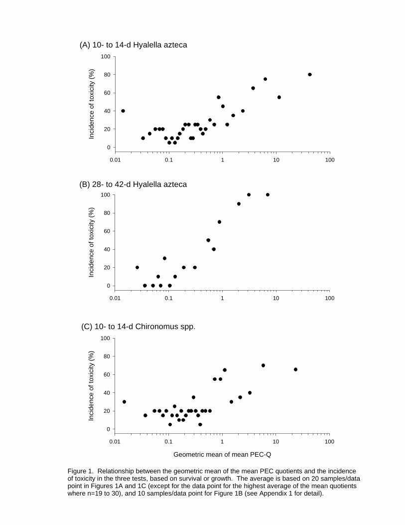
Figure 1. Relationship between the geometric mean of the mean PEC quotients and the incidence of toxicity in the three tests, based on survival or growth.

Figure 2. Relationship between the geometric mean of the mean PEC quotients and the incidence of toxicity in the three tests, based on survival or growth, or based on survival alone.

List of Tables

Table 1. Sediment quality guidelines that reflect probable effect concentrations.

Table 2. Incidence of sediment toxicity within ranges of PEC quotients (calculated using various approaches) for freshwater tests based on survival or growth.

Table 3. Incidence of sediment toxicity within ranges of PEC quotients for the Hyalella azteca 10- to 14-day test in various geographic areas within the database based on survival or growth.

Table 4. Incidence of sediment toxicity within ranges of PEC quotients for the Hyalella azteca 28- to 42-day test in various geographic areas within the database based on survival or growth.

Table 5. Incidence of sediment toxicity within ranges of PEC quotients for the Chironomus spp. 10- to 14-day test in various geographic areas within the database based on survival or growth.

List of Appendices

Appendix 1. Summary of the data presented in Figures 1 and 2.

4

Acknowledgments

We thank the members of the Sediment Advisory Group on Sediment Quality Assessment for insight and guidance in developing the procedures for evaluating the predictive ability of freshwater sediment quality guidelines. We would also like to thank Kathie Adare, Peter Landrum, and Rick Swartz for providing helpful review comments on the report. Although information in this report was developed in part by the USGS, USEPA, and NOAA, the report may not necessarily reflect the reviews of these organizations and no official endorsement should be inferred. Sediment quality guidelines (SQGs) can be used as one of several tools to assess contaminated sediments; however, there is no intent expressed or implied that these guidelines represent USGS, USEPA, or NOAA sediment quality criteria. Information in this report and the development of the database have been funded in part by the USEPA Great Lakes National Program Office, USEPA Office of Research and Development, USEPA Office of Water, Minnesota Pollution Control Agency, and National Research Council of Canada. This report has been reviewed in accordance with USEPA and USGS policy.

5

Introduction

Numerical sediment quality guidelines (SQGs) have been developed by a variety of federal, state, and provincial agencies across North America using matching sediment chemistry and biological effects data. These SQGs have been routinely used to interpret historical data, identify potential problem chemicals or areas at a site, design monitoring programs, classify hot spots and rank sites, and make decisions for more detailed studies (Long and MacDonald 1998). Additional suggested uses for SQGs include identifying the need for source controls of problem chemicals before release, linking chemical sources to sediment contamination, triggering regulatory action, and establishing target remediation objectives (USEPA 1997). Numerical SQGs, when used with other tools such as sediment toxicity tests, bioaccumulation, and benthic community surveys, can provide a powerful weight of evidence for assessing the hazards associated with contaminated sediments (Ingersoll et al. 1997).

A critical component in the application of SQGs for assessing sediment quality is a demonstration of the ability of the guidelines to predict the absence or presence of toxicity in field-collected sediments (Ingersoll et al. 1996, Smith et al. 1996, Long et al. 1998a, Swartz 1999, Fairey et al. 2000, MacDonald et al. 2000a,b). This paper is the fourth in a series that is intended to address the ability of various SQGs to predict toxicity in contaminated sediments. The first paper in the series focused on resolving the “mixture paradox” that is associated with the application of empirically-derived SQGs for individual polycyclic aromatic hydrocarbons (PAHs). In this case, the paradox was addressed by developing consensus-based SQGs for total PAHs (Swartz 1999). A second paper developed and evaluated consensus-based SQGs for total polychlorinated biphenyls (PCBs) to address a similar mixture paradox for that group of contaminants (MacDonald et al. 2000b).

A third paper developed consensus-based SQGs for freshwater sediments (MacDonald et al. 2000a). The published SQGs for 28 chemical substances were assembled and classified into two categories in accordance with their original narrative intent. These published SQGs were then used to develop two consensus-based SQGs for each contaminant, including a threshold effect concentration (TEC; below which adverse effects are not expected to occur) and a probable effect concentration (PEC; above which adverse effects are expected to frequently occur; Table 1; MacDonald et al. 2000a). A preliminary evaluation of the predictive ability of these consensus-based SQGs for freshwater sediment was conducted using a database of 347 samples obtained from 15 separate studies. The results of these three previous investigations demonstrated that the consensus-based SQGs provide a unifying synthesis of the existing guidelines, reflect causal rather than correlative effects, and account for the effects of contaminant mixtures in sediment (Swartz 1999, MacDonald et al. 2000a,b).

The primary objective of this fourth paper is to further evaluate the predictive ability of the consensus-based PECs developed by MacDonald et al. (2000a). The database used by MacDonald et al. (2000a) was expanded to include a total of 1657 samples from 92 published reports with high-quality matching sediment toxicity and chemistry data. The majority of the data from these reports were for 10- to 28-day toxicity tests with the amphipod Hyalella azteca or 10-to 14-day toxicity tests with the midges Chironomus tentans or C. riparius. The endpoints

6

measured in these toxicity tests primarily included survival or growth of test organisms at the end of the sediment exposures. A second objective of this paper is to evaluate the predictive ability of these PECs on a regional basis within the larger database. We were interested in determining if there are differences in the predictive ability of the PECs across the entire database compared to various geographic areas within the database, such as all of the samples from the Great Lakes or all of the samples from an area within a Great Lake, such as Indiana Harbor or Waukegan Harbor located within Lake Michigan.

Methods

Development of consensus-based sediment quality guidelines

Individual SQGs for freshwater ecosystems have previously been developed using a variety of approaches (Table 1). Each of these approaches has certain advantages and limitations which influence their application in the sediment quality assessment process (Ingersoll et al. 1997). In an effort to focus on the agreement among these various published SQGs, consensus-based SQGs were developed by MacDonald et al. (2000a) for 28 chemicals of concern in freshwater sediments (i.e., metals, PAHs, PCBs, and pesticides). For each contaminant of concern, two consensus-based SQGs were developed from published SQGs, including a threshold effect concentration (TEC) and a probable effect concentration (PEC). The TECs were calculated by determining the geometric mean of the SQGs that were included in this category (MacDonald et al. 2000a). Likewise, consensus-based PECs were calculated by determining the geometric mean of the PEC-type values (Table 1). The geometric mean, rather than the arithmetic mean or median, was calculated because it provides an estimate of central tendency that is not unduly affected by extreme values and because the distributions of the SQGs were not known (MacDonald et al. 2000a). Consensus-based TECs or PECs were calculated only if three of more published SQGs were available for a chemical substance or group of substances. The evaluations of toxicity in the present study were based on the use of PECs because TECs were developed to provide an estimate of conditions where toxicity would not be expected and PECs were developed to provide an estimate of conditions where toxicity would be expected. Evaluations of SQGs in the present study were based on dry-weight concentrations because previous studies have demonstrated that normalization of SQGs for PAHs or PCBs to total organic carbon (Barrick et al. 1988, Long et al. 1995, Ingersoll et al. 1996) or normalization of metals to acid-volatile sulfides (Long et al. 1998b) did not improve the predictions of toxicity in field-collected sediments.

The consensus-based PECs listed in Table 1 were critically evaluated by MacDonald et al. (2000a) to determine if they would provide effective tools for assessing sediment quality conditions in freshwater ecosystems. The criteria for evaluating the reliability of the consensus-based PECs were adapted from Long et al. (1998a). Specifically, the individual TECs were considered to provide a reliable basis for assessing the quality of freshwater sediments if >75% of the sediment samples were correctly predicted to be not toxic. Similarly, the individual PEC for each substance was considered to be reliable if >75% of the sediment samples were correctly predicted to be toxic using the PEC. Therefore, the target levels of both false positives (i.e., samples incorrectly classified as toxic) and false negatives (i.e., samples incorrectly classified as

7

not toxic) was 25% using the TEC and PEC. To assure that the results of this evaluation were not unduly influenced by the number of sediment samples, the various SQGs were considered to be reliable only if a minimum of 20 samples were included in the evaluation (i.e., 20 samples above at a PEC or 20 samples below a TEC; CCME 1995). The results of this evaluation described in MacDonald et al. (2000a) indicated that most of the TECs (i.e., 21 of 28) provide an accurate basis for predicting the absence of sediment toxicity. Similarly, most of the PECs (i.e., 16 of 28) provide an accurate basis for predicting sediment toxicity (Table 1).

A reliable TEC or PEC was not available for mercury, an important contaminant of concern in sediments (Table 1). This lack of reliability is most likely due to the speciation of mercury in the sediments, as well as the ability of methyl mercury to bioaccumulate in organisms. Sediment quality guidelines developed using a tissue residue approach are needed to establish safe sediment concentrations for human health and piscivorus-wildlife receptors (Ingersoll et al. 1997). For this report, only direct toxic effects on benthic invertebrates are considered in the evaluation of the predictability of the consensus-based SQGs.

Development of the sediment toxicity database

To support the development of the sediment toxicity database, matching sediment chemistry and biological effects data were compiled for various freshwater locations across North America (in addition to the data that were used in the analyses performed by MacDonald et al. 2000a). Candidate data sets were identified by reviewing the published literature and by contacting individuals active in the field of sediment quality assessment. More than 1500 documents were reviewed and evaluated to obtain the data required to evaluate SQGs in the present study. Because these data sets were generated for a wide variety of purposes, each study was critically-evaluated to assure the quality of the data used for evaluating the predictive ability of the SQGs (Long et al. 1998a, Ingersoll and MacDonald 1999). Data from individual studies were considered acceptable for use in the present study if:

• The study was conducted in a freshwater location in North America; • Appropriate procedures were used to collect, handle, and store sediments (e.g., ASTM

2000, USEPA 2000); • Matching sediment chemistry and biological effects data were reported and

concentrations of contaminants were measured in each sample or treatment group. • Minimum data quality requirements were reported. For example, analytical detection

limits were lower than freshwater probable effect levels (PEL; Smith et al. 1996), accuracy and precision were within acceptable limits, and analytes were not present at detectable levels in method blanks;

• Appropriate analytical methods were used to generate chemistry data. For metals, concentrations of total metals needed to be reported. However, other measures of metal concentrations were used (i.e., simultaneously extracted metals) if sufficient information was available to demonstrate that these measures are comparable to total metal concentrations (Ingersoll et al. 1996, 1998). For organic compounds, the concentrations needed to be measured using gas chromatography-mass spectroscopy, high pressure liquid chromatography, or comparable methods; and,

8

• Toxicity tests needed to meet test acceptability criteria outlined in ASTM (2000) and USEPA (2000) and endpoints measured needed to be ecologically relevant (likely to influence the viability of the organism in the field) or needed to be indicative of ecologically-relevant endpoints.

Using these selection criteria, a total of 92 freshwater data sets were incorporated into a database that included 1657 individual sediment samples. The toxicity tests in this database primarily include tests with the amphipod, Hyalella azteca; the midges, Chironomus tentans or C. riparius; the mayfly, Hexagenia limbata; the oligochaete, Lumbriculus variegatus; the daphnids, Ceriodaphnia dubia or Daphnia magna; and, the bacterium, Vibrio fisheri (Microtox). We selected a subset of the samples from this database that reported sediment chemistry for at least one of the substances for which reliable SQGs were listed in Table 1. We then selected a subset of these resultant samples with matching toxicity data for the amphipod Hyalella azteca or the midges Chironomus tentans or C. riparius. Tests with H. azteca and Chironomus spp. were selected because the samples that were tested represented a broader geographic area compared to the other tests in the database. The selected studies provided 670 samples for H. azteca 10- to 14-day tests (designated as HA10), 160 samples for H. azteca 28- to 42-day tests (designated as HA28) and 632 samples for Chironomus spp. 10- to 14-day tests (CS10; 556 of the samples were for tests with C. tentans and 76 of the samples were for tests with C. riparius). We combined the data for the two midge species due to the limited amount of data for C. riparius. Preliminary analyses of the database indicated similar sensitivity for these two species of midge. The selected studies represented a broad range in both sediment toxicity and contamination. A total of 28% of the samples were toxic in the HA10 test, 35% of the samples were toxic in the HA28 test, and 27% of the samples were toxic in the CS10 test (28% of the samples were toxic in the C. tentans tests and 21% of the samples were toxic in the C. riparius tests). Toxicity of samples was determined as a significant reduction in survival or growth relative to a control or reference sediment (as designated in the original study or determined using appropriate statistical procedures). Sexual maturation and reproduction were periodically reported in the HA28 test; however, these two additional endpoints did not identify any additional samples as toxic relative to effects reported on survival or growth of amphipods.

The total PCB concentration in each sediment sample in the database was calculated by summing dry-weight concentrations of individual congeners. If only aroclors concentrations were reported, total PCBs were calculated as the sum concentration of all individual aroclors. If both congeners and aroclors were reported, the congeners were used to calculate the concentration total PCBs in a sample. If only total PCBs was reported for a sample, then this value was used. The total PAH concentration in each sediment sample was generally calculated by summing the dry-weight concentrations from as many of the following 13 compounds that were reported: acenaphthene, acenaphthylene, anthracene, fluorene, 2-methylnaphthalene, naphthalene, phenanthrene, benz(a)anthracene, dibenz(a,h)anthracene, benzo(a)pyrene, chrysene, fluoranthene, and pyrene. Total PAHs were calculated using eight or less of these individual PAHs for <5% of the samples in the database. In calculating total PCBs or total PAHs, half the detection limit was used for compounds reported below the detection limit. Similarly, half of the detection limit was used for concentrations of metals below the detection limit. For DDTs, the concentrations of p,p’-DDD and o,p’-DDD, p,p’-DDE and o,p’-DDE, and p,p’-DDT and o,p’-DDT were summed to calculate

9

the concentrations of sum DDD, sum DDE, and, sum DDT, respectively. Total DDT was calculated by summing the concentrations of sum DDD, sum DDE, and, sum DDT. If all individual PCBs, PAHs, DDD, DDE, or DDT were less that the detection limit, the detection limits were summed and reported as a less than value for the sum.

Analysis of data

The initial evaluation of predictive ability by MacDonald et al. (2000a) focused primarily on determining the ability of each SQG, when applied alone, to correctly classify samples as toxic or not toxic. Because field-collected sediments typically contain complex mixtures of contaminants, the predictive ability of these sediment quality assessment tools is likely to increase when the SQGs are used in combination to classify toxicity of sediments. For this reason, the evaluation of the predictive ability of the SQGs in the present study was conducted to determine the incidence of effects above and below various mean PEC quotients (mean quotients of 0.1, 0.5, 1.0, and 5.0; Ingersoll et al. 1998, Long et al. 1998a, Fairey et al. 2000).

A PEC quotient was calculated for each chemical in each sample in the database by dividing the concentration of a chemical by the PEC for that chemical. A mean quotient was then calculated for each sample by summing the individual quotient for each chemical and dividing this sum by the number of reliable PECs evaluated. MacDonald et al. (2000a) found that some PEC values were more reliable predictors of toxicity and that use of only these PECs reduced the variability in the prediction of sediment toxicity compared to using all available PECs. The PEC for total PAHs, instead of the PECs for the individual PAHs, was used in the calculation to avoid double accounting of the PAH data (MacDonald et al. 2000a). This resulted in the use of up to 10 reliable PECs in calculating the mean quotient (arsenic, cadmium, chromium, copper, lead, nickel, zinc, total PAHs, total PCBs, and sum DDE; Table1 and designated “Mean - all” in Table 2). This approach to the calculation of mean quotients weighs each of the chemicals and chemical classes equally (Ingersoll et al. 1998, Long et al. 1998a, MacDonald et al. 2000a).

In the present study, a second approach was also used to calculate mean PEC quotients. We were interested in equally weighting the contribution of metals, PAHs, and PCBs in the evaluation of sediment chemistry and toxicity (assuming these three diverse groups of chemicals exert some form of joint toxic action). For this reason, we first calculated an average PEC quotient for up to seven metals in a sample. A mean quotient was then calculated for each sample by summing the average quotient for metals, the quotient for total PAHs, and the quotient for total PCBs, and then dividing this sum by three (n = 3 quotients/sample; designated “Mean - MPP (and)” in Table 2). Another approach for evaluating mean quotients was to calculate the mean of the average quotient for metals, the quotient for total PAHs, or the quotient for total PCBs (n = 1 to 3 quotients/sample; designated “Mean - MPP (or)” in Table 2). Hence, the “Mean - MPP (or)” approach uses any or all of the three classes of contaminants as available. For example, if a sample only had a measure of total PAHs and total PCBs, then the mean quotient would be calculated using just the quotients for these two classes of compounds. In contrast, the “Mean -MPP (and)” approach only uses samples with measures of metals, total PAHs, and total PCBs. Sum DDE was not included in these calculations of the mean quotient because there were a limited number of samples in the database with elevated concentrations of DDE and we were

10

interested in equally weighting the contributions of the major groups of contaminants in the database (metals, total PAHs, and total PCBs). Therefore, the differences in this “MPP approach” from the approach used by MacDonald et al. (2000a) are: (1) an average quotient for metals was used instead of the individual quotients for metals and (2) sum DDE was not used in the calculation.

Results and Discussion

Evaluation of approaches for calculation of mean PEC quotients

The results of the evaluations of the incidence of sediment toxicity within ranges of mean PEC quotients in the entire database for each of the three tests (HA10, HA28, CS10) are summarized in Table 2. When mean quotients were calculated using the approach of weighting equally up to 10 reliable PECs (designated “Mean - all” in Table 2), there was an increase in the incidence of toxicity with an increase in the mean quotient in all three tests. For the HA10 test, the incidence of toxicity was 20% at mean quotients of <0.1 and increased to 67% at mean quotients of >5.0. Similarly, for the CS10 test there was a 20% incidence of toxicity at mean quotients of <0.1 increasing to a 64% incidence of toxicity at mean quotients of >5.0. In contrast, the incidence of toxicity in the HA28 test was only 8% at mean quotients of <0.1 and increased to 91% at mean quotients of >1.0 (the incidence of toxicity at a quotient >5.0 was not calculated for the HA28 test due to a limited number of samples above a quotient of 5.0; Table 2).

Long et al. (1998a) conducted a similar analysis of the incidence of toxicity in sediment tests using a database developed for 10-day marine amphipod tests (n=1068). The incidence of toxicity was only 12% at mean quotients of <0.1 (quotients calculated using either marine effect range median (ERM) or probable effect level (PEL) guidelines; Long et al. 1998a). In the present study, the incidence of toxicity at mean quotients of <0.1 was somewhat higher in the HA10 and CS10 tests (20%) compared to the tests with marine amphipods (12%; Long et al. 1998a) or the HA28 test (8%; Table 2).

The reason for this higher incidence of toxicity at mean quotients of <0.1 in the HA10 and CS10 tests is not clear. This toxicity at low mean quotients does not appear to be related to total organic carbon in sediment. There was insufficient information in the database to evaluate effects of grain size on toxicity. USEPA (2000) and ASTM (2000) reported that amphipods and midges are relatively intolerant to effects of sediment grain size. Unmeasured contaminants in these field-collected sediments or contaminants for which we do not have reliable PECs (i.e., pesticides, herbicides) may have contributed to this toxicity at low mean quotients (see discussion of Figures 1 and 2 below). Alternatively, the data for HA10 and CS10 tests were obtained from numerous laboratories which may have contributed to variability in the data reported in these studies. In contrast, a limited number of laboratories conducted most of the toxicity tests for the marine amphipod or HA28 tests.

In all three tests, there was a consistent increase in the toxicity at mean quotients of >0.5 (designated “Mean - all” in Table 2). However, the overall incidence of toxicity was greater in the HA28 test (91% toxicity at mean quotients of >1.0) compared to the short-term tests (57%

11

toxicity at mean quotients of >1.0 and 67% toxicity at mean quotients of >5.0 in the HA10 test and 51% toxicity at mean quotients of >1.0 and 64% toxicity at mean quotients of >5.0 in the CS10 test). Similarly, Long et al. (1998a) reported a 56 to 71% incidence of toxicity at mean quotients of >1.0 in the 10-day sediment tests with marine amphipods. The reason for the higher incidence of toxicity in the HA28 test compared to the short-term tests may be due to the duration of the exposure or the sensitivity of growth in the longer HA28 test (see discussion of Figures 1 and 2 below). However, comparisons of the sensitivity between these tests needs to be made with some caution. There were very few samples in the database where tests were conducted using splits of the same samples. Therefore, the differences observed in the responses of organisms may also be due to differences in the types of sediments evaluated in the individual databases for each test.

We were also interested in determining the predictive ability of PEC quotients for major classes of compounds. Therefore, we evaluated the incidence of toxicity based on an average quotient for metals, a quotient for total PAHs, or a quotient for total PCBs (second, third, and fourth rows for each toxicity test listed in Table 2). For the HA10 test, the incidence of toxicity across quotients of <0.1 to >1.0, based on metals alone, total PAHs alone, or total PCBs alone were similar to the incidence of toxicity that was calculated for the mean quotient using up to10 PECs (designated “Mean - all” in Table 2). The incidence of toxicity in the HA10 test was somewhat higher at quotients >5.0 for total PAHs (80%) or total PCBs (73%) compared to metals alone (62%).

For the CS10 test, the incidence of toxicity was also similar across quotients of <0.1 to >5.0, calculated based on metals alone compared to a mean quotient calculated using up to 10 PECs (designated “Mean - all” in Table 2). However, the incidence of toxicity at a total PCB quotient <0.1 was 46%, suggesting that other compounds may be contributing to toxicity at low concentrations of PCBs. The incidence of toxicity in the CS10 test was somewhat higher for quotients based solely on total PAHs compared to quotients based on metals alone, total PCBs alone, or mean quotients calculated using up to 10 PECs. These analyses suggest that the CS10 test may be more sensitive to PAHs compared to the other chemical classes.

For the HA28 test, the incidence of toxicity was similar across the quotients of <0.1 to >1.0, calculated based on metals alone compared to a mean quotient calculated using up to 10 PECs (designated “Mean - all” in Table 2). However, the incidence of toxicity at quotient of 0.1 to <0.5 was higher for PAHs (61%) compared to the other three quotients (6 to 20% toxicity for metals alone, total PCBs alone, or mean quotients based on up to 10 PECs). The incidence of toxicity at PCB quotients of <1.0 was lower (4 to 17%), while the incidence of toxicity at a PCB quotient of >1.0 was higher (97%) compared to the other three quotients. Results of these analyses indicate a relatively abrupt increase in toxicity associated with elevated PCBs alone or elevated PAHs alone compared to the pattern of a gradual increase toxicity observed with quotients calculated using the up to 10 PECs (designated “Mean - all” in Table 2). These results suggest that H. azteca may be more sensitive to PAHs and PCBs in longer-term tests than it is to metals.

In the next analysis, we were interested evaluating the incidence in toxicity by equally weighting

12

the combined influence of metals, PAHs, and PCBs in a sample. A mean PEC quotient was calculated for each sample by summing the average quotient for metals, the quotient for total PAHs, and the quotient for total PCBs, and then dividing this sum by three (designated as “Mean - MPP (and)” in Table 2). This calculation was done for only those samples with reported concentrations of metals, total PAHs, and total PCBs (266 of 670 samples in the HA10 test, 109 of 160 samples in the HA28 test, and 177 of 632 samples in the CS10 test). Results of this analysis indicate a higher incidence of toxicity in the HA10 (66%), HA28 (100%), and CS10 (60%) tests at mean quotients >1.0 based on an equal weighting of metals, total PAHs, and total PCBs compared to a mean quotient calculated using up to 10 PECs (57, 91, and 51%, respectively; designated “Mean- all” in Table 2).

The different patterns of toxicity associated with these various procedures for calculating quotients may be the result of unique chemical signals associated with individual contaminants in each sample. For example, there was a higher incidence in toxicity with quotients calculated using total PCBs alone compared to quotients calculated using metals alone in the HA10 test. Alternatively, these different patterns may also be influenced by the total number of samples used to make these comparisons. For example, there were 670 total samples for the HA10 test. Of these 670 samples, 623 had metal chemistry data, 488 had measured concentrations of total PAHs, 326 had measured concentrations of total PCBs, and all three of these classes of compounds were measured in only 266 samples. In order to determine the influence of sample number on the observed incidence of toxicity, we first selected the same samples used in the analysis described in the previous paragraph (samples in which metals, total PAHs, and total PCBs were all measured). Quotients were then calculated for these subsets of samples: (1) using up to 10 PECs (designated “Mean - all (select1)”), (2) using up to 9 PECs (not including DDE; designated “Mean - all (select2)”, or (3) using metals alone (“mean - metals (select2)”), total PAHs alone (“total PAHs (select2)”), or total PCBs alone (“total PCBs (select2)”; Table 2).

Results of these analyses indicate that the incidence of toxicity for all three tests was similar in these subsets of samples using the three procedures to calculate mean quotients (“Mean - MPP (and)” versus “Mean - all (select1)” versus “Mean - all (select2)”). In the HA10 test, the incidence of toxicity in the subset of samples (n=266) was similar based on an average quotient for metals alone, a quotient for total PAHs alone, or a quotient for total PCBs alone compared to the “Mean - all (select2)”. In contrast, there were different patterns of toxicity associated with individual classes of compounds in the subsets of samples in the HA28 (n=109) or CS10 (n=177) tests where metals, PAHs, and PCBs were all reported. In the HA28 test, a relatively abrupt increase in toxicity was associated with elevated PCBs alone or with elevated PAHs alone, compared to the pattern of a gradual increase toxicity observed with quotients calculated using the “Mean - all (select2)”. Similarly in the CS10 test, a increase in toxicity was observed at lower quotients of PAHs alone or metals alone compared to the pattern of a gradual increase toxicity observed with quotients calculated using the “Mean - all (select2)”.

These analyses indicate that the different patterns in toxicity may be the result of unique chemical signals associated with individual contaminants in samples rather than the result of a limited number of samples used to make these comparisons. However, we could only make these comparisons with a limited number of samples where metals, PAHs, and PCBs were all reported.

13

Fairey et al. (2000) conducted a similar analysis of a larger marine database for amphipods and found that the number and type of SQGs used in the calculation of a mean quotient influenced the predictions of sediment toxicity to amphipods. The incidence of toxicity to amphipods increased with increasing numbers of contaminants included in the derivation of the mean quotient (Fairey et al. 2000). While mean quotients can be used to classify samples as toxic or non-toxic, individual quotients might be useful in helping to identify substances that may be causing or substantially contributing to the observed toxicity (MacDonald et al. 2000b).

To use all samples in the database and equally weight the contribution of metals, PAHs, and PCBs, a final analysis was conducted where the mean quotient was calculated as the average of the three major classes available in a sample. For example, if a sample only had a measure of total PAHs and total PCBs, then the mean quotient would be calculated using just the quotients for these two classes of compounds (designated as “Mean – MPP (or)” in Table 2). Results of these analyses indicate that the incidence of toxicity in all three tests was similar when either “Mean - all” (based on up to 10 PECs) or “Mean - MPP (or)” were used to calculate the mean quotients (Table 2).

Evaluation of exposure duration and endpoints measured in toxicity tests

In Figures 1 and 2, we evaluated the relationship between mean PEC quotients and the incidence of toxicity as a function of the duration of the exposure or of the endpoints measured in the toxicity tests. In this analysis, a mean quotient for each sample was calculated using the “Mean -MPP (or)” approach. The samples within each test were ranked in ascending order by mean quotient. The incidence of toxicity and geometric mean of the mean quotients within groups of 20 samples for the HA10 and CS10 tests or within groups of 10 samples for the HA28 test was then plotted (Figures 1 and 2, Appendix 1). The geometric mean, rather than the arithmetic mean or median of the quotients, was calculated because it provides an estimate of central tendency that is not unduly affected by extreme values and because the distributions of the mean quotients were not known.

In Figure 1, samples were classified as toxic based on an adverse effect on survival or growth in the three tests. Results of these analyses plotted in Figure 1 are consistent with the analyses presented in Table 2. Importantly, the incidence of toxicity increases with increasing level of contamination in all three tests. This increase was particularly pronounced at mean quotients of >0.5 in all three tests. There was a slightly elevated incidence of toxicity at the very lowest mean quotient in all three tests. Long et al. (1998a) also observed an elevated incidence of toxicity with marine amphipods at low mean quotients. Long et al. (1998a) suggested that these samples were sometimes fine-grained sediments with low concentrations of organic carbon and detectable concentrations of butyltins, chlorinated pesticides, alkyl-substituted PAHs, ammonia, or other substances not accounted for with the SQGs. In the present study, the incidence of toxicity at low mean quotients did not appear to be related to total organic carbon in sediment. There was insufficient information in the database to evaluate effects of grain size on toxicity. USEPA (2000) and ASTM (2000) reported that amphipods and midges were relatively intolerant to effects of sediment grain size.

14

We also evaluated relationships between the toxicity and mean quotients calculated using up to 10 reliable PECs or mean quotients calculated using all of the available PECs in Table 1 regardless of their reliability (plots not included in this paper). An increase in toxicity was observed with increasing contamination using either 10 reliable PECs or all of the PECs to calculate mean quotients. However, the variability was higher when all of the PECs listed in Table 1 were used in this analysis. Therefore, the use of reliable PECs improved the relationship between mean PEC quotients and the incidence of toxicity.

In Figure 2, samples in the three tests were classified as toxic based on an adverse effect on survival alone or based on an adverse effect on survival or growth. The relationship between the incidence of toxicity and the geometric mean of the mean quotients was best described by a three parameter logistic model (SigmaPlot 1997; Figure 2; see Appendix 1 for the equations and coefficients). The best fit of the data was observed in the HA28 test (r2 = 0.79 based on survival or 0.93 based on survival or growth) relative to the HA10 test (r2 = 0.73 based on survival or 0.78 based on survival or growth) or CS10 test (r2 = 0.56 based on survival or 0.76 based on survival or growth; Figure 2). In the HA10 test, the relationship between toxicity and mean quotient was similar when either survival alone or survival or growth together were used to classify a sample as toxic. However, in the HA28 and CS10 tests, the relationship between the incidence of toxicity and mean quotient was different when survival or growth were used to classify a sample as toxic compared to survival alone (Figure 2).

The incidence of toxicity in the HA28 and CS10 tests based on survival or growth was often double the incidence of toxicity based on survival alone at mean quotients of >0.3. A 50% incidence of toxicity in the HA28 test corresponds to a mean quotient of 0.63 when survival or growth were used to classify a sample as toxic (Figure 2, Appendix 1). By comparison, a 50% incidence of toxicity was estimated at a mean quotient of 3.2 when survival alone was used to classify a sample as toxic in the HA28 test. In the CS10 test, a 50% incidence of toxicity was estimated at a mean quotient of 9.0 when survival alone was used to classify a sample as toxic or at a mean quotient of 3.5 when survival or growth were used to classify a sample as toxic. In contrast, similar mean quotients resulted in a 50% incidence of toxicity in the HA10 test when survival alone (mean quotient of 4.5) or when survival or growth (mean quotient of 3.4) were used to classify a sample as toxic.

Results of these analyses indicate that both the duration of the exposure and the endpoint measured can influence whether a sample is found to be toxic or not. Again, comparisons of the sensitivity between these tests needs to be made with some caution. There were very few samples in the freshwater database where tests were conducted using splits of the same samples. Therefore, the differences observed in the responses of organisms may also be due to differences in the types of sediments evaluated in the individual databases for each test. Nevertheless, it appears that longer-term tests in which survival and growth are measured tend to be more sensitive than short-term tests, with acute to chronic ratios on the order of 6 indicated for H. azteca. Similar differences in sensitivity of H. azteca have been observed in 10- and 42-day water-only exposures to cadmium, fluoranthene or DDD (unpublished data).

15

Evaluation of the predictive ability of mean PEC quotients across various geographical areas with the database

A primary objective of this paper was to determine if there were differences in the predictive ability of PEC quotients within geographic areas compared to the entire database. We chose to make these comparisons of geographic areas using the “MPP (or)” mean quotients calculated as the mean of the average quotient for metals, the quotient for total PAHs, or the quotient for total PCBs (Table 2). Use of this approach maximized the number of samples used in the evaluation and equally weighted the contribution of the three major classes of compounds (metals, or PAHs, or PCBs) to the observed incidence of toxicity. The relationship between the incidence of toxicity and mean quotients is presented in Tables 3 to 5 for the entire database and for various geographical areas represented within the database. Designation of region, basin, and area for each geographic area in Tables 3 to 5 is based on information obtained from the original report or by contacting the authors of the report. Comparisons of toxicity among the entire geographic areas listed in Tables 3 to 5 should be done with caution given the limited number of samples from each area (i.e., only 5 samples for the HA10 test from the entire Buffalo River). Samples were grouped by geographic areas in Table 3 to 5 to determine how well toxicity and mean quotients correspond in the entire database compared to subsets of samples within the database. Control samples were not included within each geographical area. However, the incidence of toxicity with and without control samples was similar for the entire database (first and second rows for each of the three tests listed in Tables 3 to 5).

For the HA10 test, there was typically an increase in the incidence of toxicity with an increase in the mean quotient within most of the regions, basins, and areas (Table 3). The incidence of toxicity for samples from each of the Great Lakes and within the areas of each Great Lake was relatively consistent with the overall pattern of toxicity in the entire database. No one area influenced the overall incidence of toxicity for the HA10 test. However, the absolute incidence of toxicity differed somewhat between areas. For example, the incidence of toxicity for the Great Lakes samples in the HA10 test (n=313) was 14% at mean quotients of <0.1, 68% at mean quotients of >1.0, and 78% at mean quotients of >5.0. This compares to an incidence of toxicity for the entire database (n=654) of 19% at mean quotients of <0.1, 54% at mean quotients of >1.0, and 71% at mean quotients of >5.0. Hence, at mean quotients of >1.0 there was about a 14% higher incidence of toxicity for samples from the Great Lakes compared to the entire database for the HA10 test. The lower incidence of toxicity for samples from non-Great Lakes areas was primarily due to the lower incidence of toxicity at mean quotients >1.0 for samples from the states of New York (7%, n=15), Oregon (40%, n=20), and Washington (50%, n=34).

In the HA10 test, there was also a higher incidence of toxicity at mean quotients of <0.1 for a limited number of samples from the lower Mississippi River (89%, n=9) and from the Temblader River in California (75%, n=4) compared to the entire database. These samples contributed to the 22% incidence of toxicity that was observed for samples from non-Great Lakes areas at quotients of <0.1 (n=89). By comparison, only a 14% incidence of toxicity was evident for samples with quotients of <0.1 for Great Lakes areas (n=51). One of the reasons for the difference between non-Great Lakes samples and Great Lakes samples may be due to

16

contaminants associated with agricultural practices in the non-Great Lakes areas (i.e., herbicides or pesticides) that contributed to the toxicity of these samples independently of elevated metals, PAHs, or PCBs.

In the HA28 test, there was also an increase in the incidence of toxicity with an increase in the mean quotient within most of the regions, basins, and areas (Table 4). The incidence of toxicity for samples from each of the Great Lakes and within areas of each Great Lake was relatively consistent with the overall pattern of toxicity in the entire database. Similarly, the incidence in toxicity for samples from the Great Lakes was consistent with the incidence in toxicity for samples from non-Great Lakes areas. Therefore, no one area influenced the overall incidence of toxicity within the HA28 test. There were a relatively high number of non-toxic samples (n= 51 of 53) with low mean quotients from the upper Mississippi River. The incidence of toxicity for the Great Lakes samples (n=42) was 13% at mean quotients of <0.5, 71% at mean quotients of 0.5 to <1.0, and 100% at mean quotients of >1.0. This pattern is consistent with incidence of toxicity for the entire database (n=151) of 17% at mean quotients of <0.5, 56% at mean quotients of 0.5 to <1.0, and 97% at mean quotients of >1.0 (Table 4).

In the CS10 test, there was typically an increase in the incidence of toxicity with an increase in the mean quotient within most of the regions, basins, and areas (Table 5). The incidence of toxicity for the Great Lakes samples (n=463) was 14% at mean quotients of <0.1, 56% at mean quotients of >1.0, and 71% at mean quotients of >5.0. This pattern is consistent with incidence of toxicity for the entire database (n=611) of 20% at mean quotients of <0.1, 52% at mean quotients of >1.0, and 68% at mean quotients of >5.0. The incidence of toxicity for samples from each of the Great Lakes and within the areas of each Great Lake was relatively consistent with the overall pattern of toxicity in the entire database; however, there were some exceptions to this pattern. A lower incidence of toxicity was observed at mean quotients of >1.0 for samples from the St. Mary’s River (41%, n=17), Fox River and Green Bay (0%, n=8), Menominee River (38%, n= 8), and White Lake Montague (25%, n=8). However, at mean quotients of >5.0, there was a more consistent pattern in the incidence of toxicity in the CS10 test. An exception to this pattern at mean quotients >5.0 was observed for samples from the St. Mary’s River (38%, n=8) and White Lake Montague (25%, n=4). Similarly, a lower incidence in toxicity was observed at mean quotients of >5.0 for samples from the state of Washington (50%, n=4).

In the CS10 test, there was also a higher incidence of toxicity at mean quotients of <0.1 for a limited number of samples from Sheboygan Harbor (75%, n=4), from the lower Mississippi River (89%, n=9), and from the Trinity River (67%, n=3). The samples from the Lower Mississippi River and Trinity River contributed to the 53% incidence of toxicity that was observed for samples from non-Great Lakes areas with quotients of <0.1 (n=19). By comparison, only a 14% incidence of toxicity was evident for samples with quotients of <0.1 for Great Lakes areas (n=99). Again, one of the reasons for the difference between non-Great Lakes samples and Great Lakes samples may be due to contaminants associated with agricultural practices in the non-Great Lakes areas (i.e., herbicides or pesticides) that contributed to the toxicity of these samples independently of elevated metals, PAHs, or PCBs.

17

In summary, there was generally an increase in the incidence of toxicity with increasing mean PEC quotients within most of the regions, basins, and areas for all three tests (Tables 3 to 5). For the HA10 and HA28 tests, the incidence of toxicity for samples from each of the Great Lakes and within the areas of each Great Lake was relatively consistent with the overall pattern of toxicity in the entire database. However, the relationship between the incidence in toxicity and mean quotients in the CS10 test was more variable among geographic areas compared to either the HA10 or HA28 test. The results of these analyses indicate that the consensus-based PECs can be used to reliably predict toxicity of sediments on both a regional and national basis.

Future analyses planned for the database

This paper presents results of the first analyses completed on the entire freshwater sediment database. Some of the additional analyses planned for the database (beyond the scope of this paper) are listed below:

• Approaches for designating samples as toxic. In the present study, samples were designated as toxic in the three tests based on a significant reduction in survival or a sublethal endpoint (typically growth) relative to a control or reference sediment. This designation of toxicity utilized the results of statistical analyses presented in each of the original studies. Alternatively, Long et al. (1998a) classified sediments in a marine amphipod database as either marginally toxic (significantly reduced relative to the control) or as highly toxic (significantly reduced relative to the control with a reduction greater than a minimum significant difference; MSD). The MSD was established by Long et al. (1998a) using a power analysis of data from 10-day marine amphipod tests (Thursby et al.1997). Long et al. (1998a) and Field et al. (1999) reported reduced variability in the relationship between toxicity and sediment contamination when toxicity was evaluated using a standardized approach. Future analyses of the freshwater database will compare relationships between toxicity and contamination using marginally toxic versus highly toxic sediments. This classification may be based on a power analysis to establish an MDS for each endpoint in each of the three tests. Alternatively, the MDS for each endpoint may be established using results of round-robin testing (USEPA 2000). This latter procedure is currently being investigated for use in classifying the toxicity of freshwater samples in a revision to the report on the incidence and severity of sediment contamination in surface waters of the United States (USEPA 1997; Scott Ireland, USEPA, Washington, DC, personal communication). Classification of sediments as either marginally or highly toxic may help to reduce the variability in the observed relationship between toxicity and mean quotients. Additionally, this analysis may help to address the higher incidence of toxicity at mean quotients of <0.1 in the HA10 and CS10 tests compared to the HA28 tests.

• Logistic-regression modeling of the freshwater database. Field et al. (1999) described a procedure for evaluating matching marine sediment chemistry and toxicity data using logistic regression models. These models can be used to estimate the probability of observing an effect at any contaminant concentration. The models were developed for marine amphipods using a large database (n=2524) from a variety of geographic areas.

18

The results of preliminary analyses using these techniques indicate that the freshwater database may have too few samples to adequately develop these regression models. However, evaluations are ongoing to determine how well the regression models developed from the marine database can be used to predict responses of organisms in the freshwater database.

• Optimal list of analytes for broad scale application and test of the relative efficacy of the mean versus the sum PEC quotient. Further comparisons are needed of approaches for calculating the PEC quotient. Calculation of a mean quotient may include analytes which have limited toxicological importance. The significant toxicological contribution of a few chemicals may be averaged out by the use of the mean quotient. Analyses need to be conducted to identify an optimal list of analytes for broad scale application and to test the relative efficacy of the mean versus the sum PEC quotient. Even if the mean quotient continues to be the best at predicting toxicity, identification of an optimal list of analytes would be useful. If a consistent set of analytes is applied, the sum and the mean quotient will mathematically equivalent.

• Influence of sediment grain size and ammonia on the incidence of toxicity. Data on grain size and pore-water ammonia, pH, and water hardness were obtained for some studies evaluated in this paper. Future analyses of the database will evaluate the influence of either grain size or ammonia on the response of the test organisms in the HA10, HA28, or CS10 tests. ASTM (2000) and USEPA (2000) provide the following guidance for dealing with the influence of grain size or ammonia in toxicity tests with freshwater sediments.

Natural physico-chemical characteristics such as grain size or organic carbon can potentially influence the response of test organisms. ASTM (2000) and USEPA (2000) summarize results from a variety of studies and conclude H. azteca can tolerate a wide range in grain size and organic matter in 10- to 42-day tests with sediments. Larvae of C. tentans in 10-day tests were tolerant of a wide range of grain size if ash-free dry weight was used to account for the influence of inorganic material in the gut. The content of organic matter in sediments does not appear to affect survival of C. tentans larvae in sediments; but, may be important with respect to larval growth. Future analyses of the database will evaluate potential relationships between grain size or organic carbon of sediments on the toxicity in the HA10, HA28, or CS10 tests.

Ammonia in pore water may contribute to the toxicity of some sediments in fresh water. The toxicity of ammonia to C. tentans is dependent on pH whereas the toxicity of ammonia to H. azteca is also dependent on water hardness (ASTM 2000, USEPA 2000). Water-only LC50 values may provide suitable screening values for potential ammonia toxicity; however, higher concentrations may be necessary to actually induce ammonia toxicity in sediment exposures, particularly for H. azteca due to avoidance. ASTM (2000) and USEPA (2000) cite studies which describe procedures for conducting toxicity identification evaluations (TIEs) for pore-water or whole-sediment samples to determine if ammonia is contributing to the toxicity of sediment samples. Future analyses of the

19

database will evaluate potential relationships between pore-water ammonia, pH, and water hardness on toxicity in the HA10, HA28, or CS10 tests. These analyses will focus on the HA28 test due to limited data available for the HA10 or CS10 tests.

• Guidance manual for conducting an integrated assessment of sediment contamination. Work is in progress to develop a guidance manual for USEPA Great Lakes National Program Office that can be used to assess sediment quality and determine the need for remediation at a site. Specifically, this guidance manual will describe procedures for combining results of sediment toxicity, bioaccumulation, benthic communities surveys, and sediment chemistry in an integrated evaluation of ecological risk. Development of this guidance manual is being coordinated with ongoing efforts to develop similar guidance by the Department of the Interior and by Environment Canada. Additional analyses of the freshwater database will be used to help develop this guidance. Specifically, these analyses will focus on determining which endpoints provide the most sensitive and cost effective measures of sediment contamination.

20

Summary

The primary objectives of this study were to: (1) evaluate the ability of consensus-based PECs to predict toxicity in a freshwater database for field-collected sediments in the Great Lakes basin; (2) evaluate the ability of these PECs to predict sediment toxicity on a regional geographic basis elsewhere in North America; and (3) compare approaches for evaluating the combined effects of chemical mixtures on the toxicity of field-collected sediments. When mean quotients were calculated using an approach of equally weighting up to 10 reliable PECs (PECs for metals, total PAHs, total PCBs, and sum DDE), there was an increase in the incidence of toxicity with an increase in the mean quotient in all three tests. A consistent increase in the toxicity in all three tests occurred at mean quotients of >0.5. However, the overall incidence of toxicity was greater in the HA28 test compared to the short-term tests. The reason for the higher incidence of toxicity in the HA28 test compared to the short-term tests may be due to the duration of the exposure or the sensitivity of growth in the longer HA28 test. However, comparisons of the sensitivity between these tests needs to be made with some caution. There were very few samples in the database where tests were conducted using splits of the same samples. Therefore, the differences observed in the responses of organisms may also be due to differences in the types of sediments evaluated in the individual databases for each test. Nevertheless, it appears that longer-term tests in which survival and growth are measured tend to be more sensitive than shorter-term tests, with acute to chronic ratios on the order of 6 indicated for H. azteca.

We were also interested in determining the predictive ability of PEC quotients for major classes of compounds. Therefore, we evaluated the incidence of toxicity based on a mean quotient for metals, a quotient for total PAHs, or a quotient for total PCBs. Different patterns of toxicity associated with the other procedures for calculating quotients were observed. For example in the HA28 test, a relatively abrupt increase in toxicity was associated with elevated PCBs alone or with elevated PAHs alone, compared to the pattern of a gradual increase toxicity observed with quotients calculated using a combination of metals, PAHs, and PCBs. These analyses indicate that the different patterns in toxicity may be the result of unique chemical signals associated with individual contaminants in samples. While mean quotients can be used to classify samples as toxic or non-toxic, individual quotients might be useful in helping to identify substances that may be causing or substantially contributing to the observed toxicity.

We chose to make comparisons across geographic areas using mean quotients calculated by equally weighting the contribution of the three major classes of compounds (metals, or PAHs, or PCBs). This approach assumes that these three diverse groups of chemicals exert some form of joint toxic action. Use of this approach also maximized the number of samples that were used to make comparisons across geographic areas. Generally, there was an increase in the incidence of toxicity increasing with mean PEC quotients within most of the regions, basins, and areas for all three toxicity tests. The incidence of toxicity for samples from each of the Great Lakes and within the areas of each Great Lake was relatively consistent with the overall pattern of toxicity in the entire database for the HA10 and HA28 tests. However, the relationship between the incidence in toxicity and mean quotients in the CS10 test was more variable among geographic areas compared to either the HA10 or HA28 test. Results of these analyses indicate that the

21

PECs developed using a database from across North America can be used to reliably predict toxicity of sediments on a regional basis.

One of the primary goals of sediment quality assessments is to evaluate the effects of contaminated sediments on benthic communities in the field (Ingersoll et al. 1997). Swartz et al. (1994) evaluated sediment quality conditions along a sediment contamination gradient of total DDT using information from 10-day toxicity tests with amphipods, sediment chemistry, and the abundance of benthic amphipods in the field. Survival of amphipods (Eohaustorius estuarius, Rhepoxynius abronius, and H. azteca) in laboratory toxicity tests was positively correlated to the abundance of amphipods in the field and negatively correlated to total DDT concentrations. The toxicity threshold for amphipods in 10-day sediment toxicity tests was about 300 �g total DDT/g organic carbon. The threshold for reduction in abundance of amphipods in the field was about 100 �g total DDT/g organic carbon. Therefore, correlations between toxicity, contamination, and the status of benthic macroinvertebrates in the field indicate that 10-day sediment toxicity tests can provide a reliable indicator of the presence of adverse levels of sediment contamination in the field. However, these short-term toxicity tests may be under protective of sublethal effects of contaminants on benthic communities in the field.

Similarly, Canfield et al. (1994, 1996, 1998) evaluated the composition of benthic invertebrate communities in sediments in a variety of locations including the Great Lakes, the upper Mississippi River, and the Clark Fork River in Montana. Results of these benthic invertebrate community assessments were compared to SQGs (ERMs) and 28-day sediment toxicity tests with H. azteca. Good concordance was evident between measures of laboratory toxicity, SQGs, and benthic invertebrate community composition in extremely contaminated samples. However, in moderately contaminated samples, less concordance was observed between the composition of the benthic community and either laboratory toxicity tests or SQGs. The laboratory toxicity tests better identified chemical contamination in sediments compared to many of the commonly used measures of benthic invertebrate community structure. As the status of benthic invertebrate communities may reflect other factors such as habitat alteration in addition to effects of contaminants, the use of longer-term toxicity tests in combination with SQGs may provide a more sensitive and protective measure of potential toxic effects of sediment contamination on benthic communities compared to use of 10-day toxicity tests.

This paper presents results of the first analyses completed on the entire freshwater sediment database. Some of the additional analyses planned for the database that are beyond the scope of this paper include: (1) comparing approaches for designating samples as toxic; (2) evaluating logistic-regression models; (3) identifying a list of optimal analytes for broad scale application and testing the relative efficacy of the mean verses the sum PEC quotient; (4) evaluating the influence of grain size and ammonia on the incidence of toxicity; and (5) developing a guidance manual for conducting an integrated assessment of sediment contamination.

22

References

American Society for Testing and Materials (ASTM). 2000. Standard test methods for measuring the toxicity of sediment-associated contaminants with freshwater invertebrates. E1706-00. In ASTM Annual Book of Standards, Vol. 11.05, Philadelphia, PA.

Barrick R, Becker S, Brown L, Beller H, Pastorok, R. 1988. Sediment quality values refinement: 1988 Update and Evaluation of Puget Sound AET, Vol. I. PTI Contract C717-01, PTI Environmental Services, Bellevue, WA.

Canadian Council of Ministers of the Environment (CCME). 1995. Protocol for the derivation of Canadian sediment quality guidelines for the protection of aquatic life. Prepared by the Technical Secretariat of the CCME Task Group on Water Quality Guidelines, Ottawa, Canada.

Canfield TJ, Kemble NE, Brumbaugh WG, Dwyer FJ, Ingersoll CG, Fairchild JF. 1994. Use of benthic invertebrate community structure and the sediment quality triad to evaluate metal-contaminated sediment in the Upper Clark Fork River, Montana. Environ Toxicol Chem 13:1999-2012.

Canfield TJ, Dwyer FJ, Fairchild JF, Haverland PS, Ingersoll CG, Kemble NE, Mount DR, La Point TW, Burton GA, Swift MC. 1996. Assessing contamination in Great Lakes sediments using benthic invertebrate communities and the sediment quality triad approach. J Great Lakes Res 22:565-583.

Canfield TJ, Brunson EL, Dwyer FJ, Ingersoll CG, Kemble NE. 1998. Assessing sediments from the upper Mississippi river navigational pools using a benthic community invertebrate evaluations and the sediment quality triad approach. Arch Environ Contam Toxicol 35:202-212.

Environment Canada and Ministere de l'Envionnement du Quebec (EC and MENVIQ). 1992. Interim criteria for quality assessment of St. Lawrence River sediment. ISBN 0-662-19849-2. Environment Canada, Ottawa, Ontario.

Fairey R, Long ER, Roberts CA, Anderson BS, Phillips BM, Hunt JW, Puckett HR, Wilson CJ, Kapahi G, Stephenson M. 2000. A recommended method for calculation of sediment quality guideline quotients. Manuscript in preparation.

Field LJ, MacDonald DD, Norton SB, Severn CG, Ingersoll CG. 1999. Evaluating sediment chemistry and toxicity data using logistic regression modeling. Environ Toxicol Chem 18:1311-1322.

Ingersoll CG, Haverland PS, Brunson EL, Canfield TJ, Dwyer FJ, Henke CE, Kemble NE. 1996. Calculation and evaluation of sediment effect concentrations for the amphipod Hyalella azteca and the midge Chironomus riparius. J Great Lakes Res 22:602-623.

23

Ingersoll CG, Ankley GT, Baudo R, Burton GA, Lick W, Luoma S, MacDonald DD, Reynoldson TB, Solomon KR, Swartz RC, Warren-Hicks WJ. 1997. Work group summary report on uncertainty evaluation of measurement endpoints used in sediment ecological risk assessment. In: Ingersoll CG, Dillon T, Biddinger GR, editors. Ecological risk assessment of contaminated sediment. Pensacola FL: SETAC Press. p 297-352.

Ingersoll CG, Brunson EL, Dwyer FJ, Hardesty DK, Kemble NE. 1998. Use of sublethal endpoints in sediment toxicity tests with the amphipod Hyalella azteca. Environ Toxicol Chem 17:1508-1523.

Ingersoll CG, MacDonald DD. 1999. An assessment of sediment injury in the West Branch of the Grand Calumet River. Report prepared for the Environmental Enforcement Section, Environment and Natural Resources Division, U.S. Department of Justice, Washington, DC, January 1999.

Long ER and Morgan LG. 1991. The potential for biological effects of sediment-sorbed contaminants tested in the National Status and Trends Program. NOAA Technical Memorandum NOS OMA 52. National Oceanic and Atmospheric Administration, Seattle, WA, 175 pp + appendices.

Long ER and MacDonald DD. 1998. Recommended uses of empirically-derived sediment quality guidelines for marine and estuarine ecosystems. Human Ecolog Risk Assess 4:1019-1039.

Long ER, MacDonald DD, Smith SL, Calder FD. 1995. Incidence of adverse biological effects within ranges of chemical concentrations in marine and estuarine sediments. Environmental Management 19:81-97.

Long ER, Field LJ, and MacDonald DD. 1998a. Predicting toxicity in marine sediments with numerical sediment quality guidelines. Environ Toxicol Chem 17:714-727.

Long ER, MacDonald DD, Cubbage JC, Ingersoll CG. 1998b. Predicting the toxicity of sediment-associated trace metals with simultaneously extracted trace metal: acid volatile sulfide concentrations and dry weight-normalized concentrations: A critical comparison. Environ Toxicol Chem 17:972-974.

MacDonald DD, Ingersoll CG, Berger T. 2000a. Development and evaluation of consensus-based sediment quality guidelines for freshwater ecosystems. Arch Environ Contam Toxicol 39:20-31.

MacDonald DD, DiPinto LM, Field J, Ingersoll CG, Long ER, Swartz RC. 2000b. Development and evaluation of consensus-based sediment effect concentrations for polychlorinated biphenyls (PCBs). Environ Toxicol Chem 19:1403-1413.

24

Persaud D, Jaagumagi R, Hayton A. 1993. Guidelines for the protection and management of aquatic sediment quality in Ontario. Water Resources Branch, Ontario Ministry of the Environment, Toronto, ONT, 27 p.

SigmaPlot 1997. Transforms and Regressions. SigmaPlot 4.0 for Windows 95, NT, and 3.1. SPSS Inc., Chicago, IL.

Smith SL, MacDonald DD, Keenleyside KA, Ingersoll CG, and Field J. 1996. A preliminary evaluation of sediment quality assessment values for freshwater ecosystems. J Great Lakes Res 22:624-638.

Swartz RC, Cole FA, Lamberson JO, Ferraro SP, Schults DW, DeBen WA, Lee H, Ozretich RJ. 1994. Sediment toxicity, contamination and amphipod abundance at a DDT and dieldrin-contaminated site in San Francisco Bay. Environ Toxicol Chem 13: 949-962.

Swartz RC. 1999. Consensus sediment quality guidelines for PAH mixtures. Environ Toxicol Chem 18:780-787.

Thursby GB, Heltshe J, Scott KJ. 1997. Revised approach to toxicity test acceptability criteria using a statistical performance assessment. Environ Toxicol Chem 14:1977-1987.

U.S. Environmental Protection Agency (USEPA). 1996. Calculation and evaluation of sediment effect concentrations for the amphipod Hyalella azteca and the midge Chironomus riparius. EPA 905/R-96/008, Chicago, IL.

U.S. Environmental Protection Agency (USEPA). 1997. The incidence and severity of sediment contamination in surface waters of the United States, Volume 1: National Sediment Quality Survey. EPA 823/R-97/006, Washington, DC.

U.S. Environmental Protection Agency (USEPA). 2000. Methods for measuring the toxicity and bioaccumulation of sediment-associated contaminants with freshwater invertebrates, second edition, EPA 600/R-99/064,Washington, DC.

25

(A) 10- to 14-d Hyalella azteca 100

80

60

40

20

0

0.01 0.1 1 10 100

(B) 28- to 42-d Hyalella azteca 100

80

60

40

20

0

0.01 0.1 1 10 100

(C) 10- to 14-d Chironomus spp. 100

80

60

40

20

0

0.01 0.1 1 10 100

Geometric mean of mean PEC-Q

Inci

denc

e of

toxi

city

(%

)In

cide

nce

of to

xici

ty (

%)

Inci

denc

e of

toxi

city

(%

)

Figure 1. Relationship between the geometric mean of the mean PEC quotients and the incidence of toxicity in the three tests, based on survival or growth. The average is based on 20 samples/data point in Figures 1A and 1C (except for the data point for the highest average of the mean quotients where n=19 to 30), and 10 samples/data point for Figure 1B (see Appendix 1 for detail).

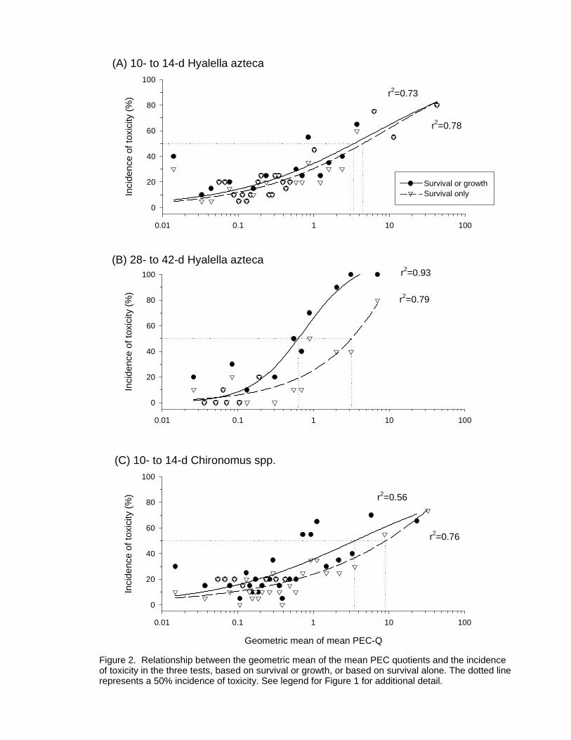
27

0.01 0.1 1 10 100

Inci

denc

eof

toxi

city

(%)

0

20

40

60

80

100

Survival or growthSurvival only

(A) 10- to 14-d Hyalella azteca

0.01 0.1 1 10 100

Inci

denc

eof

toxi

city

(%)

0

20

40

60

80

100

(B) 28- to 42-d Hyalella azteca

Geometric mean of mean PEC-Q

0.01 0.1 1 10 100

Inci

denc

eof

toxi

city

(%)

0

20

40

60

80

100

(C) 10- to 14-d Chironomus spp.

r2=0.73

r2=0.78

r2=0.93

r2=0.79

r2=0.76

r2=0.56

Figure 2. Relationship between the geometric mean of the mean PEC quotients and the incidenceof toxicity in the three tests, based on survival or growth, or based on survival alone. The dotted linerepresents a 50% incidence of toxicity. See legend for Figure 1 for additional detail.

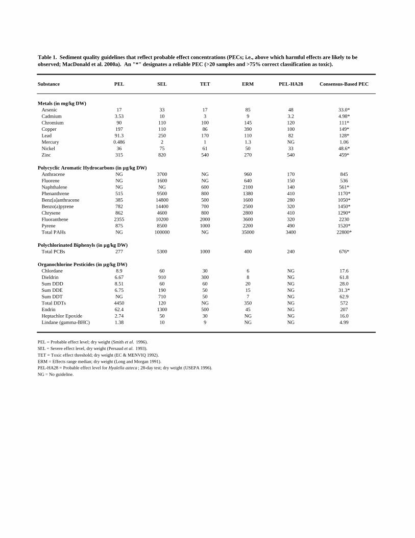
Table 1. Sediment quality guidelines that reflect probable effect concentrations (PECs; i.e., above which harmful effects are likely to be observed; MacDonald et al. 2000a). An "*" designates a reliable PEC (>20 samples and >75% correct classification as toxic).

Substance PEL SEL TET ERM PEL-HA28 Consensus-Based PEC

Metals (in mg/kg DW) Arsenic 17 33 17 85 48 33.0* Cadmium 3.53 10 3 9 3.2 4.98* Chromium 90 110 100 145 120 111* Copper 197 110 86 390 100 149* Lead 91.3 250 170 110 82 128* Mercury 0.486 2 1 1.3 NG 1.06 Nickel 36 75 61 50 33 48.6* Zinc 315 820 540 270 540 459*

Polycyclic Aromatic Hydrocarbons (in µg/kg DW) Anthracene NG 3700 NG 960 170 845 Fluorene NG 1600 NG 640 150 536 Naphthalene NG NG 600 2100 140 561* Phenanthrene 515 9500 800 1380 410 1170* Benz[a]anthracene 385 14800 500 1600 280 1050* Benzo(a)pyrene 782 14400 700 2500 320 1450* Chrysene 862 4600 800 2800 410 1290* Fluoranthene 2355 10200 2000 3600 320 2230 Pyrene 875 8500 1000 2200 490 1520* Total PAHs NG 100000 NG 35000 3400 22800*

Polychlorinated Biphenyls (in µg/kg DW) Total PCBs 277 5300 1000 400 240 676*

Organochlorine Pesticides (in µg/kg DW) Chlordane 8.9 60 30 6 NG 17.6 Dieldrin 6.67 910 300 8 NG 61.8 Sum DDD 8.51 60 60 20 NG 28.0 Sum DDE 6.75 190 50 15 NG 31.3* Sum DDT NG 710 50 7 NG 62.9 Total DDTs 4450 120 NG 350 NG 572 Endrin 62.4 1300 500 45 NG 207 Heptachlor Epoxide 2.74 50 30 NG NG 16.0 Lindane (gamma-BHC) 1.38 10 9 NG NG 4.99

PEL = Probable effect level; dry weight (Smith et al. 1996).

SEL = Severe effect level, dry weight (Persaud et al. 1993).

TET = Toxic effect threshold; dry weight (EC & MENVIQ 1992).

ERM = Effects range median; dry weight (Long and Morgan 1991).PEL-HA28 = Probable effect level for Hyalella azteca ; 28-day test; dry weight (USEPA 1996).

NG = No guideline.

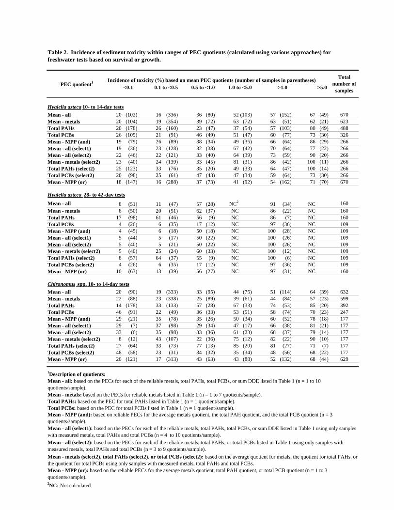
Table 2. Incidence of sediment toxicity within ranges of PEC quotients (calculated using various approaches) for freshwater tests based on survival or growth.

Total PEC quotient1 Incidence of toxicity (%) based on mean PEC quotients (number of samples in parentheses)

number of <0.1 0.1 to <0.5 0.5 to <1.0 1.0 to <5.0 >1.0 >5.0

samples

Hyalella azteca 10- to 14-day tests

Mean - all 20 (102) 16 (336) 36 (80) 52 (103) 57 (152) 67 (49) 670 Mean - metals 20 (104) 19 (354) 39 (72) 63 (72) 63 (51) 62 (21) 623 Total PAHs 20 (178) 26 (160) 23 (47) 37 (54) 57 (103) 80 (49) 488 Total PCBs 26 (109) 21 (91) 46 (49) 51 (47) 60 (77) 73 (30) 326 Mean - MPP (and) 19 (79) 26 (89) 38 (34) 49 (35) 66 (64) 86 (29) 266 Mean - all (select1) 19 (36) 23 (128) 32 (38) 67 (42) 70 (64) 77 (22) 266 Mean - all (select2) 22 (46) 22 (121) 33 (40) 64 (39) 73 (59) 90 (20) 266 Mean - metals (select2) 23 (40) 24 (139) 33 (45) 81 (31) 86 (42) 100 (11) 266 Total PAHs (select2) 25 (123) 33 (76) 35 (20) 49 (33) 64 (47) 100 (14) 266 Total PCBs (select2) 20 (98) 25 (61) 47 (43) 47 (34) 59 (64) 73 (30) 266 Mean - MPP (or) 18 (147) 16 (288) 37 (73) 41 (92) 54 (162) 71 (70) 670

Hyalella azteca 28- to 42-day tests

Mean - all 8 (51) 11 (47) 57 (28) NC2 91 (34) NC 160

Mean - metals 8 (50) 20 (51) 62 (37) NC 86 (22) NC 160 Total PAHs 17 (98) 61 (46) 56 (9) NC 86 (7) NC 160 Total PCBs 4 (26) 6 (35) 17 (12) NC 97 (36) NC 109 Mean - MPP (and) 4 (45) 6 (18) 50 (18) NC 100 (28) NC 109 Mean - all (select1) 5 (44) 5 (17) 50 (22) NC 100 (26) NC 109 Mean - all (select2) 5 (40) 5 (21) 50 (22) NC 100 (26) NC 109 Mean - metals (select2) 5 (40) 25 (24) 60 (33) NC 100 (12) NC 109 Total PAHs (select2) 8 (57) 64 (37) 55 (9) NC 100 (6) NC 109 Total PCBs (select2) 4 (26) 6 (35) 17 (12) NC 97 (36) NC 109 Mean - MPP (or) 10 (63) 13 (39) 56 (27) NC 97 (31) NC 160

Chironomus spp. 10- to 14-day tests

Mean - all 20 (90) 19 (333) 33 (95) 44 (75) 51 (114) 64 (39) 632 Mean - metals 22 (88) 23 (338) 25 (89) 39 (61) 44 (84) 57 (23) 599 Total PAHs 14 (178) 33 (133) 57 (28) 67 (33) 74 (53) 85 (20) 392 Total PCBs 46 (91) 22 (49) 36 (33) 53 (51) 58 (74) 70 (23) 247 Mean - MPP (and) 29 (21) 35 (78) 35 (26) 50 (34) 60 (52) 78 (18) 177 Mean - all (select1) 29 (7) 37 (98) 29 (34) 47 (17) 66 (38) 81 (21) 177 Mean - all (select2) 33 (6) 35 (98) 33 (36) 61 (23) 68 (37) 79 (14) 177 Mean - metals (select2) 8 (12) 43 (107) 22 (36) 75 (12) 82 (22) 90 (10) 177 Total PAHs (select2) 27 (64) 33 (73) 77 (13) 85 (20) 81 (27) 71 (7) 177 Total PCBs (select2) 48 (58) 23 (31) 34 (32) 35 (34) 48 (56) 68 (22) 177 Mean - MPP (or) 20 (121) 17 (313) 43 (63) 43 (88) 52 (132) 68 (44) 629

1Description of quotients:Mean - all: based on the PECs for each of the reliable metals, total PAHs, total PCBs, or sum DDE listed in Table 1 (n = 1 to 10quotients/sample).Mean - metals: based on the PECs for reliable metals listed in Table 1 (n = 1 to 7 quotients/sample).Total PAHs: based on the PEC for total PAHs listed in Table 1 (n = 1 quotient/sample).Total PCBs: based on the PEC for total PCBs listed in Table 1 (n = 1 quotient/sample).Mean - MPP (and): based on reliable PECs for the average metals quotient, the total PAH quotient, and the total PCB quotient (n = 3quotients/sample).Mean - all (select1): based on the PECs for each of the reliable metals, total PAHs, total PCBs, or sum DDE listed in Table 1 using only sampleswith measured metals, total PAHs and total PCBs (n = 4 to 10 quotients/sample).Mean - all (select2): based on the PECs for each of the reliable metals, total PAHs, or total PCBs listed in Table 1 using only samples withmeasured metals, total PAHs and total PCBs (n = 3 to 9 quotients/sample).

Mean - metals (select2), total PAHs (select2), or total PCBs (select2): based on the average quotient for metals, the quotient for total PAHs, orthe quotient for total PCBs using only samples with measured metals, total PAHs and total PCBs.Mean - MPP (or): based on the reliable PECs for the average metals quotient, total PAH quotient, or total PCB quotient (n = 1 to 3 quotients/sample). 2NC: Not calculated.

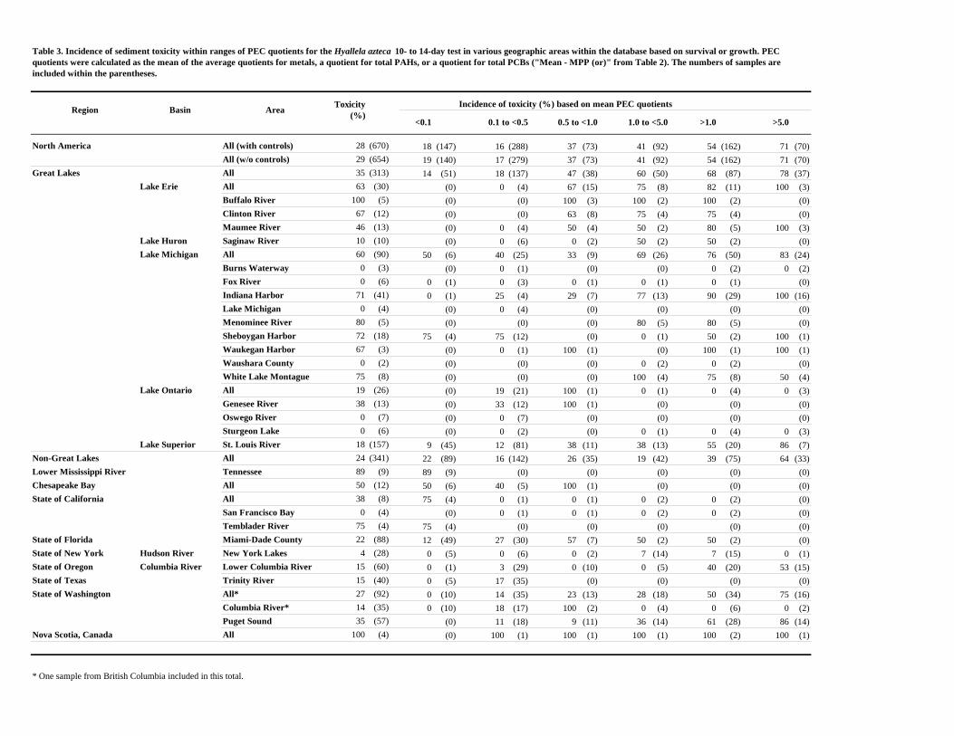
Table 3. Incidence of sediment toxicity within ranges of PEC quotients for the Hyallela azteca 10- to 14-day test in various geographic areas within the database based on survival or growth. PEC quotients were calculated as the mean of the average quotients for metals, a quotient for total PAHs, or a quotient for total PCBs ("Mean - MPP (or)" from Table 2). The numbers of samples are included within the parentheses.

Region Basin Area Toxicity

(%) Incidence of toxicity (%) based on mean PEC quotients

<0.1 0.1 to <0.5 0.5 to <1.0 1.0 to <5.0 >1.0 >5.0

North America All (with controls) 28 (670) 18 (147) 16 (288) 37 (73) 41 (92) 54 (162) 71 (70)

All (w/o controls) 29 (654) 19 (140) 17 (279) 37 (73) 41 (92) 54 (162) 71 (70)

Great Lakes All 35 (313) 14 (51) 18 (137) 47 (38) 60 (50) 68 (87) 78 (37)

Lake Erie All 63 (30) (0) 0 (4) 67 (15) 75 (8) 82 (11) 100 (3)

Buffalo River 100 (5) (0) (0) 100 (3) 100 (2) 100 (2) (0)

Clinton River 67 (12) (0) (0) 63 (8) 75 (4) 75 (4) (0)

Maumee River 46 (13) (0) 0 (4) 50 (4) 50 (2) 80 (5) 100 (3)

Lake Huron Saginaw River 10 (10) (0) 0 (6) 0 (2) 50 (2) 50 (2) (0)

Lake Michigan All 60 (90) 50 (6) 40 (25) 33 (9) 69 (26) 76 (50) 83 (24)

Burns Waterway 0 (3) (0) 0 (1) (0) (0) 0 (2) 0 (2)

Fox River 0 (6) 0 (1) 0 (3) 0 (1) 0 (1) 0 (1) (0)

Indiana Harbor 71 (41) 0 (1) 25 (4) 29 (7) 77 (13) 90 (29) 100 (16)

Lake Michigan 0 (4) (0) 0 (4) (0) (0) (0) (0)

Menominee River 80 (5) (0) (0) (0) 80 (5) 80 (5) (0)

Sheboygan Harbor 72 (18) 75 (4) 75 (12) (0) 0 (1) 50 (2) 100 (1)

Waukegan Harbor 67 (3) (0) 0 (1) 100 (1) (0) 100 (1) 100 (1)

Waushara County 0 (2) (0) (0) (0) 0 (2) 0 (2) (0)

White Lake Montague 75 (8) (0) (0) (0) 100 (4) 75 (8) 50 (4)

Lake Ontario All 19 (26) (0) 19 (21) 100 (1) 0 (1) 0 (4) 0 (3)

Genesee River 38 (13) (0) 33 (12) 100 (1) (0) (0) (0)

Oswego River 0 (7) (0) 0 (7) (0) (0) (0) (0)

Sturgeon Lake 0 (6) (0) 0 (2) (0) 0 (1) 0 (4) 0 (3)

Lake Superior St. Louis River 18 (157) 9 (45) 12 (81) 38 (11) 38 (13) 55 (20) 86 (7)

Non-Great Lakes All 24 (341) 22 (89) 16 (142) 26 (35) 19 (42) 39 (75) 64 (33)

Lower Mississippi River Tennessee 89 (9) 89 (9) (0) (0) (0) (0) (0)

Chesapeake Bay All 50 (12) 50 (6) 40 (5) 100 (1) (0) (0) (0)

State of California All 38 (8) 75 (4) 0 (1) 0 (1) 0 (2) 0 (2) (0)

San Francisco Bay 0 (4) (0) 0 (1) 0 (1) 0 (2) 0 (2) (0)

Temblader River 75 (4) 75 (4) (0) (0) (0) (0) (0)

State of Florida Miami-Dade County 22 (88) 12 (49) 27 (30) 57 (7) 50 (2) 50 (2) (0)

State of New York Hudson River New York Lakes 4 (28) 0 (5) 0 (6) 0 (2) 7 (14) 7 (15) 0 (1)

State of Oregon Columbia River Lower Columbia River 15 (60) 0 (1) 3 (29) 0 (10) 0 (5) 40 (20) 53 (15)

State of Texas Trinity River 15 (40) 0 (5) 17 (35) (0) (0) (0) (0)

State of Washington All* 27 (92) 0 (10) 14 (35) 23 (13) 28 (18) 50 (34) 75 (16)

Columbia River* 14 (35) 0 (10) 18 (17) 100 (2) 0 (4) 0 (6) 0 (2)

Puget Sound 35 (57) (0) 11 (18) 9 (11) 36 (14) 61 (28) 86 (14)

Nova Scotia, Canada All 100 (4) (0) 100 (1) 100 (1) 100 (1) 100 (2) 100 (1)

* One sample from British Columbia included in this total.

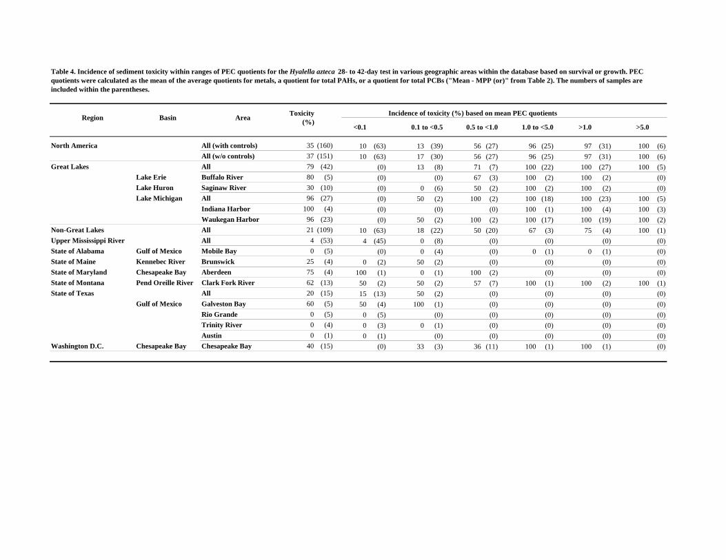
Table 4. Incidence of sediment toxicity within ranges of PEC quotients for the Hyalella azteca 28- to 42-day test in various geographic areas within the database based on survival or growth. PEC quotients were calculated as the mean of the average quotients for metals, a quotient for total PAHs, or a quotient for total PCBs ("Mean - MPP (or)" from Table 2). The numbers of samples are included within the parentheses.

Region Basin Area Toxicity

(%) <0.1

Incidence of toxicity (%) based on mean PEC quotients

0.1 to <0.5 0.5 to <1.0 1.0 to <5.0 >1.0 >5.0

North America All (with controls) 35 (160) 10 (63) 13 (39) 56 (27) 96 (25) 97 (31) 100 (6)

All (w/o controls) 37 (151) 10 (63) 17 (30) 56 (27) 96 (25) 97 (31) 100 (6)

Great Lakes All 79 (42) (0) 13 (8) 71 (7) 100 (22) 100 (27) 100 (5)

Lake Erie Buffalo River 80 (5) (0) (0) 67 (3) 100 (2) 100 (2) (0)

Lake Huron Saginaw River 30 (10) (0) 0 (6) 50 (2) 100 (2) 100 (2) (0)

Lake Michigan All 96 (27) (0) 50 (2) 100 (2) 100 (18) 100 (23) 100 (5)

Indiana Harbor 100 (4) (0) (0) (0) 100 (1) 100 (4) 100 (3)

Waukegan Harbor 96 (23) (0) 50 (2) 100 (2) 100 (17) 100 (19) 100 (2)

Non-Great Lakes All 21 (109) 10 (63) 18 (22) 50 (20) 67 (3) 75 (4) 100 (1)

Upper Mississippi River All 4 (53) 4 (45) 0 (8) (0) (0) (0) (0)

State of Alabama Gulf of Mexico Mobile Bay 0 (5) (0) 0 (4) (0) 0 (1) 0 (1) (0)

State of Maine Kennebec River Brunswick 25 (4) 0 (2) 50 (2) (0) (0) (0) (0)

State of Maryland Chesapeake Bay Aberdeen 75 (4) 100 (1) 0 (1) 100 (2) (0) (0) (0)

State of Montana Pend Oreille River Clark Fork River 62 (13) 50 (2) 50 (2) 57 (7) 100 (1) 100 (2) 100 (1)

State of Texas All 20 (15) 15 (13) 50 (2) (0) (0) (0) (0)

Gulf of Mexico Galveston Bay 60 (5) 50 (4) 100 (1) (0) (0) (0) (0)

Rio Grande 0 (5) 0 (5) (0) (0) (0) (0) (0)

Trinity River 0 (4) 0 (3) 0 (1) (0) (0) (0) (0)

Austin 0 (1) 0 (1) (0) (0) (0) (0) (0)

Washington D.C. Chesapeake Bay Chesapeake Bay 40 (15) (0) 33 (3) 36 (11) 100 (1) 100 (1) (0)

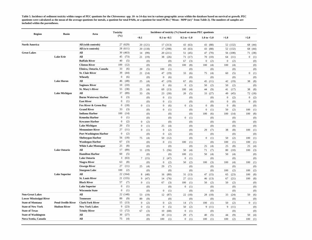
Table 5. Incidence of sediment toxicity within ranges of PEC quotients for the Chironomus spp. 10- to 14-day test in various geographic areas within the database based on survival or growth. PEC quotients were calculated as the mean of the average quotients for metals, a quotient for total PAHs, or a quotient for total PCBs ("Mean - MPP (or)" from Table 2). The numbers of samples are included within the parentheses.

Region Basin Area Toxicity

(%) Incidence of toxicity (%) based on mean PEC quotients

<0.1 0.1 to <0.5 0.5 to <1.0 1.0 to <5.0 >1.0 >5.0

North America All (with controls) 27 (629) 20 (121) 17 (313) 43 (63) 43 (88) 52 (132) 68 (44)

All (w/o controls) 28 (611) 20 (118) 17 (298) 43 (63) 43 (88) 52 (132) 68 (44)

Great Lakes All 30 (463) 14 (99) 20 (211) 51 (45) 47 (70) 56 (108) 71 (38)

Lake Erie All 45 (73) 21 (19) 38 (26) 71 (17) 70 (10) 64 (11) 0 (1)

Buffalo River 40 (5) (0) (0) 67 (3) 0 (2) 0 (2) (0)

Clinton River 100 (12) (0) (0) 100 (8) 100 (4) 100 (4) (0)

Elmira, Ontario, Canada 33 (6) 20 (5) 100 (1) (0) (0) (0) (0)

St. Clair River 39 (44) 21 (14) 47 (19) 33 (6) 75 (4) 60 (5) 0 (1)

Wheatly 0 (6) (0) 0 (6) (0) (0) (0) (0)

Lake Huron All 46 (48) 25 (4) 47 (19) 67 (6) 45 (11) 42 (19) 38 (8)

Saginaw River 10 (10) (0) 0 (6) 0 (2) 50 (2) 50 (2) (0)

St. Mary's River 55 (38) 25 (4) 69 (13) 100 (4) 44 (9) 41 (17) 38 (8)

Lake Michigan All 37 (89) 33 (9) 23 (30) 20 (5) 33 (27) 49 (45) 72 (18)

Burns Waterway Harbor 0 (3) (0) 0 (1) (0) (0) 0 (2) 0 (2)

East River 0 (1) (0) 0 (1) (0) (0) 0 (0) 0 (0)

Fox River & Green Bay 0 (18) 0 (1) 0 (6) 0 (3) 0 (8) 0 (8) (0)

Grand River 33 (3) (0) 0 (1) (0) 0 (1) 50 (2) 100 (1)

Indiana Harbor 100 (14) (0) (0) (0) 100 (6) 100 (14) 100 (8)

Kenosha Harbor 0 (1) (0) (0) 0 (1) (0) (0) (0)

Kewanee Harbor 0 (2) 0 (2) (0) (0) (0) (0) (0)

Lake Michigan 20 (5) 0 (1) 25 (4) (0) (0) (0) (0)

Menominee River 27 (11) 0 (1) 0 (2) (0) 29 (7) 38 (8) 100 (1)

Port Washington Harbor 0 (2) (0) 0 (2) (0) (0) (0) (0)

Sheboygan Harbor 56 (18) 75 (4) 50 (12) (0) 0 (1) 50 (2) 100 (1)

Waukegan Harbor 67 (3) (0) 0 (1) 100 (1) (0) 100 (1) 100 (1)

White Lake Montague 25 (8) (0) (0) (0) 25 (4) 25 (8) 25 (4)

Lake Ontario All 17 (89) 11 (19) 5 (56) 50 (4) 71 (7) 80 (10) 100 (3)

Hamilton Harbor 60 (5) (0) (0) 100 (1) 50 (4) 50 (4) (0)

Lake Ontario 3 (63) 7 (15) 2 (47) 0 (1) (0) (0) (0)

Niagra River 63 (8) (0) 0 (2) 50 (2) 100 (3) 100 (4) 100 (1)

Oswego River 27 (11) 25 (4) 29 (7) (0) (0) (0) (0)

Sturgeon Lake 100 (2) (0) (0) (0) (0) 100 (2) 100 (2)

Lake Superior All 22 (164) 8 (48) 16 (80) 31 (13) 47 (15) 65 (23) 100 (8)

St. Louis River 21 (155) 9 (47) 14 (76) 27 (11) 46 (13) 67 (21) 100 (8)

Black River 57 (7) 0 (1) 67 (3) 100 (1) 50 (2) 50 (2) (0)

Lake Superior 0 (1) (0) (0) 0 (1) (0) (0) (0)

Wisconsin State 0 (1) (0) 0 (1) (0) (0) (0) (0)

Non-Great Lakes All 22 (148) 53 (19) 12 (87) 22 (18) 28 (18) 33 (24) 50 (6)

Lower Mississippi River Tennessee 89 (9) 89 (9) (0) (0) (0) (0) (0)

State of Montana Pend Oreille River Clark Fork River 15 (13) 0 (2) 0 (2) 14 (7) 100 (1) 50 (2) 0 (1)

State of New York Hudson River New York Lakes 9 (23) 0 (5) 0 (5) 50 (2) 9 (11) 9 (11) (0)

State of Texas Trinity River 13 (72) 67 (3) 10 (68) 0 (1) (0) (0) (0)

State of Washington All 30 (27) (0) 18 (11) 29 (7) 40 (5) 44 (9) 50 (4)

Nova Scotia, Canada All 75 (4) (0) 100 (1) 0 (1) 100 (1) 100 (2) 100 (1)

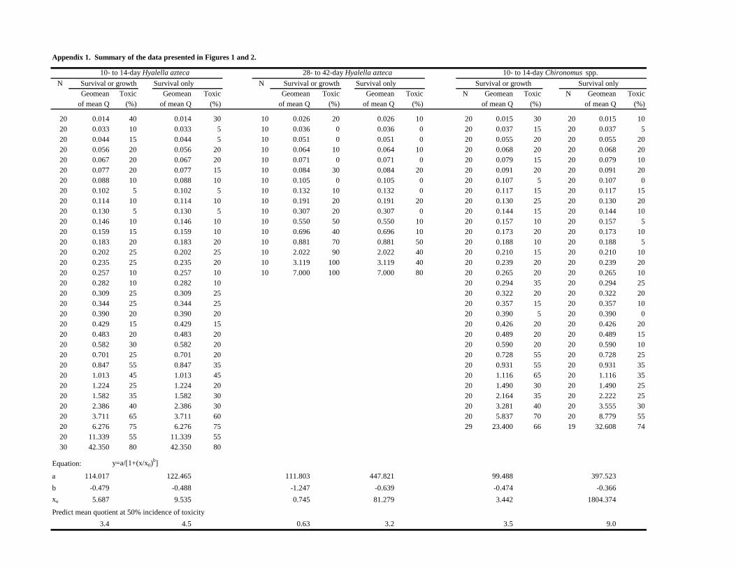
Appendix 1. Summary of the data presented in Figures 1 and 2.

10- to 14-day Hyalella azteca 28- to 42-day Hyalella azteca 10- to 14-day Chironomus spp.

N Survival or growth Survival only N Survival or growth Survival only Survival or growth Survival only Geomean Toxic Geomean Toxic Geomean Toxic Geomean Toxic N Geomean Toxic N Geomean Toxic

of mean Q (%) of mean Q (%) of mean Q (%) of mean Q (%) of mean Q (%) of mean Q (%)

20 0.014 40 0.014 30 10 0.026 20 0.026 10 20 0.015 30 20 0.015 10 20 0.033 10 0.033 5 10 0.036 0 0.036 0 20 0.037 15 20 0.037 5 20 0.044 15 0.044 5 10 0.051 0 0.051 0 20 0.055 20 20 0.055 20 20 0.056 20 0.056 20 10 0.064 10 0.064 10 20 0.068 20 20 0.068 20 20 0.067 20 0.067 20 10 0.071 0 0.071 0 20 0.079 15 20 0.079 10 20 0.077 20 0.077 15 10 0.084 30 0.084 20 20 0.091 20 20 0.091 20 20 0.088 10 0.088 10 10 0.105 0 0.105 0 20 0.107 5 20 0.107 0 20 0.102 5 0.102 5 10 0.132 10 0.132 0 20 0.117 15 20 0.117 15 20 0.114 10 0.114 10 10 0.191 20 0.191 20 20 0.130 25 20 0.130 20 20 0.130 5 0.130 5 10 0.307 20 0.307 0 20 0.144 15 20 0.144 10 20 0.146 10 0.146 10 10 0.550 50 0.550 10 20 0.157 10 20 0.157 5 20 0.159 15 0.159 10 10 0.696 40 0.696 10 20 0.173 20 20 0.173 10 20 0.183 20 0.183 20 10 0.881 70 0.881 50 20 0.188 10 20 0.188 5 20 0.202 25 0.202 25 10 2.022 90 2.022 40 20 0.210 15 20 0.210 10 20 0.235 25 0.235 20 10 3.119 100 3.119 40 20 0.239 20 20 0.239 20 20 0.257 10 0.257 10 10 7.000 100 7.000 80 20 0.265 20 20 0.265 10 20 0.282 10 0.282 10 20 0.294 35 20 0.294 25 20 0.309 25 0.309 25 20 0.322 20 20 0.322 20 20 0.344 25 0.344 25 20 0.357 15 20 0.357 10 20 0.390 20 0.390 20 20 0.390 5 20 0.390 0 20 0.429 15 0.429 15 20 0.426 20 20 0.426 20 20 0.483 20 0.483 20 20 0.489 20 20 0.489 15 20 0.582 30 0.582 20 20 0.590 20 20 0.590 10 20 0.701 25 0.701 20 20 0.728 55 20 0.728 25 20 0.847 55 0.847 35 20 0.931 55 20 0.931 35 20 1.013 45 1.013 45 20 1.116 65 20 1.116 35 20 1.224 25 1.224 20 20 1.490 30 20 1.490 25 20 1.582 35 1.582 30 20 2.164 35 20 2.222 25 20 2.386 40 2.386 30 20 3.281 40 20 3.555 30 20 3.711 65 3.711 60 20 5.837 70 20 8.779 55 20 6.276 75 6.276 75 29 23.400 66 19 32.608 74 20 11.339 55 11.339 55 30 42.350 80 42.350 80

Equation: y=a/[1+(x/x0)b]

a 114.017 122.465 111.803 447.821 99.488 397.523

b -0.479 -0.488 -1.247 -0.639 -0.474 -0.366

xo 5.687 9.535 0.745 81.279 3.442 1804.374

Predict mean quotient at 50% incidence of toxicity

3.4 4.5 0.63 3.2 3.5 9.0