Prediction of post overload fatigue crack growth life of …ijecs.in/issue/v5-i11/25 ijecs.pdfvariable amplitude loads, block loads etc. In real situations, ... different angles of

www.ijecs.in

International Journal Of Engineering And Computer Science ISSN: 2319-7242

Volume 5 Issue 11 Nov. 2016, Page No. 18856-18870

J. R. Mohanty, IJECS Volume 05 Issue 11 Nov., 2016 Page No.18856-18870 Page 18856

Prediction of post overload fatigue crack growth life of HSLA steel under mixed-mode (I

and II) spike overload by using genetic programming

J. R. Mohanty

Department of Mechanical Engineering

Veer Surendra Sai University, Burla, Sambalpur (Odisha) 768018, India

Email address: [email protected]

Abstract

In the present investigation, fatigue crack growth tests under mixed-mode (I and II) overload have been

conducted on HSLA steel and subsequently genetic programming has been applied to predict post overload

fatigue life. It is observed that the proposed model predicts fatigue life of HSLA steel with reasonable accuracy.

Keywords: Genetic programming; Delay cycle; Mixed-mode; HSLA steel; Fatigue life;

1. INTRODUCTION

High strength low alloy (HSLA) steels are designed and developed to provide better mechanical

properties and greater resistance to atmospheric corrosion than conventional carbon steels. They have high

strength, toughness, weldability, formability and corrosion resistance which render them suitable for use in a

wide variety of structural applications. These structural components are frequently subjected to cyclic loading

during their service lives which causes fatigue failure. As the failure due to fatigue is one of the prime concerns

in structural design, its evaluation and prediction of fatigue life is thus very important to avoid catastrophic

failure. For this purpose, the principles of fracture mechanics are used to determine whether the cracks will

grow large enough to cause catastrophic failure before they can be detected during a periodic inspection. To

predict fatigue crack growth life a large data base has to be created which requires large number of fatigue tests

on varieties of materials. However, these tests are costly and also time consuming. With the advent of

sophisticated computational facilities, now a day, alternative methods have been designed and developed to

predict fatigue life based on experimental base line data in order to avoid costly fatigue tests.

Fatigue crack propagation is a path dependent process and is strongly affected by the load sequence [1].

The load sequence may consist of simple constant amplitude load, superimposed overloads and under loads,

variable amplitude loads, block loads etc. In real situations, components and structures are frequently exposed

DOI: 10.18535/ijecs/v5i11.25


to complex stress field because of the inconsistent variation of applied fatigue loads and the mode-mixity. Over

many years, there have been many studies on crack behavior under complex stress fields [2–5]. However,

studies on load interactions (particularly superimposed overloads) under mixed-mode (I and II) loading

conditions [6–9] on fatigue behavior are still limited. As far as prediction of fatigue life under interspersed

mixed-mode (I and II) overload is concerned, it is a complex phenomena due to the interaction effects that exist

during fatigue crack growth under this loading situation. Therefore, evolutionary computational methods such

as artificial neural network (ANN), genetic algorithm (GA), fuzzy-logic, adaptive neuo-fuzzy inference system

(ANFIS) etc. have emerged as alternative modeling tools in the field of fatigue. Genel [10] has applied ANN for

predicting the strain-life fatigue properties using tensile material data of steels. Fotovati and Goswami [11] have

used ANN approach to predict fatigue crack growth rate in Ti-6Al-4V alloy at elevated temperature. Jarrah et

al. [12] has applied ANFIS to model the fatigue behavior of unidirectional glass fiber / epoxy composites under

tension-tension and tension-compression loading. Genetic programming (GP) has been applied by

Vassilopoulos and Georgopoulos [13] in modeling fatigue life of FRP composite materials. As far as prediction

of fatigue crack growth life under mixed-mode (I and II) by GP is concerned, almost no work has been reported

till date. Thus, the present investigation aims at developing GP model to predict post overload fatigue crack

growth life of HSLA (ASTM A633 Gr. A) steel under the above loading condition.

2. EXPERIMENTATION

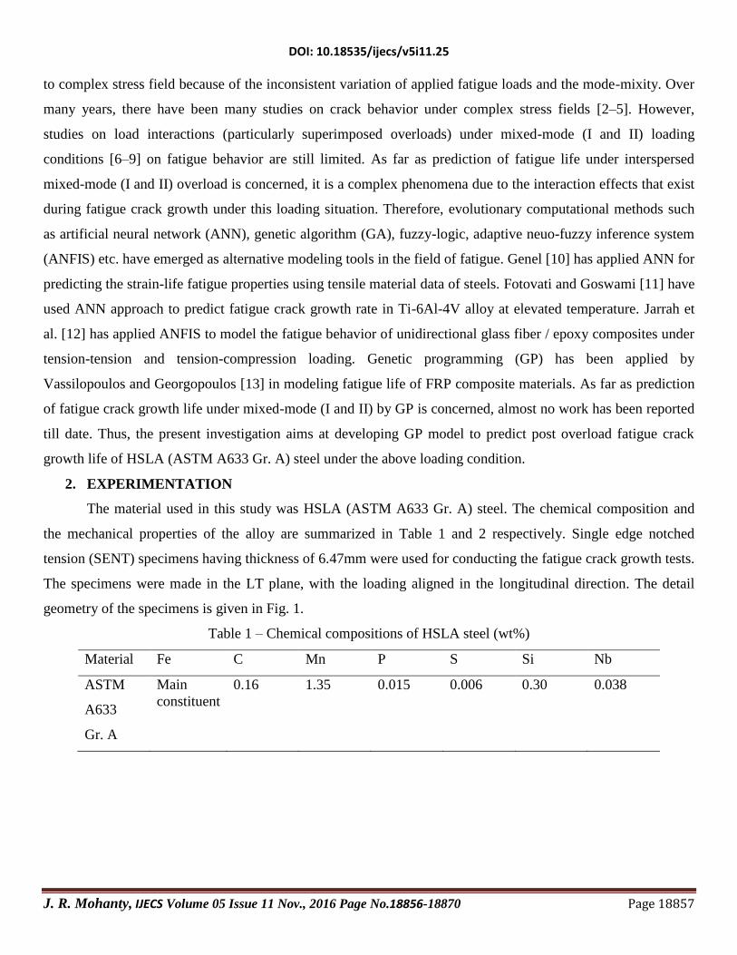
The material used in this study was HSLA (ASTM A633 Gr. A) steel. The chemical composition and

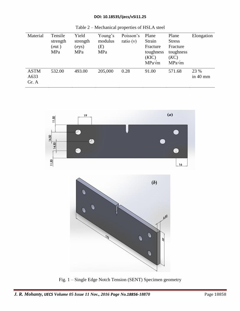
the mechanical properties of the alloy are summarized in Table 1 and 2 respectively. Single edge notched

tension (SENT) specimens having thickness of 6.47mm were used for conducting the fatigue crack growth tests.

The specimens were made in the LT plane, with the loading aligned in the longitudinal direction. The detail

geometry of the specimens is given in Fig. 1.

Table 1 – Chemical compositions of HSLA steel (wt%)

Material Fe C Mn P S Si Nb

ASTM

A633

Gr. A

Main

constituent

0.16 1.35 0.015 0.006 0.30 0.038

DOI: 10.18535/ijecs/v5i11.25


Table 2 – Mechanical properties of HSLA steel

Material Tensile

strength

(σut )

MPa

Yield

strength

(σys)

MPa

Young‟s

modulus

(E)

MPa

Poisson‟s

ratio (ν)

Plane

Strain

Fracture

toughness

(KIC)

MPa√m

Plane

Stress

Fracture

toughness

(KC)

MPa√m

Elongation

ASTM

A633

Gr. A

532.00 493.00 205,000 0.28 91.00 571.68 23 %

in 40 mm

Fig. 1 – Single Edge Notch Tension (SENT) Specimen geometry

DOI: 10.18535/ijecs/v5i11.25


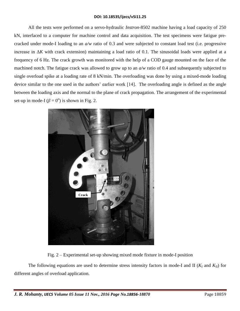
All the tests were performed on a servo-hydraulic Instron-8502 machine having a load capacity of 250

kN, interfaced to a computer for machine control and data acquisition. The test specimens were fatigue pre-

cracked under mode-I loading to an a/w ratio of 0.3 and were subjected to constant load test (i.e. progressive

increase in ΔK with crack extension) maintaining a load ratio of 0.1. The sinusoidal loads were applied at a

frequency of 6 Hz. The crack growth was monitored with the help of a COD gauge mounted on the face of the

machined notch. The fatigue crack was allowed to grow up to an a/w ratio of 0.4 and subsequently subjected to

single overload spike at a loading rate of 8 kN/min. The overloading was done by using a mixed-mode loading

device similar to the one used in the authors‟ earlier work [14]. The overloading angle is defined as the angle

between the loading axis and the normal to the plane of crack propagation. The arrangement of the experimental

set-up in mode-I (β = 0o) is shown in Fig. 2.

Fig. 2 – Experimental set-up showing mixed mode fixture in mode-I position

The following equations are used to determine stress intensity factors in mode-I and II (KI and KII) for

different angles of overload application.

Crack

DOI: 10.18535/ijecs/v5i11.25


wB

aFgfK

.cos).(I (1)

wB

aFgfK

.sin).(II (2) where,

432 )/(39.30)/(72.21)/(55.10)/(231.012.1)( wawawawagf

The specimens were subjected to mode I, mode II, and mixed-mode overloads at different loading angles, β (=

18o, 36

o, 54

o and 72

o) at an overloading ratio of 2.5. Overloading ratio is defined as

BK

KR

max

ol

eqol (3)

where BKmax is the maximum stress intensity factor for base line test. The equivalent stress intensity factors ol

eqK

are calculated according to the following equation:

2ol

II1

2ol

I

ol

I

ol

eq 45.05.0 KKKK (4)

where α1 = (KIC/KIIC) = 0.95 according to strain energy density theory and KIol

and ol

IIK are the of stress intensity

factors of modes I and II during the overload respectively. Then the fatigue test was continued in mode I. Since,

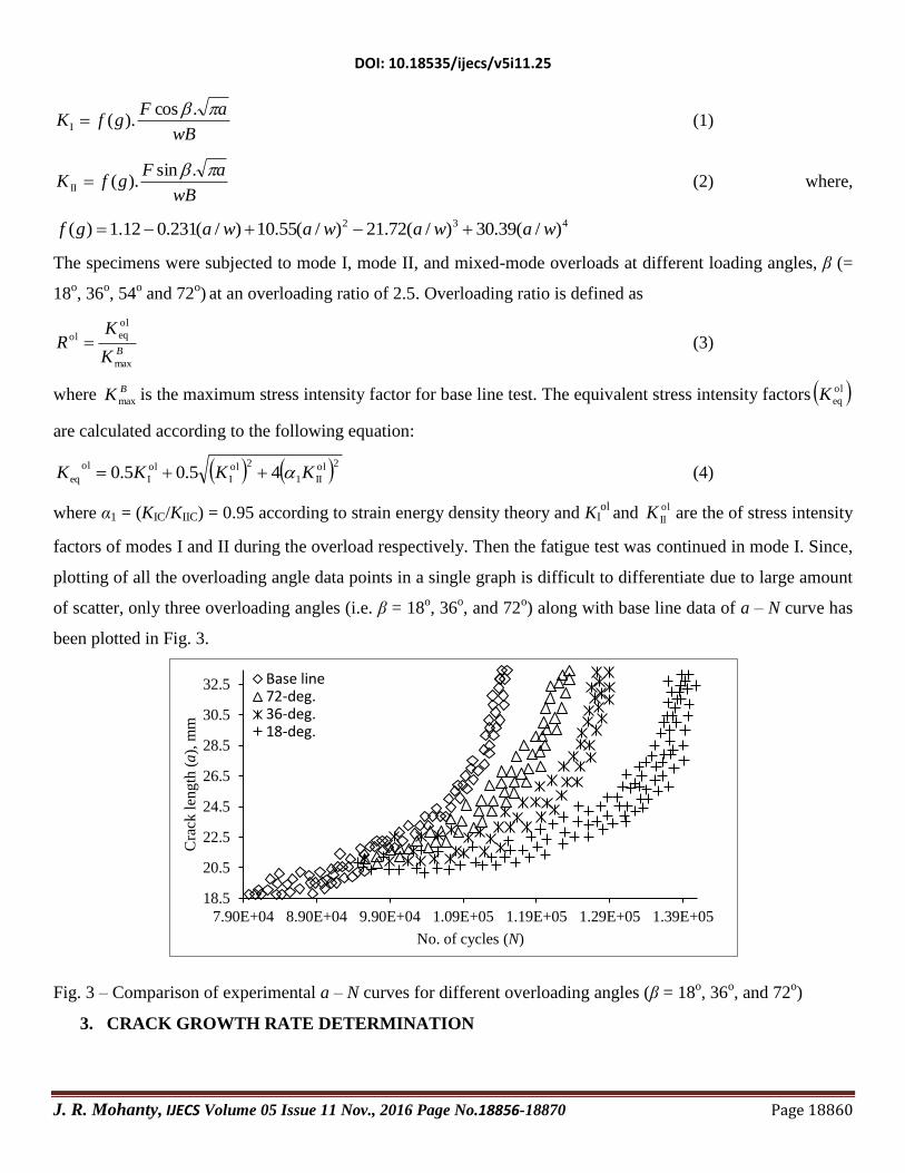
plotting of all the overloading angle data points in a single graph is difficult to differentiate due to large amount

of scatter, only three overloading angles (i.e. β = 18o, 36

o, and 72

o) along with base line data of a – N curve has

been plotted in Fig. 3.

Fig. 3 – Comparison of experimental a – N curves for different overloading angles (β = 18o, 36

o, and 72

o)

3. CRACK GROWTH RATE DETERMINATION

18.5

20.5

22.5

24.5

26.5

28.5

30.5

32.5

7.90E+04 8.90E+04 9.90E+04 1.09E+05 1.19E+05 1.29E+05 1.39E+05

Cra

ck l

ength

(a),

mm

No. of cycles (N)

Base line72-deg.36-deg.18-deg.

DOI: 10.18535/ijecs/v5i11.25


The determination of fatigue crack growth rate (da/dN) from raw laboratory data (shown in Fig. 3 as a

sample copy) is of course a tedious task because of large amount of scatter. Out of various techniques proposed

till date, the exponential equation method [15] has been proved to be better as it is possible to fit the entire a - N

data in a single equation. The same method has been adopted in this work to determine the crack growth rate

which is described below.

It has been already established [15] that the experimental a - N data can be well fitted by an exponential

equation of the form:

)(

ijijij NNm

eaa

(5)

where, ai and aj = crack length in ith

step and jth

step in „mm‟ respectively,

Ni and Nj = No. of cycles in ith

step and jth

step respectively,

mij= specific growth rate in the interval i-j,

i = No. of experimental steps,

and j = i+1

In the above equation the exponent „mij‟(i.e. specific growth rate) is an important parameter which can be

obtained by taking logarithm of equation (5) as follows:

ij

i

j

ij

ln

NN

a

a

m

(6)

The raw values of specific growth rate (mij) from experimental a–N data are calculated using the above

equation. These are then fitted with corresponding crack lengths by a polynomial curve-fit which gives a 3rd

order polynomial equation of „m‟ vs. „a‟. To get a better result, crack lengths (modified) at small increments

(0.005 mm) are obtained in excel sheet keeping the initial and final values (recorded from fatigue test) intact.

Using the above polynomial equation the new (smoothened values) of mij are obtained which can be

subsequently used to get the smoothened values of the number of cycles as per the following equation:

i

ij

i

j

j

ln

Nm

a

a

N

(7)

Finally, the crack growth rates (da/dN) are calculated directly by using the above calculated „N‟ values and

modified „a‟ values as follows:

ij

ij

NN

aa

N

a

d

d (8)

DOI: 10.18535/ijecs/v5i11.25


18.5

20.5

22.5

24.5

26.5

28.5

30.5

32.5

7.90E+04 1.09E+05 1.39E+05 1.69E+05 1.99E+05 2.29E+05

Cra

ck l

ength

(a

), m

m

No. of cycles (N)

Base line

90-deg.

72-deg.

54-deg.

36-deg.

18-deg.

0-deg.

0.00E+00

1.00E-03

2.00E-03

3.00E-03

4.00E-03

5.00E-03

10 13 16 19 22 25 28 31 34

Cra

ck g

row

th r

ate

(da

/dN

),

mm

/cycle

Stress Intensity factor range (∆K), MPa√m

Base line

90-deg.

72-deg.

54-deg.

36-deg.

18-deg.

0-deg.

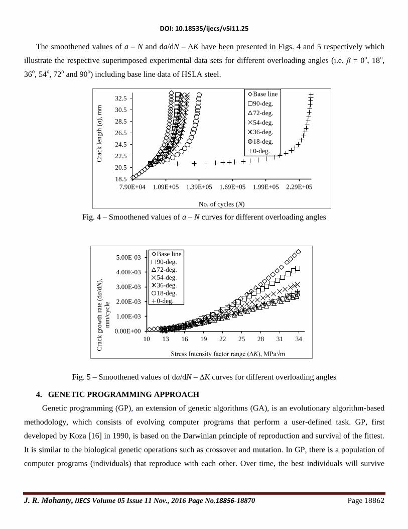
The smoothened values of a – N and da/dN – ΔK have been presented in Figs. 4 and 5 respectively which

illustrate the respective superimposed experimental data sets for different overloading angles (i.e. β = 0o, 18

o,

36o, 54

o, 72

o and 90

o) including base line data of HSLA steel.

Fig. 4 – Smoothened values of a – N curves for different overloading angles

Fig. 5 – Smoothened values of da/dN – ∆K curves for different overloading angles

4. GENETIC PROGRAMMING APPROACH

Genetic programming (GP), an extension of genetic algorithms (GA), is an evolutionary algorithm-based

methodology, which consists of evolving computer programs that perform a user-defined task. GP, first

developed by Koza [16] in 1990, is based on the Darwinian principle of reproduction and survival of the fittest.

It is similar to the biological genetic operations such as crossover and mutation. In GP, there is a population of

computer programs (individuals) that reproduce with each other. Over time, the best individuals will survive

DOI: 10.18535/ijecs/v5i11.25


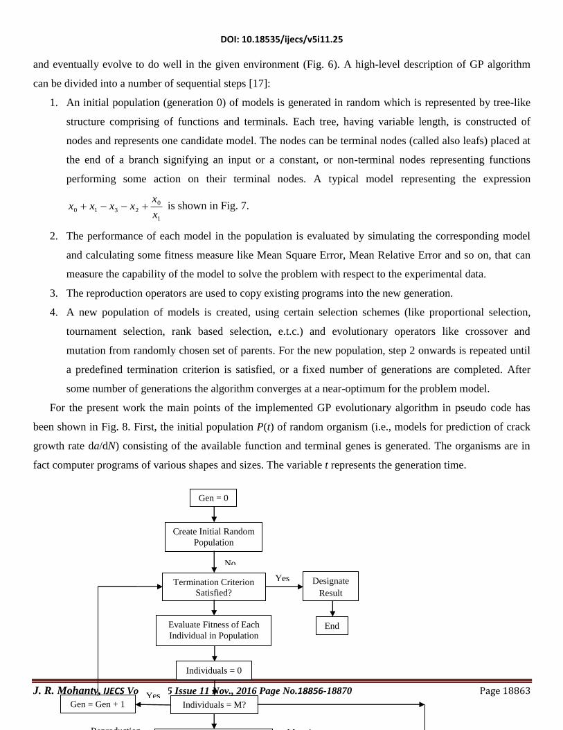
and eventually evolve to do well in the given environment (Fig. 6). A high-level description of GP algorithm

can be divided into a number of sequential steps [17]:

1. An initial population (generation 0) of models is generated in random which is represented by tree-like

structure comprising of functions and terminals. Each tree, having variable length, is constructed of

nodes and represents one candidate model. The nodes can be terminal nodes (called also leafs) placed at

the end of a branch signifying an input or a constant, or non-terminal nodes representing functions

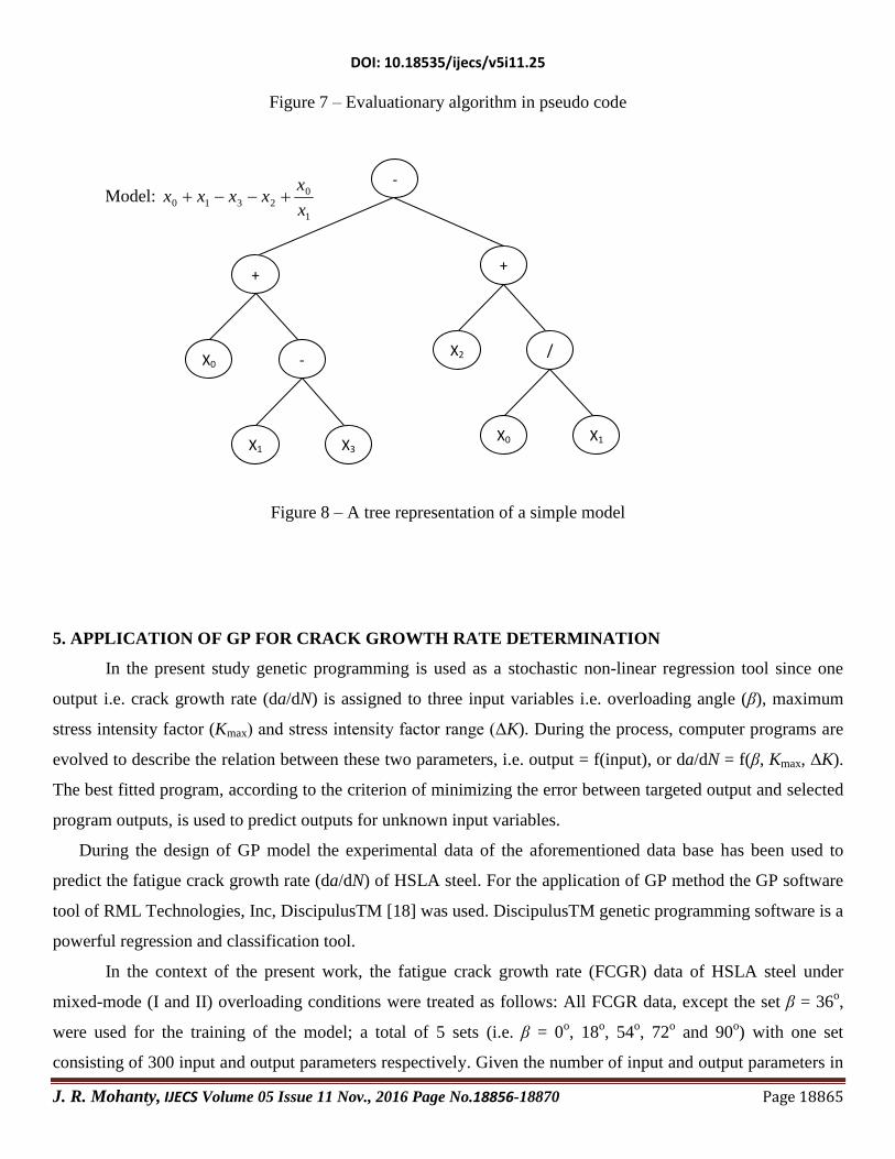
performing some action on their terminal nodes. A typical model representing the expression

1

0

2310x

xxxxx is shown in Fig. 7.

2. The performance of each model in the population is evaluated by simulating the corresponding model

and calculating some fitness measure like Mean Square Error, Mean Relative Error and so on, that can

measure the capability of the model to solve the problem with respect to the experimental data.

3. The reproduction operators are used to copy existing programs into the new generation.

4. A new population of models is created, using certain selection schemes (like proportional selection,

tournament selection, rank based selection, e.t.c.) and evolutionary operators like crossover and

mutation from randomly chosen set of parents. For the new population, step 2 onwards is repeated until

a predefined termination criterion is satisfied, or a fixed number of generations are completed. After

some number of generations the algorithm converges at a near-optimum for the problem model.

For the present work the main points of the implemented GP evolutionary algorithm in pseudo code has

been shown in Fig. 8. First, the initial population P(t) of random organism (i.e., models for prediction of crack

growth rate da/dN) consisting of the available function and terminal genes is generated. The organisms are in

fact computer programs of various shapes and sizes. The variable t represents the generation time.

No

Yes

Evaluate Fitness of Each

Individual in Population End

Gen = 0

Create Initial Random

Population

Termination Criterion

Satisfied?

Designate

Result

Individuals = M?

Individuals = 0

Gen = Gen + 1 Yes

Reproduction Mutation

DOI: 10.18535/ijecs/v5i11.25


Figure 6 – Genetic Programming Flow Chart [18]

t 0

t t+1

evolutionary algorithm

begin

initialize P(t)

evaluate P(t)

while (not termination_condition) do

begin

alter P(t) by applying genetic operators

evaluate P(t)

end

end

DOI: 10.18535/ijecs/v5i11.25


Figure 7 – Evaluationary algorithm in pseudo code

Figure 8 – A tree representation of a simple model

5. APPLICATION OF GP FOR CRACK GROWTH RATE DETERMINATION

In the present study genetic programming is used as a stochastic non-linear regression tool since one

output i.e. crack growth rate (da/dN) is assigned to three input variables i.e. overloading angle (β), maximum

stress intensity factor (Kmax) and stress intensity factor range (ΔK). During the process, computer programs are

evolved to describe the relation between these two parameters, i.e. output = f(input), or da/dN = f(β, Kmax, ΔK).

The best fitted program, according to the criterion of minimizing the error between targeted output and selected

program outputs, is used to predict outputs for unknown input variables.

During the design of GP model the experimental data of the aforementioned data base has been used to

predict the fatigue crack growth rate (da/dN) of HSLA steel. For the application of GP method the GP software

tool of RML Technologies, Inc, DiscipulusTM [18] was used. DiscipulusTM genetic programming software is a

powerful regression and classification tool.

In the context of the present work, the fatigue crack growth rate (FCGR) data of HSLA steel under

mixed-mode (I and II) overloading conditions were treated as follows: All FCGR data, except the set β = 36o,

were used for the training of the model; a total of 5 sets (i.e. β = 0o, 18

o, 54

o, 72

o and 90

o) with one set

consisting of 300 input and output parameters respectively. Given the number of input and output parameters in

+

X0 -

X1 X3

-

+

X2 /

X0

X1

Model:

1

0

2310x

xxxxx

DOI: 10.18535/ijecs/v5i11.25


the training set, the process is characterized as a non-linear stochastic regression analysis. During the training

phase the genetic programming tool established several relations (by regression analysis) in the form of

computer programs between the input and output variables. It is worthwhile to mention here that the proposed

GP formulation is valid for the ranges of training set as given in Table 3. Parameters of the GP models are

presented in Table 4. Using an iterative process the parameters of the established relations were adjusted in

order to minimize the error between targeted output and selected program outputs. The same model (the

selected evolved program) can be stored and potentially be used to predict other output values for a new applied

input data set (i.e. β = 36o).

Table 3 – Variables used in model construction

Code Input

variable

Range

Code Output

variable

Range

(Al-7020)

x1 Overload

angle (β)

0o – 90

o

(with a

diff. of 18o)

Crack

growth

rate

(da/dN)

6.37×10-5

–

2.58×10-3

x2 Maximum

stress

intensity

factor (Kmax)

13.35 –

37.22

x3 Stress

intensity

factor range

(∆K)

12.46 –

33.97

Table 4 – Parameters of GP model for the alloy

P1 Population size 1000

P2 Number of generations Between 100 to 7000

P3 Function set „-‟, „*‟, „power‟

P4 Probability of reproduction 0.1

P5 Probability of crossover 0.9

P6 Maximum depth of initial random organisms 4

P7 Maximum permissible depth organisms after crossover 10

6. RESULT AND DISCUSSION

In the present study, genetic programming was applied on the training data sets for modeling post

overload fatigue crack growth rates as described in the previous section. The data containing in the training file

were used for learning by applying the fitness function. Subsequently, the new inputs of the test data set (i.e. β =

DOI: 10.18535/ijecs/v5i11.25


0.00E+00

5.00E-04

1.00E-03

1.50E-03

2.00E-03

2.50E-03

3.00E-03

0.00E+005.00E-04 1.00E-03 1.50E-03 2.00E-03 2.50E-03 3.00E-03

Cra

ck g

row

th r

ate,

da

/dN

(G

P)

Crack growth rate, da/dN (Exp.)

Perfect fit

GP

36o) were fed to the trained GP model to predict the corresponding predicted outputs. The overall performances

of both sets were evaluated by the correlation coefficient (R) and mean squared error (MSE) given by:

22

expexp

1

expexp

predicteddNda

predicteddNda

erimentaldNda

erimentaldNda

predicteddNda

predicteddNda

m

i

erimentaldNda

erimentaldNda

R

(9)

nMSE

m

i

predicteddNda

erimentaldNda

1

exp

(10)

Where, erimentaldNda

exp and predicteddNda are the experimental and predicted crack growth rates,

erimentaldNda

exp

and predicteddNda

are their corresponding mean values and „n‟ is the number of observations.

The GP estimates are compared to the experimental data for training and testing sets. The statistical

performance of the GP model has been presented in Table 5.

Table 5 – Statistical results of GP for training and testing

Set MSE Corr. Coff. (R)

Train 2.4637 0.9856

Test 3.1587 0.9789

The training results proved that the proposed GP models have efficiently learned well the nonlinear

relationship between the input and output variables with high correlation (R = 0.9856) and relatively low error

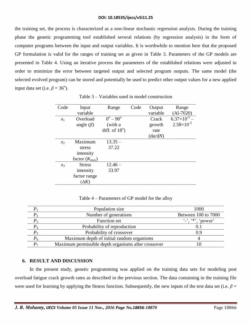
(MSE = 2.4637) values. Comparing the GP predictions with the experimental data for the test stage (Fig. 9)

demonstrates a high generalization capacity of the proposed model (R = 0.9789) and relatively low error (MSE

= 3.1587) values. All these findings show a successful performance of the GP model for estimating fatigue

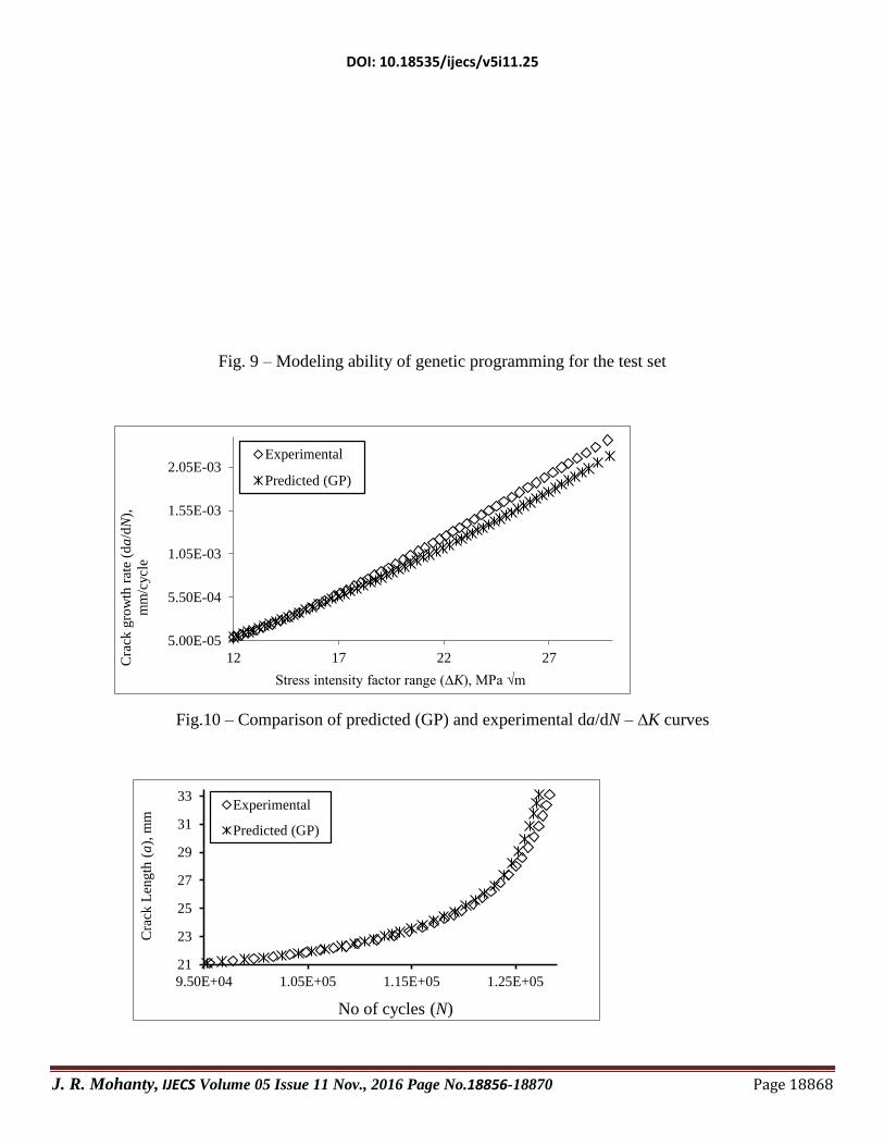
crack growth rates in training and testing stages. The testing results (da/dN vs. ∆K) have been illustrated in Fig.

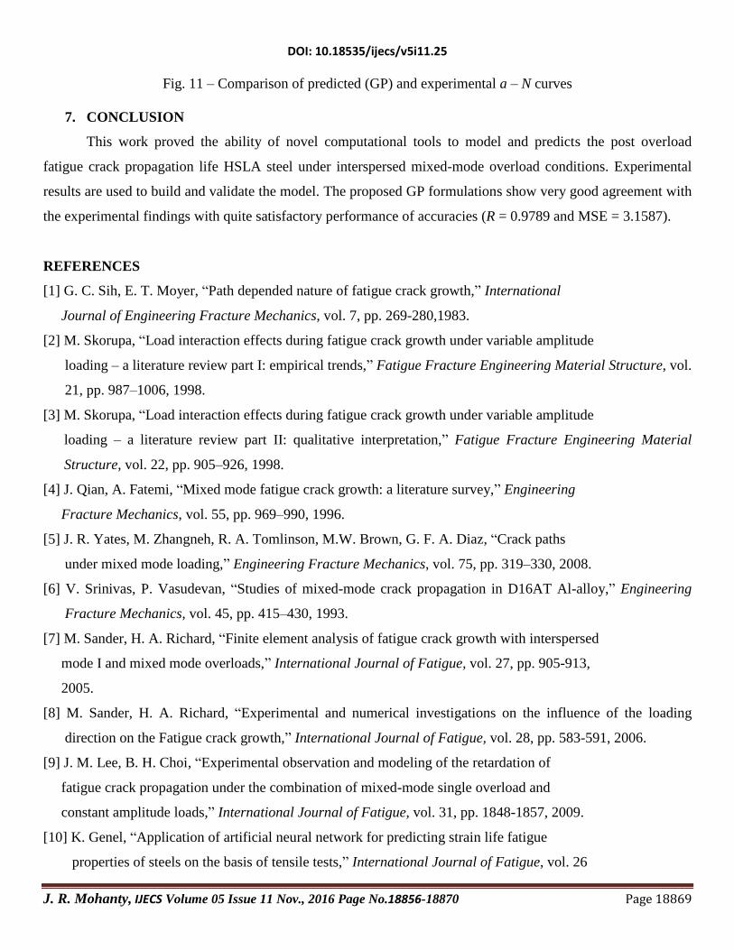
10 for HSLA steel. The numbers of cycles (i.e. post overload fatigue lives) were calculated from predicted and

experimental results in the excel sheet (Fig. 11) as per the following equation:

i

ii

i N

dNda

aaN

1

1 (11)

From the a – N plot it is observed that the post overload fatigue life (at β = 36o) of HSLA steel from GP model

is 127300 cycles with an error of – 0.787% in comparison to its experimental value which is 128310 cycles.

DOI: 10.18535/ijecs/v5i11.25


5.00E-05

5.50E-04

1.05E-03

1.55E-03

2.05E-03

12 17 22 27Cra

ck g

row

th r

ate

(da

/dN

),

mm

/cycle

Stress intensity factor range (∆K), MPa √m

Experimental

Predicted (GP)

21

23

25

27

29

31

33

9.50E+04 1.05E+05 1.15E+05 1.25E+05

Cra

ck L

ength

(a

), m

m

No of cycles (N)

Experimental

Predicted (GP)

Fig. 9 – Modeling ability of genetic programming for the test set

Fig.10 – Comparison of predicted (GP) and experimental da/dN – ∆K curves

DOI: 10.18535/ijecs/v5i11.25


Fig. 11 – Comparison of predicted (GP) and experimental a – N curves

7. CONCLUSION

This work proved the ability of novel computational tools to model and predicts the post overload

fatigue crack propagation life HSLA steel under interspersed mixed-mode overload conditions. Experimental

results are used to build and validate the model. The proposed GP formulations show very good agreement with

the experimental findings with quite satisfactory performance of accuracies (R = 0.9789 and MSE = 3.1587).

REFERENCES

[1] G. C. Sih, E. T. Moyer, “Path depended nature of fatigue crack growth,” International

Journal of Engineering Fracture Mechanics, vol. 7, pp. 269-280,1983.

[2] M. Skorupa, “Load interaction effects during fatigue crack growth under variable amplitude

loading – a literature review part I: empirical trends,” Fatigue Fracture Engineering Material Structure, vol.

21, pp. 987–1006, 1998.

[3] M. Skorupa, “Load interaction effects during fatigue crack growth under variable amplitude

loading – a literature review part II: qualitative interpretation,” Fatigue Fracture Engineering Material

Structure, vol. 22, pp. 905–926, 1998.

[4] J. Qian, A. Fatemi, “Mixed mode fatigue crack growth: a literature survey,” Engineering

Fracture Mechanics, vol. 55, pp. 969–990, 1996.

[5] J. R. Yates, M. Zhangneh, R. A. Tomlinson, M.W. Brown, G. F. A. Diaz, “Crack paths

under mixed mode loading,” Engineering Fracture Mechanics, vol. 75, pp. 319–330, 2008.

[6] V. Srinivas, P. Vasudevan, “Studies of mixed-mode crack propagation in D16AT Al-alloy,” Engineering

Fracture Mechanics, vol. 45, pp. 415–430, 1993.

[7] M. Sander, H. A. Richard, “Finite element analysis of fatigue crack growth with interspersed

mode I and mixed mode overloads,” International Journal of Fatigue, vol. 27, pp. 905-913,

2005.

[8] M. Sander, H. A. Richard, “Experimental and numerical investigations on the influence of the loading

direction on the Fatigue crack growth,” International Journal of Fatigue, vol. 28, pp. 583-591, 2006.

[9] J. M. Lee, B. H. Choi, “Experimental observation and modeling of the retardation of

fatigue crack propagation under the combination of mixed-mode single overload and

constant amplitude loads,” International Journal of Fatigue, vol. 31, pp. 1848-1857, 2009.

[10] K. Genel, “Application of artificial neural network for predicting strain life fatigue

properties of steels on the basis of tensile tests,” International Journal of Fatigue, vol. 26

DOI: 10.18535/ijecs/v5i11.25


pp. 1027-1035, 2004.

[11] A. Fotovati, T. Goswami, “Prediction of elevated temperature fatigue crack growth

rates in Ti-6Al-4V alloy – neural network approach,” Material Engineering Design, vol. 25

pp. 547-554, 2004.

[12] M. A. Jarrah, Y. H. Al-assaf, E. kadi, “Neuro-Fuzzy Modeling of Fatigue Life

Prediction of Unidirectional Glass Fiber/Epoxy Composite Laminates,” Journal of

Composite Material, 36, pp. 685-699, 2002.

[13] A. P. Vassilopoulos, E. F. Georgopoulos, T. Keller, “Comparison of genetic

programming with conventional methods for fatigue life modelling of FRP composite

materials,” International Journal of Fatigue, vol. 30, pp. 1634-1645, 2008.

[14] J. R. Mohanty, B. B. Verma, P. K. Ray, “Evaluation of overload-induced fatigue crack

growth retardation parameters using an exponential model,” Engineering Fracture Mechanics, vol. 75, pp.

3941–3951, 2008.

[15] J. R. Mohanty, B. B. Verma, P. K. Ray, “Determination of fatigue crack growth rate from experimental

data: A new approach,” International Journal of Microstructure & Material Properties, vol. 5, pp. 79–

87, 2010.

[16] J. R. Koza, “Genetic programming: on the programming of computers by means of natural

Selection,” MIT Press, London, 1992.

[17] K. M. Faraoun, A. Boukelif, “Genetic programming approach for multi-category pattern

classification applied to network intrusion detection,” International Journal of

Computational Intelligence & Application, vol. 5, no. 6, pp. 77–99, 2006.

[18] AIM Learning Technology, http://www.aimlearning.com.

Documents

Prediction of post overload fatigue crack growth life of …ijecs.in/issue/v5-i11/25 ijecs.pdfvariable amplitude loads, block loads etc. In real situations, ... different angles of