Predicting the Path of Technological Innovation: SAW vs ...gareth/research/MktSciSAW.pdf · Predicting the Path of Technological Innovation: SAW vs. Moore, Bass, Gompertz, and Kryder

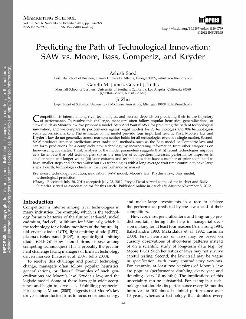
Vol. 31, No. 6, November–December 2012, pp. 964–979ISSN 0732-2399 (print) � ISSN 1526-548X (online) http://dx.doi.org/10.1287/mksc.1120.0739

© 2012 INFORMS

Predicting the Path of Technological Innovation:SAW vs. Moore, Bass, Gompertz, and Kryder

Ashish SoodGoizueta School of Business, Emory University, Atlanta, Georgia 30322, [email protected]

Gareth M. James, Gerard J. TellisMarshall School of Business, University of Southern California, Los Angeles, California 90089

{[email protected], [email protected]}

Ji ZhuDepartment of Statistics, University of Michigan, Ann Arbor, Michigan 48109, [email protected]

Competition is intense among rival technologies, and success depends on predicting their future trajectoryof performance. To resolve this challenge, managers often follow popular heuristics, generalizations, or

“laws” such as Moore’s law. We propose a model, Step And Wait (SAW), for predicting the path of technologicalinnovation, and we compare its performance against eight models for 25 technologies and 804 technologies-years across six markets. The estimates of the model provide four important results. First, Moore’s law andKryder’s law do not generalize across markets; neither holds for all technologies even in a single market. Second,SAW produces superior predictions over traditional methods, such as the Bass model or Gompertz law, andcan form predictions for a completely new technology by incorporating information from other categories ontime-varying covariates. Third, analysis of the model parameters suggests that (i) recent technologies improveat a faster rate than old technologies; (ii) as the number of competitors increases, performance improves insmaller steps and longer waits; (iii) later entrants and technologies that have a number of prior steps tend tohave smaller steps and shorter waits; but (iv) technologies with a long average wait time continue to have largesteps. Fourth, technologies cluster in their performance by market.

Key words : technology evolution; innovation; SAW model; Moore’s law; Kryder’s law; Bass model;technological prediction

History : Received: July 20, 2011; accepted: July 23, 2012; Preyas Desai served as the editor-in-chief and RajivSurendra served as associate editor for this article. Published online in Articles in Advance November 5, 2012.

IntroductionCompetition is intense among rival technologies inmany industries. For example, which is the technol-ogy for auto batteries of the future: lead–acid, nickelcadmium, fuel cell, or lithium ion? Similarly, which isthe technology for display monitors of the future: liq-uid crystal diode (LCD), light-emitting diode (LED),plasma display panel (PDP), or organic light-emittingdiode (OLED)? How should firms choose amongcompeting technologies? This is probably the preemi-nent challenge facing managers of firms in technologydriven markets (Hauser et al. 2007, Tellis 2008).

To resolve this challenge and predict technologychange, managers often follow popular heuristics,generalizations, or “laws.” Examples of such gen-eralizations are Moore’s law, Kryder’s law, and thelogistic model. Some of these laws gain wide accep-tance and begin to serve as self-fulfilling prophecies.For example, Moore (2003) suggests that Moore’s lawdrove semiconductor firms to focus enormous energy

and make large investments in a race to achievethe performance predicted by the law ahead of theircompetitors.

However, most generalizations and long-range pre-dictions fail, offering little help in managerial deci-sion making for at least four reasons (Armstrong 1984,Balachandra 1980, Makridakis et al. 1982, Tashman2000). First, heuristics or laws may be based oncursory observations of short-term patterns insteadof on a scientific study of long-term data (e.g., byMoore 1965). Such heuristics or laws may not survivecareful testing. Second, the law itself may be vaguein specification, with many contradictory versions.For example, at least two versions of Moore’s laware popular (performance doubling every year anddoubling every 18 months). The implications of thisuncertainty can be substantial. For example, a tech-nology that doubles its performance every 18 monthsimproves to 100 times its initial performance over10 years, whereas a technology that doubles every

964

INFORMS

holds

copyrightto

this

article

and

distrib

uted

this

copy

asa

courtesy

tothe

author(s).

Add

ition

alinform

ation,

includ

ingrig

htsan

dpe

rmission

policies,

isav

ailableat

http://journa

ls.in

form

s.org/.

Sood et al.: SAW vs. Moore, Bass, Gompertz, and KryderMarketing Science 31(6), pp. 964–979, © 2012 INFORMS 965

year improves to more than 1,000 times its initial per-formance in the same period. Third, the popularityof a law may encourage indiscriminate extension tomany fields, technologies, and industries. For exam-ple, Moore’s law has been claimed to apply to sev-eral metrics of technology performance, including thesize, cost, density, and speed of components in thesemiconductor industry, and many other technolo-gies besides semiconductors, such as biotechnology,nanotechnology, and genomics (Edwards 2008, Wolff2004). In fact, Moore (1995, p. 1) suggests that thelaw has come to refer to “almost anything related tothe semiconductor industry that when plotted on asemi-log paper approximates a straight line.” Notethat without the exact specification of the slope ofthe straight line, the law is intrinsically flexible andsusceptible to hindsight bias. Fourth, prior researchis inconclusive on whether the path of technologyevolution is smooth or irregular, suggesting that adata-driven approach is better for prediction thandependence on generalized heuristics. All four rea-sons suggest the need for a better model for pre-dicting the path of technology evolution. The currentresearch addresses these limitations in the literatureon technology evolution and addresses these researchquestions:

• How valid are the traditional laws and modelsfor describing technology evolution?

• Which model can best predict the path of tech-nological innovation?

• What are the key drivers of technologyevolution?

To address these questions, we propose a newmodel called Step And Wait (SAW) and test itagainst extant models for 25 technologies and 804technologies-years across six markets for over severaldecades. We make four contributions to the currentliterature. First, we propose a model to predict theevolution of technological performance that providesbetter predictions than traditional models. Such pre-diction allows both marketing and technology man-agers to identify dimensions on which to focus theirnew product design efforts. Second, the proposedmodel allows for predicting the path of an entirelynew technology based on the similarity of its char-acteristics to those of prior technologies. Third, theexercise enables us to test the validity and generaliz-ability of some popular laws about technology evo-lution. Fourth, we identify key drivers of technologyevolution.

The next five sections present the theory, hypothe-ses, models, method, and results. The last section dis-cusses the findings, implications, and limitations ofthe research.

Theory of Technology EvolutionTechnology evolution is the improvement in the per-formance of a technology over time. We are inter-ested in a better understanding of the path of suchimprovement. Prior literature has debated the shapeof the path (whether smooth or discontinuous) andthe drivers of the path (explanatory variables thatinfluence its course). We cover both of these topicsnext.

Shape of PathPrior literature suggests both smooth change throughincremental improvements occurring frequently(Basalla 1988, Dosi 1982) and nonsmooth changethrough relatively stable periods of smooth changepunctuated with discontinuous steps of big changes(D’Aveni 1994, Eldredge and Gould 1972, Tushmanand Anderson 1986).

Proponents of smooth and incremental technolog-ical change (e.g., Basalla 1988) argue that technol-ogy evolution is a process of continual improvementin performance of a technology through novelrecombination and synthesis of existing technologies(Henderson and Clark 1990). These researchers sug-gest that changes in technology performance are aresult of changes in a number of domains, includ-ing beliefs, values, culture, technology, operating rou-tines, organizational structure, resources, and corecompetencies (Gersick 1991, Tushman and Romanelli1985, Wollin 1999). Invention is a social process thatrests on the accumulation of many minor improve-ments, not the heroic efforts of a few geniuses (Basalla1988, Dosi 1982).

Proponents of irregular change (e.g., Adner 2002,Eldredge and Gould 1972, Tushman and Anderson1986) suggest that technologies improve througheras of smooth change punctuated by discontinu-ous shifts. Products that draw upon fundamentallynew technologies enter an industry and create fer-ment till the emergence of dominant designs (Nelsonand Winter 1977, Utterback and Abernathy 1975).After a dominant design is established, firms focusmore on process innovations than on product inno-vations (Henderson and Clark 1990). Jumps in prod-uct performance could occur from both product andprocess innovation related to the focal technology.Tushman and Anderson (1986) explain the discontinu-ous nature of technological change through two typesof change—competence enhancing and competencedestroying. Levinthal (1998) extends the concept ofnatural speciation (Eldredge and Gould 1972) to tech-nology speciation. Substantial improvements in per-formance occur because a shift of a technology fromone domain to another alters the relative preferencefor attributes, demands different price/performance

INFORMS

holds

copyrightto

this

article

and

distrib

uted

this

copy

asa

courtesy

tothe

author(s).

Add

ition

alinform

ation,

includ

ingrig

htsan

dpe

rmission

policies,

isav

ailableat

http://journa

ls.in

form

s.org/.

Sood et al.: SAW vs. Moore, Bass, Gompertz, and Kryder966 Marketing Science 31(6), pp. 964–979, © 2012 INFORMS

ratio for older attributes, and often releases substan-tially higher resources for research and development(R&D) (Levinthal 1998). This shift may be due to(1) changes in problem-solving heuristics; (2) fusionwith other domains; and (3) other technological,social, or economic aspects. Such shifts provide accessto new customers, resources, and performance met-rics (Adner 2002). As a result, the technology exhibitssharp steps in performance.

In summary, even though debate in prior researchis inconclusive as to whether technology evolution issmooth or irregular, the question remains importantto managers. Thus, good forecasting capabilities mayspell the difference between success and failure in themarket.

Drivers of Path of Technological ChangeOur review of the theory in this area suggests fourcovariates that could drive the path of technologicalchange. We discuss the role of each of these covariatesnext.1

Year of Introduction. This covariate reflects thenewness of the technology. We hypothesize that newtechnologies improve in larger and more frequentsteps than old technologies as a result of the improve-ment in the supporting environment for innovationin recent years. In particular, improvements in sup-porting environment are characterized by (1) highertotal R&D expenditures, (2) more researchers devotedto technology research, (3) use of better tools, (4) bet-ter laboratories, (5) better communication of research,and (6) more countries focused on research.

In addition, the pace of improvement in new tech-nologies may occur more frequently and in largersteps than old technologies for three reasons. (1) Aftera period of rapid improvement in performance, oldtechnologies may reach a period of maturity (Foster1986, Brown 1992, Chandy and Tellis 2000, Soodand Tellis 2011). Foster (1986) suggests that matura-tion may be an innate feature of each technology.Sahal (1981) proposes that maturity occurs becauseof limits of scale or system complexity. Fleming(2001) suggests that old technologies reach recombi-nant exhaustion and improvements become smaller.And Golder and Tellis (2004) suggest that matura-tion can result from abandonment following a cas-cade. (2) Newer technologies attract the interest offirms. Market power acquired from successful inno-vation in the old technologies spurs greater inventiveactivity in new technologies. They seem mysteriousyet promise huge benefits. As such, they attract.

1 Other factors (e.g., market size, technological sophistication) mayalso affect the evolution but have not been included in the analysisbecause of a lack of reliable data on these variables. We thank ananonymous reviewer for suggesting these.

(3) New technologies also introduce new performancedimensions unrelated to those offered by old tech-nologies. For example, before the advent of LCD mon-itors, firms making CRT (cathode ray tube) monitorscompeted mainly on higher screen resolution. LCDmonitors promised compactness as a new perfor-mance dimension. Old technologies strive to competeas customer demand for these dimensions increases.This slows performance improvements on the exist-ing dimension. Thus, we hypothesize the following.

Hypothesis 1 (H1). Performance of more recent tech-nologies increases in (1) larger steps and (2) more frequentsteps (shorter wait times).

Order of Entry. After controlling for the basic effectof calendar time, the order of entry of a technol-ogy in a particular market could affect its improve-ment. We need to emphasize that the time effectprobably holds for large time spans such as decades.The order of entry works for small time spans suchas a few years within a market, within which onetechnology follows another pretty rapidly. We iden-tify two rival theories: preferential attraction versusprecommitment.

The preferential attraction theory holds that theearlier technology gets more (or better, and initially,all) of the limited set of resources (dollars, locations,and researchers) than those technologies that follow.Risk aversion of investors and researchers preventsthem from investing in new technologies. Prior lit-erature also suggests that pioneers outperform laterentrants (Lambkin 1988, Urban et al. 1986). If thisline of reasoning is valid, the earlier technology willhave larger and more frequent improvements in per-formance than later technologies within the samemarket. The above argument leads to the followinghypothesis.

Hypothesis 2A (H2A). Technologies entering earlierimprove with (1) larger steps and (2) more frequent steps(shorter wait times) than later technologies within the samemarket.

The precommitment argument suggests that theearlier technology enters in an environment with lessinformation about potential markets, dimensions ofperformance, and available resources than the tech-nology that enters later. Thus, the earlier technol-ogy precommits to an evolutionary path that maynot be the most efficient or effective. The later tech-nology enters in an environment with greater infor-mation about markets, technologies, and resources,and it chooses a more efficient and productive evo-lutionary path (Golder and Tellis 1993). The glamourof the “new” may also result in suppliers switchingresources from the old to the new. Thus, a technologyentering a market later will have more resources and

INFORMS

holds

copyrightto

this

article

and

distrib

uted

this

copy

asa

courtesy

tothe

author(s).

Add

ition

alinform

ation,

includ

ingrig

htsan

dpe

rmission

policies,

isav

ailableat

http://journa

ls.in

form

s.org/.


more researchers working on it than an older tech-nology. This will result in more frequent but smallersteps in performance. The above argument leads tothe following rival hypothesis.

Hypothesis 2B (H2B). Technologies entering laterimprove with (1) smaller steps and (2) more frequent steps(shorter wait times) than earlier technologies to a market.

Number of Competing Technologies. Controllingfor the effects above, how does improvement relate tothe number of competing technologies? We proposetwo rival theories: competition for limited resourcesor competition spurring breakthroughs.

The limitation of resources theory is that in anymarket the amount of dollars, researchers, and labsis relatively fixed in the immediate short term. Thusas the number of competing technologies increases,each resource becomes more scarce. This divisionof resources results in less frequent breakthroughsand therefore less frequent increases in performance.More competition leads firms to become more riskaverse and focus on cost management instead ofrisky and costly product improvement. Firms gener-ally achieve these objectives by prioritizing processinnovation over product innovation (Scherer and Ross1990). Thus, as the number of competitors increases,improvements in performance are slower.

The rival theory is of competition spurring break-throughs. This phenomenon could occur for severalreasons. First, each technology is supported by aunique set of researchers with their own egos, train-ing, reputation, and emotional attachment. As thenumber of competing technologies increases, theirsupporters work harder to promote their own tech-nologies and create improvements in performance.It is also possible that more firms enter a marketbecause (a) there is demand or (b) because they thinkit is relatively easy to improve existing products (tech-nologies). In other words, if (b) is true, there are moreentrants because technological progress is likely to befast.2 As a result, the number of improvements in per-formance increases with the number of competitiontechnologies in a market. Second, Rosenberg (1969)refers to the phenomenon of compulsive sequence,where a breakthrough in one area typically gener-ates new technical problems, creating imbalances thatrequire further innovative effort to fully realize thebenefits of the initial breakthrough. For example, thedevelopment of high-speed steel improved cuttingtools and stimulated the development of sturdier andmore adaptable machines to drive them (Rosenberg1969). Third, new technologies may set up additionalopportunities in new niches even for old technolo-gies. Fourth, prior research suggests that a firm’s

2 We thank an anonymous reviewer for suggesting this possibility.

returns from innovation at the margin are larger inan oligopolistic versus a monopolistic environment(Fellner 1961, Arrow 1962, Scherer 1967). Thus, morecompetition generates more funds to support inno-vation and faster product improvements. All thesereasons suggest that an increase in the number ofcompetitors will increase the number of improve-ments in technology performance. Thus, we can pro-pose the following rival hypotheses.

Hypothesis 3A (H3A). As the number of competi-tors increases, performance of technologies increases in(1) smaller steps and (2) longer wait times.

Hypothesis 3B (H3B). As the number of competi-tors increases, performance of technologies increases in(1) larger steps and (2) shorter wait times.

Technology Characteristics. We include two covar-iates to capture technology characteristics—the num-ber of prior steps and average prior wait time.Together, the two covariates capture unique pat-terns of technological improvement for a technologywithin its unique technological paradigm (Nelson andWinter 1982, Dosi 1982). A technological paradigm isthe common platform on which scientists and tech-nologists agree to do research and explain the speedand pattern of technological advancement. For exam-ple, for the past 30 years, firms in the magnetic stor-age industry pursued higher areal density as a goalto solve design problems and achieve higher produc-tivity. This common understanding led firms to raceto introduce improvements in areal density ahead ofother firms. In such an urgency, firms may not delayinvestments in R&D and frequently introduce prod-ucts with improvements.

In technologies where such a paradigm emerges,a technology evolves with a large number of steps.However, these steps are small and frequent. Firmstake advantage of interdependencies with compo-nents and advancements in other fields. For example,improvements in the areal density of magnetic storagehave been driven in part by advancements in otherrelated disciplines such as semiconductor, fiber optic,and microelectronics.

In the absence of a dominant technological para-digm, firms’ efforts scatter in diverse directions. R&Defforts may be targeted toward improvements ondiverse performance metrics leading to little synergyacross firms’ efforts and to fewer steps. Also, com-peting firms within an industry may wait to intro-duce products to optimize commercialization costs.As a result, there are few steps with long wait times.Longer average wait times also provide firms moretime to develop better products. This results in tech-nological progress with large step sizes and long waittimes. Thus, the technological paradigm theory sug-gests the following two hypotheses.

INFORMS

holds

copyrightto

this

article

and

distrib

uted

this

copy

asa

courtesy

tothe

author(s).

Add

ition

alinform

ation,

includ

ingrig

htsan

dpe

rmission

policies,

isav

ailableat

http://journa

ls.in

form

s.org/.


Hypothesis 4 (H4). Technologies with a large numberof prior steps have (1) small current steps and (2) a shortercurrent wait time.

Hypothesis 5 (H5). Technologies with long averageprior wait times have (1) large current steps and (2) a longcurrent wait time.

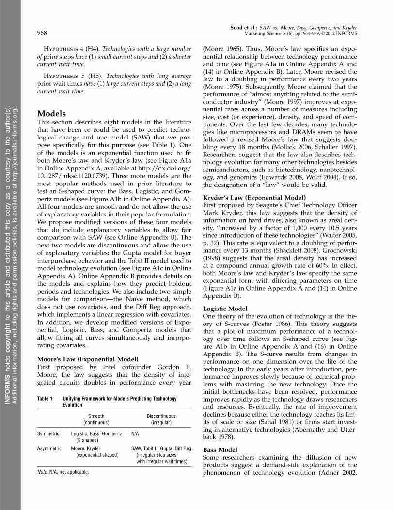
ModelsThis section describes eight models in the literaturethat have been or could be used to predict techno-logical change and one model (SAW) that we pro-pose specifically for this purpose (see Table 1). Oneof the models is an exponential function used to fitboth Moore’s law and Kryder’s law (see Figure A1ain Online Appendix A, available at http://dx.doi.org/10.1287/mksc.1120.0739). Three more models are themost popular methods used in prior literature totest an S-shaped curve: the Bass, Logistic, and Gom-pertz models (see Figure A1b in Online Appendix A).All four models are smooth and do not allow the useof explanatory variables in their popular formulation.We propose modified versions of these four modelsthat do include explanatory variables to allow faircomparison with SAW (see Online Appendix B). Thenext two models are discontinuous and allow the useof explanatory variables: the Gupta model for buyerinterpurchase behavior and the Tobit II model used tomodel technology evolution (see Figure A1c in OnlineAppendix A). Online Appendix B provides details onthe models and explains how they predict holdoutperiods and technologies. We also include two simplemodels for comparison—the Naïve method, whichdoes not use covariates, and the Diff Reg approach,which implements a linear regression with covariates.In addition, we develop modified versions of Expo-nential, Logistic, Bass, and Gompertz models thatallow fitting all curves simultaneously and incorpo-rating covariates.

Moore’s Law (Exponential Model)First proposed by Intel cofounder Gordon E.Moore, the law suggests that the density of inte-grated circuits doubles in performance every year

Table 1 Unifying Framework for Models Predicting TechnologyEvolution

Smooth Discontinuous(continuous) (irregular)

Symmetric Logistic, Bass, Gompertz N/A(S shaped)

Asymmetric Moore, Kryder SAW, Tobit II, Gupta, Diff Reg(exponential shaped) (irregular step sizes

with irregular wait times)

Note. N/A, not applicable.

(Moore 1965). Thus, Moore’s law specifies an expo-nential relationship between technology performanceand time (see Figure A1a in Online Appendix A and(14) in Online Appendix B). Later, Moore revised thelaw to a doubling in performance every two years(Moore 1975). Subsequently, Moore claimed that theperformance of “almost anything related to the semi-conductor industry” (Moore 1997) improves at expo-nential rates across a number of measures includingsize, cost (or experience), density, and speed of com-ponents. Over the last few decades, many technolo-gies like microprocessors and DRAMs seem to havefollowed a revised Moore’s law that suggests dou-bling every 18 months (Mollick 2006, Schaller 1997).Researchers suggest that the law also describes tech-nology evolution for many other technologies besidessemiconductors, such as biotechnology, nanotechnol-ogy, and genomics (Edwards 2008, Wolff 2004). If so,the designation of a “law” would be valid.

Kryder’s Law (Exponential Model)First proposed by Seagate’s Chief Technology OfficerMark Kryder, this law suggests that the density ofinformation on hard drives, also known as areal den-sity, “increased by a factor of 1,000 every 10.5 yearssince introduction of these technologies” (Walter 2005,p. 32). This rate is equivalent to a doubling of perfor-mance every 13 months (Shacklett 2008). Grochowski(1998) suggests that the areal density has increasedat a compound annual growth rate of 60%. In effect,both Moore’s law and Kryder’s law specify the sameexponential form with differing parameters on time(Figure A1a in Online Appendix A and (14) in OnlineAppendix B).

Logistic ModelOne theory of the evolution of technology is the the-ory of S-curves (Foster 1986). This theory suggeststhat a plot of maximum performance of a technol-ogy over time follows an S-shaped curve (see Fig-ure A1b in Online Appendix A and (16) in OnlineAppendix B). The S-curve results from changes inperformance on one dimension over the life of thetechnology. In the early years after introduction, per-formance improves slowly because of technical prob-lems with mastering the new technology. Once theinitial bottlenecks have been resolved, performanceimproves rapidly as the technology draws researchersand resources. Eventually, the rate of improvementdeclines because either the technology reaches its lim-its of scale or size (Sahal 1981) or firms start invest-ing in alternative technologies (Abernathy and Utter-back 1978).

Bass ModelSome researchers examining the diffusion of newproducts suggest a demand-side explanation of thephenomenon of technology evolution (Adner 2002,

INFORMS

holds

copyrightto

this

article

and

distrib

uted

this

copy

asa

courtesy

tothe

author(s).

Add

ition

alinform

ation,

includ

ingrig

htsan

dpe

rmission

policies,

isav

ailableat

http://journa

ls.in

form

s.org/.


Bass 1969, Rogers 1962, Young and Ord 1989,Young 1993). These researchers suggest that con-sumers adopt a new product based on spontaneousinnovation driven by word-of-mouth diffusion. Thisprocess carves a typical S-shape of sales of a newproduct (Sood et al. 2009) (see Figure A1b in OnlineAppendix A and (18) in Online Appendix B). Thedemand for the new product drives the evolution of anew technology, on which the new product is based,and it also follows an S-curve.

Gompertz’s ModelGompertz’s law was first proposed by British actu-ary Benjamin Gompertz for use in demographic stud-ies and suggests that the rate of human mortalityincreases exponentially with age (Gompertz 1825).In the current context, Gompertz’s law states thatthe maturity and exit of old technologies pave theway for the new technologies and drive technologyevolution (Young and Ord 1989). The rate of changein the performance of a technology increases at anexponential rate, tracing a sigmoid double exponen-tial S-shaped path over the life of the technology fromits introduction to its maturity (see Figure A1b inOnline Appendix A and (21) in Online Appendix B).Gompertz’s law has been used extensively in priorliterature to describe technology evolution becauseit produces S-shaped curves that describe the dif-ferent phases of evolution—acceleration, inflection,and deceleration of growth over time (Martino 2003;Meade and Islam 1995, 1998, 2006; Young and Ord1989). The different S-shaped curves have differentimplications in symmetry around the relative locationof the inflection point. These differences may influ-ence the power of these laws to predict technologyevolution.

Gupta ModelThe model of Gupta (1988) is a well-known and pop-ular approach for modeling consumer purchase deci-sions. This model consists of three separate stages:brand choice (for modeling the probability of pur-chasing a particular brand), interpurchase time (formodeling time until purchase), and purchase quan-tity (for modeling the amount of goods purchased).We use two stages of this model—interpurchase timeand quantity—to model the wait time and size of step,respectively. This model provides a natural approachfor predicting the discontinuous nature of technologyevolution (see Figure A1c in Online Appendix A and(23) and (24) in Online Appendix B).

Tobit II ModelThe Tobit II models the evolution of technologiesas a series of step functions with random improve-ments over irregular periods of time (see Figure A1c

in Online Appendix A and (25) and (26) in OnlineAppendix B). The model includes a latent variablethat represents the probability of a step as a functionof explanatory variables.

Simple Models: Naïve and Diff RegWe also include two simple alternatives. The firstmethod, Naïve, models technology curves as constantin the holdout period. In other words, we assumethat the curve for each technology is horizontal;i.e., if our last observation in the estimation sampleis �, we predict � for the entire holdout period. Thesecond method, Diff Reg, performs a single linearregression on all technologies simultaneously using atechnology-specific indicator variable and the covari-ates from the previous section as the independentvariables. The indicator variable is modeled as a ran-dom effect. The change in (log) technology perfor-mance between two successive periods is used as thedependent variable. So, for example, if a technologyremained constant between two periods, we set Y = 0for the response. After fitting the linear regressionmodel, we use the covariates of a technology to pre-dict its change in each time period and hence theentire trajectory.

SAW ModelWe propose a new approach that models technolo-gies as exhibiting periods of constant performancefollowed by discontinuous steps (see Figure A1c inOnline Appendix A). We call this model Step AndWait because it predicts steps in performance fol-lowed by a flat “waiting” period before the next step.Hence, it is in line with the theory that technologiesevolve according to irregular change. Our motivationin proposing SAW is to test whether such a discon-tinuous model could better predict the evolution ofa technology. SAW works by modeling the improve-ment in performance using the Step submodel and thetime between changes in performance using the Waitsubmodel. We describe the specification and predictionof SAW here and the fitting in Online Appendix C.

Specification. Let Jij and tij respectively representthe size of and the duration until the jth step fortechnology i. Let Tij represent the time betweenthe (j − 1)th and jth steps for technology i, sotij = ti4j−15 + Tij . SAW uses two submodels—the Stepsubmodel and the Wait submodel.

The Step submodel uses a hierarchical approach toestimate the size of the jth step for the ith technology,Jij , as a function of three quantities, M , �i1 and �ij , asfollows:

Jij ∼ Gamma4M1�i�ij51 (1)

�−1i ∼ Gamma4�1�51 (2)

�ij = exp4rTij +�1Yij1 + · · · +�qYijq51 (3)

INFORMS

holds

copyrightto

this

article

and

distrib

uted

this

copy

asa

courtesy

tothe

author(s).

Add

ition

alinform

ation,

includ

ingrig

htsan

dpe

rmission

policies,

isav

ailableat

http://journa

ls.in

form

s.org/.


where Yijk represents the value of the kth covariatefor technology i, at time tij , that is used to predictthe size of the step Jij . In this formulation, �, �, M ,r , and �11 0 0 0 1�q are parameters to be estimated fromthe data. The parameter M is a global value that con-tributes to the average step size for all technologies.The value of r controls the level and type of correla-tion between the step at time j , Jij , and the wait untilthis step, Tij . For r > 0, increased wait times implylarger steps. The term �ij is a function of the variouscovariates, such as the last wait time.

The random effect term, �i, is unique to each tech-nology and reflects its typical step size. SAW buildsstrength across all the data by estimating �i usingboth the previously observed step sizes for the ithtechnology and the typical step sizes of the other tech-nologies. Modeling �i as a random effect allows usto borrow strength across multiple technologies byassuming that the �i for each technology is drawnfrom a common distribution.

In theory, one could model Jij or �i as com-ing from a variety of distributions. However, theGamma distribution has the following advantages.(a) It is extremely flexible (it can model the mem-oryless exponential and the chi-square distributions,and it provides good approximations to Normal andt-distributions). (b) Using a Gamma allows us to cal-culate an exact likelihood function for the Step andWait submodels, which, in turn, provides a relativelysimple way of fitting the models by computing themaximum likelihood estimates. For a given �i, theexpected step size is a function of the covariates Yijk,the wait time Tij , and �i:

E4Jij ��i5 = M�i�ij

= M�i exp4rTij +�1Yij1 + · · · +�qYijq50

Hence, a technology with a small �i will tend tohave small step sizes, and vice versa, but this effectcan be moderated by the observed covariates (e.g.,a large investment in research and development attime tij5 through the parameter �ij . Since E4�−1

i 5 =

��, � and � provide information about the typicalstep size over all technologies. However, the indi-vidual covariates for each technology will also affectthe step size. The coefficients �11 0 0 0 1�q dictate therelationship between the covariates and the step size;for example, a positive value for �k indicates thatincreases in the kth covariate are associated withlarger step sizes, whereas �k = 0 would suggest nosuch relationship.

The Wait submodel works in a similar fashion, esti-mating the wait time until the (j + 1)th step for tech-nology i, Ti1 4j+15, as a function of three quantities,�i1�ij , and K, as follows:

Tij ∼ Gamma4K1�i�i4j−1551 (4)

�−1i ∼ Gamma4�1�51 (5)

�ij = exp4sJij +�1Xij1 + · · · +�pXijp51 (6)

where Xijk represents the value of the kth covariateused to predict Tij for technology i at time tij and K, �,�, �, s, and �11 0 0 0 1�p are parameters. The parameterK is a global value that contributes to the average waittime for all technologies, and s controls the correlationbetween the jth step, Jij , and the wait time until the(j+1)th step. A positive value of s implies longer waittimes after larger steps. The term �ij is a function ofthe various covariates for technology i (including thestep size Jij5 at time tij .

The random effect, �i, is unique to each technol-ogy and reflects its typical wait between steps. Again,SAW builds strength across all the data by estimat-ing �i using both the previously observed wait timesfor the ith technology and the typical wait times ofthe other technologies. For a given �i, the expectedwait until the next step is a function of the covariatesXijk1K, and �i:

E4Ti4j+15 � �i5

=K�i�4ij5 =K�i exp4sJij +�1Xij1 + · · · +�pXijp50

Hence, a technology with a small �i will tend to haveshort time periods between steps, and vice versa, butthis effect can be moderated by the observed covari-ates at time tij through the parameter �ij . For example,a technology may have a large �i and hence typi-cally experience long waits between steps, but at agiven time, this might be moderated by a changein the number of competing technologies, resultingin a small �ij and, hence, a smaller wait time. Theexpected value of �−1

i is ��. So � and � provideinformation about the typical wait time over all tech-nologies. However, the individual covariates for eachtechnology also affect the wait time. The coefficients�11 0 0 0 1�p dictate the relationship between the covari-ates and the wait time. For example, a positive valuefor �k indicates that increases in the kth covariateare associated with a longer wait, whereas �k = 0suggests no relationship between the kth covari-ate and the wait time. Because the covariates canchange over time, the typical Tij may increase ordecrease.

Predictions. Suppose for a given technology i weobserve ni steps, Ji ¢ = 4Ji11 0 0 0 1 Jini 5 with wait timesTi ¢ = 4Ti11 0 0 0 1 Tini 5. Note that ti0 represents the timeof introduction. So Ti1 corresponds to the durationfrom the introduction of a technology until the firststep, and Ji1 is the size of the first step. Then natu-ral estimates for the size of the next step, Ji4n1+15, andthe wait until the next step, Ti4ni+15, are E4Ji4n1+15 � Ji ¢5and E4Ti4ni+15 � Ti ¢5. Using the Step submodel given by

INFORMS

holds

copyrightto

this

article

and

distrib

uted

this

copy

asa

courtesy

tothe

author(s).

Add

ition

alinform

ation,

includ

ingrig

htsan

dpe

rmission

policies,

isav

ailableat

http://journa

ls.in

form

s.org/.


Equations (1)–(3), by the law of iterated expectationsand the fact that J �� has a gamma distribution,

E4Ji4ni+15 � Ji ¢5 = E4E4Ji4ni+15 ��i5 � Ji ¢5

= E4M�i4ni+15�i � Ji ¢5=M�i4ni+15E4�i � Ji ¢50

To compute the final expectation we need to derivethe expected value of � � J . The distribution of �−1

conditional on J ¢ is given by

f 4�−1� J ¢5∝f 4J ¢ ��−15f 4�−15

=

( ni∏

j=1

4�i�ij5−M JM−1

ij exp(

−�−1i

ni∑

j=1

Jij�−1ij

)

�−��−4�−15i

·exp4−�−1i /�5

)

·4â4M5niâ4�55−1

∝�−4Mni+�−15i exp

(

−�−1i

(

1�

+

ni∑

j=1

Jij�−1ij

))

0

Hence,

�−1i � J ¢ ∼ Gamma

(

Mni +�11

�−1 +∑ni

j=1 Jij�−1ij

)

1

but the expected value of the inverse of aGamma(�1�5 random variable is equal to 1/4�4�− 155.Therefore,

E4�i � Ji ¢5=�−1 +

∑nij=1 Jij�

−1ij

Mni +�− 11

and the expected size of the next step conditional onprevious steps is

E4Ji4ni+15 � Ji ¢5=M�i4ni+15

�−1+∑ni

j=1 Jij�−1ij

Mni +�− 10 (7)

Similarly, using the Wait submodel given by Equa-tions (4)–(6), the expected wait time until the next stepconditional on previous steps is (derivation is identi-cal to that for (7))

E4Ti4ni+15 � Ti ¢5 = K�iniE4�i � Ti ¢5

= K�ini

�−1 +∑ni

j=1 �−1i4j−15Tij

Kni +�− 10 (8)

From Equation (8), we can predict that the next stepin technology i will occur at time

ti4ni+15 = tini +E4Ti4ni+15 � Ti ¢5

= tini +K�ini

�−1 +∑ni

j=1 �−1i4j−15Tij

Kni +�− 11

the following step at time

ti4ni+25 = ti4ni+15 +K�i4ni+15

�−1 +∑ni

j=1 �−1i4j−15Tij

Kni +�− 11

and so on.

Together, Equations (7) and (8) can be used to pre-dict the entire remaining trajectory. Note that thisapproach will work even for a curve for which wehave no data. SAW can be used to estimate the size ofthe first step and the duration until the first step afterthe introduction of a new technology. In this case,ni = 0; so Equations (7) and (8) simplify as

E4Ti15=K�i0�−1

�− 11 (9)

E4Ji15=M�i1�−1

�− 10 (10)

Thus, given estimates for �i, �ij , �i, K, M , and�ij , one can predict the evolution of a technology asfar into the future as desired by combining the pre-dicted wait time (K�i�ij5 with the predicted step size(M�i�ij5.

Connections to Renewal-Reward Process. OurSAW model has similarities to a renewal-reward pro-cess (see Cox 1970). In particular, for fixed valuesof �i and �i, SAW fits a separate nonhomogeneousRRP to each technology. The nonhomogeneous com-ponent is introduced by virtue of the time-varyingcovariates. However, although conditional on �i and�i, each technology is independent, so these parame-ters are unobserved in practice. Thus SAW models theprocesses (technologies) as unconditionally related viathe Gamma distributions given by (2) and (5). In thissense, SAW can be considered a generalization of astandard renewal-reward process because it is build-ing strength across the technologies by jointly model-ing a series of related processes.

Extensions of the Exponential, Logistic, Bass,and Gompertz Models. In their standard forms, theExponential, Logistic, Bass, and Gompertz modelsall fit individually to a single technology and donot incorporate covariates in their specification. Thisspecification places them at a potential disadvantagerelative to SAW, which both utilizes the covariateinformation and builds strength across technologiesby fitting all curves simultaneously. To ensure a faircomparison, we fit modified versions of these meth-ods. In particular, we implemented two new versionsof each approach.

In the first implementation, we used a nonlin-ear mixed effects model (Pinheiro and Bates 2000),which fitted the standard functional forms of eachmethod but modeled the various parameters as ran-dom effects coming from a Gaussian distribution. Theparameters for the Gaussian distribution were esti-mated using all technologies simultaneously. Hence itbuilt strength across technologies in a similar fashionto SAW. Our second implementation also modeled theparameters using a random effects formulation but,

INFORMS

holds

copyrightto

this

article

and

distrib

uted

this

copy

asa

courtesy

tothe

author(s).

Add

ition

alinform

ation,

includ

ingrig

htsan

dpe

rmission

policies,

isav

ailableat

http://journa

ls.in

form

s.org/.


in addition, incorporated the covariates as a multi-plicative adjustment to the original prediction. In thisimplementation, we modeled each technology using

Pij = fi4tij5exp(

�0 +

q∑

k=1

�kXijk

)

e�ij 1 (11)

where Pij is the performance of technology i attime tij ; fi4t5 is the general formulation of the Expo-nential, Logistic, Bass, or Gompertz model, exclusiveof covariates; and Xijk is the kth covariate for technol-ogy i at time tij . For example, the Exponential model(11) becomes

Pij = �i1e�i2tij × exp

(

�0 +

q∑

k=1

�kXijk

)

e�ij 1

�i1 ∼ N4�11�21 51 �i2 ∼ N4�21�

22 51

with �i1 and �i2 modeled as coming from a Gaussiandistribution. Equivalently, using a log transformation,

log4Pij5= log4�i15+ tij�i2 +�0 +

q∑

k=1

�kXijk + �ij 0

When fi4tij5 is set to the Bass model, (11) has a similarform to the Generalized Bass model (Bass et al. 1994),though the latter method does not use a mixed-effectsfitting procedure.

We used a multiplicative covariate adjustment to fibecause this ensured the basic shape for each modelwas maintained while still allowing the covariatesto influence the fit. This second implementation hadthe twin advantages of building strength by simul-taneously fitting all curves and incorporating thecovariates. Hence, these models can be seen as a directcompetitor to SAW. To our knowledge, neither thefirst nor second mixed-effects formulations have beenpreviously implemented in such a setting, except inthe Bass model. So our specification can be consid-ered a contribution in its own right. For more detailsof our fitting procedure, see Online Appendix B.

MethodThis section describes the data collection and themethod of prediction.

DataWe collected data on 26 technologies drawn from sixmarkets: external lighting, desktop printers, displaymonitors, desktop memory, data transfer, and auto-motive battery technologies (see Table 2). We chosethese six markets to ensure sufficiently long periodsof study, a wide variety of technologies, and diversityof markets. We collected the data using the historicalmethod (Sood and Tellis 2005). The primary sourcesof our data are technical journals, white papers, press

Table 2 Technologies Sampled and Primary Dimensions ofCompetition

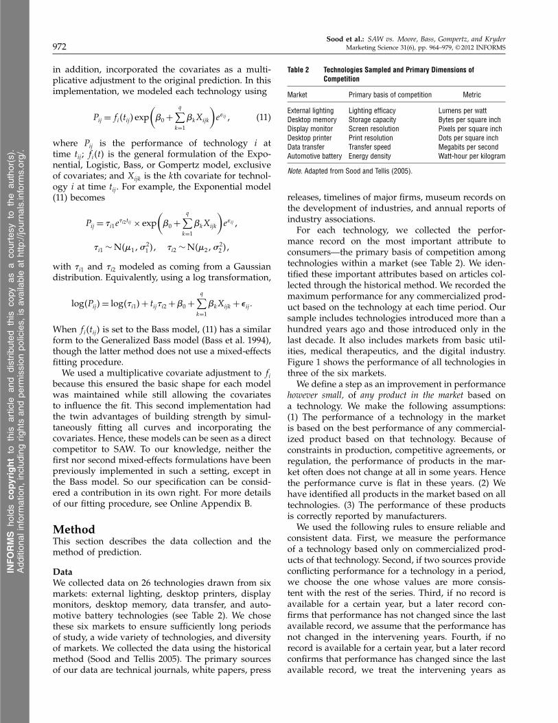
Market Primary basis of competition Metric

External lighting Lighting efficacy Lumens per wattDesktop memory Storage capacity Bytes per square inchDisplay monitor Screen resolution Pixels per square inchDesktop printer Print resolution Dots per square inchData transfer Transfer speed Megabits per secondAutomotive battery Energy density Watt-hour per kilogram

Note. Adapted from Sood and Tellis (2005).

releases, timelines of major firms, museum records onthe development of industries, and annual reports ofindustry associations.

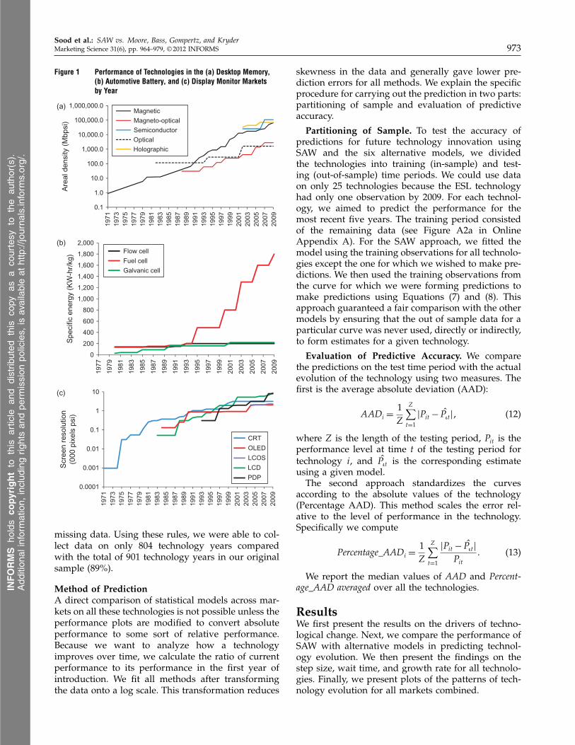
For each technology, we collected the perfor-mance record on the most important attribute toconsumers—the primary basis of competition amongtechnologies within a market (see Table 2). We iden-tified these important attributes based on articles col-lected through the historical method. We recorded themaximum performance for any commercialized prod-uct based on the technology at each time period. Oursample includes technologies introduced more than ahundred years ago and those introduced only in thelast decade. It also includes markets from basic util-ities, medical therapeutics, and the digital industry.Figure 1 shows the performance of all technologies inthree of the six markets.

We define a step as an improvement in performancehowever small, of any product in the market based ona technology. We make the following assumptions:(1) The performance of a technology in the marketis based on the best performance of any commercial-ized product based on that technology. Because ofconstraints in production, competitive agreements, orregulation, the performance of products in the mar-ket often does not change at all in some years. Hencethe performance curve is flat in these years. (2) Wehave identified all products in the market based on alltechnologies. (3) The performance of these productsis correctly reported by manufacturers.

We used the following rules to ensure reliable andconsistent data. First, we measure the performanceof a technology based only on commercialized prod-ucts of that technology. Second, if two sources provideconflicting performance for a technology in a period,we choose the one whose values are more consis-tent with the rest of the series. Third, if no record isavailable for a certain year, but a later record con-firms that performance has not changed since the lastavailable record, we assume that the performance hasnot changed in the intervening years. Fourth, if norecord is available for a certain year, but a later recordconfirms that performance has changed since the lastavailable record, we treat the intervening years as

INFORMS

holds

copyrightto

this

article

and

distrib

uted

this

copy

asa

courtesy

tothe

author(s).

Add

ition

alinform

ation,

includ

ingrig

htsan

dpe

rmission

policies,

isav

ailableat

http://journa

ls.in

form

s.org/.


Figure 1 Performance of Technologies in the (a) Desktop Memory,(b) Automotive Battery, and (c) Display Monitor Marketsby Year

missing data. Using these rules, we were able to col-lect data on only 804 technology years comparedwith the total of 901 technology years in our originalsample (89%).

Method of PredictionA direct comparison of statistical models across mar-kets on all these technologies is not possible unless theperformance plots are modified to convert absoluteperformance to some sort of relative performance.Because we want to analyze how a technologyimproves over time, we calculate the ratio of currentperformance to its performance in the first year ofintroduction. We fit all methods after transformingthe data onto a log scale. This transformation reduces

skewness in the data and generally gave lower pre-diction errors for all methods. We explain the specificprocedure for carrying out the prediction in two parts:partitioning of sample and evaluation of predictiveaccuracy.

Partitioning of Sample. To test the accuracy ofpredictions for future technology innovation usingSAW and the six alternative models, we dividedthe technologies into training (in-sample) and test-ing (out-of-sample) time periods. We could use dataon only 25 technologies because the ESL technologyhad only one observation by 2009. For each technol-ogy, we aimed to predict the performance for themost recent five years. The training period consistedof the remaining data (see Figure A2a in OnlineAppendix A). For the SAW approach, we fitted themodel using the training observations for all technolo-gies except the one for which we wished to make pre-dictions. We then used the training observations fromthe curve for which we were forming predictions tomake predictions using Equations (7) and (8). Thisapproach guaranteed a fair comparison with the othermodels by ensuring that the out of sample data for aparticular curve was never used, directly or indirectly,to form estimates for a given technology.

Evaluation of Predictive Accuracy. We comparethe predictions on the test time period with the actualevolution of the technology using two measures. Thefirst is the average absolute deviation (AAD):

AADi =1Z

Z∑

t=1

�Pit − P̂�t�1 (12)

where Z is the length of the testing period, Pit is theperformance level at time t of the testing period fortechnology i, and P̂�t is the corresponding estimateusing a given model.

The second approach standardizes the curvesaccording to the absolute values of the technology(Percentage AAD). This method scales the error rel-ative to the level of performance in the technology.Specifically we compute

Percentage_AADi =1Z

Z∑

t=1

�Pit − P̂�t�

Pit

0 (13)

We report the median values of AAD and Percent-age_AAD averaged over all the technologies.

ResultsWe first present the results on the drivers of techno-logical change. Next, we compare the performance ofSAW with alternative models in predicting technol-ogy evolution. We then present the findings on thestep size, wait time, and growth rate for all technolo-gies. Finally, we present plots of the patterns of tech-nology evolution for all markets combined.

INFORMS

holds

copyrightto

this

article

and

distrib

uted

this

copy

asa

courtesy

tothe

author(s).

Add

ition

alinform

ation,

includ

ingrig

htsan

dpe

rmission

policies,

isav

ailableat

http://journa

ls.in

form

s.org/.


Table 3 Drivers of Step Size and Wait Time

Step size Wait time

Covariate Est. t-value Est. t-value

Year of introduction (H1) 0019 3907 −0012 −24703Order of entry (H2) −0031 −800 −0005 −103No. of competing technologies (H3) −0011 −300 0042 1204No. of prior steps (H4) −0001 −103 −0006 −604Average prior wait time (H5) 0008 304 −00003 −001

Last step size (r − Equation (3)) 0002 209 00002 003Last wait time (s− Equation (6)) −0004 −208 −0001 −008

Drivers of Technological ChangeTable 3 presents the parameter estimates for the Stepand Wait submodels. The year of introduction covari-ate has a positive sign for the Step submodel but anegative sign for the Wait submodel. The results sup-port H1, that products introduced in later years tendto have shorter waits and larger steps.

The order of entry covariate has negative signsfor both the Step and Wait submodels. The resultsindicate that, after controlling for year of entry, laterentrants to a market tend to have a shorter wait butsmaller steps. The negative coefficient for the step sizeis highly statistically significant and is consistent withthe preferential attraction theory (H2B).

The number of competing technologies covariatehas a negative sign for the Step submodel and a pos-itive sign for the Wait submodel. The results suggestthat after controlling for the effects above, our resultssupport H3A and reject H3B.

The number of prior steps covariate has a nega-tive sign for both the Step and Wait submodels. Theresults support H4 and suggest that technologies thathave a number of prior steps continue to have smallsteps that happen at frequent intervals.

The average prior wait time covariate has a positivesign for the Step submodel but a slightly negative signfor the Wait submodel. The results partially supportH5, suggesting that, after conditioning on the othercovariates, technologies with long average prior waittimes also have larger step sizes but may not continueto have long wait times.

Finally, the last step size and the last wait timecovariates are statistically significant in the Step sub-model, providing evidence that there is a correlationbetween step sizes and wait times, even after adjust-ing for the other covariates.

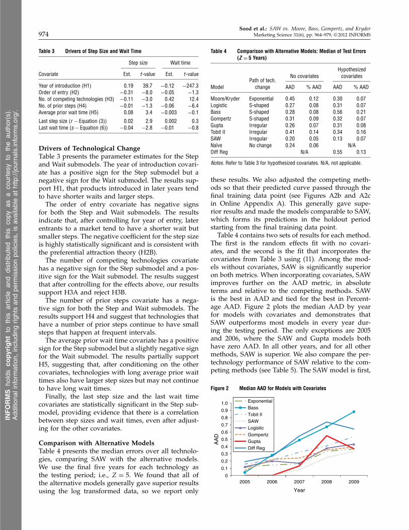
Comparison with Alternative ModelsTable 4 presents the median errors over all technolo-gies, comparing SAW with the alternative models.We use the final five years for each technology asthe testing period; i.e., Z = 5. We found that all ofthe alternative models generally gave superior resultsusing the log transformed data, so we report only

Table 4 Comparison with Alternative Models: Median of Test Errors(Z = 5 Years)

HypothesizedNo covariates covariates

Path of tech.Model change AAD % AAD AAD % AAD

Moore/Kryder Exponential 0045 0012 0030 0007Logistic S-shaped 0027 0008 0031 0007Bass S-shaped 0028 0008 0056 0021Gompertz S-shaped 0031 0009 0032 0007Gupta Irregular 0026 0007 0031 0008Tobit II Irregular 0041 0014 0034 0016SAW Irregular 0020 0005 0013 0007Naïve No change 0024 0006 N/ADiff Reg N/A 0055 0013

Notes. Refer to Table 3 for hypothesized covariates. N/A, not applicable.

these results. We also adjusted the competing meth-ods so that their predicted curve passed through thefinal training data point (see Figures A2b and A2cin Online Appendix A). This generally gave supe-rior results and made the models comparable to SAW,which forms its predictions in the holdout periodstarting from the final training data point.

Table 4 contains two sets of results for each method.The first is the random effects fit with no covari-ates, and the second is the fit that incorporates thecovariates from Table 3 using (11). Among the mod-els without covariates, SAW is significantly superioron both metrics. When incorporating covariates, SAWimproves further on the AAD metric, in absoluteterms and relative to the competing methods. SAWis the best in AAD and tied for the best in Percent-age AAD. Figure 2 plots the median AAD by yearfor models with covariates and demonstrates thatSAW outperforms most models in every year dur-ing the testing period. The only exceptions are 2005and 2006, where the SAW and Gupta models bothhave zero AAD. In all other years, and for all othermethods, SAW is superior. We also compare the per-technology performance of SAW relative to the com-peting methods (see Table 5). The SAW model is first,

Figure 2 Median AAD for Models with Covariates

0

0.1

0.2

0.3

0.4

0.5

0.6

0.7

0.8

0.9

1.0

2005 2006 2007 2008 2009

AA

D

Year

Exponential

Logistic

Bass

Gompertz

Tobit II

Gupta

SAW

Diff Reg

INFORMS

holds

copyrightto

this

article

and

distrib

uted

this

copy

asa

courtesy

tothe

author(s).

Add

ition

alinform

ation,

includ

ingrig

htsan

dpe

rmission

policies,

isav

ailableat

http://journa

ls.in

form

s.org/.


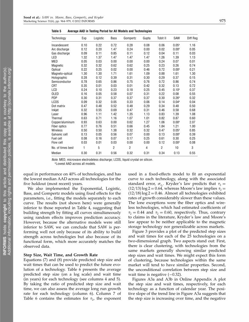
Table 5 Average AAD in Testing Period for All Models and Technologies

Technology Exp Logistic Bass Gompertz Gupta Tobit II SAW Diff Reg

Incandescent 0010 0022 0072 0028 0008 0006 0005a 1016Arc discharge 0012 0020 1047 0024 0000 0002 0000a 0005Gas discharge 0009 0011 0085 0011 0012 0004 0011 0003LED 1032 1037 1047 1047 1047 1026 1039 1013MED 0005 0003 0000 0000 0000 0024 0007 0001Magnetic 0032 0032 0062 0062 0025 0023 0026 0074Optical 0022 0025 0002 0000 0046 0072 0000a 0021Magneto-optical 1030 1030 1071 1061 1009 0088 1061 1030Holographic 0028 0012 0039 0031 0030 0029 0037 0015Semiconductor 0078 0065 0086 0075 0076 0072 0086 0074CRT 0035 0001 0003 0001 0042 0032 0013 0072LCD 0024 0010 0023 0018 0025 0045 0010a 0037OLED 0016 0005 0058 0007 0031 0022 0008 0055PDP 0030 0031 0037 0037 0037 0030 0026a 0032LCOS 0009 0032 0005 0033 0006 0014 0004a 0004Dot matrix 0047 0048 0052 0048 0029 0034 0048 0050Inkjet 0032 0055 0069 0047 0031 0046 0058 0068Laser 0096 1011 1042 1035 1013 0083 1039 1008Thermal 0063 0071 1016 1007 1001 0082 0087 0060Copper/aluminum 0093 0063 0000 0062 1027 1006 0000a 2007Fiber optics 0077 0076 0051 0066 0045 1084 1021 1000Wireless 0050 0050 1038 0032 0032 0047 0005a 0085Galvanic cell 0013 0005 0056 0007 0000 0013 0000a 0039Fuel cell 0008 0016 0007 0017 0025 0061 0030 0025Flow cell 0003 0001 0003 0000 0000 0012 0000a 0008

No. of times best 1 5 2 2 4 2 10 3

Median 0.30 0.31 0.56 0.32 0.31 0.34 0.13 0.55

Note. MED, microwave electrodeless discharge; LCOS, liquid crystal on silicon.aLowest AAD across all models.

equal in performance on 40% of technologies, and hasthe lowest median AAD across all technologies for thefive holdout (most recent) years.

We also implemented the Exponential, Logistic,Bass, and Gompertz models using fixed effects for theparameters, i.e., fitting the models separately to eachcurve. The results (not shown here) were generallyinferior to those reported in Table 4, suggesting thatbuilding strength by fitting all curves simultaneouslyusing random effects improves prediction accuracy.However, because the alternative models were stillinferior to SAW, we can conclude that SAW is per-forming well not only because of its ability to buildstrength across technologies but also because of itsfunctional form, which more accurately matches theobserved data.

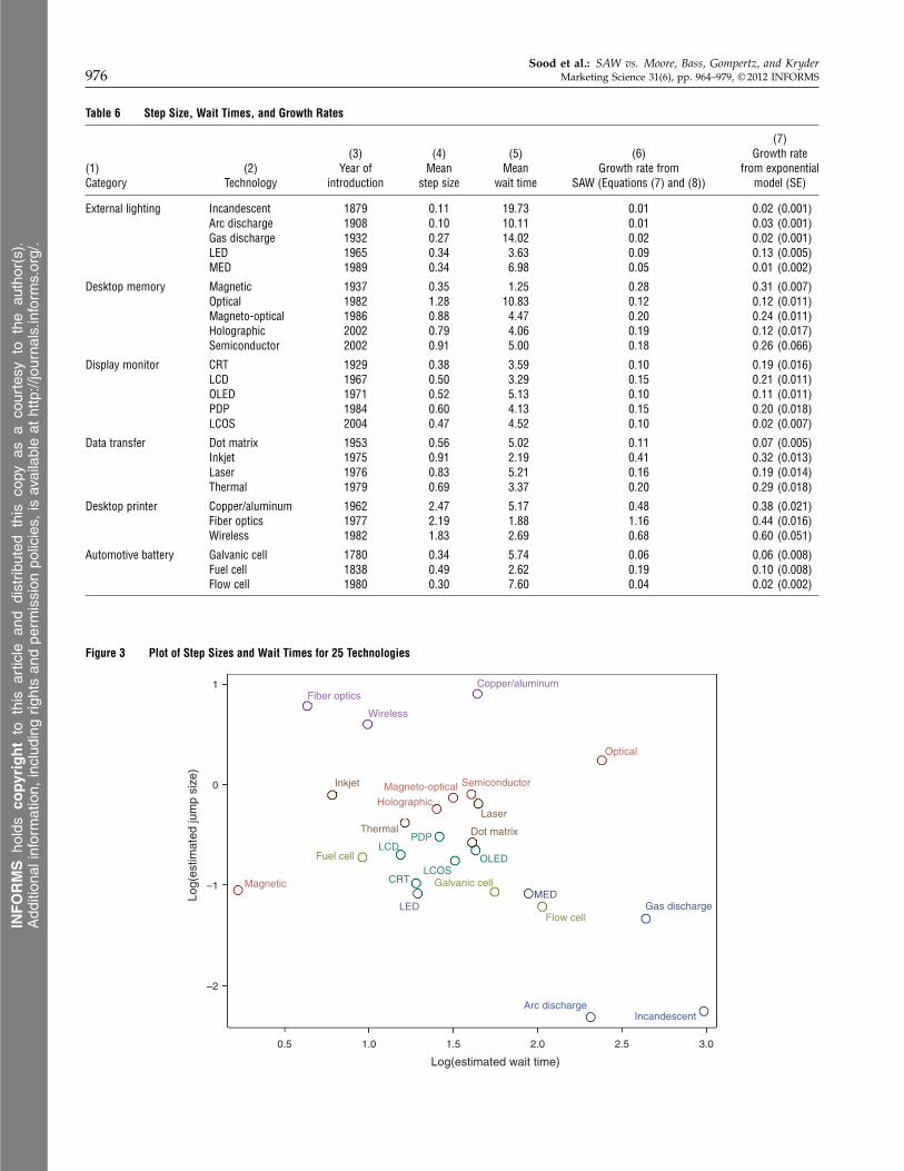
Step Size, Wait Time, and Growth RateEquations (7) and (8) provide predicted step size andwait times that can be used to predict the future evo-lution of a technology. Table 6 presents the averagepredicted step size (on a log scale) and wait time(in years) for each technology (see columns 4 and 5).By taking the ratio of predicted step size and waittime, we can also assess the average long run growthrate for each technology (column 6). Column 7 ofTable 6 contains the estimates for �2, the exponent

used in a fixed-effects model to fit an exponentialcurve to each technology, along with the associatedstandard error, ��2

. Kryder’s law predicts that �2 =

412/135 log 2 = 0064, whereas Moore’s law implies �2 =

412/185 log 2 = 0046. Almost all technologies exhibitedrates of growth considerably slower than these values.The lone exceptions were the fiber optics and wire-less technologies, which had estimated coefficients of�2 = 0044 and �2 = 0060, respectively. Thus, contraryto claims in the literature, Kryder’s law and Moore’slaw appear to be neither applicable to the magneticstorage technology nor generalizable across markets.

Figure 3 provides a plot of the predicted step sizesand wait times for each of the 25 technologies on atwo-dimensional graph. Two aspects stand out: First,there is clear clustering, with technologies from thesame markets generally showing similar predictedstep sizes and wait times. We might expect this formof clustering, because technologies within the samemarket will tend to have similar properties. Second,the unconditional correlation between step size andwait time is negative (−0.32).

Figures A3a and A3b in Online Appendix A plotthe step size and wait times, respectively, for eachtechnology as a function of calendar year. The posi-tive slope of the trend line in Figure A3a suggests thatthe step size is increasing over time, and the negative

INFORMS

holds

copyrightto

this

article

and

distrib

uted

this

copy

asa

courtesy

tothe

author(s).

Add

ition

alinform

ation,

includ

ingrig

htsan

dpe

rmission

policies,

isav

ailableat

http://journa

ls.in

form

s.org/.


Table 6 Step Size, Wait Times, and Growth Rates

(7)(3) (4) (5) (6) Growth rate

(1) (2) Year of Mean Mean Growth rate from from exponentialCategory Technology introduction step size wait time SAW (Equations (7) and (8)) model (SE)

External lighting Incandescent 1879 0011 19073 0001 0002 (0.001)Arc discharge 1908 0010 10011 0001 0003 (0.001)Gas discharge 1932 0027 14002 0002 0002 (0.001)LED 1965 0034 3063 0009 0013 (0.005)MED 1989 0034 6098 0005 0001 (0.002)

Desktop memory Magnetic 1937 0035 1025 0028 0031 (0.007)Optical 1982 1028 10083 0012 0012 (0.011)Magneto-optical 1986 0088 4047 0020 0024 (0.011)Holographic 2002 0079 4006 0019 0012 (0.017)Semiconductor 2002 0091 5000 0018 0026 (0.066)

Display monitor CRT 1929 0038 3059 0010 0019 (0.016)LCD 1967 0050 3029 0015 0021 (0.011)OLED 1971 0052 5013 0010 0011 (0.011)PDP 1984 0060 4013 0015 0020 (0.018)LCOS 2004 0047 4052 0010 0002 (0.007)

Data transfer Dot matrix 1953 0056 5002 0011 0007 (0.005)Inkjet 1975 0091 2019 0041 0032 (0.013)Laser 1976 0083 5021 0016 0019 (0.014)Thermal 1979 0069 3037 0020 0029 (0.018)

Desktop printer Copper/aluminum 1962 2047 5017 0048 0038 (0.021)Fiber optics 1977 2019 1088 1016 0044 (0.016)Wireless 1982 1083 2069 0068 0060 (0.051)

Automotive battery Galvanic cell 1780 0034 5074 0006 0006 (0.008)Fuel cell 1838 0049 2062 0019 0010 (0.008)Flow cell 1980 0030 7060 0004 0002 (0.002)

Figure 3 Plot of Step Sizes and Wait Times for 25 Technologies

Fiber optics

Wireless

Copper/aluminum

Optical

Inkjet SemiconductorMagneto-optical

Laser

ThermalPDP Dot matrix

OLEDFuel cellLCD

LCOSCRT

LED

Magnetic Galvanic cellMED

Flow cellGas discharge

Arc dischargeIncandescent

0.5 1.0 1.5 2.0 2.5 3.0

Log(estimated wait time)

1

0

–1

–2

Log(

estim

ated

jum

p si

ze)

Holographic

INFORMS

holds

copyrightto

this

article

and

distrib

uted

this

copy

asa

courtesy

tothe

author(s).

Add

ition

alinform

ation,

includ

ingrig

htsan

dpe

rmission

policies,

isav

ailableat

http://journa

ls.in

form

s.org/.


slope in Figure A3b suggests that the wait time isdecreasing over time. Figure A3c plots the growth rate(on a log scale) over calendar time and shows a veryclear trend of exponentially increasing growth ratesover calendar time, with a correlation of over 0.6 witha p-value below 1%. These results suggest that tech-nology evolution is occurring at a faster pace withcalendar time.

DiscussionThis section summarizes the findings and discussesthe implications and limitations.

Summary of FindingsThe current research leads to four major findings:

1. The traditional laws of technology evolutionsuch as Moore’s law and Kryder’s law do not gener-alize across markets; none holds for all technologieseven in a single market.

2. SAW produces superior predictions over tradi-tional methods, such as the Bass model or Gompertz’slaw, and can form predictions for a completely newtechnology by incorporating information from othercategories on time-varying covariates.

3. The signs of the significant drivers of technologyevolution suggest that

a. recent technologies improve at a faster ratethan old technologies;

b. as the number of competitors increases, theperformance of technologies increases in smaller stepsand longer waits;

c. later entrants to a market and technologies thathave a number of prior steps tend to have smallersteps and shorter waits; and

d. technologies with long average prior waittimes continue to have large step sizes.

4. Technologies cluster in their performance bymarket.

ImplicationsThis study has several implications for managers.First, our results suggest that popular laws and mod-els such as Moore’s law, Kryder’s law, Gompertz’slaw, and the logistic model are naïve generaliza-tions of what seems to be a complex phenomenon.Such theories make simplistic assumptions aboutthe path of technology evolution (e.g., exponentialor S-shaped) and thus are inadequate in predictingtechnology change well. Surprisingly, over the periodcovered in our analysis, it took 28 months for mag-netic storage technology to double in performance,which is much longer than the commonly espousedversions of Moore’s law claiming that performancedoubles every 18 months (recent) or 12 months (orig-inal). Hence, although such laws may serve as long-term guideposts for industry evolution, using them to

predict the performance of a technology is quite riskyand potentially misleading. On the other hand, SAWexplicitly models the discontinuous nature of the tech-nology evolution curves observed empirically.

Second, SAW can help managers to reduce thenature and extent of uncertainty regarding the futurepath of technology evolution. SAW can be easily fitby a simple maximum likelihood approach and incor-porates time-varying covariates for each technology.Thus, managers can use it to assess the nature of thethreat posed by a competing technology by classifyingit as one that is a long-wait/small-step technology, orvice versa. As an example, consider the competitionbetween LCD and CRT monitors (see Figure 1c). Sonykept investing in CRT technology even after LCDfirst crossed CRT in performance in 1996. Instead ofconsidering LCD, Sony introduced the FD Trinitron/WEGA series, a flat-screen version of the CRT. CRTcrossed LCD for a few years, but ultimately lost deci-sively to LCD in 2001. In contrast, by backing LCDtechnology, Samsung grew to be the world’s largestmanufacturer of LCD monitors, whereas the formerleader Sony had to seek a joint venture with Samsungin 2006 to manufacture LCD monitors. Prediction ofthe next step size and wait time using SAW couldhave helped Sony’s managers make a timely invest-ment in LCD technology.

Third, SAW overcomes limitations of prior modelsof depending on only environmental scanning (e.g.,survey or the Delphi method) or extrapolation (e.g.,trend analysis). SAW incorporates both environmentalscanning by incorporating data from multiple tech-nologies and extrapolation by incorporating past datafrom the target technology in making predictions.Further, SAW is flexible enough to allow for largeperiods of no change punctuated by big steps or smallperiods of small changes, approximating a smoothcurve. As such, it partially resolves the controversyin the literature between technology evolution via asmooth curve (Basalla 1988, Dosi 1982) or via sta-ble periods punctuated with big steps (Eldredge andGould 1972, Tushman and Anderson 1986). For exam-ple, inkjet printers became the dominant technologyin the market even though they had the lowest per-formance at its introduction through a series of smallbut frequent steps.

Fourth, our results suggest that the competitivelandscape is becoming more intense. An increasingnumber of new technologies is entering the mar-ket. The rate of technology evolution is increasing ata faster pace. Thus, managers need a method andmodel to predict technology evolution to guide theirmultimillion dollar investments. SAW serves such apurpose. SAW can easily make predictions for a newtechnology with no prior data. This discussion bringsus back to the key question that managers face: Which

INFORMS

holds

copyrightto

this

article

and

distrib

uted

this

copy

asa

courtesy

tothe

author(s).

Add

ition

alinform

ation,

includ

ingrig

htsan

dpe

rmission

policies,

isav

ailableat

http://journa

ls.in

form

s.org/.


technology to back? In GM’s case, it turned out to bea billion-dollar question. GM spent over a billion dol-lars on the hydrogen fuel cell. Yet the technology thatleapt ahead in the 2000s was lithium-ion. Tesla basedits battery on lithium-ion technology and had a car onthe market in 2006. GM saw the need for lithium-iononly after the Tesla car was launched, and it launcheda car using a lithium-ion battery only in December2010. Many firms were taken by surprise by the sud-den dominance of lithium-ion. Managers might havepresaged the improvements in lithium-ion technologybefore 2006 by using our model.

LimitationsThis study has five limitations. First, we had to limitour analysis to only six markets because of the timeand difficulty of data collection. Second, our anal-ysis does not include the impact of investments inR&D on technology evolution. This is a limitation ofthe data, rather than of SAW, as it could certainlyinclude R&D budgets as a covariate, which shouldincrease its predictive accuracy even more. Third, ouranalysis does not include the cost of the technologyto buyers. Fourth, it is not possible to exactly esti-mate the step size and wait times for the years withmissing data. However, given the small percentage ofsuch data, this is unlikely to have a significant effecton the results. Fifth, we assume that firms announceall improvements in performance and that there areno minor improvements between steps. A possibleextension may relax this assumption and allow for alow level of growth during the wait period. All ofthese limitations are potential opportunities for futureresearch.

Electronic CompanionAn electronic companion to this paper is available aspart of the online version at http://dx.doi.org/10.1287/mksc.1120.0739.

AcknowledgmentsThe study benefited from Dean’s Research Grant Award,Emory University, a gift of Don Murray to the Univer-sity of Southern California Marshall Center for GlobalInnovation, and from the comments of participants atthe Institute for the Study of Business Markets AcademicConference, American Marketing Association Winter Con-ference, Marketing Science conference, and BPS/TIM/ENTPanel Symposium at the Annual Meeting of the Academyof Management.

ReferencesAbernathy WJ, Utterback JM (1978) Patterns of industrial innova-

tion. Tech. Rev. 80(7):40–47.Adner R (2002) When are technologies disruptive: A demand-based

view of the emergence of competition. Strategic Management J.23(8):667–688.

Armstrong JS (1984) Forecasting by extrapolation: Conclusionsfrom 25 years of research. Interfaces 14(6):52–66.

Arrow KJ (1962) Economic welfare and the allocation of resourcesfor invention. Nelson RR, ed. The Rate and Direction of EconomicActivity (Princeton University Press, Princeton, NJ), 609–625.

Balachandra R (1980) Technological forecasting: Who does it andhow useful is it? Tech. Forecasting Soc. Change 16(1):75–85.

Basalla G (1988) The Evolution of Technology (Cambridge UniversityPress, Cambridge, UK).

Bass FM (1969) A new product growth for model consumerdurables. Management Sci. 15(5):215–227.

Bass FM, Krishnan TV, Jain DC (1994) Why the Bass model fitswithout decision variables. Marketing Sci. 13(3):203–223.

Brown R (1992) Managing “S” curves of innovation. J. ConsumerMarketing 9(1):61–73.

Chandy RK, Tellis GJ (2000) The incumbent’s curse? Incumbency,size, and radical product innovation. J. Marketing 64(3):1–17.

Cox D (1970) Renewal Theory (Methuen & Co., London).D’Aveni RA (1994) Hypercompetition: Managing the Dynamics of

Strategic Maneuvering (Free Press, New York).Dosi G (1982) Technological paradigms and technological trajecto-

ries. Res. Policy 11(3):147–162.Edwards C (2008) The many lives of Moore’s law. Engrg. Tech.

3(1):36–39.Eldredge N, Gould SJ (1972) Punctuated equilibria: An alternative

to phyletic gradualism. Schopf TJM, ed. Models in Paleobiology(Freeman, Cooper and Co.), 82–115.

Fellner W (1961) Two propositions in the theory of induced inno-vations. Econom. J. 71(282):305–308.

Fleming L (2001) Recombinant uncertainty in technological search.Management Sci. 47(1):117–132.

Foster RD (1986) Innovation: The Attacker’s Advantage (SummitBooks, New York).

Gersick CJG (1991) Revolutionary change theories: A multilevelexploration of the punctuated equilibrium paradigm. Acad.Management Rev. 16(1):10–36.

Golder PN, Tellis GJ (1993) Pioneering advantage: Marketing logicor marketing legend. J. Marketing Res. 30(2):158–170.

Golder PN, Tellis GJ (2004) Growing, growing, gone: Cascades, dif-fusion, and turning points in the product life cycle. MarketingSci. 23(2):207–218.

Gompertz B (1825) On the nature of the function expressive of thelaw of human mortality, and on a new mode of determiningthe value of life contingencies. Philos. Trans. Royal Soc. London115:513–585.

Grochowski E (1998) Emerging trends in data storage on magnetichard disk drives. Datatech (September):11–17.

Gupta S (1988) Impact of sales promotions on when, what, andhow much to buy. J. Marketing Res. 25(4):342–355.

Hauser J, Tellis GJ, Griffin A (2007) Research on innovation:A review and agenda for Marketing Science. Marketing Sci.25(6):687–717.

Henderson RM, Clark KB (1990) Architectural innovation: Thereconfiguration of existing product technologies and the failureof established firms. Admin. Sci. Quart. 35(1):9–30.

Lambkin M (1988) Order of entry and performance in new markets.Strategic Management J. 9(S1):127–140.

Levinthal DA (1998) The slow pace of rapid technological change:Gradualism and punctuation in technological change. Indust.Corporate Change 7(2):217–247.

Makridakis S, Anderson A, Carbone R, Fildes R, Hibon M,Lewandowski R, Newton J, Parzen P, Winkler R (1982) Theaccuracy of extrapolation (time series) methods: Results of aforecasting competition. J. Forecasting 1(2):111–153.

INFORMS

holds

copyrightto

this

article

and

distrib

uted

this

copy

asa

courtesy

tothe

author(s).

Add

ition

alinform

ation,

includ

ingrig

htsan

dpe

rmission

policies,

isav

ailableat

http://journa

ls.in

form

s.org/.


Martino JP (2003) A review of selected advances in technologicalforecasting. Tech. Forecasting Soc. Change 70(8):719–733.

Meade N, Islam T (1995) Forecasting with growth curves:An empirical comparison. Internat. J. Forecasting 11(2):199–215.

Meade N, Islam T (1998) Technological forecasting—Model selec-tion, model stability, and combining models. Management Sci.44(8):1115–1130.

Meade N, Islam T (2006) Modeling and forecasting the diffu-sion of innovation—A 25 year review. Internat. J. Forecasting22(3):519–545.

Mollick E (2006) Establishing Moore’s law. IEEE Ann. History Com-put. 28(3):62–75.

Moore GE (1965) Cramming more components onto integratedcircuits. Electronics 38(8):114–117. http://www.intel.com/research/silicon/moorespaper.pdf.

Moore GE (1975) Progress in digital integrated electronics. IEEE,IEDM Tech Digest 21:11–3.

Moore GE (1995) Lithography and the future of Moore’s law.Warlaumont JM, ed. Electron-Beam, X-Ray, and Ion-Beam Submi-crometer Lithographies for Manufacturing V: Proc. SPIE, Vol. 2437(SPIE, Bellingham, WA), 1–4.

Moore GE (1997) An update on Moore’s law. Intel Developer ForumKeynote, September 30, Intel, Santa Clara, CA.

Moore GE (2003) No exponential is forever: But “forever” can bedelayed! Solid-State Circuits Conf. 2003, Digest Tech. Papers, IEEEInternat., Vol. 1 (IEEE, New York), 20–23.

Nelson RR, Winter SG (1977) In search of useful theory of innova-tion. Res. Policy 6(1):36–76.

Nelson RR, Winter SG (1982) An Evolutionary Theory of Eco-nomic Change (Belknap Press/Harvard University Press,Cambridge, MA).

Pinheiro JC, Bates DM (2000) Mixed-Effects Models in S and S PLUS(Statistics and Computing Series) (Springer-Verlag, New York).

Rogers EM (1962) Diffusion of Innovations (Free Press, New York).Rosenberg N (1969) The direction of technological change: Induce-

ment mechanisms and focusing devices. Econom. DevelopmentCultural Change 18(1):1–24.

Sahal D (1981) Alternative conceptions of technology. Res. Policy10(1):2–24.

Schaller RR (1997) Moore’s law: Past, present and future. SpectrumIEEE 34(6):52–59.

Scherer FM (1967) Market structure and the employment of scien-tists and engineers. Amer. Econom. Rev. 57(June):524–531.

Scherer FM, Ross D (1990) Industrial Market Structure and EconomicPerformance (Houghton Mifflin, New York).

Shacklett M (2008) Storage density and Kryder’s law. Byte SwitchNews Anal. 11:19.

Sood A, Tellis GJ (2005) Technological evolution and radical inno-vations. J. Marketing 69(3):152–168.

Sood A, Tellis GJ (2011) Demystifying disruption: A new model forunderstanding and predicting disruptive technologies. Market-ing Sci. 30(2):339–354.

Sood A, James GM, Tellis GJ (2009) Functional regression: A newmodel for predicting market penetration of new products. Mar-keting Sci. 28(1):36–51.

Tashman LJ (2000) Out-of-sample tests of forecasting accuracy:An analysis and review. Internat. J. Forecasting 16(4):437–450.

Tellis GJ (2008) Important research questions in technology andinnovation. Indust. Marketing Management 37(6):629–632.

Tushman ML, Anderson P (1986) Technological discontinuities andorganizational environments. Admin. Sci. Quart. 31(3):439–465.

Tushman ML, Romanelli E (1985) Organizational evolution:A metamorphosis model of convergence and reorientation. Res.Organ. Behav. 7:171–222.

Urban GL, Carter T, Gaskin S, Mucha Z (1986) Market sharerewards to pioneering brands: An empirical analysis andstrategic implications. Management Sci. 32(6):645–659.

Utterback JM, Abernathy WJ (1975) A dynamic model of processand product innovation. Omega 3(6):639–656.

Walter C (2005) Kryder’s law. Scientific Amer. 293(2):32–33.Wolff MF (2004) Chase Moore’s law, inventors urged. Res. Tech.

Management 47(1):6.Wollin A (1999) Punctuated equilibrium: Reconciling theory of rev-

olutionary and incremental change. Systems Res. Behav. Sci.16(4):359–367.

Young P (1993) Technological growth curves: A competition of fore-casting models. Tech. Forecasting Soc. Change 44(4):375–389.

Young P, Ord JK (1989) Model selection and estimation for techno-logical growth curves. Internat. J. Forecasting 5(5):501–513.

INFORMS

holds

copyrightto

this

article

and

distrib

uted

this

copy

asa

courtesy

tothe

author(s).

Add

ition

alinform

ation,

includ

ingrig

htsan

dpe

rmission

policies,

isav

ailableat

http://journa

ls.in

form

s.org/.

Documents

Predicting the Path of Technological Innovation: SAW vs ...gareth/research/MktSciSAW.pdf · Predicting the Path of Technological Innovation: SAW vs. Moore, Bass, Gompertz, and Kryder