1

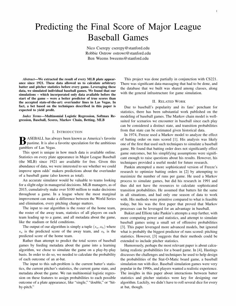
Predicting the Final Score of Major LeagueBaseball Games

Nico Cserepy cserepy@stanford.eduRobbie Ostrow ostrowr@stanford.edu

Ben Weems bweems@stanford.edu

Abstract—We extracted the result of every MLB plate appear-ance since 1921. These data allowed us to calculate arbitrarybatter and pitcher statistics before every game. Leveraging thesedata, we simulated individual baseball games. We found that oursimulations – which incorporated only data available before thestart of the game – were a better predictor of true scores thanthe accepted state-of-the-art: over/under lines in Las Vegas. Infact, a bet based on the techniques described in this paper isexpected to yield profit.

Index Terms—Multinomial Logistic Regression, Softmax Re-gression, Baseball, Scores, Markov Chain, Betting, MLB

I. INTRODUCTION

BASEBALL has always been known as America’s favoritepastime. It is also a favorite speculation for the ambitious

gamblers of Las Vegas.This sport is unique in how much data is available online.

Statistics on every plate appearance in Major League Baseball(the MLB) since 1921 are available for free. Given thisabundance of data, we were interested to see whether we couldimprove upon odds’ makers predictions about the over/underof a baseball game (also known as total).

An accurate simulator would be valuable to teams lookingfor a slight edge in managerial decisions. MLB managers, as of2015, cumulatively make over $100 million to make decisionsthroughout a game. In a league where the most marginalimprovement can make a difference between the World Seriesand elimination, every pitching change matters.

The input to our algorithm is the roster of the home team,the roster of the away team, statistics of all players on eachteam leading up to a game, and all metadata about the game,like the stadium or field conditions.

The output of our algorithm is simply a tuple (sa

, ah

) wheresa

is the predicted score of the away team, and sh

is thepredicted score of the home team.

Rather than attempt to predict the total scores of baseballgames by feeding metadata about the game into a learningalgorithm, we chose to simulate the game on a play-by-playbasis. In order to do so, we needed to calculate the probabilityof each outcome of an at-bat.

The input to this sub-problem is the current batter’s statis-tics, the current pitcher’s statistics, the current game state, andmetadata about the game. We ran multinomial logistic regres-sion on these features to assign probabilities to each possibleoutcome of a plate appearance, like “single,” “double,” or “hit-by-pitch.”

This project was done partially in conjunction with CS221.There was significant data-massaging that had to be done, andthe database that we built was shared among classes, alongwith the general infrastructure for game simulation.

II. RELATED WORK

Due to baseball’s popularity and its fans’ penchant forstatistics, there has been substantial work published on themodeling of baseball games. The Markov chain model is well-suited for scenarios we encounter in baseball since each playcan be considered a distinct state, and transition probabilitiesfrom that state can be estimated given historical data.

In 1974, Freeze used a Markov model to analyze the effectof batting order on runs scored [1]. His analysis was likelyone of the first that used such techniques to simulate a baseballgame. He found that batting order does not significantly effectgame outcomes, but his simplifying assumptions were signifi-cant enough to raise questions about his results. However, histechniques provided a useful model for future research.

Pankin attempted a more sophisticated version of Freeze’sresearch to optimize batting orders in [2] by attempting tomaximize the number of runs per game. He used a Markovprocess to simulate games, but did his research in 1991 andthus did not have the resources to calculate sophisticatedtransition probabilities. He assumed that batters hit the samein all situations, and had only one season of data to workwith. His methods were primitive compared to what is feasibletoday, but his was the first paper that proved that Markovprocesses can be leveraged for an advantage in baseball.

Bukiet and Elliote take Pankin’s attempts a step further, withmore computing power and statistics, and attempt to simulatebaseball games using a small set of offensive probabilities[3]. This paper leveraged more advanced models, but ignoredwhat is probably the biggest predictor of runs scored: pitchingstatistics. However, [3] suggests that their methods could beextended to include pitcher statistics.

Humorously, perhaps the most relevant paper is about calcu-lating realistic probabilities for a board game. In [4], Hastingsdiscusses the challenges and techniques he used to help designthe probabilities of the Stat-O-Matic board game, a baseballsimulation run with dice. Baseball simulation games were verypopular in the 1990s, and players wanted a realistic experience.The insights in this paper about interactions between batterstatistics and pitcher statistics were key for designing ouralgorithm. Luckily, we didn’t have to roll several dice for everyat bat, though.

2

III. DATASET AND FEATURES

To convey our need for a large volume of data, we haveincluded our feature templates:

Binary feature templates. Each of these features assumesa value in {0, 1}. Brackets signify where more thanone possible feature exists. For example, there is a separatebinary feature for man_on_base_2 and man_on_base_3.

{0, 1, 2} out {1, 2, ...} inningman on base {1, 2, 3} {0, 1, 2...} stadium{0, 1, 2...} precipitation {0, 1, 2...} wind direction{0, 1, 2...} field condition batter and pitcher same handed

Real-valued feature templates. Each of these featurestakes on a real value in [0, 1]. {e} 2 {GenericOut, Strikeout, Advancing Out, Walk,Intentional Walk, Hit by Pitch, Error,Fielder’s Choice, Single, Double, Triple,Home Run}.bat signifies a batter’s statistic, pit signifies a pitcher’s

statistic, and limit signifies that only the last 30 events forthat player in that category were considered. For example,single_bat_vs_diff_handed is the number of singlesper plate appearance against a different handed pitcher in thisbatter’s career, and double_pit_totals_limit is thefraction of doubles given up by the pitcher in the last 30 atbats.

{e} bat vs same handed {e} bat vs same handed limit{e} bat vs diff handed {e} bat vs diff handed limit{e} bat totals {e} bat totals limit{e} pit vs same handed {e} pit vs same handed limit{e} pit vs diff handed {e} pit vs diff handed limit{e} pit totals {e} pit totals limit

In total, these feature templates generate 365 features.We believe that these features provide a state-of-the-artdescription of an arbitrary plate-appearance, and they providedeeper knowledge than any model found in the literature.

To calculate these features, we extracted play-by-play datafrom retrosheet.org for all regular-season baseball games sincethe 1921 season [5]. We focused on the data most relevantto modern day by gathering statistics for players who wereactive in the 1980-2014 range. However, players whose careersstarted before 1980 have their career statistics stored.

There were about 7.2 million plate appearances between1980 and 2014. We needed many statistics about each batterand each pitcher specific to the day of each game, but gatheringthese data in real-time would be infeasible. Gathering the dataduring each the simulation would be too slow, so we had toprecompute all of these statistics. In order to perform accuratesimulations, every player needed up-to-date statistics for everygame. We pre-processed the play by play data to calculateall relevant statistics for every player in the starting lineupsof every game between 1980 and 2014. This database endedup being about 50 gigabytes, but proper indexing provideda significant speedup relative to recalculating features everysimulation.

Along with batter and pitcher statistics leading up to thegame, we also had features that depended on the game state.Statistics such as the number of outs, the inning, or the handed-ness of the pitcher might affect the outcome of some plateappearance. Since these features could, by definition, not be

precomputed, we added them to the feature set during eachsimulation.

Unfortunately, an example of the play-by-play data is toolarge to be displayed here. However, we used Chadwick [6] tohelp parse the data from retrosheet.org, and the approximateschema of the original play-by-play data can be found at [6]1.

To train our classifier, we randomly sampled one millionevents along with their results2 from the 7.2 million at-batsavailable after 1980. We also sampled 300,000 at-bats as a“test set.” In our case, since there is no ground truth, analyzingsuccess on a test set is tricky. Rather than a percentage“correct,” we calculate the log-likelihood of our whole testset given the trained classifier. This log-likelihood can becompared to log-likelihoods of other classifiers to determinewhich is superior.

IV. METHODS

Baseball games are sufficiently random and complex that itis not reasonable to model a game as a single vector of featuresand expect that any machine-learning algorithm will be ableto give accurate predictions. Instead, we model the game ona state-by-state basis by running Monte Carlo simulations ona Markov Decision Process (MDP).

To do so, we discretize each baseball game into states thatrepresent plate appearances. This requires that we assume thatnothing happens between the end of two plate appearances.As such, our simulation assumes no steals, passed balls, pick-offs, or other events that might happen during an at-bat. Whilethis may seem like a large assumption to make, these playsturn out to have very little bearing on the score of the gamesince they happen comparatively infrequently [7].

Baseball is a unique sport in the sense that the beginningof each play can be considered a distinct state, and relevantinformation about this state can be easily described. In ourprogram, we define each state to contain the following infor-mation: score of each team, which bases are occupied, thestatistics of the baserunner on each base, the current battingteam, the number of outs, the current inning number, statisticsof the player at bat, statistics of the pitcher, and auxiliary infor-mation. “Auxiliary information” is miscellaneous informationthat does not change from state to state, like the ballpark, hometeam, etc.

Let action be any way a batter can end his at-bat.From each state, there are up to 12 possible actions:{Generic Out, Strikeout, Advancing Out,Walk, Intentional Walk, Hit by Pitch,Error, Fielder’s Choice, Single, Double,Triple and Home Run}. Some actions are not possiblefrom some states. For example, “Fielder’s Choice” is notpossible if there are no runners on base. From each state,we can calculate the probability of each possible action:P (action|state). This calculation of P (action|state) isfundamentally the most difficult and important part of thealgorithm.

1See http://chadwick.sourceforge.net/doc/cwtools.html2Computer ran out of RAM using more than this, but we could feasibly

train on more events.

3

Once we have calculated the probability of each action, wetake a weighted random sample. Having chosen an action, wecan calculate the probability of each outcome given that actionfrom the historical data and again take a weighted sample. Forthis step, we only take into account the positions of the base-runners and the action chosen. For example,P (first and third, no runs scored, no outs made|first, single) is asking the question, “what’s the probabilitythat, after the play, there are players on first and third, noouts are made, and no runs are scored, given that there was abaserunner on first and the batter hit a single?” (The answeris

64253

231220

, or a little less than 28%.) These probabilities arepre-computed to make the simulation run quickly, so they donot depend on the batter or pitcher. Since there are a largenumber of states and transitions, many of which have to becomputed on the spot, we cannot specify a full MDP. Instead,we run Monte Carlo simulations on the states and transitionsspecified above. So, at a very high level, to simulate a singlegame once, we do the following:

1) Enter start state (Away team hitting, nobody on base,etc.)

2) Repeat until game enda) Calculate P (actions|state)b) Choose weighted random actionc) Calculate P (outcomes|action)d) Choose weighted random outcomee) Go to the state that outcome specifies

3) Gather statistics about simulationIn order to achieve statistical significance, we simulate each

game many times. The key to simulating accurate games islearning P (actions|state).

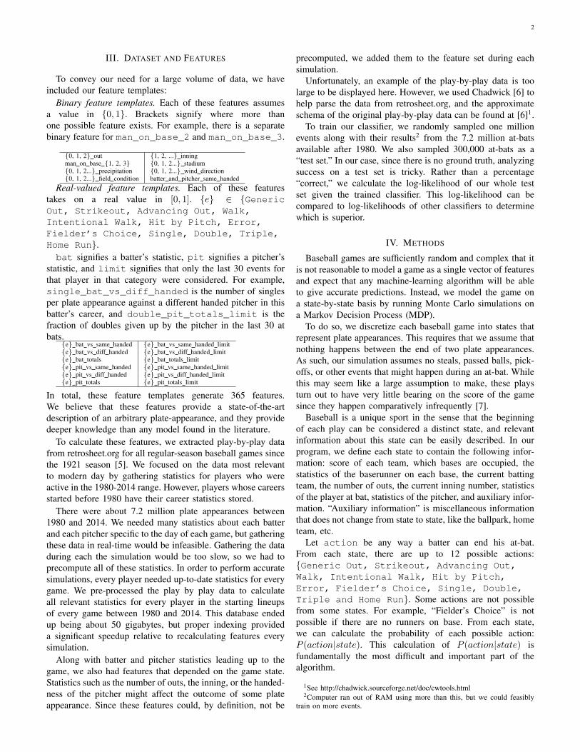
Figure 1: This histogram represents the scores predicted by10,000 simulations of a Mets-Cardinals game. The mediantotal score of the simulations is 8. The actual total score ofthe game was 9.

A. Calculating P(actions|state)

Recall that we have one million training examples each con-sisting of 365 sparse features, all labeled with their outcome.

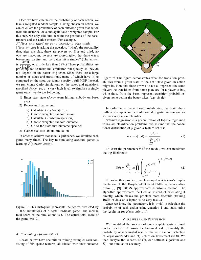
Figure 2: This figure demonstrates what the transition prob-abilities from a given state to the next state given an actionmight be. Note that these arrows do not all represent the sameplayer: the transitions from home plate are for a player at-bat,while those from the bases represent transition probabilitiesgiven some action the batter takes (e.g. single).

In order to estimate these probabilities, we train thesemillion examples on a multinomial logistic regression, orsoftmax regression, classifier.

Softmax regression is a generalization of logistic regressionto n-class classification problems. We assume that the condi-tional distribution of y given a feature set x is

p(y = i|x; ✓) = e✓>i x

kPj=1

e✓>j x

(1)

To learn the parameters ✓ of the model, we can maximizethe log-likelihood:

`(✓) =

mX

i=1

log

kY

l=1

0

BBB@e✓

>k x

(i)

kPj=1

e✓>j x

(i)

1

CCCA

1{y(i)=l}

(2)

To solve this problem, we leveraged scikit-learn’s imple-mentation of the Broyden–Fletcher–Goldfarb–Shanno algo-rithm [8] [9]. BFGS approximates Newton’s method. Thealgorithm approximates the Hessian instead of calculating itdirectly, which makes the problem more tractable (training10GB of data on a laptop is no easy task...)

Once we know the parameters, it is trivial to calculate theprobability of each action using equation 1 and substitutingthe results in for p(action|state).

V. RESULTS AND DISCUSSION

We quantified the success of our complete system basedon two metrics: A) using the binomial test to quantify theprobability of meaningful results relative to random selectionof Vegas over/under and B) Return on Investment (ROI). Wethen analyze the success of C), our softmax algorithm andD), our simulation accuracy.

4

A. Binomial TestPr

edic

tions

Prediction Confusion Matrix

True Result

Over Push Under

Over ci

= 1

di

= 0

ci

= 0

di

= ↵i

ci

= 0

di

= 0

Push No Bet No Bet No Bet

Under ci

= 0

di

= 0

ci

= 0

di

= ↵i

ci

= 1

di

= 0

Table I: Confusion Matrix that determines how to set thevariables c

i

and di

based on a prediction and a result.

To calculate significance relative to random selection, we useda one-tailed binomial test. Our null hypothesis H0 is that theprobability of success (⇡) is 0.5, and our alternative hypothesisH1 is ⇡ > .5. We evaluated our number of successes (k) outof total non-push3 game attempts (n) to measure significance(p). We define c

i

to be 1 if the game was correctly identifiedand 0 if the prediction is incorrect, and set d

i

equal to theamount bet if the result is a push, otherwise it is set to 0.

k = max(

nX

i=0

ci

,

nX

i=0

(1� ci

)) (3)

p = Pr(X � k) =

kX

i=0

✓n

i

◆⇡i

(1� ⇡)n�i (4)

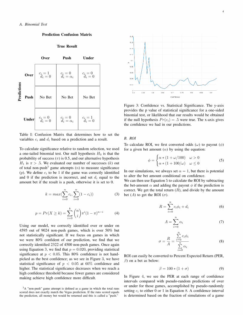
Using our model, we correctly identified over or under on4595 out of 9024 non-push games, which is over 50% butnot statistically significant. If we focus on games in whichwe were 80% confident of our prediction, we find that wecorrectly identified 2322 of 4500 non-push games. Once againusing Equation 3, we find that p = 0.020, providing statisticalsignificance at p < 0.05. This 80% confidence is not hand-picked as the best confidence; as we see in Figure 3, we havestatistical significance of p < 0.05 at 60% confidence andhigher. The statistical significance decreases when we reach ahigh confidence threshold because fewer games are consideredmaking achieve high confidence more difficult.

3A ”non-push” game attempt is defined as a game in which the total runsscored does not exactly match the Vegas prediction. If the runs scored equalsthe prediction, all money bet would be returned and this is called a ”push.”

Figure 3: Confidence vs. Statistical Significance. The y-axisprovides the p value of statistical significance for a one-sidedbinomial test, or likelihood that our results would be obtainedif the null hypothesis Pr(c

i

) = .5 were true. The x-axis givesthe confidence we had in our predictions.

B. ROI

To calculate ROI, we first converted odds (!) to payout (�)for a given bet amount (↵) by using the equation:

� =

(↵ ⇤ (1 + !/100) ! > 0

↵ ⇤ (1 + 100/!) ! 0

(5)

In our simulations, we always set ↵ = 1, but there is potentialto alter the bet amount conditional on confidence.We can then use Equation 5 to calculate the ROI by subtractingthe bet-amount ↵ and adding the payout � if the prediction iscorrect. We get the total return (R), and divide by the amountbet (A) to get the ROI (�).

R =

nX

i=0

ci

�i

+ di

(6)

A =

nX

i=0

↵i

(7)

� =

R

A=

nPi=0

ci

�i

nPi=0

↵i

(8)

ROI can easily be converted to Percent Expected Return (PER,�) on a bet as below:

� = 100 ⇤ (1 + �) (9)

In Figure 4, we see the PER at each range of confidenceintervals compared with pseudo-random predictions of overor under for those games, accomplished by pseudo-randomlysetting c

i

to either 0 or 1 in Equation 8. A confidence intervalis determined based on the fraction of simulations of a game

5

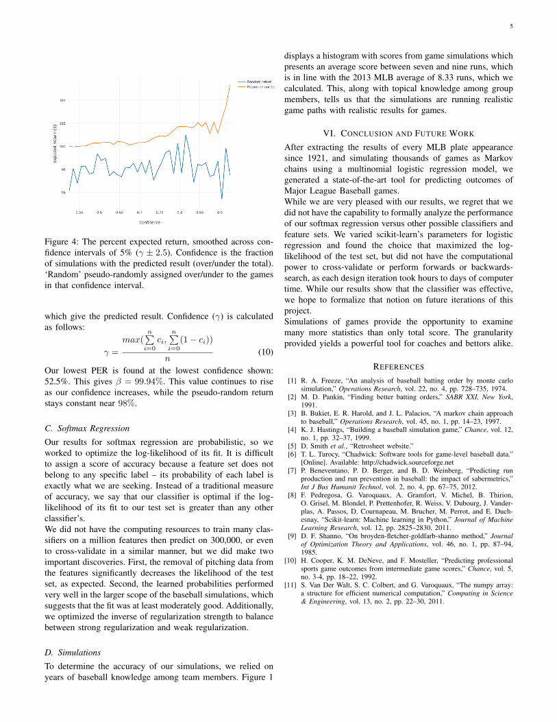
Figure 4: The percent expected return, smoothed across con-fidence intervals of 5% (� ± 2.5). Confidence is the fractionof simulations with the predicted result (over/under the total).‘Random’ pseudo-randomly assigned over/under to the gamesin that confidence interval.

which give the predicted result. Confidence (�) is calculatedas follows:

� =

max(nP

i=0ci

,nP

i=0(1� c

i

))

n(10)

Our lowest PER is found at the lowest confidence shown:52.5%. This gives � = 99.94%. This value continues to riseas our confidence increases, while the pseudo-random returnstays constant near 98%.

C. Softmax RegressionOur results for softmax regression are probabilistic, so weworked to optimize the log-likelihood of its fit. It is difficultto assign a score of accuracy because a feature set does notbelong to any specific label – its probability of each label isexactly what we are seeking. Instead of a traditional measureof accuracy, we say that our classifier is optimal if the log-likelihood of its fit to our test set is greater than any otherclassifier’s.We did not have the computing resources to train many clas-sifiers on a million features then predict on 300,000, or evento cross-validate in a similar manner, but we did make twoimportant discoveries. First, the removal of pitching data fromthe features significantly decreases the likelihood of the testset, as expected. Second, the learned probabilities performedvery well in the larger scope of the baseball simulations, whichsuggests that the fit was at least moderately good. Additionally,we optimized the inverse of regularization strength to balancebetween strong regularization and weak regularization.

D. SimulationsTo determine the accuracy of our simulations, we relied onyears of baseball knowledge among team members. Figure 1

displays a histogram with scores from game simulations whichpresents an average score between seven and nine runs, whichis in line with the 2013 MLB average of 8.33 runs, which wecalculated. This, along with topical knowledge among groupmembers, tells us that the simulations are running realisticgame paths with realistic results for games.

VI. CONCLUSION AND FUTURE WORK

After extracting the results of every MLB plate appearancesince 1921, and simulating thousands of games as Markovchains using a multinomial logistic regression model, wegenerated a state-of-the-art tool for predicting outcomes ofMajor League Baseball games.While we are very pleased with our results, we regret that wedid not have the capability to formally analyze the performanceof our softmax regression versus other possible classifiers andfeature sets. We varied scikit-learn’s parameters for logisticregression and found the choice that maximized the log-likelihood of the test set, but did not have the computationalpower to cross-validate or perform forwards or backwards-search, as each design iteration took hours to days of computertime. While our results show that the classifier was effective,we hope to formalize that notion on future iterations of thisproject.Simulations of games provide the opportunity to examinemany more statistics than only total score. The granularityprovided yields a powerful tool for coaches and bettors alike.

REFERENCES

[1] R. A. Freeze, “An analysis of baseball batting order by monte carlosimulation,” Operations Research, vol. 22, no. 4, pp. 728–735, 1974.

[2] M. D. Pankin, “Finding better batting orders,” SABR XXI, New York,1991.

[3] B. Bukiet, E. R. Harold, and J. L. Palacios, “A markov chain approachto baseball,” Operations Research, vol. 45, no. 1, pp. 14–23, 1997.

[4] K. J. Hastings, “Building a baseball simulation game,” Chance, vol. 12,no. 1, pp. 32–37, 1999.

[5] D. Smith et al., “Retrosheet website.”[6] T. L. Turocy, “Chadwick: Software tools for game-level baseball data.”

[Online]. Available: http://chadwick.sourceforge.net[7] P. Beneventano, P. D. Berger, and B. D. Weinberg, “Predicting run

production and run prevention in baseball: the impact of sabermetrics,”Int J Bus Humanit Technol, vol. 2, no. 4, pp. 67–75, 2012.

[8] F. Pedregosa, G. Varoquaux, A. Gramfort, V. Michel, B. Thirion,O. Grisel, M. Blondel, P. Prettenhofer, R. Weiss, V. Dubourg, J. Vander-plas, A. Passos, D. Cournapeau, M. Brucher, M. Perrot, and E. Duch-esnay, “Scikit-learn: Machine learning in Python,” Journal of MachineLearning Research, vol. 12, pp. 2825–2830, 2011.

[9] D. F. Shanno, “On broyden-fletcher-goldfarb-shanno method,” Journalof Optimization Theory and Applications, vol. 46, no. 1, pp. 87–94,1985.

[10] H. Cooper, K. M. DeNeve, and F. Mosteller, “Predicting professionalsports game outcomes from intermediate game scores,” Chance, vol. 5,no. 3-4, pp. 18–22, 1992.

[11] S. Van Der Walt, S. C. Colbert, and G. Varoquaux, “The numpy array:a structure for efficient numerical computation,” Computing in Science& Engineering, vol. 13, no. 2, pp. 22–30, 2011.