Embed Size (px)
Citation preview
PREDICTING TEMPERATURE BEHAVIOR IN CARBONATE ACIDIZING
TREATMENTS
A Thesis
by
XUEHAO TAN
Submitted to the Office of Graduate Studies of
Texas A&M University
in partial fulfillment of the requirements for the degree of
MASTER OF SCIENCE
May 2009
Major Subject: Petroleum Engineering

PREDICTING TEMPERATURE BEHAVIOR IN CARBONATE ACIDIZING
TREATMENTS
A Thesis
by
XUEHAO TAN
Submitted to the Office of Graduate Studies of
Texas A&M University
in partial fulfillment of the requirements for the degree of
MASTER OF SCIENCE
Approved by:
Chair of Committee, Ding Zhu
Committee Members, A. Daniel Hill
Sy-Bor Wen
Head of Department, Stephen A. Holditch
May 2009
Major Subject: Petroleum Engineering

iii
ABSTRACT
Predicting Temperature Behavior in Carbonate Acidizing Treatments. (May 2009)
Xuehao Tan, B.E., Tsinghua University
Chair of Advisory Committee: Dr. Ding Zhu
To increase the successful rate of acid stimulation, a method is required to
diagnose the effectiveness of stimulation which will help us to improve stimulation
design and decide whether future action, such as diversion, is needed.
For this purpose, it is important to know how much acid enters each layer in a
multilayer carbonate formation and if the low-permeability layer is treated well.
This work develops a numerical model to determine the temperature behavior for
both injection and flow-back situations. An important phenomenon in this process is the
heat generated by reaction, affecting the temperature behavior significantly. The result of
the thermal model showed significant temperature effects caused by reaction, providing
a mechanism to quantitatively determine the acid flow profile. Based on this mechanism,
a further inverse model can be developed to determine the acid distribution in each layer.

iv
DEDICATION
This thesis is dedicated to my parents,
Fengke Tan and Chao Jin

v
ACKNOWLEDGEMENTS
I want to take this opportunity to thank my advisor and committee chair, Dr.
Ding Zhu, for advice and help on my research. She always pointed out the right path for
my research. I also want to thank Dr. A.D. Hill for his advice.
I want to thank another member of my committee, Dr. Sy-Bor Wen, for his
patience and help.
I also appreciate the help from my colleagues, Weibo Sui, Jurairat
Densirimongkol, Preston Fernandes, Manabu Nozaki, Maysam Pournik and Zhuoyi Li. I
learned a lot from them.
I would like to thank my girlfriend, Jiajing Lin, for her patience and support.
Finally, I would like to acknowledge the financial support from the Middle East
Carbonate Stimulation joint industry project at Texas A&M University. The facilities
and resources provided by the Harold Vance Department of Petroleum Engineering in
Texas A&M University are gratefully acknowledged.

vi
TABLE OF CONTENTS
Page
ABSTRACT .......................................................................................................... iii
DEDICATION....................................................................................................... iv
ACKNOWLEDGEMENTS ................................................................................... v
TABLE OF CONTENTS....................................................................................... vi
LIST OF FIGURES ............................................................................................... viii
LIST OF TABLES................................................................................................. x
1. INTRODUCTION ........................................................................................... 1
1.1 Problem Statement............................................................................. 1
1.2 Status of Current Research................................................................. 2
1.3 Importance ........................................................................................ 4
1.4 Objective and Procedures .................................................................. 4
1.5 Outline .............................................................................................. 5
2. ACID INJECTION PROBLEM ....................................................................... 6
2.1 Introduction ....................................................................................... 6
2.2 Energy Balance Equation................................................................... 7
2.3 Reaction between Acid and Rock....................................................... 10
2.4 Wormhole Growth Model.................................................................. 11
2.5 Modified Volumetric Model .............................................................. 14
2.6 Solution of Acid Injection Problem.................................................... 15
2.7 Validation of Injection Model ............................................................ 18
2.8 Section Summary............................................................................... 19
3. FLOW-BACK PROBLEM .............................................................................. 21
3.1 Introduction ....................................................................................... 21
3.2 Governing Equation........................................................................... 21
3.3 Solution of Flow-Back Problem......................................................... 22
3.4 Section Summary............................................................................... 25

vii
Page
4. RESULTS AND DISCUSSION....................................................................... 26
4.1 Introduction ....................................................................................... 26
4.2 Temperature Profile during Injection ................................................. 26
4.3 Temperature Profile during Flowing Back ......................................... 33
4.4 Sensitivity Study................................................................................ 36
4.5 Section Summary .............................................................................. 40
5. CONCLUSIONS AND RECOMMENDATIONS ............................................ 42
5.1 Conclusions ....................................................................................... 42
5.2 Recommendations and Future Work .................................................. 42
NOMENCLATURE .............................................................................................. 44
REFERENCES ...................................................................................................... 48
VITA..................................................................................................................... 51

viii
LIST OF FIGURES
FIGURE Page
1.1 Multilayer carbonate reservoir has layers with different permeability ...... 2
2.1 Wormhole front and spent acid front form and reaction occurs
at wormhole front .................................................................................... 7
2.2 Energy balance in the finite small element ............................................... 8
2.3 Core flow test results. Pore volumes to breakthrough as a function of
injection rate. (Buijse and Glasbergen 2005) ........................................... 13
2.4 Flow chart for programming acid injection problem ................................ 17
2.5 Temperature in the formation for a constant injection temperature of
298 K (Medeiros and Trevisan 2006)....................................................... 18
2.6 Temperature simulated by our model for the same case ........................... 19
3.1 Flow chart for programming flow-back problem...................................... 24
4.1 Temperature distribution in the formation for q=1 bbl/min after
injecting for 10 min ................................................................................. 28
4.2 Temperature distribution in the formation for different injection rate
after injecting for 10 min ......................................................................... 28
4.3 Temperature distribution in the formation for different injection time
when q=0.5 bbl/min................................................................................. 29
4.4 Temperature distribution in the formation for different injection time
when q=1 bbl/min.................................................................................... 30
4.5 Wormhole front and spent acid front when q= 1 bbl/min ......................... 31
4.6 Break through pore volumes as a function of time greater than 1
when q=1 bbl/min.................................................................................... 31
4.7 Wormhole efficiency as a function of time when q=1 bbl/min ................. 32

ix
FIGURE Page
4.8 Average porosity of treated formation as a function of time
when q=1 bbl/min.................................................................................... 33
4.9 Temperature profile in the formation when the well is flowing back at
0.5 bbl/min after injection for 10 min (0.5bbl/min) .................................. 34
4.10 Temperature profile in the formation when the well is flowing back at
1 bbl/min after injection for 10 min (1 bbl/min) ....................................... 34
4.11 Temperature profile in the formation when the well is flowing back at
1 bbl/min after injection for 20 min (1 bbl/min) ....................................... 35
4.12 Temperature measured at the wellbore for different flow rate after 10
min injection ........................................................................................... 36
4.13 Comparison of injection temperature profile for different porosity........... 37
4.14 Comparison of wellbore temperature profile for different porosity........... 38
4.15 Comparison of injection temperature profile for different heat
conductivity............................................................................................. 39
4.16 Comparison of wellbore temperature profile for different heat
conductivity............................................................................................. 39
4.17 Comparison of wellbore temperature profile for different injection rate ... 40

x
LIST OF TABLES
TABLE Page
2.1 Enthalpy of Reactants and Resultants (Perry et al. 1963) ......................... 11
4.1 Input Data ............................................................................................... 27

1
1. INTRODUCTION
1.1 Problem Statement
Acidizing treatments is one of the well stimulation technologies during which the
acid is injected to the well. The acid reacts with rock and removes the damage in the
near wellbore region. Hence, the production can be increased significantly, especially for
carbonate reservoir, since the acid reacts faster with carbonate than sandstone.
For vertical wells in multilayer carbonate formation (Fig. 1.1), the layers with
higher permeability accept most of the injected acid, which means the low-permeability
layers are not treated as desired. The low permeability is not only caused by the natural
structure of this layer, but also by the damage. In such a case, the acidizing job could be
considered ineffective. To avoid inefficient treatments, a method is demanded to
determine the amount of acid enters each layer to evaluate the acidizing treatments and
to optimize acid treatment design.
To generate acid distribution in an acid stimulation, temperature measurement
along the wellbore is possible today because of the development of downhole
temperature sensor (DTS). The downhole temperature sensor provides continuous and
accurate measurements.
____________
This thesis follows the style of SPE Journal.

2
Fig. 1.1—Multilayer carbonate reservoir has layers with different permeability
1.2 Status of Current Research
Acidizing stimulation is a very important method to increase production in a
carbonate reservoir. To ensure the efficiency of a treatment, we need a reliable method
to evaluate the stimulation job and to optimize future stimulation design. Related
research has been carried out before by many researchers.
Glasbergen et al. (2007) and Clanton et al. (2006) developed a numerical model
to obtain fluid distribution based on wellbore temperature data measured by distributed
temperature sensors. Leaking of acid can be detected and this method makes real-time
monitoring of stimulation possible. However, the heat transfer process they simulated is
k1
k2
k3
k2 < k1 < k3

3
that in the wellbore without the consideration of reaction heat and the heat transfer in the
formation. Unfortunately, both of the thermal phenomenons have crucial effects on the
wellbore temperature behavior.
Gao and Jalali (2005) presented an analytical solution based on a wellbore
temperature model to interpret distributed temperature data in horizontal wells, from
which they could create an estimated injection profile. The method is only valid for
horizontal wells but not for vertical wells.
Johnson et al. (2006) noted that they interpreted distributed temperature sensors
data successfully to get the flow profile for gas wells in a multilayer formation. This
method relies on the Joule-Thomson effect that has great effect on gas temperature.
However, this method does not work for oil wells since the Joule-Thomson effect is not
significant for liquid.
Wang et al. (2008) developed a new model to determine the production profile in
a multilayer formation based on the steady-state energy balance equation. This model
works perfectly for both gas and oil wells. Nevertheless, this model can not solve the
acid injection problem because no reaction is considered in the work.
Medeiros and Trevisan (2006) simulated the temperature profile in the formation
during acid treatments. They included the reaction heat in their numerical model and
successfully predict the temperature in the formation. The reservoir they considered is
sandstone so that this model can not be applied for carbonate reservoir in which
wormholes will be created.

4
1.3 Importance
We develop a numerical model to determine the temperature profile for both
injection and flow back process in an acid stimulation. The method used here is similar
as the one presented by previous works (Whitson and Kuntadi 2005; Glasbergen et al.
2007; Yoshioka et al. 2007; Wang et al. 2008). The governing equation is derived and
solved numerically.
In this work, our model takes the heat transfer in formation and reaction heat into
account, which will make the model more complete than existent ones. Besides, the
wormhole growth is also considered to track the acid penetration. These results will give
us a sense if the temperature could be used to diagnosis the stimulation job and to design
future stimulation steps.
1.4 Objective and Procedures
The objective of this work is to develop a numerical model that is a C++ program
to simulate the temperature profile for both injection and flow-back problem when acid
stimulation is in process.
The procedures to conduct this research are as following:
• Derive the energy balance equations for formation fluid to be the governing
equation for temperature profile.
• Couple a wormhole model with the three governing equations to track the
acid penetration and include the reaction between acid and rock.

5
• Integrate the flow-back part into the program to achieve the temperature
behavior in the wellbore.
• Study the sensitivity of flow-back temperature in the wellbore to the injection
rate and other factors. Then whether the temperature is a valuable choice to
diagnosis the stimulation job could be concluded.
1.5 Outline
In Section 2, the acid injection problem will be discussed. We will introduce the
governing equation of the formation, Buijse’s model to track the penetration, modified
volumetric model to calculate the volumetric fraction of the rock that can be dissolved
and how to determine the reaction term in the energy balance equation.
Section 3 will discuss the flow-back problem and what the difference is between
the acid injection problem and flow-back problem.
Section 4 will show some temperature results for both injection problem and
flow-back problem, based on which we can have a discussion and explanation. Some
sensitivity study is also conducted in this section providing us the information that what
parameters will affect the temperature behavior.
In Section 5, the results of this research will be summarized and future work will
be recommended.

6
2. ACID INJECTION PROBLEM
2.1 Introduction
During acid injection, the heat transfer process in the formation should include
heat conduction, heat convection and reaction heat. At the same time, wormholes form
in the carbonate reservoirs based on fast reaction between acid and carbonate. In order to
simulate the temperature behavior in the formation, both heat transfer process and
wormhole penetration need to be considered.
To simplify the problem, some assumptions are made. We assume that this is a
radial flow problem since it is in a vertical well. The fluid is Newtonian, incompressible
fluid. Reaction only occurs at the front of wormholes which is shown as the red ring in
Fig. 2.1. In fact, wormholes have many branches and reaction occurs along every branch
instead of only at the tips. However, the main reaction is at the front of wormholes so
that it is a reasonable approximation to make the problem much easier to solve.
In this section, the energy balance equation will be derived and the reaction term
will be determined. Then Buijse’s wormhole model will be introduced to track the
wormhole growth. Modified volumetric model will be applied to calculate the dissolved
rock. Finally, we show the solution and validation of this model.

7
Fig. 2.1—Wormhole front and spent acid front form and reaction occurs at wormhole front
2.2 Energy Balance Equation
To simulate the temperature profile in the formation, a governing equation is
required. If we apply the energy balance in a small element of formation (Fig. 2.2), we
have the expression as
createdoutinaccu EEEE +−= . ......................................................................... (2.1)
The energy that accumulates in the element can be expressed as
[ ] [ ]{ } zrreeeeeeEtpkssttpkssaccu ∆∆×++−++=
∆+πφρφρ 2)()(
[ ] [ ]{ } zrreetRRttRR ∆∆×−−−+
∆+πφρφρ 2)1()1( . ................................ (2.2)
In the above equation, sρ and Rρ are density of solution and rock respectively. φ is the
average porosity in treated region.
Wormhole Front
Spent Acid Front
Reaction Region

8
Fig. 2.2—Energy balance in the finite small element
The energy that flows into the element is
( )[ ] tzrqtzreeHuE rrpksin ∆∆×+∆∆×++= ππρ 22ˆ '' . ................................... (2.3)
The energy that flows out of the element is
( )[ ] tzrrqtzrreeHuE rrrrpksout ∆∆∆+×+∆∆∆+×++= ∆+∆+)(2)(2ˆ '' ππρ . ... (2.4)
The energy created by reaction is
tzrrRE icreated ∆∆∆×= π2 ........................................................................... (2.5)
In the above equations, the specific kinetic energy, ke , can be neglected because the
difference of velocity in and out is tiny. The specific potential energy, Pe , can be
neglected because this is radial horizontal flow. Then we have
[ ] [ ] tzrHutzrHuzrrerzre rrssRRss ∆∆∆−∆∆×∆−=∆∆−∆+∆∆×∆ ∆+ πρπρπφρπφρ 2)ˆ(2)ˆ(2)1(2)(
r
r+∆r
Ein Eout
Ecreated

9
tzrqtzrq rr ∆∆∆−∆∆×∆− ∆+ ππ 22 ''''
tzrrRi ∆∆∆×+ π2 . ......................... (2.6)
Divided Eq. 2.6 by tzrr ∆∆∆π2 , we have
[ ]
i
rrrrssRRss Rr
q
r
q
r
Hu
r
Hu
t
e
t
e+−
∆
∆−−
∆
∆−=
∆
−∆+
∆
∆ ∆+∆+'''')ˆ()ˆ()1()( ρρφρφρ
. ... (2.7)
If we take the limits, 0,0 →∆→∆ rt , Eq. 2.7 will become
i
ssRRss Rr
q
r
q
r
Hu
r
Hu
t
e
t
e+−
∂
∂−−
∂
∂−=
∂
−∂+
∂
∂ '''')ˆ()ˆ(])1([)( ρρφρφρ. .......... (2.8)
Regroup Eq. 2.8, we have
i
sRRss Rr
rq
rr
Hur
rt
e
t
e+
∂
∂−
∂
∂−=
∂
−∂+
∂
∂ )(1)ˆ(1)])1([)( ''ρφρφρ. ..................... (2.9)
''q is the heat flux caused by heat conduction in the formation and can be expressed as
r
Tq
∂
∂−= λ'' . ............................................................................................... (2.10)
i
sRRss Rr
Tr
rrr
Hur
rt
e
t
e+
∂
∂
∂
∂+
∂
∂−=
∂
−∂+
∂
∂λ
ρφρφρ 1)ˆ(1)])1([)(. .............. (2.11)
From the definition of enthalpy,
)(ˆ PvddeHd += . ...................................................................................... (2.12)
In this problem, fluid can be taken as incompressible, then
vdPdeHd +≈ˆ . .......................................................................................... (2.13)
For solid and liquid phase, specific volume v is very small, the enthalpy can be
dTCdeHd p≈≈ˆ . ...................................................................................... (2.14)

10
Finally, the energy balance equation is
i
psspRRpssR
r
Tr
rrr
TuCr
rt
TC
t
TC+
∂
∂
∂
∂+
∂
∂−=
∂
−∂+
∂
∂λ
ρφρφρ 1)(1])1([)(. ................. (2.15)
In Eq. 2.15, ρ is density, Cp is the heat capacity, T is temperature, u is the velocity of
fluid in the formation, and λ is the heat conductivity for both acid solution and rock.
In the left hand side of Eq. 2.15, we have accumulation term for both rock and
acid solution. In the right hand side, the first time is heat convection term which is also
the dominating term in this problem. The second term is heat conduction term which
considers the heat conducted in solution and rock. The last term is reaction term and can
not be expressed analytically.
2.3 Reaction between Acid and Rock
During acidizing treatments in carbonate reservoirs, the injected acid enters
formation and wormhole forms accompanied with reaction. Wormholes have branching-
like structures and reaction occurs along each branch, which is difficult to simulate. In
this work, we make assumption that the reaction only occurs at the front of wormholes.
To determine the reaction term in the energy balance equation, we need to decide
two factors. The first one is the amount of acid consumed in the reaction, which also
means the amount of rock that is dissolved. This factor will be discussed in the following
section. The second one is the reaction heat released when unit mole of acid is
consumed.

11
Assuming the reservoir rock is calcite (CaCO3) and acid used is hydrochloric
acid, the reaction formula is
2223 2 COOHCaClHClCaCO ++→+ . .................................................... (2.16)
The reaction heat for unit mole hydrochloric acid can be calculated by
∑∑ ∆−∆= )resultants()reactants( HHQreac . ......................................... (2.17)
The enthalpies of reactants and resultants are listed in Table. 2.1.
Table 2.1 Enthalpy of Reactants and Resultants (Perry et al. 1963)
Substance ∆H, kcal/mol
CaCO3 -289.5
HCl -39.85
CaCl2 -209.15
H2O -68.32
CO2 -94.05
The reaction heat for unit mole acid is
)/(32.2 3molCaCOkcalQreac
= )/(16.1 molHClkcal= . ................................ (2.18)
Applying SI unit system, we have
)/(71.9 3molCaCOkJQreac
= )/(855.4 molHClkJ= . .................................... (2.19)
2.4 Wormhole Growth Model
In this work, Buijse’s wormhole model will be used to track the wormhole
growth. Buijse’s model is a semiempirical model and is considered more accurate than

12
others. Modified volumetric model will be applied to calculate the amount of rock that is
dissolved by acid, which will be introduced in the next subsection.
In Buijse’s wormhole model, the velocity of wormhole growth in radius
geometry can be expressed as
)())(()()( 3/2 tDRVBRVWRV whiwhieffwhwh ⋅⋅⋅= . .......................................... (2.20)
In Eq.2.20, )(whi
RV is the interstitial acid velocity in formation, and defined by
φπ ⋅
=hR
QRV
wh
whi2
)( . ................................................................................. (2.21)
Q is the total volume injected and wh
R is the wormhole radius. h is the thickness of the
formation and φ is the porosity.
)(i
VB is the B-function and the expression for it is
( )22)exp(1)( iBi VWVB ⋅−−= . ...................................................................... (2.22)
)(tD is a step function,
−−=
10
exp1)(tW
ttD . ......................................................................... (2.23)
effW , B
W and t
W are constants that can be determined by experiments. Approximately,
tW is equal to 1. effW and
BW can be calculated by Eqs. 2.24 and 2.25,
optbt
opti
effPV
VW
−
−=
3/1
. .......................................................................................... (2.24)
2
4
opti
BV
W−
= . ............................................................................................... (2.25)

13
optiV − is the optimum interstitial velocity and optbtPV − is the optimum breakthrough pore
volumes. Both of the parameters are treated as the input variables in the model.
Generally the optimum interstitial velocity and optimum breakthrough pore volumes
should be determine by core tests. A typical relation between them for some
combinations of acid and rock is shown in Fig. 2.3. From the minimum point of the
curve, we can obtain the optimum values as our input data.
Fig. 2.3— Core flow test results. Pore volumes to breakthrough as a function of injection rate. (Buijse and Glasbergen 2005)
Then a suitable scheme to perform this calculation can be developed:
1. divide the total pump time in small time step t∆
2. start with Rwh(t=0) = rw (wellbore radius) and loop through the flowing steps
3. calculate Vi from Rwh (t), using Eq. 2.21

14
4. calculate Vwh from Eq. 2.20
5. use Vwh to calculate a new value for Rwh at time t+∆t by Eq. 2.26
( )tRtVttR whwhwh +∆⋅=∆+ )( . ............................................................. (2.26)
6. back to step 3 and repeat same calculates for )( ttRwh ∆+
2.5 Modified Volumetric Model
From Buijse’s model, the pore volumes to breakthrough the core sample can be
calculated by
))((
)()(
3/1
tVBW
tVtPV
ieff
i
bt⋅
= . ............................................................................ (2.27)
Economides et al. (1994) presented the wormhole efficiency which can be calculated by
)()()( tPVtNtbtAC
=η . ................................................................................ (2.28)
In the original model, wormhole efficiency and break through pore volumes are
considered as constants. However, it is not what happens in the wormholes. Here we
define them as functions of time.
ACN is the acid capacity number that can be expressed as
RF
sHClF
ACVt
CttN
ρφ
ρβφ0
0
))(1(
)()(
−= . ........................................................................... (2.29)
Fβ is the dissolving power of the acid, 0
HClC is acid concentration in weight fraction and
0
FV is the volumetric fraction of fast-reaction rock.

15
The volume of rock has been dissolved is
[ ] )1()()()()( 22
iwhwhdishtRttRttV φπη −⋅−∆+⋅= . ...................................... (2.30)
The mole of HCl that consumed by reaction is
R
Rdis
HClconM
tVtn
ρ⋅⋅=
)(2)( . .......................................................................... (2.31)
RM is the molecular mass of rock.
Then we can figure out reaction terms for governing equations numerically,
tzrr
QtntR reacHClcon
i∆∆∆
×=
π2
)()( . ............................................................................. (2.32)
2.6 Solution of Acid Injection Problem
Since there is no analytical expression for reaction term, the energy balance
equation can not be solved analytically. The only choice is to solve it numerically. The
discretized energy balance equation is
( ) ( ) ( )[ ] ( )[ ]
t
TCTC
t
TCTCp
mpRR
p
mpRR
p
mpss
p
mpss
∆
−−−+
∆
−++
φρφρφρφρ 1111
( ) ( ) ( ) ( )
r
TT
rr
TCTCur
r
p
m
p
m
m
p
mpss
p
mpss
ww
m ∆
−+
∆
−⋅⋅−=
+
−
+
+
+
−
+
+
22
11
1
1
1
1
1
1
1 λρρ
i
p
m
p
m
p
m Rr
TTT+
∆
+−+
+−
+++
2
1
1
11
1 2λ . ................................ (2.33)

16
rw is the wellbore radius. uw is the velocity of acid solution at wellbore, which could be
calculated directly from the injection rate. The reaction term Ri is calculated as
mentioned in the last subsection.
To solve the discretized equation, some assumptions need to be made. We
assume this is a 1D radial flow problem for single layer and the injection rate keeps a
constant. Besides, the thermal radiation, Joule-Thompson effect and heat caused by
friction are neglected here since they do not have significant effect on the temperature
behavior. For fluid, we assume it is Newtonian, incompressible fluid.
Furthermore, we have the boundary and initial conditions as following,
g
aw
g
TrT
TtrT
TtT
=
=
=∞
)0,(
),(
),(
, .............................................................................................. (2.34)
where Tg is the geothermal temperature at the layer’s depth and Ta is the temperature of
injected acid.
A program is developed to solve the energy balance equation numerically and the
flow chart is shown below (Fig. 2.4).

17
Fig. 2.4—Flow chart for programming acid injection problem
Start
Time Step, p
Wormhole Growth
Wormhole Efficiency
Governing Equation
p=pmax?
Output
Yes
No
Read Input
End

18
2.7 Validation of Injection Model
To ensure the injection model works, we prefer to achieve a match between our
model and some published results. Medeiros and Trevisan (2006) presented their
simulation results for the acid injection problem in sandstone reservoir (Fig. 2.5). They
do not have wormhole models and they assume 20% of the calcite will be dissolved by
HCl. Using the same conditions, we simulated the temperature behavior during an acid
injection process, and result is shown is Fig. 2.6.
Fig. 2.5—Temperature in the formation for a constant injection temperature of 298 K (Medeiros and Trevisan 2006)

19
298
302
306
310
314
318
322
326
0.1 1 10
Radius, m
Te
mp
era
ture
, K
Fig. 2.6—Temperature simulated by our model for the same case
Comparing Fig. 2.5 and Fig. 2.6, we achieved a good match between our
simulation result and the result they presented although the temperature peak is not
exactly the same, which is because the approaches to calculate reaction heat are very
different.
This match proves that our acid injection model is valid, which is the base of
flow-back problem.
2.8 Section Summary
In this section, we discuss the acid injection problem. The energy balance
equation, reaction between acid and rock and wormhole model are introduced. The
ti= 10 min
ti= 60 min

20
solution of injection problem matched the result from some published papers, and
validating my acid injection model. The acid injection problem is the base for flow back
problem, which will be discussed in the next section.

21
3. FLOW-BACK PROBLEM
3.1 Introduction
The temperature that can be measured usually is the temperature in the wellbore
rather than the temperature profile in the formation since the distributed temperature
sensors are most likely installed at the wellbore, between tubing and casing. To use the
temperature data to interpret a flow profile, we need a flow back model to examine if the
temperature peak still exits.
In the flow-back problem, the initial condition is the temperature profile we
achieved from the acid injection problem. We also assume constant flow-back rate. For
energy balance equation, we neglect the heat conduction since this heat transfer process
is dominated by heat convection. Reaction heat does not exist in the flow-back problem
because we assume that the acid has been spent and lose the dissolving power during the
injection.
3.2 Governing Equation
The governing equation is the energy balance equation as well. The velocity is
also calculated directly from the constant flow-back rate.
In the same process as injection problem, we can conduct energy balance to an
element in the reservoir and remember there is no heat conduction and reaction heat.
Then the energy balance equation for flow-back problem is

22
r
TuCr
rt
TC
t
TCpsspRRpss
∂
∂−=
∂
−∂+
∂
∂ )(1])1([)( ρφρφρ. .......................................... (3.1)
3.3 Solution of Flow-Back Problem
The flow-back problem, there are two possible ways to solve the equation, either
analytically or numerically.
For both of the solving method, the boundary and initial conditions are shown as
Eq. 3.2
)()0,(
),(
rTrT
TtT
i
g
=
=∞. ........................................................................................... (3.2)
Ti(r) is the temperature distribution as a function of radius at the last time step we got
from acid injection problem. Since we neglect the heat conduction term, we only need
one boundary condition. The temperature in the wellbore is what we want to simulate
because distributed temperature sensors can only measure the temperature at the
wellbore.
To get the analytical solution, we assume that density of rock and acid solution,
the porosity, and heat capacity are all constants. Then Eq.3.1 becomes
r
T
r
ur
t
T
C
Cww
pss
pRR
∂
∂−=
∂
∂
−+
1)1(1
φφρ
φρ. .................................................... (3.3)
If we define
φρ
φρ
pss
pRR
C
CA
)1(1
−+= , ................................................................................ (3.4)

23
φ
wwur
B −= , ............................................................................................... (3.5)
The equation becomes
r
T
rB
t
TA
∂
∂=
∂
∂ 1. ....................................................................................... (3.6)
The solution of the above PDE is
( )
+= t
A
BrTtrT i
2, 2 . ........................................................................... (3.7)
However, the reaction term in the energy balance equation can not be expressed
explicitly thus there is no analytical solution for the acid injection problem, which means
the analytical solution for the low-back problem is not valuable here.
To get the numerical solution, we still discretize the governing equation first. The
discretized equation for Eq. 3.1 is
( ) ( ) ( )[ ] ( )[ ]
t
TCTC
t
TCTCp
mpRR
p
mpRR
p
mpss
p
mpss
∆
−−−+
∆
−++
φρφρφρφρ 1111
( ) ( )
r
TCTCur
r
p
mpss
p
mpss
wellw
m ∆
−⋅⋅−=
+
−
+
+
2
11
1
1
1ρρ
. ............ (2.32)
The flow chart for the program of numerically solution is shown as Fig. 3.1.

24
Fig. 3.1—Flow chart for programming flow-back problem
Start
Time Step, p
Fluid Velocity
Governing Equation
p=pmax?
Output
Yes
No
Read Results from Injection
End

25
3.4 Section Summary
In this section we discussed the flow-back problem and derive the energy balance
equation. The only difference between flow-back problem and injection problem is that
we do not have reaction in the formation and also we neglect the heat conduction since it
is insignificant. We investigated the possibility of the analytical solution, but it is not
applied since it depends on the analytical solution of the injection problem which we can
not obtain. Finally, the numerical method is presented.

26
4. RESULTS AND DISCUSSION
4.1 Introduction
After simulation, we can find the numerical solution of the model. In this section,
we will discuss the results of acid injection problem and flow-back problem to determine
if temperature can provide us enough information to identify the acid flow profile.
The results are first shown for two cases; injection rate is 0.5 bbl/min and 1
bbl/min. After that, some sensitivity study is conducted to discuss the factors that affect
the temperature behavior.
4.2 Temperature Profile during Injection
A synthetic case is used to show the temperature simulation results from the
model. All the input data are for example listed in Table. 4.1.
After the simulation, we can achieve the temperature distribution in the
formation. The results shown here are for two different injection rates and two different
injection times.
Figure 4.1 presents the temperature profile for the injection problem. There are
three sections in temperature profile. The first section is 298 K, which is the temperature
of injected acid. The second is the temperature peak caused by reaction heat released by
acid reacting with carbonate. The last section starts when the peak drops to the reservoir
temperature, which is also geothermal temperature at the depth of this layer.
27
Table 4.1 Input Data
Parameters Value
CHCl(weight fraction) 15%
CpR, J/(kg·K) 1040
Cps, J/(kg·K) 4186.8
h, ft 10
MR, kg/mol 0.1
q, bbl/min 0.5
1
Qreac, J/(molHCl) 4855
rw, ft 0.583
ti, min 10
20
tf, min 20
Te, K 318
Ti, K 318
Ta, K 298
ρR, kg/m^3 2150
ρs, kg/m^3 1080
λ, W/(m·k) 3.6
Viopt, m/s 0.00015
PVbtopt 0.95
Φi 0.2
βF 1.37
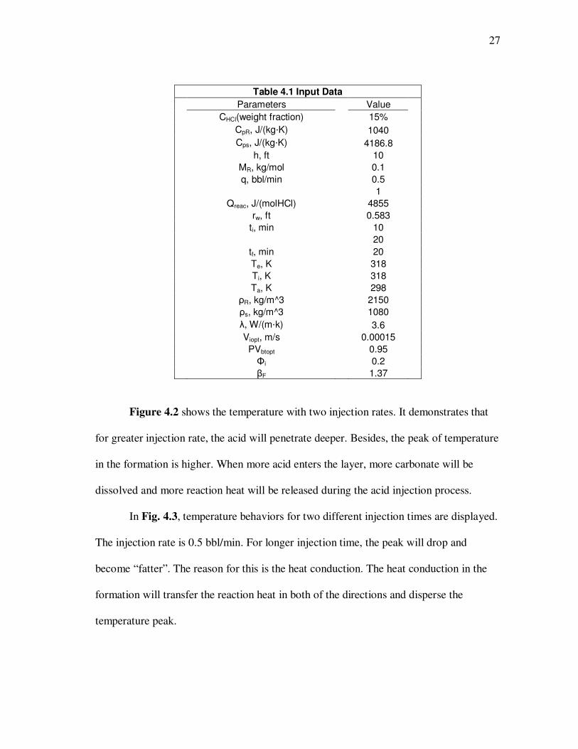
Figure 4.2 shows the temperature with two injection rates. It demonstrates that
for greater injection rate, the acid will penetrate deeper. Besides, the peak of temperature
in the formation is higher. When more acid enters the layer, more carbonate will be
dissolved and more reaction heat will be released during the acid injection process.
In Fig. 4.3, temperature behaviors for two different injection times are displayed.
The injection rate is 0.5 bbl/min. For longer injection time, the peak will drop and
become “fatter”. The reason for this is the heat conduction. The heat conduction in the
formation will transfer the reaction heat in both of the directions and disperse the
temperature peak.

28
295
300
305
310
315
320
325
330
335
0 0.5 1 1.5 2 2.5 3 3.5 4
Radius, ft
Te
mp
era
ture
, K
Fig. 4.1—Temperature distribution in the formation for q=1 bbl/min after injecting for 10 min
295
300
305
310
315
320
325
330
335
0 0.5 1 1.5 2 2.5 3 3.5 4
Radius, ft
Tem
pera
ture
, K
Fig. 4.2—Temperature distribution in the formation for different injection rate after injecting for 10 min
q=0.5bbl/min q=1bbl/min
1
2
3

29
295
300
305
310
315
320
325
330
0 0.5 1 1.5 2 2.5 3 3.5 4
Radius, ft
Tem
pera
ture
, K
Fig. 4.3—Temperature distribution in the formation for different injection time when q=0.5 bbl/min
Comparing Fig. 4.3 and Fig. 4.4, different injection rates give us different
velocities of acid, which affect the heat convection. Then the shape of the temperature
peak varies.
ti=20 min ti= 10 min

30
295
300
305
310
315
320
325
330
335
0 0.5 1 1.5 2 2.5 3 3.5 4
Radius, ft
Tem
pera
ture
, K
Fig. 4.4—Temperature distribution in the formation for different injection time when q=1 bbl/min
Wormhole front and spent acid front are presented in Fig. 4.5. The spent acid
front is ahead of the wormhole front in this case based on the optimum interstitial
velocity and the optimum breakthrough pore volumes we input to the model. The
breakthrough pore volumes calculated for each time step is greater than 1 as the reason
for that the spent acid front is ahead of the wormhole front. The break through pore
volumes is considered as a function of time, showing in Fig. 4.6. It decreases with time
since it is proportional to 3/1
iV . The wormhole efficiency, the volumetric fraction of
dissolved rock, also decreases with time (Fig. 4.7) for the reason that the acid is
consumed along the wormhole as it forms. When acid goes further and further, the
concentration of HCl decreases and wormhole efficiency decreases as well.
ti=10 min ti=20 min

31
0
0.5
1
1.5
2
2.5
3
3.5
4
4.5
0 5 10 15 20 25
Injection Time, min
rs &
rw
h,
ft
Fig. 4.5—Wormhole front and spent acid front when q= 1 bbl/min
1
1.5
2
2.5
3
3.5
4
0 5 10 15 20 25
Injection Time, min
PV
bt
Fig. 4.6—Break through pore volumes as a function of time greater than 1 when q=1 bbl/min
Spent acid front
Wormhole front

32
0.02
0.03
0.04
0.05
0.06
0.07
0.08
0.09
0.1
0 5 10 15 20 25
Injection Time, min
Worm
hole
Effic
iency
Fig. 4.7—Wormhole efficiency as a function of time when q=1 bbl/min
The average porosity of treated formation will increased first since the more pore
volume is created by reaction, which is shown as the first part of the curve in Fig. 4.8.
After that, since the wormhole efficiency decreases all the time, then the pore volume
created every time step by reaction decreases as well. Besides, the treated region is
increasing. However, the average porosity is still greater than the original porosity.
33
0.15
0.17
0.19
0.21
0.23
0.25
0.27
0 5 10 15 20 25
Injection Time, min
Ave
rag
e P
oro
sit
y
Fig. 4.8—Average porosity of treated formation as a function of time when q=1 bbl/min
4.3 Temperature Profile during Flowing Back
Using the temperature profile obtained in the acid injection problem as the initial
condition, we can simulate the temperature profile in the formation when the well is
flowing back.
Figure 4.9 shows that when the well is flowing back, the acid injected will enter
the well first, followed by the formation fluid with the geothermal temperature at this
depth. The temperature peak caused by reaction should arrive at the wellbore between
them in time.
If the injection rate and flow-back flow rate is higher, the temperature peak will
arrive at the wellbore faster, which is clearly shown comparing Fig. 4.9 and Fig. 4.10.

34
295
300
305
310
315
320
325
330
0 0.5 1 1.5 2 2.5 3 3.5 4
Radius, ft
Tem
pera
ture
, K
Fig. 4.9—Temperature profile in the formation when the well is flowing back at 0.5 bbl/min after injection for 10 min (0.5bbl/min)
295
300
305
310
315
320
325
330
335
0 0.5 1 1.5 2 2.5 3 3.5 4
Radius, ft
Tem
pera
ture
, K
Fig. 4.10—Temperature profile in the formation when the well is flowing back at 1 bbl/min after injection for 10 min (1 bbl/min)
t=0 min
t=1.7 min
t=3.3 min
t=0 min t=1.7 min
t=3.3 min

35
Figure 4.11 presents the temperature profile after injection for 20 min. With
longer injection time, the acid will penetrate deeper, and therefore it takes longer time to
flow the acid and temperature peak back to the wellbore. Besides, the temperature peak
is becoming wider because if the total reaction heat is constant, the radius range for
temperature peak is larger since this is a radial flow problem.
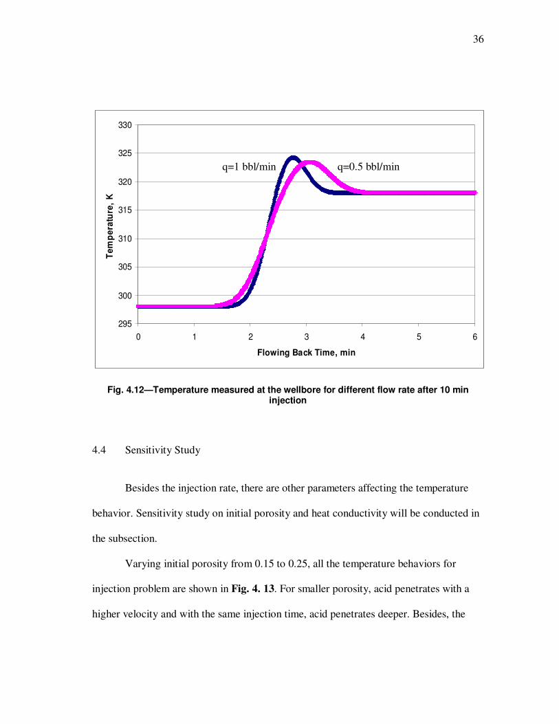
Figure 4.12 is plotting the wellbore temperature as a function of time. For
different injection rate, we have different wellbore temperature behavior, not only the
value of the peak, but also the time when the peak reaches the wellbore. All these
differences are caused by reaction, which gives us a mechanism to quantitatively
determine the acid flow profile.
295
300
305
310
315
320
325
330
0 0.5 1 1.5 2 2.5 3 3.5 4
Radius, ft
Tem
pera
ture
, K
Fig. 4.11—Temperature profile in the formation when the well is flowing back at 1 bbl/min after injection for 20 min (1 bbl/min)
t=0 min
t=3.3 min
t=5 min
36
295
300
305
310
315
320
325
330
0 1 2 3 4 5 6
Flowing Back Time, min
Te
mp
era
ture
, K
Fig. 4.12—Temperature measured at the wellbore for different flow rate after 10 min injection
4.4 Sensitivity Study
Besides the injection rate, there are other parameters affecting the temperature
behavior. Sensitivity study on initial porosity and heat conductivity will be conducted in
the subsection.
Varying initial porosity from 0.15 to 0.25, all the temperature behaviors for
injection problem are shown in Fig. 4. 13. For smaller porosity, acid penetrates with a
higher velocity and with the same injection time, acid penetrates deeper. Besides, the
q=1 bbl/min q=0.5 bbl/min

37
reaction region we assumed is larger which is going to be heated by reaction heat. That
is the reason we have lower peak for iφ =0.15.
295
300
305
310
315
320
325
330
335
0 0.5 1 1.5 2 2.5 3 3.5 4
Radius, ft
Te
mp
era
ture
, K
Φi=0.15
Φi=0.2
Φi=0.25
Fig. 4.13—Comparison of injection temperature profile for different porosity
For the flow-back problem (Fig. 4.14), since the flow-back velocity is also larger
for smaller porosity, the distance between three peaks decreases. Another thing need to
be noticed is that the temperature peak for the largest porosity is the lowest although
during injection it has the highest peak. This is caused by the reaction heat. For iφ =0.25,
the amount of rock that can be dissolved is small so that the reaction heat released is
small as well. During injection, this reaction heat only needs to heat up a small reaction

38
region and shows larger temperature increase. During flowing back, the peak will be
reduced because the small amount of reaction heat.
295
300
305
310
315
320
325
330
0 1 2 3 4 5 6
Flow Back Time, min
Te
mp
era
ture
, K
Φi=0.15
Φi=0.2
Φi=0.25
Fig. 4.14—Comparison of wellbore temperature profile for different porosity
From Fig. 4.15 and Fig. 4.16, we can see that heat conductivity for both rock and
solution does not have great effect on the temperature behavior. Only the height of the
peak changes a little because more heat is dispersed by heat conduction. This also proves
that heat convection is dominating in this heat transfer process.

39
295
300
305
310
315
320
325
330
335
0 0.5 1 1.5 2 2.5 3 3.5 4
Radius, ft
Te
mp
era
ture
, K
λ=3.6 W/(mK)
λ=4.8 W/(mK)
λ=6.0 W/(mK)
Fig. 4.15—Comparison of injection temperature profile for different heat conductivity
295
300
305
310
315
320
325
330
0 1 2 3 4 5 6
Flow Back Time, min
Te
mp
era
ture
, K
λ=3.6 W/(mK)
λ=4.8 W/(mK)
λ=6 W/(mK)
Fig. 4.16—Comparison of wellbore temperature profile for different heat conductivity

40
Figure 4.17 shows the sensitivity of wellbore temperature to the injection rate.
The flow-back rate is assumed the same as injection rate. We observe that for just a little
change of the injection rate, we have obvious deviation of the temperature behavior. This
gives us more confidence for the future work.
295
300
305
310
315
320
325
330
0 1 2 3 4 5 6
Flow Back Time, min
Tem
pera
ture
, K
q=0.2 bbl/min
q=0.4 bbl/min
q=0.6 bbl/min
q=0.8 bbl/min
q=1 bbl/min
Fig. 4.17—Comparison of wellbore temperature profile for different injection rate
4.5 Section Summary
In this section, we showed the results for injection problem and flow-back
problem. For injection problem, we have three parts of the curve: acid temperature,
reaction peak and geothermal temperature. For flow-back problem, we still have these
three parts and peak disperses with time. The most significant thing is we have different

41
temperature behaviors for different injection rates and this provide us a method to
quantify the acid flow profile.

42
5. CONCLUSIONS AND RECOMMENDATIONS
5.1 Conclusions
Combining the energy balance equation, Buijse’s wormhole model and modified
volumetric wormhole model, we developed a new model to simulate the heat transfer
process in the formation during acid injection and flowing back. Heat conduction, heat
convection and reaction heat are all considered. With this model, it was found:
• Reaction has significant effects on the temperature profile in the formation and
wellbore temperature behavior. Reaction heat will form a temperature peak easy
to identify since it is between cool acid temperature and geothermal temperature.
• The wellbore temperature behavior is sensitive to the acid injection rate,
providing us a mechanism to determine the acid injection profile quantitatively.
This also gives us confidence for future work.
5.2 Recommendations and Future Work
We have only single layer model in this research. However, the model should be
developed for multilayer formation.
Besides, the inverse model should be developed to obtain the acid flow profile
from the temperature data measured by DTS.
There are still some aspects of the model we can improve. For acid injection
problem, we assume that the reaction only occurs at the front of wormholes. As a matter

43
of facts, many branches form with the main wormhole and reaction also happens at the
branches. More accurate wormhole model may be used here.
In the flow-back problem, we neglected the heat conduction term in the energy
balance equation because the heat convection is dominating. However, at the location of
temperature peak, the temperature gradient is large, in other words, the heat conduction
is important at this location.
In this research, the whole approach should include forward model and inverse
model. Here we just developed part of the forward model which is a 1-D model. 2-D
formation model can be developed with the consideration of the height of each layer.
Wellbore thermal model should be developed and coupled with the model we
already had. The heat transfer in the wellbore will also affect the temperature behavior in
the wellbore significantly.

44
NOMENCLATURE
Symbol Description
0
HClC = concentration of HCl, weight fraction, dimensionless
Cps = heat capacity of acid solution, m/Lt2T, J/(kg·K)
CpR = heat capacity of rock, m/Lt2T , J/(kg·K)
ek = specific kinetic energy of acid solution, m/Lt2, J/kg
ep = specific potential energy of acid solution, m/Lt2, J/kg
eR = specific internal energy of rock, m/Lt2, J/kg
es = specific internal of acid solution, m/Lt2, J/kg
Eaccu = energy accumulating in the element, m2/Lt
2, J
Ecreated = energy created in the element, m2/Lt
2, J
Ein = energy flowing into the element, m2/Lt
2, J
Eout = energy flowing out of the element, m2/Lt
2, J
h = height of the layer, L, m [ft]
H = enthalpy of substance, L2T
2, J/mol [kcal/mol]
H = specific enthalpy of acid solution, m/Lt2, J/kg
m = counter of grid block, dimensionless
MR = molecular mass of rock, kg/mol
nHClcon = mole of consumed HCl, mol
NAC = acid capacity number, dimensionless
p = counter of time step, dimensionless

45
P = pressure, m/Lt2, Pa
PVbt = break through pore volumes, dimensionless
PVbtopt = optimum break through pore volumes, dimensionless
q = injection rate of acid solution, L3/t, m
3/s [bbl/min]
''q = heat flux caused by heat conduction, m/t3, W/m
2
Q = volume of injected acid, L3, m
3 [bbl]
Qreac = reaction heat released by unit mole HCl, m2/Lt
2, J/(molHCl)
r = radius, L, m
rw = wellbore radius, L, m [ft]
Rs = radius of spent acid front, L, m
Rwh = radius of wormhole front, L, m
t = time, t, s
tf = total flow back time, t, s
ti = total injection time, t, s
T = temperature, T, K
Ta = temperature of acid injected, T, K
Tg = geothermal temperature, T, K
Ti = initial temperature of reservoir, T, K
u = velocity of acid solution, L/t, m/s
uw = velocity of acid solution at wellbore radius, L/t, m/s
v = specific volume, L3/m, m
3/kg
Vdis = volume of dissolved rock, L3, m
3

46
0
FV = volumetric fraction of fast-reacting rock, dimensionless
Vi = interstitial velocity, L/t, m/s [cm/min]
Viopt = optimum interstitial velocity, L/t, m/s [cm/min]
Vwh = velocity of wormhole growth, L/t, m/s [cm/min]
WB = constant in wormhole model, (L/t)-2
, (m/s)-2
Weff = constant in wormhole model, (L/t)1/3
, (m/s)1/3
Wt = time delay constant, t, s
z = coordinate in height direction of the layer, L, m
Greek
βF = dissolve power of acid, weight fraction, dimensionless
η = wormhole efficiency, volumetric fraction, dimensionless
λ = heat conductivity of acid solution and rock, mL/t3T, W/(m·K)
ρR = density of rock, m/L3, kg/m
3
ρs = density of acid solution, m/L3, kg/m
3
φ = porosity, volumetric fraction, dimensionless
iφ = initial porosity, volumetric fraction, dimensionless
∆ = prefix for difference
Subscript
a = acid
con = consumed
dis = dissolved
F = fast reaction
47
i = initial
opt = optimum
R = rock
s = acid solution
w = well
wh = wormhole

48
REFERENCES
Buijse, M. and Glasbergen, G.: “A Semiempirical Model to Calculate Wormhole
Growth in Carbonate Acidizing,” paper SPE 96892 presented at the 2005 SPE
Annual Technical Conference and Exhibition, Dallas, Texas, 9-12 October.
Clanton, R.W., Haney, J.A., Pruett, R., Wahl, C.L., Goiffon, J.J. and Gualtieri, D.:
“Real-Time Monitoring of Acid Stimulation Using a Fiber-Optic DTS System,”
paper SPE 100617 presented at the 2006 SPE Western Regional/AAPG Pacific
Section/GSA Cordilleran Section Joint Meeting, Anchorage, Alaska, 8-10 May.
Economides, M.J., Hill, A.D. and Ehlig-Economides, C.: Petroleum Production
System, 400. 1993. Upper Saddle River, New Jersey: Prentice Hall, Inc.
Gao, G. and Jalali, Y.: “Interpretation of Distributed Temperature Data during
Injection Period in Horizontal Wells,” paper SPE 96260 presented at the 2005 SPE
Annual Technical Conference and Exhibition, Dallas, Texas, 9-12 October.
Glasbergen, G., Gualtieri, D., Domelen, M.V. and Sierra, J.: “Real-Time Fluid
Distribution Determination in Matrix Treatments Using DTS,” paper SPE 107775
presented at the 2007 European Formation Damage Conference, Scheveningen, The
Netherlands, 30 May- 1 June.

49
Johnson, D., Sierra, J., Kaura, J., and Gualtieri, D.: “Successful Flow Profiling of
Gas Wells Using Distributed Temperature Sensing Data,” paper SPE 103097
presented at the 2006 SPE Annual Technical Conference and Exhibition, San
Antonio, Texas, 24-27 September.
Medeiros, F. and Trevisan, O.V.: “Thermal Analysis in Matrix Acidization,” Journal
of Petroleum Science and Engineering, 2006. 51: 85-96.
Perry, R.H., Green, D.W. and Maloney, J.O: Perry’s Chemical Engineers’
Handbook, 226-231. 1963. New York: McGraw-Hill Book Co.
Wang, X., Lee, J., Thigpen, B., Vachon, G., Poland, S. and Norton, D.: “Modeling
Flow Profile using Distributed Temperature Sensor (DTS) System,” paper SPE
111790 presented at the 2008 SPE Intelligent Energy Conference and Exhibition,
Amsterdam, The Netherlands, 25-27 February.
Whitson, C.H. and Kuntadi, A.: “Khuff Gas Condensate Development,” paper SPE
10692 presented at the 2005 International Petroleum Technology Conference, Doha,
Qatar, 21-23 November.
Yoshioka, K., Zhu, D., and Hill, A.D.: “A New Inversion Method to Interpret Flow
Profiles from Distributed Temperature and Pressure Measurements in Horizontal

50
Wells,” paper SPE 109749 presented at the 2007 SPE Annual Technical Conference
and Exhibition, Anaheim, California, 11-14 November.

51
VITA
Name: Xuehao Tan
Address: Lifeng 5#, Zhanqian District
Yingkou, Liaoning,
115000, China
Email Address: [email protected]
Education: B.E., Engineering Thermal Physics, Tsinghua
University, 2007
M.S. Petroleum Engineering, Texas A&M
University, 2009
This thesis was typed by the author.