Predicting gully initiation: comparing data mining ... et al... · techniques, analytical hierarchy processes and the ... which is substantially lower in agricultura l fields, while

EARTH SURFACE PROCESSES AND LANDFORMSEarth Surf. Process. Landforms 37, 607–619 (2012)Copyright © 2012 John Wiley & Sons, Ltd.Published online 1 January 2012 in Wiley Online Library(wileyonlinelibrary.com) DOI: 10.1002/esp.2273

Predicting gully initiation: comparing data miningtechniques, analytical hierarchy processes and thetopographic thresholdTal Svoray,1* Evgenia Michailov,2 Avraham Cohen,2 Lior Rokah2 and Arnon Sturm2

1 Department of Geography and Environmental Development, Ben-Gurion University of the Negev, Beer-Sheva 84105, Israel2 Department of Information Systems Engineering, Ben-Gurion University of the Negev, Beer-Sheva 84105, Israel

Received 23 March 2011; Revised 6 November 2011; Accepted 17 November 2011

*Correspondence to: T. Svoray, Department of Geography and Environmental Development, Ben-Gurion University of the Negev, Beer-Sheva 84105, Israel.E-mail: [email protected]

ABSTRACT: Predicting gully initiation at catchment scale was done previously by integrating a geographical information system(GIS) with physically based models, statistical procedures or with knowledge-based expert systems. However, the reliability andvalidity of applying these procedures are still questionable. In this work, a data mining (DM) procedure based on decision treeswas applied to identify areas of gully initiation risk. Performance was compared with the analytic hierarchy process (AHP) expertsystem and with the commonly used topographic threshold (TT) technique. A spatial database was used to test the models, composedof a target variable (presence or absence of initial points) and ten independent environmental, climatic and human-inducedvariables. The following findings emerged: using the same input layers, DM provided better predictive ability of gully initiation pointsthan the application of both AHP and TT. The main difference between DM and TT was the very high overestimation inherent in TT. Inaddition, the minimum slope observed for soil detachment was 2�, whereas in other studies it is 3�. This could be explained by soil resistance,which is substantially lower in agricultural fields, while most studies test unploughed soil. Finally, rainfall intensity events >62.2mmh-1

(for a period of 30min) were found to have a significant effect on gully initiation. Copyright © 2012 John Wiley & Sons, Ltd.

KEYWORDS: AHP; data mining; ephemeral gullies; GIS; land degradation; topographic threshold

Introduction

Erosion processes in agricultural fields can cause majorenvironmental damage through soil loss (Trimble and Crosson,2000; Van Rompaey et al., 2003). Since the mid-1980s, muchattention has been given to understanding and predicting gullyinitiation (Cheng et al., 2006), which, of all erosion processes,is now regarded as one of the most destructive mechanismsaffecting agricultural soils (De-Santisteban et al., 2006). Gullyerosion represents an important – if not the dominant – sedimentsourcewithin catchments, while the gullies themselves constituteeffective links for transferring runoff, sediment and othermaterialsfrom source to sink. They thereby have an important role inincreasing connectivity on the landscape scale (Casali et al.,2009). This is probably the reason for making an effort in recentyears to use field measurements, as well as numerical modelsimulations, to study gully processes and gully dynamics (Kirkbyand Bracken, 2009). Special attention has been given in previousresearch to the following questions: What causes gully initiation?Where it ismost likely to occur? Andwhat can be done to preventgully creation?There are several ways to predict gully initiation using, mainly,

physically based models. However, in recent years, variouscomputer-supported methods have been used to predict gullyoccurrence. Among the several computational methods, there

are two, very different approaches to predict gullying:(1) systems based on expert knowledge and experience; and(2) empirical methods.

An expert-based system enables human experts to integrateand translate their quantitative and qualitative knowledge intocomputer language, using formal and controlled procedures(Malczewski, 2004). The method assumes that the expertunderstands the mechanisms studied and that his knowledgecan be translated accurately into computer language. Amongexpert-based methods, the most intuitive are the analyticalhierarchy process (AHP) mechanisms (Saaty, 1977; Malczewski,1999). In general, a typical AHP includes two main procedures:scoring and interpolating. Pairwise comparison is an advancedscoring method for examining real-world conditions in arelatively reliable way. Using this method, a matrix is developedin which every criterion is accorded a value based on itsimportance in relation to all other criteria and the weight of eachcriterion’s relative importance is calculated. Once the weights ofimportance for each criterion are established, the variables canbe combined and interpolated over the entire study area.

Methods of interpolating AHPs can be classified into twomain groups based on the level of analysis required fromdecision-makers and experts and according to the methods ofranking and developing weights per variable. The firstgroup includes compensatory methods, in which a scale of

608 T. SVORAY ET AL.

adjustment levels and index weights that compensate oneanother is used. The compensatory approach is demanding,since it requires that decision-makers and experts place therange of criteria on a scale according to specific adjustmentlevels in addition to developing each criterion’s weight. In thesecond group, which includes non-compensatory methods,the comparison between the alternatives (land use, for example)is carried out with no option of alternating and compensatingbetween the internal scale (the range of criterion values) andthe weights of each criterion. Entailing, at most, only a serialranking of the criteria, this approach requires less attention fromdecision-makers and ranking experts (Jankowski, 1995).Weighted linear combination (WLC) is a common compensa-

tory method for estimating and implementing numerous criteriain a geographical information system (GIS). This method simplycombines successive variables on a linear basis, forming pointsof adaptability for specific purposes. In spatial studies, AHPanalyses, combined with GIS, have improved the ability ofclassic multi-layered analysis and process- based models (Collinset al., 2001) to predict spatial phenomena. Thus, the method hasfound its way into many fields of decision-making, such asforestation (Gilliams et al., 2005). Furthermore, AHP has beenwidely used in such fields as engineering geology (Dai et al.2001) and geomorphology (Ni and Li, 2003; Ni et al. 2008;Svoray and Ben-Said, 2010). However, although previous studiesshow the potential of AHP in geomorphology, several aspects ofAHP require further elucidation: the reliability of the experts andof the knowledge mining procedures and algorithms applied tointerpolate the predictions in space.On the other hand, a purely empirical method – the topo-

graphic threshold (TT) method – can predict the threshold valueof initiation based on data of observed gully initiation points. Sev-eral studies of the slope and area required to support channel headincision have found that an inverse relationship exists between theupslope contributing area and the local slope in different environ-ments (Montgomery and Dietrich, 1988; Hancock and Evans,2006; Svoray andMarkovitch, 2009). According to this approach,runoff volumemay increase proportionally to catchment area andgully erosion may take place where the threshold value predictedby the empirical TT is exceeded. Although the TT method is com-monly used, several studies have found that it may induce errorsin predicting gully initiation (Chaplot et al., 2005).Amore complex empirical method is the knowledge discovery

database (KDD) method, which is established mathematically onthe basis of data mining (DM) techniques. KDD is the process ofidentifying valid, novel, useful, and understandable patterns fromlarge datasets (Fayyad et al., 1996). With the ever-increasing rateof data accumulation, KDD is becoming an important tool fortransforming this data into useful information. KDD techniqueshave been used in geomorphological studies, for example forlandslide susceptibility zonation (Melchiorre et al., 2008); forevaluating sedimentation vulnerability (Hentati et al., 2010); todetermine land stability (Pavel et al., 2008) and to study gullyinitiation (Gutierrez et al., 2009a). Data mining is the mathemati-cal core of the KDD process (Maimon and Rokach, 2005),involving the inference of algorithms that explore the data,develop mathematical models and discover significant patterns(implicit or explicit) –which are the essence of useful knowledge.In general, DM includes three stages: the first, the pre-processingstage includes data assemblage, cleaning and division intotraining and validation sets. The second step involves the actualDM algorithms and the final third step includes validation ofthe results in relation to observations.DM can be used for various tasks such as classification,

clustering and regression. Here, we focus on a binary classifica-tion task, where the goal is to classify points into either ‘gullyinitial point’ or ‘non-gully initial point’. In a typical classification

Copyright © 2012 John Wiley & Sons, Ltd.

task, a training set of labelled examples is given and the goal is toform a description that can predict previously unseen examples.An inducer aims to build a classifier (also known as a classifica-tion model), by learning from a set of pre-classified instances.The classifier can then classify unlabelled instances.

When acquiring new information, the expert and empiricalapproaches rely on different paradigms. Whereas the formerapproach is based on mining processed knowledge that maynot be derived from field measurements of the studied area, thelatter extracts information based on a well-defined database ofmeasurements whose size determines the validity of the results.It is quite clear that the two methods are imperfect and eachhas its advantages and disadvantages. Regarding the expert-based approach, various questions naturally arise: Who areexperts? How reliable are they? Do they understand the underly-ing mechanisms? In addition there are objective factors such asthe fact that the method of translating knowledge into computerlanguage, that is often qualitative, is not fully understood. Finally,human expertise is a scarce resource that is not always available.All the above difficulties are known as the ‘knowledge acquisi-tion bottleneck’. The empirical approach also raises several ques-tions. How representative is the database? How large does such adatabase need to be? Andwhat canwe infer about the underlyingmechanisms from the complex statistical process?

The fact that the two approaches, despite their limitations, havebeen found useful for understanding geomorphological and soilerosion processes, calls for a quantitative comparison. The aimsof this study are therefore: (1) to apply a data mining techniqueto predict gully initiation points in an agricultural catchment;(2) to compare the model results with predictions made by AHPand the TT; and (3) to study the rules generated by the dataminingprocedure to better understand what causes gully incision.

The Study Area

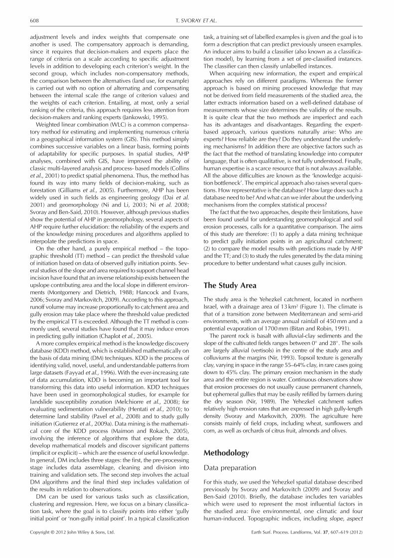
The study area is the Yehezkel catchment, located in northernIsrael, with a drainage area of 13km² (Figure 1). The climate isthat of a transition zone between Mediterranean and semi-aridenvironments, with an average annual rainfall of 450mm and apotential evaporation of 1700mm (Bitan and Robin, 1991).

The parent rock is basalt with alluvial-clay sediments and theslope of the cultivated fields ranges between 0� and 28�. The soilsare largely alluvial (vertisols) in the centre of the study area andcolluviums at the margins (Nir, 1993). Topsoil texture is generallyclay, varying in space in the range 55–64%clay, in rare cases goingdown to 45% clay. The primary erosion mechanism in the studyarea and the entire region is water. Continuous observations showthat erosion processes do not usually cause permanent channels,but ephemeral gullies that may be easily refilled by farmers duringthe dry season (Nir, 1989). The Yehezkel catchment suffersrelatively high erosion rates that are expressed in high gully-lengthdensity (Svoray and Markovitch, 2009). The agriculture hereconsists mainly of field crops, including wheat, sunflowers andcorn, as well as orchards of citrus fruit, almonds and olives.

Methodology

Data preparation

For this study, we used the Yehezkel spatial database describedpreviously by Svoray and Markovitch (2009) and Svoray andBen-Said (2010). Briefly, the database includes ten variableswhich were used to represent the most influential factors inthe studied area: five environmental, one climatic and fourhuman-induced. Topographic indices, including slope, aspect

Earth Surf. Process. Landforms, Vol. 37, 607–619 (2012)

Beer Sheva

Jord

an R

iver

KfarYehezkel

Afula

She’anBeit

Figure 1. The study area. A shaded relief map of the Yehezkel catchment in Israel.

609PREDICTING GULLY INITIATION: A COMPARATIVE STUDY

and the upslope contributing area, were calculated from adigital elevation model (DEM). The contour-based DEM wasextracted from a triangulated irregular network (TIN), createdfrom a digital topographic map with 5-meter intervals thatwas prepared by the Survey of Israel. Each 1.5� 1.5m2 cellin the catchment was assigned an elevation value ranging from(�15) to (+495). The DEM was tested against field measure-ments and high correlation was achieved between the pre-dicted elevation values and actual measurements (r2 = 0.90;n = 20; p< 0.0001). Vertical accuracy was found to beapproximately 5m and the positional accuracy was better than1.3m. All artificial pits were removed from the DEM (Tarbotonet al., 1989) and slope and flow accumulation were calculatedper cell, using TauDEM Dinf (Tarboton, 1997). To map as inputthe study area’s vegetation, rock and soil cover, maximumlikelihood classification was used with an orthophoto withspatial resolution 0.4� 0.4m2, acquired on November 2006under clear sky conditions. To calculate the cover percentageof these classes, the ArcGIS workstation Fishnet operationwas used to produce 25� 25-m2 continuous cells coveringthe entire study area. Spatial representation of rainfall intensitywas applied by using meteorological radar data that coveredthe entire study area during a rainfall event (28/10/2006), witha return period of 20 years. From the 2006 aerial photo andbased on visual interpretation, tillage direction was digitizedfor all fields of the watershed. To express the effect of tillagedirection on gully initiation, we used a cosine function. Aland-usemap with spatial resolution of 2� 2m2 was compiled,based on data from the National GIS of Israel, made by theSurvey of Israel. Unpaved roads were manually digitized fromthe 2006 orthophoto, based on visual interpretation. As derivedfrom expert recommendations, the roads layer was divided intotwo criteria (occupying two separate GIS layers): (1) roads-as-runoff-contributors enhancing the effect of roads on thecontributing area downslope; and (2) roads-as-barriers to waterponding and sediment logging, enhancing the effect of roads as


barriers to water and sediment flow from upslope. The cells in thetwo layers were coded according to their distance from the road.

Since one of the goals of this paper was to compare a DMapproach to existing AHP and TT methods, we based our analysison the same dataset for each one of the methods. In particular,when comparing the AHP approach, we used for validation only32 gully initiation points, observed in the 2006 airphoto. The fea-ture set for the comparison with AHP included four integer vari-ables (slope, land use, aspect, and upslope contributing area);four double variables (tillage direction, rock, rainfall intensity andvegetation cover) and one enumeration variable (unpaved roads).In our comparison with the TT model, we used only 19 physicallymeasured gully initiation points as a training set and 113 digitizedpoints, observed in the 2006 airphoto, as a validation set. Onlytwo features were included in the comparison with the TT tech-nique: slope (integers) and upslope contributing area (integers).

The data mining procedure

The use of KDD to study gullying is not trivial since the classifica-tion problem of whether a given cell is likely to include a gullyinitiation point or not involves several methodological chal-lenges, primarily the ‘rare cases’ challenge (Weiss, 2010). Theobserved data in this study consist of 113 detected gully initiationpoints, versus millions of other raster cells within the catchmentwithout gully initiation points. In the study of gully initiation, thisis a typical phenomenon in many eroded catchments; the num-ber of cells with initiation points is very much smaller than thenumber of cells without them. In such cases, there is a highchance that an overly simple classifier may classify all points inquestion as ‘no gully initiation point’. This problem is not limitedto gullies as a phenomenon, or even to geomorphology, butconfronts classifiers in all fields of study. For a variety of reasons,rare cases pose difficulties for induction algorithms (Weiss, 2010).The most obvious and fundamental problem is the associated


0

0.91

0.905

0.90

0.895

0.89

0.885

0.88

0.875

Ratio

Are

a un

der

the

RO

C c

urve

10 20 300 40 50 60 70 9080 100 110 120 140 150130

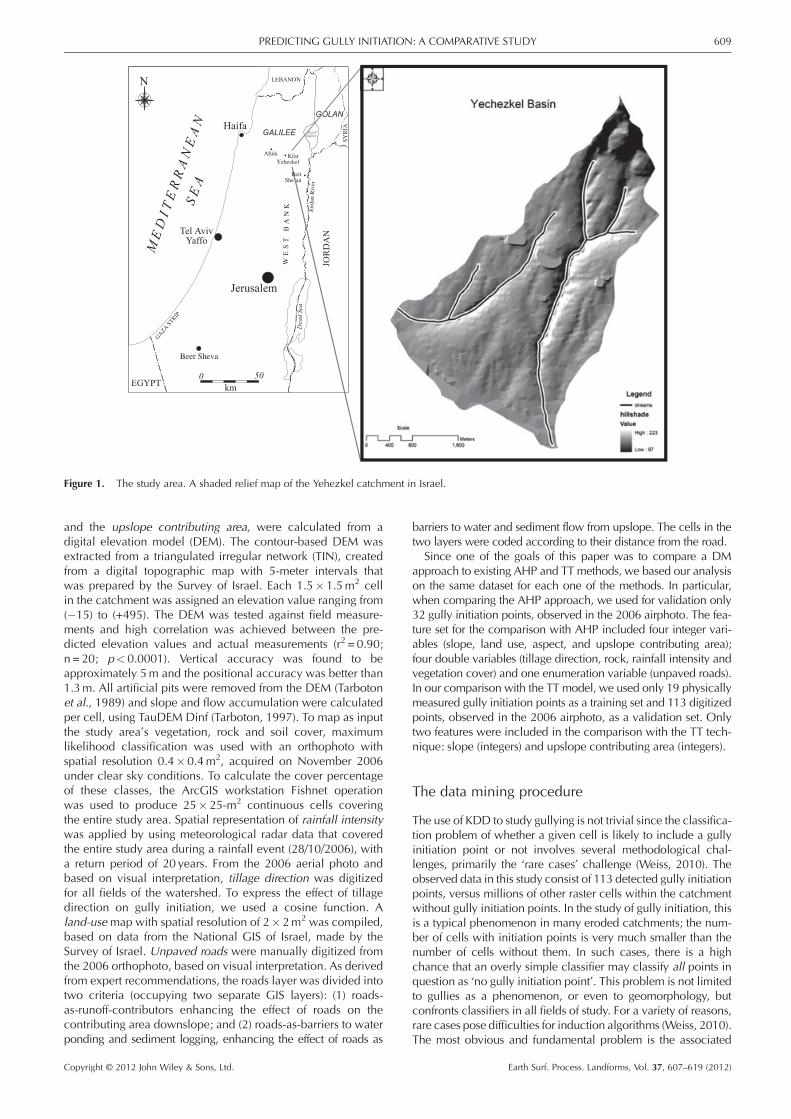
Figure 3. The area under the ROC curve for several ratio values (no-


lack of data – rare cases tend to cover only a few trainingexamples (i.e. absolute rarity). This lack of data hampers thedetection of the rare cases and, even if a rare case is detected, itmakes generalization difficult, since it is hard to identifyregularities from only a few data points. This problem is usuallyreferred to in the literature as prevalence (different proportionsof presence/absence observations in the dataset). Beguería(2006) has shown that prevalence raises the need to usethreshold independent statistics such as the receiver operatingcharacteristics (ROC) curve for the validation of predictivemodels. In particular, Gutiérrez et al. (2009b) analyse the roleof prevalence in the success of decision trees to model thedistribution of gullies. They conclude that there is no influenceon the success of the models, when the training set includes asufficiently large number of observations (approximately 500presences and 2000 absences).Another problem associated with mining rare cases is reflected

by the phrase: like a needle in a haystack. The difficulty is not somuch due to the needle being small – or there being only oneneedle – but by the fact that the needle is obscured by a hugenumber of strands of hay. Similarly, in data mining, rare casesmay be obscured by common cases (relative rarity). This isespecially a problem when data mining algorithms rely on whatare called ‘greedy search heuristics’ that examine one variableat a time as in the case of classification trees (Rokach andMaimon, 2008). With greedy algorithms, rare cases may dependon the conjunction of many conditions and any single conditionin isolation may not provide much guidance.Another challenge is that the predictive accuracy of a classi-

fier alone is insufficient as an evaluation criterion. One reasonfor this phenomenon is that various validation and classifica-tion errors must be dealt with differently. More specifically,false negative errors, i.e., mistaking ‘gully’ for ‘non-gully’, areless desirable than false positive errors. Moreover, predictiveaccuracy alone does not provide enough flexibility whenselecting a target for gully initiation. For example, the personnelmay want to examine 1% of the available potential points, butthe model predicts that only 0.1% of them are gully points. Toresolve the issue of rare cases, then, we need to use other vali-dation measures, as discussed in the Validation section below.Figure 2 specifies the training process used for applying the

general data mining procedure.Given the collected set of gully initiation points (step 0), we

added, in step 1, random points (which are not gully initiationpoints) in an attempt to convert the problem into a binaryclassification task that can be solved with existing algorithms.The number of these points was of a magnitude of 100, with

Positive Gullies Incision Points

Extending the Database with

Random Negative Points

Multiple Balanced Datasets

Inducer

Inducer

Inducer

Classifier 1

Classifier 2

Classifier n

Figure 2. Outline of the training phase given only positive points.First, randomly selected negative points are added to the dataset. Thenmultiple balanced datasets are created. The dataset is used to train aclassifier and inducer.


respect to the number of gully initiation points. In a preliminarystudy, we examined the predictive performance (measured bythe area under the ROC curve) for several ratio values startingfrom 10 to 150 with steps of 10 using Adaboost-J48 as theclassification algorithm. As can be seen in Figure 3, the areaunder the curve (AUC) increases with the ratio. The processconverges approximately at a ratio of 90.

To address the rare cases challenge, we converted the datasetinto multiple balanced datasets (step 2). An inducer was executedon each balanced dataset (step 3) and a single classifier was gen-erated for each balanced dataset. Combining all classifiers from alldatasets constitutes an ‘ensemble of classifier’ (Rokach, 2010).Note that each member of the ensemble was trained separatelyover a dataset that includes all detected gully initiation pointsand an equivalent set of randomly selected points with no gullyinitiation points. By doing so, each classifier was trained over abalanced dataset. Moreover, in a preliminary study we tried tobuild an Adaboost-J48 classifier without splitting the data into abalanced dataset. However, we obtained poor results (an AUCof only 0.639). The incompatibility with previous results ofGutiérrez et al. (2009b) may be explained by the fact that in thisresearch we have only 32 presence points while in the previousresearch several hundred presence points were employed.

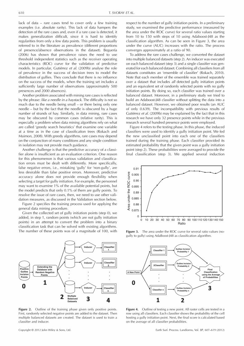
Figure 4 refers to the testing phase. In this phase, the inducedclassifiers were used to identify a gully initiation point. We fedthe new unclassified point into each one of the classifierstrained during the training phase. Each classifier provided itsestimated probability that the given point was a gully initiationpoint (step 2). These probabilities were averaged to provide thefinal classification (step 3). We applied several induction

gully to gully) using AdaBoost-J48 as classification algorithm.

A New Point

Gullies Incision Probability 1

Classifier 1

2Classifier

Classifier n

Gullies Incision Probability 2

Gullies Incision Probability n

Final Classification

using the Average of Probabilities

Figure 4. Outline of testing a new point. All raster cells are tested in arow using all classifiers. Each classifier shows the probability of the cellhosting a gully initiation point. Next, the final score is calculated basedon the average of all classifier probabilities.



algorithms to find the best that suited the nature of the dataset.We selected five techniques for evaluating the data. Below, weprovide a short explanation about each technique and thereasons for its selection.The decision tree algorithm (Quinlan, 1993) is a well-

established family of learning algorithms. Decision trees (orclassification trees) are used to classify an object (geographicalpoints in our case) to a predefined set of classes (gully/non-gully initiation points) based on its feature values (such astillage direction and rainfall intensity). The decision treecombines the features in a hierarchical fashion such that themost important feature is located in the root of the tree. Eachnode in the tree refers to one of the features. Each leaf isassigned to one class (gully/non-gully initiation points)representing the most frequent class value. In addition, the leafholds a probability vector indicating the probability of havinggully initiation points. New points are classified by navigatingthem from the root of the tree down to a leaf, according tothe outcome of the tests along the path.Decision trees assume that the feature space should be

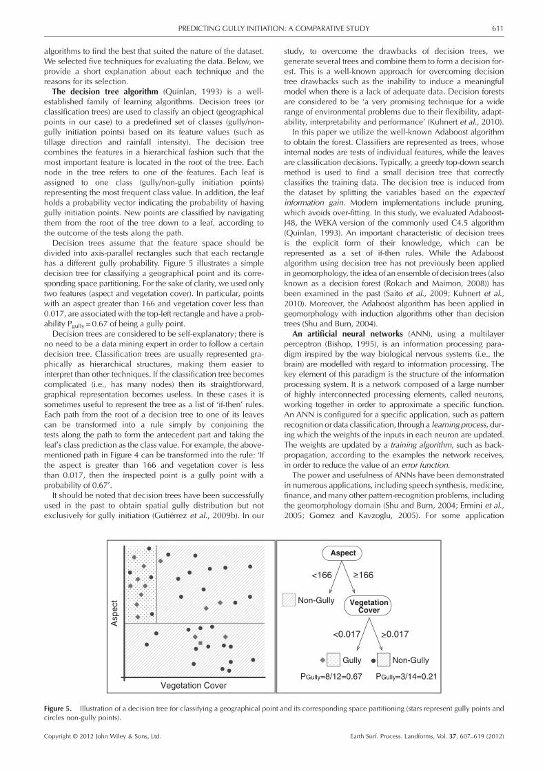
divided into axis-parallel rectangles such that each rectanglehas a different gully probability. Figure 5 illustrates a simpledecision tree for classifying a geographical point and its corre-sponding space partitioning. For the sake of clarity, we used onlytwo features (aspect and vegetation cover). In particular, pointswith an aspect greater than 166 and vegetation cover less than0.017, are associated with the top-left rectangle and have a prob-ability Pgully = 0.67 of being a gully point.Decision trees are considered to be self-explanatory; there is

no need to be a data mining expert in order to follow a certaindecision tree. Classification trees are usually represented gra-phically as hierarchical structures, making them easier tointerpret than other techniques. If the classification tree becomescomplicated (i.e., has many nodes) then its straightforward,graphical representation becomes useless. In these cases it issometimes useful to represent the tree as a list of ‘if-then’ rules.Each path from the root of a decision tree to one of its leavescan be transformed into a rule simply by conjoining thetests along the path to form the antecedent part and taking theleaf’s class prediction as the class value. For example, the above-mentioned path in Figure 4 can be transformed into the rule: ‘Ifthe aspect is greater than 166 and vegetation cover is lessthan 0.017, then the inspected point is a gully point with aprobability of 0.67’.It should be noted that decision trees have been successfully

used in the past to obtain spatial gully distribution but notexclusively for gully initiation (Gutiérrez et al., 2009b). In our

Asp

ect

Vegetation Cover

Figure 5. Illustration of a decision tree for classifying a geographical point acircles non-gully points).


study, to overcome the drawbacks of decision trees, wegenerate several trees and combine them to form a decision for-est. This is a well-known approach for overcoming decisiontree drawbacks such as the inability to induce a meaningfulmodel when there is a lack of adequate data. Decision forestsare considered to be ‘a very promising technique for a widerange of environmental problems due to their flexibility, adapt-ability, interpretability and performance’ (Kuhnert et al., 2010).

In this paper we utilize the well-known Adaboost algorithmto obtain the forest. Classifiers are represented as trees, whoseinternal nodes are tests of individual features, while the leavesare classification decisions. Typically, a greedy top-down searchmethod is used to find a small decision tree that correctlyclassifies the training data. The decision tree is induced fromthe dataset by splitting the variables based on the expectedinformation gain. Modern implementations include pruning,which avoids over-fitting. In this study, we evaluated Adaboost-J48, the WEKA version of the commonly used C4.5 algorithm(Quinlan, 1993). An important characteristic of decision treesis the explicit form of their knowledge, which can berepresented as a set of if-then rules. While the Adaboostalgorithm using decision tree has not previously been appliedin geomorphology, the idea of an ensemble of decision trees (alsoknown as a decision forest (Rokach and Maimon, 2008)) hasbeen examined in the past (Saito et al., 2009; Kuhnert et al.,2010). Moreover, the Adaboost algorithm has been applied ingeomorphology with induction algorithms other than decisiontrees (Shu and Burn, 2004).

An artificial neural networks (ANN), using a multilayerperceptron (Bishop, 1995), is an information processing para-digm inspired by the way biological nervous systems (i.e., thebrain) are modelled with regard to information processing. Thekey element of this paradigm is the structure of the informationprocessing system. It is a network composed of a large numberof highly interconnected processing elements, called neurons,working together in order to approximate a specific function.An ANN is configured for a specific application, such as patternrecognition or data classification, through a learning process, dur-ing which the weights of the inputs in each neuron are updated.The weights are updated by a training algorithm, such as back-propagation, according to the examples the network receives,in order to reduce the value of an error function.

The power and usefulness of ANNs have been demonstratedin numerous applications, including speech synthesis, medicine,finance, andmany other pattern-recognition problems, includingthe geomorphology domain (Shu and Burn, 2004; Ermini et al.,2005; Gomez and Kavzoglu, 2005). For some application

Aspect

<166

Non-Gully

Non-GullyGully

VegetationCover

>166

<0.017 >0.017

PGully=8/12=0.67 PGully=3/14=0.21

nd its corresponding space partitioning (stars represent gully points and



domains, neural models show more promise in achievinghuman-like performance than do more traditional artificialintelligence techniques. The ANNs that were used in this studywere induced within the WEKA environment (Witten andFrank, 2005).The logistic regression method aims at predicting the

probability of an event occurring (in our case gully initiation).It fits the training dataset to a logistic function curve bycomparing the observed results with predicted values using alog likelihood function (Meyers and Martínez-Casasnovas,1999; Dai and Lee, 2003). For each input feature, it finds itscoefficient and tests its significance for inclusion or eliminationin the model. Logistic regression makes no assumptions aboutthe distribution of the input features.A support vector machine (SVM) is a binary classifier that

finds a linear hyperplane separating the given examples intothe two given classes. The SVM attempts to specify a linearhyperplane that has a maximum margin, defined by themaximum (perpendicular) distance between the examples ofthe two classes. The examples lying closest to the hyperplaneare referred to as ‘supporting vectors’. Since the points cannotalways be separated with a linear line, a kernel function canbe used. By using a kernel function, the SVM projects theexamples into a higher dimensional space, assuming that alinear separation of the examples can be found in such a space.In our research, we used two different SVM implementations:(1) SMO and (2) LibSVM. SMO implements John Platt’ssequential minimal optimization algorithm for training a supportvector classifier (Platt, 1999). This implementation normalizes allnumeric attributes. LibSVM uses the decomposition methodproposed in Fan et al. (2005) and provides auto-tuning of thealgorithm parameters (Chang and Lin, 2001).To better address the rare cases scenario, we applied the

Adaboost-J48 algorithm that generates an ensemble ofclassifiers by assigning different weights on the trainingdistribution in each iteration (Freund and Schapire, 1996).The main goal of Adaboost-J48 is to improve the performanceof weak classifiers, such as decision trees. Thus, it is notexpected to improve the performance of already strongclassifiers, such as SVN or ANN. Following each iteration,Adaboost-J48 increases the weights associated with themisclassified points and decreases the weights associated withthe correctly classified points. This forces the learner to focusmore on the misclassified points in the next iteration. Becauserare cases are difficult to predict, boosting will improvetheir classification performance. Specifically, boosting can helpwith rarity, if the base learner can effectively trade-off precisionand recall (Joshi et al., 2002). By using Adaboost-J48, wecombined two popular approaches for dealing with rare cases.More specifically, we trained an ensemble of balancedclassifiers such that each member was trained using theAdaboost-J48 algorithm. Consequently, the ensemble was builtfrom two layers. The first layer combines several Adaboost-J48ensembles while in the second layer, each Adaboost-J48ensemble combines a set of base classifiers that were trainedusing an induction algorithm.

The AHP procedure

We first compared the data mining techniques with the AHPapproach. The use of AHP to predict gully initiation points isfully described by Svoray and Ben-Said (2010), who asked fourexperts, using the pairwise comparison method, to assign theweight of influence of the ten criteria (described above in thespatial database section) on the development of gully erosionin the studied catchment. The experts made a comparison


between every possible pair of criteria in three 10�10 criteriamatrices (one for each process) using the AHP influence scale,ranging from 1–9 in the relative matrix. The four experts whoparticipated in this research included two drainage engineersand two soil pedologists. Each expert filled out the pairwisecomparison matrix separately, according to his understanding.In many cases, after relative weights were attained, thecompensatory method, weighted linear combination (WLC),was used to integrate the combined effect of the successivevariables. Based on the experts’ knowledge, the criterion valuesin each layer were standardized in accordance with the levelsof influence of each risk (Basnet et al., 2001). The outcome ofthe WLC operation is a risk layer that attains a number between0 and 1 where the latter is the highest risk for gully incision.

The ‘topographic threshold’ procedure (TT)

The application of the TT to predict gully initiation points in thestudy site is fully described in Svoray and Markovitch (2009)and therefore will not be repeated here. However, in brief, wedescribe particular relevant details. Using a 1.5� 1.5m2 DEMwith vertical accuracy of approximately 5m and positionalaccuracy better than 1.3m, slope and flow accumulation werecalculated per cell, using TauDEM Dinf (Tarboton, 1997). Slopedegree units were converted to m/m, while flow accumulationvalues were converted to hectares. In the next step, the slope/area relationship was applied to the catchment. For each ofthe 19 gullies that were located in the field, the mean slopewas measured in the immediate neighbourhood upstream ofthe initiation point and the mean contributing area wasmeasured at the initiation point. Both were calculated using a3� 3-kernel neighbourhood. Since the gullies in the Yehezkelcatchment are ephemeral and reappear every year, channelheads could be clearly identified by field observations and inthe aerial photos. The values of the TT coefficients a (multiplier)and b (exponent) were derived from the dataset by plotting theresults as a log-log relationship (slope versus contributing area).A straight line passing through the lowest values was drawn todefine the boundary (Patton and Schumm, 1975). All cells withhigher topographic value than the threshold value wereclassified as cells sensitive to gully incision.

Validation

The study area was aerially photographed on 4 November2006 (at noon, under clear sky conditions), using 16 stereo-pairswith a 30% overlap at a spatial resolution of 10cm. The 2006 air-photograph was rectified, using camera calibration data as wellas the above-described DEM and 200 control points receivedfrom geodetic data produced by Survey of Israel. The elevationof these points was also measured from the DEM (with a gridresolution of 1.3m). Geometric transformation produced RMSerror of� 0.55m in both X and Y directions and� 0.99m inZ (altitude). The aerial photographs were visually interpretedand digitized to locate gullies and gully initiation point. This datawas compared with the predictions that were made.

In order to compare the various approaches, the ROC curve,which is a standard technique for summarizing classifierperformance over a range of trade-offs between true positiverates (TPR) and false positive error rates (FPR), was used (Swets,1988). Each point in the curve corresponds to a particular cut-off, having as x-value the false positive value (1-specificity) andas y-value the sensitivity value. Points closer to the upper rightcorner correspond to lower cut-offs; points closer to the lowerleft corner correspond to higher cut-offs. The choice of the



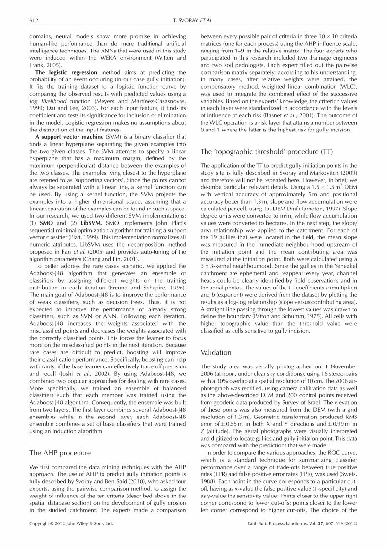
cut-off thus represents a trade-off between sensitivity andspecificity. Ideally, one wants high values of both, so the modelcan well predict both ‘gully’ and ‘non-gully’ points. Usually, alow cut-off gives a higher sensitivity. Conversely, a high cut-off gives a lower false positive rate, at the price of lowersensitivity. In terms of classifier comparison, the best curve isthe one that is leftmost, the ideal one coinciding with they-axis. Thus, the AUC is an accepted performance metric foran ROC curve (Bradley, 1997). The AUC range is 0–1. The areaunder the diagonal is 0.5. This value represents a randomclassifier. On the other hand, a value of 1 represents an optimalclassifier. The diagonal line that appears in Figure 6 indicatesthe curve for random prediction. The various techniques werecompared using the area under ROC parameter.The ROC curves can also guide the choice of an optimal

threshold. One common approach is to choose the thresholdthat will make the resulting classification as close to perfect aspossible. Specifically, we look for the closet point to the upperleft corner (i.e., the perfect classification with true positive = 1and false positive = 0). The distance between a point in thegraph and the perfect point ismeasured using Euclidean distance.Table I describes the optimal thresholds for the various methods.We conclude that in all cases the threshold obtained is relativelyhigh due to the imbalance in the dataset. An alternative way forfinding the optimal threshold is to consider the costs and utilitiesattached to the decision made by the classifier. However,because the values of these costs are usually determinedad-hoc, we did not examine this approach.

Results

The results of this study are ordered in the following manner.First, we compare the predictions of gully initiation points byDM and AHP. We then compare the DM prediction results withthose achieved by the use of TT. Finally, we show the rules thatwere extracted by the DM procedure.

Figure 6. Example of ROC curve: different threshold points aremarked on the upper ROC curve. The lower diagonal line is the ROCcurve for random prediction. FPR refers to false positive error rate andTPR stands for true positive error rate.

Table I. Optimal threshold values according to the closet point to theupper left point (optimal point).

Method Optimal threshold

AdaBoost (J48) 0.918285LibSVM 0.899521SMO 0.947337Logistic 0.836336Multi-layer Perceptron 0.812902


DM versus AHP

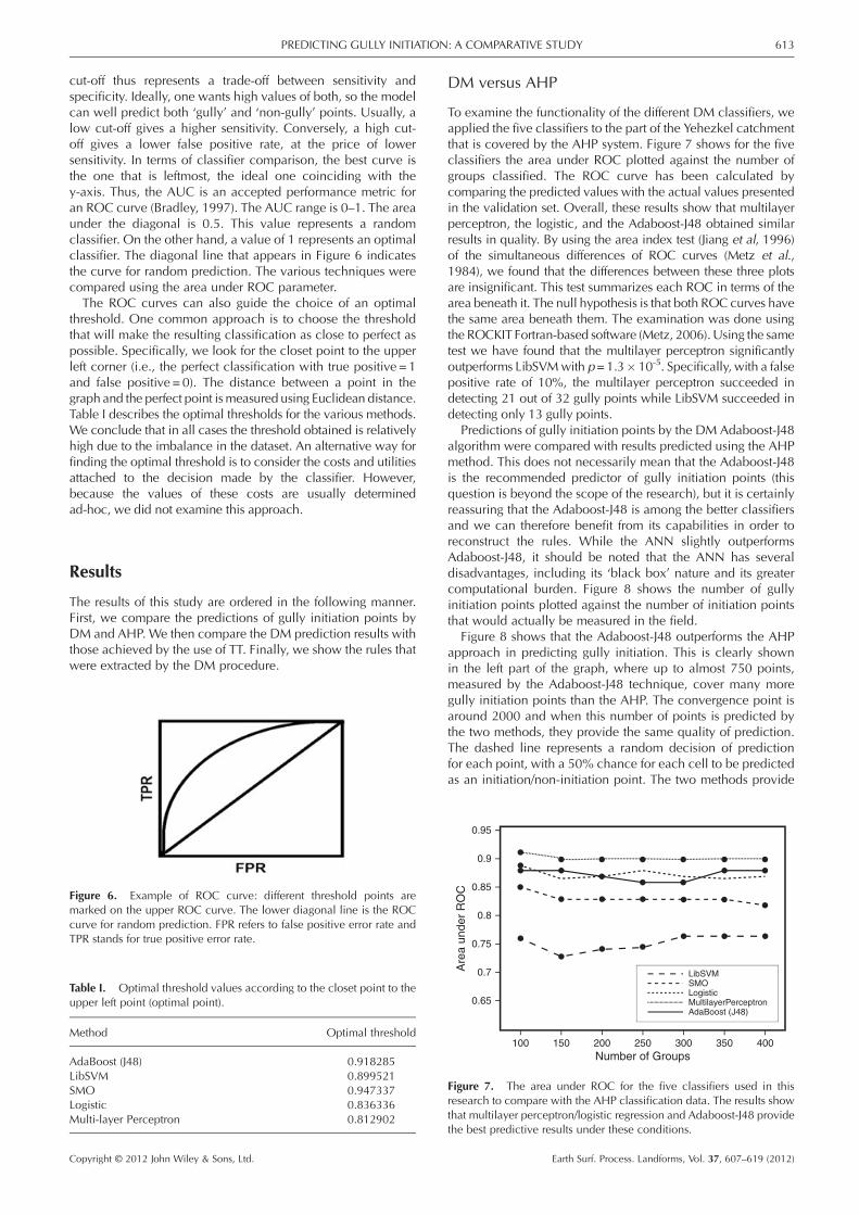
To examine the functionality of the different DM classifiers, weapplied the five classifiers to the part of the Yehezkel catchmentthat is covered by the AHP system. Figure 7 shows for the fiveclassifiers the area under ROC plotted against the number ofgroups classified. The ROC curve has been calculated bycomparing the predicted values with the actual values presentedin the validation set. Overall, these results show that multilayerperceptron, the logistic, and the Adaboost-J48 obtained similarresults in quality. By using the area index test (Jiang et al, 1996)of the simultaneous differences of ROC curves (Metz et al.,1984), we found that the differences between these three plotsare insignificant. This test summarizes each ROC in terms of thearea beneath it. The null hypothesis is that both ROC curves havethe same area beneath them. The examination was done usingthe ROCKIT Fortran-based software (Metz, 2006). Using the sametest we have found that the multilayer perceptron significantlyoutperforms LibSVMwith p=1.3� 10-5. Specifically, with a falsepositive rate of 10%, the multilayer perceptron succeeded indetecting 21 out of 32 gully points while LibSVM succeeded indetecting only 13 gully points.

Predictions of gully initiation points by the DM Adaboost-J48algorithm were compared with results predicted using the AHPmethod. This does not necessarily mean that the Adaboost-J48is the recommended predictor of gully initiation points (thisquestion is beyond the scope of the research), but it is certainlyreassuring that the Adaboost-J48 is among the better classifiersand we can therefore benefit from its capabilities in order toreconstruct the rules. While the ANN slightly outperformsAdaboost-J48, it should be noted that the ANN has severaldisadvantages, including its ‘black box’ nature and its greatercomputational burden. Figure 8 shows the number of gullyinitiation points plotted against the number of initiation pointsthat would actually be measured in the field.

Figure 8 shows that the Adaboost-J48 outperforms the AHPapproach in predicting gully initiation. This is clearly shownin the left part of the graph, where up to almost 750 points,measured by the Adaboost-J48 technique, cover many moregully initiation points than the AHP. The convergence point isaround 2000 and when this number of points is predicted bythe two methods, they provide the same quality of prediction.The dashed line represents a random decision of predictionfor each point, with a 50% chance for each cell to be predictedas an initiation/non-initiation point. The two methods provide

100 150 200 250 300 350 400

0.65

0.7

0.75

0.8

0.85

0.95

0.9

Number of Groups

Are

a un

der

RO

C

LibSVMSMOLogisticMultilayerPerceptronAdaBoost (J48)

igure 7. The area under ROC for the five classifiers used in thissearch to compare with the AHP classification data. The results showat multilayer perceptron/logistic regression and Adaboost-J48 providee best predictive results under these conditions.

Frethth


00

30001000 2000

5

10

15

20

25

35

30

Total number of Points

Gul

ly In

itiat

ion

Poi

nt

RandomAdaBoost (J48)AHP

Figure 8. The number of gully initiation points identified, plottedagainst the percentage of points (cells) searched by both the AHP andthe DM procedures. The results show that the Adaboost-J48 outperformsthe AHP, while convergence occurs towards 2000 points searched. Bothmethods outperform random sampling.

100 150 200 250 300 350 400

0.5

0.52

0.54

0.56

0.58

0.6

0.64

0.62

Number of Groups

Are

a un

der

RO

C

LibSVMSMOLogisticMultilayerPerceptronAdaBoost (J48)

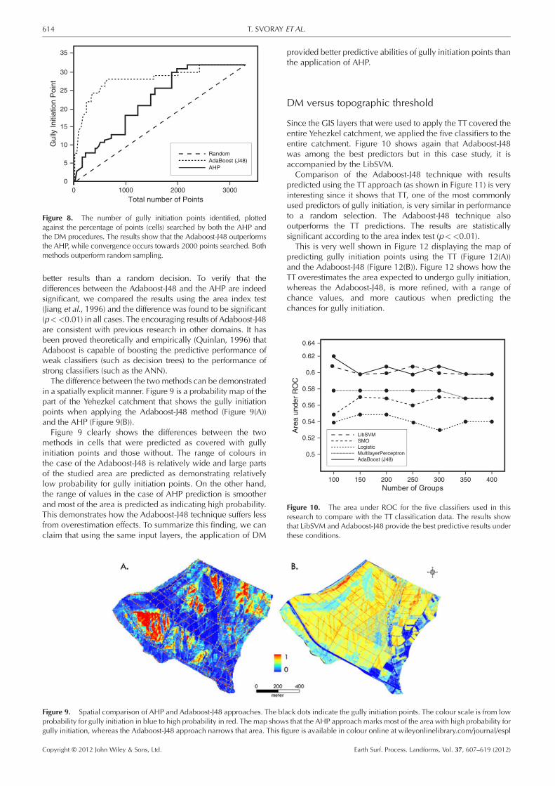
Figure 10. The area under ROC for the five classifiers used in thisresearch to compare with the TT classification data. The results showthat LibSVM and Adaboost-J48 provide the best predictive results underthese conditions.


better results than a random decision. To verify that thedifferences between the Adaboost-J48 and the AHP are indeedsignificant, we compared the results using the area index test(Jiang et al., 1996) and the difference was found to be significant(p<<0.01) in all cases. The encouraging results of Adaboost-J48are consistent with previous research in other domains. It hasbeen proved theoretically and empirically (Quinlan, 1996) thatAdaboost is capable of boosting the predictive performance ofweak classifiers (such as decision trees) to the performance ofstrong classifiers (such as the ANN).The difference between the two methods can be demonstrated

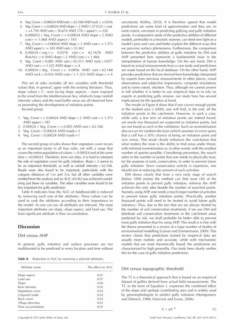
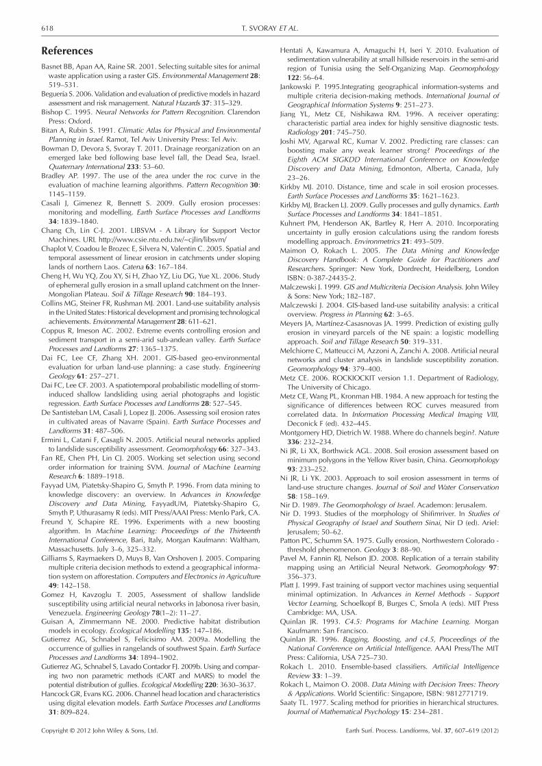
in a spatially explicit manner. Figure 9 is a probability map of thepart of the Yehezkel catchment that shows the gully initiationpoints when applying the Adaboost-J48 method (Figure 9(A))and the AHP (Figure 9(B)).Figure 9 clearly shows the differences between the two

methods in cells that were predicted as covered with gullyinitiation points and those without. The range of colours inthe case of the Adaboost-J48 is relatively wide and large partsof the studied area are predicted as demonstrating relativelylow probability for gully initiation points. On the other hand,the range of values in the case of AHP prediction is smootherand most of the area is predicted as indicating high probability.This demonstrates how the Adaboost-J48 technique suffers lessfrom overestimation effects. To summarize this finding, we canclaim that using the same input layers, the application of DM

Figure 9. Spatial comparison of AHP and Adaboost-J48 approaches. The blprobability for gully initiation in blue to high probability in red. The map showgully initiation, whereas the Adaboost-J48 approach narrows that area. This fi


provided better predictive abilities of gully initiation points thanthe application of AHP.

DM versus topographic threshold

Since the GIS layers that were used to apply the TT covered theentire Yehezkel catchment, we applied the five classifiers to theentire catchment. Figure 10 shows again that Adaboost-J48was among the best predictors but in this case study, it isaccompanied by the LibSVM.

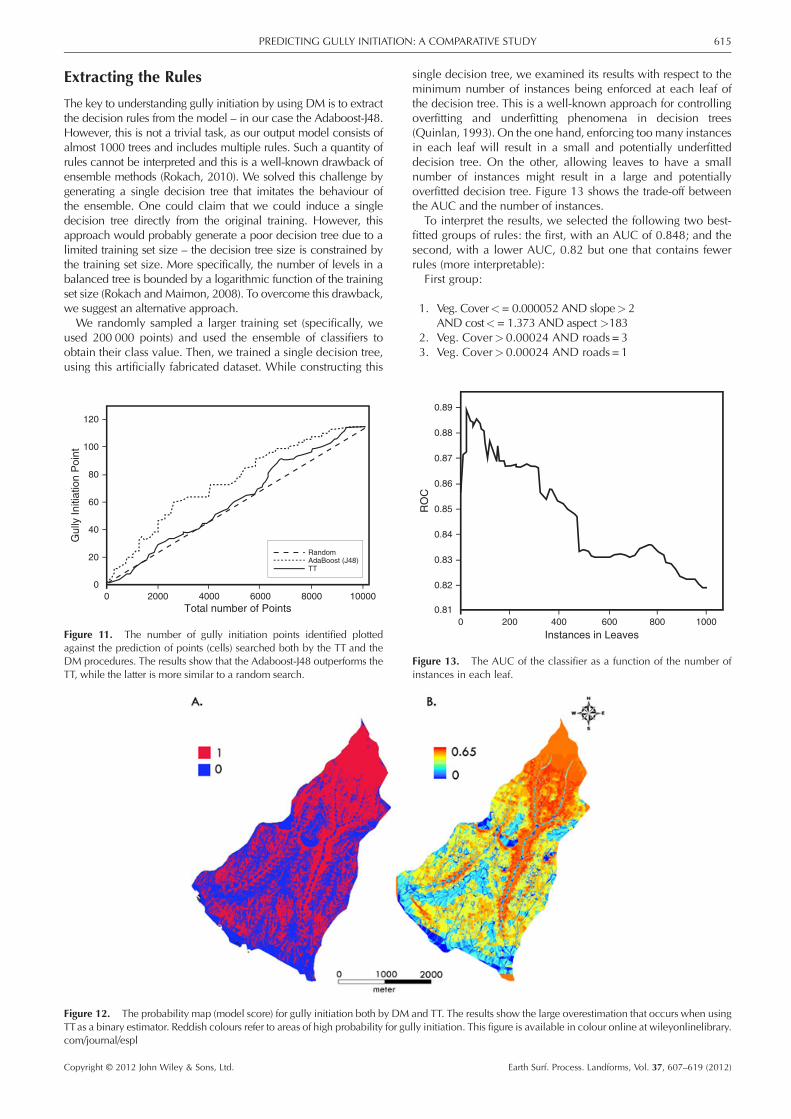
Comparison of the Adaboost-J48 technique with resultspredicted using the TT approach (as shown in Figure 11) is veryinteresting since it shows that TT, one of the most commonlyused predictors of gully initiation, is very similar in performanceto a random selection. The Adaboost-J48 technique alsooutperforms the TT predictions. The results are statisticallysignificant according to the area index test (p<<0.01).

This is very well shown in Figure 12 displaying the map ofpredicting gully initiation points using the TT (Figure 12(A))and the Adaboost-J48 (Figure 12(B)). Figure 12 shows how theTT overestimates the area expected to undergo gully initiation,whereas the Adaboost-J48, is more refined, with a range ofchance values, and more cautious when predicting thechances for gully initiation.

ack dots indicate the gully initiation points. The colour scale is from lows that the AHP approach marks most of the area with high probability forgure is available in colour online at wileyonlinelibrary.com/journal/espl



Extracting the Rules

The key to understanding gully initiation by using DM is to extractthe decision rules from the model – in our case the Adaboost-J48.However, this is not a trivial task, as our output model consists ofalmost 1000 trees and includes multiple rules. Such a quantity ofrules cannot be interpreted and this is a well-known drawback ofensemble methods (Rokach, 2010). We solved this challenge bygenerating a single decision tree that imitates the behaviour ofthe ensemble. One could claim that we could induce a singledecision tree directly from the original training. However, thisapproach would probably generate a poor decision tree due to alimited training set size – the decision tree size is constrained bythe training set size. More specifically, the number of levels in abalanced tree is bounded by a logarithmic function of the trainingset size (Rokach and Maimon, 2008). To overcome this drawback,we suggest an alternative approach.We randomly sampled a larger training set (specifically, we

used 200 000 points) and used the ensemble of classifiers toobtain their class value. Then, we trained a single decision tree,using this artificially fabricated dataset. While constructing this

01000080006000400020000

20

40

60

80

120

100

Total number of Points

Gul

ly In

itiat

ion

Poi

nt

RandomAdaBoost (J48)TT

Figure 11. The number of gully initiation points identified plottedagainst the prediction of points (cells) searched both by the TT and theDM procedures. The results show that the Adaboost-J48 outperforms theTT, while the latter is more similar to a random search.

Figure 12. The probability map (model score) for gully initiation both by DMTTas a binary estimator. Reddish colours refer to areas of high probability for gucom/journal/espl


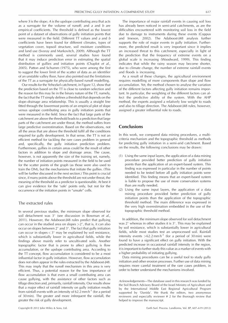
single decision tree, we examined its results with respect to theminimum number of instances being enforced at each leaf ofthe decision tree. This is a well-known approach for controllingoverfitting and underfitting phenomena in decision trees(Quinlan, 1993). On the one hand, enforcing too many instancesin each leaf will result in a small and potentially underfitteddecision tree. On the other, allowing leaves to have a smallnumber of instances might result in a large and potentiallyoverfitted decision tree. Figure 13 shows the trade-off betweenthe AUC and the number of instances.

To interpret the results, we selected the following two best-fitted groups of rules: the first, with an AUC of 0.848; and thesecond, with a lower AUC, 0.82 but one that contains fewerrules (more interpretable):

First group:

1. Veg. Cover<= 0.000052 AND slope> 2AND cost<= 1.373 AND aspect >183

2. Veg. Cover> 0.00024 AND roads = 33. Veg. Cover> 0.00024 AND roads = 1

and TT. The results show the large overestimation that occurs when usinglly initiation. This figure is available in colour online at wileyonlinelibrary.

0.81400 600 800200 10000

0.82

0.83

0.84

0.85

0.86

0.87

0.88

0.89

Instances in Leaves

RO

C

Figure 13. The AUC of the classifier as a function of the number ofinstances in each leaf.



4. Veg.Cover>0.00024ANDrain>62.168ANDrock<=0.0165. Veg. Cover<=0.00024AND slope> 2AND1.373123< cost

<=1.759 AND rain> 50.674 AND 178< aspect<= 2266. 0.000052<Veg. Cover<= 0.00024 AND slope>2 AND

cost<= 1.068 AND aspect>1837. Veg. Cover<= 0.00024 AND slope>2 AND cost<= 1.373

AND aspect<= 183 AND rain> 53.3628. 0.00024< veg<= 0.0276 rain<= 62.1678 AND

flowAcc> 4 AND slope>2 AND cost<= 1.4669. Veg. Cover> 0.085 AND rain> 65.313 AND rock> 0.077

AND cost<= 1.323 AND slope<= 410. 0.00024<Veg. Cover<= 0.0856 AND rain> 62.168

AND rock> 0.016 AND cost<= 1.323 AND slope<= 4

This set of rules includes all ten variables with thresholdvalues that, in general, agree with the existing literature. Thus,slope values> 2�, west facing slope aspects – more exposedto the wind from the Mediterranean Sea, relatively large rainfallintensity values and the road buffer areas are all observed hereas promoting the development of initiation points.Second group:

1. Veg. Cover<= 0.00024 AND slope> 2 AND cost<= 1.373AND aspect> 183

2. 0.00024<Veg. Cover<= 0.005 AND rain>62.1683. Veg. Cover> 0.00024 AND roads = 34. Veg. Cover> 0.00024 AND roads = 1

The second group of rules shows that vegetation cover recursas an important factor in all four rules, yet with a range thatcovers the entire population of values:> 0.00024 and at the sametime<=0.00024. Therefore, from our data, it is hard to interpretthe role of vegetation cover for gully initiation. Slope>2 seems tobe an important threshold, as well as rainfall intensity> 62.168.Roads were also found to be important, particularly with thecategory distances of 1m and 3m, but all other variables wereomitted from the analysis and an AUC of 0.82was achieved consid-ering just these six variables. The other variables were found to beless important for gully prediction.Table II indicates how the AUC of AdaBoost-J48 is reduced

by removing each one of the attributes. These values can beused to rank the attributes according to their importance tothe model. As one can see all attributes are relevant. The mostimportant attributes are slope, slope aspect, and land use. Theleast significant attribute is flow accumulation.

Discussion

DM versus AHP

In general, gully initiation and surface processes are toomultifaceted to be predicted in every location and time without

Table II. Reduction in AUC by removing a selected attributes.

Attribute name The effect on AUC

Slope aspect 0.07Land use 0.07Slope 0.06Rain intensity 0.03Vegetation cover 0.03Unpaved roads 0.02Rock cover 0.02Tillage direction 0.01Flow accumulation 0.01


uncertainty (Kirkby, 2010). It is therefore agreed that modelpredictions are some kind of approximation and they are, tosome extent, uncertain in predicting gullying and gully initiationpoints. A comparative study of the predictive abilities of differentmodels, preferably in a heuristic manner, can shed new light on amodel’s pros and cons and better explain the different ways thatwe perceive surface phenomena. Furthermore, the comparisonbetween the predictive abilities of gully initiation by DM andAHP presented here represents a fundamental issue in theinterpretation of human knowledge. On the one hand, DM isbased on actual measurements from a case study and predictionsare made based on the local database. On the other hand, AHPprovides predictions that are derived from knowledge interpretedby experts from previous measurements in other places, visualobservations and subjective impressions, computer simulationsand to some extent, intuition. Thus, although we cannot answerin full whether it is better to use empirical data or to rely onexperts in predicting gully erosion, our study here has severalimplications for the question at hand.

The results in Figure 8 show that if one covers enough pointsin the studied area (~2000), one will find, in the end, all theinitiation points in the catchment. However, in such a case,while only a few tens of initiation points are indeed found,yet nearly two thousand are suspected as initiation points, butare not found as such in the validation. Such an overestimationalso occurs for random decision (which assumes in every querythat a cell has a 50% chance of being an initiation point andvice versa). This result clearly enhances the conclusion thatwhat matters the most is the ability to find areas under threat,with minimal overestimation or, in other words, with the smallestnumber of queries possible. Considering prevention, the searchrefers to the number of points that one needs to physically treat,for the purpose of early conservation, in order to prevent futuregully initiation. Since conservation activity is expensive, oneshould aim at reducing the amount of such activities.

DM shows clearly that from a very early stage of search(below 1000 points) the method can find most (30) of theinitiation points to prevent gully initiation, whereas the AHPachieves this only after double the number of searched points.Namely, using AHP, one needs amuch larger number of activitiesto prevent future gully initiation points. (Practically, anotherthousand points will need to be treated to avoid future gullyinitiation.) Thus, due to the fact that we are always limited bythe number of soil conservation treatments, if we use DM anddistribute soil conservation treatments in the catchment areaspredicted by risk, we shall probably be better able to preventmore gully initiation than by using AHP. This result is in line withthe theory presented in a review of a large number of studies ofenvironmental modelling (Guisan and Zimmermann, 2000). Thisreview claims that predictions trained by empirical data areusually more realistic and accurate, while with mechanisticmodels that are more theoretically based, the predictions arecharacterized by high generality. Our study here clearly verifiesthis for the case of gully initiation predictions.

DM versus topographic threshold

The TT is a theoretical approach that is based on an empiricaldataset of gullies derived from actual field measurements. TheTT, in the form of Equation 1, expresses the combined effectof the slope and upslope contributing area and is widely usedby geomorphologists to predict gully initiation (Montgomeryand Dietrich, 1988; Hancock and Evans, 2006).

S ¼ aA�b (1)



where S is the slope; A is the upslope contributing area that actsas a surrogate for the volume of runoff; and a and b areempirical coefficients. The threshold is defined as the lowestpoint of a dataset of observations of gully initiation points thatwere measured in the field. Different TT values and a and bcoefficients have been found for different climates, types ofvegetation cover, topsoil structure, soil moisture conditionsand land use (Svoray and Markovitch, 2009). Although the TTmethod is commonly used, several studies have foundthat it may induce prediction error in estimating the spatialdistribution of gullies and initiation points (Chaplot et al.,2005). Patton and Schumm (1975), who were among the firstto suggest the lower limit of the scatter of data as an identifierof an unstable valley floor, have also pointed out the limitationsof the TT as a surrogate for physically-based runoff modelling.Our results for the Yehezkel catchment, in Figure 12, show that

the prediction based on the TT is close to random selection andthe reason for this may lie in the binary nature of the TT, namely,the fact that the TTsimply defines a threshold that depends on theslope–drainage area relationship. This is usually a straight linefitted through the lowermost points of an empirical plot of slopeversus upslope contributing area in gully initiation points thatwere measured in the field. Since the fact that large parts of thecatchment are above the threshold leads to a prediction that largeparts of the catchment are under threat, the method suffers fromlarge predictive overestimation. Based on the observations, notall the areas that are above the threshold fulfil all the conditionsrequired for gully development. In that sense, the TT is not anefficient method for tackling the rare cases problem in generaland, specifically, the gully initiation prediction problem.Furthermore, gullies in certain areas could be the result of otherfactors in addition to slope and drainage areas. The cause,however, is not apparently the size of the training set, namely,the number of initiation points measured in the field to be usedfor the scatter points of the graph (as those were also used totrain the DM), but the mechanisms that initiate the gullies. (Thiswill be further discussed in the next section.) This point is crucialsince, if many points above the threshold are not under threat, themeaning of the threshold as a predictor is questionable. At best itcan give evidence for the ‘safe’ points only, but not for theoccurrence of the initiation points in “unsafe” cells.

The extracted rules

In several previous studies, the minimum slope observed forsoil detachment was 3� (see discussion in Bowman et al.,2011). However, the Adaboost-J48 rules predict that gullyingcan occur in the studied area on slopes >2�, that is, it can alsooccur on slopes between 2� and 3�. The fact that gully initiationcan occur in slopes< 3� may be explained by soil resistance,which is substantially lower in agricultural fields, while thefindings above mainly refer to uncultivated soils. Anothertopographic factor that is prone to affect gullying is flowaccumulation, or the upslope contributing area. According tothe TT concept, flow accumulation is considered to be a mostinfluential factor in gully initiation. However, flow accumulationdoes not often appear in the rules extracted by the Adaboost-J48.This may imply that the runoff mechanism in this area is veryefficient. Thus, a potential reason for the low importance offlow accumulation is that even a small contributing area cancause gullying, with the assistance of other factors such astillage direction and, primarily, rainfall intensity. Our results showthat a major effect of rainfall intensity on gully initiation resultsfrom rainfall events with an intensity of 62.2mmh-1 (for a periodof 30min). The greater and more infrequent the rainfall, thegreater the risk of gully development.


The importance of major rainfall events in causing soil losshas already been noticed in semi-arid catchments, as are thedifficulties encountered with monitoring soil loss in the fielddue to damage to instruments during these events (Coppusand Imeson, 2002). The Adaboost-J48 analysis furthersupports the role of major events in gully initiation. Further-more, the predicted result is very important since it impliesan increased threat to this catchment, especially in light ofthe prediction that the frequency of extreme events on aglobal scale is increasing (Woodward, 1999). This findingindicates that while the rainy season may become shorter,due to climate change, the number of extreme rainfall eventsand floods is increasing.

As a result of these changes, the agricultural environmentrequires modelling of more components than slope and flowaccumulation. Yet, the method chosen to analyse the variationof the different factors affecting gully initiation remains impor-tant. In particular, the weighting of the different factors can af-fect the predictive ability of the system. With the AHPmethod, the experts assigned a relatively low weight to roadsand also to tillage direction. The Adaboost-J48 rules, however,assigned a greater influential role to roads.

Conclusions

In this work, we compared data mining procedures, a multi-criteria mechanism and the topographic threshold as methodsfor predicting gully initiation in a semi-arid catchment. Basedon the results, the following conclusions may be drawn:

(1) Using the same input layers, the application of a data miningprocedure provided better prediction of gully initiationpoints than the application of an expert-based system. Thisfinding was expressed in particular in the number of pointsneeded to be tested before all gully initiation points wereidentified. This finding means that an expert-based systemis liable to propose the use of more conservation systemsthan are really needed.

(2) Using the same input layers, the application of a datamining procedure provided better prediction of gullyinitiation points than the application of the topographicthreshold method. The main difference was expressed inthe very high overestimation embedded in the use of thetopographic threshold method.

In addition, the minimum slope observed for soil detachmentwas 2� whereas in other studies it is 3�. This may be explainedby soil resistance, which is substantially lower in agriculturalfields, while most studies test an unprocessed soil. Rainfallintensity events >62.2mmh-1 (for a period of 30min) werefound to have a significant effect on gully initiation. With thepredicted increase in occasional rainfall intensity in the region,it is important to further study this value as amarker of eventswitha higher probability of initiating gullying.

Data mining procedures can be a useful tool to study gullyinitiation and other erosion processes. Further use of data miningrequires more careful treatment of the rare cases problem, inorder to better understand the mechanisms involved.

Acknowledgements—The database used in this research was funded bythe Soil Branch Advisory Board of the Israel Ministry of Agriculture andby the International Middle East Regional Agricultural Programsupported by ‘Danida’. We thank the editors, two anonymousreviewers and especially reviewer # 2 for the thorough review thathelped to improve the manuscript.



ReferencesBasnet BB, Apan AA, Raine SR. 2001. Selecting suitable sites for animalwaste application using a raster GIS. Environmental Management 28:519–531.

Beguería S. 2006. Validation and evaluation of predictivemodels in hazardassessment and risk management. Natural Hazards 37: 315–329.

Bishop C. 1995. Neural Networks for Pattern Recognition. ClarendonPress: Oxford.

Bitan A, Rubin S. 1991. Climatic Atlas for Physical and EnvironmentalPlanning in Israel. Ramot, Tel Aviv University Press: Tel Aviv.

Bowman D, Devora S, Svoray T. 2011. Drainage reorganization on anemerged lake bed following base level fall, the Dead Sea, Israel.Quaternary International 233: 53–60.

Bradley AP. 1997. The use of the area under the roc curve in theevaluation of machine learning algorithms. Pattern Recognition 30:1145–1159.

Casali J, Gimenez R, Bennett S. 2009. Gully erosion processes:monitoring and modelling. Earth Surface Processes and Landforms34: 1839–1840.

Chang Ch, Lin C-J. 2001. LIBSVM - A Library for Support VectorMachines. URL http://www.csie.ntu.edu.tw/~cjlin/libsvm/

Chaplot V, Coadou le Brozec E, Silvera N, Valentin C. 2005. Spatial andtemporal assessment of linear erosion in catchments under slopinglands of northern Laos. Catena 63: 167–184.

Cheng H, Wu YQ, Zou XY, Si H, Zhao YZ, Liu DG, Yue XL. 2006. Studyof ephemeral gully erosion in a small upland catchment on the Inner-Mongolian Plateau. Soil & Tillage Research 90: 184–193.

Collins MG, Steiner FR, Rushman MJ. 2001. Land-use suitability analysisin theUnited States: Historical development and promising technologicalachievements. Environmental Management 28: 611–621.

Coppus R, Imeson AC. 2002. Extreme events controlling erosion andsediment transport in a semi-arid sub-andean valley. Earth SurfaceProcesses and Landforms 27: 1365–1375.

Dai FC, Lee CF, Zhang XH. 2001. GIS-based geo-environmentalevaluation for urban land-use planning: a case study. EngineeringGeology 61: 257–271.

Dai FC, Lee CF. 2003. A spatiotemporal probabilistic modelling of storm-induced shallow landsliding using aerial photographs and logisticregression. Earth Surface Processes and Landforms 28: 527–545.

De Santisteban LM, Casali J, Lopez JJ. 2006. Assessing soil erosion ratesin cultivated areas of Navarre (Spain). Earth Surface Processes andLandforms 31: 487–506.

Ermini L, Catani F, Casagli N. 2005. Artificial neural networks appliedto landslide susceptibility assessment. Geomorphology 66: 327–343.

Fan RE, Chen PH, Lin CJ. 2005. Working set selection using secondorder information for training SVM. Journal of Machine LearningResearch 6: 1889–1918.

Fayyad UM, Piatetsky-Shapiro G, Smyth P. 1996. From data mining toknowledge discovery: an overview. In Advances in KnowledgeDiscovery and Data Mining, FayyadUM, Piatetsky-Shapiro G,Smyth P, Uthurasamy R (eds). MIT Press/AAAI Press: Menlo Park, CA.

Freund Y, Schapire RE. 1996. Experiments with a new boostingalgorithm. In Machine Learning: Proceedings of the ThirteenthInternational Conference, Bari, Italy, Morgan Kaufmann: Waltham,Massachusetts. July 3–6, 325–332.

Gilliams S, Raymaekers D, Muys B, Van Orshoven J. 2005. Comparingmultiple criteria decision methods to extend a geographical informa-tion system on afforestation. Computers and Electronics in Agriculture49: 142–158.

Gomez H, Kavzoglu T. 2005, Assessment of shallow landslidesusceptibility using artificial neural networks in Jabonosa river basin,Venezuela. Engineering Geology 78(1–2): 11–27.

Guisan A, Zimmermann NE. 2000. Predictive habitat distributionmodels in ecology. Ecological Modelling 135: 147–186.

Gutierrez AG, Schnabel S, Felicisimo AM. 2009a. Modelling theoccurrence of gullies in rangelands of southwest Spain. Earth SurfaceProcesses and Landforms 34: 1894–1902.

Gutierrez AG, Schnabel S, Lavado Contador FJ. 2009b. Using and compar-ing two non parametric methods (CART and MARS) to model thepotential distribution of gullies. Ecological Modelling 220: 3630–3637.

HancockGR, Evans KG. 2006. Channel head location and characteristicsusing digital elevation models. Earth Surface Processes and Landforms31: 809–824.


Hentati A, Kawamura A, Amaguchi H, Iseri Y. 2010. Evaluation ofsedimentation vulnerability at small hillside reservoirs in the semi-aridregion of Tunisia using the Self-Organizing Map. Geomorphology122: 56–64.

Jankowski P. 1995.Integrating geographical information-systems andmultiple criteria decision-making methods. International Journal ofGeographical Information Systems 9: 251–273.

Jiang YL, Metz CE, Nishikawa RM. 1996. A receiver operating:characteristic partial area index for highly sensitive diagnostic tests.Radiology 201: 745–750.

Joshi MV, Agarwal RC, Kumar V. 2002. Predicting rare classes: canboosting make any weak learner strong? Proceedings of theEighth ACM SIGKDD International Conference on KnowledgeDiscovery and Data Mining, Edmonton, Alberta, Canada, July23–26.

Kirkby MJ. 2010. Distance, time and scale in soil erosion processes.Earth Surface Processes and Landforms 35: 1621–1623.

Kirkby MJ, Bracken LJ. 2009. Gully processes and gully dynamics. EarthSurface Processes and Landforms 34: 1841–1851.

Kuhnert PM, Henderson AK, Bartley R, Herr A. 2010. Incorporatinguncertainty in gully erosion calculations using the random forestsmodelling approach. Environmetrics 21: 493–509.

Maimon O, Rokach L. 2005. The Data Mining and KnowledgeDiscovery Handbook: A Complete Guide for Practitioners andResearchers. Springer: New York, Dordrecht, Heidelberg, LondonISBN: 0-387-24435-2.

Malczewski J. 1999. GIS and Multicriteria Decision Analysis. John Wiley& Sons: New York; 182–187.

Malczewski J. 2004. GIS-based land-use suitability analysis: a criticaloverview. Progress in Planning 62: 3–65.

Meyers JA, Martínez-Casasnovas JA. 1999. Prediction of existing gullyerosion in vineyard parcels of the NE spain: a logistic modellingapproach. Soil and Tillage Research 50: 319–331.

Melchiorre C, Matteucci M, Azzoni A, Zanchi A. 2008. Artificial neuralnetworks and cluster analysis in landslide susceptibility zonation.Geomorphology 94: 379–400.

Metz CE. 2006. ROCKIOCKIT version 1.1. Department of Radiology,The University of Chicago.

Metz CE, Wang PL, Kronman HB. 1984. A new approach for testing thesignificance of differences between ROC curves measured fromcorrelated data. In Information Processing Medical Imaging VIII,Deconick F (ed). 432–445.

Montgomery HD, Dietrich W. 1988. Where do channels begin?.Nature336: 232–234.

Ni JR, Li XX, Borthwick AGL. 2008. Soil erosion assessment based onminimum polygons in the Yellow River basin, China. Geomorphology93: 233–252.

Ni JR, Li YK. 2003. Approach to soil erosion assessment in terms ofland-use structure changes. Journal of Soil and Water Conservation58: 158–169.

Nir D. 1989. The Geomorphology of Israel. Academon: Jerusalem.Nir D. 1993. Studies of the morphology of Shifimriver. In Studies ofPhysical Geography of Israel and Southern Sinai, Nir D (ed). Ariel:Jerusalem; 50–62.

Patton PC, Schumm SA. 1975. Gully erosion, Northwestern Colorado -threshold phenomenon. Geology 3: 88–90.

Pavel M, Fannin RJ, Nelson JD. 2008. Replication of a terrain stabilitymapping using an Artificial Neural Network. Geomorphology 97:356–373.

Platt J. 1999. Fast training of support vector machines using sequentialminimal optimization. In Advances in Kernel Methods - SupportVector Learning, Schoelkopf B, Burges C, Smola A (eds). MIT PressCambridge: MA, USA.

Quinlan JR. 1993. C4.5: Programs for Machine Learning. MorganKaufmann: San Francisco.

Quinlan JR. 1996. Bagging, Boosting, and c4.5, Proceedings of theNational Conference on Artificial Intelligence. AAAI Press/The MITPress: California, USA 725–730.

Rokach L. 2010. Ensemble-based classifiers. Artificial IntelligenceReview 33: 1–39.

Rokach L, Maimon O. 2008. Data Mining with Decision Trees: Theory& Applications. World Scientific: Singapore, ISBN: 9812771719.

Saaty TL. 1977. Scaling method for priorities in hierarchical structures.Journal of Mathematical Psychology 15: 234–281.


http://www.csie.ntu.edu.tw/~cjlin/libsvm/


Saito, H. Nakayama, D, Matsuyama H. 2009. Comparison of landslidesusceptibility based on a decision-tree model and actual landslide occur-rence: the Akaishi Mountains, Japan. Geomorphology 109: 108–121.

Shu C, Burn DH. 2004. Artificial neural network ensembles and theirapplication in pooled flood frequency analysis. Water ResourcesResearch 40: 1–10.

SvorayT, Ben-Said S. 2010. Soil loss,water ponding and sediment depositionvariations as a consequence of rainfall intensity and land use: a multi-criteria analysis. Earth Surface Processes and Landforms 35: 202–216.

Svoray T, Markovitch H. 2009. Catchment scale analysis of the effect oftopography, tillage direction and unpaved roads on ephemeral gullyincision. Earth Surface Processes and Landforms 34: 1970–1984.

Swets JA. 1988. Measuring the accuracy of diagnostic systems. Science240: 1285–1293.

Tarboton DG, Bras RL, Rodriguez-Iturbe I. 1989. The analysis ofriver basins and channel networks using digital terrain data. TR 326,Department of Civil and Environmental Engineering, MassachusettsInstitute of Technology, Boston.


Tarboton DG. 1997. A new method for the determination of flowdirections and upslope areas in grid digital elevation models. WaterResources Research 33: 309–319.

Trimble SW, Crosson P. 2000. Land use - US soil erosion rates - mythand reality. Science 289: 248–250.

Van Rompaey A, Bazzoffi P, Dostal T, VerstraetenG, JordanG, Lenhart T,Govers G, Montanarella L. 2003. Modeling off-farm consequences ofsoil erosion in various landscapes in Europe with a spatiallydistributed approach. Proceedings of the OECD Expert Meeting on SoilErosion and Soil Biodiversity Indicators, 25–28 March, Rome, Italy.

Weiss GM. 2010. Mining with rare cases. In The Data Mining andKnowledge Discovery Handbook, Rokach L, Maimon O (eds).Springer: New York/Dordrecht: Heidelberg, London; 765–777, ISBN:0-387-24435-2.

Witten IH, Frank E. 2005. Data Mining: Practical Machine LearningTools and Techniques. Morgan Kaufmann: Waltham, Massachusetts.

Woodward DE. 1999. Method to predict cropland ephemeral gullyerosion. Catena 37: 393–399.


Documents

Predicting gully initiation: comparing data mining ... et al... · techniques, analytical hierarchy processes and the ... which is substantially lower in agricultura l fields, while