Rev. sci. tech. Off. int. Epiz., 2008, 27 (2), 319-330

Predicted climate changes for the years to comeand implications for disease impact studies

D.A. Stone (1, 2)

(1) Atmospheric, Oceanic and Planetary Physics, Department of Physics, University of Oxford, Clarendon Laboratory, Parks Road, Oxford OX1 3PU, United Kingdom. E-mail: stoned@atm.ox.ac.uk(2) Tyndall Centre for Climate Change Research, United Kingdom

SummaryThe paper presents a review of the current ability of the climate modellingcommunity to produce predictions of future climate change. Predictions for thenext few decades are reasonably robust, whereas predictions for later timeperiods depend on uncertainties in climate model structure and on the unknownfuture course of greenhouse gas emissions. Some regional features arenoticeable; however, meaningful interpretation of these can only presently bemade at spatial scales that are considerably larger than those required formaking sound estimates of the effects of future climate change on animal health.The implication is that current climate change predictions should be consideredindicative rather than accurate.

KeywordsClimate – Climate change – Modelling – Prediction – Weather.

Predicting 21st Century weatherWhen someone first starts thinking about the climate, theirfirst question is usually ‘What is the difference betweenweather and climate?’ The answer is often considered quitebasic: the climate is the average weather (at a given placeand time of day and year). Thus, while the weather canchange from minute to minute, the climate is constantfrom year to year. But this question is in fact much moreperceptive: how can we be predicting climate change whenthe climate is constant?

Edward Lorenz, a central figure in the development ofnumerical weather prediction, said instead that ‘climate iswhat you expect, weather is what you get’ (11, quotingRobert Heinlein, in turn probably quoting Mark Twain).The climate is, then, all of the states of weather that arepossible subject to certain constraints external to theclimate system, i.e. for which there are no meaningfulfeedbacks from the weather. Some of these are changing, asdescribed in the previous paper in this issue (Delecluse

[5]). So as long as we know how these factors will changeand have a ‘perfect’ model of the climate system, we canthen predict future climate exactly, at least in theory.

But of course that climate prediction will never beobserved. What will actually occur is not the distributionof all possible meteorological states given the externalconstraints, but a single realisation: the weather. Thisrealisation will depend not just on the external forcingsdescribed by Delecluse (5), but also on what the weather istoday, because it takes time for heat, air, and water to bemoved about. It matters whether the proverbial Brazilianbutterfly has flapped its wings. Thus, as Lorenz said, whilewe can expect a certain climate, in the end we will get, andthus observe, the weather.

Such distinctions may seem trivial, but they end up beingvital in interpreting predictions of future climate. We donot have a perfect model of the climate system, so all of ourpredictions are inherently uncertain, with the sources andimportance of that uncertainty depending on the relationbetween weather and climate. This paper, a guide to our

expectation of future climate change, must be interpretedin this context. With this in mind, the article begins with adescription of how predictions of future climate arecurrently made and then continues with a discussion ofpredictions of future global climate over shorter timescales(the 2020s) and longer timescales (the 2090s). The paperthen examines predictions at a region level and ends with a discussion of implications for animal disease impact studies.

Methods of predicting future climateContinuation of past trends

Predicting future climate, like any other prediction,requires the use of a model. Under a number ofassumptions, a simple extrapolation of a linear trend fit to recent weather may provide a sufficiently accurateprediction. These assumptions may not always be reasonable, however. For instance, the global warmingover the past century has been driven mainly by a rise inatmospheric concentrations of greenhouse gases, but it hasalso been moderated by scattering of sunlight back to space by a rise in sulphate aerosol amounts originatingfrom human activities (6). The balance is expected tochange in the future though, with greenhouse gasconcentrations continuing to rise but sulphate aerosolamounts being more stable due to smog control measures(17), so a simple linear trend extrapolation may beexpected to underestimate future warming. Consequently,the climate community depends primarily on process-based models of the climate system, explicitly calculatingchanges in physical (and increasingly chemical andvegetative) processes through time.

Simple physical models

Physical climate models can take many forms. Thesimplest physical models represent a zero-dimensionalsystem with a simple delayed response to an externalforcing and can even be calculated analytically for somespecial cases. Because of their simple structure, suchmodels can be statistically tuned against historicalobservations, allowing objective probabilistic estimates offuture climate change under a given scenario of externalforcings (22). Such models are generally restricted tosurface temperature, which responds more directly to external radiative forcings, and on global scales, wherenonlinearities in feedbacks may be expected to be lessimportant. Simple physical models are useful fordiagnosing the effects of uncertainties in future emissions,in physical parametrisations (simple empiricalapproximations), and in changes on millennial timescales,

problems which are unfeasible with more complex modelsusing current computers (15). Notably, climatologists takea similarity of predictions across models of varyingcomplexity as an indication of robustness.

General circulation models

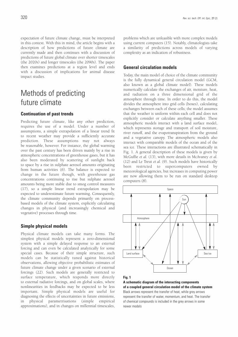
Today, the main model of choice of the climate communityis the fully dynamical general circulation model (GCM,also known as a global climate model). These modelsnumerically calculate the exchanges of air, moisture, heat,and radiation on a three dimensional grid of theatmosphere through time. In order to do this, the modeldivides the atmosphere into grid cells (boxes), calculatingexchanges between each of these cells; the model assumesthat the weather is uniform within each cell and does notexplicitly consider or calculate anything smaller. Theseatmospheric models interact with a land surface model,which represents storage and transport of soil moisture,river runoff, and the evapotranspiration from the groundand a vegetative canopy. The atmospheric models alsointeract with comparable models of the ocean and of thesea ice. These interactions are illustrated schematically inFig. 1. A general description of these models is given byMcGuffie et al. (13), with more details in McAvaney et al.(12) and Le Treut et al. (9). Such models have historicallybeen restricted to supercomputers owned bymeteorological agencies, but increases in computing powerare now allowing them to be run on standard desktopcomputers (8).

Rev. sci. tech. Off. int. Epiz., 27 (2)320

Space

Atmosphere

Land surface Sea ice

Ocean

Sun

Fig. 1A schematic diagram of the interacting components of a coupled general circulation model of the climate systemBlack arrows represent the transfer of heat, while grey arrowsrepresent the transfer of water, momentum, and heat. The transfer of chemical compounds is included in the grey arrows in some newer models

In principle, GCMs fully encapsulate our knowledge of theclimate system. In practice, however, certain shortcutshave to be taken. Most obviously, computing powercurrently restricts the horizontal spatial resolution (the sizeof each grid cell) of the atmospheric component to about200 km (2° latitude/longitude), and the temporalresolution to about 15 minutes, i.e. the model calculateshow the weather would change over 15-minute-long steps,and assumes that the weather does not change over smallertime intervals. A consequence of this is that processeswhich operate at smaller scales, such as mixing of differentair masses, must be represented by simple empiricalapproximations (usually termed parametrisations). Thus,the models do not actually calculate the evolution ofindividual clouds, but rather represent their collectiveproperties at the 200 km scale as a function of othervariables such as humidity. Consequently, differences infuture predictions of global climate change by differentGCMs often come down to how the clouds respond toincreasing greenhouse gas concentrations, and thusdifferences in the representation of clouds in the differentmodels (20). The oceanic components of the models canhave the same horizontal resolution as their atmosphericcounterparts but are often run with half that resolution(~100 km).

An important misconception is that a GCM with ahorizontal resolution of 200 km produces predictions atthat resolution. While technically true, the output is reallyonly meaningful on much larger scales, about 5 to 10 timesas large. Because of the complicated nature of fluid flows,the weather over a given area depends on what ishappening at spatial scales both larger and smaller than thearea being considered. For instance, the weather oversouthern England depends both on the large-scale patternof low and high pressure systems and on the small-scaledetails of local topography and cloud structure.Consequently, the variability in weather over a GCM gridcell relies strongly on the empirical parametrisations whichare representing the smaller-scale processes. Theseparametrisations are only heuristic approximations so weexpect the model to perform badly at this scale. However,at several times the model resolution we may begin tosuppose that the GCM is truly modelling the relevantsmaller processes, although whether this supposition isreasonable is the big unknown in climate modelling. Themain message, then, is that current GCM output should beinterpreted only at scales greater than about 1,000 km.

Regional climate models

The coarseness of the spatial resolution of GCMs is clearlya major problem for determining the effect of climatechange on a disease that is influenced by a much morelocal environment. There are two main approaches to

dealing with this issue (10). One is to actually increase theresolution but only over a smaller region of interest. This isusually done by feeding the meteorological states from aGCM simulation along the borders of the smaller regioninto a regional version of a GCM, termed a nested regionalclimate model or RCM (2, 14). Current RCMs typically runat resolutions of about 30 km. Because RCMs are physically modelling the relevant processes, they areallowing for local responses to external forcings that are not possible to consider with coarser global models.The big assumption in RCMs is, however, that anythinghappening at sub-grid scales outside of the region is notimportant for the weather within the region. This may notnecessarily be the case; for instance, both thunderstormsand waves along the oceanic thermocline in the tropicalPacific, through their role in producing so-called El Niñoand La Niña events, can affect weather throughout thetropics and the globe in general. The technical details ofhow to feed GCM data into a higher resolution RCM arealso uncertain.

Empirical downscaling

The other approach for getting around the resolution limitis empirical downscaling, also termed statisticaldownscaling. This uses relationships noted in the observedrecord between some large-scale meteorological quantityand a more local variable (25). For a simple example,rainfall over southern areas of England is highly anti-correlated with surface air pressure over a broad areanorthwest of the United Kingdom. Because this statisticalrelationship is observed and site-specific, it can easilyperform better than the generic parametrisation thatrepresents rainfall in the GCM. Thus, it may even be amore appropriate measure of rainfall in the GCM thanrainfall itself, for this example at least. The inference, then,is that this relationship will hold in a future climate.Empirical downscaling has the advantage of simplicity andof effectively being able to resolve the tiniest of spatialscales. In fact, the target variable can just as easily be non-meteorological and in effect all current climate-diseasemodels downscale already in the conversion ofmeteorological quantities into epidemiological variables.However, empirical downscaling relies absolutely on theavailability of adequate and appropriate historicalobservational records. While this is a requirement of anyapplication of climate model data, the restriction is muchmore specific with empirical downscaling. Moreover, itimplicitly assumes that the relationship between the twoscales is independent of the external forcing, which inmany cases may not be realistic. This issue becomesparticularly acute if future states move outside of thedomain of the states observed in the historical record. Forinstance, the drier soil over continental areas resultingfrom increased evaporation may change the behaviour ofheatwaves in a warmer world (18).

Rev. sci. tech. Off. int. Epiz., 27 (2) 321

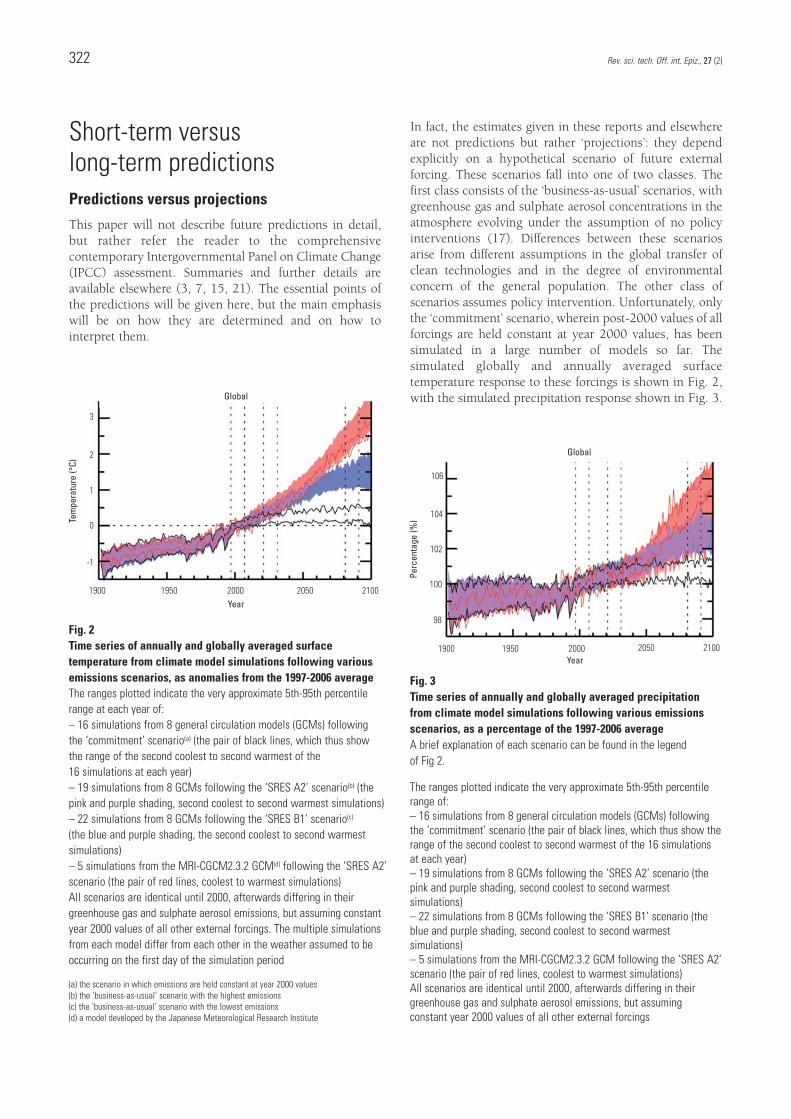
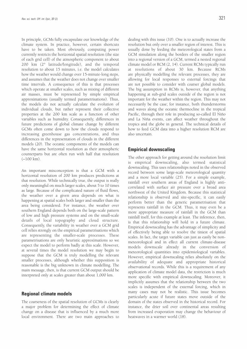
Fig. 3Time series of annually and globally averaged precipitationfrom climate model simulations following various emissionsscenarios, as a percentage of the 1997-2006 averageA brief explanation of each scenario can be found in the legend of Fig 2.

The ranges plotted indicate the very approximate 5th-95th percentilerange of:– 16 simulations from 8 general circulation models (GCMs) followingthe ‘commitment’ scenario (the pair of black lines, which thus show therange of the second coolest to second warmest of the 16 simulationsat each year)– 19 simulations from 8 GCMs following the ‘SRES A2’ scenario (thepink and purple shading, second coolest to second warmestsimulations)– 22 simulations from 8 GCMs following the ‘SRES B1’ scenario (theblue and purple shading, second coolest to second warmestsimulations)– 5 simulations from the MRI-CGCM2.3.2 GCM following the ‘SRES A2’scenario (the pair of red lines, coolest to warmest simulations)All scenarios are identical until 2000, afterwards differing in theirgreenhouse gas and sulphate aerosol emissions, but assumingconstant year 2000 values of all other external forcings

Short-term versus long-term predictionsPredictions versus projections

This paper will not describe future predictions in detail,but rather refer the reader to the comprehensivecontemporary Intergovernmental Panel on Climate Change(IPCC) assessment. Summaries and further details areavailable elsewhere (3, 7, 15, 21). The essential points ofthe predictions will be given here, but the main emphasiswill be on how they are determined and on how tointerpret them.

In fact, the estimates given in these reports and elsewhereare not predictions but rather ‘projections’: they dependexplicitly on a hypothetical scenario of future externalforcing. These scenarios fall into one of two classes. Thefirst class consists of the ‘business-as-usual’ scenarios, withgreenhouse gas and sulphate aerosol concentrations in theatmosphere evolving under the assumption of no policyinterventions (17). Differences between these scenariosarise from different assumptions in the global transfer ofclean technologies and in the degree of environmentalconcern of the general population. The other class ofscenarios assumes policy intervention. Unfortunately, onlythe ‘commitment’ scenario, wherein post-2000 values of allforcings are held constant at year 2000 values, has beensimulated in a large number of models so far. Thesimulated globally and annually averaged surfacetemperature response to these forcings is shown in Fig. 2,with the simulated precipitation response shown in Fig. 3.

Rev. sci. tech. Off. int. Epiz., 27 (2)322

Perc

enta

ge (%

)

106

104

102

100

98

1900 1950 2000 2050 2100

Fig. 2Time series of annually and globally averaged surfacetemperature from climate model simulations following variousemissions scenarios, as anomalies from the 1997-2006 averageThe ranges plotted indicate the very approximate 5th-95th percentilerange at each year of:– 16 simulations from 8 general circulation models (GCMs) following the ‘commitment’ scenario(a) (the pair of black lines, which thus show the range of the second coolest to second warmest of the 16 simulations at each year)– 19 simulations from 8 GCMs following the ‘SRES A2’ scenario(b) (thepink and purple shading, second coolest to second warmest simulations)– 22 simulations from 8 GCMs following the ‘SRES B1’ scenario(c)

(the blue and purple shading, the second coolest to second warmestsimulations)– 5 simulations from the MRI-CGCM2.3.2 GCM(d) following the ‘SRES A2’scenario (the pair of red lines, coolest to warmest simulations)All scenarios are identical until 2000, afterwards differing in theirgreenhouse gas and sulphate aerosol emissions, but assuming constantyear 2000 values of all other external forcings. The multiple simulationsfrom each model differ from each other in the weather assumed to beoccurring on the first day of the simulation period

(a) the scenario in which emissions are held constant at year 2000 values(b) the ‘business-as-usual’ scenario with the highest emissions(c) the ‘business-as-usual’ scenario with the lowest emissions(d) a model developed by the Japanese Meteorological Research Institute

3

2

1

0

-1

1900 1950 2000 2050 2100

Tem

pera

ture

(°C)

Global

Global

Year

Year

The business-as-usual scenarios cannot be consideredactual predictions because the whole point of the globalmitigation policy discussion is to avoid such a future.Similarly, the commitment scenario is already at odds withrecent increases in greenhouse gas emissions. Notably, allsuch scenarios assume that other external forcings will beconstant in the future. Thus, even if greenhouse gas andsulphate emissions followed one of these scenarios, thepredicted climate change would probably beoverestimated, and its uncertainty underestimated,because of the exclusion of the cooling effect of any futureexplosive volcanic eruptions which have the potential tosubstantially cool individual years and perhaps even adecade as a whole. Furthermore, other anthropogeniceffects on the climate system are likely to changesubstantially; for instance, deforestation in the tropicscould substantially affect local, and even global, futureclimate. These omissions are the reason why simulations ofthe future always look smoother than simulations of thepast (Fig. 2).

So what can be said amongst all of this uncertainty?Despite all of the above caveats, the effect of anthropogenicgreenhouse gases will become the overwhelminglydominant factor affecting global, and probably even local,climate change over the coming century. This means thateven though details are uncertain, the basic story is fairlyrobust. Thus, while estimates of future change and itsuncertainty may be provided in quantitative form, thesenumbers should be interpreted qualitatively.

The 2020s

At the first level, the world is going to warm. This is notsimply because of our current emissions but because theclimate system is still slowly responding to the greenhousegases already in the atmosphere (16), as seen in Fig. 2 where the world continues warming even under thecommitment scenario. Over the next couple of decades,recent trends in greenhouse gas and sulphate emissions areexpected to continue (17). For these reasons, and GCMstudies indicate that we are not close to any surprises,projections of how the 2020s will differ from the pastdecade seem pretty robust, meaning they are effectivelypredictions (possible explosive volcanic eruptionsnotwithstanding).

Figure 2 highlights the projected difference in annually andglobally averaged surface air temperature between the2021-2031 decade and the 1997-2006 decade accordingto simulations from a number of GCMs following the ‘SRESA2’ and ‘SRES B1’ forcing scenarios. SRES A2 is the futureemissions scenario from the popularly modelled subset ofthe IPCC SRES (Special Report on Emissions Scenarios)series with the highest future emissions, while SRES B1 isthe one with the lowest (17). No matter which of these two

business-as-usual scenarios of anthropogenic warming isused, the estimates are pretty much the same for the 2020s.Both project almost all of the 2020 years to be warmer thanthe warmest of the 1997-2006 years. In fact, evensimulations following the so-called ‘commitment’ scenario(the pair of black lines in Fig. 2), with greenhouse gasconcentrations held at year 2000 values, overlap in the2020s with the simulations from the two SRES scenariosand project that about nine years from the 2020s will bewarmer than the 1997-2006 average.

Furthermore, the choice of GCM does not matter either:the spread of SRES A2 simulations from the MRI-CGCM2.3.2a model (a model built by the JapaneseMeteorological Research Institute and which is highlightedhere simply because more simulations have been generatedwith it), for instance, fully covers half the spread of thelarger collection of SRES A2 simulations (the pair of redlines in Fig. 2). The differences between each of thesesimulations with the MRI-CGCM2.3.2a model arise onlybecause of different guesses of the weather on the first dayof the simulation period. This implies that most of theuncertainty in the estimated warming does not come fromuncertainty in our future emissions or model formulations,but in fact simply indicates the natural internally generatedvariability, or ‘noise’, of the climate system. Figure 2 is thusshowing how the weather will differ between the twodecades, not how the climate will differ: we are almostcertain about how the climate will change, but not how theweather will.

Projected precipitation changes are shown in Fig. 3. Notsurprisingly, changes in precipitation are harder todistinguish against the background noise than are changesin temperature. This is both because precipitation isgenerally noisier and because it responds less directly tothe increases in greenhouse gas concentrations. Becauseprecipitation is noisier, the conclusions above fortemperature are even stronger for precipitation: thesimulated responses to the various scenarios and modelsare practically indistinguishable from one another.

If this is basically a weather forecasting problem, then itmay seem more useful to be running the GCMs fromtoday’s actual meteorological state, rather than somearbitrary possible state (as has been done with thesimulations used here). The possibility of including thisinitial condition information is starting to be examined(19). There remain a number of issues to be resolved withthis approach though, such as how to evaluate theaccuracy of the forecast from the relatively short historicalrecord and how to deal with a common tendency of GCMsto drift away from real world conditions. Consequently,current ‘decadal forecasts’ are in fact probably less accuratethan the simple climate change projections presented here.

Rev. sci. tech. Off. int. Epiz., 27 (2) 323

The 2080s

The problems differ somewhat for the 2080s (4). For onething, the course of emissions scenarios matters, with nooverlap for the 2080s between the simulations followingthe two SRES scenarios in Fig. 2, for instance. Thesimulations following the commitment scenario differ evenmore in that they show no further warming above thatalready experienced in the 2020s, whereas the SRESscenarios have warmed by 1°C since the 2020s. Thismeans that we really do not know what the 2080s will belike, because the climate of that decade will dependenormously on what social, economic, and politicaldecisions are made in the interim.

The choice of model also becomes important, with theMRI-CGCM2.3.2a SRES A2 simulations now covering onlya small portion of the spread of the larger collection ofSRES A2 simulations. This arises because the differences inparametrisations of sub-grid scale processes in the variousmodels have become magnified by the large amount ofwarming. A model with a large sea ice retreat feedback, forinstance, is now able to show off that large sea ice retreat.GCMs seem to agree quite strongly on the large-scalepattern of climate change though, with the differencesprimarily in the amplitude of that change. Consequently,we can compare the observed warming to a model’sresponse to the past external forcings and use thatcomparison to calibrate our estimate of future warming.When this is done, the models come into closer agreementin the 2080s (23, 24).

These properties are also apparent in the simulatedprecipitation response shown in Fig. 3, even though

precipitation is inherently more variable. In particular, theways that models parametrise precipitation and otherrelated unresolved processes, such as cloud formation,become quite important. In fact, the difference in spreadbetween the SRES A2 scenario simulations and the SRESB1 scenario simulations arises mainly because of the MRI-CGCM2.3.2a model, which is quite sensitive to thedifference in scenario, with the other models not being sosensitive to the choice of scenario. Because theprecipitation response depends on the heuristicparametrisations rather than brute modelling of theunderlying physics, our confidence in the simulatedprecipitation response to greenhouse gas increases is muchlower than our confidence in the simulated temperatureresponses.

Regional climate changeAs in the previous section, the reader is referred to theIPCC assessment for a comprehensive review of regionalpredictions of future climate (3), with summaries in the2007 IPCC report (7) and Solomon et al. (21). Notsurprisingly, the uncertainties become greater at thesmaller regional scales, but the general properties of theglobal climate change still hold.

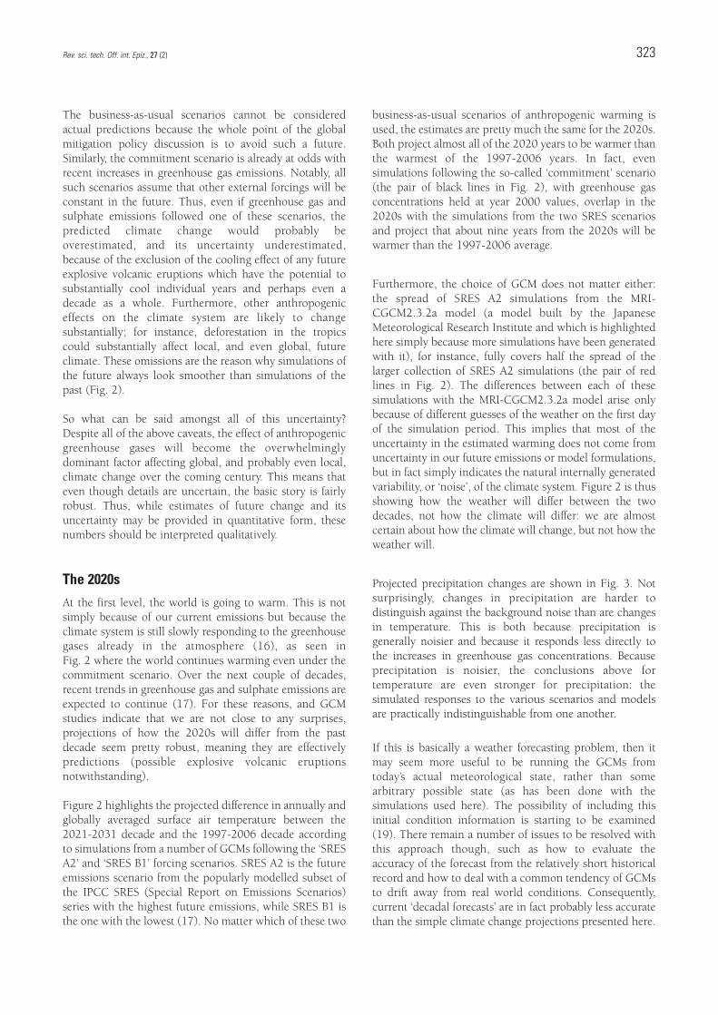
Figure 4 shows the global pattern of estimated warming ofthe 2020s from the 1997-2006 average. Unlike theannually averaged data shown in Fig. 2, the data shown inFig. 4 are decadally averaged for simplicity and in order tohighlight features. The maps are generated from 33 simulations from 10 GCMs following the SRES A1B

Rev. sci. tech. Off. int. Epiz., 27 (2)324

Fig. 4Maps of the decadally averaged surface temperature difference between the 2021-2030 decade and the 1997-2006 decadeThe left panel shows the very approximate 5th percentile at each grid cell from 33 simulations from 10 general circulation models following the SRES A1B scenario(a). For each 5° latitude by 5° longitude grid cell, the warming from the simulation closest to the 5th percentile of warming (the third coolest temperature difference) is shown. The right panel shows the approximate 95th percentile of warming (the third warmesttemperature differences)

(a) a ‘business-as-usual’ scenario between SRES A2 (with the highest emissions) and SRES B1 (with the lowest emissions)

Change (°C)

– 0.4 0.0 0.4 0.8 1.2 1.6

Change (°C)

– 0.4 0.0 0.4 0.8 1.2 1.6

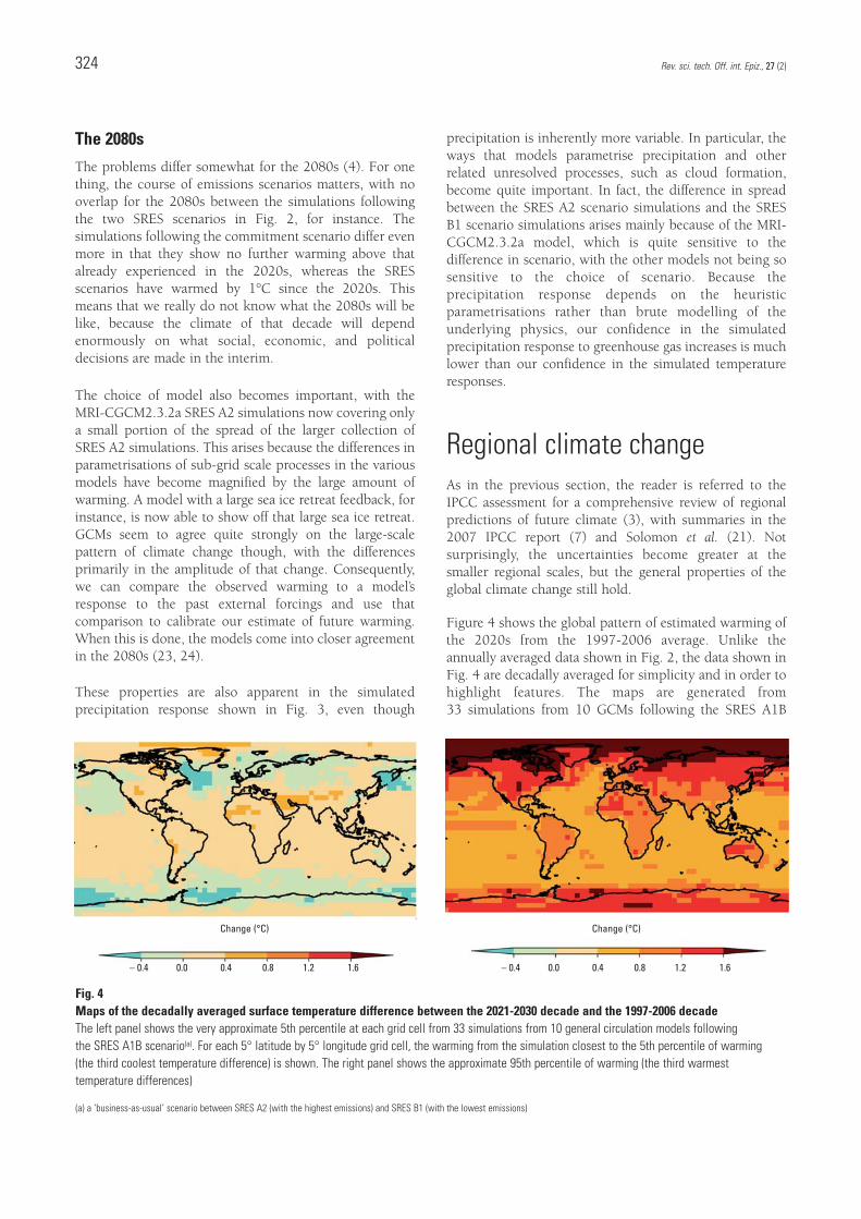
scenario, a business-as-usual scenario between SRES A2and SRES B1. The left-hand map shows the smallestamount of warming (or largest amount of cooling) that wemay reasonably expect to experience at any one location onthe 5° latitude by 5° longitude grid (~5% chance of beinglower), while the right-hand map shows the largest amountof warming we may reasonably expect to experience (~5%chance of being higher) at any one location. Each map isshowing the ‘reasonable’ (i.e. ~5% chance) extremecooling/warming at each location; it is much less likelythan 5% that all locations on the map would experiencesuch an extreme cooling/warming in any given simulation(or in the real world realisation that will happen), becausesome areas may experience greater warming than expectedand others less than expected. Warming is not guaranteedat any one location, although in all locations the odds arehigh that warming will occur. The greatest amount ofwarming is expected (and has been observed) over landand over high latitude regions; however, these locations arealso the ones with the highest uncertainty about the futurewarming. The changes projected for the 2080s (Fig. 5) aresimilar but considerably more significant, with it beingvery unlikely that any particular location will notexperience a noticeable warming.

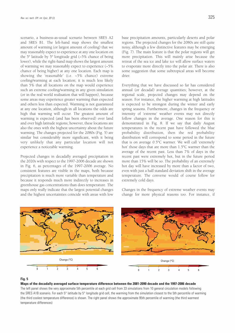
Projected changes in decadally averaged precipitation inthe 2020s with respect to the 1997-2006 decade are shownin Fig. 6, as percentages of the 1997-2006 average. Noconsistent features are visible in the maps, both becauseprecipitation is much more variable than temperature andbecause it responds much more indirectly to increases ingreenhouse gas concentrations than does temperature. Themaps only really indicate that the largest potential changesand the highest uncertainties coincide with areas with low

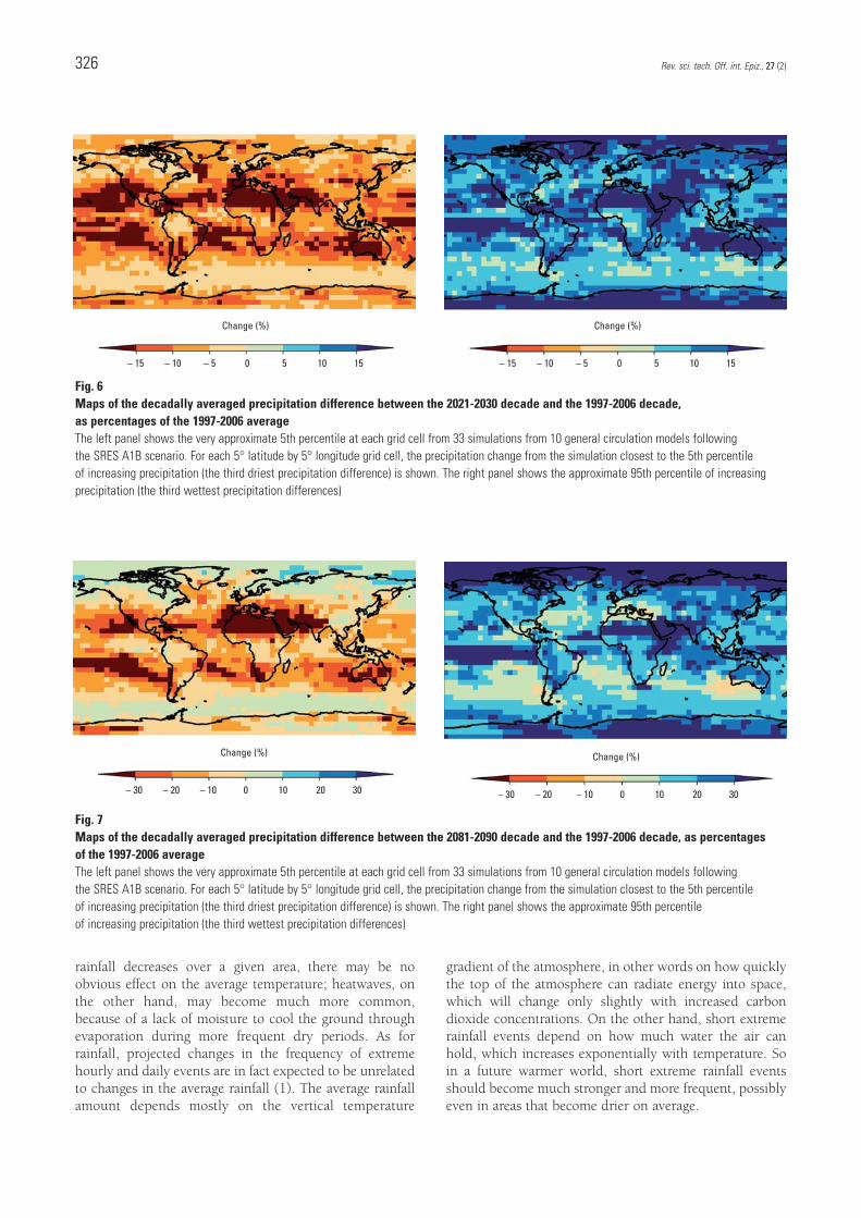
base precipitation amounts, particularly deserts and polarregions. The projected changes for the 2080s are still quitenoisy, although a few distinctive features may be emerging(Fig. 7). The main feature is that the polar regions will getmore precipitation. This will mainly arise because theretreat of the sea ice and lake ice will allow surface watersto evaporate more directly into the polar air. There is alsosome suggestion that some subtropical areas will becomedrier.

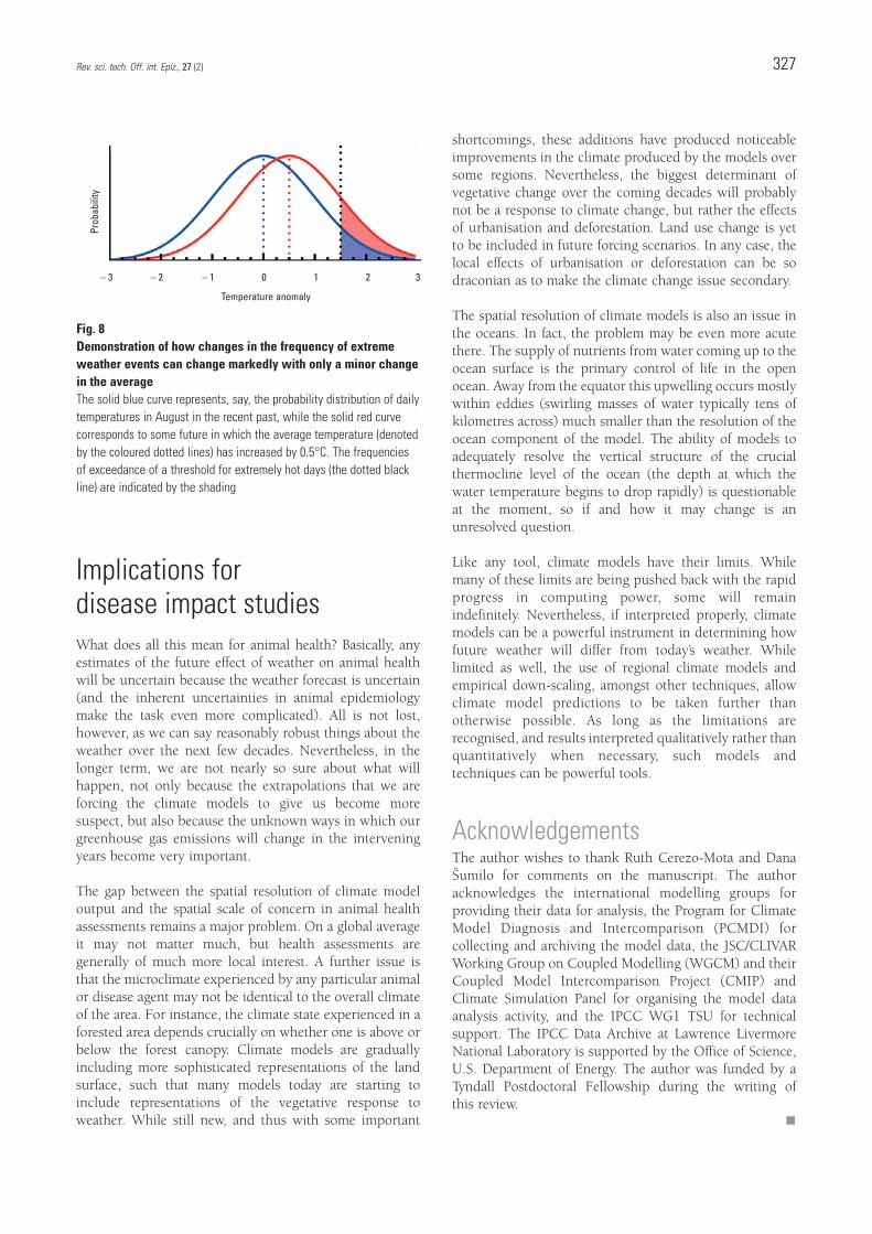
Everything that we have discussed so far has consideredannual (or decadal) average quantities; however, at theregional scale, projected changes may depend on theseason. For instance, the higher warming at high latitudesis expected to be strongest during the winter and earlyspring seasons. Furthermore, changes in the frequency orintensity of ‘extreme’ weather events may not directlyfollow changes in the average. One reason for this isdemonstrated in Fig. 8. If we say that daily Augusttemperatures in the recent past have followed the blueprobability distribution, then the red probabilitydistribution will correspond to some period in the futurethat is on average 0.5°C warmer. We will call ‘extremelyhot’ those days that are more than 1.5°C warmer than theaverage of the recent past. Less than 7% of days in therecent past were extremely hot, but in the future periodmore than 15% will be so. The probability of an extremelyhot day will have increased by more than a factor of two,even with just a half standard deviation shift in the averagetemperature. The converse would of course follow forextremely cold days.

Changes in the frequency of extreme weather events maychange for more physical reasons too. For instance, if

Rev. sci. tech. Off. int. Epiz., 27 (2) 325

Fig. 5Maps of the decadally averaged surface temperature difference between the 2081-2090 decade and the 1997-2006 decadeThe left panel shows the very approximate 5th percentile at each grid cell from 33 simulations from 10 general circulation models following the SRES A1B scenario. For each 5° latitude by 5° longitude grid cell, the warming from the simulation closest to the 5th percentile of warming (the third coolest temperature difference) is shown. The right panel shows the approximate 95th percentile of warming (the third warmesttemperature differences)

Change (°C)

0 1 2 3 4 5 6

Change (°C)

0 1 2 3 4 5 6

Rev. sci. tech. Off. int. Epiz., 27 (2)326

Fig. 6Maps of the decadally averaged precipitation difference between the 2021-2030 decade and the 1997-2006 decade, as percentages of the 1997-2006 averageThe left panel shows the very approximate 5th percentile at each grid cell from 33 simulations from 10 general circulation models following the SRES A1B scenario. For each 5° latitude by 5° longitude grid cell, the precipitation change from the simulation closest to the 5th percentile of increasing precipitation (the third driest precipitation difference) is shown. The right panel shows the approximate 95th percentile of increasingprecipitation (the third wettest precipitation differences)

Fig. 7Maps of the decadally averaged precipitation difference between the 2081-2090 decade and the 1997-2006 decade, as percentages of the 1997-2006 averageThe left panel shows the very approximate 5th percentile at each grid cell from 33 simulations from 10 general circulation models following the SRES A1B scenario. For each 5° latitude by 5° longitude grid cell, the precipitation change from the simulation closest to the 5th percentile of increasing precipitation (the third driest precipitation difference) is shown. The right panel shows the approximate 95th percentile of increasing precipitation (the third wettest precipitation differences)

rainfall decreases over a given area, there may be noobvious effect on the average temperature; heatwaves, onthe other hand, may become much more common,because of a lack of moisture to cool the ground throughevaporation during more frequent dry periods. As forrainfall, projected changes in the frequency of extremehourly and daily events are in fact expected to be unrelatedto changes in the average rainfall (1). The average rainfallamount depends mostly on the vertical temperature

gradient of the atmosphere, in other words on how quicklythe top of the atmosphere can radiate energy into space,which will change only slightly with increased carbondioxide concentrations. On the other hand, short extremerainfall events depend on how much water the air canhold, which increases exponentially with temperature. Soin a future warmer world, short extreme rainfall eventsshould become much stronger and more frequent, possiblyeven in areas that become drier on average.

Change (%)

– 15 – 10 – 5 0 5 10 15

Change (%)

– 15 – 10 – 5 0 5 10 15

Change (%)

– 30 – 20 – 10 0 10 20 30

Change (%)

– 30 – 20 – 10 0 10 20 30

Implications for disease impact studiesWhat does all this mean for animal health? Basically, anyestimates of the future effect of weather on animal healthwill be uncertain because the weather forecast is uncertain(and the inherent uncertainties in animal epidemiologymake the task even more complicated). All is not lost,however, as we can say reasonably robust things about theweather over the next few decades. Nevertheless, in thelonger term, we are not nearly so sure about what willhappen, not only because the extrapolations that we areforcing the climate models to give us become moresuspect, but also because the unknown ways in which ourgreenhouse gas emissions will change in the interveningyears become very important.

The gap between the spatial resolution of climate modeloutput and the spatial scale of concern in animal healthassessments remains a major problem. On a global averageit may not matter much, but health assessments aregenerally of much more local interest. A further issue isthat the microclimate experienced by any particular animalor disease agent may not be identical to the overall climateof the area. For instance, the climate state experienced in aforested area depends crucially on whether one is above orbelow the forest canopy. Climate models are graduallyincluding more sophisticated representations of the landsurface, such that many models today are starting toinclude representations of the vegetative response toweather. While still new, and thus with some important

shortcomings, these additions have produced noticeableimprovements in the climate produced by the models oversome regions. Nevertheless, the biggest determinant ofvegetative change over the coming decades will probablynot be a response to climate change, but rather the effectsof urbanisation and deforestation. Land use change is yetto be included in future forcing scenarios. In any case, thelocal effects of urbanisation or deforestation can be sodraconian as to make the climate change issue secondary.

The spatial resolution of climate models is also an issue inthe oceans. In fact, the problem may be even more acutethere. The supply of nutrients from water coming up to theocean surface is the primary control of life in the openocean. Away from the equator this upwelling occurs mostlywithin eddies (swirling masses of water typically tens ofkilometres across) much smaller than the resolution of theocean component of the model. The ability of models toadequately resolve the vertical structure of the crucialthermocline level of the ocean (the depth at which thewater temperature begins to drop rapidly) is questionableat the moment, so if and how it may change is anunresolved question.

Like any tool, climate models have their limits. Whilemany of these limits are being pushed back with the rapidprogress in computing power, some will remainindefinitely. Nevertheless, if interpreted properly, climatemodels can be a powerful instrument in determining howfuture weather will differ from today’s weather. Whilelimited as well, the use of regional climate models andempirical down-scaling, amongst other techniques, allowclimate model predictions to be taken further thanotherwise possible. As long as the limitations arerecognised, and results interpreted qualitatively rather thanquantitatively when necessary, such models andtechniques can be powerful tools.

AcknowledgementsThe author wishes to thank Ruth Cerezo-Mota and DanaŠumilo for comments on the manuscript. The authoracknowledges the international modelling groups forproviding their data for analysis, the Program for ClimateModel Diagnosis and Intercomparison (PCMDI) forcollecting and archiving the model data, the JSC/CLIVARWorking Group on Coupled Modelling (WGCM) and theirCoupled Model Intercomparison Project (CMIP) andClimate Simulation Panel for organising the model dataanalysis activity, and the IPCC WG1 TSU for technicalsupport. The IPCC Data Archive at Lawrence LivermoreNational Laboratory is supported by the Office of Science,U.S. Department of Energy. The author was funded by aTyndall Postdoctoral Fellowship during the writing of this review.

Rev. sci. tech. Off. int. Epiz., 27 (2) 327

Fig. 8Demonstration of how changes in the frequency of extremeweather events can change markedly with only a minor changein the averageThe solid blue curve represents, say, the probability distribution of dailytemperatures in August in the recent past, while the solid red curvecorresponds to some future in which the average temperature (denotedby the coloured dotted lines) has increased by 0.5°C. The frequenciesof exceedance of a threshold for extremely hot days (the dotted blackline) are indicated by the shading

Prob

abili

ty

Temperature anomaly

– 3 3– 2 2– 1 10

Rev. sci. tech. Off. int. Epiz., 27 (2)328

Le changement climatique attendu pour les prochaines années et ses conséquences sur les études d’impact sanitaire

D.A. Stone

RésuméL’auteur fait le point sur les prédictions que les spécialistes des modèlesclimatologiques sont à même de produire concernant l’évolution future duclimat. En effet, s’il est possible d’anticiper le changement climatique desprochaines décennies au moyen de modèles suffisamment robustes, lesprédictions visant un futur plus éloigné sont affectées par les incertitudes liéesà la structure du modèle climatologique et à l’évolution encore inconnue desémissions de gaz à effet de serre. Certains traits caractéristiques sontperceptibles au niveau régional ; néanmoins, à l’heure actuelle, les seulesinterprétations significatives de ces traits correspondent à des échellesspatiales trop vastes pour permettre d’anticiper avec justesse les effets sur lasanté animale du changement climatique. En conséquence, les prédictionsréalisées actuellement sur le changement climatique sont plutôt des indicationsque des descriptions exactes de l’évolution future.

Mots-clésChangement climatique – Climat – Météorologie – Modèle – Prédiction.

Cambios del clima previstos para los años venideros y su repercusión en el estudio de las consecuencias de las enfermedades

D.A. Stone

ResumenEl autor hace balance de la capacidad actual de los círculos científicos quetrabajan con modelos climáticos para formular predicciones relativas a la futuraevolución del clima. Aunque las predicciones para los próximos decenios sonrazonablemente sólidas, la anticipación referida a periodos más largos detiempo depende de inciertos factores ligados a la estructura de los modelosclimáticos y a la incógnita de cómo evolucionarán las emisiones de gases deefecto invernadero. En el plano regional destacan una serie de características,aunque ahora mismo sólo es posible interpretarlas cabalmente a una escalaespacial bastante mayor de lo requerido para hacer previsiones fiables de lafutura influencia del cambio climático en la salud animal. El corolario de todo elloes que ahora mismo no cabe tener por exactas, sino sólo meramente indicativas,las predicciones ligadas al cambio climático.

Palabras claveCambio climático – Clima – Elaboración de modelos – Meteorología – Predicción.

References1. Allen M.R. & Ingram W.J. (2002). – Constraints on future

changes in climate and the hydrologic cycle. Nature, 419, 224-232.

2. Christensen J.H., Carter T.R., Rummukainen M. &Amanatidis G. (2007). – Evaluating the performance andutility of regional climate models: the PRUDENCE project.Climat. Change, 81, 1-6.

3. Christensen J.H., Hewitson B., Busuioc A., Chen A., Gao X.,Held I., Jones R., Kolli R.K., Kwon W.T., Laprise R., Magaña Rueda V., Mearns L., Menéndez C.G., Räisänen J.,Rinke A., Sarr A. & Whetton P. (2007). – Regional climateprojections. In Climate Change 2007: The Physical ScienceBasis. Contribution of Working Group I to the FourthAssessment Report of the Intergovernmental Panel onClimate Change (S. Solomon, D. Qin, M. Manning, Z. Chen,M. Marquis, K.B. Averyt, M. Tignor & H.L. Miller, eds).Cambridge University Press, Cambridge, United Kingdom,847-940.

4. Cox P. & Stephenson D. (2007). – A changing climate forprediction. Science, 317, 207-208.

5. Delecluse P. (2008). – The origin of climate changes. In Climate change: the impact on the epidemiology and control of animal diseases (S. de la Rocque, S. Morand & G. Hendrickx, eds). Rev. sci. tech. Off. int. Epiz., 27 (2), 309-317.

6. International Ad Hoc Detection and Attribution Group(IDAG) (2005). – Detecting and attributing externalinfluences on the climate system: a review of recent advances.J. Climate, 18, 1291-1314.

7. Intergovernmental Panel on Climate Change (IPCC) (2007). – Summary for policymakers. In Climate Change2007: The Physical Science Basis. Contribution of WorkingGroup I to the Fourth Assessment Report of theIntergovernmental Panel on Climate Change (S. Solomon, D. Qin, M. Manning, Z. Chen, M. Marquis, K.B. Averyt, M. Tignor & H.L. Miller, eds). Cambridge University Press,Cambridge, United Kingdom, 1-18.

8. Knight C.G., Knight S.H.E., Massey N., Aina T., Christensen C., Frame D.J., Kettleborough J.A., Martin A.S.P.,Sanderson B., Stainforth D.A. & Allen M.R. (2007). –Association of parameter, software, and hardware variationwith large-scale behaviour across 57,000 climate models.Proc. natl Acad. Sci. USA, 104, 12259-12264.

9. Le Treut H., Somerville R., Cubasch U., Ding Y., Mauritzen M., Mokssit A., Peterson T., Prather M. et al.(2007). – Historical overview of climate change science. In Climate Change 2007: The Physical Science Basis.Contribution of Working Group I to the Fourth AssessmentReport of the Intergovernmental Panel on Climate Change (S. Solomon, D. Qin, M. Manning, Z. Chen, M. Marquis, K.B. Averyt, M. Tignor & H.L. Miller, eds). CambridgeUniversity Press, Cambridge, United Kingdom, 93-127.

10. Leung R.L., Mearns L.O., Giorgi F. & Wilby R.L. (2003). –Regional climate research: needs and opportunities. Bull. Am.Meterol. Soc., 84, 89-95.

11. Lorenz E. (1993). – The Essence of Chaos. UCL Press,London, 227 pp.

12. McAvaney B.J., Covey C., Joussaume S., Kattsov V., Kitoh A.,Ogana W., Pitman A.J., Weaver A.J., Wood R.A., Zhao Z.C. et al. (2001). – Model evaluation. In Climate Change 2001:The Scientific Basis. Contribution of Working Group I to theThird Assessment Report of the Intergovernmental Panel onClimate Change (J.T. Houghton, Y. Ding, D.J. Griggs, M. Noguer, P.J. van der Linden, X. Dai, K. Maskell & C.A. Johnson, eds). Cambridge University Press, Cambridge,United Kingdom, 881 pp.

13. McGuffie K. & Henderson-Sellers A. (2005). – A ClimateModeling Primer. John Wiley & Sons, New York, 280 pp.

14. Mearns L.O., Giorgi F., Whetton P., Pabon D., Hulme M. &Lal M. (2003). – Guidelines for use of climate scenariosdeveloped from regional climate model experiments.Technical report, IPCC Task Group on Data and ScenarioSupport for Impact and Climate Analysis (TGICA). Availableat: http://www.ipccdata.org/guidelines/dgm_no1_v1_10-2003.pdf (accessed on 23 October 2007).

15. Meehl G.A., Stocker T.F., Collins W.D., Friedlingstein P., Gaye A.T., Gregory J.M., Kitoh A., Knutti R., Murphy J.M.,Noda J., Raper S.C.B., Watterson I.G., Weaver A.J., Zhao Z.C.et al. (2007). – Global climate projections. In Climate Change2007: The Physical Science Basis. Contribution of WorkingGroup I to the Fourth Assessment Report of theIntergovernmental Panel on Climate Change (S. Solomon, D. Qin, M. Manning, Z. Chen, M. Marquis, K.B. Averyt, M. Tignor & H.L. Miller, eds). Cambridge University Press,Cambridge, United Kingdom, 747-845.

16. Meehl G.A., Washington W.M., Collins W.D., Arblaster J.M.,Hu A., Buja L.E., Strand W.E. & Teng H. (2005). – How much more global warming and sea level rise? Science,307, 1769-1772.

17. Nakićenović N., Alcamo J., Davis G., de Vries B., Fenhann J.,Gaffin S., Gregory K., Grübler A., Jung T.Y., Kram T., La Rovere E.L., Michaelis L., Mori S., Morita T., Pepper W.,Pitcher H., Price L., Raihi K., Roehrl A., Rogner H.H.,Sankovski A., Schlesinger M., Shukla P., Smith S., Swart R.,van Rooijen S., Victor N. & Zhou D. (2000). – IPCC SpecialReport on Emissions Scenarios. Cambridge University Press,Cambridge, United Kingdom, 599 pp.

18. Schär C., Vidale P.L., Lüthi D., Frei C., Häberli C., LinigerM.A. & Appenzeller C. (2004). – The role of increasingtemperature variability in European summer heatwaves.Nature, 427, 332-336.

Rev. sci. tech. Off. int. Epiz., 27 (2) 329

19. Smith D.M., Cusack S., Colman A.W., Folland C.K., Harris G.R. & Murphy J.M. (2007). – Improved surfacetemperature prediction for the coming decade from a globalclimate model. Science, 317, 796-799.

20. Soden B.J. & Held I.M. (2006). – An assessment of climatefeedbacks in coupled ocean-atmosphere models. J. Climate,19, 3354-3360.

21. Solomon S., Qin D., Manning M., Alley R.B., Berntsen T.,Bindoff N.L., Chen Z., Chidthaisong A., Gregory J.M., Hegerl G.C., Heimann M., Hewitson B., Hoskins B.J., Joos F.,Jouzel J., Kattsov V., Lohmann U., Matsuno T., Molina M.,Nicholls N., Overpeck J., Raga G., Ramaswamy V., Ren J.,Rusticucci M., Somerville R., Stocker T.F., Whetton P., Wood R.A., Wratt D. et al. (2007). – Technical summary. In Climate Change 2007: The Physical Science Basis.Contribution of Working Group I to the Fourth AssessmentReport of the Intergovernmental Panel on Climate Change (S. Solomon, D. Qin, M. Manning, Z. Chen, M. Marquis, K.B. Averyt, M. Tignor & H.L. Miller, eds). CambridgeUniversity Press, Cambridge, United Kingdom, 19-91.

22. Stone D.A. & Allen M.R. (2005). – Attribution of globalsurface warming without dynamical models. Geophys. Res.Lett., 32, L18711. DOI: 10.1029/2005GL023682.

23. Stone D.A., Allen M.R. & Stott P.A. (2007). – A multi-modelupdate on the detection and attribution of global surfacewarming. J. Climate, 20, 517-530.

24. Stott P.A., Mitchell J.F.B., Allen M.R., Delworth T.L., Gregory J.M., Meehl G.A. & Santer B.D. (2006). –Observational constraints on past attributable warming andpredictions of future global warming. J. Climate, 19, 3055-3069.

25. Wilby R.L., Charles S.P., Zorita E., Timbal B., Whetton P. &Mearns L.O. (2004). – Guidelines for use of climate scenariosdeveloped from statistical downscaling methods. Technicalreport, IPCC Task Group on Data and Scenario Support forImpact and Climate Analysis (TGICA). Available at:http://ipcc-ddc.cru.uea.ac.uk/guidelines/StatDown_Guide.pdf (accessed on 23 October 2007).

Rev. sci. tech. Off. int. Epiz., 27 (2)330