Precision-Driven Hybrid Control for 3D Microassembly

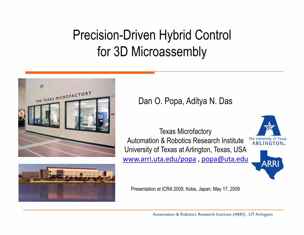
Precision-Driven Hybrid Control for 3D Microassembly

Dan O Popa Aditya N DasDan O. Popa, Aditya N. Das

Texas MicrofactoryTexas MicrofactoryAutomation & Robotics Research Institute

University of Texas at Arlington, Texas, USAwww.arri.uta.edu/popa , [email protected]/p p , p p @

Presentation at ICRA 2009, Kobe, Japan, May 17, 2009p y

Texas Microfactory at ARRI

DFW

from concept to productionARRI TMfrom concept to productionARRI TM

Texas Microfactory Research Program: Smart Micromachines

NEXT GENERATION ROBOTICS

Humanoids | Precision Microrobotics | Distributed Robotics

SMART MICROMACHINES

Smart Materials | Smart Devices | Smart Networks

MICROMANUFACTURING

Packaging | Assembly | Testing | Reliability

Texas Microfactory Technical Focus:Robotics and Microengineeringg g

μmachines

μdevices

μmachines

μνrobotics

μengineering

Packaging

PrecisionDesign

Robotics

Modularity Packaging

Sensors, Actuators, Power Scavengers

Materials

y

Interactivity

Structural Health Management

Biomimetic Microrobotic Swarms

Humanoids

Outline of Presentation

• Introduction/ Motivation: Microassembly with Precision Robotics

• Hybrid 3D Microassembly and a few applications

• Precision Robotics: precision metrics

• Yield guarantees and precision metrics: HYAC Condition and RRA Rules

• Hybrid Control for hybrid microassembly

bl h l d l•Microassembly Systems (Physical and Virtual)

• Proposed Hybrid Controller and Path Planner

i i d i l l• Simuation and Experimental Results

• Conclusion and Future Work

MicroAssembly As a Manufacturing Method

Serial

Manual

Teleoperated May use multiscale, multirobot platforms with microgrippers

Probes on manual stages

platforms with microgrippers.Vary in throughout and yield.

Microgripper arrays

Automated

Deterministic

Stochastic

Flip Chip Bonding/Stacking

Self assembly

Parallel

Distributed ArrayDeterministic assembly:

- Weaknesses: expensive equipment, slow, not scalable to many parts- Strengths: can build complex structures can obtain high yield by “tweaking” performance- Strengths: can build complex structures, can obtain high yield by tweaking performance

Stochastic assembly:- Weaknesses: only simple assemblies, high yield takes a long time- Strengths: scalable to many parts, simple equipmentThis presentation proposes a precision-adjusted path-planning and hybrid control strategy to improve theThis presentation proposes a precision adjusted path planning and hybrid control strategy to improve the yield and speed of serial, automated microassembly.

Deterministic Stochastic

MicroAssembly: ContextDeterministic Stochastic

Top-downSerial

Assembly of small components is difficult :• Position/process

interdependencyS li f h i

Bottom-up

Parallel

Self assembly

• Some scaling of physics• Stringent tolerance• High precision requirements

for equipment• Time sensitive

10-6 10-7 10-8 10-910-3 10-4 10-510-2

in meters

• Limited sensing and dexterity• Dynamical effects causing

vibrations

Effect of gravitational forces

Effect of surface forces

Ki i /D i l F C l

D.O. Popa, H. Stephanou, “Micro and meso scale robotic assembly”, in SME Journal of Manufacturing Processes, Vol. 6, No.1, 2004, 52‐71.

Kinematic/Dynamic control Force Control

Assembly time

Predictability (yield)

Motivation: Automated 3D MicroassemblyAutomated , Serial or Parallel Hybrid Microassembly is a viable pathway for mass production of microsystems with modular component dimensions above ?0 microns.

ffAutomated Deterministic Microassembly is difficult and requires careful consideration of several important tradeoffs:

i. Serial microassembly is slow but can have high yield and construct complex 3D shapes for part dimensions above ?0 microns.

ii. Open-loop control with calibration or models can be used, but:i. If it relies on high repeatability it usually leads to both

expensive and bulky hardware.

ii If it relies on compliance then it must be engineered intoii. If it relies on compliance then it must be engineered into parts and end-effectors.

iii. Closed-loop feedback control can provide higher precision but:i. Usage in quasi-static operation decreases throughput

(“ )(“look and move”).

ii. Usage in dynamic operation leads to vibrations which are of higher frequency than the sensor or control system bandwidth.

iii. Workspace is limited, this applies to sensors , actuators and end-effectors sharing the workspace.

Examples of 3D microassembly from Texas Microfactory

Our Approach: Maximize Assembly Yield, then Speed, then Cost

Key factors driving the assembly yield at small scales:Precision requirements (how accurate the robots are)Tolerance requirements (how accurate the parts are)Throughput requirements (how fast we want to assemble)Interaction forces between parts (how parts interact)Sensory vs. sensorless ability (what kind of sensors do we have available)Part design (are the parts “assemblable”?).

The goal of our work is to formulate a framework with quantitative metrics and decision rules forThe goal of our work is to formulate a framework with quantitative metrics and decision rules for microassembly cells:

‐ Design rules – how many robots, heteroceptive sensors, their specs, etc.‐ Hybrid Control rules – when to switch between controllersPath Planning rules which paths to follow to increase precision‐ Path Planning rules – which paths to follow to increase precision

Our approach

i. High yield assembly guarantees from “new” precision metrics

ii. Precision adjusted hybrid control for faster throughput through a “complexity index”j y g p g p y

iii. “Precise” path planning algorithms to reduce sensor cost and ensure higher precision

iv. Complex 3D simulation of microassembly in a virtual world with high realism for planning and validation before being ported to the assembly system.

Mi / f t i i t f t f d t f b i t f t t t ith

Background: making small things with automated machines• Micro/nano manufacturing consists of a set of processes used to fabricate features, components, or systems with

dimensions described in micrometers or nanometers.

• In any endeavor where small things are made, characterized, assembled, tested, or used, it is necessary to apply the fundamental practices of precision engineering . However, these practices are rooted in pre‐20‐th century technology.

• Internationally, metrology standards are set by ISO (International Organization for Standardization). In the USA standards are set by NIST and ANSI. They have set precision standards for automated machines, including robotsrobots.

• CNC machine tool industry have applied these concepts routinely, but traditionally, their precision relies on the mechanical structure of the system making them very bulky.

• Intelligent Robotics offers the possibility to reduce the size of micro/nano manufacturing systems but precisionIntelligent Robotics offers the possibility to reduce the size of micro/nano manufacturing systems, but precision concepts and standards in robotics are rarely followed.

• As a 21th century technology, Microrobotics needs new precision concepts beyond the 19th century ones.

• We propose a new precision framework for top‐down robotic assembly systems with guaranteed high yields,We propose a new precision framework for top down robotic assembly systems with guaranteed high yields, reasonable high speeds, and reasonable low cost.

• Presentation argues that this will require a new set of robotics‐centric precision metrics, other than the conventional definitions of accuracy, repeatability, resolution.

Conventional Precision MetricsResolution: The smallest output increment that a machine can perform.

Repeatability: The ability of a machine to return to the same state over many cycling attempts.

good accuracy

Poor

Accuracy: The maximum expected difference between the actual and the ideal (desired) output for a given input

In Metrology, Resolution and Accuracy are mean values, while

repeatability

gy, y ,Repeatability is a statistical distribution.

Outputs vary, and examples could be, motion (position), measurement (distance, angle, temperature, intensity, etc), parts produced (tolerance of parts).

poor accuracy

good repeatability

For Precision Robotics, these metrics should :

• All be statistical variables following Gaussian Probability Density Functions.

• Be metrics related to the end‐effector, as often times they are confused with similar metrics at other points of measurement.

• Be redefined to closely match the type of controller sensor and actuator

good accuracy

good repeatability

Be redefined to closely match the type of controller, sensor and actuator system used.

Tradeoffs related to measurement location to the precision attainable by robots

Direct: Measurement of motion at the tool‐ Pros: few sources of errors, related to the tool position measurement instrument only.‐ Cons: more complex measurement sensors, servo loop controller K2 more complexIndirect: Measurement of motion at the joints‐ Cons: lots of sources of errors: measurement instrument error (for instance joint encoders), kinematic parameters, other unknown factors (friction, backlash, temperature variation). Inverse model construction needed. ‐ Pros: Calibration loop controller K1 simple, model needed only once.

Both direct and indirect measurements are needed for high precision machines.

Part/tool position measurement feedback

‐

RobotMotors

feedbackDesired end‐effector position Xd

K2

Inverse i i d l K1

+Ex=Xd‐X

U F

Servo Loop

RobotEnd‐effector position X

MotorsJoint position feedback Q

‐Kinematic Model

Desired Joint position Qd

K1 +Eq=Qd‐Q

Calibration Loop / Open Loop Operation

3D Microassembly

Gripper frame

part frames f3f4

K(q)‐ pose

f2

f3f4

f1

Silicon die with micropartsGlobal frame Fiducial

frame

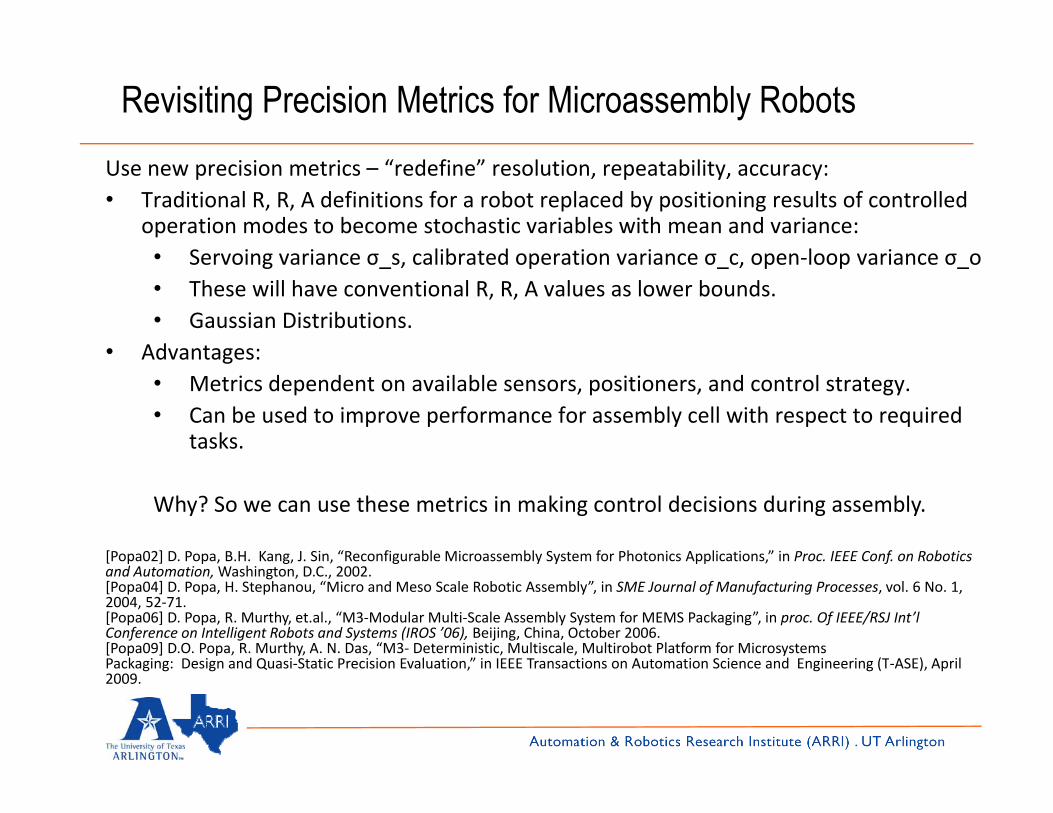
Revisiting Precision Metrics for Microassembly RobotsUse new precision metrics – “redefine” resolution, repeatability, accuracy:• Traditional R, R, A definitions for a robot replaced by positioning results of controlled

operation modes to become stochastic variables with mean and variance:S i i lib t d ti i l i• Servoing variance σ_s, calibrated operation variance σ_c, open‐loop variance σ_o

• These will have conventional R, R, A values as lower bounds.• Gaussian Distributions.

• Advantages:Advantages: • Metrics dependent on available sensors, positioners, and control strategy.• Can be used to improve performance for assembly cell with respect to required

tasks.

Why? So we can use these metrics in making control decisions during assembly.

[Popa02] D. Popa, B.H. Kang, J. Sin, “Reconfigurable Microassembly System for Photonics Applications,” in Proc. IEEE Conf. on Robotics[Popa02] D. Popa, B.H. Kang, J. Sin, Reconfigurable Microassembly System for Photonics Applications, in Proc. IEEE Conf. on Robotics and Automation, Washington, D.C., 2002.[Popa04] D. Popa, H. Stephanou, “Micro and Meso Scale Robotic Assembly”, in SME Journal of Manufacturing Processes, vol. 6 No. 1, 2004, 52‐71.[Popa06] D. Popa, R. Murthy, et.al., “M3‐Modular Multi‐Scale Assembly System for MEMS Packaging”, in proc. Of IEEE/RSJ Int’l Conference on Intelligent Robots and Systems (IROS ’06), Beijing, China, October 2006.[Popa09] D.O. Popa, R. Murthy, A. N. Das, “M3‐ Deterministic, Multiscale, Multirobot Platform for Microsystems Packaging: Design and Quasi Static Precision Evaluation ” in IEEE Transactions on Automation Science and Engineering (T ASE) AprilPackaging: Design and Quasi‐Static Precision Evaluation, in IEEE Transactions on Automation Science and Engineering (T‐ASE), April 2009.

New Precision Metrics1. Accuracy: The robotic system is commanded to place the end‐effector at a designated position

in 3D‐space which may involve translation and/or rotation in R6. A fixed or mobile sensor (for instance, an optical microscope) is used to determine the error between actual and desired position of the end‐effector. The error distribution with respect to the sensor gives the measure position of the end effector. The error distribution with respect to the sensor gives the measure for accuracy, σacc.(Note: conventionaly, accuracy is a mean value, not a distribution). After repeated motions (regardless of control method)

⎞⎛( ) ( ) ( )

⎟⎞

⎜⎛

⎟⎟⎠

⎞⎜⎜⎝

⎛⎟⎟⎠

⎞⎜⎜⎝

⎛Δ++≤

∑

∑=

∞→

N

N

jjNSkSPkSkaccuracy qK

Nqq

1

2222_

1

)(1limmin σσσ

Sensor frame localization uncertainties are σSk, and its measurement uncertainty of the k‐th DOF of part P is given by σSPk, ΔKj is the variation in position measurement j of the k‐th DOF

⎟⎟⎠

⎞⎜⎜⎝

⎛++≤ ∑

=∞→ j

jNkaccuracy qKN

SkqSPkqK1

_ )(1lim)())(()( μμ

p g y SPk, j p jabout its mean.

Go one step further: use open loop control with an nominal inverse model to drive the system when making these measurements, σo=σaccuracy E.g. define accuracy as the robot intrinsic g , o accuracy. g f yprecision as measured by heteroceptive sensors, but without using this data in any way.

New Precision Metrics

2. Calibrated Model:

Calibration Error is the uncertainty value of the forward kinematic map K(q) averaged over the set of all features part σKk(q). This uncertainty depends on the number of measurements N, the number of features Q, and the sensor uncertainty for all measurements, e.g.

)],,,,([),,,(~

QkNqKEqkQNK SPkiσ=

Clearly,

~)())(()(lim)(kl b SkqSPkqkQNKqK μμ +≥=

ZYXp Zp

Yc

Zc

222

,

2_

,_

)(lim)(

),())((),,,(lim)(

SkSPkKkQNkncalibratio

QNkncalibratio

qq

SkqSPkqkQNKqK

σσσσ

μμ

+≥=

+≥=

∞→

∞→ op

YoXc


2. Repeatability: The robotic system is commanded to place the end‐effector alternatively between two predefined but arbitrary points in 3D‐space (corresponding to two respective joint p y p p ( p g p jcoordinate vectors) one of which is measured through a sensor. The error distribution with respect to the sensor gives the measure for repeatbility, σrep.

(Note: this corresponds to the traditional definition of repeatablility or precision)p p y p

))))((1(lim)((min)(1

222_ ∑

=∞→

Δ+≤N

jjNSPkSkrepeat qK

Nqq σσ

When we use open loop control with a calibrated inverse nominal model to drive the system, the positioning uncertainty is given by:

222tlib ti σσσ +=

Assuming perfect calibration data, σc=σrep. In practice, we obtain “good enough” calibration data when it is below its repeatability.

repeatncalibratioc σσσ +


3. Resolution:We define the resolution of the robot system as the minimum increment that the manipulator can sense and execute in Cartesian space, 3σres transformed into a distribution with a mean 3σres and uncertainty σres given by:

(Note: this is typically one or the other, usually the minimum increment that the robot can

)),3/)(max(min()(_ SPkkkres qKq σσ Δ≤

execute).During servo operations:

)()()()( 11 qKqJqKqJq SoS λλ −≈−= −−•

Factor in steady state control error:

)()( qKqK ss λ−≈•

When we use closed‐loop servoing to drive the system, the final positioning

2_

22statesteadyrepeats σσσ +=

uncertainty is given by σs=σres

R.R.A precision design rules for designing top-down assembly systems with high yield, high speed, low cost

Consider an assembly with tolerance Δk12 along DOF k, between a part 1 manipulated from position A, and part 2 fixed on a substrate at position B.

• Rule1: If the use of fixtures at taught locations along DOF k, will cause the assembly operation to succeed 99%+ of the time, will incur a speed cost C1=f1(AB), where f1is a monotonically increasing function of the distance between A and B, and a sensor/feedback cost C2=0 (no heteroceptive sensors or feedback)

ok σ312 >Δ

2 ( p )• Rule 2: If the use of servoing along DOF k will cause the assembly operation to succeed 99%+ of the time, will incur a speed cost C1=f1(AB), and a sensor/feedback cost C2=f2(AB).• Rule 3: If the use of calibration along DOF k with sufficient calibration points N,

sk σ312 >Δ

ck σ312 >Δ g p ,will cause the assembly operation to succeed 99%+ of the time, will incur a speed cost C1= f1(NAB) , and a sensor/feedback cost C2= f3(AB).

The monotonically increasing functions fi are assembly system designer’s choice.

cσ12

y g i y y g

Assembly planning can be done to decide how to switch between the three modes of operation, by minimizating a weighted index W=w1C1+w2C2, where wi are positive design weights.g

Precision Robotic Workcells: M3, μ3 and N3Precision metrics were used in conjunction with assembly workcell design parameters to optimize yield, speed and reduce robot complexity, allowing:

- Increase assembly speed due to precision-adjusted hybrid control (e.g. switchingIncrease assembly speed due to precision adjusted hybrid control (e.g. switching between different operation modes depending on precision requirements).- Assembly yield guarantees built into control strategy and design of workcell.- Selection of sensors and actuators just “good enough” to achieve desired preformance.- Reduction of accuracy to workcell volume ratios as scales reduce- Reduction of accuracy to workcell volume ratios as scales reduce- Automated assembly with better yield than teleoperated assembly.

Hardware incarnations at Texas Microfactory - three progressively smaller workcells:• M³– 4 precision robots, large workspace, micron-level resolution and few microns accuracy• μ³ - 3 precision robots, small workspace, nm-level resolution, sub-micron accuracy.μ p , p , , y• N³ – 10-100 microscale robots on a wafer, nm-level resolution, 1 micron accuracy.

M³: Macro-Meso-Micro Packaging Platformfor devices with cm/mm part size and μm tolerance

• Four precision robots sharing a common workspace, with multiple end effectors: microgrippers zoom

Laser solder reflow (delivery optics) – 3DOF

Zoom‐camera system – 2DOF

Gripper Manipulator 4DOF

Hot plate for die attach

with multiple end‐effectors: microgrippers, zoom microscope, laser for solder reflow.

• Work volume of approximately O(1 m3), robots with dimensions of O(10‐1~10‐2m), handles parts of size

4DOF

Tool tray withquickchange end‐effectors

dimensions of O(10 10 m), handles parts of size O(10‐2~10‐4m), and achieves accuracies in the scale of O(10‐4~10‐6 m).

Parts tray

Fine manipulator3DOF

Packaged MOEMS device using the M³ Schematic and Control System Diagram of M³using the M Schematic and Control System Diagram of M

Example Application: Packaging of MOEMS Device

Assembly and packaging of heterogeneous MOEMS device.

Top Chip

MOEMS Die

Sn/Au Preform

Carrier

Optical Fiber

M³ Design “RRA” Rules

Manipulator accuracy < tolerance required (fiber to package, In preform insertion)

Manipulator repeatability < tolerance required (die

Use fixtures, open loop

Use calibration open loop

O i l fib k l b d

Manipulator resolution < tolerance required (fiber to die)

attach, top chip attach) Use calibration, open loop

Use servoing, closed loop

Optical fiber to package tolerance budget

ΔX ΔY ΔZ Δθ Δϕ ΔΨ

Open Loop with nominal model

D.O. Popa, R. Murthy, A. N. Das, “M3‐

FIBER TO PACKAGE

300 300 186 1.73 1.73 -

(µm) (µm) (µm) (YAW)deg

ϕ(PITCH)

deg(ROLL)

deg

Deterministic, Multiscale, Multirobot Platform for Microsystems Packaging: Design and Quasi‐Static Precision Evaluation,” in IEEE Transactions on Automation Science and Engineering (T‐ASE) April 2009

FIBER TO TRENCH

4 4 25 0.2 - -

ASE), April 2009.

Servoing (Repeatability > 7.9 microns) Open Loop w/calibration

μ³: Meso-Micro-Nano Assembly Platformfor MEMS with mm/μm part size and nm tolerance

• Three precision end‐effectors sharing a common workspace with a total of 19 DOF.

• Accomplishes high speed compliant MEMS

Three μ³ end‐effectors share a common 8 cm³‐ size workspace

assembly with high yield guarantees.

• Has a O(10‐2 m) workspace, robots with dimensions O(10‐2~10‐3m), handles MEMS components of O(10‐3~10‐5 m) in size, achieves O(10‐6~10‐7 m) accuracy. p10 m) in size, achieves O(10 10 m) accuracy.

Silicon MEMS microgrippers and microsnap fastners Assembled MOEMS: scanning mirrors, micro‐ball lenses, microinterferometer

1mmx1mm Cu coupon assembled onto a MEMS die using the μ³.

A Das P Zhang WH Lee D Popa H Stephanou “µ³: Multiscale Deterministic Micro‐Nano Assembly System for Construction of On‐A. Das, P. Zhang, W.H. Lee, D. Popa, H. Stephanou, µ : Multiscale, Deterministic Micro Nano Assembly System for Construction of OnWafer Microrobots,” in Proceedings of ICRA 2007.

High Yield Compliant MEMS Assembly

Misalignment design threshold for DOF λ(probability of assembly)

k1σPart location errork2σ 222 +≥

High Yield Assemblability Condition(H.Y.A.C.) for 99% Yield

Part location errork2Robot positioning error k3σ

23

22

21 kkk σσσ +≥

Repeated Zyvex Connector Assemblies with High Yield Microspectrometer Assemblyy g y

R Murhy A N Das D O Popa “High Yield Assembly of Compliant MEMS Snap Fasteners ” in Proc ofR. Murhy, A.N. Das, D. O. Popa, High Yield Assembly of Compliant MEMS Snap Fasteners, in Proc. of ASME Int’l Conf. on Micro and Nano Systems, August 2008.

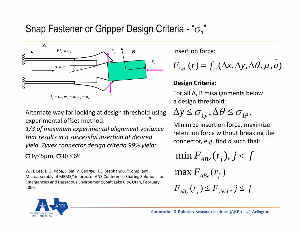
Snap Fastener or Gripper Design Criteria - “σ1”

),,,,()(_ayxfrF riABi μθΔΔΔ=

5aEIs =

xF1a=α

BA

yF Insertion force:

432 ,, atawal sss ===

Design Criteria:

For all A, B misalignments below a design threshold:

Minimize insertion force, maximize i f i h b ki h

,, 11 θσθσ ≤Δ≤Δ yya design threshold:

Alternate way for looking at design threshold using experimental offset method: 1/3 of maximum experimental alignment variance

_a_a

retention force without breaking the connector, e.g. find a such that:

fjrF jABx <),(min

1/3 of maximum experimental alignment variance that results in a successful insertion at desired yield. Zyvex connector design criteria 99% yield:

σ1y≤5µm, σ1θ ≤6º fjjABx ),()(max fABz rF

fjFrF ≤≤)(

W. H. Lee, D.O. Popa, J. Sin, V. George, H.E. Stephanou, “Compliant Microassembly of MEMS,” in proc. of ANS Conference Sharing Solutions for Emergencies and Hazardous Environments, Salt Lake City, Utah, February 2006. fjFrF yieldjABy ≤≤ ,)(

,

Part Fixturing Tolerance – “σ2”

Depends on part and thether designs and how they are brokenare broken

Data set: 62 samplesσ2y≤2.89µmσ2θ ≤4º

W. H. Lee, M. Dafflon, H.E. Stephanou, Y.S. Oh, J. Hochberg, and G. D. Skidmore, “Tolerance analysis of placement distributions in tethered micro‐, y pelectro‐mechanical systems components,” in Proceedings of IEEE International Conference on Robotics and Automation, May, 2004.

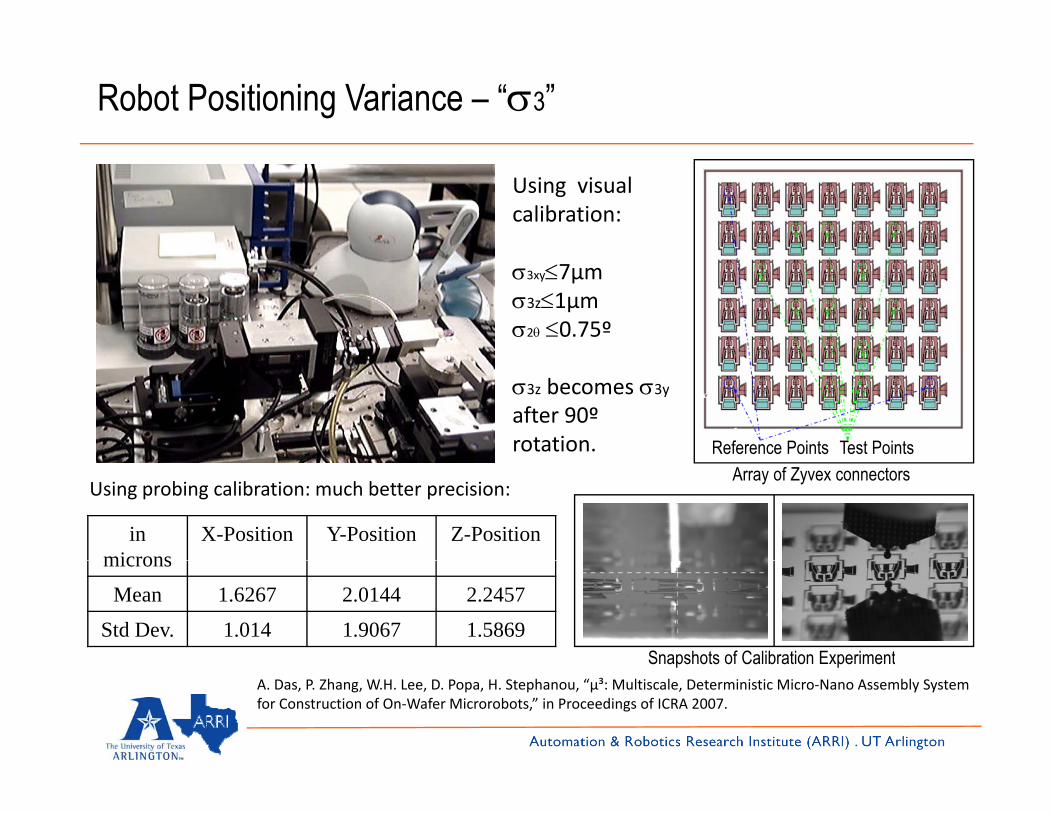
Robot Positioning Variance – “σ3”

Using visualcalibration:

σ3xy≤7µm σ3z≤1µmσ2θ ≤0.75º

Reference Points Test Points

σ3z becomes σ3y

after 90º rotation.

in microns

X-Position Y-Position Z-Position

Array of Zyvex connectorsUsing probing calibration: much better precision:

microns

Mean 1.6267 2.0144 2.2457

Std Dev. 1.014 1.9067 1.5869Snapshots of Calibration Experiment

A. Das, P. Zhang, W.H. Lee, D. Popa, H. Stephanou, “µ³: Multiscale, Deterministic Micro‐Nano Assembly System for Construction of On‐Wafer Microrobots,” in Proceedings of ICRA 2007.

Snapshots of Calibration Experiment

Assembled FTIR MicrospectrometerAdvantages:

• Micro-optical bench configured on 1cm x 1cm SOI Si die

for visible and NIR range.

• Integrated electro thermal MEMS actuator on die

• Simple 2½D MEMS fixtures with compliant snap

fasteners fabricated by DRIE

Michelson interferometer based Fourier Transform spectrometer by ARRI, University of Texas at Arlington.

• Off-the-shelf micro optical components

• Automated 3D Microassembly of micro-optical fixtures

•Ability to integrate a photo detector, laser or couple the

optical bench to a fiber

•Simple On board electronics for actuation and DAQ

•Can be packaged in 3cm x 3cm x 3cm footprint with

approximately 30grams total weight

•10nm resolution at 650nm and 30nm at 1550nm.A.N. Das, J. Sin, D. O. Popa, H.E. Stephanou, “Design and Manufacturing of aFourier Transform Microspectrometer,” in Proc. of IEEE Int’l Conf. onNanotechnology, August 2008.

ARRIpede MicrocrawlerSystem Specifications:• Volume = 1.5cm X 1.5cm X 1.5cm• Weight ~ 4g• Velocity 1~3mm/s• Velocity=1~3mm/s•Payload~9g•3 degrees of freedom (XYθ)

Micromechanical details• Constructed using Si MEMS BellyLegs• Electrothermal actuator arrays fabricated on belly• 21/2 D legs assembled to actuators via micro snap‐fasteners• Stick slip based motion

y

Stick slip based motion

Leg

Actuator

900µmJoint

R. Murthy, A.N.Das, D. O. Popa, “ARRIpede: A Stick‐Slip Micro Crawler/Conveyer Robot Constructed Via 2 ½D MEMS Assembly,” in Proc. of 2008 IEEE Int’l Conf. on Intelligent Robots and Systems (IROS ’08), Nice, France, Sept. 22‐26, 2008.

An assembled 4 axis microrobot for N³

XY stage

Cable driveTCP

Microrobot volume:2mm x 3mm x 1mm W k V l 50 50 75Work Volume: 50μm x 50μm x 75μmActuation: Electrothermal Transmission: XY – direct drive

ϕψ ‐ cable driven•All components fabricated using DRIE on 50~100 microns (device) SOI.•Arm is detethered and assembled out‐of‐plane using passive jammer.•Cable (30 μm Cu wire) is cut to required length and assembled.

R. Murthy, D. O. Popa, “A Four Degree Of Freedom Microrobot with Large Work Volume”, in proc. of IEEE ICRA ‘09, Kobe, Japan, May 2009p , , p , y

N³ - Wafer Scale MicrofactoryFrom a few robots+controllers to many µrobot via assembly and die bonding.

The workspace of a N³ robot is of the order O(10‐4m), has manipulators consisting of components with dimensions O(10‐3~10‐4m), and handles nanoscale components ranging between O(10‐5~10‐7 m)

µparts, nparts in

µcontroller IC dies

in size. If we are to linearly extrapolate the accuracy requirements for such a robot from the larger scales, we should require it to have O(10‐7~10‐9 m) accuracy.

Assemblies out

Controller + Robot µparts, nparts in

µrobot MEMS dies

D O Popa R Murthy A N Das “M³ μ³ and N³: Top‐down Deterministic Macro to Nano Robotic Factories with Yield and SpeedD. O. Popa, R Murthy, A.N. Das, M , μ , and N : Top down, Deterministic Macro to Nano Robotic Factories with Yield and SpeedAdjusted Precision Metrics,” in Proc. of 2008 Int’l Workshop on Microfactories (IWMF ’08), Evanston, Illinois, Oct. 6‐8, 2008.

Configure robotic work station for assembly

Yield/Speed adjustable microassemblyKinematics,sensors, end

Determine error in robot positioning(Minimize accuracy variance)

σ3

effectors

Design and fabricate parts with engineered compliance for microassembly σ1

Determine the variance in part location before pickup due to fabrication and detethering. σ2

σ12> σ2

2+ σ32 ?

No

2)sgn(1)(

21

23

22

3σσσσ −++

=Ω

Yes

bl

2Defines the “Complexity Index”of assembly:Ω=1 – assembly is “hard”

Assemble Ω=0 – assembly is “easy”

Precision Hybrid Control

2)sgn(1)(

21

23

22

3σσσσ −++

=Ω

Complexity Index

The assembly tasks can be accomplished by a control structure that will be selected among the following cases:

• Controller 1 (open-loop, un-calibrated): A nominal model, robot control using proprioceptive sensing only.

• Controller 2 (open-loop, calibrated): A calibrated model obtained using heteroceptive sensors, off-line, and robot control using proprioceptive sensing only., g p p p g y

• Controller 3 (closed-loop): Robot control using both type of sensors and a robot-sensor dependency mapping.

Rules for controller selection:

1. Select controller 1 only when Ω(σacc) = 0.

2. Select controller 2 only when Ω(σrep) = 0.

3 Select controller 3 only when Ω(σ ) 03. Select controller 3 only when Ω(σres) = 0.

Precision Hybrid Controller Structure

[ ] [ ]( )( ) [ ] [ ][ ] [ ]nCxny

nBrnxCKnBAnx=

+Ω−=+1

A : Assembly process

Ti : General pick and place task

“Complexity Index”

T1Tai

Px1

Ti : General pick and place task

sTi : Special tasks

Tai : Pick, Tbi : Move, Tci : Place

Hybrid Controller Block Diagram

A

T2

sTi

Tbi

Tci

x2

xi

*

∑∑∑ += is

i TTA

P : “Motion uncertainty”

S : “Complexity Index”

i

Tn

xn

σ1

Ω

∑∑ ii

cibiaii TTTT ++=

( )∑=n

TidTotal xPP *( )∑=i

TidTotalbi

1Determination of complexity index

Virtual 3D Microassembly

3D rendering of 3D rendering of virtual microparts

Microassembly of Microspectrometer Scenario

n*(δD/v) 10 ~ 20 sec.

n*[(δD/v) + τs]+ m*τc 300 ~ 600 sec.

Cumulative uncertainty in part positioning after travelling over

Open looppositioning after travelling over

16750microns having 10 sensor fields 3D rendering of assembly configuration of microspectrometer; (a) virtual μ³ robotic assembly setup (b) close-up view of the micro-part (mirrors, grippers, lens holders) and device dies (assembly

sockets) and (c) diagram of assembled 2½D MEMS d ff h h lf i l h

Closed loop

parts and off-the-shelf optical components on the spectrometer substrate

A Case Study: Microspectrometer, quasi-static assembly

( )[ ]2

sgn1)(

23

22

21 σσσ

σ+−−

=Ω precision

Complexity Index (Ω): For task 2: Ω = 0 as; σ12 > (σ2

2 + σ32)

Robot precision parameters:

Resolution = 0.01µm

Ω = 1 Task is difficult

Ω = 0 Task is simple

Identification of complexity

Repeatability = 0.07µm

Accuracy = 0.4µm

A calibration model based open loop controller is used to assemble part2

Process Description σ1

(given)

Σ2 (measured)

(average value)

σ3

(measured)

(average value)

Complexity Index

Ω

Controller

Identification of complexity controller is used to assemble part2.

)

Task 1 Ball lens holder onto fixed socket

3µm 0.5µm 2.7µm 1

Open loop nominal and closed loop visual

servoing

Task 2 MEMS mirror onto fixed 4.5µm 0.5µm 1.8µm 0

Open loop: calibration based

socket4 5µ 5µ µ

Task 3 Ball lens holder onto fixed socket

3µm 0.6µm 3.2µm 1

Open loop nominal and closed loop visual

servoing

Task 4 MEMS mirror t i

Open loop nominal d l d l i l onto moving

socket1.5µm 0.3µm 3.8µm 1 and closed loop visual

servoing

Assembly Time and Yield vs. Sought Precision (simulated)Assembly sequence 1

(Sensor count = 1)Precision sought

(linear in x & y and angular in θ)

Average Time

Taken in seconds

YieldFactor

(out of 20 iterations)

Final Assembly Outcome

(<60% Failure)

Part 1 assembly 6μm 0 5 degree 90 3 out of 20 Failed (15%)Part 1 assembly

Lens holder 1 onto fixed socket Distance=[11mm, 4 breaks]

6μm, 0.5 degree 90 3 out of 20 Failed (15%)

3μm, 0.5 degree 130 16 out of 20 Succeed (80%)


Part 2 assembly

Micro mirror 1 onto fixed socketDistance=[24mm, 8 breaks]




Part 3 assembly

Lens holder 2 onto fixed socketDistance=[27mm, 6 breaks]




Part 4 assembly

Micro mirror 2 onto movable socketDistance=[33mm, 8 breaks]




† Assuming image process time to be 100msec per iteration and robot velocity of 0.85mm/sec.

Hybrid Controller Implementation and Comparison (simulated)

AssemblyProcess & Resulting

ParametersFor

i

Pure Open Loop

(Nominal d l b d)

Pure Open Loop

(Calibration b d)

Closed Loop

(Nominal and i l i )

Hybrid Controller

(Calibration based Open loop + Nominal

d l d i lMicrospectrometerAssembly

(four parts per die)

model based) based) visual servoing) model and visual servoing based closed

loop)

Overall Yield 20% 30% 99.9% 95%Overall Yield 20% 30% 99.9% 95%

Average Cycle Time (Calibration & Manipulation)

6 to 10 minutes

11 to 15 minutes

50 to 80 minutes 20 to 35 minutes

Sensor Count 0 1 2 2

60% faster than closed loop5 times the yield of open loop

Nearly 100% yield

Assuming image process time to be 100msec per iteration and robot velocity of 0.85mm/sec. The variation in time is due to fact that each iteration uses different path sequences. Similarly the overall yield is calculated by averaging the success rate over all the 20 assembly iterations (five iterations each from four different path sequences).

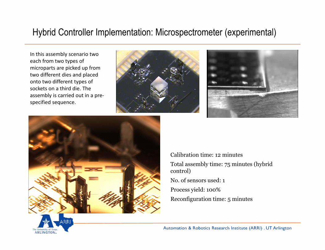
Hybrid Controller Implementation: Microspectrometer (experimental)

In this assembly scenario two each from two types of microparts are picked up from two different dies and placed onto two different types of sockets on a third die. The assembly is carried out in a pre‐specified sequence.

Calibration time: 12 minutes

Total assembly time: 75 minutes (hybrid control)control)

No. of sensors used: 1

Process yield: 100%

Reconfiguration time: 5 minutes

Conclusion

Automated, deterministic serial microassembly provides a pathway to build high yield and cost effective complex heterogeneous microsystems.

A major drawback of closed loop serial microassembly is low speed and space constraints inA major drawback of closed loop serial microassembly is low speed, and space constraints in sensing.

Precision measures for robotic system are redefined to associate resolution with visual servoing, repeatability with calibrated operation, and accuracy with open loop operation.g p y p y p p p

The High Yield Assembly Condition (HYAC) guarantees nearly 100% assembly yield of compliant MEMS. This condition is the basis for controller selection using RRA rules.

By implementing a hybrid controller which selects suitable assembly control based on theBy implementing a hybrid controller which selects suitable assembly control based on the precision requirements of a specific task in the sequence, additional objectives, such as low cycle time can be accomplished.

We presented a virtual 3D microassembly environment having necessary and sufficient visual, kinematic dynamic realism in order to test multiple assembly schemes prior to assembly.

We demonstrated assemblies of complex microsystems such as the microspectrometer showing that the hybrid controller is more efficient than pure open loop, or pure closed loop control.

Thank you!

Contact: www.arri.uta.edu/popa, [email protected]

Building microsouvenir “Microtemple of Zeus”

Acknowledgement: US Office of Naval Research, grants #N00014‐05‐1‐0587, 000 06 0 d 000 08 C 0390#N00014‐06‐1‐1150, and #N00014‐08‐C‐0390.

Documents

Precision-Driven Hybrid Control for 3D Microassembly