PRECISE LOCAL GEOID DEFINITION CASE STUDY: NISYROS … · 2018-05-26 · leveling). It provides global geoid estimation of the order of ±5 to ±10 cm over areas covered with high

International Journal of Engineering Technology and Scientific Innovation

ISSN: 2456-1851

Volume:03, Issue:02 "March-April 2018"

www.ijetsi.org Copyright © IJETSI 2018, All right reserved Page 107

PRECISE LOCAL GEOID DEFINITION CASE STUDY:

NISYROS ISLAND IN GREECE

Evangelia Lambrou

Laboratory of General Geodesy, School of Rural and Surveying Engineering,

National Technical University of Athens, 15780, Greece

ABSTRACT

The global geoid model EGM08 consists nowadays one of the best tools for quick transformation

of geometric heights which provided by GNSS measurements to orthometric ones. Nevertheless

there are some areas worldwide, where the adaptation of EGM08 is not satisfactory due to large

terrain fluctuations (high mountains, spread islands etc.) or due to strong gravity anomalies.

Moreover, the unification of vertical datums between the islands and mainland in Greece as well

as between adjacent countries remains a main goal which is mainly supported by satellite gravity

missions, e.g., the CHAMP, GRACE and GOCE satellites in order to produce accurate and

reliable GGMs.

Thus, the determination of accurate (under cm) orthometric heights via the geometric ones is

required by the demanding infrastructure and monitoring projects.

It is well known that geometric heights are easily obtained by GNSS measurements, while the

orthometric ones are extremely demanding in time and staff in order to be determined by some

mm accuracy.

This study applies a simultaneous measurement project of orthometric and geometric height

differences in order to assess in terms of time and cost, the calculation of a precise (under cm)

local geoid on Nisyros island- Greece.

Nisyros Island is located at the southeast edge of the Aegean Sea. A 13 benchmarks (BMs)

network was properly spread on the island. GNSS measurements were carried out by the relative

static positioning method. The orthometric height differences between BMs were measured by

the method of Accurate Trigonometric Heighting. The orthometric and geometric height of each

benchmark (BM) was determined with ±6mm and ±10mm respectively by applying least square

adjustments. The best adaptation equation is determined for the local geoid undulation.

Additionally the corresponding values of the geoid undulation N were calculated by the EGM08


ISSN: 2456-1851



as well as a reduction equation. Moreover the zero-level geopotential value (Wo) of the island,

has been determined and be compared to the corresponding ones of the neighboring to Nisyros

Hellenic islands and the Greek Vertical Datum (GVD).

Keywords: local geoid model, Accurate Trigonometric Heighting, reduction equation for

EGM08, Local Vertical Datum, zero-level geopotential value, Nisyros Island

I. INTRODUCTION

The Global positioning system provides

ellipsoidal (geometric) heights, which have

no physical meaning. For this reason they

aren’t used in engineering and infrastructure

applications. Thus the main request of the

geodetic community is the accurate

transformation of the acquired geometric

heights to orthometric ones. The Global

geoid model EGM08 contributes a lot to this

effort as includes enormous quantity of

several kinds of data (altimetry, gravimetric,

leveling). It provides global geoid estimation

of the order of ±5 to ±10 cm over areas

covered with high quality of gravity data.

The model includes gravity anomalies

according to a global 5 arc-minute grid and

reaches spherical harmonic degree of order

2159 which corresponds to a grid size of

approximately 7km on the earth surface

[1],[2],[3].

Also reliable geoid models may be derived

nowadays from gravity data obtained from

satellite gravity missions, e.g., the CHAMP,

GRACE and GOCE satellites. These GGMs

provide adequate accuracies for a large

number of geodetic applications [4],

[5].Additionally, GOCE data support the

determination of the zero-level geopotential

value towards the unification of Local

Vertical Datums (LVD) to a global one. [6],

[7]

However in some areas, where there is lack

of data or large scale topographic

discontinuities, large discrepancies of half a

meter or more are noticed [8]. Also for small

areas under the resolution of the EGM08 the

provided data may be unreliable. In these

cases the comparison of a well fitted local

model with the global ones may give useful

information for the examined area and the

opportunity to use the EGM08 or GGMs by

following the calculated reduction equation.

The successfulness of the scientific

researches is to determine geoid heights at

cm level as this is required by the modern

infrastructure and constructions

[9],[10],[11],[12],[13],[14],[15].

A well–known method for the calculation of

the local geoids model, which is also used

for the evaluation of the above mentioned

global models, is the GPS/leveling data

processing. This demands both geometric

and orthometric heights at adequate number

of control points at the interest area in order

to calculate satisfactory local geoid heights

by sub centimeter accuracy. This

presupposes to obtain both the geometric


ISSN: 2456-1851



and orthometric heights of the control points

with some mm accuracy. Thus the geoid

heights as well as their uncertainties are

calculated by using the well known

equations 1.

iii h-H N and 2

h

2

HN iiiσσσ (1)

In practice, this procedure is the

approximation by using measured GNSS

and leveling height differences. So the geoid

heights N are used for a model creation in

the interest area. The geodetic coordinates (

φ , λ ) or the local plan coordinates (x, y)

are used for the adjustment[16].

Many researches have been carried out on

the local geoid determination by using

conventional, modern and artificial neural

networks methods [17], [18], [19], [20],

[21], [15]. Well known techniques as the

bilinear interpolation, polynomial

regression, triangulation, nearest-neighbor

interpolation [22], [8] and Artificial Neural

networks (ANNs) have recently be used for

this purpose with success [23], [24], [25],

[26]. The method to be used for the

modeling depends on the number of control

points, the degree of freedom and the size of

the area as far as the statistical tests are

satisfied [27], [28], [29].

In the aforementioned works usually the

used geometric height differences come out

by direct GNSS measurements between the

BMs as the orthometric ones, due to the

difficulty in their acquisition, are provided

by different time period campaigns. Usually

they are of less accuracy and reliability.

The aim of this work is to investigate the

possibility, the time and the cost needed in

order to perform a simultaneous orthometric

and geometric height differences

measurement project for the determination

of sub centimeter local geoid.

II. THE STUDY AREA AND THE DATA

ACQUISITION

Nisyros Island is located at the southeast

edge of the Aegean Sea (figure 1a) covering

an area of 41Km2. It has almost round shape,

with radius 3.6Km. Nisyros was created by

the volcano eruptions, which is situated

almost at its center.

Figure 1a: The Nisyros’ Island

A network of 13 BMs was established

(figure 1b), on the island. The benchmarks

are distributed at a grid of 1km to 4Km in


ISSN: 2456-1851



order to cover the examined area. Special

attention was paid for their accessibility.

Twenty eight connections were formed

between them.

Thus for the geometric heights acquisition

28 baselines of 1.5km to 6Km were

measured by using the GNSS static

positioning method. Two Trimble 5800

double frequency GNSS receivers are used

[30].

Figure 1b: The geodetic network

The occupation time for each baseline

ranges between 1 to 1.5 hours. The net time

for the GNSS measurements was about 40

hours as the total needed time including the

transportations of the instrumentation is

about 5 days, by a crew of at least two

persons.

The 28 orthometric height differences (ΔH)

between the same BMs were measured by

using the accurate trigonometric heighting

method [31], [32]. This method uses the

trigonometric leveling method by

simultaneous and reciprocal observations of

zenith angles and distances between the

points. Thus the error of the refraction is

eliminated and also the instrument and target

heights aren’t needed. The use of this

method for height difference measurement

ensures errors of some mm for distances up

to 5 Km. The total stations Leica TCR1201+

and TM30 are used which provide ±1’’and

±0.5’’angle accuracy respectively and

±1mm distance measurement accuracy [33],

[34]. The time needed for each height

difference measurement ranges between 1 to

3 hours. This depends on the distance

between the points, the total number of the

intermediate instrument stations and the

time for the instrumentation transportation.

The total time for the network measurement

reaches 10 days, by a crew of at least three

persons.

III. DATA PROCESSING

The BM T1 which is a cement pillar of the

Hellenic Military Geographic Service

(HMGS), was decided to be the fix point of

the network. So the orthometric height of

T1 is provided by the national network

adjustment[35]. The geometric height of T1

is provided, relative to the GRS80 ellipsoid,

by the Hellenic positionig system HEPOS,

when a six month campain was carried out

on 2007 in order to determine reliable GNSS

measurements and coordinates for 2470

stations in Greece for the system

completion[36].


ISSN: 2456-1851



The appropriate reductions are implemended

to both T1 heights for their transformation

to the zero-tide system in order to be

compatible with the Local Verical Datum

(LVD) calculation which will follow. For

the geometric height the reduction [37], [38]

is given by the equation 2

ZT FT 2h h (0.099 0.296 sin φ) (2)

where = 0.62 and hFT and hZT are the

geometric height of the tide free and zero-

tide reference ellipsoid. This negative

correction equals to – 4 mm .

Moreover the orthometric height is referred

to measurements implemented by the

HMGS in Greece where no tidal corrections

were performed [39] thus the equation 3 is

used

ZT MT 2H H (0.099 0.296 sin φ) (3)

where HZT and HMT are the orthometric

heights of the zero-tide geoid and the mean

tide geoid respectively. This negative

correction equals to -6mm.

Separate least square adjustment was

applied for each network (orthometric and

geometric) with 12 unknown heights and 16

degrees of freedom. Thus the orthometric

and geometric heights of each benchmark

are determined with uncertainties, which

range between 3mm to 6mm and 6mm

to 10 mm respectively.

Also by using the formulaijijij Δh-ΔH ΔN , the

28 geoid undulation differences are

calculated and the undulation N at each BM

is determined by another least square

adjustment with σ0 = 11mm. The geoid

undulations Ni range between 30.01m to

30.50m.

Table 1 summarizes the results. In figure 2

the N/S (2a) and the W/E (2b) profiles of the

geoid undulation are presented, while the

contours of the geoid undulation N are

drawn by 5cm interval (figure 3).It is

obvious that there is a regular tilt of the

geoid surface towards the ellipsoid from S/E

to N/W equal to 0.07‰.

(a)

(b)

30.000

30.100

30.200

30.300

30.400

30.500

30.600

36.55 36.56 36.57 36.58 36.59 36.6 36.61 36.62 36.63

Latitude φ (o)

N (

GP

S/

Levell

ing

) (m

)

30.000

30.100

30.200

30.300

30.400

30.500

30.600

27.12 27.13 27.14 27.15 27.16 27.17 27.18 27.19 27.2 27.21

Longitude λ (o)

Ν (

GP

S/

Levell

ing

) (m

)


ISSN: 2456-1851



Figure 2: The profile of the geoid undulation N/S (2a) and W/E (2b)

Table 1: The positions of the benchmarks and the adjustments results

point φ λ Η

(m)

h

(m)

Ν

(m)

T1 36°.62067262 27°.16857822 27.987 58.443 30.456

T2 36°.61470111 27°.13980346 2.123 32.623 30.500

G1 36°.61319996 27°.15322208 3.239 33.704 30.465

G2 36°.60193776 27°.15182674 259.919 290.342 30.423

G3 36°.59729204 27°.20420953 3.173 33.349 30.175

G4 36°.57876786 27°.16688977 112.615 142.835 30.220

G5 36°.58912929 27°.19411270 277.099 307.265 30.166

G6 36°.56817932 27°.18635222 273.709 303.750 30.041

G7 36°.55906276 27°.17591012 33.808 63.822 30.015

G8 36°.57710666 27°.14853694 280.835 311.141 30.306

G9 36°.59150701 27°.13803597 252.468 282.886 30.418

KASTRO 36°.60615829 27°.13030798 112.374 142.887 30.513

3010 36°.60517342 27°.16971229 453.807 484.182 30.375

Mean uncertainty ±6mm ±10mm ±11mm

Figure 3: The Nisyros’ geoid contours by 5cm interval


ISSN: 2456-1851



IV. PARAMETRIC APPROXIMATION

MODELS

Polynomial regression method was applied

in order to express the geoid surface via an

adaptation equation, as the examined area is

small. First and second degree equations

were tried. The following equation 4

presents a Simple Planar Surface with

RMSE 2.3 cm, as the equation 5 presents a

better approximation by second degree

polynomial with RMSE 0.4 cm.

Where φ0, λ0 (rad) are the mean values of

latitude and longitude correspondingly

Figure 4 illustrates the geoid surface

modeling by using Simple Planar Surface

(left) and Quadratic Surface (right).

Figure 4: The Geoid surface modeling by

Simple Planar (left) and Quadratic

Surface (right)

V. A REDUCTION EQUATION OF

NEGM08

As it is referred above Nisyros is a limited

almost round area of about 4Km radius. The

resolution of EGM08 reaches the 8Km. So,

there is a little likelihood to derive reliable

NEGM08 values for the BMs. Nevertheless in

order to exploit the capability of EGM08 it

was decided to carry out the procedure and

also to attempt the determination of a

reduction equation in order to correct the

provided NEGM08.

The geometric heights of the BMs are

calculated in the zero-tide system according

to the EGM2008 global geopotential model

on the GRS80 reference ellipsoid1 by using

the harmonic_synth_v02 software program

that is freely provided by the NGA/EGM

development team[40].

The zero degree term, No which represents

the difference between the GM-values of the

EGM2008 mean ellipsoid and the


ISSN: 2456-1851



correspondent ones of the reference ellipsoid

GRS80 of GPS/ leveling system was also

included. The additive term No is given by

the equation 6 as the contribution of the

zero-degree harmonic to the EGM2008

geoid height with respect to the GRS80

ellipsoid [41].

γ

UW-

γR

MGGM(m)N 00

0

(6)

where

GM and Uo represents the Somigliana -

Pizzeti normal gravity field referred to the

GRS80 ellipsoid (GM = 398600.50 × 109

m3/s2 and Uo =62636860.85m2/s2).

The Earth’s geocentric gravitational constant

GM = 398600.4415 × 109 m3/s2 and the

geoidal gravity potential equals to Wo

=62636856.00m2/s2.

The value R = 6371008.771m was set for

the mean Earth radius according to GRS80

and finally the normal gravity γ on the

reference ellipsoid was computed at each

point from Somigliana’s formula.

According to the above mentioned values

the zero-degree term No is incorporated to

the computations equal to -0.422m for all

the BMs due to the limited area of the

island. Table 2 presents the NEGM08 as well

as the differences ΔΝ between N GPS/LEV and

NEGM08, which range between -50cm to -

58cm with mean value of -0.531m±24mm.

In figure 5 the profile of the differences ΔΝ

towards N/S and W/E is illustrated.

Figure 5: The profile of the differences

ΔΝ towards N/S and W/E


ISSN: 2456-1851



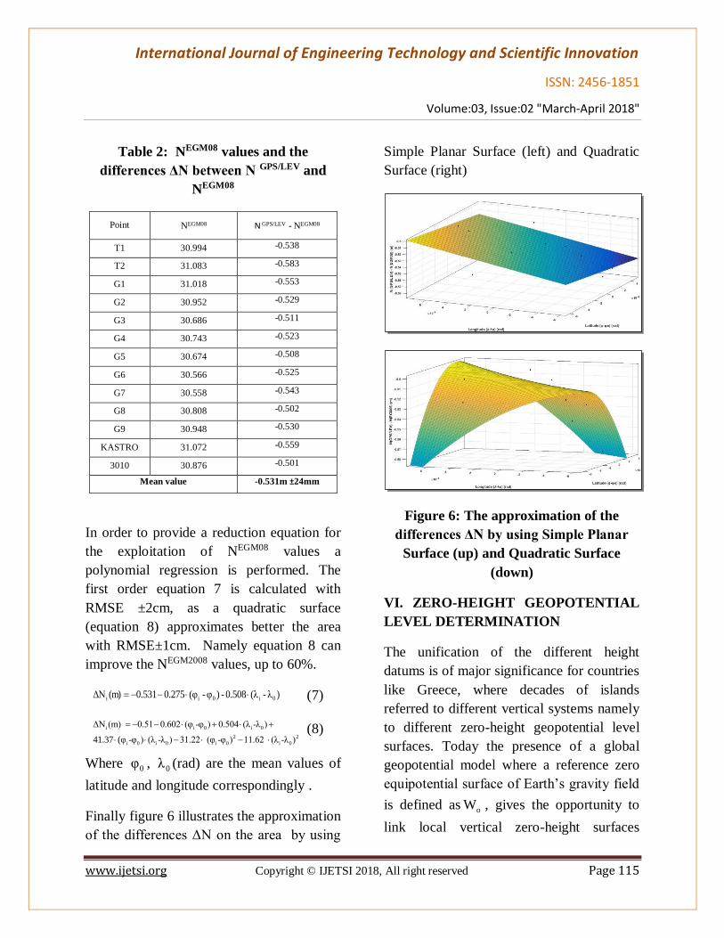
Table 2: NEGM08 values and the

differences ΔΝ between N GPS/LEV and

NEGM08

Point NEGM08 Ν GPS/LEV - NEGM08

T1 30.994 -0.538

T2 31.083 -0.583

G1 31.018 -0.553

G2 30.952 -0.529

G3 30.686 -0.511

G4 30.743 -0.523

G5 30.674 -0.508

G6 30.566 -0.525

G7 30.558 -0.543

G8 30.808 -0.502

G9 30.948 -0.530

KASTRO 31.072 -0.559

3010 30.876 -0.501

Mean value -0.531m ±24mm

In order to provide a reduction equation for

the exploitation of NEGM08 values a

polynomial regression is performed. The

first order equation 7 is calculated with

RMSE ±2cm, as a quadratic surface

(equation 8) approximates better the area

with RMSE±1cm. Namely equation 8 can

improve the NEGM2008 values, up to 60%.

)λ-(λ.5080-)φ-(φ 275.0531.0(m)ΔN 0i0ii (7)

i i 0 i 0

2 2

i 0 i 0 i 0 i 0

ΔN (m) 0.51 0.602 (φ -φ ) 0.504 (λ -λ )

41.37 (φ -φ ) (λ -λ ) 31.22 (φ -φ ) 11.62 (λ -λ )

(8)

Where 0φ , 0λ (rad) are the mean values of

latitude and longitude correspondingly .

Finally figure 6 illustrates the approximation

of the differences ΔΝ on the area by using

Simple Planar Surface (left) and Quadratic

Surface (right)

Figure 6: The approximation of the

differences ΔΝ by using Simple Planar

Surface (up) and Quadratic Surface

(down)

VI. ZERO-HEIGHT GEOPOTENTIAL

LEVEL DETERMINATION

The unification of the different height

datums is of major significance for countries

like Greece, where decades of islands

referred to different vertical systems namely

to different zero-height geopotential level

surfaces. Today the presence of a global

geopotential model where a reference zero

equipotential surface of Earth’s gravity field

is defined as oW , gives the opportunity to

link local vertical zero-height surfaces


ISSN: 2456-1851



LVD

oW ,by calculated their differences from

the global oW .

Various methods have been used for the

estimation of the fundamental parameterLVD

oW , which can be broadly classified into

two basic categories described by Kotsakis

et al. (2010). The first one is based on the

combined adjustment of GGM and

GPS/leveling data [42], [43], while the other

uses the formulation of a geodetic boundary

value problem with the use of gravity

anomaly data over different LVD zones

[44], [45], [46], [47]. According to the first

method LVD

oW of the Local Vertical Datum

was computed using the equation 9 [42],

[48]:

m

gNHhWW

i

m

1 iii

o

LVD

o

(9)

where

oW = 62 636 856.0 m2/s-2

hi = the geometric height of each BM

derived by GNSS measurements

Hi = the orthometric height of each BM

Ni =the geoid height derived from GGMs

gi =the gravity at each BM computed from

GGMs and

m = the total number of the available BMs

i.e 13 in this case.

Three parametric models have been tested

according to Kotsakis et al. 2012. The first

one is the null model, where no systematic

errors or biases are modeled. The second

one, where systematic differences are

modeled in terms of a scaling factor and the

third one, where the tilt between the two

reference surfaces, the geoid and the

ellipsoid, is represented by the tilt

components x1 for N/S and x2 for the W/E.

Table 3 illustrates the results. The LVD

oW

which came out by the three models are

close to each other while the first model

provides the smaller RMSE 4cm.

Table 3: The estimated LVD

oW for Nisyros

by using three different parametric

models.

Model

xaT

i )/s(m

W

22

LVD

o

)/s(m

W-W

22

o

LVD

o

(cm)

δHLVD

o

0 62636861.20

0.04 5.20 0.04 -53.1 4

iHδs 62636861.37

0.07 5.37 0.07 -54.8 7

i0i20i1 φcos)λ-(λx)φφ(x 62636861.21

0.06 5.21 0.06 -53.2 6

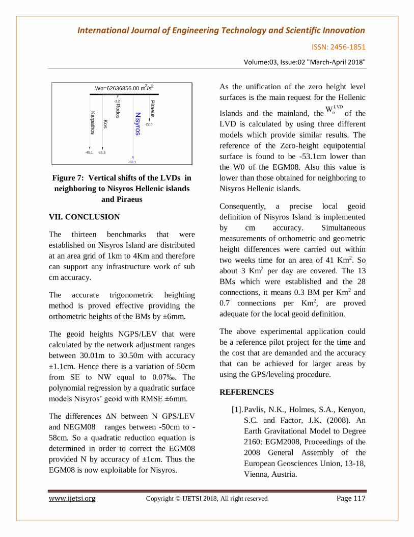
Finally figure 7 illustrates the vertical shifts

in (cm) of the LVDs in three neighboring

Hellenic islands and the mainland (Piraeus)

relative to the conventional global reference

value Wo as they have been calculated by

Kotsakis et al 2012.

http://www.sciencedirect.com/science/article/pii/S1674984716301495#bib10


ISSN: 2456-1851



Wo=62636856.00 m /s2 2

Ka

rpa

thos

Ko

s

Ro

dos

Nis

yro

s

Pira

eu

s

-45.1 -45.3

-3.2

-53.1

-22.0

Figure 7: Vertical shifts of the LVDs in

neighboring to Nisyros Hellenic islands

and Piraeus

VII. CONCLUSION

The thirteen benchmarks that were

established on Nisyros Island are distributed

at an area grid of 1km to 4Km and therefore

can support any infrastructure work of sub

cm accuracy.

The accurate trigonometric heighting

method is proved effective providing the

orthometric heights of the BMs by ±6mm.

The geoid heights NGPS/LEV that were

calculated by the network adjustment ranges

between 30.01m to 30.50m with accuracy

±1.1cm. Hence there is a variation of 50cm

from SE to NW equal to 0.07‰. The

polynomial regression by a quadratic surface

models Nisyros’ geoid with RMSE ±6mm.

The differences ΔΝ between N GPS/LEV

and NEGM08 ranges between -50cm to -

58cm. So a quadratic reduction equation is

determined in order to correct the EGM08

provided N by accuracy of ±1cm. Thus the

EGM08 is now exploitable for Nisyros.

As the unification of the zero height level

surfaces is the main request for the Hellenic

Islands and the mainland, theLVD

oWof the

LVD is calculated by using three different

models which provide similar results. The

reference of the Zero-height equipotential

surface is found to be -53.1cm lower than

the W0 of the EGM08. Also this value is

lower than those obtained for neighboring to

Nisyros Hellenic islands.

Consequently, a precise local geoid

definition of Nisyros Island is implemented

by cm accuracy. Simultaneous

measurements of orthometric and geometric

height differences were carried out within

two weeks time for an area of 41 Km2. So

about 3 Km2 per day are covered. The 13

BMs which were established and the 28

connections, it means 0.3 BM per Km2 and

0.7 connections per Km2, are proved

adequate for the local geoid definition.

The above experimental application could

be a reference pilot project for the time and

the cost that are demanded and the accuracy

that can be achieved for larger areas by

using the GPS/leveling procedure.

REFERENCES

[1]. Pavlis, N.K., Holmes, S.A., Kenyon,

S.C. and Factor, J.K. (2008). An

Earth Gravitational Model to Degree

2160: EGM2008, Proceedings of the

2008 General Assembly of the

European Geosciences Union, 13-18,

Vienna, Austria.


ISSN: 2456-1851



[2]. Pavlis, N.K., Holmes, S.A., Kenyon,

S.C. and Factor, J.K. (2012) The

Development and Evaluation

of the Earth Gravitational Model

2008 (EGM2008), Journal of

Geophysical Research: Solid Earth

(1978-2012), 117(B4): 4406.

http://earth-

info.nga.mil/GandG/wgs84/gravitym

od/egm2008/

[3]. Andritsanos VD, Arabatzi O,

Gianniou M, Pagounis V, Tziavos

IN, Vergos GS, Zachris E (2015)

Comparison of Various GPS

Processing Solutions toward an

Efficient Validation of the Hellenic

Vertical Network: The ELEVATION

Project. J Surv Eng, doi:

10.1061/(ASCE)SU.1943-

5428.0000164, 04015007.

[4]. Andritsanos V.D., Grigoriadis V.N.,

Natsiopoulos D.A., Vergos G.S.,

Gruber T., Fecher T. (2017) GOCE

Variance and Covariance

Contribution to Height System

Unification. In: International

Association of Geodesy Symposia.

Springer, Berlin, Heidelberg.

[5]. Vergos G.S., Andritsanos V.D.,

Grigoriadis V.N., Pagounis V.,

Tziavos I.N. (2015) Evaluation of

GOCE/GRACE GGMs Over Attica

and Thessaloniki, Greece, and Wo

Determination for Height System

Unification. In: Jin S., Barzaghi R.

(eds) IGFS 2014. International

Association of Geodesy Symposia,

vol 144. Springer, Cham.

[6]. Vergos, G.S., Erol, B., Natsiopoulos,

D.A. Preliminary results of GOCE-

based height system unification

between Greece and Turkey over

marine and land areas Acta Geod

Geophys (2018) 53: 61.

https://doi.org/10.1007/s40328-017-

0204-x.

[7]. Soycan M. (2013) Analysis of

geostatistical surface model for gps

height transformation: a case study

in Izmir territory of

Turkey.702Geodetski vestnik 57/4.

[8]. Vanicek, P., and A. Kleusberg

(1987). The Canadian geoid—

Stokesian approach. Manuscripta

Geodaetica 12, 86-98.

[9]. Li Y. C., Sideris M.G. (1994).

Minimization and estimation of

geoid undulation errors. Bulletin

Geodesique 68:201-219

[10]. Tóth, Gy., Rózsa, Sz.,

Andritsanos, V.D., Ádám, J.,

Tziavos, I.N., (2000). Towards a

cm–Geoid for Hungary: Recent

Efforts and Results. Phys. Chem.

Earth (A), 25:1:47–52

[11]. Kühtreiber N. (2002). High

Precision Geoid Determination of

Austria Using Heterogeneous Data.

International Association of

Geodesy. Section III - Determination

of the Gravity Field. 3rd Meeting of

the International Gravity and Geoid

Commission. Gravity and Geoid

http://earth-info.nga.mil/GandG/wgs84/gravitymod/egm2008/



https://doi.org/10.1007/s40328-017-0204-x

https://doi.org/10.1007/s40328-017-0204-x


ISSN: 2456-1851



2002 - GG2002. ed. I.N. Tziavos

(144-151)

[12]. Chen Y., Luo Z., Kwok S.

(2003). Precise Hong Kong Geoid

HKGEOID-2000. Journal of

Geospatial Engineering, Vol. 5, No.

2, pp. 35-41.

[13]. Soycan, M., (2006).

Determination of Geoid Heights by

GPS and Precise Trigonometric

Levelling. Survey Review 38-299,

387-396.

[14]. Abbak R.A., Sjöberg L.E.,

Ellmann A., Ustun A. (2012). A

precise gravimetric geoid model in a

mountainous area withscarce gravity

data: a case study in central Turkey.

Studia Geophysica et Geodaetica.

56- 4, 909-927.

[15]. Ollikainen M. (1997).

Determination Of Orthometric

Heights Using GPS Levelling

Publications of the Finnish Geodetic

Institute’ KirkkonummI.

[16]. Kiamehr, R. and Sjoberg,

L.E. (2005). Comparison of the

qualities of recent global and local

gravimetric geoid model in Iran.

Studia Geophysica et Geodaetica,

49: 289-304.

[17]. Benahmed Dahoa, S.A.,

Kahlouchea, S., Fairhead, J.D.

(2006). A procedure for modeling

the differences between the

gravimetric geoid model and

GPS/leveling data with an example

in the north part of Algeria.

Computers & Geosciences 32, 1733–

1745.

[18]. Featherstone, W. E., Sproule,

D. M. (2006). Fitting Ausgeoid98 to

the Australian height datum using

GPS-leveling and least squares

collocation: application of a cross-

validation technique. Survey Review

38-301, 574-582.

[19]. Kotsakis, C., Katsambalos,

K. (2010). Quality analysis of global

geopotential models at 1542

GPS/leveling benchmarks over the

Hellenic mainland. Survey Review

42-318, 327-344.

[20]. Erol, B., Erol, S., Çelik, R. N.

(2008). Height transformation using

regional geoids and GPS/leveling in

Turkey, Survey Review, 40-307, 2-

18.

[21]. Soycan, M., Soycan A.,

(2003). Surface Modeling for GPS-

Leveling Geoid Determination.

International Geoid Service 1-1, 41-

51.

[22]. Stopar B, Ambrozic T, Kuhar

M, Turk G (2000). Artificial neural

network collocation method for local

geoid height determination.Proc IAG

Int Sym Gravity, Geoid and

Geodynamics 2000, Banff, Canada,

CD-Rom

[23]. Kavzoglu T, Saka MH

(2005). Modelling Local

GPS/Levelling Geoid Undulations

Using Artificial Neural Networks, J.

Geodesy, 78: 520-527.


ISSN: 2456-1851



[24]. Kuhar M., Stopar B., Turk

G., Ambrozÿicÿ T. (2001). The use

of artificial neural network in geoid

surface approximation. AVN 2001,

pp. 22-27.

[25]. Kutoglu HS (2006). Artificial

neural networks versus surface

polynomials for determination of

local geoid, 1st International Gravity

Symposium, Istanbul.

[26]. Kraus K. and Mikhail E.M.

(1972). Linear Least-Squares

Interpolation 12. Congress of the

International Society of

Photogrammetry, Ottawa, Canada,

July 23-August 5.

[27]. Miller C.L. and Laflamme R.

A. (1958). The Digital Terrain

Model Theory and Application,

Presented at the Society’s 24. Annual

Meeting, Hotel Shoreham,

Washington, D.C March 27.

[28]. Schut G.H. (1976). Review

of Interpolation Methods for Digital

Terrain Models. The Canadian

Surveyor, Vol. 30. No. 5,

[29]. https://www.positioningsoluti

ons.com/Trimble/product_specs/580

0specs.pdf

[30]. Lambrou E. (2007) Accurate

height difference determination

using reflect or less total stations (in

Greek). Technika Chronika Sci J

Tech Chamber Greece 1–2:37–46

[31]. Lambrou E, Pantazis G.

(2007). A convenient method for

accurate height differences

determination. In: Proceedings of the

17th International Symposium on

Modern technologies, education and

professional practice in Geodesy and

related fields, Sofia, pp 45–53

[32]. http://www.toposurvey.ro/sec

undare/Leica/Leica_TPS1200+_Tec

hnicalData_en.pdf

[33]. http://surveyequipment.com/a

ssets/index/download/id/220/

[34]. Takos I. (1989). New

adjustment of the national geodetic

networks in Greece (in Greek). Bull

Hellenic Mil Geogr Serv

49(136):19–93.

[35]. Gianniou, M. (2009).

National Report of Greece to

EUREF 2009, EUREF 2009

Symposium, May 27-30 2009,

Florence, Italy.

[36]. Ekman M (1989) Impacts of

geodynamic phenomena on systems

for height and gravity. Bull Geod

63:281–296

[37]. Mäkinen J, Ihde J (2009).

The permanent tide in height

systems. IAG Symp Series, vol 133.

Springer, Berlin 81–87

[38]. Antonopoulos A. (1999)

Models of height systems of

reference and their applications to

the Hellenic area (in Greek). PhD

Thesis, School of Rural and

Surveying Engineering, National

Technical University of Athens,

Greece.

https://www.positioningsolutions.com/Trimble/product_specs/5800specs.pdf



http://www.toposurvey.ro/secundare/Leica/Leica_TPS1200+_TechnicalData_en.pdf



http://surveyequipment.com/assets/index/download/id/220/

http://surveyequipment.com/assets/index/download/id/220/


ISSN: 2456-1851



[39]. Holmes SA, Pavlis NK

(2006). A Fortran program for very-

high degree harmonic synthesis

(version 05/01/2006). Program

manual and software code available

at

[40]. http://earth-

info.nima.mil/GandG/wgs84/gravity

mod/egm2008/

[41]. Heiskanen W, Moritz H

(1967) Physical geodesy. WH

Freeman, San Francisco

[42]. Grigoriadis V.N , Kotsakis

C., Tziavos I.N. (2014). Estimation

of the Reference Geopotential Value

for the Local Vertical Datum of

Continental Greece Using EGM08

and GPS/Leveling Data, 35(1),

International Association of Geodesy

Symposia, pp. 88-89

[43]. Tocho C., Vergos G.S

(2015). Estimation of the

geopotential value W0, for the local

vertical datum of Argentina using

EGM2008 and GPS/levelling data

W0LVD J Biomed Sci, 8 (5), pp. 395-

405

[44]. Amjadiparvar B., Rangelova

E., Sideris M.G. (2016). The GBVP

approach for vertical datum

unification: recent results in North

America J Geodesy, 90 (1), pp. 45-

63

[45]. Gerlach C., Rummel R.

(2013). Global height system

unification with GOCE: a simulation

study on the indirect bias term in the

GBVP approach J Geodesy, 87 (1),

pp. 57-67

[46]. Rummel R., Teunissen P.

(1988). Height datum definition,

height datum connection and the role

of the geodetic boundary value

problem J Geodesy, 62 (4), pp. 477-

498

[47]. Rangelova E., Sideris M.G,

Amjadiparvar B. et al (2015). Height

datum unification by means of the

GBVP approach using tide gauges

VIII Hotine-Marussi Symposium on

Mathematical Geodesy, 142,

Springer International Publishing,

pp. 121-129.

[48]. Kotsakis, C., Katsambalos,

K., Abatzidis D. (2012). Estimation

of the zero-height geopotential level

W0LVD in a local vertical datum from

inversion of co-located GPS,

leveling and geoid heights: a case

study in the Hellenic islands,

J Geodesy, 86 (6), pp. 423-439

http://earth-info.nima.mil/GandG/wgs84/gravitymod/egm2008/



Documents

PRECISE LOCAL GEOID DEFINITION CASE STUDY: NISYROS … · 2018-05-26 · leveling). It provides global geoid estimation of the order of ±5 to ±10 cm over areas covered with high