Practical Process Control For Engineers and Technicians · Presents Practical Process Control For Engineers and Technicians Revision 9 Website: E-mail: [email protected]

Practical Process Control For Engineers and Technicians

WHO ARE WE? IDC Technologies is internationally acknowledged as the premier provider of practical, technical training for engineers and technicians. We specialize in the fields of electrical systems, industrial data communications, telecommunications, automation and control, mechanical engineering, chemical and civil engineering, and are continually adding to our portfolio of over 60 different workshops. Our instructors are highly respected in their fields of expertise and in the last ten years have trained over 200,000 engineers, scientists and technicians. With offices conveniently located worldwide, IDC Technologies has an enthusiastic team of professional engineers, technicians and support staff who are committed to providing the highest level of training and consultancy. TECHNICAL WORKSHOPS TRAINING THAT WORKS We deliver engineering and technology training that will maximize your business goals. In today’s competitive environment, you require training that will help you and your organization to achieve its goals and produce a large return on investment. With our ‘training that works’ objective you and your organization will:

• Get job-related skills that you need to achieve your business goals • Improve the operation and design of your equipment and plant • Improve your troubleshooting abilities • Sharpen your competitive edge • Boost morale and retain valuable staff • Save time and money

EXPERT INSTRUCTORS We search the world for good quality instructors who have three outstanding attributes:

1. Expert knowledge and experience – of the course topic 2. Superb training abilities – to ensure the know-how is transferred effectively and quickly to you in

a practical, hands-on way 3. Listening skills – they listen carefully to the needs of the participants and want to ensure that you

benefit from the experience. Each and every instructor is evaluated by the delegates and we assess the presentation after every class to ensure that the instructor stays on track in presenting outstanding courses. HANDS-ON APPROACH TO TRAINING All IDC Technologies workshops include practical, hands-on sessions where the delegates are given the opportunity to apply in practice the theory they have learnt. REFERENCE MATERIALS A fully illustrated workshop book with hundreds of pages of tables, charts, figures and handy hints, plus considerable reference material is provided FREE of charge to each delegate. ACCREDITATION AND CONTINUING EDUCATION Satisfactory completion of all IDC workshops satisfies the requirements of the International Association for Continuing Education and Training for the award of 1.4 Continuing Education Units. IDC workshops also satisfy criteria for Continuing Professional Development according to the requirements of the Institution of Electrical Engineers and Institution of Measurement and Control in the UK, Institution of Engineers in Australia, Institution of Engineers New Zealand, and others.

THIS BOOK WAS DEVELOPED BY IDC TECHNOLOGIES

CERTIFICATE OF ATTENDANCE Each delegate receives a Certificate of Attendance documenting their experience. 100% MONEY BACK GUARANTEE IDC Technologies’ engineers have put considerable time and experience into ensuring that you gain maximum value from each workshop. If by lunchtime on the first day you decide that the workshop is not appropriate for your requirements, please let us know so that we can arrange a 100% refund of your fee. ONSITE WORKSHOPS All IDC Technologies Training Workshops are available on an on-site basis, presented at the venue of your choice, saving delegates travel time and expenses, thus providing your company with even greater savings. OFFICE LOCATIONS

AUSTRALIA • CANADA • INDIA • IRELAND • MALAYSIA • NEW ZEALAND • POLAND • SINGAPORE • SOUTH AFRICA • UNITED KINGDOM • UNITED STATES

[email protected] www.idc-online.com

Visit our website for FREE Pocket Guides IDC Technologies produce a set of 6 Pocket Guides used by

thousands of engineers and technicians worldwide. Vol. 1 – ELECTRONICS Vol. 4 – INSTRUMENTATION Vol. 2 – ELECTRICAL Vol. 5 – FORMULAE & CONVERSIONS Vol. 3 – COMMUNICATIONS Vol. 6 – INDUSTRIAL AUTOMATION

To download a FREE copy of these internationally best selling pocket guides go to:

www.idc-online.com/downloads/

Presents

Practical Process Control

For Engineers and Technicians

Revision 9

Website: www.idc-online.com E-mail: [email protected]

IDC Technologies Pty Ltd PO Box 1093, West Perth, Western Australia 6872 Offices in Australia, New Zealand, Singapore, United Kingdom, Ireland, Malaysia, Poland, United States of America, Canada, South Africa and India Copyright © IDC Technologies 2008. All rights reserved. First published 2008 All rights to this publication, associated software and workshop are reserved. No part of this publication may be reproduced, stored in a retrieval system or transmitted in any form or by any means electronic, mechanical, photocopying, recording or otherwise without the prior written permission of the publisher. All enquiries should be made to the publisher at the address above.

Disclaimer Whilst all reasonable care has been taken to ensure that the descriptions, opinions, programs, listings, software and diagrams are accurate and workable, IDC Technologies do not accept any legal responsibility or liability to any person, organization or other entity for any direct loss, consequential loss or damage, however caused, that may be suffered as a result of the use of this publication or the associated workshop and software.

In case of any uncertainty, we recommend that you contact IDC Technologies for clarification or assistance.

Trademarks All logos and trademarks belong to, and are copyrighted to, their companies respectively. Acknowledgements IDC Technologies expresses its sincere thanks to all those engineers and technicians on our training workshops who freely made available their expertise in preparing this manual.

Contents 1 Introduction 1

1.1 Objectives 1 1.2 Introduction 1 1.3 Basic definitions and terms used in process control 2 1.4 Process modeling 2 1.5 Process dynamics and time constants 6 1.6 Types or modes of operation of available control systems 15 1.7 Closed loop controller and process gain calculations 17 1.8 Proportional, integral and derivative control modes 17 1.9 An introduction to cascade control 18

2 Process Management and Transducers 21 2.1 Objectives 21 2.2 The definition of transducers and sensors 21 2.3 Listing of common measured variables 21 2.4 The common characteristics of transducers 22 2.5 Sensor dynamics 24 2.6 Selection of sensing devices 24 2.7 Temperature sensors 25 2.8 Pressure transmitters 31 2.9 Flow meters 39 2.10 Level transmitters 45 2.11 The spectrum of user models in measuring transducers 47 2.12 Instrumentation and transducer considerations 48 2.13 Selection criteria and considerations 50 2.14 Introduction to the SMART TRANSMITTER 52

3 Basic Principles of Control Valves and Actuators 55

3.1 Objectives 55 3.2 An overview of eight of the most basic types of control valves 55 3.3 Control valve gain, characteristics, distortion and rangeability 70 3.4 Control valve actuators 74 3.5 Control valve positioners 79 3.6 Valve sizing 79

4 Fundamentals of Control Systems 81

4.1 Objectives 81 4.2 ON-OFF control 81 4.3 Modulating control 82 4.4 Open loop control 83 4.5 Closed control loop 84 4.6 Dead time processes 88 4.7 Process responses 89 4.8 Dead zone 90

5 Stability and Control Modes of Closed Control Loops 91 5.1 Objectives 91 5.2 The industrial process in practice 91 5.3 Dynamic behavior of the feed heater 92 5.4 Major disturbances of the feed heater 93 5.5 Stability 93 5.6 Proportional control 96 5.7 Integral control 99 5.8 Derivative control 102 5.9 Proportional, integral and derivative modes 105 5.10 ISA versus “Allen Bradley” 105 5.11 P I and D relationships and related interactions 105

6 Digital Control Principles 109

6.1 Objectives 109 6.2 Digital vs analog: A revision of their definitions 109 6.3 Action in digital control loops 109 6.4 Identifying functions in the frequency domain 110 6.5 The need for digital control 112 6.6 Scanned calculations 115 6.7 Proportional control 115 6.8 Integral control 115 6.9 Derivative control 116 6.10 Lead function as derivative control 116 6.11 Example of incremental form (Siemens S5 - 100V) 117

7 Real and Ideal PID Controllers 119

7.1 Objectives 119 7.2 Comparative descriptions of real and ideal controllers 119 7.3 Description of the IDEAL or the non-interactive PID controller 119 7.4 Description of the real (Interactive) PID controller 120 7.5 Lead function - Derivative control with filter 121 7.6 Derivative action and effects of noise 122 7.7 Example of the KENT K90 controllers PID algorithms 123

8 Tuning of PID Controllers in Both Open and Closed Loop Control Systems 125

8.1 Objectives 125 8.2 Objectives of tuning 125 8.3 Reaction curve method (Ziegler Nichols) 127 8.4 Ziegler Nichols open loop tuning method (1) 129 8.5 Ziegler-Nichols open loop method (2) using POI 130 8.6 Loop time constant (LTC) method 132 8.7 Hysteresis problems that may be encountered in open loop tuning 134 8.8 Continuous cycling method (Ziegler Nichols) 134 8.9 Damped cycling tuning method 136 8.10 Tuning for no overshoot on start up (Pessen) 140 8.11 Tuning for some overshoot on start up (Pessen) 141 8.12 Summary of important closed loop tuning algorithms 141

8.13 PID equations: Dependent and independent gains 141 9 Process Diagrams 145

9.1 Objectives 145 9.2 Controller output 145 9.3 Multiple controller outputs 146 9.4 Saturation and non-saturation of output limits 147 9.5 Cascade control 148 9.6 Initialization of a cascade system 150 9.7 Equations relating to controller configurations 151 9.8 Application notes on the use of equation types 153 9.9 Tuning of a cascade control loop 154 9.10 Cascade control with multiple secondaries 155

10 Concepts and Applications of Feedforward Control 157

10.1 Objectives 157 10.2 Application and definition of feedforward control 157 10.3 Manual feedforward control 158 10.4 Automatic feedforward control 158 10.5 Examples of feedforward controllers 159 10.6 Time matching as feedforward control 159

11 Combined Feedback and Feedforward Control 163 11.1 Objectives 163 11.2 The feedforward concept 163 11.3 The feedback concept 164 11.4 Combining feedback and feedforward control 164 11.5 Feedback - Feedforward summer 164 11.6 Initialization of a combined feedback and feedforward control system 165 11.7 Tuning aspects 165

12 Long Process Dead-time in Closed Loop Control and the Smith Predictor 167

12.1 Objectives 167 12.2 Process deadtime 167 12.3 An example of process deadtime 168 12.4 The Smith Predictor model 169 12.5 The Smith Predictor in theoretical use 170 12.6 The Smith Predictor in reality 171 12.7 An exercise in deadtime compensation 171

13 Basic Principles of Fuzzy Logic and Neural Networks 173

13.1 Objectives 173 13.2 Introduction to fuzzy logic 173 13.3 What is fuzzy logic? 174 13.4 What does fuzzy logic do? 174 13.5 The rules of fuzzy logic 174 13.6 Fuzzy logic example using 5 rules and patches 176 13.7 The Achilles Heel of fuzzy logic 177 13.8 Neural networks 178

13.9 Neural back-propagation networking 179 13.10 Training a neuron network 181 13.11 Conclusions, and then the next step 182

14 Self-Tuning Intelligent Control and Statistical Process Control 183

14.1 Objectives 183 14.2 Self-tuning controllers 183 14.3 Gain scheduling controller 184 14.4 Implementation requirements for self tuning controllers 185 14.5 Statistical process control 185 14.6 Two ways to improve a production process 186 14.7 Obtaining the information required for SPC 187 14.8 Calculating control limits 192 14.9 The logic behind control charts 194

Appendix A Some Laplace Transform Pairs 197 Appendix B Block Diagram Transformation Theorems 201

Appendix C Getting started with PC-ControLAB 203

Appendix D Practical exercises 209

Quiz review 311

1

Introduction

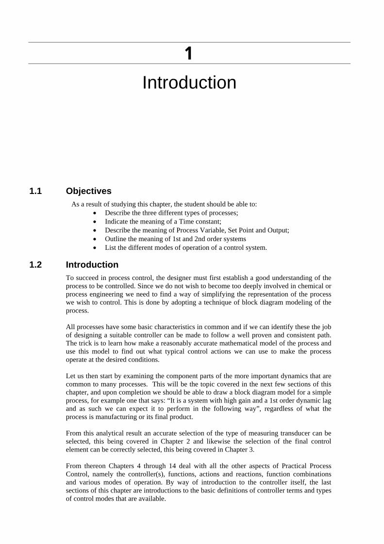
1.1 Objectives As a result of studying this chapter, the student should be able to:

• Describe the three different types of processes; • Indicate the meaning of a Time constant; • Describe the meaning of Process Variable, Set Point and Output; • Outline the meaning of 1st and 2nd order systems • List the different modes of operation of a control system.

1.2 Introduction To succeed in process control, the designer must first establish a good understanding of the process to be controlled. Since we do not wish to become too deeply involved in chemical or process engineering we need to find a way of simplifying the representation of the process we wish to control. This is done by adopting a technique of block diagram modeling of the process. All processes have some basic characteristics in common and if we can identify these the job of designing a suitable controller can be made to follow a well proven and consistent path. The trick is to learn how make a reasonably accurate mathematical model of the process and use this model to find out what typical control actions we can use to make the process operate at the desired conditions. Let us then start by examining the component parts of the more important dynamics that are common to many processes. This will be the topic covered in the next few sections of this chapter, and upon completion we should be able to draw a block diagram model for a simple process, for example one that says: “It is a system with high gain and a 1st order dynamic lag and as such we can expect it to perform in the following way”, regardless of what the process is manufacturing or its final product. From this analytical result an accurate selection of the type of measuring transducer can be selected, this being covered in Chapter 2 and likewise the selection of the final control element can be correctly selected, this being covered in Chapter 3. From thereon Chapters 4 through 14 deal with all the other aspects of Practical Process Control, namely the controller(s), functions, actions and reactions, function combinations and various modes of operation. By way of introduction to the controller itself, the last sections of this chapter are introductions to the basic definitions of controller terms and types of control modes that are available.

2 Practical Process Control

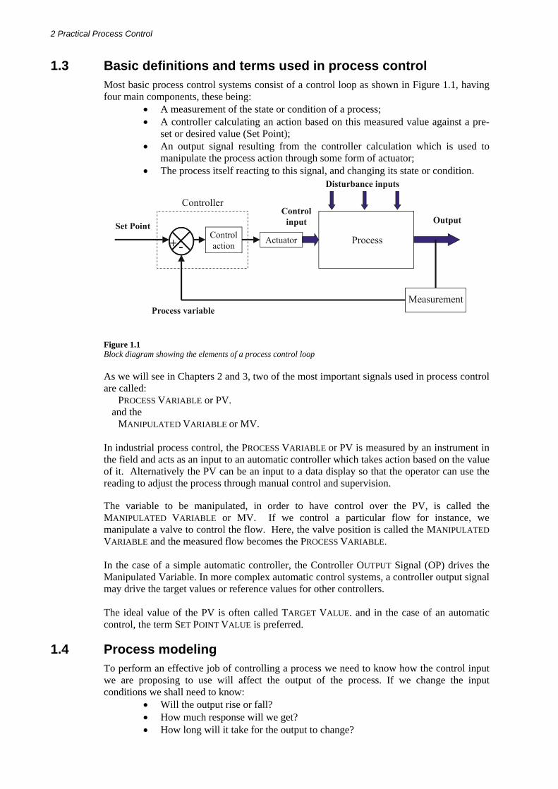
1.3 Basic definitions and terms used in process control Most basic process control systems consist of a control loop as shown in Figure 1.1, having four main components, these being:

• A measurement of the state or condition of a process; • A controller calculating an action based on this measured value against a pre-

set or desired value (Set Point); • An output signal resulting from the controller calculation which is used to

manipulate the process action through some form of actuator; • The process itself reacting to this signal, and changing its state or condition.

Figure 1.1 Block diagram showing the elements of a process control loop

As we will see in Chapters 2 and 3, two of the most important signals used in process control are called:

PROCESS VARIABLE or PV. and the MANIPULATED VARIABLE or MV.

In industrial process control, the PROCESS VARIABLE or PV is measured by an instrument in the field and acts as an input to an automatic controller which takes action based on the value of it. Alternatively the PV can be an input to a data display so that the operator can use the reading to adjust the process through manual control and supervision.

The variable to be manipulated, in order to have control over the PV, is called the MANIPULATED VARIABLE or MV. If we control a particular flow for instance, we manipulate a valve to control the flow. Here, the valve position is called the MANIPULATED VARIABLE and the measured flow becomes the PROCESS VARIABLE. In the case of a simple automatic controller, the Controller OUTPUT Signal (OP) drives the Manipulated Variable. In more complex automatic control systems, a controller output signal may drive the target values or reference values for other controllers. The ideal value of the PV is often called TARGET VALUE. and in the case of an automatic control, the term SET POINT VALUE is preferred.

1.4 Process modeling To perform an effective job of controlling a process we need to know how the control input we are proposing to use will affect the output of the process. If we change the input conditions we shall need to know:

• Will the output rise or fall? • How much response will we get? • How long will it take for the output to change?

Introduction 3

• What will be the response curve or trajectory of the response?

The answers to these questions are best obtained by creating a mathematical model of the relationship between the chosen input and the output of the process in question. Process control designers use a very useful technique of block diagram modeling to assist in the representation of the process and its control system. The following section introduces the principles that we should be able to apply to most practical control loop situations.

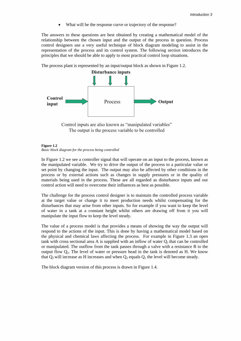
The process plant is represented by an input/output block as shown in Figure 1.2.

Figure 1.2 Basic block diagram for the process being controlled

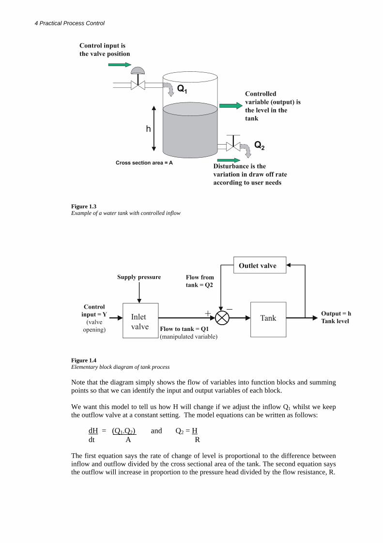
In Figure 1.2 we see a controller signal that will operate on an input to the process, known as the manipulated variable. We try to drive the output of the process to a particular value or set point by changing the input. The output may also be affected by other conditions in the process or by external actions such as changes in supply pressures or in the quality of materials being used in the process. These are all regarded as disturbance inputs and our control action will need to overcome their influences as best as possible. The challenge for the process control designer is to maintain the controlled process variable at the target value or change it to meet production needs whilst compensating for the disturbances that may arise from other inputs. So for example if you want to keep the level of water in a tank at a constant height whilst others are drawing off from it you will manipulate the input flow to keep the level steady. The value of a process model is that provides a means of showing the way the output will respond to the actions of the input. This is done by having a mathematical model based on the physical and chemical laws affecting the process. For example in Figure 1.3 an open tank with cross sectional area A is supplied with an inflow of water Q1 that can be controlled or manipulated. The outflow from the tank passes through a valve with a resistance R to the output flow Q2. The level of water or pressure head in the tank is denoted as H. We know that Q2 will increase as H increases and when Q2 equals Q1 the level will become steady.

The block diagram version of this process is drawn in Figure 1.4.


Figure 1.3 Example of a water tank with controlled inflow

Figure 1.4 Elementary block diagram of tank process

Note that the diagram simply shows the flow of variables into function blocks and summing points so that we can identify the input and output variables of each block. We want this model to tell us how H will change if we adjust the inflow Q1 whilst we keep the outflow valve at a constant setting. The model equations can be written as follows:

and

The first equation says the rate of change of level is proportional to the difference between inflow and outflow divided by the cross sectional area of the tank. The second equation says the outflow will increase in proportion to the pressure head divided by the flow resistance, R.

dH = (Q1-Q2) dt A

Q2 = H R

and

Introduction 5

Cautionary Note: For turbulent flow conditions in the exit pipe and the valve, the effective resistance to flow R, will actually change in proportion to the square root of the pressure drop so we should also note that that R = a constant x √ H. This creates a non-linear element in the model which makes things more complicated. However, in control modeling it is common practice to simplify the nonlinear elements when we are studying dynamic performance around a limited area of disturbance. So for a narrow range of level we can treat R as a constant. It is important that this approximation is kept in mind because in many applications it often leads to problems when loop tuning is being set up on the plant at conditions away from the original working point.

The process input/output relationship is therefore defined by substituting for Q2 in the linear differential equation:

dH/dt = Q1/A – H/RA

Which is rearranged to a standard form as: (R.A.) (dH/dt) + H = R. Q1

When this differential equation is solved for H it gives: H = R. Q1 (1-e-t/RA).

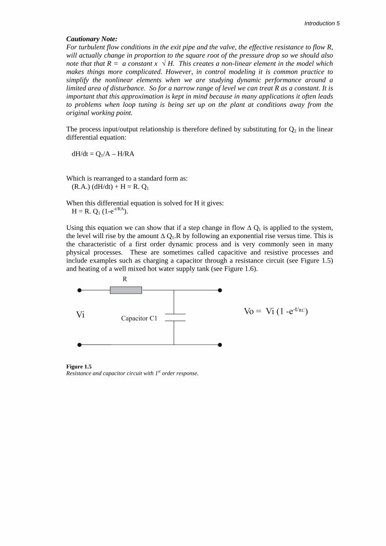
Using this equation we can show that if a step change in flow ∆ Q1 is applied to the system, the level will rise by the amount ∆ Q1.R by following an exponential rise versus time. This is the characteristic of a first order dynamic process and is very commonly seen in many physical processes. These are sometimes called capacitive and resistive processes and include examples such as charging a capacitor through a resistance circuit (see Figure 1.5) and heating of a well mixed hot water supply tank (see Figure 1.6).

Figure 1.5 Resistance and capacitor circuit with 1st order response.


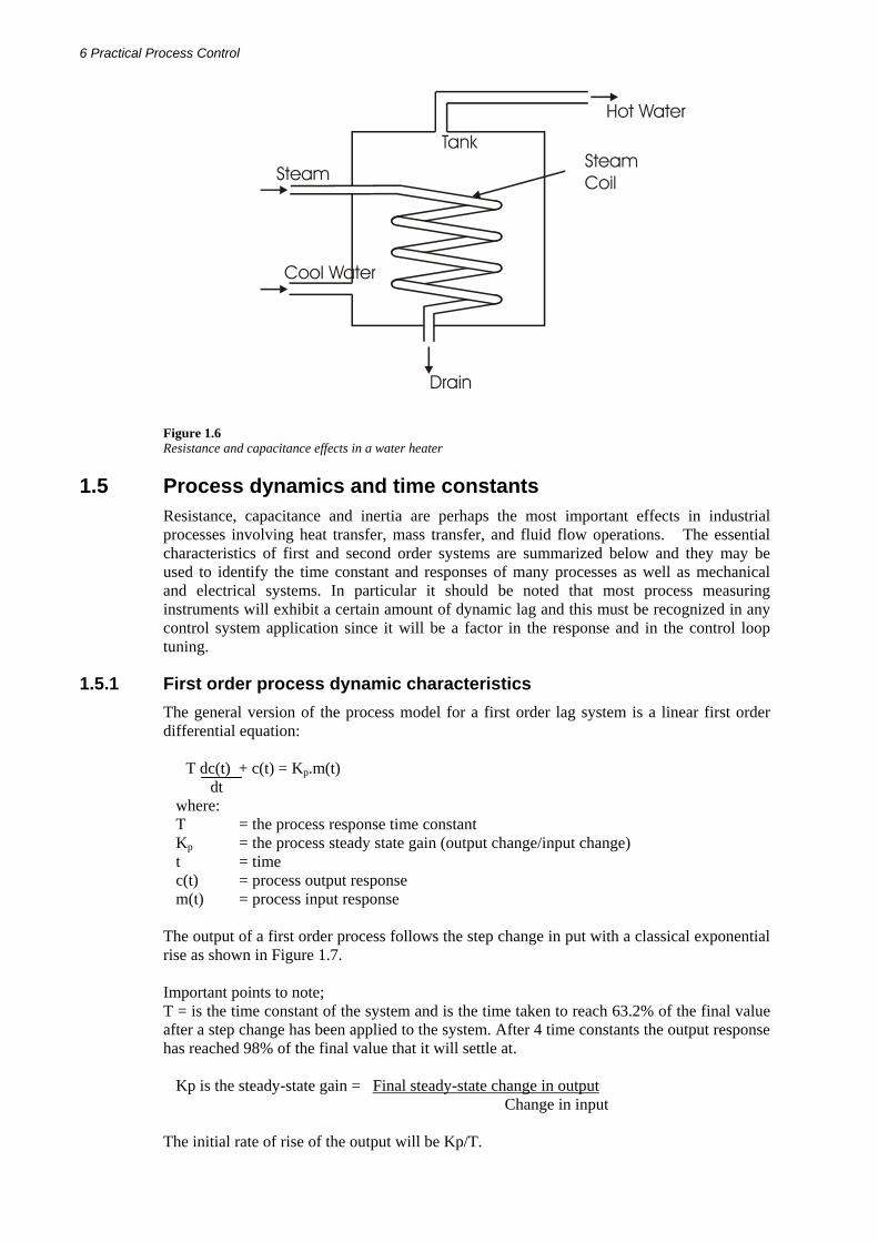
Figure 1.6 Resistance and capacitance effects in a water heater

1.5 Process dynamics and time constants Resistance, capacitance and inertia are perhaps the most important effects in industrial processes involving heat transfer, mass transfer, and fluid flow operations. The essential characteristics of first and second order systems are summarized below and they may be used to identify the time constant and responses of many processes as well as mechanical and electrical systems. In particular it should be noted that most process measuring instruments will exhibit a certain amount of dynamic lag and this must be recognized in any control system application since it will be a factor in the response and in the control loop tuning.

1.5.1 First order process dynamic characteristics The general version of the process model for a first order lag system is a linear first order differential equation:

T dc(t) + c(t) = Kp.m(t) dt where: T = the process response time constant Kp = the process steady state gain (output change/input change) t = time c(t) = process output response m(t) = process input response

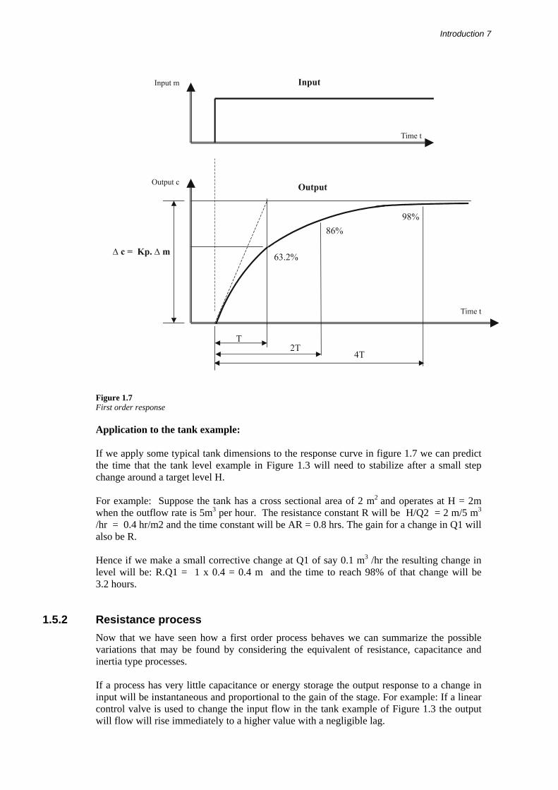
The output of a first order process follows the step change in put with a classical exponential rise as shown in Figure 1.7.

Important points to note;

T = is the time constant of the system and is the time taken to reach 63.2% of the final value after a step change has been applied to the system. After 4 time constants the output response has reached 98% of the final value that it will settle at.

Kp is the steady-state gain = Final steady-state change in output Change in input

The initial rate of rise of the output will be Kp/T.

Introduction 7

Figure 1.7 First order response

Application to the tank example: If we apply some typical tank dimensions to the response curve in figure 1.7 we can predict the time that the tank level example in Figure 1.3 will need to stabilize after a small step change around a target level H. For example: Suppose the tank has a cross sectional area of 2 m2 and operates at H = 2m when the outflow rate is 5m3 per hour. The resistance constant R will be H/Q2 = 2 m/5 m3 /hr = 0.4 hr/m2 and the time constant will be AR = 0.8 hrs. The gain for a change in Q1 will also be R.

Hence if we make a small corrective change at Q1 of say 0.1 m3 /hr the resulting change in level will be: R.Q1 = 1 x 0.4 = 0.4 m and the time to reach 98% of that change will be 3.2 hours.

1.5.2 Resistance process Now that we have seen how a first order process behaves we can summarize the possible variations that may be found by considering the equivalent of resistance, capacitance and inertia type processes. If a process has very little capacitance or energy storage the output response to a change in input will be instantaneous and proportional to the gain of the stage. For example: If a linear control valve is used to change the input flow in the tank example of Figure 1.3 the output will flow will rise immediately to a higher value with a negligible lag.

8 Practical Process Control 1.5.3 Capacitance type processes

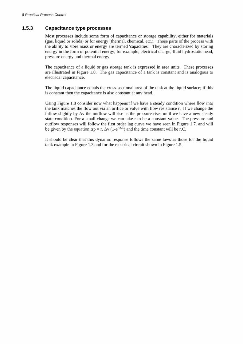
Most processes include some form of capacitance or storage capability, either for materials (gas, liquid or solids) or for energy (thermal, chemical, etc.). Those parts of the process with the ability to store mass or energy are termed 'capacities'. They are characterized by storing energy in the form of potential energy, for example, electrical charge, fluid hydrostatic head, pressure energy and thermal energy. The capacitance of a liquid or gas storage tank is expressed in area units. These processes are illustrated in Figure 1.8. The gas capacitance of a tank is constant and is analogous to electrical capacitance. The liquid capacitance equals the cross-sectional area of the tank at the liquid surface; if this is constant then the capacitance is also constant at any head. Using Figure 1.8 consider now what happens if we have a steady condition where flow into the tank matches the flow out via an orifice or valve with flow resistance r. If we change the inflow slightly by Δv the outflow will rise as the pressure rises until we have a new steady state condition. For a small change we can take r to be a constant value. The pressure and outflow responses will follow the first order lag curve we have seen in Figure 1.7. and will be given by the equation Δp = r. Δv (1-e-t/r.C) and the time constant will be r.C. It should be clear that this dynamic response follows the same laws as those for the liquid tank example in Figure 1.3 and for the electrical circuit shown in Figure 1.5.

Introduction 9

Figure 1.8 Capacitance of a liquid or gas storage tank expressed in area units

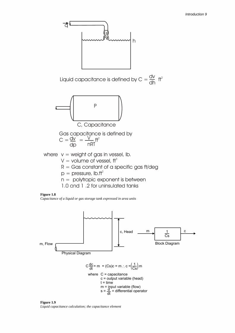
Figure 1.9 Liquid capacitance calculation; the capacitance element


A purely capacitive process element can be illustrated by a tank with only an inflow connection such as Figure 1.9. In such a process, the rate at which the level rises is inversely proportional to the capacitance and the tank will eventually flood. For an initially empty tank with constant inflow, the level c is the product of the inflow rate m and the time period of charging t divided by the capacitance of the tank C.

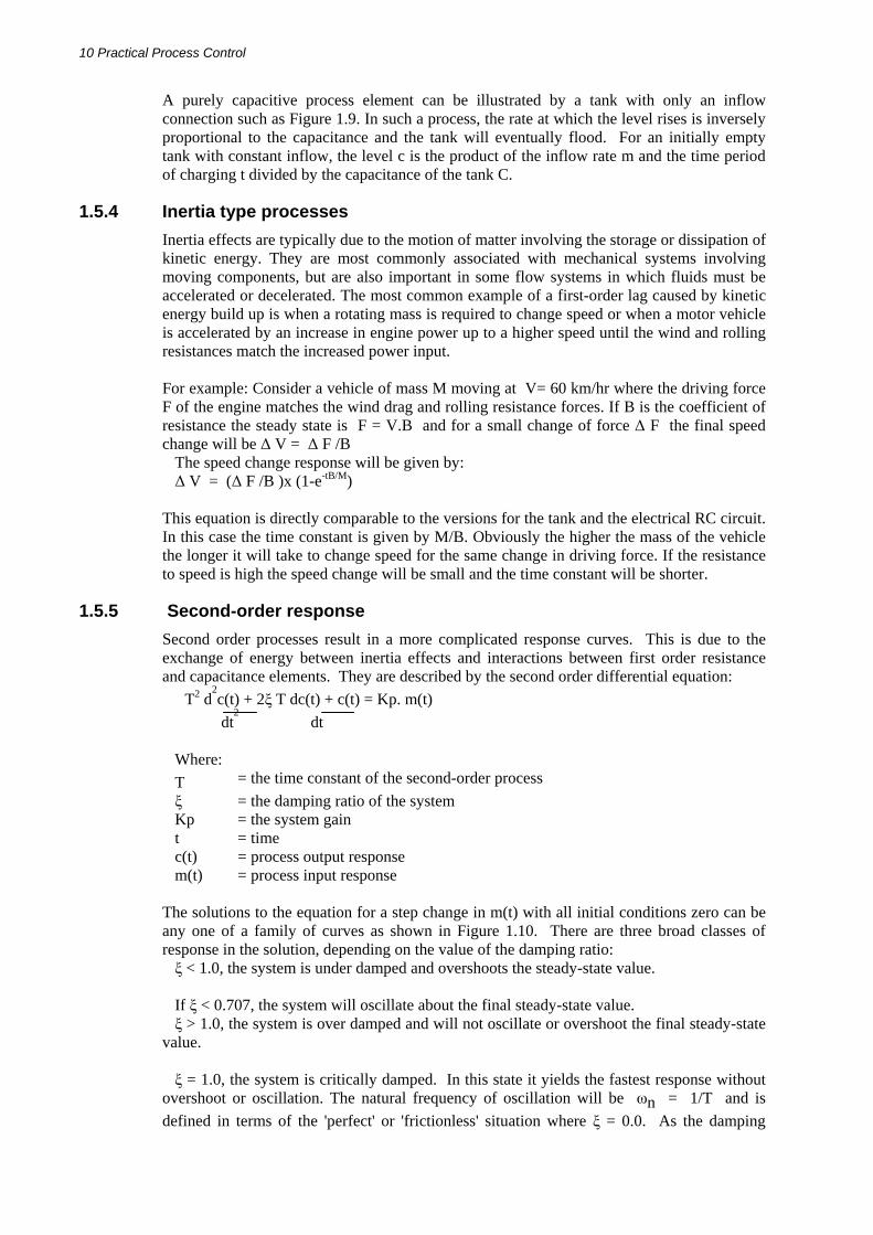
1.5.4 Inertia type processes Inertia effects are typically due to the motion of matter involving the storage or dissipation of kinetic energy. They are most commonly associated with mechanical systems involving moving components, but are also important in some flow systems in which fluids must be accelerated or decelerated. The most common example of a first-order lag caused by kinetic energy build up is when a rotating mass is required to change speed or when a motor vehicle is accelerated by an increase in engine power up to a higher speed until the wind and rolling resistances match the increased power input. For example: Consider a vehicle of mass M moving at V= 60 km/hr where the driving force F of the engine matches the wind drag and rolling resistance forces. If B is the coefficient of resistance the steady state is F = V.B and for a small change of force Δ F the final speed change will be Δ V = Δ F /B

The speed change response will be given by: Δ V = (Δ F /B )x (1-e-tB/M)

This equation is directly comparable to the versions for the tank and the electrical RC circuit. In this case the time constant is given by M/B. Obviously the higher the mass of the vehicle the longer it will take to change speed for the same change in driving force. If the resistance to speed is high the speed change will be small and the time constant will be shorter.

1.5.5 Second-order response Second order processes result in a more complicated response curves. This is due to the exchange of energy between inertia effects and interactions between first order resistance and capacitance elements. They are described by the second order differential equation:

T2 d2c(t) + 2ξ T dc(t) + c(t) = Kp. m(t)

dt2 dt

Where: T = the time constant of the second-order process ξ = the damping ratio of the system Kp = the system gain t = time c(t) = process output response m(t) = process input response

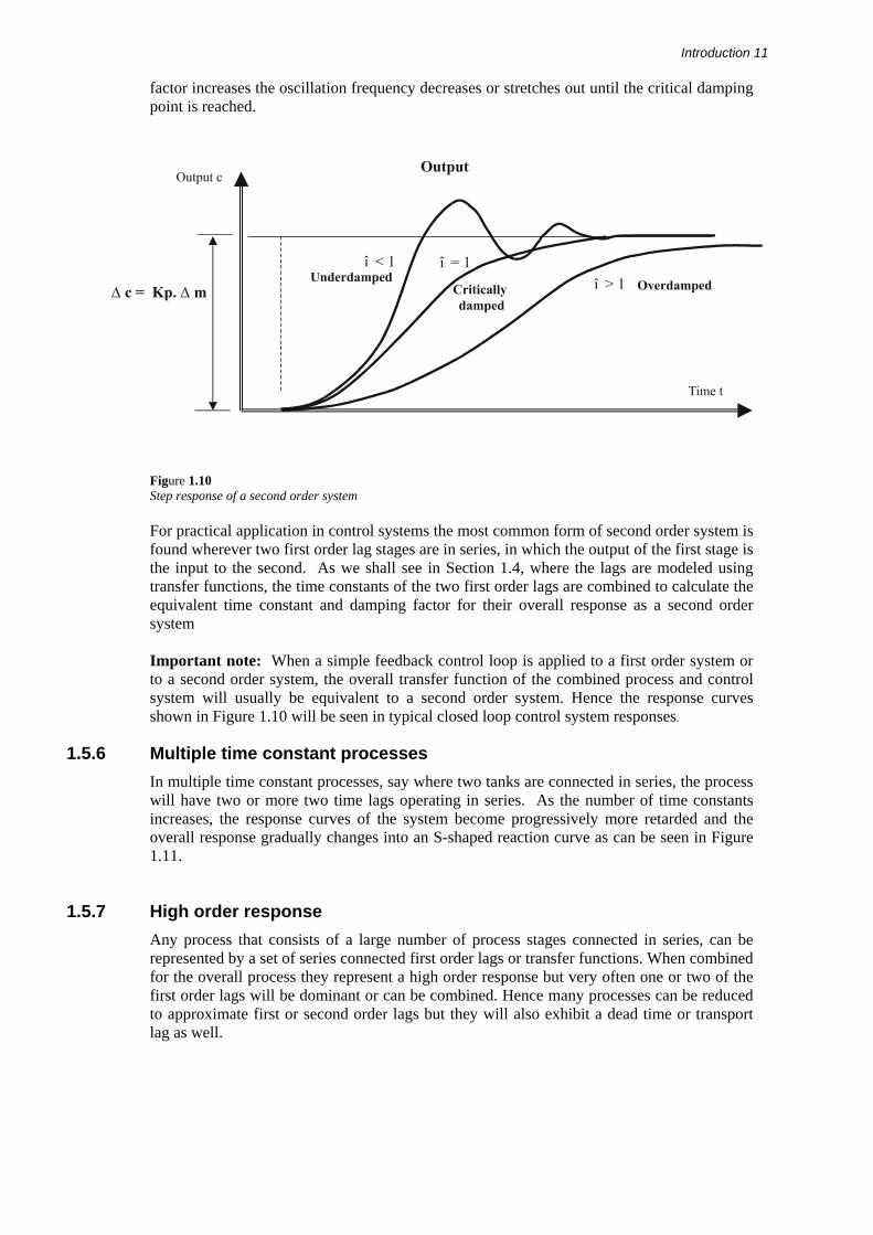
The solutions to the equation for a step change in m(t) with all initial conditions zero can be any one of a family of curves as shown in Figure 1.10. There are three broad classes of response in the solution, depending on the value of the damping ratio: ξ < 1.0, the system is under damped and overshoots the steady-state value. If ξ < 0.707, the system will oscillate about the final steady-state value. ξ > 1.0, the system is over damped and will not oscillate or overshoot the final steady-state

value. ξ = 1.0, the system is critically damped. In this state it yields the fastest response without

overshoot or oscillation. The natural frequency of oscillation will be ωn = 1/T and is defined in terms of the 'perfect' or 'frictionless' situation where ξ = 0.0. As the damping

Introduction 11

factor increases the oscillation frequency decreases or stretches out until the critical damping point is reached.

Figure 1.10 Step response of a second order system

For practical application in control systems the most common form of second order system is found wherever two first order lag stages are in series, in which the output of the first stage is the input to the second. As we shall see in Section 1.4, where the lags are modeled using transfer functions, the time constants of the two first order lags are combined to calculate the equivalent time constant and damping factor for their overall response as a second order system Important note: When a simple feedback control loop is applied to a first order system or to a second order system, the overall transfer function of the combined process and control system will usually be equivalent to a second order system. Hence the response curves shown in Figure 1.10 will be seen in typical closed loop control system responses.

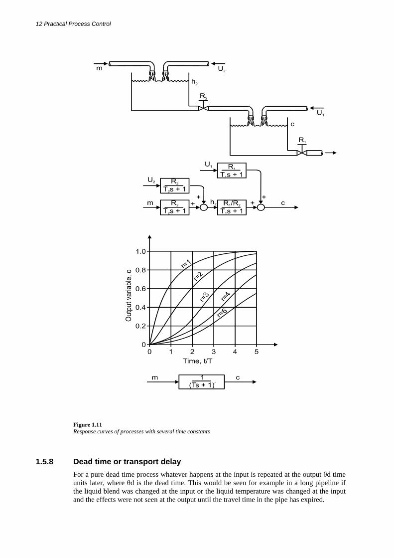
1.5.6 Multiple time constant processes In multiple time constant processes, say where two tanks are connected in series, the process will have two or more two time lags operating in series. As the number of time constants increases, the response curves of the system become progressively more retarded and the overall response gradually changes into an S-shaped reaction curve as can be seen in Figure 1.11.

1.5.7 High order response Any process that consists of a large number of process stages connected in series, can be represented by a set of series connected first order lags or transfer functions. When combined for the overall process they represent a high order response but very often one or two of the first order lags will be dominant or can be combined. Hence many processes can be reduced to approximate first or second order lags but they will also exhibit a dead time or transport lag as well.


Figure 1.11 Response curves of processes with several time constants

1.5.8 Dead time or transport delay For a pure dead time process whatever happens at the input is repeated at the output θd time units later, where θd is the dead time. This would be seen for example in a long pipeline if the liquid blend was changed at the input or the liquid temperature was changed at the input and the effects were not seen at the output until the travel time in the pipe has expired.

Introduction 13

In practice, the mathematical analysis of uncontrolled processes containing time delays is relatively simple but a time delay, or a set of time delays, within a feedback loop tends to lend itself to very complex mathematics. In general, the presence of time delays in control systems reduces the effectiveness of the controller. In well-designed systems the time delays (deadtimes) should be kept to the minimum.

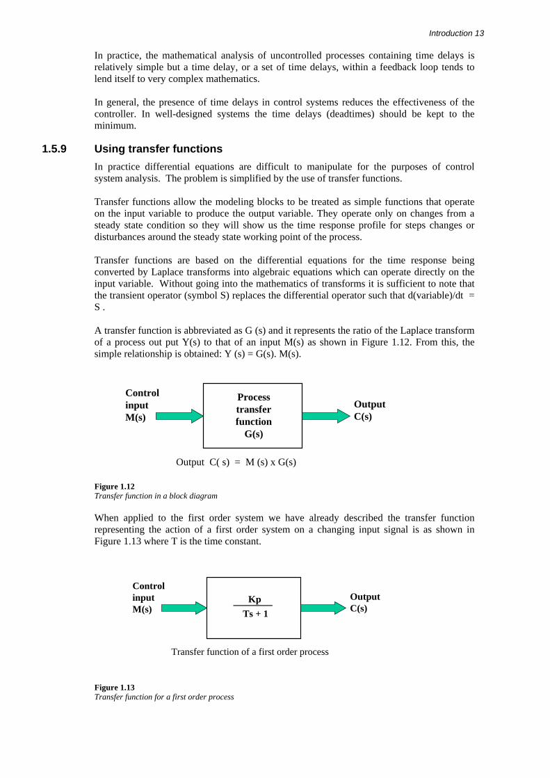
1.5.9 Using transfer functions In practice differential equations are difficult to manipulate for the purposes of control system analysis. The problem is simplified by the use of transfer functions. Transfer functions allow the modeling blocks to be treated as simple functions that operate on the input variable to produce the output variable. They operate only on changes from a steady state condition so they will show us the time response profile for steps changes or disturbances around the steady state working point of the process. Transfer functions are based on the differential equations for the time response being converted by Laplace transforms into algebraic equations which can operate directly on the input variable. Without going into the mathematics of transforms it is sufficient to note that the transient operator (symbol S) replaces the differential operator such that d(variable)/dt = S . A transfer function is abbreviated as G (s) and it represents the ratio of the Laplace transform of a process out put Y(s) to that of an input M(s) as shown in Figure 1.12. From this, the simple relationship is obtained: Y (s) = G(s). M(s).

Figure 1.12 Transfer function in a block diagram

When applied to the first order system we have already described the transfer function representing the action of a first order system on a changing input signal is as shown in Figure 1.13 where T is the time constant.

Figure 1.13 Transfer function for a first order process

Output C( s) = M (s) x G(s)

Control input M(s)

Process transfer function

G(s)

Output C(s)

Transfer function of a first order process

Control input M(s)

Kp Output C(s)Ts + 1


As we have already seen many processes involve the series combination of two or more first order lags. These are represented in the transfer function blocks as seen in Figure 1.14. If the two blocks are combined by multiplying the functions together they can be seen to form a second order system as shown here and as described in Section 1.4.5.

Figure 1.14 Two lags in series combine to produce a 2nd order system

Block diagram modeling of the control system proceeds in the same manner as for the process and is shown by adding the feedback controller as one or more transfer function blocks. The most useful rule for constructing the transfer function of a feedback control loop is shown in Figure 1.15.

Figure 1.15 Block diagram and transfer function for a typical feedback control system

The feedback transfer function H(s) (typically the sensor response) and the controller transfer function Gc(S) are combined in the model to give an overall transfer function that can be used to calculate the overall behavior of the controlled process.

Two first order lags in seriesTwo first order lags in seriesControl input M(s)

K1Output C(s)T1s + 1

K2

T2s + 1

T1T2s2 + 2ξ(T1+T1)s + 1

K1 K2

M(s) Process transfer

function Gp(s)

Output C(s)

Feedback transfer

function H(s)

Combined transfer function: C(s) Gc(s).Gp(s) R(s) 1+G(s).Gp(s).H(s)

=Combined transfer function: C(s) Gc(s).Gp(s)

R(s) 1+G(s).Gp(s).H(s) =

Controller transfer

function Gc(s)

+_

R(s)

Introduction 15

This allows the complete control system working with its process to be represented in a equation known as the closed loop transfer function. The denominator of the right hand side of this equation is known as the open loop transfer function. You can see that if this denominator becomes equal to zero the output of the process approaches infinity and the whole process is seen to be unstable. Hence control engineering studies place great emphasis on detecting and avoiding the condition where the open loop transfer function becomes negative and the control system becomes unstable.

1.6 Types or modes of operation of process control systems There are five basic forms of control available in Process Control. These are:

• On-Off • Modulating • Open Loop • Feed Forward • Closed loop

The next five sections; 1.6.1 to 1.6.5; examine each of these in turn.

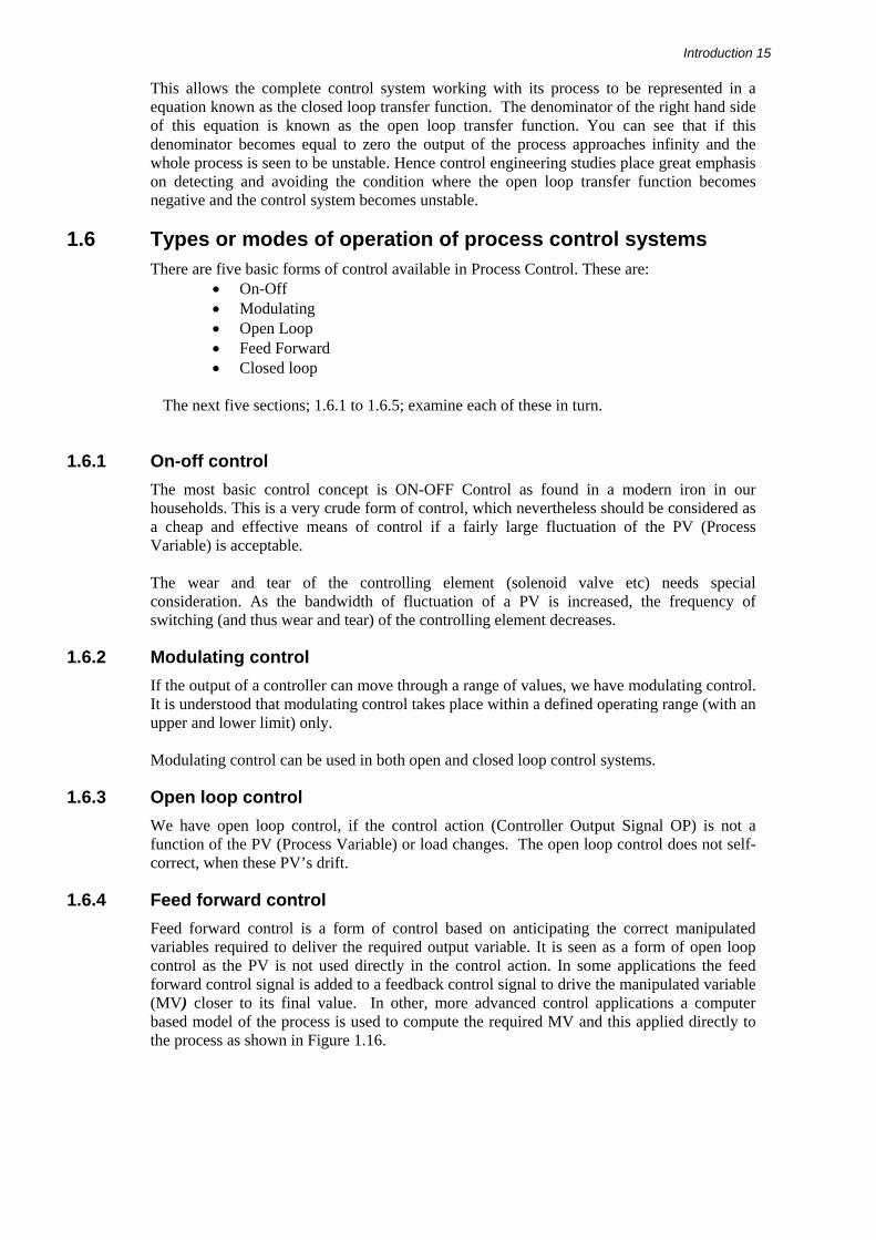
1.6.1 On-off control The most basic control concept is ON-OFF Control as found in a modern iron in our households. This is a very crude form of control, which nevertheless should be considered as a cheap and effective means of control if a fairly large fluctuation of the PV (Process Variable) is acceptable. The wear and tear of the controlling element (solenoid valve etc) needs special consideration. As the bandwidth of fluctuation of a PV is increased, the frequency of switching (and thus wear and tear) of the controlling element decreases.

1.6.2 Modulating control If the output of a controller can move through a range of values, we have modulating control. It is understood that modulating control takes place within a defined operating range (with an upper and lower limit) only.

Modulating control can be used in both open and closed loop control systems.

1.6.3 Open loop control We have open loop control, if the control action (Controller Output Signal OP) is not a function of the PV (Process Variable) or load changes. The open loop control does not self-correct, when these PV’s drift.

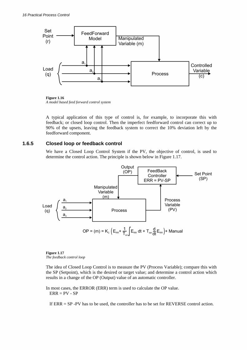
1.6.4 Feed forward control Feed forward control is a form of control based on anticipating the correct manipulated variables required to deliver the required output variable. It is seen as a form of open loop control as the PV is not used directly in the control action. In some applications the feed forward control signal is added to a feedback control signal to drive the manipulated variable (MV) closer to its final value. In other, more advanced control applications a computer based model of the process is used to compute the required MV and this applied directly to the process as shown in Figure 1.16.


Figure 1.16 A model based feed forward control system

A typical application of this type of control is, for example, to incorporate this with feedback; or closed loop control. Then the imperfect feedforward control can correct up to 90% of the upsets, leaving the feedback system to correct the 10% deviation left by the feedforward component.

1.6.5 Closed loop or feedback control We have a Closed Loop Control System if the PV, the objective of control, is used to determine the control action. The principle is shown below in Figure 1.17.

Figure 1.17 The feedback control loop

The idea of Closed Loop Control is to measure the PV (Process Variable); compare this with the SP (Setpoint), which is the desired or target value; and determine a control action which results in a change of the OP (Output) value of an automatic controller.

In most cases, the ERROR (ERR) term is used to calculate the OP value.

ERR = PV - SP If ERR = SP -PV has to be used, the controller has to be set for REVERSE control action.

Introduction 17

1.7 Closed loop controller and process gain calculations In designing and setting up practical process control loops one of the most important tasks is to establish the true factors making up the loop gain and then to calculate the gain. Typically the constituent parts of the entire loop will consist of a minimum of 4 functional items;

Process Gain: ( KP )MVPV

ΔΔ

=

Controller Gain :( KC )E

MVΔΔ

=

The measuring transducer or Sensor gain (refer to Chapter 2), KS and

The Valve Gain KV . The total loop gain is the product of these four operational blocks.

For simple loop tuning two basic methods have been in use for many years. The Zeigler and Nichols method is called the “Ultimate cycle method” and requires that the controller should first be set up with proportional only control. The loop gain is adjusted to find the ultimate gain, Ku. This is the gain at which the MV begins to sustain a permanent cycle. For a proportional only controller the gain is then reduced to 0.5 Ku. Therefore for this tuning the loop gain must be considered in terms of the sum of the four gains given above and the tuning condition is given by the following equation :

KLOOP = ( KC × KP ) = (E

PVMVPVX

EMV

ΔΔ

=ΔΔ

ΔΔ

) x KS x KV = 0.5 x Ku

Normally only the controller gain can be changed but it remains very important that the

other gain components be recognized and calculated. In particular the valve gain and process gain may change substantially with the working point of the process and this is the cause of many of the tuning problems encountered on process plants. Other gain settings are used in the Zeigler and Nichols method for PI and PID controllers to ensure stability when integral and derivative actions are added to the controller. See the next section for the meaning of these terms. The alternative tuning method is known as the 1/4 damping method. This suggests that the controller gain should be adjusted to obtain an under-damped overshoot response having a quarter amplitude of the initial step change in set point. Subsequent oscillations then decay with 1/4 of the amplitude of the previous overshoot. This method does not change the gain settings as integral and derivative terms (see next section) are added in to the controller.

Cautionary Note:

Rule of thumb guidelines for loop tuning should be treated with reservation since each application has its own special characteristics. There is no substitute for obtaining a reasonably complete knowledge of the type of disturbances that are likely to affect the controlled process and it is essential to agree with the process engineers on the nature of the controlled response that will best suit the process. In some cases the above tuning methods will lead to loop tuning that is too sensitive for the conditions, resulting in high degree of instability.

1.8 Proportional, integral and derivative control modes Most Closed loop Controllers are capable of controlling with three control modes which can be used separately or together:


• Proportional Control (P) • Integral, or Reset Control (I) • Derivative, or Rate Control (D)

The purpose of each of these control modes is as follows:

• Proportional control This is the main and principal method of control. It calculates a control action proportional to the ERROR (ERR) . Proportional control cannot eliminate the ERROR completely.

• Integral Control ...(Reset)

This is the means to eliminate the remaining ERROR or OFFSET value, left from the Proportional action, completely. This may result in reduced stability in the control action.

• Derivative Control ...(Rate)

This is sometimes added to introduce dynamic stability to the control LOOP.

Note: The terms RESET for integral and RATE for derivative control actions are seldom used nowadays.

• Derivative control has no functionality on its own.

The only combinations of the P, I and D modes are: P For use as a basic controller PI Where the offset caused by the P mode is removed PID To remove instability problems that can occur in PI mode PD Used in cascade control; a special application I Used in the primary controller of cascaded systems

1.9 An introduction to cascade control Controllers are said to be "In Cascade" when the output of the first or Primary controller is used to manipulate the set point of another or Secondary controller. When two or more controllers are cascaded, each will have its own measurement input or PV but only the primary controller can have an independent set point (SP) and only the secondary, or the most down-stream controller has an output to the process. Cascade control is of great value where high performance is needed in the face of random disturbances, or where the secondary part of a process contains a significant time lag or has non-linearity.

The principal advantages of cascade control are:

Disturbances occurring in the secondary loop are corrected by the secondary controller before they can effect the primary, or main, variable. The secondary controller can significantly reduce phase lag in the secondary loop thereby improving the speed or response of the primary loop. Gain variations due to non-linearity in the process or actuator in the secondary loop are corrected within that loop. The secondary loop enables exact manipulation of the flow of mass or energy by the primary controller.

Introduction 19

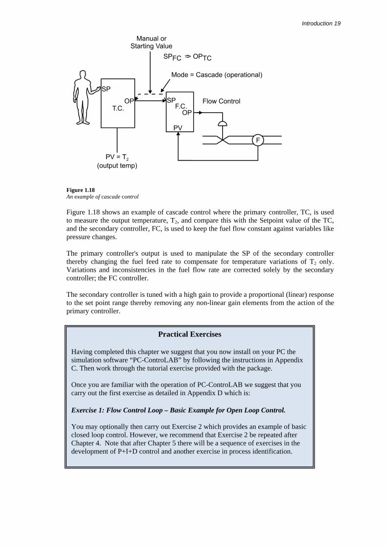
Figure 1.18 An example of cascade control

Figure 1.18 shows an example of cascade control where the primary controller, TC, is used to measure the output temperature, T2, and compare this with the Setpoint value of the TC, and the secondary controller, FC, is used to keep the fuel flow constant against variables like pressure changes. The primary controller's output is used to manipulate the SP of the secondary controller thereby changing the fuel feed rate to compensate for temperature variations of T2 only. Variations and inconsistencies in the fuel flow rate are corrected solely by the secondary controller; the FC controller. The secondary controller is tuned with a high gain to provide a proportional (linear) response to the set point range thereby removing any non-linear gain elements from the action of the primary controller.

Practical Exercises Having completed this chapter we suggest that you now install on your PC the simulation software “PC-ControLAB” by following the instructions in Appendix C. Then work through the tutorial exercise provided with the package. Once you are familiar with the operation of PC-ControLAB we suggest that you carry out the first exercise as detailed in Appendix D which is: Exercise 1: Flow Control Loop – Basic Example for Open Loop Control. You may optionally then carry out Exercise 2 which provides an example of basic closed loop control. However, we recommend that Exercise 2 be repeated after Chapter 4. Note that after Chapter 5 there will be a sequence of exercises in the development of P+I+D control and another exercise in process identification.


Documents

Practical Process Control For Engineers and Technicians · Presents Practical Process Control For Engineers and Technicians Revision 9 Website: E-mail: [email protected]