PRACTICAL IMPLEMENTATION OF A COGNITIVE RADIO SYSTEM FOR

DYNAMIC SPECTRUM ACCESS

A Thesis

Submitted to the Graduate School

of the University of Notre Dame

in Partial Fulfillment of the Requirements

for the Degree of

Master of Science in Electrical Engineering

by

Alice Crohas

J. Nicholas Laneman, Director

Graduate Program in Electrical Engineering

Notre Dame, Indiana

July 2008

PRACTICAL IMPLEMENTATION OF A COGNITIVE RADIO SYSTEM FOR

DYNAMIC SPECTRUM ACCESS

Abstract

by

Alice Crohas

Cognitive radio for dynamic spectrum access enables opportunistic use of the

radio-frequency (RF) spectrum, allowing unlicensed users to utilize licensed bands

under the condition that they interfere as little as possible with the licensees. A

cognitive radio transmits on bands detected as being free, leaving them whenever

a primary user is sensed. This work focuses on the practical implementation of a

cognitive radio for dynamic spectrum access.

A power detector is chosen to sense the spectrum. The Receiver Operating

Characteristic (ROC) of the detector is obtained experimentally. After sensing, the

cognitive radio will transmit on one of the free channels. Detection and transmission

are implemented in parallel at the cognitive transmitter. There is a tradeoff between

transmission rate of the cognitive radio and interference created to the licensed user.

This thesis also presents the implementation of a cognitive receiver, the coun-

terpart to the cognitive transmitter. The cognitive receiver must change frequency

of reception every time the cognitive transmitter changes band (in order to keep

receiving packets). The transmitter sends warning packets when switching from one

channel to another so that the receiver can get resynchronized. Performance of this

cognitive radio system is evaluated using the minimum amount of time necessary

Alice Crohas

for synchronization.

A demonstration system has been set up. Music samples are sent by the cognitive

transmitter and a Graphical User Interface (GUI) shows the state of the channels

(open or in use). Frequency switching is shown to be essentially seamless to the end

user.

CONTENTS

FIGURES . . . . . . . . . . . . . . . . . . . . . . . . . . . . . . . . . . . . . . iv

SYMBOLS . . . . . . . . . . . . . . . . . . . . . . . . . . . . . . . . . . . . . v

CHAPTER 1: INTRODUCTION . . . . . . . . . . . . . . . . . . . . . . . . . 1

CHAPTER 2: BACKGROUND . . . . . . . . . . . . . . . . . . . . . . . . . . 42.1 Definition of Cognitive Radio for Dynamic Spectrum Access . . . . . 42.2 GNU Radio and the USRP . . . . . . . . . . . . . . . . . . . . . . . . 72.3 Spectrum Sensing Techniques . . . . . . . . . . . . . . . . . . . . . . 10

2.3.1 Hypothesis Testing . . . . . . . . . . . . . . . . . . . . . . . . 102.3.2 Models for the Primary User . . . . . . . . . . . . . . . . . . . 102.3.3 Detectors . . . . . . . . . . . . . . . . . . . . . . . . . . . . . 112.3.4 Choice of the Detector . . . . . . . . . . . . . . . . . . . . . . 132.3.5 Spectrum Sensing Techniques Implemented on Testbeds . . . . 14

2.4 OFDM-based Cognitive Radio . . . . . . . . . . . . . . . . . . . . . . 152.5 Synchronization between Cognitive Transmitter and Receiver . . . . . 15

2.5.1 Cyclostationary Signatures for OFDM-based Cognitive Ra-dios and Analog Attention Signal . . . . . . . . . . . . . . . . 16

2.5.2 Choice of the Synchronization Technique in this Work . . . . . 17

CHAPTER 3: IMPLEMENTATION OF A COGNITIVE TRANSMITTERIN GNU RADIO . . . . . . . . . . . . . . . . . . . . . . . . . . . . . . . . 183.1 Setup . . . . . . . . . . . . . . . . . . . . . . . . . . . . . . . . . . . . 183.2 Modulation of the Cognitive Transmitter . . . . . . . . . . . . . . . . 203.3 Parallel Power Detection and Transmission . . . . . . . . . . . . . . . 213.4 Tradeoff in the Cognitive Transmitter . . . . . . . . . . . . . . . . . . 233.5 Implementation of the Transmitter . . . . . . . . . . . . . . . . . . . 253.6 Power Detector . . . . . . . . . . . . . . . . . . . . . . . . . . . . . . 29

3.6.1 Implementation . . . . . . . . . . . . . . . . . . . . . . . . . . 293.6.2 Performance . . . . . . . . . . . . . . . . . . . . . . . . . . . . 32

3.7 List of the Programs used in the Cognitive Transmitter . . . . . . . . 34

ii

CHAPTER 4: COGNITIVE RECEIVER . . . . . . . . . . . . . . . . . . . . . 354.1 Synchronization between Cognitive Transmitter and Receiver . . . . . 364.2 Reception of Packets . . . . . . . . . . . . . . . . . . . . . . . . . . . 374.3 Playing of Music . . . . . . . . . . . . . . . . . . . . . . . . . . . . . 394.4 Performance of the System . . . . . . . . . . . . . . . . . . . . . . . . 394.5 List of the Programs used in the Cognitive Receiver . . . . . . . . . . 414.6 Cognitive Radio Network . . . . . . . . . . . . . . . . . . . . . . . . . 42

CHAPTER 5: CONCLUSION AND FUTURE WORK . . . . . . . . . . . . . 44

BIBLIOGRAPHY . . . . . . . . . . . . . . . . . . . . . . . . . . . . . . . . . 46

iii

FIGURES

2.1 Cognitive Radio Cycle . . . . . . . . . . . . . . . . . . . . . . . . . . 5

2.2 Block Diagram of the USRP . . . . . . . . . . . . . . . . . . . . . . . 8

3.1 Test Setup for Cognitive Radio Implementation and Experiments . . 19

3.2 Graphical User Interface for the Cognitive Transmitter . . . . . . . . 20

3.3 Spectrum Plot of the DBPSK transmission centered at 434 MHz,α=0.35, R=500 kbits/s. The spectrum analyzer plots 20 log(|FFT|)with size of the FFT being 1,024. . . . . . . . . . . . . . . . . . . . . 21

3.4 Parallel Detection and Transmission . . . . . . . . . . . . . . . . . . . 22

3.5 Flow Chart for the Cognitive Transmitter . . . . . . . . . . . . . . . 23

3.6 Format of a Packet . . . . . . . . . . . . . . . . . . . . . . . . . . . . 26

3.7 Flow Graph of the Transmitter Part of the Cognitive Transmitter . . 27

3.8 QPSK Constellation with Gray-Mapping . . . . . . . . . . . . . . . . 29

3.9 Flow Graph of the Power Detector in GNU Radio . . . . . . . . . . . 30

3.10 Receiver Operating Characteristic for the Power Detector . . . . . . . 32

4.1 Flow Chart for the Cognitive Receiver . . . . . . . . . . . . . . . . . 35

4.2 Variables key and pktno . . . . . . . . . . . . . . . . . . . . . . . . . 36

4.3 Flow Graph of the Cognitive Receiver . . . . . . . . . . . . . . . . . . 38

4.4 Path to the Audio Sink . . . . . . . . . . . . . . . . . . . . . . . . . . 39

4.5 Spectrum Plot of two Cognitive Radios and one Primary User . . . . 43

4.6 Spectrum Plot of two Primary Users and one Cognitive Radio . . . . 43

iv

SYMBOLS

N number of samples used for primary user detection

Q size of the FFT

Pd probability of detection

Pf probability of false alarm

M number of PSD frames averaged

S time during which PSD frames are averaged, sensing time

D time during which samples are thrown away, discard time

T transmission time

D′ hardware latency time

fs rate of the samples coming from the FPGA

fmax maximum sampling rate of the USRP

F decimation factor of the FPGA

α roll-off factor

R nominal bit rate of the cognitive radio

Rmusic rate of the music

Tdwell amount of time during which the receiver dwells on a channel

k number of bits per symbol

v

CHAPTER 1

INTRODUCTION

A large portion of the assigned radio-frequency (RF) spectrum is used sporad-

ically today, resulting in spectral inefficiency. Spectrum utilization is a function of

time and location; it ranges from 15 % to 85 % according to the FCC [2]. A fixed

spectrum allocation prevents rarely used frequencies from being used by unlicensed

users. A proposed solution to this problem is cognitive radio for dynamic spectrum

access.

Cognitive radio used for dynamic spectrum access allows unlicensed users to

utilize licensed bands. Cognitive radios must cause as little interference as possible

to the licensed (or primary) communication; they only transmit on bands they

just sensed as being free. The cognitive receiver must stay synchronized with the

cognitive transmitter when the latter changes channel.

The motivation of this thesis is to practically implement a complete cognitive

radio system. The detector part of the cognitive radio and synchronization between

transmitter and receiver have been implemented and documented on various plat-

forms but to the best of our knowledge, no work describes the implementation of

both cognitive transmitter and receiver on low-cost hardware such as the USRP. The

technique used for synchronization between transmitter and receiver in this work

is simple and does not require the complex calculation of the SCF at the receiver.

Performance of the energy detector is obtained by sending signals over the air from

1

one USRP to another, taking into account all possible sources of interference. A

working demonstration illustrates the potential benefits of dynamic spectrum access

by a cognitive radio on underutilized licensed spectrum. An outline of the thesis is

as follows.

Chapter 2 details the main functions of a cognitive radio and presents the testbed:

GNU Radio, the software architecture, and the Ettus Universal Software Radio

Peripheral (USRP), the hardware. The concept of a flow graph is explained, and

the technical characteristics of the USRP relevant to cognitive radio are presented.

A survey of the detectors used for spectrum sensing is given, including the ones

already implemented in GNU Radio. The choice of the power detector for the

implementation is explained. This chapter also presents the different techniques for

synchronization between a cognitive transmitter and receiver and the choice of the

technique for this work.

Chapter 3 presents the cognitive transmitter. The parallel implementation of the

detector and transmitter is explained. There is a tradeoff between the transmission

rate of the cognitive radio and the interference created to the primary user. The

signal processing blocks used to build the power detector and transmitter in GNU

Radio are given. Performance of the power detector is obtained experimentally using

the Receiver Operating Characteristic (ROC).

Chapter 4 focuses on the cognitive receiver. It presents the protocols used to syn-

chronize transmitter and receiver. Overhead is created at the cognitive transmitter

and receiver to enable coordination. It is shown that there exists a minimum amount

of time necessary for synchronization. This chapter also presents the concept of a

network of cognitive radios.

A demonstration has been set up to show that the cognitive transmitter leaves

the band whenever a primary user is sensed and that the cognitive receiver stays syn-

2

chronized with the transmitter. Possible improvements on the system are described

in Chapter 5.

3

CHAPTER 2

BACKGROUND

In this chapter, the definition of a cognitive radio for dynamic spectrum access

is given and the hardware and software used in the implementation are described.

There exist different detectors for sensing the spectrum in the literature; their per-

formances are compared. A power detector is chosen for the practical implementa-

tion of the cognitive radio. Two techniques for synchronization between cognitive

transmitter and receiver are detailed: cyclostationary signature for OFDM-based

cognitive system and analog attention signal. Finally, the choice of the synchroniza-

tion technique in this work is explained.

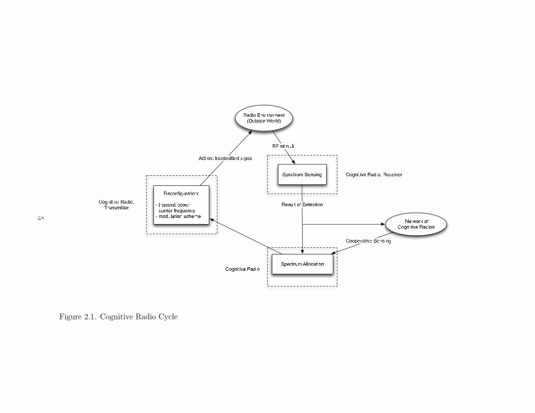
2.1 Definition of Cognitive Radio for Dynamic Spectrum Access

The concept of dynamic spectrum access is to identify spectrum holes or white

spaces and use them to communicate. A cognitive radio is a “smart” radio platform.

White spaces change over time: a cognitive radio used for dynamic spectrum access

“jumps” from one chunk of spectrum to another.

Figure 2.1 represents the different actions taken by a cognitive radio as well as

its interaction with the outside environment. It is based on Figure 1 in [9] and on

[1].

4

Ra d io En v ir o n m en t( Ou ts i d e Wo r l d )S p e c tr u mS en s i n gR F s t i m u l i Co g n i t i v e Ra d io, R e c e i v er

N e tw o r k o fCo g n i t i v e Ra d io s

S p e c tr u m A l lo ca t io n

R e co n fi g u r a t io n :! tr a n s m i t po w er! ca r r i er fr e q u en c y! mo d u l a t io n s c h e m eCo g n i t i v e Ra d io,Tr a n s m i t t er R e s u l t o f D e t e c t io nCo o p er a t i v eS en s i n g

A c t io n : tr a n s m i t t e d s i g n a lCo g n i t i v e Ra d io

Figure 2.1. Cognitive Radio Cycle

5

The main functions of a cognitive radio used for accessing the spectrum oppor-

tunistically are:

• spectrum sensing

• spectrum allocation

• reconfiguration

• transmission

The first step, spectrum sensing, determines if a primary user is present on a band.

After sensing the spectrum, the cognitive radio can share the result of its detection

with other cognitive radios. Cooperative spectrum sensing is studied for example in

[7], [4] and references therein. Cooperative sensing can be centralized (a base station

gathers all sensing information, detects spectrum holes and indicates to the cognitive

radios where to transmit) or decentralized (secondary users exchange measurements

and decide which band to use).

Cooperative sensing is a solution to the “hidden node problem”. The hidden node

problem occurs when a primary user is far away from the cognitive transmitter (it

is not detected) but close to the receiver. The receiver will not receive the samples

correctly because the cognitive transmitter and primary user transmit on the same

band. With cooperative spectrum sensing, cognitive users closer to the licensed

system will help the ones far away from it [6].

The second step followed by the cognitive radio is spectrum allocation, when it

decides which band to use. If multiple secondary users are present, they must share

the available spectrum.

Finally, the cognitive radio reconfigures itself to transmit in the open band,

potentially changing its carrier frequency, transmit power and modulation scheme

(to better match the available band). Reconfiguration must occur quickly to ensure

seamless communication during the transition from one band to another.

6

2.2 GNU Radio and the USRP

In this work, the cognitive radio is implemented in software, making it a software-

defined radio (SDR). The amount of hardware used is minimal and processing of

the samples is done in software. Changing the functionalities of the radio is easily

done by changing the code instead of the hardware.

The software architecture is the GNU Radio open source software available at

www.gnu.org/software/gnuradio. GNU Radio uses two programming languages:

Python and C++. Python provides a higher level of abstraction than C++. The

top-level specification of an algorithm is a flow graph written in Python. A flow

graph is a series of interconnected blocks; the blocks are written in C++. A block

can be a source, a sink, or an intermediate signal processing block. Often the USRP

is either the beginning of the flow graph (implementation of a receiver) or the end

(transmitter). Processing of the samples coming from the hardware is done inside

the blocks. The creation of an application in GNU Radio consists in first creating

C++ blocks and then writing a class flow graph in Python that connects the blocks.

Once the flow graph is started, its components cannot be changed and samples flow

from the source to the sink. The SWIG library provides an interface between Python

and C++, and wxPython is used to create Graphical User Interfaces (GUIs).

The hardware used to implement the cognitive radio is the Universal Software

Radio Peripheral (USRP) available from Ettus Research LLC (www.ettus.com).

The USRP is comprised of two receive daughterboards, two transmit daughter-

boards, four Analog to Digital Converter (ADCs), four Digital to Analog Converter

(DACs), and one Field Programmable Gate Array (FPGA). In this work, we use the

400 MHz receive and transmit daughterboards: the range of the signals is 400-500

MHz. Figure 2.2 is a simplified diagram of the blocks in the USRP. In the receive

daughterboard, the goal is to translate the desired signal centered at frequency ωD

7

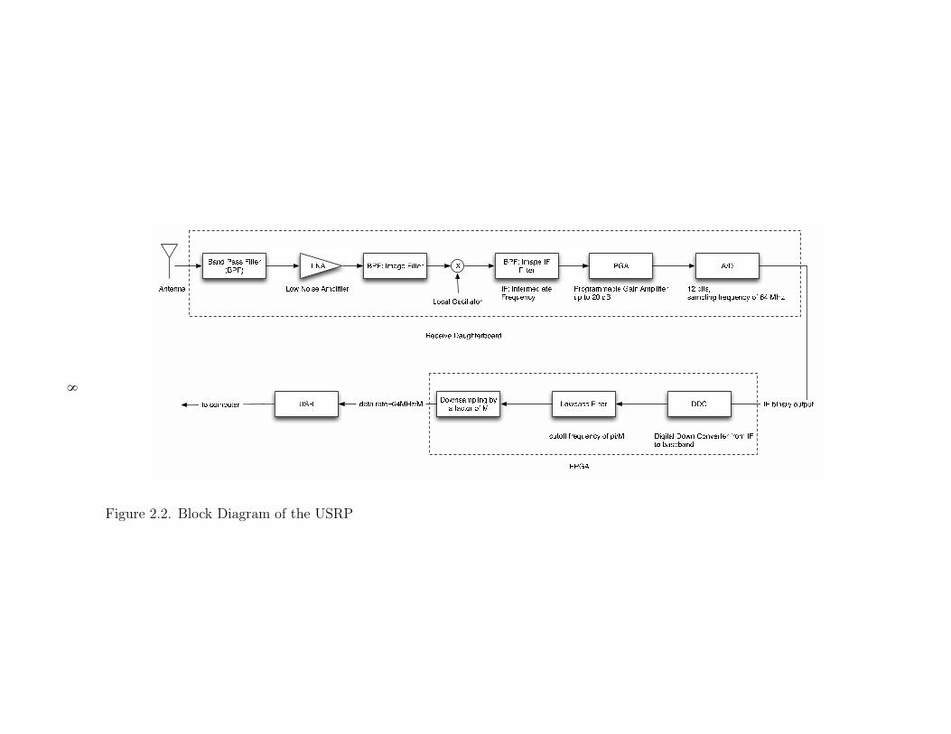
Ba n d P a s s F i lt e r( B P F ) L N A B P F: I m a g e F i lt e r X B P F: I m a g e I FF i lt e r P G A A / DD D CLo w p a s s F i lt e rD o w n sa m p l i n g bya fa ct o r o f MU S B

A nt e n n a Lo w N o i s e A m p l i fi e r Lo ca l O s c i l l a t o r P ro g ra m m a b l e G a i n A m p l i fi e ru p t o 2 0 d B 1 2 b it s,sa m p l i n g f r e q u e n cy o f 6 4 M HzI F b i n a ry o ut p ut

I F: I nt e r m e d i a t eF r e q u e n cyD i g it a l D o w n C o n v e rt e r f ro m I Ft o ba s e ba n dc ut o f f f r e q u e n cy o f p i / Md a t a ra t e= 6 4 M Hz / Mt o co m p ut e r

R e c e i v e D a u g ht e r b o a r dF P G A

Figure 2.2. Block Diagram of the USRP

8

to an Intermediate Frequency (IF, ωIF ) so that the signal can be sampled at a rea-

sonable rate. The maximum sampling frequency fmax offered by the USRP is 64

MHz. After mixing with the local oscillator, the desired spectrum is translated to

IF because the frequency of the local oscillator is:

ωLO = ωD − ωIF

The image filter removes the harmonics at ωIF − ωLO. Indeed, these harmonics

would otherwise get translated to ωIF after mixing with the local oscillator and

interfere with the desired signal. The image IF filter only keeps the harmonics at

ωIF , i.e., the desired signal.

After translation to IF, the signal is passed through the ADC. The role of the

FPGA is to further downconvert the incoming signal centered around the IF to

baseband and to reduce the sampling rate with a downsampler. The data rate of

the samples entering the Universal Serial Bus (USB) is

fs =fmax

F

with F the decimation factor. USB 2.0 can support data rates up to 32 Mbytes/s,

i.e., 8 M complex samples/s, since the size of a complex sample is 4 bytes (16 bits for

In phase (I) component and 16 bits for Quadrature (Q) component). The decimation

factor F must be at least 8 in order to transmit complex samples across the USB 2.0

(648

= 8). The maximum rate of the samples coming from the USB is 8 M samples/s

and therefore, by Nyquist’s theorem, the maximum baseband bandwidth sensed by

the cognitive radio at a time is 4 MHz.

9

2.3 Spectrum Sensing Techniques

This section presents the problem of detecting the primary user. Several de-

tectors are discussed in the literature and their performances are compared. This

section also notes the detectors already implemented in GNU Radio and explains

the choice of the detector for the implementation.

2.3.1 Hypothesis Testing

Detection is based on the complex baseband signal coming from the FPGA. Dur-

ing the spectrum sensing phase, the cognitive radio decides between two hypotheses:

H0 : primary user not present

HS : primary user present

The most common models for the signal under H0 and HS are of the form

H0 : Yn = Wn, n = 1, . . .N

HS : Yn = Xn + Wn, n = 1, . . . N,

where Yn is a two-dimensional vector representing the I and Q components of the

signal, Wn is the zero-mean Additive White Gaussian Noise (AWGN) with variance

σw2, Xn is the signal sent by the primary user(s), independent of the noise, and N

is the number of complex samples used for detection of the primary user.

2.3.2 Models for the Primary User

In the literature, the primary user (Xn) is modeled in different ways:

• Xn is a random vector for every n. The primary user’s symbol constellationis known to the cognitive radio [13]. Detection is then based on the samplesafter the matched filter but before the slicer.

• Xn is modeled as a zero-mean, rotationally symmetric, complex Gaussian pro-cess. This model is motivated by the central limit theorem (the signal receivedis the sum of many primary users’ signals [10]). In this case, the covariancematrix of Xn is known to the cognitive radio.

10

• Xn is a deterministic signal. The detector knows the entire signal [8] or onlythe signal power [5].

For our purpose, model 1 is appropriate since a USRP using Differential Binary

Phase Shift Keying (DBPSK) will serve as the primary user for the plotting of the

ROC of the power detector. However, for convenience, a Push To Talk (PTT) using

Frequency Modulation (FM) will play the role of the primary user in the experiments

with the cognitive radio system.

2.3.3 Detectors

Different detectors can be used to detect primary users, e.g. a Likelihood Ratio

Test (LRT), a power detector, or a cyclostationary feature detector. Let Pd denote

the probability of detection and Pf the probability of false alarm. For dynamic

spectrum access, the probability of missed detection 1−Pd must be minimized, en-

suring that the secondary user causes as little interference as possible to the primary

user. Hence the Neyman-Pearson criterion is used as a performance objective for

cognitive radio applications.

Likelihood Ratio Test

This detector is used when the cognitive radio knows the primary user’s signal

(when it is deterministic) or the symbols and their probabilities (when it is random).

It requires a good model of the primary signal. If the probability density functions

(pdfs) of the signal and the noise are accurately known, then the LRT is the optimal

Neyman-Pearson detector.

11

Power Detector

Yn is now assumed to be a one-dimensional real signal. This detector uses the

following statistic:

S(Y ) =N

∑

i=1

Yi2 (2.1)

The decision rule will then take the following form:

S(Y )HS

≷H0

λ

where λ is a decision threshold. To obtain expressions for Pd and Pf , the licensed

user’s signal is modeled as being deterministic (N∑

i=1

xi2 known) or as being a zero-

mean Gaussian process with known variance σx2.

Expressions for Pd and Pf can be found without knowing the entire primary

user’s signal. When the noise is AWG, the statistic S(Y )σw

2 has a central chi-square

distribution with N degrees of freedom (assuming H0). This statistic has a non-

central chi-square distribution with non-centrality parameter the SNR (

NP

i=1

xi2

σw2 ) and

same degrees of freedom, assuming HS and that the licensed user’s signal is deter-

ministic. Pd and Pf are then functions of λ, SNR and N [5].

If the licensed user’s signal is a zero-mean Gaussian process, then the statistic

S(Y )σw

2+σx2 has a central chi-square distribution (assuming HS). If in addition, N is

assumed to be large, the central limit theorem applies, and we have the following

relationship between Pd, Pf , SNR and N [3]:

N = 2[(Q−1(Pf) − Q−1(Pd))SNR−1 − Q−1(Pd)]2 (2.2)

where the SNR is defined as σx2

σw2 .

12

Cyclostationary Feature Detector

Cyclostationary processes are random processes whose mean and autocorrelation

are periodic functions of time. Most modulated signals are cyclostationary due to

sine wave carriers, symbol pulse shaping, cyclic prefixes and so forth [2]. Cyclosta-

tionary signals exhibit spectral redundancy: there is correlation between separated

spectral components. This is why the Spectral Correlation Function (SCF) is used

to distinguish between noise and the primary user (cyclostationary). The SCF is

obtained by correlating the Fast Fourier Transform (FFT) of the signal and aver-

aging over time [2]. The spectral correlation function is a powerful tool because it

shows the number of signals, their modulation type and the symbol rates. However,

reliable detection requires that the SCF be calculated over a wide range of frequen-

cies, which is computationally complex and it also requires long observation times

[14].

2.3.4 Choice of the Detector

For our implementation of a cognitive radio system, we chose to use a power

detector. These are several reasons why a power detector is chosen to sense the

spectrum in our application.

The LRT requires a good model for the primary user’s signal whereas the power

detector only requires the power of the signal. The power detector senses all kinds

of licensed user’s signals; the LRT is tuned to a particular modulation. Moreover,

the LRT requires symbol timing recovery.

The statistic and decision rule for the power detector are not as complex as the

ones used in the cyclostationary feature detector which requires plotting a function

of two variables, the SCF, and to implement an algorithm to look for the primary

user’s features.

13

2.3.5 Spectrum Sensing Techniques Implemented on Testbeds

In [12], an energy detector is implemented in GNU Radio, using the USRP. A

time-averaged PSD (Power Spectral Density) denoted as P (f) is calculated using a

512-point FFT and a Blackman-Harris window. In a preliminary step, the mean µ

and variance σ2 of the PSD are obtained in the absence of a primary signal. These

values are then used to decide if a frequency is open or in use:

frequency is open if P (f) < µ + 0.2σ

frequency is in use if P (f) > µ + 3σ

This method requires the periodic calculation of µ and σ if the noise is non-

stationary. Moreover, for our purposes, we are not interested in making decisions

on a frequency-by-frequency basis. Our goal is to determine if a channel is open or

in use and we want to transmit using its entire bandwidth. We therefore make a

decision by summing the frequencies in that channel.

In [3], a power detector implemented on the Berkeley Emulation Engine 2 (BEE2)

is presented, the statistic used is the same as in formula (2.1). Neither GNU Radio

nor the USRP is used. The testbed BEE2 is an FPGA based platform. The FPGA

is connected to a laptop and the RF front-end is connected to BEE2 via an optical

cable. The front-end is tuned to the ISM band at 2.4 GHz, and the ADC is the

same as the one in the USRP: 12 bits, 64 MHz. Modulated signals are generated

via a signal generator which is controlled by the BEE2. The SNR at the receiver

for a 4 MHz wide QPSK signal centered at 2.4 GHz is between -13 to -25 dB. Pf

and Pd are calculated over 1000 experiments. Pd versus sensing time is plotted for

a Pf of 0.05 and equation 2.2 is verified.

During these experiments, the signal generator is directly connected to the RF

board antenna via an SMA cable: communication is not done over the air and

14

hence, measurements do not take into account possible path loss or outside sources

of interference. In addition, the radio is put inside an RF shield, ensuring that noise

only comes from the radio circuitry. In our implementation, the ROC is obtained

by sending signals over the air, from one USRP to another.

2.4 OFDM-based Cognitive Radio

The Orthogonal Frequency Division Multiplexing (OFDM) provides for a very

flexible frequency management on a carrier-by-carrier basis. This is why OFDM is

interesting for cognitive radio applications. The bandwidth occupied by the OFDM-

based cognitive radio can be shaped by feeding some carriers with zeros in order to

better match the band detected as being open. However, the matching cannot be

perfect since the Fourier transform of a subchannel is not band-limited, it is a sinc-

shaped spectra that can interfere with the licensed user (adjacent channel leakage

effect).

Although OFDM would be an appealing direction for cognitive radio work, the

current GNU Radio implementation is not usable. As a result, single-carrier DBPSK

is used throughout this work.

2.5 Synchronization between Cognitive Transmitter and Receiver

We will now be interested in the cognitive receiver. A cognitive transmitter

senses the spectrum and transmits samples on an available band to a cognitive

receiver. The radio that receives these samples must also be cognitive because it

must change frequency of reception every time the cognitive transmitter changes

band. The transmitter and receiver must be synchronized at all times in order

for the communication link not to be broken. There exist different techniques for

enabling synchronization between the cognitive transmitter and receiver.

15

2.5.1 Cyclostationary Signatures for OFDM-based Cognitive Radios and AnalogAttention Signal

The first technique used for synchronization is to embed a cyclostationary signa-

ture in the signal of the cognitive transmitter and a cyclostationary feature detector

in the receiver.

A cyclostationary feature detector has been implemented in [14]. The testbed

is comprised of a signal generator, USRP and a software radio architecture called

Implementing Radio In Software (IRIS). In order to detect the band used by the

cognitive transmitter, the SCF is calculated at the cognitive receiver. The cog-

nitive transmitter sends OFDM signals embedded with cyclostationary signatures.

Spectral resolution in the SCF must be of the order of the OFDM subcarrier spac-

ing for the cognitive receiver to be able to detect the peaks. A signal generator

is used to generate OFDM signals with QPSK modulated symbols at 2.3405 GHz,

the bandwidth of the transmission is 1 MHz. The cyclostationary feature detector

uses the USRP front-end at 2.34 GHz with 4 MHz bandwidth. Receiver Operating

Characteristics (ROCs) are plotted for a SNR of 0 dB and different observation

times.

Cyclostationary signatures enable the cognitive receiver to get synchronized with

the transmitter. The signature is created by simultaneously transmitting data sym-

bols on more than one subcarrier. The signature can be made specific to a cognitive

transmitter by choosing the number of carriers on which the symbols will be re-

peated. A peak will appear in the SCF of the transmitted signal at the carrier

frequency, allowing the cognitive receiver to reconfigure itself to receive samples at

that frequency.

The cognitive transmitter can also send an analog attention signal to meet with

the receiver [11]. The attention signal is a simple carrier with a small number of

16

sidetones. The cognitive receiver will compute the Fast Fourier Transform (FFT)

and search for that pattern.

2.5.2 Choice of the Synchronization Technique in this Work

Both methods present the advantage that the cognitive receiver does not have

to know a priori the frequency of transmission. However, overhead is created at

the transmitter in both cases: data rate is decreased because the symbols are re-

dundantly transmitted on several subcarriers for the cyclostationary signature tech-

nique, and the analog attention signal does not carry any useful information. Also,

calculating the SCF for a wide range of frequencies is computationally complex, and

the analog attention signal technique requires a good FFT resolution to accurately

detect the frequency of transmission.

In this work, we chose to use a simple technique for synchronization between

cognitive transmitter and receiver that does not require the accurate detection of

the frequency of transmission. The receiver knows the set of frequencies used by the

transmitter and it will dwell on each channel to find the cognitive transmitter.

17

CHAPTER 3

IMPLEMENTATION OF A COGNITIVE TRANSMITTER IN GNU RADIO

This chapter presents the setup of the demonstration of the cognitive system

and explains the parallel implementation of the detection and transmission. There

is a tradeoff at the cognitive transmitter between transmission rate and interference

created to the primary user. The flow graphs of the transmitter and power detector

are detailed and performance of the detector is evaluated with the ROC. Finally,

the list of the programs used for the implementation of the cognitive transmitter is

given.

3.1 Setup

To illustrate how the cognitive radio system works, a test setup has been con-

figured (Figure 3.1). Two software radio prototypes (secondary transmitter and

receiver) and a PTT handheld device (primary user) are used. The prototype is

a portable device consisting of a USRP and an integrated processor running GNU

Radio. The cognitive transmitter senses the spectrum and transmits packetized

music on a channel detected as being free. The cognitive receiver plays the music

samples sent by the transmitter. When the handheld device transmits on the same

channel as the cognitive transmitter, the latter will change channel and the receiver

will get resynchronized on the new channel chosen by the transmitter. Figure 3.2

shows the Graphical User Interface (GUI) for the cognitive transmitter.

18

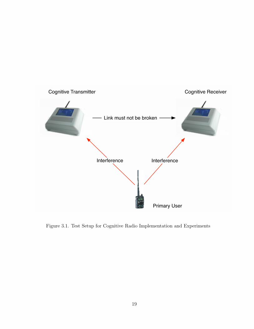
Figure 3.1. Test Setup for Cognitive Radio Implementation and Experiments

19

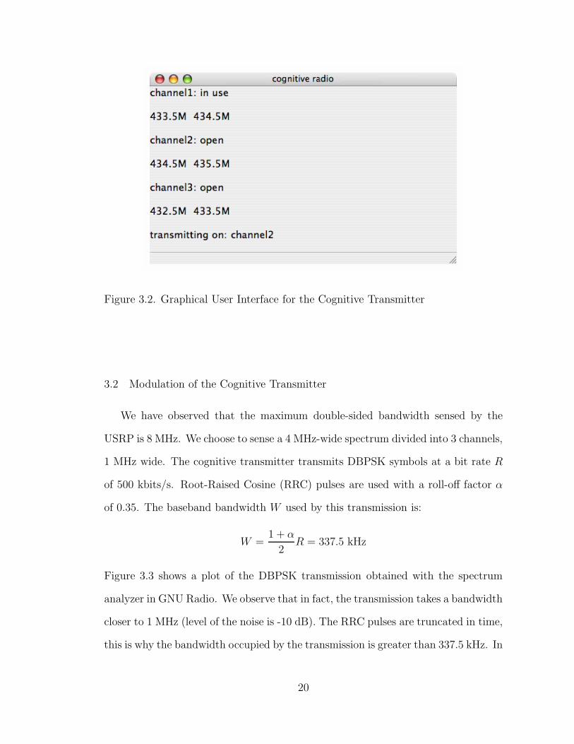
Figure 3.2. Graphical User Interface for the Cognitive Transmitter

3.2 Modulation of the Cognitive Transmitter

We have observed that the maximum double-sided bandwidth sensed by the

USRP is 8 MHz. We choose to sense a 4 MHz-wide spectrum divided into 3 channels,

1 MHz wide. The cognitive transmitter transmits DBPSK symbols at a bit rate R

of 500 kbits/s. Root-Raised Cosine (RRC) pulses are used with a roll-off factor α

of 0.35. The baseband bandwidth W used by this transmission is:

W =1 + α

2R = 337.5 kHz

Figure 3.3 shows a plot of the DBPSK transmission obtained with the spectrum

analyzer in GNU Radio. We observe that in fact, the transmission takes a bandwidth

closer to 1 MHz (level of the noise is -10 dB). The RRC pulses are truncated in time,

this is why the bandwidth occupied by the transmission is greater than 337.5 kHz. In

20

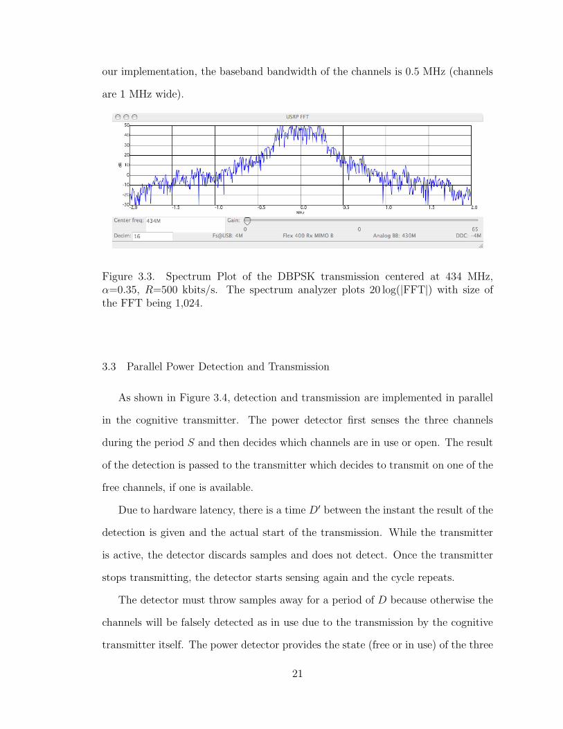
our implementation, the baseband bandwidth of the channels is 0.5 MHz (channels

are 1 MHz wide).

Figure 3.3. Spectrum Plot of the DBPSK transmission centered at 434 MHz,α=0.35, R=500 kbits/s. The spectrum analyzer plots 20 log(|FFT|) with size ofthe FFT being 1,024.

3.3 Parallel Power Detection and Transmission

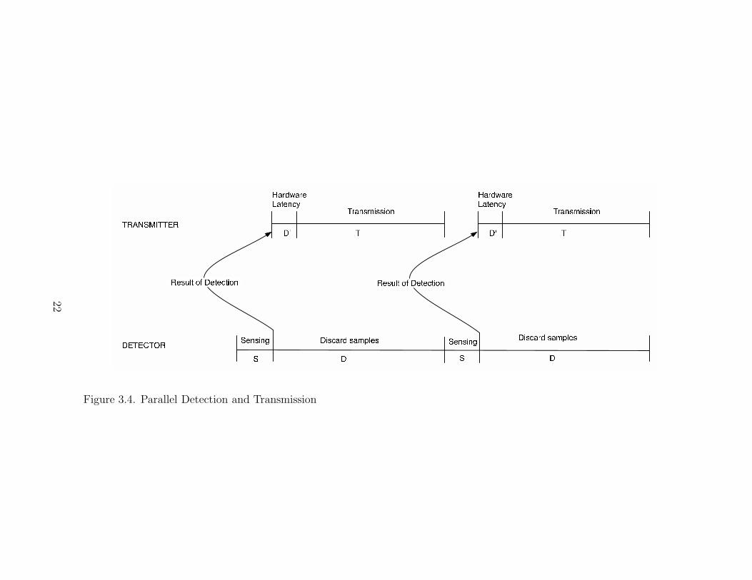
As shown in Figure 3.4, detection and transmission are implemented in parallel

in the cognitive transmitter. The power detector first senses the three channels

during the period S and then decides which channels are in use or open. The result

of the detection is passed to the transmitter which decides to transmit on one of the

free channels, if one is available.

Due to hardware latency, there is a time D′ between the instant the result of the

detection is given and the actual start of the transmission. While the transmitter

is active, the detector discards samples and does not detect. Once the transmitter

stops transmitting, the detector starts sensing again and the cycle repeats.

The detector must throw samples away for a period of D because otherwise the

channels will be falsely detected as in use due to the transmission by the cognitive

transmitter itself. The power detector provides the state (free or in use) of the three

21

Se n s i n g D i s c a r d s a m p l e sD

T R A N S M I T T E RD E T E C T O R S

D '

Se n s i n gS

H a r dw a reL a te n c y

Re s u l to f De te c t io n

TT r a n s m i s s io n D 'H a r dw a reL a te n c y

Re s u l to f De te c t io n

TT r a n s m i s s io nD i s c a r d s a m p l e sD

Figure 3.4. Parallel Detection and Transmission

22

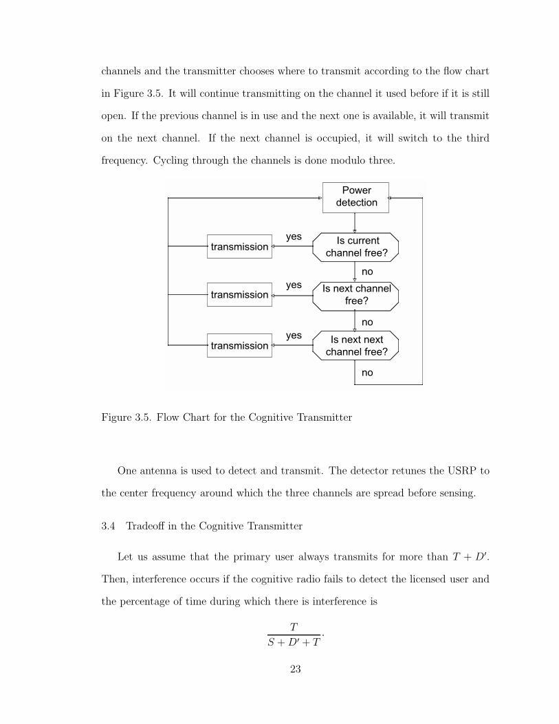
channels and the transmitter chooses where to transmit according to the flow chart

in Figure 3.5. It will continue transmitting on the channel it used before if it is still

open. If the previous channel is in use and the next one is available, it will transmit

on the next channel. If the next channel is occupied, it will switch to the third

frequency. Cycling through the channels is done modulo three.

Figure 3.5. Flow Chart for the Cognitive Transmitter

One antenna is used to detect and transmit. The detector retunes the USRP to

the center frequency around which the three channels are spread before sensing.

3.4 Tradeoff in the Cognitive Transmitter

Let us assume that the primary user always transmits for more than T + D′.

Then, interference occurs if the cognitive radio fails to detect the licensed user and

the percentage of time during which there is interference is

T

S + D′ + T·

23

The probability of missed detection is 1 − Pd so the maximum percentage of time

during which the primary and secondary users interfere is

(1 − Pd)T

S + D′ + T· (3.1)

On the other hand, the cognitive radio wants to transmit as much data as possible.

The probability that the transmitter decides that a primary user is present while

in fact it is not is Pf . In that case, the cognitive radio will miss its chance to

transmit. Hence, the percent of time during which the cognitive radio transmits

when a channel is available is

(1 − Pf)T

S + D′ + T(3.2)

and the effective bit rate of transmission is

R(1 − Pf)T

S + D′ + T

with R the nominal bit rate, 500 kbits/s. There is a tradeoff between quantities

(3.1) and (3.2). The interference time must be minimized, which implies a small

value for T and a large value for S. However, to maximize the effective bit rate, T

should be large and S small.

In our implementation, there is the following constraint on T , S and D′:

R(1 − Pf )T

S + D′ + T> Rmusic (3.3)

Rmusic is the rate of the music transmitted by the cognitive transmitter to the

receiver. The original music at 44,100 samples/s has been downsampled by a factor

of 4 in order to be transmitted by the cognitive radio. The sample size is 16 bits so

the rate of the mono music is 176.4 kbits/s.

D′, the delay due to hardware latency, does not depend on T . Table 3.1 shows

24

that the probability of detecting that the channels are in use while in fact they are

not (Pf) depends on D, the time during which the detector discards samples. This

Pf is not linked to the primary user detection. The smaller D, the larger Pf because

a small D implies that the detector senses the channels while transmission is still on.

These results are obtained at high SNR (high threshold) so that Pf only depends

on D. T is equal to 97 ms and S is 10 ms. The number of trials is 10,000.

TABLE 3.1

RELATIONSHIP BETWEEN D AND Pf

D, discard time Pf , probability of false alarm115 ms 0.9 %120 ms 0.3 %125 ms 0.03 %130 ms 0 %

For our implementation, we choose to take D =125 ms so that the cognitive trans-

mitter does not change channel without reason (Pf=0.03 %). T is chosen to be equal

to 97 ms so that we obtain a good audio quality and S is chosen to be equal to 10

ms. These values satisfy constraint (3.3); the effective bit rate of transmission is

359.3 kbits/s. We choose this bit rate so that there is no interruption in the music

when frequency is changed and frequency switching is essentially unnoticeable to

the end user. However, practically, the effective bit rate should be chosen close to

the music rate for efficiency.

3.5 Implementation of the Transmitter

This section describes the different signal processing blocks used in the trans-

mitter. The cognitive transmitter sends some packets during T before sensing the

25

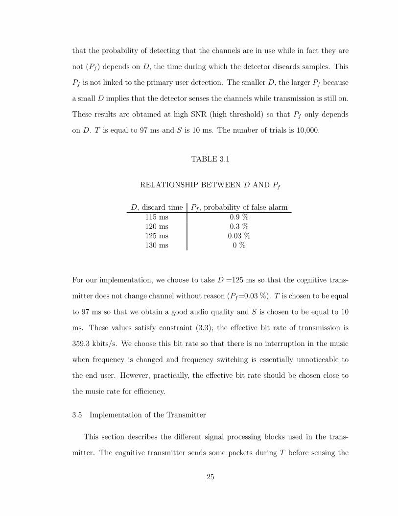
channels again. A packet in GNU Radio consists of a payload (user data), an access

code and a header (length of payload and Cyclic Redundancy Check (CRC)). The

access code is used to identify the beginning of a frame. Figure 3.6 shows the format

of the packet used in our implementation.a c c e s s c o d e C R C 3 2p a y l o a dl e n g t h o fp a y l o a d< = 6 4 b i t s 1 2 8 b i t s 3 2 b i t sFigure 3.6. Format of a Packet

The length of the payload must be between 0 and 4,096 bytes. Experimentally, we

observe that if the cognitive transmitter sends packets of small size (for example,

when the length of the payload is 196 bytes), we can hear extra high frequencies

when the receiver outputs the transmitted music on the speaker. The speaker turns

on when a packet is received and off when the playing of the packet is done. If the

size of the packet is small, the speaker will turn on and off often. For better audio

quality, packets of long size are preferred. The length of the payload is chosen to be

1,996 bytes, the size of the packets is then 16,192 bits (2,024 bytes).

The flow graph of the transmitter part of the cognitive radio is represented in

Figure 3.7. Packetization is done in the flow graph via messages. In GNU Radio,

if you do not want a block to output a sample every time it receives one, you can

use the message architecture. In the flow graph of the transmitter, pkt input is a

message source. The cognitive transmitter sends a packet by calling the function

send pkt of packet transmitter and the following actions are taken:

• make a packet from the payload (add access code and CRC-32)

26

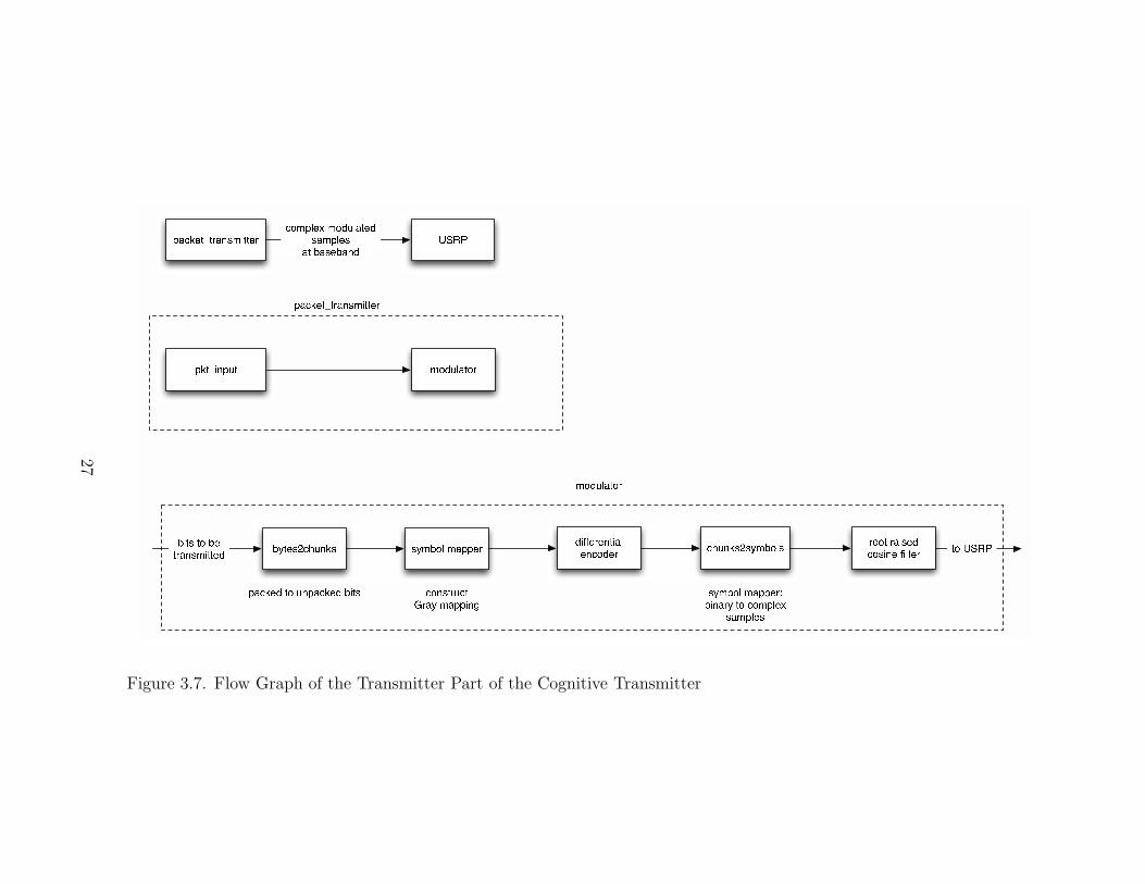
p a c ke t_ tr a n s m i t t e r U S R Pc o m p l e x m o du l a t e ds a m p l e sa t b a s e b a n dby t e s 2 c hu n k s sy m b o l m a p p e r d i f fe r e n t i a le n c o d e r c hu n k s 2 sy m b o l s r o o t r a i s e dc o s i n e fi l t e rsy m b o l m a p p e r :b i n ar y t o c o m p l e xs a m p l e sp a c ke d t o u n p a c ke d b i t sb i t s t o b etr a n s m i t t e d t o U S R Pc o n s tr u c tG r ay m a p p i n g

p k t_ i n pu t m o du l a t o rp a c ke t_ tr a n s m i t t e r

m o du l a t o rFigure 3.7. Flow Graph of the Transmitter Part of the Cognitive Transmitter

27

• make a message from the packet

• insert message into the message queue of pkt input

Messages are sent from pkt input to modulator. In the modulator, samples are

DBPSK-modulated. Differential modulation is preferred because it is easier to im-

plement. It does not require to derotate the samples at the receiver. The input

stream coming into the modulator is made of bytes (data are grouped in 8 bits);

the block bytes2chunks regroups the bytes into k-bits vectors with k the number of

bits per symbol (for DBPSK, k is 1; for DQPSK, k is 2). symbol mapper Gray-maps

the incoming chunks of 2 bits:

00 → 00

01 → 01

10 → 11

11 → 10

The differential encoder for DBPSK modulation performs the following operation:

yi = yi−1 ⊕ xi

where yi is the actual transmitted bit, xi the bit to be transmitted and ⊕ is the

modulo-2 addition.

For DQPSK, we have the following relationship between bits and difference in

phase:

0◦ → 00

90◦ → 01

180◦ → 11

−90◦ → 10

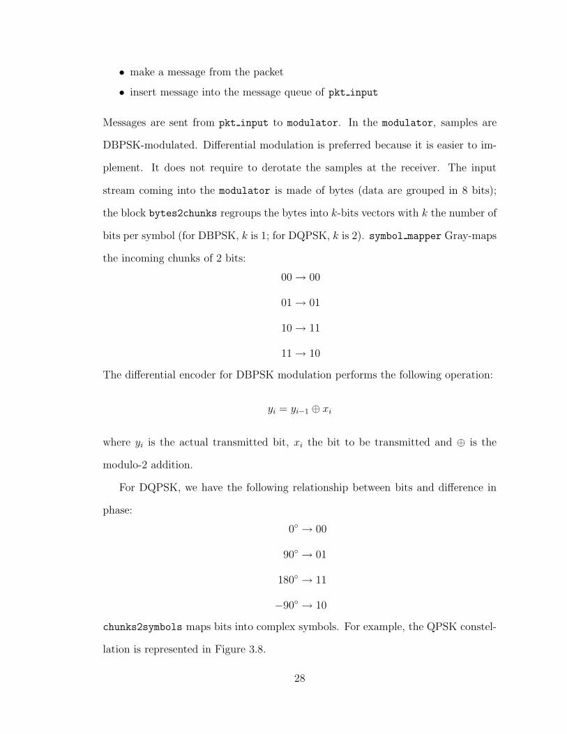
chunks2symbols maps bits into complex symbols. For example, the QPSK constel-

lation is represented in Figure 3.8.

28

0 1 0 01 1 1 0Figure 3.8. QPSK Constellation with Gray-Mapping

Finally, the complex symbols are passed through a Root-Raised Cosine (RRC) pulse-

shaping filter. Throughout this work, the DBPSK modulation is used with a symbol

and bit rate of 500 kbits/s.

3.6 Power Detector

3.6.1 Implementation

We will now study in more detail how the detector in Figure 3.4 works. Figure 3.9

shows the different signal processing blocks present in the detector. The block s2v

takes a stream of complex samples and turns them into a stream of complex vectors.

Vectors are of size fft size (denoted as Q). Samples are then multiplied by a

Blackman-Harris window before the FFT. c2mag computes the squared magnitude

of the FFT samples. After fft correction, an estimate of the Power Spectral

Density (PSD) is obtained (averaged periodogram):

P (i) =1

M

1

Q

M−1∑

k=0

∣

∣

∣

∣

∣

Q−1∑

n=0

y(n + kQ) exp

(

−2πji

Qn

)

∣

∣

∣

∣

∣

2

where y is the complex baseband signal (non demodulated), Q is the size of FFT

(4,096) and M is the number of non overlapping PSD frames averaged (10):

M =Sfs

Q

29

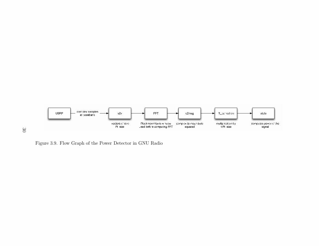
U S R P s 2v F F T c 2 m a g f f t_ c o r r e c t i o n s t a t sc o m p l e x s a m p l e sa t b a s e b a n d B l a c k m a n� H a r r i s w i n d o wu s e d b e f o r e c o m p u t i n g F F Tv e c t o r s o f s iz ef f t_ s iz e c o m p l e x t o m a g n i t u d es q u a r e d m u l t i p l i c a t i o n by1 / f f t_ s iz e c o m p u t e s p o w e r o f t h es i g n a l

Figure 3.9. Flow Graph of the Power Detector in GNU Radio

30

fs is the sampling frequency of the samples coming from the FPGA (4 MHz) and S

is the sensing time (10 ms). The detector’s cycle represented in Figure 3.4 (Sensing-

Discard-Sensing-Discard...) is done inside the C++ block stats. The steps followed

in this block are:

1. Retune the USRP to the center frequency around which the three channelsare spread

2. Discard samples from the USRP for a duration of tune delay (D)

3. Compute time average of the PSD samples for a duration of dwell delay (S)

4. Calculate the powers on the three channels by summing the PSD points andthen decide if the channel is open or in use by comparing the calculated powerto a threshold

5. Send the result to the transmitter

In the implementation, a double-sided bandwidth of 4 MHz is sensed. In this band,

three channels (1 MHz wide) are considered. To calculate the power on one channel

(Pchannel), the PSD points belonging to the channel are summed:

Pchannel =∑

i∈channel

P (i) (3.4)

The number of PSD samples summed in each channel is 1,024. For example, if the

center frequency of the USRP is 434 MHz, the following points are summed in the

three channels:

• channel 1: [432.5-433.5 MHz], i = 2560 → 3583

• channel 2: [433.5-434.5 MHz], i = 0 → 511, 3584 → 4095

• channel 3: [434.5-435.5 MHz], i = 512 → 1535

As discussed in Section 2.3.3, the power detector must decide between two hy-

potheses:

H0 : primary user not present

HS : primary user present

31

The decision rule is the following:

Pchannel

HS

≷H0

γ

where γ is a threshold.

3.6.2 Performance

Figure 3.10 shows the experimental ROCs obtained for the power detector de-

scribed in the previous section.

0 0.1 0.2 0.3 0.4 0.5 0.6 0.7 0.8 0.9 10

0.1

0.2

0.3

0.4

0.5

0.6

0.7

0.8

0.9

1

Pf

Pd

ROC curve

SNR=−13 dBSNR=−15 dBSNR=−16 dBSNR=−17 dBSNR=−19dBSNR=−21dBSNR=−23 dB

Figure 3.10. Receiver Operating Characteristic for the Power Detector

To obtain this plot, one USRP served as the detector and the other one sent DBPSK

signals at different amplitudes, i.e., the parameter tx amplitude of the transmitter

is varied. The conditions in which these ROC plots have been taken are:

• The PSD points are averaged over dwell delay=S=0.04 sec

32

• The calculated power is the one in a channel of 1 MHz bandwidth with centerfrequency equal to 435 MHz.

• The USRPs are placed in an indoor environment, one meter apart.

The parameter for this ROC curve is the SNRdB :

SNRdB = 10 log10

Psignal+noise − Pnoise

Pnoise

Psignal+noise and Pnoise are given by the block stats, they are calculated according

to (3.4). This assumed that the signal and the noise are independent:

Psignal+noise = Psignal + Pnoise

The difficulty in plotting the ROC is the fact that we are estimating the (Pd,Pf )

curve. For finite sample size, it can happen that when the threshold is increased,

the estimated probability of false alarm does not necessarily decrease, even if the

probability is calculated over 1,000 trials and the sensing time S is 0.04 sec. The

idea is then to average the probabilities of false alarm for a same threshold over time.

Hence, Figure 3.10 is obtained by counting how many times we detect a signal in

1,000 trials; we do this at four different times and then average the probabilities.

The fact that Pf does not necessarily decrease when the threshold is increased can

be explained in several ways. One explanation is that the number of trials or the

sensing time S are not large enough, and another explanation is that the noise and

interference are non stationary.

According to the ROC, we have essentially ideal detection (Pd = 1 and Pf=0)

(at least over 4,000 trials) for SNRs greater than -13 dB when the number of PSD

samples N summed in the channel is 1,024 and the sensing time S is 0.04 s. If N

is less than 1,024, then the detector will perform poorer (smaller Pd and Pf) for

the same SNR of -13 dB. Performance of the power detector not only depends on

33

the SNR, but also on the number of samples used for detection N . As formula

2.2 shows, for the same Pd and Pf , a smaller SNR requires a larger N . Similarly,

performance of the power detector also depends on S. A smaller S means a less

accurate estimate of the power in the channel and hence smaller Pd and Pf for a

same SNR and N .

If Pf is specified and the SNR is known, the ROC will give the threshold corre-

sponding to the desired Pf . In our demonstration with the PTT handheld device,

the value of the power of the noise calculated according to formula (3.4) is around

300,000 and the power of the signal sent by the PTT device is 1,000 times larger.

The value of the threshold is chosen to be 5,000,000. The number 300,000 is ob-

tained when S=0.01 sec and the bandwidth of the channel is 1 MHz with center

frequency of 434 MHz. The PTT is placed one meter away from the detector.

3.7 List of the Programs used in the Cognitive Transmitter

Table 3.2 gives the list of the programs used for the implementation of the

cognitive transmitter.

TABLE 3.2

PROGRAMS USED IN THE COGNITIVE TRANSMITTER

File Name Descriptioncognitive transmitter.py contains the flow graph in Figure 3.9foo syms to bytes 2.cc stats block, computes power of the channelsfoo syms to bytes 2.h declaration of variables used in foo syms to bytes 2.cc

transmit path.py contains the flow graph in Figure 3.7form alice.py builds the components necessary for the GUIstdgui3.py builds the components necessary for the GUI

34

CHAPTER 4

COGNITIVE RECEIVER

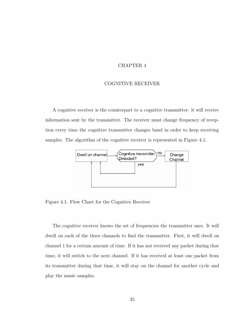
A cognitive receiver is the counterpart to a cognitive transmitter: it will receive

information sent by the transmitter. The receiver must change frequency of recep-

tion every time the cognitive transmitter changes band in order to keep receiving

samples. The algorithm of the cognitive receiver is represented in Figure 4.1.D w e l l o n c h a n n e l C o g n i t i v e t r a n s m i t t e rD e t e c t e d ? C h a n g eC h a n n e ly e s n oFigure 4.1. Flow Chart for the Cognitive Receiver

The cognitive receiver knows the set of frequencies the transmitter uses. It will

dwell on each of the three channels to find the transmitter. First, it will dwell on

channel 1 for a certain amount of time. If it has not received any packet during that

time, it will switch to the next channel. If it has received at least one packet from

its transmitter during that time, it will stay on the channel for another cycle and

play the music samples.

35

4.1 Synchronization between Cognitive Transmitter and Receiver

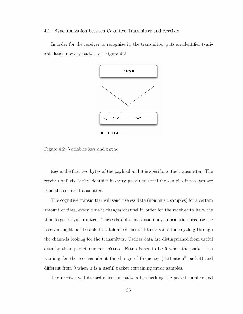
In order for the receiver to recognize it, the transmitter puts an identifier (vari-

able key) in every packet, cf. Figure 4.2.p a y l o a dk e y p k t n o d a t a1 6 b i t s 1 6 b i t s

Figure 4.2. Variables key and pktno

key is the first two bytes of the payload and it is specific to the transmitter. The

receiver will check the identifier in every packet to see if the samples it receives are

from the correct transmitter.

The cognitive transmitter will send useless data (non music samples) for a certain

amount of time, every time it changes channel in order for the receiver to have the

time to get resynchronized. These data do not contain any information because the

receiver might not be able to catch all of them: it takes some time cycling through

the channels looking for the transmitter. Useless data are distinguished from useful

data by their packet number, pktno. Pktno is set to be 0 when the packet is a

warning for the receiver about the change of frequency (“attention” packet) and

different from 0 when it is a useful packet containing music samples.

The receiver will discard attention packets by checking the packet number and

36

play music packets (pktno different from 0) on the speaker.

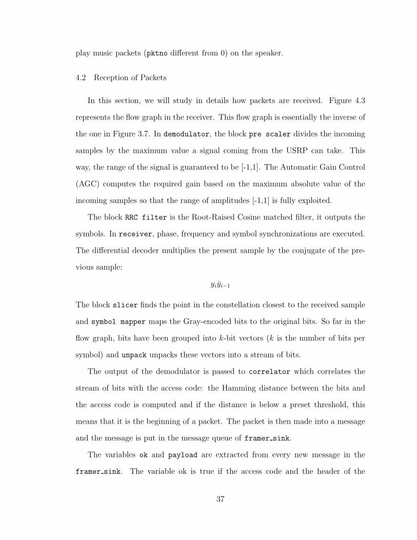
4.2 Reception of Packets

In this section, we will study in details how packets are received. Figure 4.3

represents the flow graph in the receiver. This flow graph is essentially the inverse of

the one in Figure 3.7. In demodulator, the block pre scaler divides the incoming

samples by the maximum value a signal coming from the USRP can take. This

way, the range of the signal is guaranteed to be [-1,1]. The Automatic Gain Control

(AGC) computes the required gain based on the maximum absolute value of the

incoming samples so that the range of amplitudes [-1,1] is fully exploited.

The block RRC filter is the Root-Raised Cosine matched filter, it outputs the

symbols. In receiver, phase, frequency and symbol synchronizations are executed.

The differential decoder multiplies the present sample by the conjugate of the pre-

vious sample:

yiyi−1

The block slicer finds the point in the constellation closest to the received sample

and symbol mapper maps the Gray-encoded bits to the original bits. So far in the

flow graph, bits have been grouped into k-bit vectors (k is the number of bits per

symbol) and unpack unpacks these vectors into a stream of bits.

The output of the demodulator is passed to correlator which correlates the

stream of bits with the access code: the Hamming distance between the bits and

the access code is computed and if the distance is below a preset threshold, this

means that it is the beginning of a packet. The packet is then made into a message

and the message is put in the message queue of framer sink.

The variables ok and payload are extracted from every new message in the

framer sink. The variable ok is true if the access code and the header of the

37

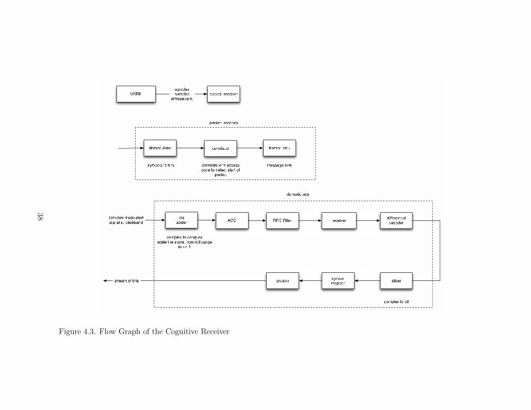
U S R P p a c ke t_ re ce iv e r

d e m o du l a t o r c o r re l a t o r f r a m e r_ s in ks y m b o l s t o b i t s c o r re l a t e w i t h a c ce s sc o d e t o d e t e c t s t a r t o fp a c ke t m e s s a g e s in k

c o m p l e xs a m p l e sa t b a s e b an dp res c a l e r A G C R R C F i l t e r re ce iv e r d i f fe re n t i a ld e c o d e rc o m p l e x t o c o m p l e xs c a l e t h e s i g n a l f r o m fu l l r an g et o + /" 1c o m p l e x m o d u l a t e ds i gn a l a t b a s e b an d

s l i ce rs y m b o lm a p p e r c o m p l e x t o b i tu n p a c ks t re a m o f b i t sp a c ke t _ re ce iv e r

d e m o du l a t o r

Figure 4.3. Flow Graph of the Cognitive Receiver

38

packet (length of payload and CRC) are correctly decoded. It is false if the CRC is

false: the packet has been corrupted. payload is generated by removing the access

code and header from the packet. The function rx callback enables the main loop

to have access to ok and payload.

4.3 Playing of Music

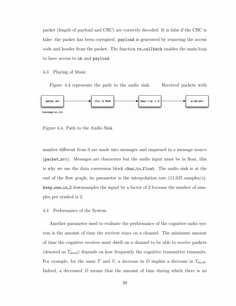
Figure 4.4 represents the path to the audio sink. Received packets withp a c k e t _ s r c c h a r _ t o _ fl o a t k e e p _ o n e _ i n _ 2 a u d i o . s i n km e s s a g e s o u r c eFigure 4.4. Path to the Audio Sink

number different from 0 are made into messages and enqueued in a message source

(packet src). Messages are characters but the audio input must be in float, this

is why we use the data conversion block char to float. The audio sink is at the

end of the flow graph, its parameter is the interpolation rate (11,025 samples/s).

keep one in 2 downsamples the signal by a factor of 2 because the number of sam-

ples per symbol is 2.

4.4 Performance of the System

Another parameter used to evaluate the performance of the cognitive radio sys-

tem is the amount of time the receiver stays on a channel. The minimum amount

of time the cognitive receiver must dwell on a channel to be able to receive packets

(denoted as Tdwell) depends on how frequently the cognitive transmitter transmits.

For example, for the same T and S, a decrease in D implies a decrease in Tdwell.

Indeed, a decreased D means that the amount of time during which there is no

39

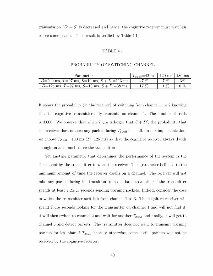
transmission (D′ + S) is decreased and hence, the cognitive receiver must wait less

to see some packets. This result is verified by Table 4.1.

TABLE 4.1

PROBABILITY OF SWITCHING CHANNEL

Parameters Tdwell=42 ms 120 ms 180 msD=200 ms, T=97 ms, S=10 ms, S + D′=113 ms 47 % 7 % 3%D=125 ms, T=97 ms, S=10 ms, S + D′=38 ms 17 % 1 % 0 %

It shows the probability (at the receiver) of switching from channel 1 to 2 knowing

that the cognitive transmitter only transmits on channel 1. The number of trials

is 3,000. We observe that when Tdwell is larger that S + D′, the probability that

the receiver does not see any packet during Tdwell is small. In our implementation,

we choose Tdwell =180 ms (D=125 ms) so that the cognitive receiver always dwells

enough on a channel to see the transmitter.

Yet another parameter that determines the performance of the system is the

time spent by the transmitter to warn the receiver. This parameter is linked to the

minimum amount of time the receiver dwells on a channel. The receiver will not

miss any packet during the transition from one band to another if the transmitter

spends at least 2 Tdwell seconds sending warning packets. Indeed, consider the case

in which the transmitter switches from channel 1 to 3. The cognitive receiver will

spend Tdwell seconds looking for the transmitter on channel 1 and will not find it,

it will then switch to channel 2 and wait for another Tdwell and finally, it will get to

channel 3 and detect packets. The transmitter does not want to transmit warning

packets for less than 2 Tdwell because otherwise, some useful packets will not be

received by the cognitive receiver.

40

In our implementation, Tdwell is 180 ms so the cognitive transmitter must send

warning packets for at least 360 ms. The number of times (denoted as counter)

the sequence “Sense-Discard-Sense-Discard” must be repeated at the transmitter to

warn the receiver is at least 3 ( (125+10)*3=405 ms > 360 ms). To be on the safe

side, we choose to repeat this sequence 5 times so the cognitive transmitter senses

and sends warning packets for 135*5=675 ms.

Table 4.2 gives the values of the parameters used in the implemented cognitive

radio system. When switching from one channel to another, the transmitter sends

TABLE 4.2

PARAMETERS OF THE COGNITIVE RADIO SYSTEM

Parameter ValueS 10 msT 97 ms if music packet, 11 ms if warning packetD′ 28 msD 125 ms

Tdwell 180 mscounter 5

L, length of packet 1,996 bytes if music packet, 150 bytes if warning packet

warning packets for 11 ms and does not do anything for S + D′=124 ms which is

less than the time the cognitive receiver dwells on a frequency (180 ms). Hence, the

receiver is able to receive the warning packets and it can get resynchronized when

the frequency of transmission is changed.

4.5 List of the Programs used in the Cognitive Receiver

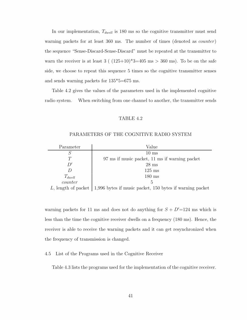
Table 4.3 lists the programs used for the implementation of the cognitive receiver.

41

TABLE 4.3

PROGRAMS USED IN THE COGNITIVE RECEIVER

File Name Descriptioncognitive receiver.py implements the algorithm in Figure 4.1

receive path.py contains the flow graph in Figure 4.3

4.6 Cognitive Radio Network

The implemented cognitive transmitter and receiver can be part of a network

comprised of several cognitive systems and a collection of primary users. The cog-

nitive systems and the primary users coexist on the same channels. Each cognitive

radio avoids both the primary users and the other cognitive radios because of the

detection based on power. A cognitive receiver will not play the music samples

coming from other transmitters because of the identifier.

If the primary user occupies one channel, the cognitive radios will occupy the

other two channels. But if the primary users transmit on two channels, one cognitive

radio will transmit on the third channel while other cognitive radios will not transmit

at all: in the current implementation, the secondary users do not share the available

spectrum.

Figure 4.5 shows a spectrum analyzer result for two cognitive transmitters trans-

mitting at 433 and 434 MHz and one primary user (PTT handheld device) trans-

mitting at 435 MHz.

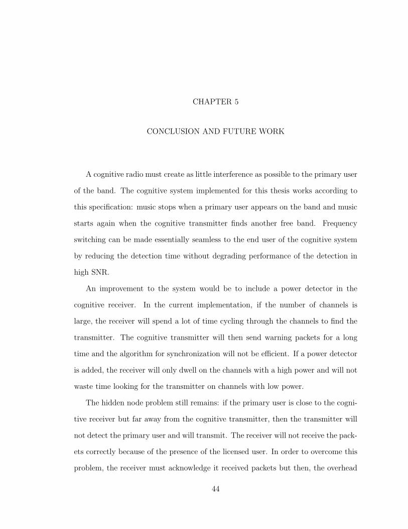
Figure 4.6 shows a spectrum analyzer result for two primary users at 434 and

435 MHz and one cognitive radio transmitting at 433 MHz.

42

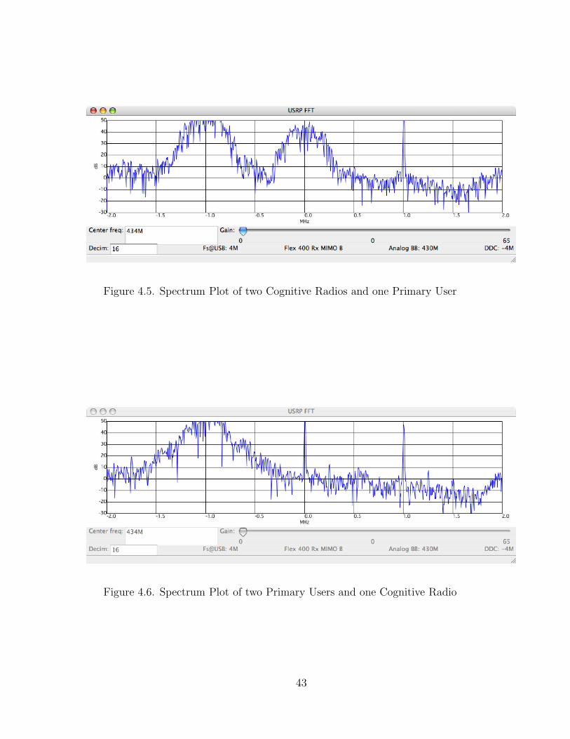
Figure 4.5. Spectrum Plot of two Cognitive Radios and one Primary User

Figure 4.6. Spectrum Plot of two Primary Users and one Cognitive Radio

43

CHAPTER 5

CONCLUSION AND FUTURE WORK

A cognitive radio must create as little interference as possible to the primary user

of the band. The cognitive system implemented for this thesis works according to

this specification: music stops when a primary user appears on the band and music

starts again when the cognitive transmitter finds another free band. Frequency

switching can be made essentially seamless to the end user of the cognitive system

by reducing the detection time without degrading performance of the detection in

high SNR.

An improvement to the system would be to include a power detector in the

cognitive receiver. In the current implementation, if the number of channels is

large, the receiver will spend a lot of time cycling through the channels to find the

transmitter. The cognitive transmitter will then send warning packets for a long

time and the algorithm for synchronization will not be efficient. If a power detector

is added, the receiver will only dwell on the channels with a high power and will not

waste time looking for the transmitter on channels with low power.

The hidden node problem still remains: if the primary user is close to the cogni-

tive receiver but far away from the cognitive transmitter, then the transmitter will

not detect the primary user and will transmit. The receiver will not receive the pack-

ets correctly because of the presence of the licensed user. In order to overcome this

problem, the receiver must acknowledge it received packets but then, the overhead

44

is increased. Cooperative sensing is also a potential solution to this problem.

OFDM should ideally be used in the cognitive transmitter instead of DBPSK

because the bandwidth occupied by this transmission can be changed dynamically

to match the available bandwidth.

45

BIBLIOGRAPHY

[1] I. Akyildiz, W. Lee, M. Vuran, and S. Mohanty. NeXt generation/dynamicspectrum access/cognitive radio wireless networks: A survey. Computer Net-works, 50(13):2127–2159, 2006.

[2] D. Cabric, S. Mishra, and R. Brodersen. Implementation Issues in SpectrumSensing for Cognitive Radios. Conference Record on the Thirty-Eighth AsilomarConference on Signals, Systems and Computers, 1:772–776, 2004.

[3] D. Cabric, A. Tkachenko, and R. Brodersen. Experimental Study of SpectrumSensing based on Energy Detection and Network Cooperation. ACM 1st Inter-national Workshop on Technology and Policy for Accessing Spectrum (TAPAS),2006.

[4] C.R.C. da Silva, B. Choi, and K. Kim. Distributed Spectrum Sensing forCognitive Radio Systems. Information Theory and Applications Workshop,pages 120–123, 2007.

[5] F. Digham, M. Alouini, and M. Simon. On the Energy Detection of UnknownSignals over Fading Channels. IEEE International Conference on Communica-tions, 5:3575–3579, 2003.

[6] G. Ganesan and Y. Li. Agility Improvement through Cooperative Diversity inCognitive Radio. IEEE Global Telecommunications Conference, 5, 2005.

[7] A. Ghasemi and E. Sousa. Collaborative Spectrum Sensing for OpportunisticAccess in Fading Environments. First IEEE International Symposium on NewFrontiers in Dynamic Spectrum Access Networks, pages 131–136, 2005.

[8] M. Haddad, M. Debbah, and A. Menouni Hayar. On Achievable Performance ofCognitive Radio Systems. IEEE Journal on Selected Areas in Communications”Cognitive Radio: Theory and Applications”, 2007.

[9] S. Haykin. Cognitive Radio: Brain-Empowered Wireless Communications.IEEE journal on selected areas in communications, 23(2), February 2005.

[10] J. Hillenbrand, T. Weiss, and F. Jondral. Calculation of Detection and FalseAlarm Probabilities in Spectrum Pooling Systems. IEEE Communications Let-ters, 9:349–351, 2005.

[11] B. Horine and D. Turgut. Link Rendezvous Protocol for Cognitive Radio Net-works. 2nd IEEE International Symposium on New Frontiers in Dynamic Spec-trum Access Networks, pages 444–447, 2007.

46

[12] T. O’Shea, T. Clancy, and H. Ebeid. Practical Signal Detection and Classifi-cation in GNU Radio. 2007 Software Defined Radio Technical Conference andProduct Exposition.

[13] A. Sahai, N. Hoven, and R. Tandra. Some Fundamental Limits on CognitiveRadio. Allerton Conference on Communication, Control and Computing, 2004.

[14] P. Sutton, K. Nolan, and L. Doyle. Cyclostationary Signatures in PracticalCognitive Radio Applications. IEEE Journal on Selected Areas in Communi-cations, 26:13–24, 2008.

47