Practical Animation of Compressible Flow for Shock - PhysBAM

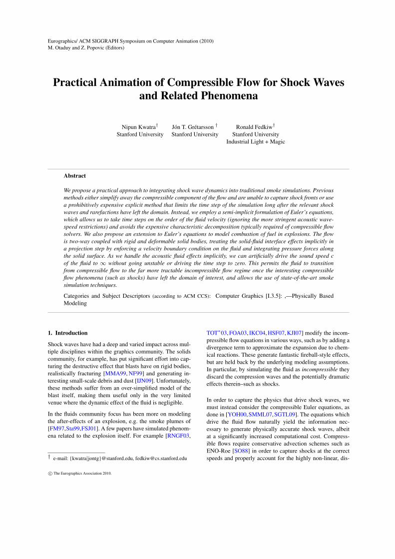
Eurographics/ ACM SIGGRAPH Symposium on Computer Animation (2010)M. Otaduy and Z. Popovic (Editors)

Practical Animation of Compressible Flow for Shock Wavesand Related Phenomena

Nipun Kwatra† Jón T. Grétarsson † Ronald Fedkiw†

Stanford University Stanford University Stanford UniversityIndustrial Light + Magic

Abstract

We propose a practical approach to integrating shock wave dynamics into traditional smoke simulations. Previousmethods either simplify away the compressible component of the flow and are unable to capture shock fronts or usea prohibitively expensive explicit method that limits the time step of the simulation long after the relevant shockwaves and rarefactions have left the domain. Instead, we employ a semi-implicit formulation of Euler’s equations,which allows us to take time steps on the order of the fluid velocity (ignoring the more stringent acoustic wave-speed restrictions) and avoids the expensive characteristic decomposition typically required of compressible flowsolvers. We also propose an extension to Euler’s equations to model combustion of fuel in explosions. The flowis two-way coupled with rigid and deformable solid bodies, treating the solid-fluid interface effects implicitly ina projection step by enforcing a velocity boundary condition on the fluid and integrating pressure forces alongthe solid surface. As we handle the acoustic fluid effects implicitly, we can artificially drive the sound speed cof the fluid to ∞ without going unstable or driving the time step to zero. This permits the fluid to transitionfrom compressible flow to the far more tractable incompressible flow regime once the interesting compressibleflow phenomena (such as shocks) have left the domain of interest, and allows the use of state-of-the-art smokesimulation techniques.

Categories and Subject Descriptors (according to ACM CCS): Computer Graphics [I.3.5]: ,—Physically BasedModeling

1. Introduction

Shock waves have had a deep and varied impact across mul-tiple disciplines within the graphics community. The solidscommunity, for example, has put significant effort into cap-turing the destructive effect that blasts have on rigid bodies,realistically fracturing [MMA99, NF99] and generating in-teresting small-scale debris and dust [IJN09]. Unfortunately,these methods suffer from an over-simplified model of theblast itself, making them useful only in the very limitedvenue where the dynamic effect of the fluid is negligible.

In the fluids community focus has been more on modelingthe after-effects of an explosion, e.g. the smoke plumes of[FM97,Sta99,FSJ01]. A few papers have simulated phenom-ena related to the explosion itself. For example [RNGF03,

† e-mail: {kwatra|jontg}@stanford.edu, [email protected]

TOT∗03, FOA03, IKC04, HSF07, KJI07] modify the incom-pressible flow equations in various ways, such as by adding adivergence term to approximate the expansion due to chem-ical reactions. These generate fantastic fireball-style effects,but are held back by the underlying modeling assumptions.In particular, by simulating the fluid as incompressible theydiscard the compression waves and the potentially dramaticeffects therein–such as shocks.

In order to capture the physics that drive shock waves, wemust instead consider the compressible Euler equations, asdone in [YOH00,SMML07,SGTL09]. The equations whichdrive the fluid flow naturally yield the information nec-essary to generate physically accurate shock waves, albeitat a significantly increased computational cost. Compress-ible flows require conservative advection schemes such asENO-Roe [SO88] in order to capture shocks at the correctspeeds and properly account for the highly non-linear, dis-

c© The Eurographics Association 2010.

kwatra et al. / Practical Animation of Compressible Flow for Shock Waves and Related Phenomena

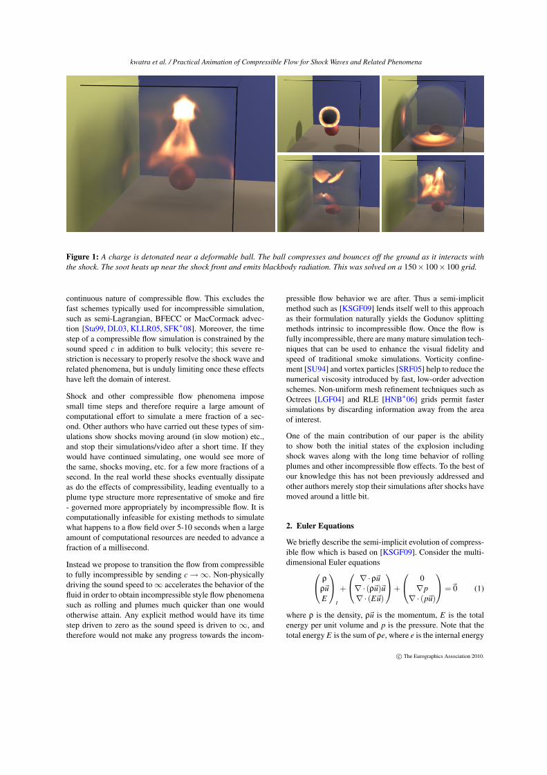
Figure 1: A charge is detonated near a deformable ball. The ball compresses and bounces off the ground as it interacts withthe shock. The soot heats up near the shock front and emits blackbody radiation. This was solved on a 150×100×100 grid.

continuous nature of compressible flow. This excludes thefast schemes typically used for incompressible simulation,such as semi-Lagrangian, BFECC or MacCormack advec-tion [Sta99, DL03, KLLR05, SFK∗08]. Moreover, the timestep of a compressible flow simulation is constrained by thesound speed c in addition to bulk velocity; this severe re-striction is necessary to properly resolve the shock wave andrelated phenomena, but is unduly limiting once these effectshave left the domain of interest.

Shock and other compressible flow phenomena imposesmall time steps and therefore require a large amount ofcomputational effort to simulate a mere fraction of a sec-ond. Other authors who have carried out these types of sim-ulations show shocks moving around (in slow motion) etc.,and stop their simulations/video after a short time. If theywould have continued simulating, one would see more ofthe same, shocks moving, etc. for a few more fractions of asecond. In the real world these shocks eventually dissipateas do the effects of compressibility, leading eventually to aplume type structure more representative of smoke and fire- governed more appropriately by incompressible flow. It iscomputationally infeasible for existing methods to simulatewhat happens to a flow field over 5-10 seconds when a largeamount of computational resources are needed to advance afraction of a millisecond.

Instead we propose to transition the flow from compressibleto fully incompressible by sending c →∞. Non-physicallydriving the sound speed to∞ accelerates the behavior of thefluid in order to obtain incompressible style flow phenomenasuch as rolling and plumes much quicker than one wouldotherwise attain. Any explicit method would have its timestep driven to zero as the sound speed is driven to ∞, andtherefore would not make any progress towards the incom-

pressible flow behavior we are after. Thus a semi-implicitmethod such as [KSGF09] lends itself well to this approachas their formulation naturally yields the Godunov splittingmethods intrinsic to incompressible flow. Once the flow isfully incompressible, there are many mature simulation tech-niques that can be used to enhance the visual fidelity andspeed of traditional smoke simulations. Vorticity confine-ment [SU94] and vortex particles [SRF05] help to reduce thenumerical viscosity introduced by fast, low-order advectionschemes. Non-uniform mesh refinement techniques such asOctrees [LGF04] and RLE [HNB∗06] grids permit fastersimulations by discarding information away from the areaof interest.

One of the main contribution of our paper is the abilityto show both the initial states of the explosion includingshock waves along with the long time behavior of rollingplumes and other incompressible flow effects. To the best ofour knowledge this has not been previously addressed andother authors merely stop their simulations after shocks havemoved around a little bit.

2. Euler Equations

We briefly describe the semi-implicit evolution of compress-ible flow which is based on [KSGF09]. Consider the multi-dimensional Euler equations ρ

ρ~uE

t

+

∇·ρ~u∇· (ρ~u)~u∇· (E~u)

+

0∇p

∇· (p~u)

=~0 (1)

where ρ is the density, ρ~u is the momentum, E is the totalenergy per unit volume and p is the pressure. Note that thetotal energy E is the sum of ρe, where e is the internal energy



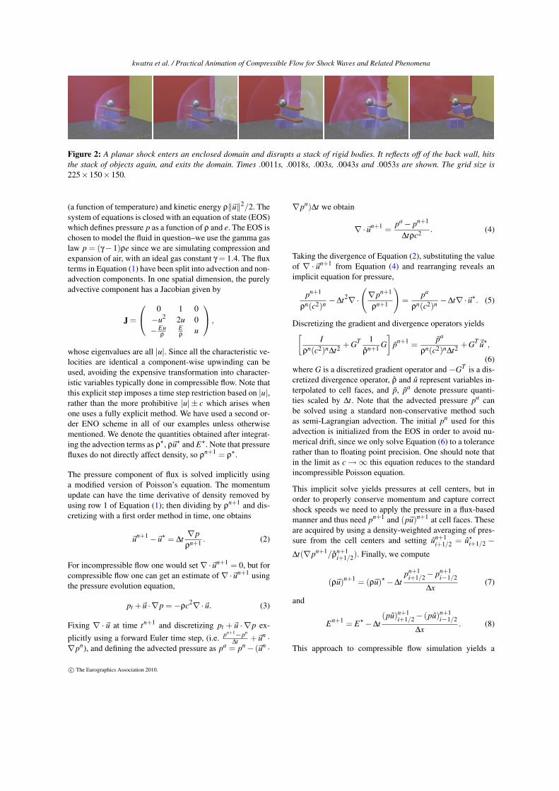
Figure 2: A planar shock enters an enclosed domain and disrupts a stack of rigid bodies. It reflects off of the back wall, hitsthe stack of objects again, and exits the domain. Times .0011s, .0018s, .003s, .0043s and .0053s are shown. The grid size is225×150×150.

(a function of temperature) and kinetic energy ρ‖~u‖2/2. Thesystem of equations is closed with an equation of state (EOS)which defines pressure p as a function of ρ and e. The EOS ischosen to model the fluid in question–we use the gamma gaslaw p = (γ−1)ρe since we are simulating compression andexpansion of air, with an ideal gas constant γ = 1.4. The fluxterms in Equation (1) have been split into advection and non-advection components. In one spatial dimension, the purelyadvective component has a Jacobian given by

J =

0 1 0−u2 2u 0−Eu

ρ

Eρ

u

,

whose eigenvalues are all |u|. Since all the characteristic ve-locities are identical a component-wise upwinding can beused, avoiding the expensive transformation into character-istic variables typically done in compressible flow. Note thatthis explicit step imposes a time step restriction based on |u|,rather than the more prohibitive |u| ± c which arises whenone uses a fully explicit method. We have used a second or-der ENO scheme in all of our examples unless otherwisementioned. We denote the quantities obtained after integrat-ing the advection terms as ρ

?, ρ~u? and E?. Note that pressurefluxes do not directly affect density, so ρ

n+1 = ρ?.

The pressure component of flux is solved implicitly usinga modified version of Poisson’s equation. The momentumupdate can have the time derivative of density removed byusing row 1 of Equation (1); then dividing by ρ

n+1 and dis-cretizing with a first order method in time, one obtains

~un+1−~u? = ∆t∇p

ρn+1 . (2)

For incompressible flow one would set ∇·~un+1 = 0, but forcompressible flow one can get an estimate of ∇·~un+1 usingthe pressure evolution equation,

pt +~u ·∇p =−ρc2∇·~u. (3)

Fixing ∇ ·~u at time tn+1 and discretizing pt +~u · ∇p ex-plicitly using a forward Euler time step, (i.e. pn+1−pn

∆t +~un ·∇pn), and defining the advected pressure as pa = pn− (~un ·

∇pn)∆t we obtain

∇·~un+1 =pa− pn+1

∆tρc2 . (4)

Taking the divergence of Equation (2), substituting the valueof ∇ ·~un+1 from Equation (4) and rearranging reveals animplicit equation for pressure,

pn+1

ρn(c2)n −∆t2∇·

(∇pn+1

ρn+1

)=

pa

ρn(c2)n −∆t∇·~u?. (5)

Discretizing the gradient and divergence operators yields[I

ρn(c2)n∆t2 +GT 1ρn+1 G

]pn+1 =

pa

ρn(c2)n∆t2 +GT~u?,

(6)where G is a discretized gradient operator and−GT is a dis-cretized divergence operator, ρ and u represent variables in-terpolated to cell faces, and p, pa denote pressure quanti-ties scaled by ∆t. Note that the advected pressure pa canbe solved using a standard non-conservative method suchas semi-Lagrangian advection. The initial pn used for thisadvection is initialized from the EOS in order to avoid nu-merical drift, since we only solve Equation (6) to a tolerancerather than to floating point precision. One should note thatin the limit as c →∞ this equation reduces to the standardincompressible Poisson equation.

This implicit solve yields pressures at cell centers, but inorder to properly conserve momentum and capture correctshock speeds we need to apply the pressure in a flux-basedmanner and thus need pn+1 and (p~u)n+1 at cell faces. Theseare acquired by using a density-weighted averaging of pres-sure from the cell centers and setting un+1

i+1/2 = u?i+1/2 −

∆t(∇pn+1/ρn+1i+1/2). Finally, we compute

(ρ~u)n+1 = (ρ~u)?−∆tpn+1

i+1/2− pn+1i−1/2

∆x(7)

and

En+1 = E?−∆t(pu)n+1

i+1/2− (pu)n+1i−1/2

∆x. (8)

This approach to compressible flow simulation yields a



semi-implicit formulation with a time step restriction signif-icantly more forgiving than traditional methods, being basedon the bulk velocity of the flow and not the sound speed ofthe fluid. Furthermore we note that, being strongly diago-nally dominant, the implicit solve typically converges afteronly a few passes of a fast iterative solver such as the conju-gate gradient method.

3. Two-way coupling with solid bodies

Two-way coupling of fluids to rigid and deformable solidbodies is most commonly done by applying pressure forceson the solid from neighboring fluid nodes and applyingvelocity boundary constraints on the fluid velocity field.[KFCO06,CGFO06,BBB07,RMSG∗08] proposed handlingthis coupling implicitly by modifying the pressure solve, al-beit only for incompressible flow. [RMSG∗08] introduces amatrix operator W which rasterizes solid degrees of freedomto fluid grid-cell faces in a conservative fashion, permitting astable semi-implicit coupling. This method can be extendedinto the compressible regime, resulting in the following sym-metric matrix equation for fluid pressures and solid veloci-ties:(

V I∆t2ρc2 +V GT

f1ρ

G f −A f BT W

−W T BA f −MS + ∆tD

)(pn+1

V n+1S

)=(

V∆t2ρc2 pa +V GT

f u?

−MSV ?S

)(9)

where V is the volume of a fluid grid cell, I is the identitymatrix, A f is the area of a fluid face, and B extrapolates cell-centered fluid quantities to neighboring coupled faces. MS isthe mass matrix of the solid, VS are the solid velocity degreesof freedom, and D is the damping matrix which representslinearized implicit damping forces. Solving this symmetricsystem yields V n+1

S and pn+1, which must then be appliedback to the conserved variables ρ~u and E. At coupled faceswe use pi+1/2 = (Bp)i+1/2 and ui+1/2 = (WV n+1

S )i+1/2,then apply equations (7) and (8) as usual to get time tn+1

conserved quantities.

By treating the interactions between fluids and solids im-plicitly, we avoid introducing new stability concerns such asthose which arise from standard two-way coupling methods,like the lumped-mass instability discussed in [CGN05]. Thiscoupling approach is quite general, working for deformablebodies with arbitrary constitutive models and rigid bodies(for which the damping matrix D = 0).

4. Flow Regime Transition

One drawback of existing methods is that the small timesteps required for simulation, coupled with the complexity ofsimulating compressible flow, result in simulations that arerelatively short. Shock waves travel across the domain anda tiny plume starts to form, just before the simulation ends.Obviously, transitioning from compressible to incompress-ible flow allows one to take bigger time steps and show moreof the interesting incompressible flow-style smoke effects

which persist long after the shocks have exited the domain.Simply initializing an incompressible flow from the outputof a compressible flow simulation leads to significant veloc-ity discontinuities and unusable results as the compressibleflow velocities can be far from divergence-free. Thereforeone needs a smooth transition, which can be achieved bysending c →∞. Unfortunately when using an explicit timestep, pushing c to ∞ drives the time step to zero and noprogress can be made whatsoever. This is not a concern fora semi-implicit method.

As c →∞, the EOS decouples entirely from the solve andthe pressure evolution equation becomes ∇ ·~u = 0, whichis exactly incompressibility. This in turn decouples E fromthe simulation, and sends∇·(ρ~u)→~u ·∇ρ, giving the morefamiliar advection equations that drive incompressible flow.Most of the terms from Equation (5) vanish, leaving us with{

~ut +~u ·∇~u+ ∇pρ

= 0

∇·~u = 0(10)

It remains, then, to chose how to send c → ∞. When aflow becomes incompressible it forcibly damps out discon-tinuities such as shock waves, potentially causing drasticchanges in the flow field. Consider the speed of a shock U ,given for a gamma-law gas [Lig01] as

U =(

1+γ+1

2γ

p1− p0p0

) 12

cEOS, (11)

where cEOS is the sound speed as determined by the EOS (asopposed to c, which we artificially accelerate). By artificiallydriving c → ∞ over an interval of time (ts, t f ), we forceshock waves to travel faster and faster, effectively dispersingthem before going fully incompressible. Equation (9) onlycontains (1/c) terms, so it is more convenient numericallyto send this term to 0. A naïve approach might linearly in-terpolate between 1/cEOS and 0, however this simply doesnot accelerate the sound speed sufficiently fast, being only a10× amplification by the time we are 90% through the tran-

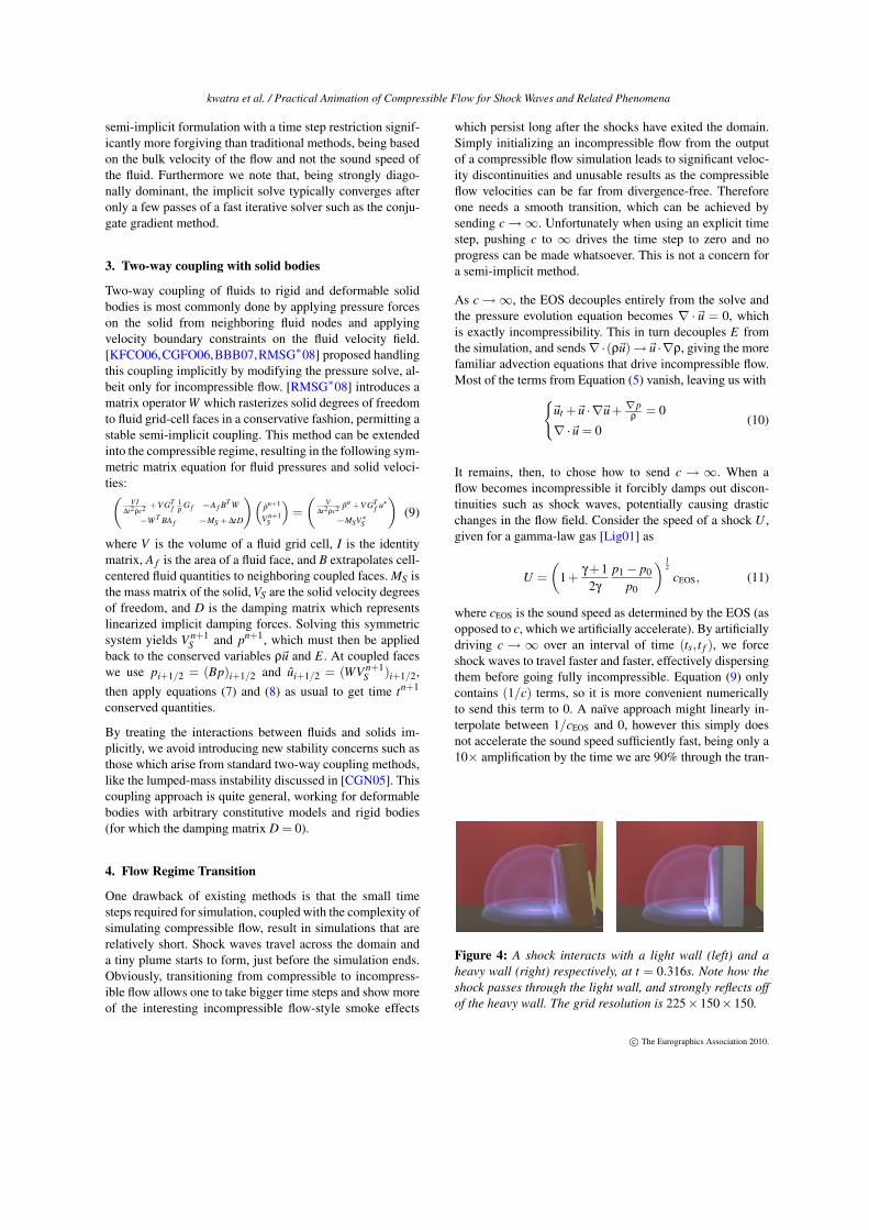
Figure 4: A shock interacts with a light wall (left) and aheavy wall (right) respectively, at t = 0.316s. Note how theshock passes through the light wall, and strongly reflects offof the heavy wall. The grid resolution is 225×150×150.



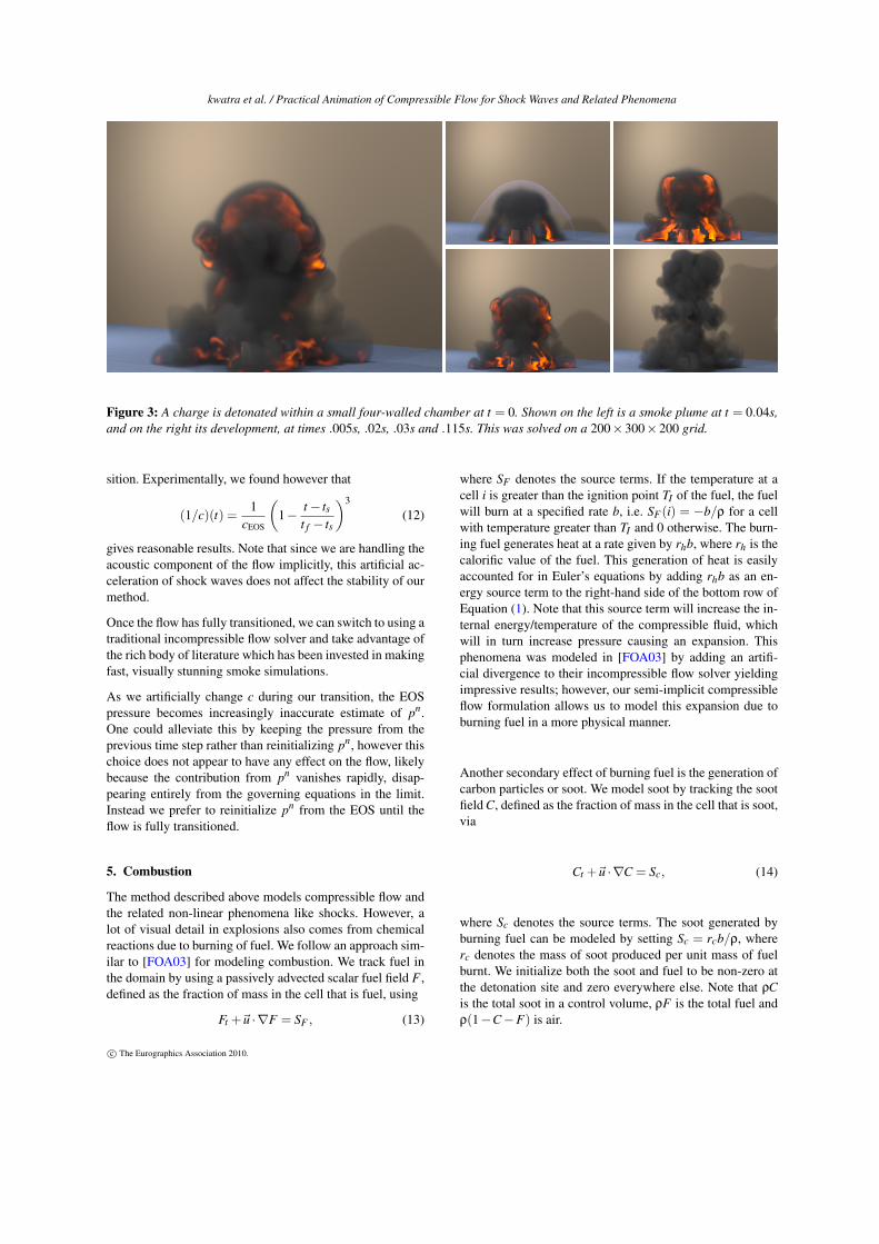
Figure 3: A charge is detonated within a small four-walled chamber at t = 0. Shown on the left is a smoke plume at t = 0.04s,and on the right its development, at times .005s, .02s, .03s and .115s. This was solved on a 200×300×200 grid.

sition. Experimentally, we found however that

(1/c)(t) =1

cEOS

(1− t− ts

t f − ts

)3

(12)

gives reasonable results. Note that since we are handling theacoustic component of the flow implicitly, this artificial ac-celeration of shock waves does not affect the stability of ourmethod.

Once the flow has fully transitioned, we can switch to using atraditional incompressible flow solver and take advantage ofthe rich body of literature which has been invested in makingfast, visually stunning smoke simulations.

As we artificially change c during our transition, the EOSpressure becomes increasingly inaccurate estimate of pn.One could alleviate this by keeping the pressure from theprevious time step rather than reinitializing pn, however thischoice does not appear to have any effect on the flow, likelybecause the contribution from pn vanishes rapidly, disap-pearing entirely from the governing equations in the limit.Instead we prefer to reinitialize pn from the EOS until theflow is fully transitioned.

5. Combustion

The method described above models compressible flow andthe related non-linear phenomena like shocks. However, alot of visual detail in explosions also comes from chemicalreactions due to burning of fuel. We follow an approach sim-ilar to [FOA03] for modeling combustion. We track fuel inthe domain by using a passively advected scalar fuel field F ,defined as the fraction of mass in the cell that is fuel, using

Ft +~u ·∇F = SF , (13)

where SF denotes the source terms. If the temperature at acell i is greater than the ignition point TI of the fuel, the fuelwill burn at a specified rate b, i.e. SF (i) = −b/ρ for a cellwith temperature greater than TI and 0 otherwise. The burn-ing fuel generates heat at a rate given by rhb, where rh is thecalorific value of the fuel. This generation of heat is easilyaccounted for in Euler’s equations by adding rhb as an en-ergy source term to the right-hand side of the bottom row ofEquation (1). Note that this source term will increase the in-ternal energy/temperature of the compressible fluid, whichwill in turn increase pressure causing an expansion. Thisphenomena was modeled in [FOA03] by adding an artifi-cial divergence to their incompressible flow solver yieldingimpressive results; however, our semi-implicit compressibleflow formulation allows us to model this expansion due toburning fuel in a more physical manner.

Another secondary effect of burning fuel is the generation ofcarbon particles or soot. We model soot by tracking the sootfield C, defined as the fraction of mass in the cell that is soot,via

Ct +~u ·∇C = Sc, (14)

where Sc denotes the source terms. The soot generated byburning fuel can be modeled by setting Sc = rcb/ρ, whererc denotes the mass of soot produced per unit mass of fuelburnt. We initialize both the soot and fuel to be non-zero atthe detonation site and zero everywhere else. Note that ρCis the total soot in a control volume, ρF is the total fuel andρ(1−C−F) is air.



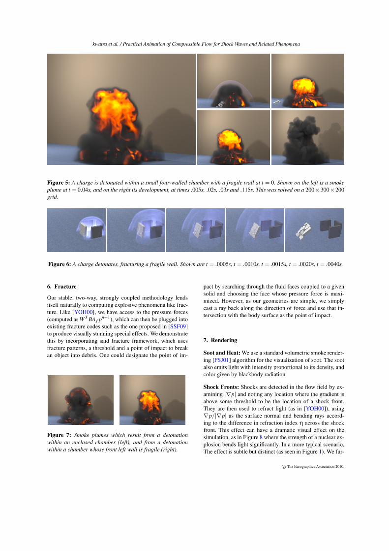
Figure 5: A charge is detonated within a small four-walled chamber with a fragile wall at t = 0. Shown on the left is a smokeplume at t = 0.04s, and on the right its development, at times .005s, .02s, .03s and .115s. This was solved on a 200×300×200grid.

Figure 6: A charge detonates, fracturing a fragile wall. Shown are t = .0005s, t = .0010s, t = .0015s, t = .0020s, t = .0040s.

6. Fracture

Our stable, two-way, strongly coupled methodology lendsitself naturally to computing explosive phenomena like frac-ture. Like [YOH00], we have access to the pressure forces(computed as W T BA f pn+1), which can then be plugged intoexisting fracture codes such as the one proposed in [SSF09]to produce visually stunning special effects. We demonstratethis by incorporating said fracture framework, which usesfracture patterns, a threshold and a point of impact to breakan object into debris. One could designate the point of im-

Figure 7: Smoke plumes which result from a detonationwithin an enclosed chamber (left), and from a detonationwithin a chamber whose front left wall is fragile (right).

pact by searching through the fluid faces coupled to a givensolid and choosing the face whose pressure force is maxi-mized. However, as our geometries are simple, we simplycast a ray back along the direction of force and use that in-tersection with the body surface as the point of impact.

7. Rendering

Soot and Heat: We use a standard volumetric smoke render-ing [FSJ01] algorithm for the visualization of soot. The sootalso emits light with intensity proportional to its density, andcolor given by blackbody radiation.

Shock Fronts: Shocks are detected in the flow field by ex-amining |∇p| and noting any location where the gradient isabove some threshold to be the location of a shock front.They are then used to refract light (as in [YOH00]), using∇p/|∇p| as the surface normal and bending rays accord-ing to the difference in refraction index η across the shockfront. This effect can have a dramatic visual effect on thesimulation, as in Figure 8 where the strength of a nuclear ex-plosion bends light significantly. In a more typical scenario,The effect is subtle but distinct (as seen in Figure 1). We fur-



ther enhance the visual impact of the shock by adding a blueemittance which scales with |∇p|, demonstrated in Figure 2.

8. Results

We simulate air as an ideal gas with γ = 1.4, with a rest statetemperature of Tatm = 290 K, zero initial velocity, and pres-sure of patm = 1.01325× 105 Pa, or atmospheric pressure.This gives a fluid of density ρ = 1.4 kg/m3, comparableto that of air. Unless otherwise noted we initialize a shockby instantaneously depositing a high internal energy intoan initial blast location, corresponding to a temperature of10×Tatm and pressure 103× patm. Boundary conditions areset to be atmospheric, permitting shocks to smoothly flowout of the domain.

All of our simulation are run with second order ENO [SO88]and third order Runge-Kutta. The examples took between 30minutes to several hours on our unoptimzied research codewith a lot of I/O. For the purposes of comparison we set upa simulation similar to Figure 11 in [SGTL09] and Figure 2in [YOH00]. The explicit version of our code ran in 4 min-utes and 24 seconds and the semi-implicit one in 3 minutes11 seconds, which is comparable to the numbers reportedin [SGTL09]. Even though the semi-implicit method wasfaster, if one only cares about the short time simulations withno rolling smoke, etc, explicit methods are just fine.

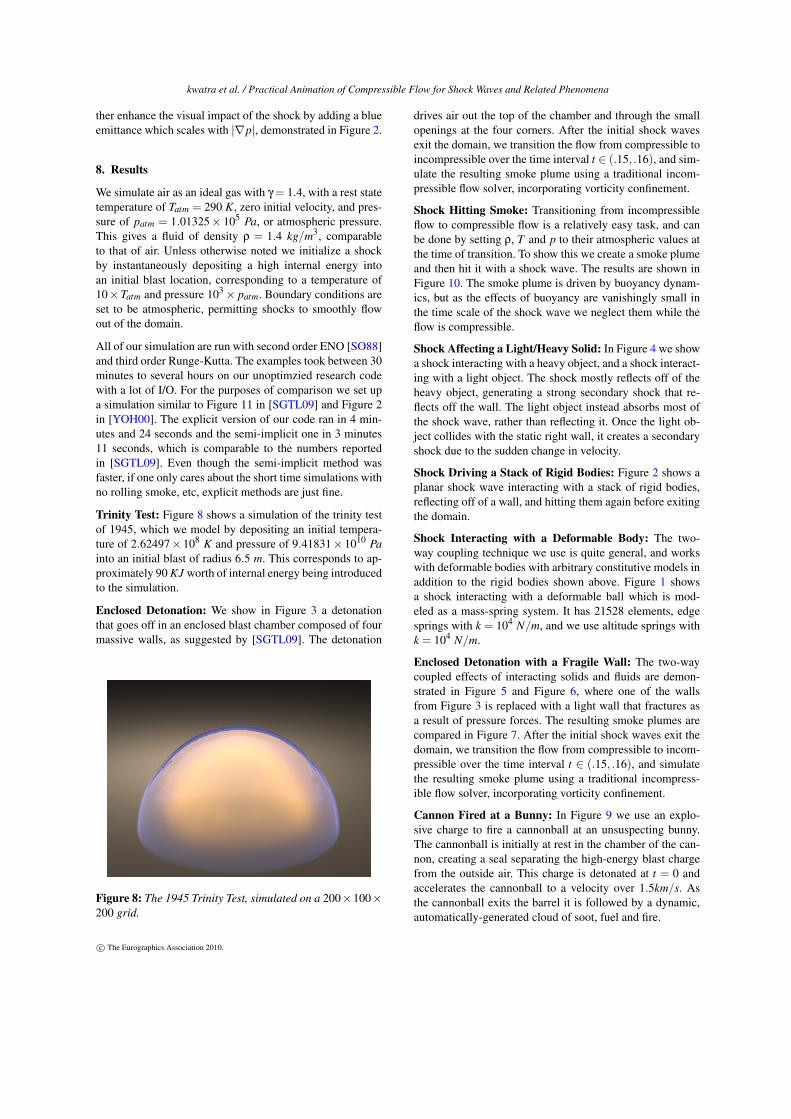
Trinity Test: Figure 8 shows a simulation of the trinity testof 1945, which we model by depositing an initial tempera-ture of 2.62497× 108 K and pressure of 9.41831× 1010 Painto an initial blast of radius 6.5 m. This corresponds to ap-proximately 90 KJ worth of internal energy being introducedto the simulation.

Enclosed Detonation: We show in Figure 3 a detonationthat goes off in an enclosed blast chamber composed of fourmassive walls, as suggested by [SGTL09]. The detonation

Figure 8: The 1945 Trinity Test, simulated on a 200×100×200 grid.

drives air out the top of the chamber and through the smallopenings at the four corners. After the initial shock wavesexit the domain, we transition the flow from compressible toincompressible over the time interval t ∈ (.15, .16), and sim-ulate the resulting smoke plume using a traditional incom-pressible flow solver, incorporating vorticity confinement.

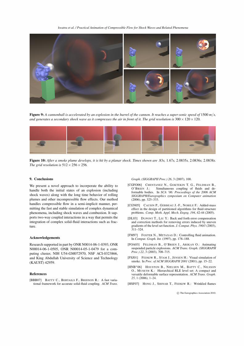
Shock Hitting Smoke: Transitioning from incompressibleflow to compressible flow is a relatively easy task, and canbe done by setting ρ, T and p to their atmospheric values atthe time of transition. To show this we create a smoke plumeand then hit it with a shock wave. The results are shown inFigure 10. The smoke plume is driven by buoyancy dynam-ics, but as the effects of buoyancy are vanishingly small inthe time scale of the shock wave we neglect them while theflow is compressible.

Shock Affecting a Light/Heavy Solid: In Figure 4 we showa shock interacting with a heavy object, and a shock interact-ing with a light object. The shock mostly reflects off of theheavy object, generating a strong secondary shock that re-flects off the wall. The light object instead absorbs most ofthe shock wave, rather than reflecting it. Once the light ob-ject collides with the static right wall, it creates a secondaryshock due to the sudden change in velocity.

Shock Driving a Stack of Rigid Bodies: Figure 2 shows aplanar shock wave interacting with a stack of rigid bodies,reflecting off of a wall, and hitting them again before exitingthe domain.

Shock Interacting with a Deformable Body: The two-way coupling technique we use is quite general, and workswith deformable bodies with arbitrary constitutive models inaddition to the rigid bodies shown above. Figure 1 showsa shock interacting with a deformable ball which is mod-eled as a mass-spring system. It has 21528 elements, edgesprings with k = 104 N/m, and we use altitude springs withk = 104 N/m.

Enclosed Detonation with a Fragile Wall: The two-waycoupled effects of interacting solids and fluids are demon-strated in Figure 5 and Figure 6, where one of the wallsfrom Figure 3 is replaced with a light wall that fractures asa result of pressure forces. The resulting smoke plumes arecompared in Figure 7. After the initial shock waves exit thedomain, we transition the flow from compressible to incom-pressible over the time interval t ∈ (.15, .16), and simulatethe resulting smoke plume using a traditional incompress-ible flow solver, incorporating vorticity confinement.

Cannon Fired at a Bunny: In Figure 9 we use an explo-sive charge to fire a cannonball at an unsuspecting bunny.The cannonball is initially at rest in the chamber of the can-non, creating a seal separating the high-energy blast chargefrom the outside air. This charge is detonated at t = 0 andaccelerates the cannonball to a velocity over 1.5km/s. Asthe cannonball exits the barrel it is followed by a dynamic,automatically-generated cloud of soot, fuel and fire.



Figure 9: A cannonball is accelerated by an explosion in the barrel of the cannon. It reaches a super-sonic speed of 1500 m/s,and generates a secondary shock wave as it compresses the air in front of it. The grid resolution is 300×120×120.

Figure 10: After a smoke plume develops, it is hit by a planar shock. Times shown are .83s, 1.67s, 2.0835s, 2.0836s, 2.0838s.The grid resolution is 512×256×256.

9. Conclusions

We present a novel approach to incorporate the ability tohandle both the initial states of an explosion (includingshock waves) along with the long time behavior of rollingplumes and other incompressible flow effects. Our methodhandles compressible flow in a semi-implicit manner, per-mitting the fast and stable simulation of complex dynamicalphenomena, including shock waves and combustion. It sup-ports two-way coupled interactions in a way that permits theintegration of complex solid-fluid interactions such as frac-ture.

Acknowledgements

Research supported in part by ONR N0014-06-1-0393, ONRN00014-06-1-0505, ONR N00014-05-1-0479 for a com-puting cluster, NIH U54-GM072970, NSF ACI-0323866,and King Abdullah University of Science and Technology(KAUST) 42959.

References[BBB07] BATTY C., BERTAILS F., BRIDSON R.: A fast varia-

tional framework for accurate solid-fluid coupling. ACM Trans.

Graph. (SIGGRAPH Proc.) 26, 3 (2007), 100.

[CGFO06] CHENTANEZ N., GOKTEKIN T. G., FELDMAN B.,O’BRIEN J.: Simultaneous coupling of fluids and de-formable bodies. In SCA ’06: Proceedings of the 2006 ACMSIGGRAPH/Eurographics symposium on Computer animation(2006), pp. 325–333.

[CGN05] CAUSIN P., GERBEAU J.-F., NOBILE F.: Added-masseffect in the design of partitioned algorithms for fluid-structureproblems. Comp. Meth. Appl. Mech. Engng. 194, 42-44 (2005).

[DL03] DUPONT T., LIU Y.: Back and forth error compensationand correction methods for removing errors induced by unevengradients of the level set function. J. Comput. Phys. 190/1 (2003),311–324.

[FM97] FOSTER N., METAXAS D.: Controlling fluid animation.In Comput. Graph. Int. (1997), pp. 178–188.

[FOA03] FELDMAN B., O’BRIEN J., ARIKAN O.: Animatingsuspended particle explosions. ACM Trans. Graph. (SIGGRAPHProc.) 22, 3 (2003), 708–715.

[FSJ01] FEDKIW R., STAM J., JENSEN H.: Visual simulation ofsmoke. In Proc. of ACM SIGGRAPH 2001 (2001), pp. 15–22.

[HNB∗06] HOUSTON B., NIELSEN M., BATTY C., NILSSONO., MUSETH K.: Hierarchical RLE level set: A compact andversatile deformable surface representation. ACM Trans. Graph.25, 1 (2006), 1–24.

[HSF07] HONG J., SHINAR T., FEDKIW R.: Wrinkled flames



and cellular patterns. ACM Transactions on Graphics (TOG) 26,3 (2007), 47.

[IJN09] IMAGIRE T., JOHAN H., NISHITA T.: A fast method forsimulating destruction and the generated dust and debris. TheVisual Computer 25, 5 (2009), 719–727.

[IKC04] IHM I., KANG B., CHA D.: Animation of reac-tive gaseous fluids through chemical kinetics. In Proc. of the2004 ACM SIGGRAPH/Eurographics Symp. on Comput. Anim.(2004), pp. 203–212.

[KFCO06] KLINGNER B. M., FELDMAN B. E., CHENTANEZN., O’BRIEN J. F.: Fluid animation with dynamic meshes. ACMTrans. Graph. 25, 3 (2006), 820–825.

[KJI07] KANG B., JANG Y., IHM I.: Animation of chemicallyreactive fluids using a hybrid simulation method. In Proceed-ings of the 2007 ACM SIGGRAPH/Eurographics symposium onComputer animation (2007), Eurographics Association, p. 208.

[KLLR05] KIM B.-M., LIU Y., LLAMAS I., ROSSIGNAC J.: Us-ing BFECC for fluid simulation. In Eurographics Workshop onNatural Phenomena 2005 (2005).

[KSGF09] KWATRA N., SU J., GRÉTARSSON J. T., FEDKIW R.:A method for avoiding the acoustic time step restriction in com-pressible flow. J. Comput. Phys. 228, 11 (2009), 4146–4161.

[LGF04] LOSASSO F., GIBOU F., FEDKIW R.: Simulating waterand smoke with an octree data structure. ACM Trans. Graph.(SIGGRAPH Proc.) 23 (2004), 457–462.

[Lig01] LIGHTHILL J.: Waves in fluids. Cambridge Univ Pr,2001.

[MMA99] MAZARAK O., MARTINS C., AMANATIDES J.: An-imating exploding objects. In Proc. of Graph. Interface 1999(1999), pp. 211–218.

[NF99] NEFF M., FIUME E.: A visual model for blast waves andfracture. In Proc. of Graph. Interface 1999 (1999), pp. 193–202.

[RMSG∗08] ROBINSON-MOSHER A., SHINAR T., GRÉTARS-SON J., SU J., FEDKIW R.: Two-way coupling of fluids to rigidand deformable solids and shells. ACM Transactions on Graph-ics 27, 3 (Aug. 2008), 46:1–46:9.

[RNGF03] RASMUSSEN N., NGUYEN D., GEIGER W., FEDKIWR.: Smoke simulation for large scale phenomena. ACM Trans.Graph. (SIGGRAPH Proc.) 22 (2003), 703–707.

[SFK∗08] SELLE A., FEDKIW R., KIM B., LIU Y., ROSSIGNACJ.: An unconditionally stable MacCormack method. Journal ofScientific Computing 35, 2 (2008), 350–371.

[SGTL09] SEWALL J., GALOPPO N., TSANKOV G., LIN M.: Vi-sual simulation of shockwaves. Graphical Models (2009).

[SMML07] SEWALL J., MECKLENBURG P., MITRAN S., LINM.: Fast fluid simulation using residual distribution schemes. InEurographics Workshop on Natural Phenomena (2007), pp. 47–54.

[SO88] SHU C.-W., OSHER S.: Efficient implementation of es-sentially non-oscillatory shock capturing schemes. J. Comput.Phys. 77 (1988), 439–471.

[SRF05] SELLE A., RASMUSSEN N., FEDKIW R.: A vortexparticle method for smoke, water and explosions. ACM Trans.Graph. (SIGGRAPH Proc.) 24, 3 (2005), 910–914.

[SSF09] SU J., SCHROEDER C., FEDKIW R.: Energy stabilityand fracture for frame rate rigid body simulations. In Proceedingsof the 2009 ACM SIGGRAPH/Eurographics Symp. on Comput.Anim. (2009), pp. 155–164.

[Sta99] STAM J.: Stable fluids. In Proc. of SIGGRAPH 99 (1999),pp. 121–128.

[SU94] STEINHOFF J., UNDERHILL D.: Modification of the Eu-ler equations for “vorticity confinement”: Application to the com-putation of interacting vortex rings. Phys. of Fluids 6, 8 (1994),2738–2744.

[TOT∗03] TAKESHITA D., OTA S., TAMURA M., FUJIMOTO T.,MURAOKA K., CHIBA N.: Particle-based visual simulation ofexplosive flames. In Computer Graphics and Applications, 2003.Proceedings. 11th Pacific Conference on (2003), pp. 482–486.

[YOH00] YNGVE G., O’BRIEN J., HODGINS J.: Animating ex-plosions. In Proc. SIGGRAPH 2000 (2000), vol. 19, pp. 29–36.



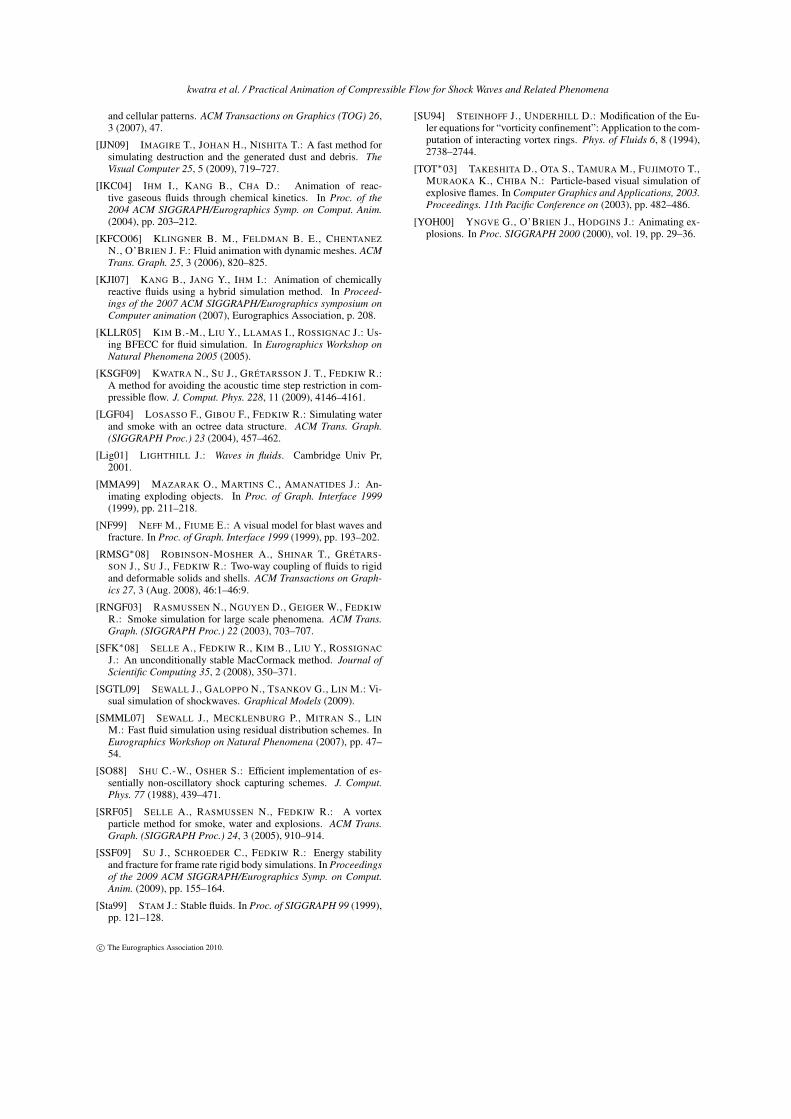
Figure 11: Compressible flow interacting with a variety of objects. (left) A bunny faces down a super-sonic cannonball, (middle)a detonation goes off in a four-walled chamber with a fragile wall, and (right) a shock tosses a stack of rigid bodies around.

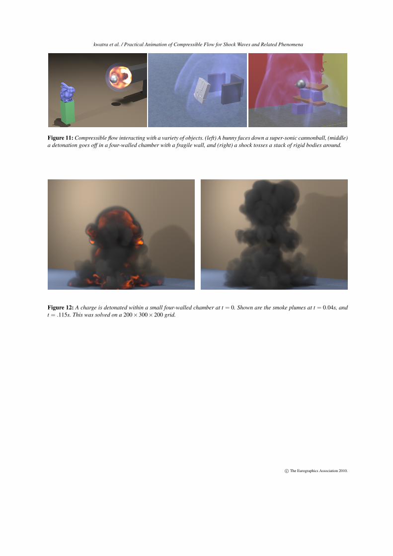
Figure 12: A charge is detonated within a small four-walled chamber at t = 0. Shown are the smoke plumes at t = 0.04s, andt = .115s. This was solved on a 200×300×200 grid.


Documents

Practical Animation of Compressible Flow for Shock - PhysBAM