Embed Size (px)
Citation preview

Power System Disturbance Analysis and Detection
Based on Wide-Area Measurements
Jingyuan Dong
Dissertation submitted to the faculty of the Virginia Polytechnic Institute and State
University in partial fulfillment of the requirements for the degree of
Doctor of Philosophy
In
Electrical Engineering
Committee Members:
Dr. James S. Thorp (Chair)
Dr. Yilu Liu
Dr. Virgilio A. Centeno
Dr. Pushkin Kachroo
Dr. Irene E. Leech
December 10, 2008
Blacksburg, Virginia
Keywords: Wide-Area Measurements, Frequency Monitoring Network, Power System
Dynamics, Power System Monitoring, Disturbance Detection.
© Copyright 2008, Jingyuan Dong
Power System Disturbance Analysis and Detection Based on Wide-Area
Measurements by
Jingyuan Dong
Abstract Wide-area measurement systems (WAMS) enable the monitoring of overall bulk
power systems and provide critical information for understanding and responding to
power system disturbances and cascading failures. The North American Frequency
Monitoring Network (FNET) takes GPS-synchronized wide-area measurements in a low-
cost, easily deployable manner at the 120 V distribution level, which presents more
opportunities to study power system dynamics. This work explores the topics of power
system disturbance analysis and detection by utilizing the wide-area measurements
obtained in the distribution networks.
In this work, statistical analysis is conducted based on the major disturbances in
the North American Interconnections detected by the FNET situation awareness system
between 2006 and 2008. Typical frequency patterns of the generation and load loss
events are analyzed for the three North American power Interconnections: the Eastern
Interconnection (EI), the Western Electricity Coordinating Council (WECC), and the
Electric Reliability Council of Texas (ERCOT). The linear relationship between
frequency deviation and frequency change rate during generation/loss mismatch events is
verified by the measurements in the three Interconnections. The relationship between the
generation/load mismatch and system frequency is also examined based on confirmed
generation loss events in the EI system. And a power mismatch estimator is developed to
improve the current disturbance detection program. Various types of power system
disturbances are examined based on frequency, voltage and phase angle to obtain the
event signatures in the measurements.
To better understand the propagation of disturbances in the power system, an
automated visualization tool is developed that can generate frequency and angle replays
of disturbances, as well as image snapshots. This visualization tool correlates the wide-
area measurements with geographical information by displaying the measurements over a

iii
geographical map. This work makes an attempt to investigate the visualization of the
angle profile in the wide-area power system to improve situation awareness.
This work explores the viability of relying primarily on distribution-level
measurements to detect and identify line outages, a topic not yet addressed in previous
works. Line outage sensitivity at different voltage levels in the Tennessee Valley
Authority (TVA) system is examined to analyze the visibility of disturbances from the
point of view of wide-area measurements. The sensor placement strategy is proposed for
better observability of the line trip disturbances. The characteristics of line outages are
studied extensively with simulations and real measurements. Line trip detection
algorithms are proposed that employs the information in frequency and phase angle
measurements. In spite of the limited FDR coverage and confirmed training cases, an
identification algorithm is developed which uses the information in the real
measurements as well as the simulation cases to determine the tripped line.

iv
Acknowledgments I would like to offer my first and foremost appreciation to Dr. James Thorp and
Dr. Yilu Liu for their patient guidance, support and encouragement, without which this
dissertation would not have been possible. I thank Dr. Liu for her support and
encouragement both in my academic and personal life. I can not be more grateful for her
invaluable counsel that has consistently inspired me to make research progress and
pursue personal improvement.
Thanks are extended to members in my advisory committee: Dr. Virgilio
Centeno, for providing encouragement and guidance in my academic progress and
teaching assistant assignments; Dr. Pushkin Kachroo and Dr. Irene Leech, for their
participation on my committee and valuable advices and comments.
Special thanks go to Dr. Richard Conners, for offering valuable suggestions to my
work. I would also like to thank Dr. Hengxu Zhang and Dr. Wei Li who had happily
shared with me their experiences and ideas concerning this work. I am thankful for the
foundational work and contributions especially from Dr. Jian Zuo, Dr. Kyung Soo Kook,
Dr. R. Matthew Gardner, Dr. Mark Baldwin, Kevin Khan, Lei Wang, Tao Xia, Jason
Bank, Yingchen Zhang, Dr. Jin Tao, Joshua K. Wang, and Jon Burgett.
Much appreciation goes to my colleagues in the power group: Dr. Dawei Fan, Dr.
Ming Zhou, Andrew Arana, Emanuel Bernabeu, Yishan Liang, for their support and
friendship.
Thanks to Lisa Beard and Gary Kobet of TVA for providing line outage data and
information, Tony Weekes of Manitoba Hydro for providing PMU measurements and
valuable insights, and Dave Bertagnolli of ISO New England for his industry insights.
Finally, I would like to express my deepest gratitude to my family: my father
Zhenxing Dong, my mother Qiutao Song and my brother Xiaolei Dong, for their endless
love and support. I thank my parents for being by my side while I am preparing this
dissertation. To me, their support is the most important thing in the world that encourages
me to fulfill my pursuit of a doctorate.
v
Table of Contents Abstract.............................................................................................................................. ii
Acknowledgments ............................................................................................................ iv
List of Figures................................................................................................................. viii
List of Tables ................................................................................................................ xviii
Chapter 1 Introduction............................................................................................... 1
1.1 Frequency Monitoring Network (FNET)............................................................ 1
1.2 Organization of Study ......................................................................................... 3
Chapter 2 Statistical Analysis of Disturbances in the North American
Interconnections................................................................................................................ 5
2.1 Statistical Analysis and Comparison of Major Disturbances in the Three
Interconnections.............................................................................................................. 6
2.2 Typical Frequency Excursions of the Disturbances.......................................... 13
2.3 Relationship between Frequency Change Rate and Total Frequency Variation
Amount ......................................................................................................................... 21
2.4 Power System Inertia and Frequency Response Characteristic........................ 24
2.5 Frequency Restoration Characteristics ............................................................. 34
Chapter 3 Analysis of Major Disturbances in the Eastern Interconnection ....... 37
3.1 Three-phase Fault.............................................................................................. 37
3.2 Multi-disturbance Event.................................................................................... 41
3.3 Islanding............................................................................................................ 44
3.3.1 Recordings from FDRs ............................................................................. 45
3.3.2 Comparisons of Measurements from FDR and PMU............................... 50
3.4 Florida Outage .................................................................................................. 53
3.5 Faults in HVDC Systems .................................................................................. 57
3.5.1 Events in the Quebec – New England HVDC Interconnection on June 20
and October 25, 2008................................................................................................ 58
3.5.2 Event in the Nelson River HVDC System on June 2, 2008...................... 62
3.6 Dynamic Performance of AD/DC Systems ...................................................... 68
Chapter 4 Visualization of Wide-Area Measurements.......................................... 74
4.1 Motivation Example.......................................................................................... 74
vi
4.2 Visualization Tool Overview............................................................................ 77
4.2.1 The Visualization Toolkit ......................................................................... 77
4.2.2 MATCOM Math Library .......................................................................... 78
4.3 Design of the Visualization Tool ...................................................................... 78
4.3.1 Read Measurements .................................................................................. 80
4.3.2 Generate Measurement Matrices for Display ........................................... 83
4.3.3 Form Animation Frames ........................................................................... 84
4.4 Application Examples....................................................................................... 86
4.4.1 Angle Replay for the Florida Outage........................................................ 86
4.4.2 Angle Distribution from PSS/E ................................................................ 90
4.4.3 Angle Distribution from Real Measurements ........................................... 92
4.4.4 Visualization with Google Earth............................................................... 95
Chapter 5 Line Trip Detection................................................................................. 97
5.1 Line Trip Sensitivity Study............................................................................... 97
5.2 FDR Placement Strategy................................................................................. 111
5.3 Line Trip Detection with Frequency............................................................... 113
5.4 Line Trip Detection with Angle...................................................................... 117
5.4.1 Comparisons between Triggering Signals .............................................. 118
5.4.2 Line Trip Trigger Based on De-trended Angle....................................... 122
5.4.3 Line Trip Trigger Based on Relative Angle ........................................... 125
5.5 Summary ......................................................................................................... 127
Chapter 6 Line Trip Identification........................................................................ 129
6.1 Line Trip Characteristics – A Close Examination .......................................... 129
6.1.1 Line Trip Signatures in PSS/E Simulation.............................................. 129
6.1.2 Line Trip Signatures in Real Measurements........................................... 136
6.2 500 kV and 161 kV Line Trip Detection ........................................................ 138
6.2.1 500 kV Line Trip Detection Simulation Study ....................................... 138
6.2.2 161 kV Line Trip Detection Simulation Study ....................................... 142
6.3 Line Trip Identification................................................................................... 150
6.3.1 Line Trip Identification Algorithm ......................................................... 151
6.3.2 Testing Examples.................................................................................... 156
vii
6.3.3 Discussion............................................................................................... 163
Chapter 7 Conclusions and Future Work............................................................. 167
7.1 Conclusions..................................................................................................... 167
7.2 Contributions................................................................................................... 169
7.3 Potential Future Work..................................................................................... 170
References...................................................................................................................... 173
Appendix I. Confirmed Disturbances in the EI from 2007 to 2008.......................... 180
Appendix II. Development Manual for the Visualization Tool ................................ 185
1. Install the Visualization Toolkit (VTK).............................................................. 185
2. Install and Configure MATCOM Math Library ................................................. 187
3. Create a C++ Project........................................................................................... 189
4. The Structure of the Program.............................................................................. 191
Appendix III. KML File for Overlaying an Image on Google Earth....................... 202

viii
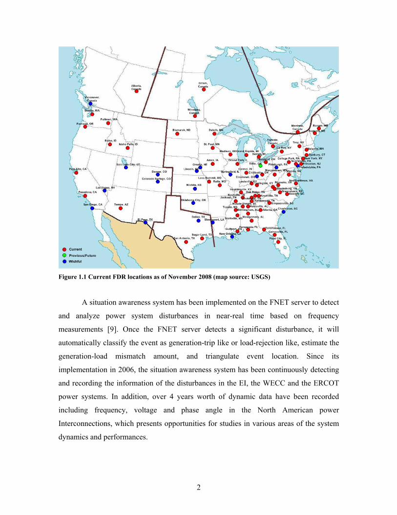
List of Figures Figure 1.1 Current FDR locations as of November 2008 (map source: USGS)................. 2
Figure 2.1 Major frequency disturbances (estimated generation-load mismatch > 500MW)
in the EI for each month...................................................................................................... 7
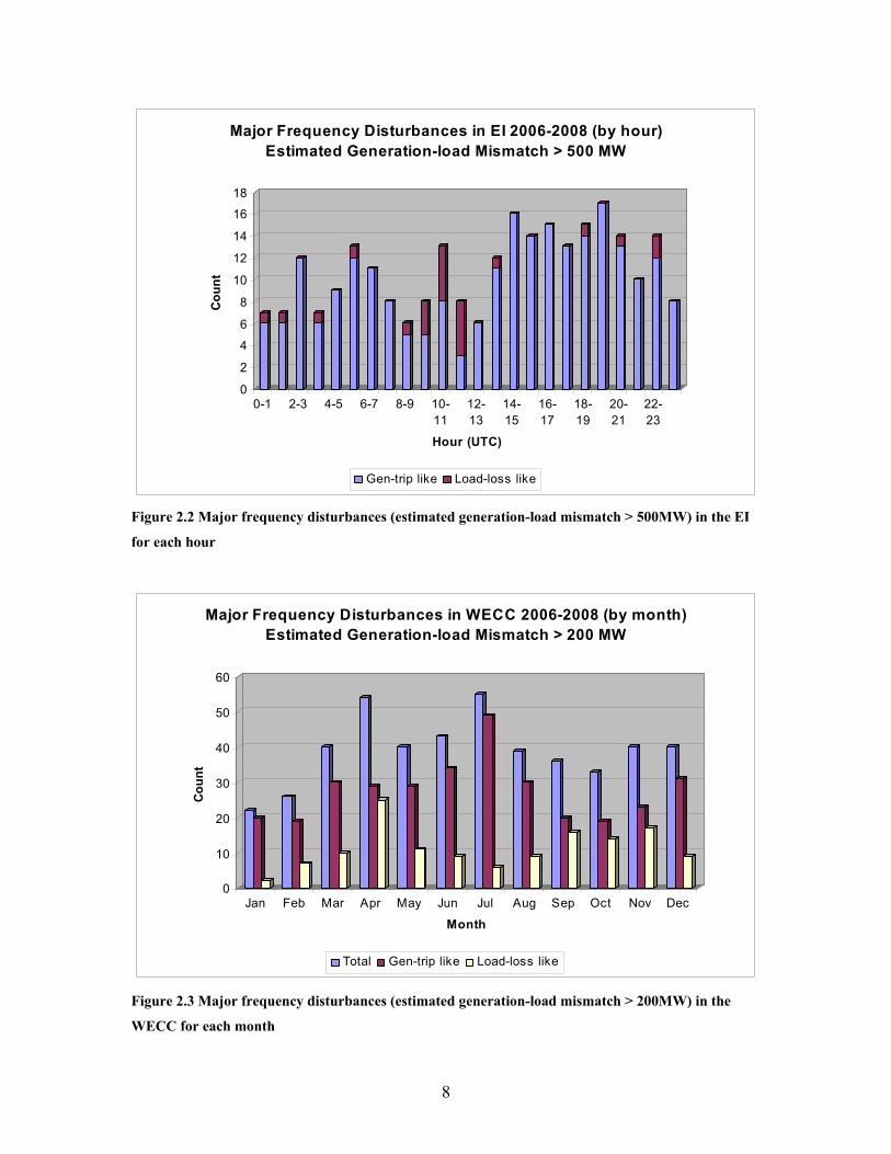
Figure 2.2 Major frequency disturbances (estimated generation-load mismatch > 500MW)
in the EI for each hour ........................................................................................................ 8
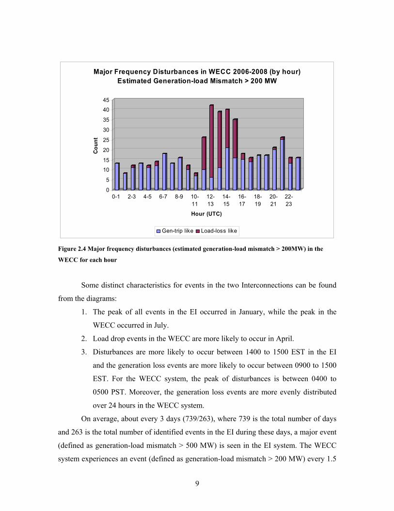
Figure 2.3 Major frequency disturbances (estimated generation-load mismatch > 200MW)
in the WECC for each month.............................................................................................. 8
Figure 2.4 Major frequency disturbances (estimated generation-load mismatch > 200MW)
in the WECC for each hour................................................................................................. 9
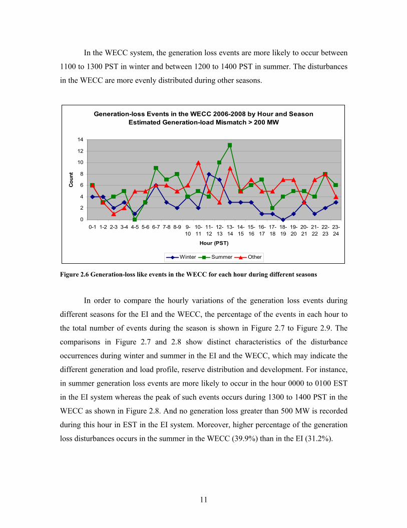
Figure 2.5 Generation-loss like events in the EI for each hour during different seasons . 10
Figure 2.6 Generation-loss like events in the WECC for each hour during different
seasons .............................................................................................................................. 11
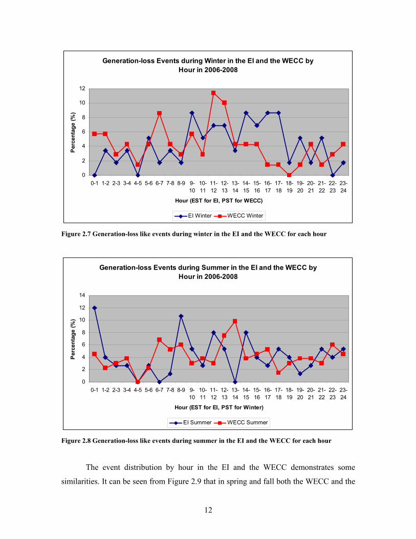
Figure 2.7 Generation-loss like events during winter in the EI and the WECC for each
hour ................................................................................................................................... 12
Figure 2.8 Generation-loss like events during summer in the EI and the WECC for each
hour ................................................................................................................................... 12
Figure 2.9 Generation-loss like events during other months in the EI and the WECC for
each hour........................................................................................................................... 13
Figure 2.10 Frequency excursion of a generator trip in the EI ......................................... 14
Figure 2.11 Detail of the initial frequency drop of the generator trip event in Figure 2.10
........................................................................................................................................... 14
Figure 2.12 Typical generation-loss like events in the EI system .................................... 15
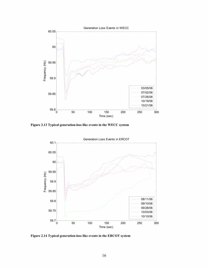
Figure 2.13 Typical generation-loss like events in the WECC system............................. 16
Figure 2.14 Typical generation-loss like events in the ERCOT system........................... 16
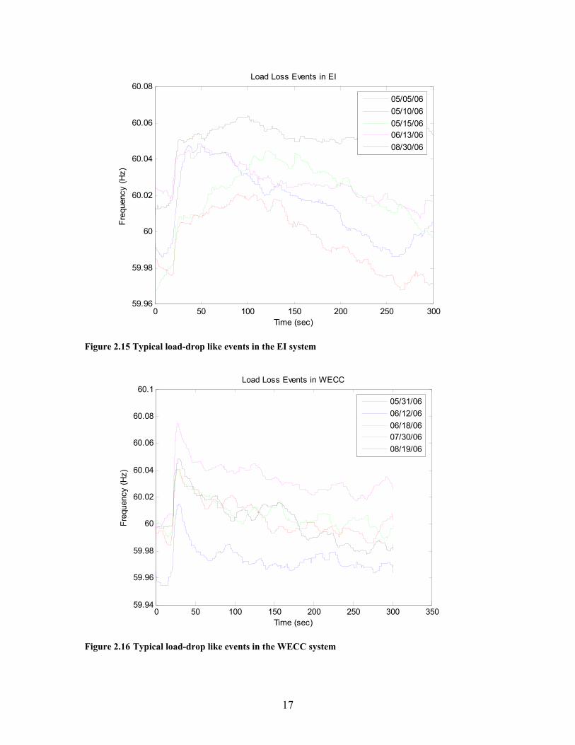
Figure 2.15 Typical load-drop like events in the EI system ............................................. 17
Figure 2.16 Typical load-drop like events in the WECC system ..................................... 17
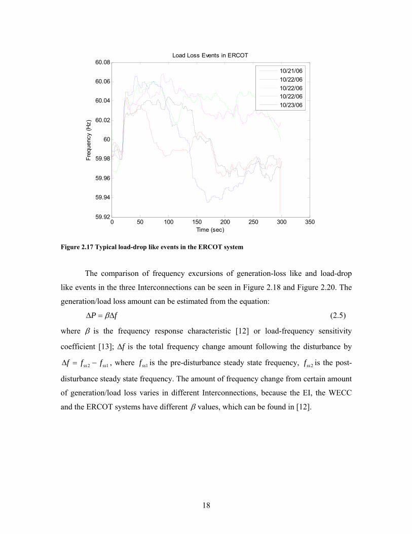
Figure 2.17 Typical load-drop like events in the ERCOT system.................................... 18
Figure 2.18 Generation-loss like events in the three Interconnections............................. 19
ix
Figure 2.19 Detail of the initial frequency drop for generation-loss like events in the three
Interconnections................................................................................................................ 19
Figure 2.20 Load-drop like events in the three Interconnections ..................................... 20
Figure 2.21 An example synchronous power system with m machines and p loads........ 22
Figure 2.22 Equivalent one-machine system of the example multiple machine system .. 23
Figure 2.23 Relationship between maximum frequency change rate and total amount of
frequency deviation........................................................................................................... 24
Figure 2.24 Generation/load mismatch vs. frequency change rate for generator trip events
in the EI from 2007 to 2008.............................................................................................. 25
Figure 2.25 Generation/Load mismatch vs. frequency change rate for summer generator
trips ................................................................................................................................... 27
Figure 2.26 Generation/Load mismatch vs. frequency change rate for winter generator
trips ................................................................................................................................... 27
Figure 2.27 Generation/Load mismatch vs. frequency change rate for spring and fall
generator trips ................................................................................................................... 28
Figure 2.28 Generation/Load mismatch vs. frequency change rate for generator trips
larger than 1000 MW........................................................................................................ 28
Figure 2.29 Generation/Load mismatch vs. frequency change rate for generator trips
smaller than 1000 MW...................................................................................................... 29
Figure 2.30 Generation/load mismatch vs. frequency deviation for generator trip events in
the EI from 2007 to 2008.................................................................................................. 30
Figure 2.31 Generation/load mismatch vs. frequency deviation for summer generator trips
........................................................................................................................................... 31
Figure 2.32 Generation/load mismatch vs. frequency deviation for winter generator trips
........................................................................................................................................... 31
Figure 2.33 Generation/load mismatch vs. frequency deviation for spring and fall
generator trips ................................................................................................................... 32
Figure 2.34 Generation/Load mismatch vs. frequency deviation for generator trips larger
than 1000 MW .................................................................................................................. 32
Figure 2.35 Generation/Load mismatch vs. frequency deviation for generator trips
smaller than 1000 MW...................................................................................................... 33
x
Figure 2.36 Generation/load mismatch estimator............................................................. 34
Figure 3.1 Frequency excursion during the three-phase disturbance ............................... 38
Figure 3.2 Frequency detail of the three-phase disturbance ............................................. 39
Figure 3.3 Phase angle during the three-phase disturbance.............................................. 40
Figure 3.4 Voltage dip caused by the three-phase disturbance......................................... 40
Figure 3.5 Frequency excursion during the multi-disturbance event ............................... 42
Figure 3.6 Frequency detail of line events before the generation trip .............................. 42
Figure 3.7 Frequency detail of the generation trip during the multi-disturbance event ... 43
Figure 3.8 Phase angle during the multi-disturbance event.............................................. 43
Figure 3.9 Voltage magnitude during the multi-disturbance event .................................. 44
Figure 3.10 Frequency excursion during the islanding event. Note 3 FDRs in this plot
show frequency excursions close to 61 Hz in the islanded system................................... 46
Figure 3.11 Frequency detail of line trip events before the islanding started................... 46
Figure 3.12 Frequency detail showing the start of the islanding - the remainder of the
interconnection.................................................................................................................. 47
Figure 3.13 Frequency detail showing the start of the islanding - island ......................... 47
Figure 3.14 Phase angle of the islanding event. 3 FDRs (40, 41 and 43) provided the
angle data in the runaway system as indicated by the angle acceleration top part while the
rest are in the main system................................................................................................ 49
Figure 3.15 Voltage magnitude of the islanding event ..................................................... 49
Figure 3.16 Voltage detail showing the start of the islanding event................................. 50
Figure 3.17 Frequency comparison of PMU and FDR both in the islanded area............. 51
Figure 3.18 Phase angle comparison of PMU and FDR showing the islanding event. Note
that the 3 FDR plots are on top of each other shown as one lower curve......................... 51
Figure 3.19 Voltage magnitude comparison of PMU and FDR both in the islanded area 52
Figure 3.20 Voltage magnitude comparison detail of PMU and FDR both in the islanded
area.................................................................................................................................... 52
Figure 3.21 Frequency excursion between 18:00 to 19:00 UTC for the Florida outage .. 54
Figure 3.22 Frequency excursion over a three-minute time window for the Florida outage
........................................................................................................................................... 55
Figure 3.23 Detail of frequency oscillations during the Florida outage ........................... 55
xi
Figure 3.24 Normalized voltage showing the voltage depression during the Florida outage
........................................................................................................................................... 56
Figure 3.25 Detail of angle oscillations during the Florida outage (referred to FDR4) ... 56
Figure 3.26 Configuration of bipolar HVDC link ............................................................ 57
Figure 3.27 Location of the Quebec – New England Phase II HVDC transmission line
(map source: USGS) ......................................................................................................... 58
Figure 3.28 Frequency of the Quebec – New England HVDC event on June 20, 2008... 59
Figure 3.29 Relative Angle of the Quebec – New England HVDC event on June 20, 2008
(FDR 569 as reference)..................................................................................................... 60
Figure 3.30 Frequency of the Quebec – New England HVDC event on October 25, 2008
........................................................................................................................................... 61
Figure 3.31 Angle of the Quebec – New England HVDC event on October 25, 2008
(FDR 569 as reference)..................................................................................................... 61
Figure 3.32 Location of the Nelson River HVDC transmission system (map source:
NERC)............................................................................................................................... 62
Figure 3.33 20-minute frequency excursion of the Nelson River HVDC system event at
both sides of the HVDC lines ........................................................................................... 63
Figure 3.34 20-minute frequency excursion of the Nelson River HVDC system event at
the Dorsey side.................................................................................................................. 64
Figure 3.35 Frequency detail of the Nelson River HVDC system event at Radisson (1). 65
Figure 3.36 Frequency detail of the Nelson River HVDC system event at Winnipeg (1) 66
Figure 3.37 Frequency detail of the Nelson River HVDC system event at Radisson (2). 66
Figure 3.38 Frequency detail of the Nelson River HVDC system event at Winnipeg (2) 67
Figure 3.39 Relative Angle of the Nelson River HVDC system event at the Dorsey side
(FDR569 as reference)...................................................................................................... 67
Figure 3.40 Frequency observed at both sides of the HVDC line during a generation loss
event in the EI on June 24, 2008....................................................................................... 69
Figure 3.41 Frequency observed at both sides of the HVDC line during a load loss event
in the EI on November 2, 2008......................................................................................... 70
Figure 3.42 Frequency observed at both sides of the HVDC line during a load loss event
in the EI on May 19, 2008 ................................................................................................ 70
xii
Figure 3.43 Frequency in the EI and Quebec during a generator trip event in the EI ...... 72
Figure 3.44 Frequency in the EI and the WECC during a load loss event in the EI ........ 72
Figure 3.45 Frequency in the EI and the ERCOT during a generator trip event in the EI 73
Figure 4.1 Frequency oscillations measured by all available FDRs in the EI during the
Florida outage on February 26, 2008................................................................................ 74
Figure 4.2 Snapshot of the frequency replay of the Florida outage (1) ............................ 75
Figure 4.3 Snapshot of the frequency replay of the Florida outage (2) ............................ 75
Figure 4.4 Snapshot of the frequency replay of the Florida outage (3) ............................ 76
Figure 4.5 Snapshot of the frequency replay of the Florida outage (4) ............................ 76
Figure 4.6 Flowchart of the automated replay tool........................................................... 79
Figure 4.7 Procedures to read data.................................................................................... 80
Figure 4.8 An example of UnitConfig.txt......................................................................... 81
Figure 4.9 Illustration of managing the FDR information with the vector structure........ 81
Figure 4.10 An example of EventLocation.txt.................................................................. 82
Figure 4.11 An example of the event data file.................................................................. 83
Figure 4.12 Procedures to generate measurement matrices for display............................ 84
Figure 4.13 The pipeline execution model in VTK .......................................................... 84
Figure 4.14 Dataset types in VTK .................................................................................... 85
Figure 4.15 Procedures to form animation frames............................................................ 86
Figure 4.16 Pre-processed angle of the Florida outage (FDR4 as reference)................... 87
Figure 4.17 Snapshot of the angle replay of the Florida outage (1) ................................. 88
Figure 4.18 Snapshot of the angle replay of the Florida outage (2) ................................. 88
Figure 4.19 Snapshot of the angle replay of the Florida outage (3) ................................. 89
Figure 4.20 Snapshot of the angle replay of the Florida outage (4) ................................. 89
Figure 4.21 Angle distribution in the EI from PSS/E simulation with 57 buses monitored
........................................................................................................................................... 90
Figure 4.22 Steady-state angles in the EI from PSS/E simulation on polar plane............ 91
Figure 4.23 Angle distribution in the EI from PSS/E simulation with 154 buses monitored
........................................................................................................................................... 91
Figure 4.24 Angle distribution in the EI from real measurements at 06:00 UTC on August
16, 2008............................................................................................................................. 92
xiii
Figure 4.25 Angles in the EI on polar plane at 06:00 UTC on August 16, 2008.............. 93
Figure 4.26 Angles in the EI on polar plane after adjusting phase shifts ......................... 93
Figure 4.27 Angle distribution in the EI from real measurements after adjusting phase
shifts.................................................................................................................................. 94
Figure 4.28 Frequency replay image overlaid on Google Earth (http://earth.google.com/)
........................................................................................................................................... 96
Figure 5.1 Locations of selected transmission lines in the TVA system for line trip
sensitivity study (map source: TVA) ................................................................................ 98
Figure 5.2 Frequency of the 500 kV Roane – Watts Bar line trip from PSS/E simulation
........................................................................................................................................... 99
Figure 5.3 Angle of the 500 kV Roane – Watts Bar line trip from PSS/E simulation ... 100
Figure 5.4 Frequency sensitivity map for the 500 kV Roane – Watts Bar line trip (map
source: TVA) .................................................................................................................. 101
Figure 5.5 Angle sensitivity map for the 500 kV Roane – Watts Bar line trip (map source:
TVA) ............................................................................................................................... 101
Figure 5.6 Frequency of the 161 kV Volunteer – Knoxville line trip from PSS/E
simulation........................................................................................................................ 102
Figure 5.7 Angle of the 161 kV Volunteer – Knoxville line trip from PSS/E simulation
......................................................................................................................................... 103
Figure 5.8 Frequency sensitivity map for the 161 kV Volunteer – Knoxville line trip (map
source: TVA) .................................................................................................................. 103
Figure 5.9 Angle sensitivity map for the 161 kV Volunteer – Knoxville line trip (map
source: TVA) .................................................................................................................. 104
Figure 5.10 Frequency of the 69 kV Melton Hill – Farragut line trip from PSS/E
simulation........................................................................................................................ 104
Figure 5.11 Angle of the 69 kV Melton Hill – Farragut line trip from PSS/E simulation
......................................................................................................................................... 105
Figure 5.12 Frequency sensitivity map for the 69 kV Melton Hill – Farragut line trip
(map source: TVA) ......................................................................................................... 105
Figure 5.13 Angle sensitivity map for the 69 kV Melton Hill – Farragut line trip (map
source: TVA) .................................................................................................................. 106
xiv
Figure 5.14 Frequency of the 230 kV Widows Creek – Crawfish line trip from PSS/E
simulation........................................................................................................................ 107
Figure 5.15 Angle of the 230 kV Widows Creek – Crawfish line trip from PSS/E
simulation........................................................................................................................ 107
Figure 5.16 Frequency sensitivity map for the 230 kV Widows Creek – Crawfish line trip
(map source: TVA) ......................................................................................................... 108
Figure 5.17 Angle sensitivity map for the 230 kV Widows Creek – Crawfish line trip
(map source: TVA) ......................................................................................................... 108
Figure 5.18 Frequency of the 230 kV West Ringgold – Alpha line trip from PSS/E
simulation........................................................................................................................ 109
Figure 5.19 Angle of the 230 kV West Ringgold – Alpha line trip from PSS/E simulation
......................................................................................................................................... 110
Figure 5.20 Frequency sensitivity map for the 230 kV West Ringgold – Alpha line trip
(map source: TVA) ......................................................................................................... 110
Figure 5.21 Angle sensitivity map for the 230 kV West Ringgold – Alpha line trip (map
source: TVA) .................................................................................................................. 111
Figure 5.22 Proposed FDR locations (map source: TVA).............................................. 113
Figure 5.23 Frequency of a line trip event...................................................................... 114
Figure 5.24 Line trip trigger using frequency................................................................. 114
Figure 5.25 Example raw frequency............................................................................... 115
Figure 5.26 Frequency after the median filter ................................................................ 115
Figure 5.27 De-trended frequency data .......................................................................... 116
Figure 5.28 Relative Phase angle (VT as reference) of the line trip on March 28, 2007 118
Figure 5.29 De-trended angle of the line trip on March 28, 2007 .................................. 119
Figure 5.30 Unwrapped angle of the line trip on March 28, 2007.................................. 119
Figure 5.31 Relative angle of the line trip on April 11, 2007 (VT as reference)............ 120
Figure 5.32 De-trended angle of the line trip on April 11, 2007 .................................... 121
Figure 5.33 Unwrapped angle of the line trip on April 11, 2007.................................... 121
Figure 5.34 Line trip trigger using de-trended phase angle ............................................ 122
Figure 5.35 Example raw angle data............................................................................... 123
Figure 5.36 Unwrapped angle data ................................................................................. 123
xv
Figure 5.37 All angle data are scaled to start from zero. ................................................ 124
Figure 5.38 De-trended angle data.................................................................................. 124
Figure 5.39 De-trended data after removing the noises.................................................. 125
Figure 5.40 Flowchart of the line trip trigger based on relative angle............................ 126
Figure 5.41 Relative angle for a line trip event (FDR35 as reference)........................... 127
Figure 6.1 Frequency from tripping the 500 kV Cumberland – Johnsonville line after a
line fault .......................................................................................................................... 130
Figure 6.2 Phase angle from tripping the 500 kV Cumberland – Johnsonville line after a
line fault .......................................................................................................................... 131
Figure 6.3 Frequency from tripping the 500 kV Cumberland – Johnsonville line without
fault ................................................................................................................................. 132
Figure 6.4 Phase angle from tripping the 500 kV Cumberland – Johnsonville line without
fault ................................................................................................................................. 132
Figure 6.5 Frequency and angle derivative from PSS/E on tripping 500 kV Cumberland –
Johnsonville line ............................................................................................................. 134
Figure 6.6 Integrated frequency from PSS/E on tripping 500 kV Cumberland –
Johnsonville line ............................................................................................................. 135
Figure 6.7 Phase angle and integrated frequency plus initial angle state change from
PSS/E on tripping 500 kV Cumberland – Johnsonville line........................................... 135
Figure 6.8 Frequency measurements for the line trip at the 500 kV Cumberland –
Johnsonville line ............................................................................................................. 137
Figure 6.9 Relative angle for the line trip at the 500 kV Cumberland – Johnsonville line
(FDR4 as reference)........................................................................................................ 137
Figure 6.10 Frequency form PSS/E on tripping the 500 kV Paradise – Montgomery line
......................................................................................................................................... 140
Figure 6.11 Phase angle form PSS/E on tripping the 500 kV Paradise – Montgomery line
......................................................................................................................................... 140
Figure 6.12 Frequency form PSS/E on tripping the 500 kV Raccoon Mountain – Widows
Creek line ........................................................................................................................ 141
Figure 6.13 Phase angle form PSS/E on tripping the 500 kV Raccoon Mountain –
Widows Creek line.......................................................................................................... 142
xvi
Figure 6.14 161 kV line loading conditions in the TVA system in PSS/E..................... 144
Figure 6.15 Partial one-line diagram of the EI system showing the tripping of the 161 kV
Widows Creek – Oglethr line (The red arrow indicates the direction of the power flow on
the line.) .......................................................................................................................... 147
Figure 6.16 Magnified frequency after tripping the 161 kV Widows Creek – Oglethr line
......................................................................................................................................... 148
Figure 6.17 Magnified angle after tripping the 161 kV Widows Creek – Oglethr line.. 148
Figure 6.18 An example showing the frequency delay of arrival................................... 150
Figure 6.19 The estimated disturbance location of the example. (The estimated location is
shown as the red circle. The real location is shown as the blue dot. Map source: USGS)
......................................................................................................................................... 151
Figure 6.20 Flowchart of building the line trip case library from simulation data......... 152
Figure 6.21 Line trip identification procedures .............................................................. 153
Figure 6.22 Angle peak detection from the relative angle.............................................. 154
Figure 6.23 The area around the Cumberland – Johnsonville line (marked with the red
cross. map source: TVA) ................................................................................................ 156
Figure 6.24 Angle from PSS/E on tripping the 500 kV Cumberland – Johnsonville line
with noises added (SNR: 20 dB)..................................................................................... 157
Figure 6.25 Line trip locations (marked as red crosses) and current FDR locations around
the TVA area (marked as red dots. map source: TVA) .................................................. 159
Figure 6.26 Angle discontinuity problem due to old firmware ...................................... 160
Figure 6.27 Relative angle of the Sequoyah – Bradley line trip on June 28, 2007 (FDR4
as reference) .................................................................................................................... 161
Figure 6.28 Relative angle of the Cumberland – Davidson line trip on December 16, 2006
(FDR4 as reference)........................................................................................................ 162
Figure 6.29 Frequency of the line trip at Browns Ferry – Union on November 13, 2007
......................................................................................................................................... 164
Figure 6.30 Frequency of the line trip at Browns Ferry – Union on April 10, 2008 ...... 164
Figure 6.31 Relative angle of the line trip at Browns Ferry – Union on November 13,
2007 (FDR4 as reference)............................................................................................... 165
xvii
Figure 6.32 Relative angle of the line trip at Browns Ferry – Union on April 10, 2008
(FDR4 as reference)........................................................................................................ 165
Figure II. 1 Run Cmake to build the VTK libraries........................................................ 186
Figure II. 2 Build the VTK libraries in MSVC++ .......................................................... 187
Figure II. 3 Install MATCOM math library.................................................................... 188
Figure II. 4 Test the installation of MATCOM............................................................... 189
Figure II. 5 Procedures to read data ................................................................................ 192
Figure II. 6 Example of UnitConfig.txt .......................................................................... 193
Figure II. 7 Illustration of the vector of the FDR information........................................ 193
Figure II. 8 Example of EventLocation.txt ..................................................................... 194
Figure II. 9 Procedure of data conditioning .................................................................... 195
Figure II. 10 Example of YYYYMMDD-HHMMSS-XXXX.txt file ............................ 195
Figure II. 11 Format of the UnitData vector ................................................................... 196
Figure II. 12 Procedures to generate measurement matrix ............................................. 198
Figure II. 13 Procedures to generate a movie frame....................................................... 201
xviii
List of Tables Table 2.1 Estimation of the inertia in the EI..................................................................... 26
Table 2.2 Estimation of the frequency response characteristic in the EI.......................... 30
Table 2.3 Statistics of frequency restoration characteristic of generation-loss like events
in the three Interconnections from Jan. to Oct. 2006........................................................ 36
Table 2.4 Statistics of frequency restoration characteristic of some generation trips in the
EI control areas ................................................................................................................. 36
Table 5.1 Selected transmission lines for the sensitivity study ........................................ 98
Table 5.2 500 kV line outage occurrences in TVA from January 2007 to June 2008.... 112
Table 5.3 Test results of the line trip trigger using frequency data ................................ 117
Table 6.1 Summary of simulation on 500 kV line trips in the TVA system .................. 139
Table 6.2 Summary of the voltage levels in the TVA transmission system identified in
PSS/E .............................................................................................................................. 143
Table 6.3 Summary of simulation results of the 161 kV line trips ................................. 145
Table 6.4 The power flow range and observable 161 kV line trips in the PSS/E simulation
......................................................................................................................................... 145
Table 6.5 Selected 161 kV line trip cases for the estimation of required FDR number . 146
Table 6.6 Estimation of the FDRs required to detect the 161 kV line trips in the TVA
system (N: not observable) ............................................................................................. 149
Table 6.7 Test results on the simulation data for the Cumberland – Johnsonville line trip
......................................................................................................................................... 157
Table 6.8 Test results on the simulation data for the Cumberland – Johnsonville line trip
with noises added (SNR: 20 dB)..................................................................................... 158
Table 6.9 Test results on the simulation data for the Cumberland – Johnsonville line trip
with noises added (SNR: 15 dB)..................................................................................... 158
Table 6.10 Test results on the simulation data for the Cumberland – Johnsonville line trip
with noises added (SNR: 10 dB)..................................................................................... 158
Table 6.11 Test results on the real measurements for the Sequoyah – Bradley line trip 161
Table 6.12 Test results on the real measurements for the Cumberland – Davidson line trip
......................................................................................................................................... 163
1
Chapter 1 Introduction With the increase of loading of power grids and massive inter-area power
transfers enabled by the deregulation in the 80’s and 90’s, power systems are operated
close to the stability limit. The bulk power systems are continuously subject to
disturbances which necessitates the improvement of situation awareness including
reliable and timely information of the systems’ dynamic performance. The time-
synchronized phasor measurement is acknowledged as the revolutionary technology that
enables the wide-area monitoring of the bulk power systems in order to better understand
and respond to the disturbances [1][2]. Since the invention of the first Phasor
Measurement Unit (PMU) in 1988 [3], extensive research has been conducted to utilize
the information obtained from PMUs for better situation awareness including state
estimation [4]-[6] and visualization [7].
1.1 Frequency Monitoring Network (FNET)
The North American Frequency Monitoring Network (FNET) implements Wide-
Area Measurement System (WAMS) in a low-cost, easily deployable manner such that
the entire North America power grid can be monitored at the distribution voltage level.
The Frequency Disturbance Recorders (FDRs) collect frequency, single-phase voltage
and angle with high precision. GPS-synchronized measurements are taken at 120 V
typical office outlets, sent via Internet and managed on a central server located at
Virginia Tech [8]. Over 50 FDR units have been deployed covering the four
Interconnections of the North America power grid: the Eastern Interconnection (EI), the
Western Electricity Coordinating Council system (WECC), the Electric Reliability
Council of Texas system (ERCOT), and the Quebec Interconnection. Figure 1.1 depicts
the current and future locations of FDRs.
2
Figure 1.1 Current FDR locations as of November 2008 (map source: USGS)
A situation awareness system has been implemented on the FNET server to detect
and analyze power system disturbances in near-real time based on frequency
measurements [9]. Once the FNET server detects a significant disturbance, it will
automatically classify the event as generation-trip like or load-rejection like, estimate the
generation-load mismatch amount, and triangulate event location. Since its
implementation in 2006, the situation awareness system has been continuously detecting
and recording the information of the disturbances in the EI, the WECC and the ERCOT
power systems. In addition, over 4 years worth of dynamic data have been recorded
including frequency, voltage and phase angle in the North American power
Interconnections, which presents opportunities for studies in various areas of the system
dynamics and performances.
3
1.2 Organization of Study
With the wealth of information provided by FNET, this work explores the
analysis and detection of the disturbances in bulk power systems by utilizing the wide-
area measurements obtained at the distribution voltage level.
Chapter 2 illustrates the statistical analysis based on the disturbances detected by
FNET situation awareness system in 2006 to 2008. Comparisons are made for the EI
system and the WECC system on the occurrences of major disturbances during a day and
different seasons. Typical frequency excursion patterns in the Interconnections and their
possible causes are analyzed. The relationship between generation/load mismatch and
frequency is investigated based on confirmed generator trips from 2007 to 2008, and then
a power mismatch estimator is developed. The recovery patterns following disturbances
are also studied to evaluate control performances of the Interconnections.
Chapter 3 continues the discussion of power system disturbances by analyzing
several major events in the EI in 2007 and 2008. Frequency, voltage and phase angle
measurements are examined in order to understand the ‘signatures’ of the disturbances
such as three-phase fault, islanding, system outage and HVDC faults, etc. The
measurements from PMU and FDR are compared to validate the data quality at lower
voltage level. The dynamic performance of AC/DC systems is analyzed based on the
measurements obtained from two sides of several HVDC links.
Chapter 4 develops an automated visualization tool that is aimed to generate
frequency and angle replays of disturbances. This chapter starts with the description of
the software tool design and development. Then several application examples are
demonstrated including angle visualization and additional visualization options with
Google Earth. An attempt is made to display the angle profile in the EI with both
simulation results and real measurements.
Chapter 5 and Chapter 6 focus on the detection and identification of single line
trips in the Tennessee Valley Authority (TVA) system. Chapter 5 studies line trip
sensitivity and sensor placement strategy based on the simulations in Power System
Simulator for Engineering (PSS/E) and real line trip measurements. A detection
algorithm is proposed that detects the oscillations in frequency caused by line trips.

4
Different signals obtained from angle are compared and two detection algorithms based
on phase angle are developed.
Chapter 6 examines closely the characteristics of the line trip disturbances to find
the information in frequency and angle measurements that uniquely describes a certain
line trip. A single-line outage case library for all the 500 kV transmission lines in the
TVA system is then formed with simulations on the large Eastern Interconnection model.
An identification algorithm is developed which identifies a tripped line by matching the
measurements with the cases in the library. The visibility of the line trips at 161 kV is
studied and the number of sensors required for detection is estimated. This chapter also
discusses the factors that may affect the algorithm development and proposes future
directions for line trip detection study.
Chapter 7 concludes the dissertation and proposes potential future work.
5
Chapter 2 Statistical Analysis of Disturbances in the North American Interconnections
Power systems are continuously exposed to disturbances whose impacts on the
whole system may vary. The dynamic performance of power systems is reflected by
important parameters such as frequency, voltage and phase angle. If θ is the angle
position of a generator rotor,
( ) δωθ += tt syn (2.1)
where synω is the synchronous angular velocity of the system, and δ is the angular
displacement with respect to the synchronous rotating reference. Then the angular
velocity ω is
dtd
dtd
synδωθω +== (2.2)
Similarly, frequency can be written as
dtdff synδ
π21
+= (2.3)
When there is any generation-load imbalance, the motion of a generator motor is given
by the swing equation:
dtdHPP
synem
ωω2
=− (2.4)
where H is the rotor inertia constant.
From (2.2), (2.3) and (2.4) we can see that in a disturbance (generation trip, load
loss or line trip) where generation and load are not balanced, generators in the system
accelerate or decelerate to reduce the power imbalance. Local phase angle and frequency
will change simultaneously in response to the disturbance [10]. Therefore, by monitoring
those parameters, valuable information about system dynamics can be obtained.
The FNET event trigger has been implemented since January 2006 and has
detected over 1200 events in the three North American Interconnections by January 2008.
This chapter investigates the dynamic behavior of the bulk transmission systems by
examining the frequency measurements from FNET.
The topics about analysis and comparison of disturbances included in this chapter
6
are: 1. Statistical analysis and comparison of noticeable disturbances. 2. Comparison of
typical frequency excursions of disturbances. 3. Analysis of the relationship between
frequency change rate and frequency variation amount in generation-loss like events. 4.
Analysis of the relationship between frequency and generation/load mismatch amount. 5.
Analysis and comparison of post-disturbance frequency recovery performances.
2.1 Statistical Analysis and Comparison of Major Disturbances
in the Three Interconnections
Any disturbance that leads to a large or sudden mismatch of active power causes a
frequency variation [11]. When a generator is tripped, the local frequency will drop
suddenly. When there is a significant loss of load, the system frequency will rise sharply.
Either case may happen when transmission line trip occurs. The FNET situation
awareness system implements an online disturbance detection program that triggers based
on the rate of frequency change, and classifies the disturbance type as generation-loss like
(generation loss for abbreviation), and load-drop like (load drop for abbreviation)
according to its frequency signature.
The online event detection program has identified 960 significant frequency
disturbances in the three North America Interconnections from January 23, 2006 to
January 31, 2008. Among them, 263 events occurred in the EI system, 468 events in the
WECC system, and 229 events in the ERCOT system. The statistical analysis in this
section is based on disturbance records in the EI and the WECC, because the trigger of
the ERCOT was active after August 2006.
Figure 2.1 through Figure 2.4 show the numbers of events in the EI and WECC
systems, respectively. Some common facts shared by disturbances in the two
Interconnections are:
1. Generation loss events are more common than load-drop events. Among the
263 identified events in the EI system, 23 of them are load drops and 240 of
them are generation loss events. For the WECC system, 135 out of 468 events
are load drops, and the others fall into the generation loss category.
2. Generation loss events are more likely to occur in heavy load season. The
peak for such disturbances in the EI was in January, and for the WECC, it
7
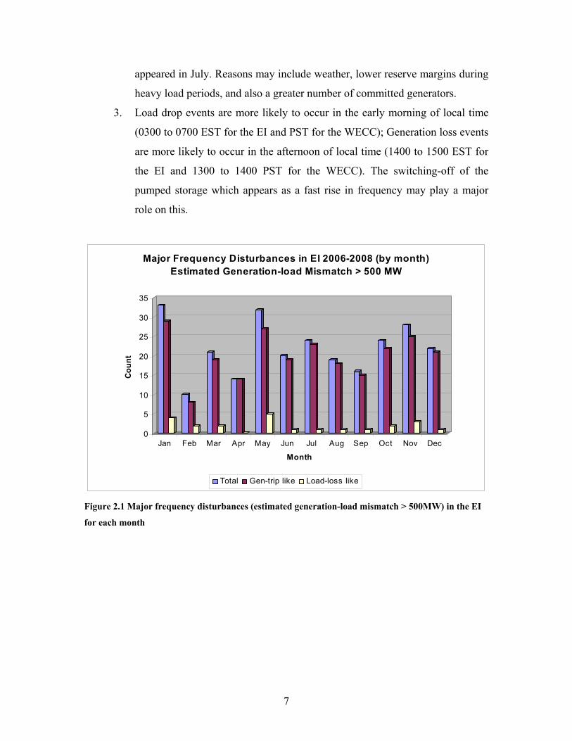
appeared in July. Reasons may include weather, lower reserve margins during
heavy load periods, and also a greater number of committed generators.
3. Load drop events are more likely to occur in the early morning of local time
(0300 to 0700 EST for the EI and PST for the WECC); Generation loss events
are more likely to occur in the afternoon of local time (1400 to 1500 EST for
the EI and 1300 to 1400 PST for the WECC). The switching-off of the
pumped storage which appears as a fast rise in frequency may play a major
role on this.
0
5
10
15
20
25
30
35
Coun
t
Jan Feb Mar Apr May Jun Jul Aug Sep Oct Nov Dec
Month
Major Frequency Disturbances in EI 2006-2008 (by month)Estimated Generation-load Mismatch > 500 MW
Total Gen-trip like Load-loss like
Figure 2.1 Major frequency disturbances (estimated generation-load mismatch > 500MW) in the EI
for each month
8
0
2
4
6
8
10
12
14
16
18
Cou
nt
0-1 2-3 4-5 6-7 8-9 10-11
12-13
14-15
16-17
18-19
20-21
22-23
Hour (UTC)
Major Frequency Disturbances in EI 2006-2008 (by hour)Estimated Generation-load Mismatch > 500 MW
Gen-trip like Load-loss like
Figure 2.2 Major frequency disturbances (estimated generation-load mismatch > 500MW) in the EI
for each hour
0
10
20
30
40
50
60
Coun
t
Jan Feb Mar Apr May Jun Jul Aug Sep Oct Nov Dec
Month
Major Frequency Disturbances in WECC 2006-2008 (by month)Estimated Generation-load Mismatch > 200 MW
Total Gen-trip like Load-loss like
Figure 2.3 Major frequency disturbances (estimated generation-load mismatch > 200MW) in the
WECC for each month
9
0
5
10
15
20
25
30
35
40
45Co
unt
0-1 2-3 4-5 6-7 8-9 10-11
12-13
14-15
16-17
18-19
20-21
22-23
Hour (UTC)
Major Frequency Disturbances in WECC 2006-2008 (by hour)Estimated Generation-load Mismatch > 200 MW
Gen-trip like Load-loss like
Figure 2.4 Major frequency disturbances (estimated generation-load mismatch > 200MW) in the
WECC for each hour
Some distinct characteristics for events in the two Interconnections can be found
from the diagrams:
1. The peak of all events in the EI occurred in January, while the peak in the
WECC occurred in July.
2. Load drop events in the WECC are more likely to occur in April.
3. Disturbances are more likely to occur between 1400 to 1500 EST in the EI
and the generation loss events are more likely to occur between 0900 to 1500
EST. For the WECC system, the peak of disturbances is between 0400 to
0500 PST. Moreover, the generation loss events are more evenly distributed
over 24 hours in the WECC system.
On average, about every 3 days (739/263), where 739 is the total number of days
and 263 is the total number of identified events in the EI during these days, a major event
(defined as generation-load mismatch > 500 MW) is seen in the EI system. The WECC
system experiences an event (defined as generation-load mismatch > 200 MW) every 1.5
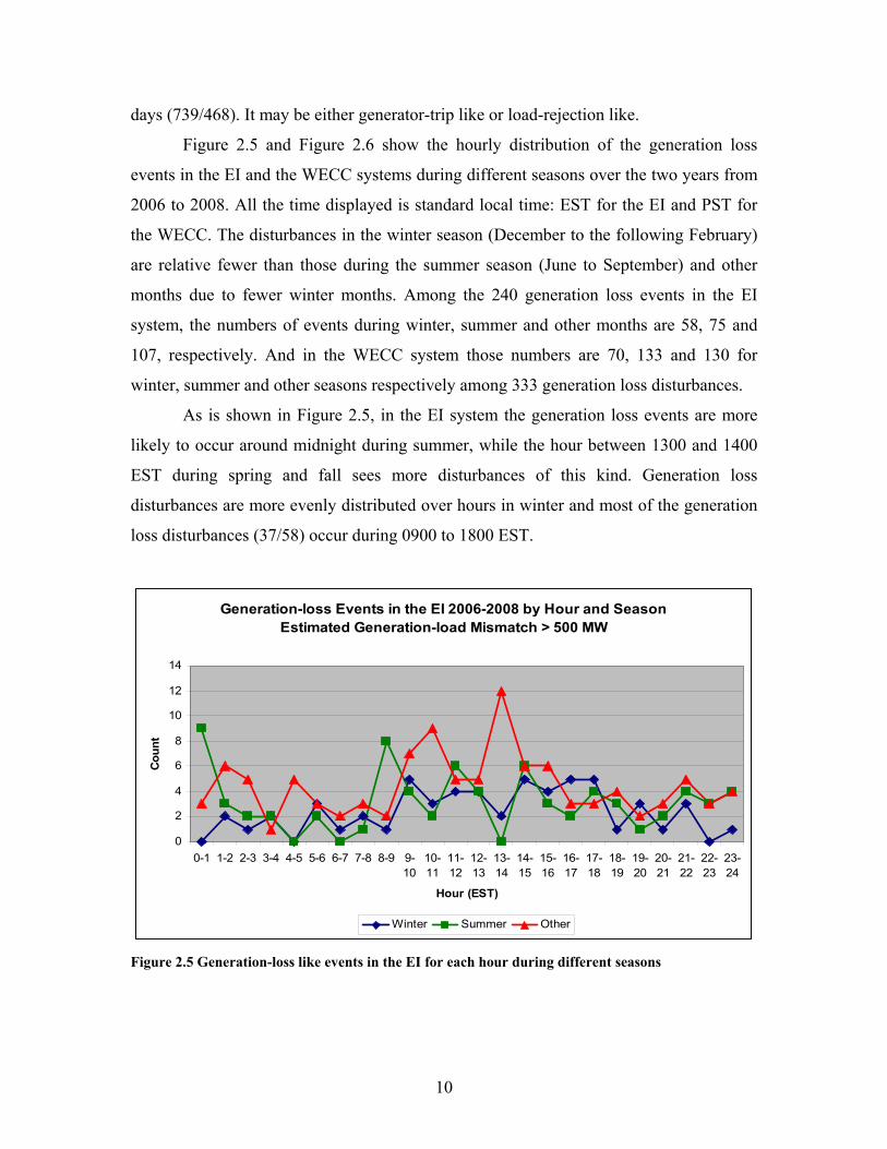
10
days (739/468). It may be either generator-trip like or load-rejection like.
Figure 2.5 and Figure 2.6 show the hourly distribution of the generation loss
events in the EI and the WECC systems during different seasons over the two years from
2006 to 2008. All the time displayed is standard local time: EST for the EI and PST for
the WECC. The disturbances in the winter season (December to the following February)
are relative fewer than those during the summer season (June to September) and other
months due to fewer winter months. Among the 240 generation loss events in the EI
system, the numbers of events during winter, summer and other months are 58, 75 and
107, respectively. And in the WECC system those numbers are 70, 133 and 130 for
winter, summer and other seasons respectively among 333 generation loss disturbances.
As is shown in Figure 2.5, in the EI system the generation loss events are more
likely to occur around midnight during summer, while the hour between 1300 and 1400
EST during spring and fall sees more disturbances of this kind. Generation loss
disturbances are more evenly distributed over hours in winter and most of the generation
loss disturbances (37/58) occur during 0900 to 1800 EST.
Generation-loss Events in the EI 2006-2008 by Hour and Season Estimated Generation-load Mismatch > 500 MW
0
2
4
6
8
10
12
14
0-1 1-2 2-3 3-4 4-5 5-6 6-7 7-8 8-9 9-10
10-11
11-12
12-13
13-14
14-15
15-16
16-17
17-18
18-19
19-20
20-21
21-22
22-23
23-24
Hour (EST)
Coun
t
Winter Summer Other
Figure 2.5 Generation-loss like events in the EI for each hour during different seasons
11
In the WECC system, the generation loss events are more likely to occur between
1100 to 1300 PST in winter and between 1200 to 1400 PST in summer. The disturbances
in the WECC are more evenly distributed during other seasons.
Generation-loss Events in the WECC 2006-2008 by Hour and Season Estimated Generation-load Mismatch > 200 MW
0
2
4
6
8
10
12
14
0-1 1-2 2-3 3-4 4-5 5-6 6-7 7-8 8-9 9-10
10-11
11-12
12-13
13-14
14-15
15-16
16-17
17-18
18-19
19-20
20-21
21-22
22-23
23-24
Hour (PST)
Cou
nt
Winter Summer Other
Figure 2.6 Generation-loss like events in the WECC for each hour during different seasons
In order to compare the hourly variations of the generation loss events during
different seasons for the EI and the WECC, the percentage of the events in each hour to
the total number of events during the season is shown in Figure 2.7 to Figure 2.9. The
comparisons in Figure 2.7 and 2.8 show distinct characteristics of the disturbance
occurrences during winter and summer in the EI and the WECC, which may indicate the
different generation and load profile, reserve distribution and development. For instance,
in summer generation loss events are more likely to occur in the hour 0000 to 0100 EST
in the EI system whereas the peak of such events occurs during 1300 to 1400 PST in the
WECC as shown in Figure 2.8. And no generation loss greater than 500 MW is recorded
during this hour in EST in the EI system. Moreover, higher percentage of the generation
loss disturbances occurs in the summer in the WECC (39.9%) than in the EI (31.2%).
12
Generation-loss Events during Winter in the EI and the WECC by Hour in 2006-2008
0
2
4
6
8
10
12
0-1 1-2 2-3 3-4 4-5 5-6 6-7 7-8 8-9 9-10
10-11
11-12
12-13
13-14
14-15
15-16
16-17
17-18
18-19
19-20
20-21
21-22
22-23
23-24
Hour (EST for EI, PST for WECC)
Perc
enta
ge (%
)
EI Winter WECC Winter
Figure 2.7 Generation-loss like events during winter in the EI and the WECC for each hour
Generation-loss Events during Summer in the EI and the WECC by Hour in 2006-2008
0
2
4
6
8
10
12
14
0-1 1-2 2-3 3-4 4-5 5-6 6-7 7-8 8-9 9-10
10-11
11-12
12-13
13-14
14-15
15-16
16-17
17-18
18-19
19-20
20-21
21-22
22-23
23-24
Hour (EST for EI, PST for Winter)
Perc
enta
ge (%
)
EI Summer WECC Summer
Figure 2.8 Generation-loss like events during summer in the EI and the WECC for each hour
The event distribution by hour in the EI and the WECC demonstrates some
similarities. It can be seen from Figure 2.9 that in spring and fall both the WECC and the
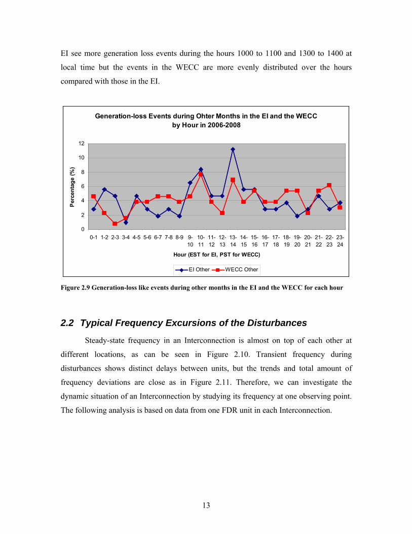
13
EI see more generation loss events during the hours 1000 to 1100 and 1300 to 1400 at
local time but the events in the WECC are more evenly distributed over the hours
compared with those in the EI.
Generation-loss Events during Ohter Months in the EI and the WECC by Hour in 2006-2008
0
2
4
6
8
10
12
0-1 1-2 2-3 3-4 4-5 5-6 6-7 7-8 8-9 9-10
10-11
11-12
12-13
13-14
14-15
15-16
16-17
17-18
18-19
19-20
20-21
21-22
22-23
23-24
Hour (EST for EI, PST for WECC)
Perc
enta
ge (%
)
EI Other WECC Other
Figure 2.9 Generation-loss like events during other months in the EI and the WECC for each hour
2.2 Typical Frequency Excursions of the Disturbances
Steady-state frequency in an Interconnection is almost on top of each other at
different locations, as can be seen in Figure 2.10. Transient frequency during
disturbances shows distinct delays between units, but the trends and total amount of
frequency deviations are close as in Figure 2.11. Therefore, we can investigate the
dynamic situation of an Interconnection by studying its frequency at one observing point.
The following analysis is based on data from one FDR unit in each Interconnection.
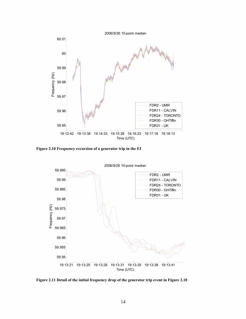
14
19:12:42 19:13:38 19:14:33 19:15:28 19:16:23 19:17:18 19:18:13
59.95
59.96
59.97
59.98
59.99
60
60.01
Time (UTC)
Freq
uenc
y (H
z)
2006/9/26 10-point median
FDR2 - UMRFDR11 - CALVINFDR24 - TORONTOFDR30 - OHTiffinFDR31 - UK
Figure 2.10 Frequency excursion of a generator trip in the EI
19:13:21 19:13:25 19:13:28 19:13:31 19:13:35 19:13:38 19:13:41
59.95
59.955
59.96
59.965
59.97
59.975
59.98
59.985
59.99
59.995
Time (UTC)
Freq
uenc
y (H
z)
2006/9/26 10-point median
FDR2 - UMRFDR11 - CALVINFDR24 - TORONTOFDR30 - OHTiffinFDR31 - UK
Figure 2.11 Detail of the initial frequency drop of the generator trip event in Figure 2.10
15
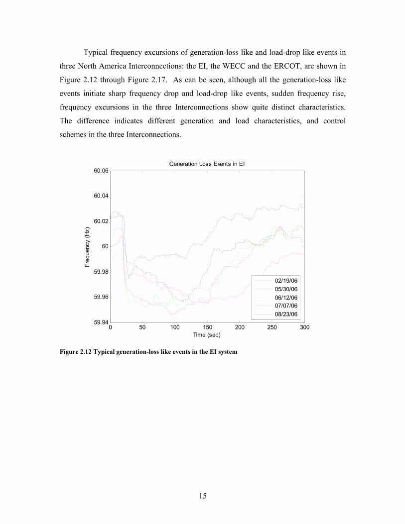
Typical frequency excursions of generation-loss like and load-drop like events in
three North America Interconnections: the EI, the WECC and the ERCOT, are shown in
Figure 2.12 through Figure 2.17. As can be seen, although all the generation-loss like
events initiate sharp frequency drop and load-drop like events, sudden frequency rise,
frequency excursions in the three Interconnections show quite distinct characteristics.
The difference indicates different generation and load characteristics, and control
schemes in the three Interconnections.
Figure 2.12 Typical generation-loss like events in the EI system
0 50 100 150 200 250 30059.94
59.96
59.98
60
60.02
60.04
60.06
Freq
uenc
y (H
z)
Time (sec)
Generation Loss Events in EI
02/19/0605/30/0606/12/0607/07/0608/23/06
16
Figure 2.13 Typical generation-loss like events in the WECC system
Figure 2.14 Typical generation-loss like events in the ERCOT system
0 50 100 150 200 250 30059.7
59.75
59.8
59.85
59.9
59.95
60
60.05
60.1
Freq
uenc
y (H
z)
Time (sec)
Generation Loss Events in ERCOT
08/11/0609/10/0609/28/0610/03/0610/10/06
0 50 100 150 200 250 30059.8
59.85
59.9
59.95
60
60.05
Freq
uenc
y (H
z)
Time (sec)
Generation Loss Events in WECC
03/05/0607/02/0607/26/0610/19/0610/21/06
17
Figure 2.15 Typical load-drop like events in the EI system
Figure 2.16 Typical load-drop like events in the WECC system
0 50 100 150 200 250 300 35059.94
59.96
59.98
60
60.02
60.04
60.06
60.08
60.1
Freq
uenc
y (H
z)
Time (sec)
Load Loss Events in WECC
05/31/0606/12/0606/18/0607/30/0608/19/06
0 50 100 150 200 250 30059.96
59.98
60
60.02
60.04
60.06
60.08
Freq
uenc
y (H
z)
Time (sec)
Load Loss Events in EI
05/05/0605/10/0605/15/0606/13/0608/30/06
18
Figure 2.17 Typical load-drop like events in the ERCOT system
The comparison of frequency excursions of generation-loss like and load-drop
like events in the three Interconnections can be seen in Figure 2.18 and Figure 2.20. The
generation/load loss amount can be estimated from the equation:
fP ∆=∆ β (2.5)
where β is the frequency response characteristic [12] or load-frequency sensitivity
coefficient [13]; f∆ is the total frequency change amount following the disturbance by
12 ssss fff −=∆ , where 1ssf is the pre-disturbance steady state frequency, 2ssf is the post-
disturbance steady state frequency. The amount of frequency change from certain amount
of generation/load loss varies in different Interconnections, because the EI, the WECC
and the ERCOT systems have different β values, which can be found in [12].
0 50 100 150 200 250 300 35059.92
59.94
59.96
59.98
60
60.02
60.04
60.06
60.08
Freq
uenc
y (H
z)
Time (sec)
Load Loss Events in ERCOT
10/21/0610/22/0610/22/0610/22/0610/23/06
19
0 50 100 150 200 250 300 35059.8
59.85
59.9
59.95
60
60.05
Freq
uenc
y (H
z)
Time (sec)
Typical Generation Loss Events in Three Interconnections
EI Estimated Amount:1205MWWECC Estimated Amount:1069MWERCOT Estimated Amount:840MW
Figure 2.18 Generation-loss like events in the three Interconnections
0 10 20 30 40 50 60 70 8059.8
59.85
59.9
59.95
60
60.05
Freq
uenc
y (H
z)
Time (sec)
Typical Generation Loss Events in Three Interconnections
EI Estimated Amount:1205MWWECC Estimated Amount:1069MWERCOT Estimated Amount:840MW
Figure 2.19 Detail of the initial frequency drop for generation-loss like events in the three
Interconnections
20
0 50 100 150 200 250 300 35059.96
59.98
60
60.02
60.04
60.06
60.08
Freq
uenc
y (H
z)
Time (sec)
Typical Generation Loss Events in Three Interconnections
EI Estimated Amount:1050MWWECC Estimated Amount:520MWERCOT Estimated Amount:253MW
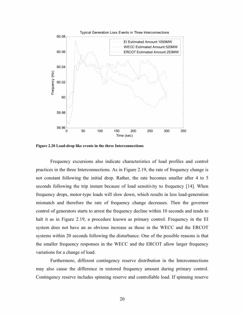
Figure 2.20 Load-drop like events in the three Interconnections
Frequency excursions also indicate characteristics of load profiles and control
practices in the three Interconnections. As in Figure 2.19, the rate of frequency change is
not constant following the initial drop. Rather, the rate becomes smaller after 4 to 5
seconds following the trip instant because of load sensitivity to frequency [14]. When
frequency drops, motor-type loads will slow down, which results in less load-generation
mismatch and therefore the rate of frequency change decreases. Then the governor
control of generators starts to arrest the frequency decline within 10 seconds and tends to
halt it as in Figure 2.19, a procedure known as primary control. Frequency in the EI
system does not have an as obvious increase as those in the WECC and the ERCOT
systems within 20 seconds following the disturbance. One of the possible reasons is that
the smaller frequency responses in the WECC and the ERCOT allow larger frequency
variations for a change of load.
Furthermore, different contingency reserve distribution in the Interconnections
may also cause the difference in restored frequency amount during primary control.
Contingency reserve includes spinning reserve and controllable load. If spinning reserve
21
is the first option, the type of generating units will decide the response time. Comparison
shows that gas-fired and hydro units have faster response time than coal-fired units. Gas
and hydro turbines also have higher ramp rates than coal-fired units [15]. In the WECC
system, the largest part of capacity is hydro-type. And in the ERCOT system, gas-fired
capacity constitutes most of its total capacity [16], [17]. If contingency reserve in the
WECC and the ERCOT consists of large portion of hydro or gas-fired units, those units
will response fast to pick up the frequency drop, which will also contribute to the obvious
frequency rise following its initial dip.
Governor control can bring frequency back to some extent but it does not
necessarily recover frequency to the pre-disturbance level. The Automatic Generation
Control (AGC) actions and reserve development, known as secondary control, continue
to recover the frequency by replacing the amount of lost generation, which generally
takes 5 to 15 minutes. The detailed discussion about secondary control performances of
the three interconnections is in section 2.5.
2.3 Relationship between Frequency Change Rate and Total
Frequency Variation Amount
As discussed above, generation loss introduces steep frequency decline. The
answers to questions such as how much and how fast the frequency drops, and how they
relate to the generation loss amount help us better understand power system dynamics
and therefore improve control measures. In this section, generation loss events are
considered to investigate the relationship between the rate of frequency change and total
frequency deviation amount.
Consider an M generator system shown in Figure 2.21. When there is any
generation-load imbalance, the motion of each generator rotor is governed by the swing
equation as in (2.4):
dtdHPP
sem
ωω2
=−
where H is the rotor inertia constant, and sω is the system synchronous angular velocity.
For a single generator, the imbalance between its mechanical and electrical power output
is proportional to the rate of frequency change.
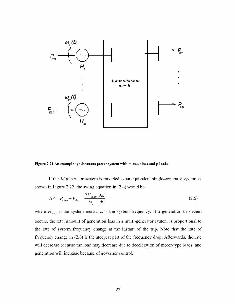
22
Figure 2.21 An example synchronous power system with m machines and p loads
If the M generator system is modeled as an equivalent single-generator system as
shown in Figure 2.22, the swing equation in (2.4) would be:
dtdH
PPPs
equivelecmech
ωω
2=−=∆ (2.6)
where equivH is the system inertia, ω is the system frequency. If a generation trip event
occurs, the total amount of generation loss in a multi-generator system is proportional to
the rate of system frequency change at the instant of the trip. Note that the rate of
frequency change in (2.6) is the steepest part of the frequency drop. Afterwards, the rate
will decrease because the load may decrease due to deceleration of motor-type loads, and
generation will increase because of governor control.
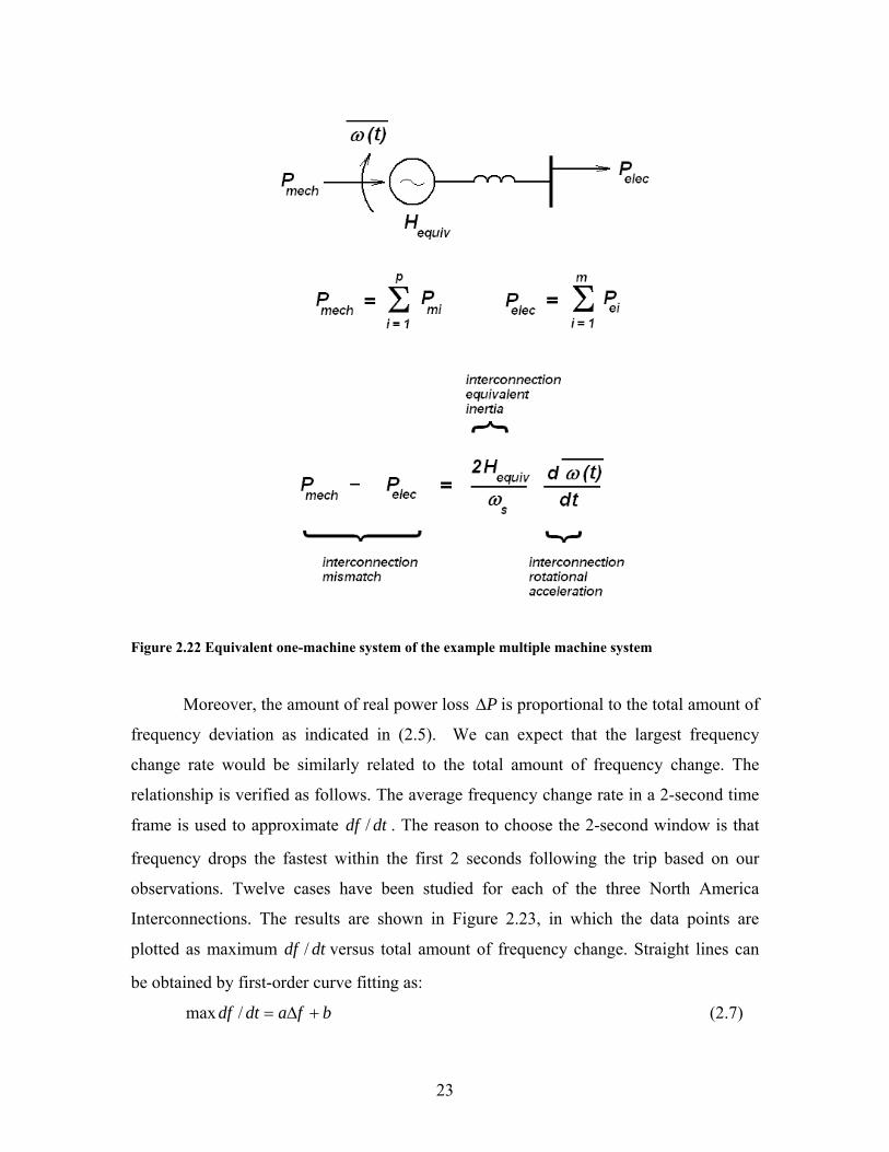
23
Figure 2.22 Equivalent one-machine system of the example multiple machine system
Moreover, the amount of real power loss P∆ is proportional to the total amount of
frequency deviation as indicated in (2.5). We can expect that the largest frequency
change rate would be similarly related to the total amount of frequency change. The
relationship is verified as follows. The average frequency change rate in a 2-second time
frame is used to approximate dtdf / . The reason to choose the 2-second window is that
frequency drops the fastest within the first 2 seconds following the trip based on our
observations. Twelve cases have been studied for each of the three North America
Interconnections. The results are shown in Figure 2.23, in which the data points are
plotted as maximum dtdf / versus total amount of frequency change. Straight lines can
be obtained by first-order curve fitting as:
bfadtdf +∆=/max (2.7)
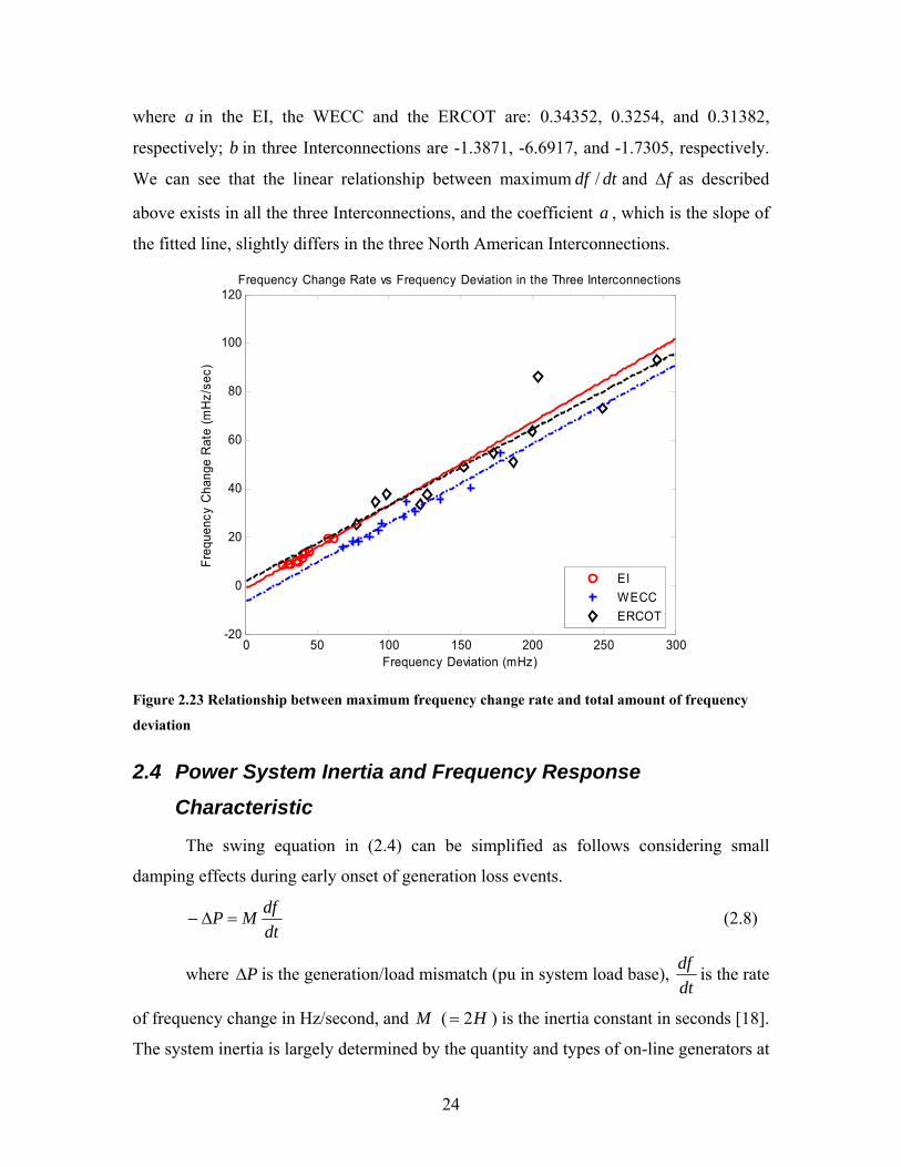
24
where a in the EI, the WECC and the ERCOT are: 0.34352, 0.3254, and 0.31382,
respectively; b in three Interconnections are -1.3871, -6.6917, and -1.7305, respectively.
We can see that the linear relationship between maximum dtdf / and f∆ as described
above exists in all the three Interconnections, and the coefficient a , which is the slope of
the fitted line, slightly differs in the three North American Interconnections.
0 50 100 150 200 250 300-20
0
20
40
60
80
100
120
Frequency Deviation (mHz)
Freq
uenc
y C
hang
e R
ate
(mH
z/se
c)
Frequency Change Rate vs Frequency Deviation in the Three Interconnections
EIWECCERCOT
Figure 2.23 Relationship between maximum frequency change rate and total amount of frequency
deviation
2.4 Power System Inertia and Frequency Response
Characteristic
The swing equation in (2.4) can be simplified as follows considering small
damping effects during early onset of generation loss events.
dtdfMP =∆− (2.8)
where P∆ is the generation/load mismatch (pu in system load base), dtdf is the rate
of frequency change in Hz/second, and M ( H2= ) is the inertia constant in seconds [18].
The system inertia is largely determined by the quantity and types of on-line generators at
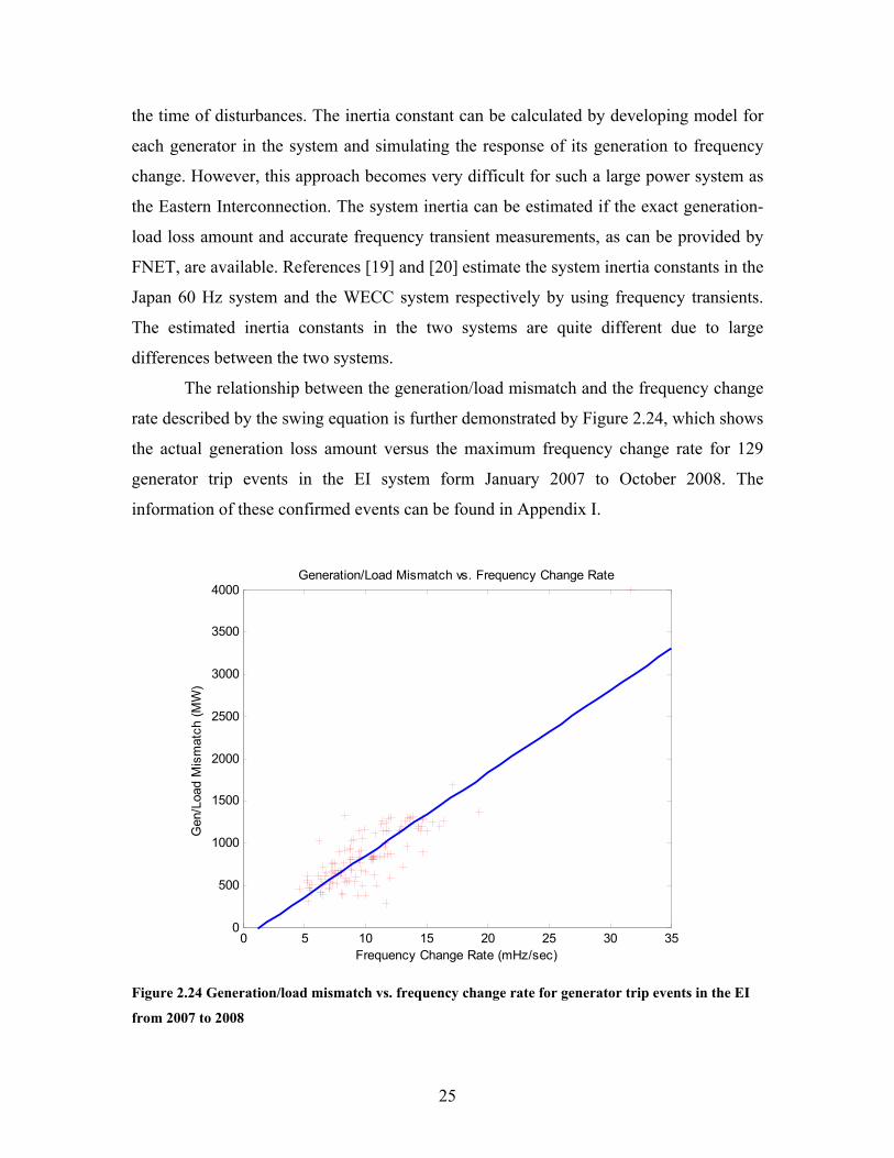
25
the time of disturbances. The inertia constant can be calculated by developing model for
each generator in the system and simulating the response of its generation to frequency
change. However, this approach becomes very difficult for such a large power system as
the Eastern Interconnection. The system inertia can be estimated if the exact generation-
load loss amount and accurate frequency transient measurements, as can be provided by
FNET, are available. References [19] and [20] estimate the system inertia constants in the
Japan 60 Hz system and the WECC system respectively by using frequency transients.
The estimated inertia constants in the two systems are quite different due to large
differences between the two systems.
The relationship between the generation/load mismatch and the frequency change
rate described by the swing equation is further demonstrated by Figure 2.24, which shows
the actual generation loss amount versus the maximum frequency change rate for 129
generator trip events in the EI system form January 2007 to October 2008. The
information of these confirmed events can be found in Appendix I.
0 5 10 15 20 25 30 350
500
1000
1500
2000
2500
3000
3500
4000Generation/Load Mismatch vs. Frequency Change Rate
Gen
/Loa
d M
ism
atch
(MW
)
Frequency Change Rate (mHz/sec)
Figure 2.24 Generation/load mismatch vs. frequency change rate for generator trip events in the EI
from 2007 to 2008
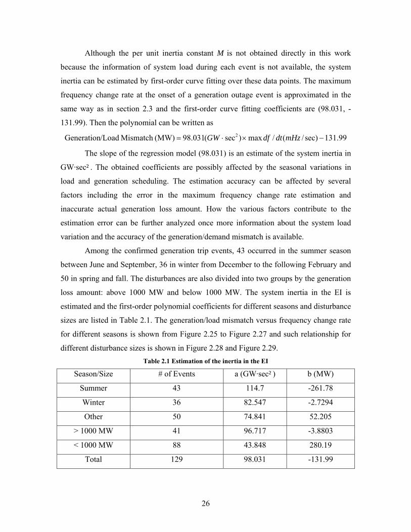
26
Although the per unit inertia constant M is not obtained directly in this work
because the information of system load during each event is not available, the system
inertia can be estimated by first-order curve fitting over these data points. The maximum
frequency change rate at the onset of a generation outage event is approximated in the
same way as in section 2.3 and the first-order curve fitting coefficients are (98.031, -
131.99). Then the polynomial can be written as
131.99sec)/(/max)sec(031.89(MW)Mismatch /LoadGeneration 2 −×⋅= mHzdtdfGW
The slope of the regression model (98.031) is an estimate of the system inertia in
GW·sec². The obtained coefficients are possibly affected by the seasonal variations in
load and generation scheduling. The estimation accuracy can be affected by several
factors including the error in the maximum frequency change rate estimation and
inaccurate actual generation loss amount. How the various factors contribute to the
estimation error can be further analyzed once more information about the system load
variation and the accuracy of the generation/demand mismatch is available.
Among the confirmed generation trip events, 43 occurred in the summer season
between June and September, 36 in winter from December to the following February and
50 in spring and fall. The disturbances are also divided into two groups by the generation
loss amount: above 1000 MW and below 1000 MW. The system inertia in the EI is
estimated and the first-order polynomial coefficients for different seasons and disturbance
sizes are listed in Table 2.1. The generation/load mismatch versus frequency change rate
for different seasons is shown from Figure 2.25 to Figure 2.27 and such relationship for
different disturbance sizes is shown in Figure 2.28 and Figure 2.29. Table 2.1 Estimation of the inertia in the EI
Season/Size # of Events a (GW·sec²) b (MW)
Summer 43 114.7 -261.78
Winter 36 82.547 -2.7294
Other 50 74.841 52.205
> 1000 MW 41 96.717 -3.8803
< 1000 MW 88 43.848 280.19
Total 129 98.031 -131.99
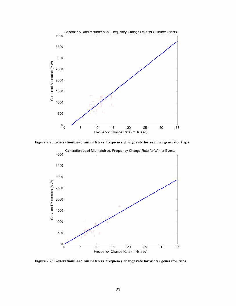
27
0 5 10 15 20 25 30 350
500
1000
1500
2000
2500
3000
3500
4000Generation/Load Mismatch vs. Frequency Change Rate for Summer Events
Gen
/Loa
d M
ism
atch
(MW
)
Frequency Change Rate (mHz/sec)
Figure 2.25 Generation/Load mismatch vs. frequency change rate for summer generator trips
0 5 10 15 20 25 30 350
500
1000
1500
2000
2500
3000
3500
4000Generation/Load Mismatch vs. Frequency Change Rate for Winter Events
Gen
/Loa
d M
ism
atch
(MW
)
Frequency Change Rate (mHz/sec)
Figure 2.26 Generation/Load mismatch vs. frequency change rate for winter generator trips
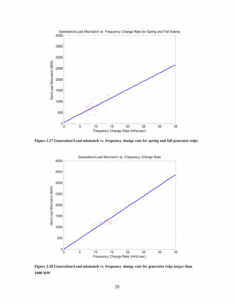
28
0 5 10 15 20 25 30 350
500
1000
1500
2000
2500
3000
3500
4000Generation/Load Mismatch vs. Frequency Change Rate for Spring and Fall Events
Gen
/Loa
d M
ism
atch
(MW
)
Frequency Change Rate (mHz/sec)
Figure 2.27 Generation/Load mismatch vs. frequency change rate for spring and fall generator trips
0 5 10 15 20 25 30 350
500
1000
1500
2000
2500
3000
3500
4000Generation/Load Mismatch vs. Frequency Change Rate
Gen
/Loa
d M
ism
atch
(MW
)
Frequency Change Rate (mHz/sec)
Figure 2.28 Generation/Load mismatch vs. frequency change rate for generator trips larger than
1000 MW
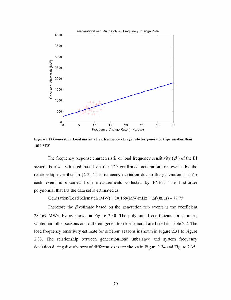
29
0 5 10 15 20 25 30 350
500
1000
1500
2000
2500
3000
3500
4000Generation/Load Mismatch vs. Frequency Change Rate
Gen
/Loa
d M
ism
atch
(MW
)
Frequency Change Rate (mHz/sec)
Figure 2.29 Generation/Load mismatch vs. frequency change rate for generator trips smaller than
1000 MW
The frequency response characteristic or load frequency sensitivity (β ) of the EI
system is also estimated based on the 129 confirmed generation trip events by the
relationship described in (2.5). The frequency deviation due to the generation loss for
each event is obtained from measurements collected by FNET. The first-order
polynomial that fits the data set is estimated as
77.75 )(mHz)28.169(MW/(MW)Mismatch /LoadGeneration −∆×= mHzf
Therefore the β estimate based on the generation trip events is the coefficient
28.169 MW/mHz as shown in Figure 2.30. The polynomial coefficients for summer,
winter and other seasons and different generation loss amount are listed in Table 2.2. The
load frequency sensitivity estimate for different seasons is shown in Figure 2.31 to Figure
2.33. The relationship between generation/load unbalance and system frequency
deviation during disturbances of different sizes are shown in Figure 2.34 and Figure 2.35.
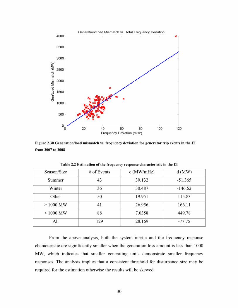
30
0 20 40 60 80 100 1200
500
1000
1500
2000
2500
3000
3500
4000Generation/Load Mismatch vs. Total Frequency Deviation
Frequency Deviation (mHz)
Gen
/Loa
d M
ism
atch
(MW
)
Figure 2.30 Generation/load mismatch vs. frequency deviation for generator trip events in the EI
from 2007 to 2008
Table 2.2 Estimation of the frequency response characteristic in the EI
Season/Size # of Events c (MW/mHz) d (MW)
Summer 43 30.132 -51.365
Winter 36 30.487 -146.62
Other 50 19.951 115.83
> 1000 MW 41 26.956 166.11
< 1000 MW 88 7.0358 449.78
All 129 28.169 -77.75
From the above analysis, both the system inertia and the frequency response
characteristic are significantly smaller when the generation loss amount is less than 1000
MW, which indicates that smaller generating units demonstrate smaller frequency
responses. The analysis implies that a consistent threshold for disturbance size may be
required for the estimation otherwise the results will be skewed.
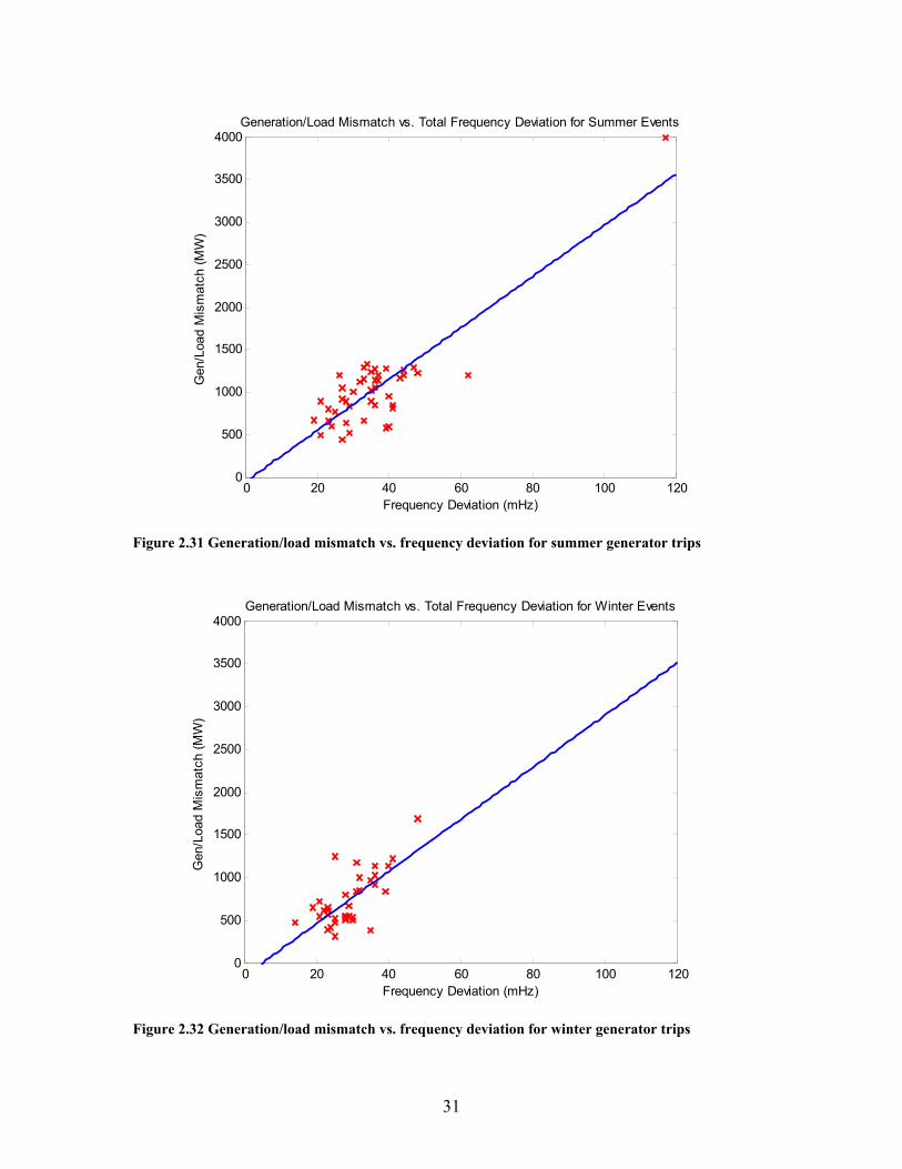
31
0 20 40 60 80 100 1200
500
1000
1500
2000
2500
3000
3500
4000Generation/Load Mismatch vs. Total Frequency Deviation for Summer Events
Frequency Deviation (mHz)
Gen
/Loa
d M
ism
atch
(MW
)
Figure 2.31 Generation/load mismatch vs. frequency deviation for summer generator trips
0 20 40 60 80 100 1200
500
1000
1500
2000
2500
3000
3500
4000Generation/Load Mismatch vs. Total Frequency Deviation for Winter Events
Frequency Deviation (mHz)
Gen
/Loa
d M
ism
atch
(MW
)
Figure 2.32 Generation/load mismatch vs. frequency deviation for winter generator trips
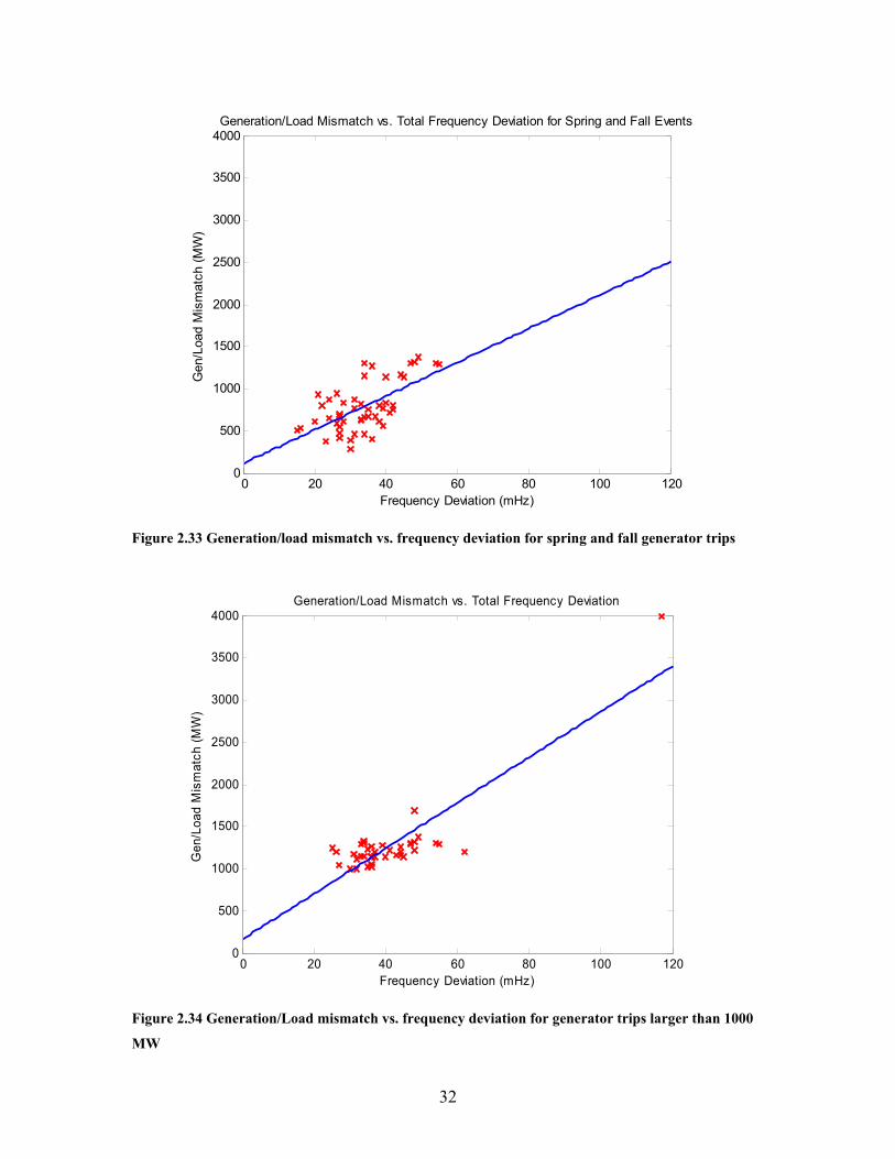
32
0 20 40 60 80 100 1200
500
1000
1500
2000
2500
3000
3500
4000Generation/Load Mismatch vs. Total Frequency Deviation for Spring and Fall Events
Frequency Deviation (mHz)
Gen
/Loa
d M
ism
atch
(MW
)
Figure 2.33 Generation/load mismatch vs. frequency deviation for spring and fall generator trips
0 20 40 60 80 100 1200
500
1000
1500
2000
2500
3000
3500
4000Generation/Load Mismatch vs. Total Frequency Deviation
Frequency Deviation (mHz)
Gen
/Loa
d M
ism
atch
(MW
)
Figure 2.34 Generation/Load mismatch vs. frequency deviation for generator trips larger than 1000
MW
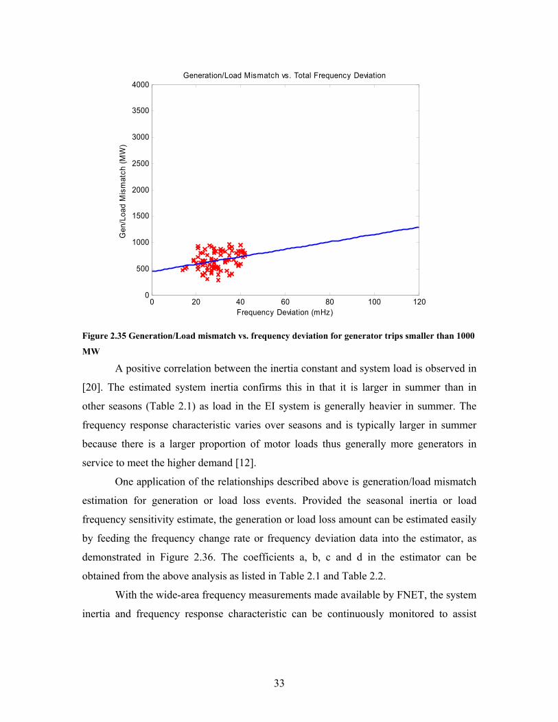
33
0 20 40 60 80 100 1200
500
1000
1500
2000
2500
3000
3500
4000Generation/Load Mismatch vs. Total Frequency Deviation
Frequency Deviation (mHz)
Gen
/Loa
d M
ism
atch
(MW
)
Figure 2.35 Generation/Load mismatch vs. frequency deviation for generator trips smaller than 1000
MW
A positive correlation between the inertia constant and system load is observed in
[20]. The estimated system inertia confirms this in that it is larger in summer than in
other seasons (Table 2.1) as load in the EI system is generally heavier in summer. The
frequency response characteristic varies over seasons and is typically larger in summer
because there is a larger proportion of motor loads thus generally more generators in
service to meet the higher demand [12].
One application of the relationships described above is generation/load mismatch
estimation for generation or load loss events. Provided the seasonal inertia or load
frequency sensitivity estimate, the generation or load loss amount can be estimated easily
by feeding the frequency change rate or frequency deviation data into the estimator, as
demonstrated in Figure 2.36. The coefficients a, b, c and d in the estimator can be
obtained from the above analysis as listed in Table 2.1 and Table 2.2.
With the wide-area frequency measurements made available by FNET, the system
inertia and frequency response characteristic can be continuously monitored to assist
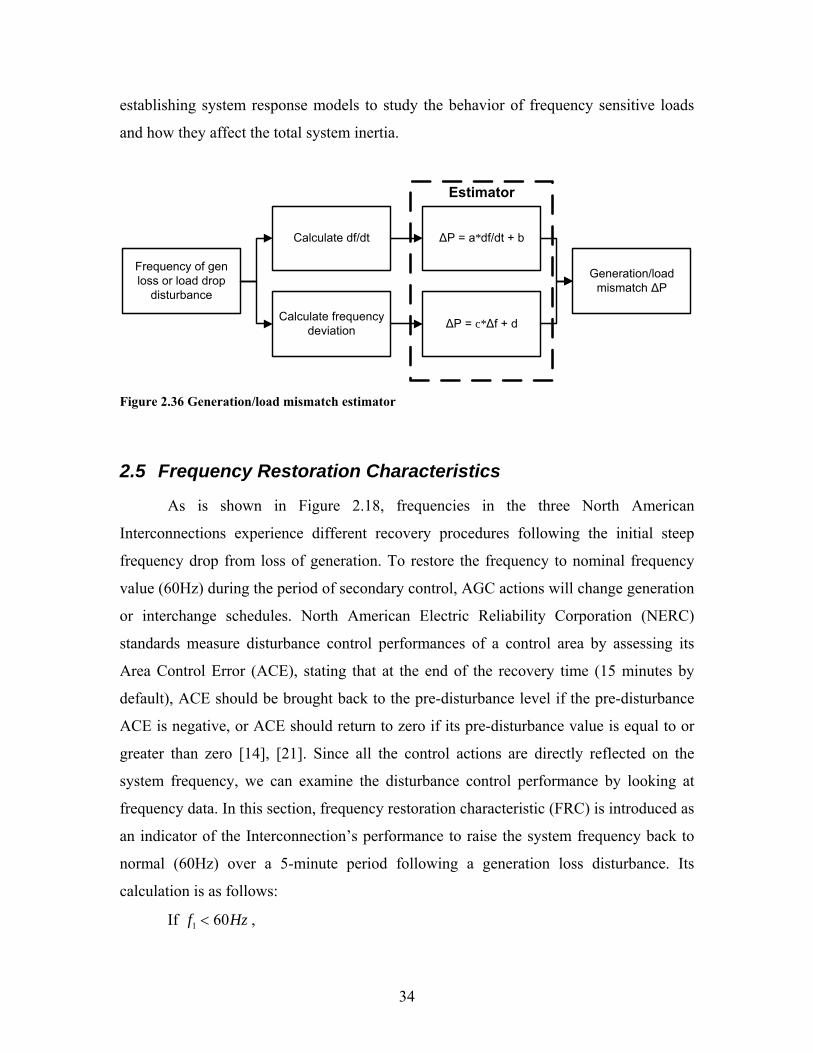
34
establishing system response models to study the behavior of frequency sensitive loads
and how they affect the total system inertia.
Frequency of gen loss or load drop
disturbance
Calculate df/dt
Calculate frequency deviation
∆P = a*df/dt + b
∆P = c*∆f + d
Generation/load mismatch ∆P
Estimator
Figure 2.36 Generation/load mismatch estimator
2.5 Frequency Restoration Characteristics
As is shown in Figure 2.18, frequencies in the three North American
Interconnections experience different recovery procedures following the initial steep
frequency drop from loss of generation. To restore the frequency to nominal frequency
value (60Hz) during the period of secondary control, AGC actions will change generation
or interchange schedules. North American Electric Reliability Corporation (NERC)
standards measure disturbance control performances of a control area by assessing its
Area Control Error (ACE), stating that at the end of the recovery time (15 minutes by
default), ACE should be brought back to the pre-disturbance level if the pre-disturbance
ACE is negative, or ACE should return to zero if its pre-disturbance value is equal to or
greater than zero [14], [21]. Since all the control actions are directly reflected on the
system frequency, we can examine the disturbance control performance by looking at
frequency data. In this section, frequency restoration characteristic (FRC) is introduced as
an indicator of the Interconnection’s performance to raise the system frequency back to
normal (60Hz) over a 5-minute period following a generation loss disturbance. Its
calculation is as follows:
If Hzf 601 < ,
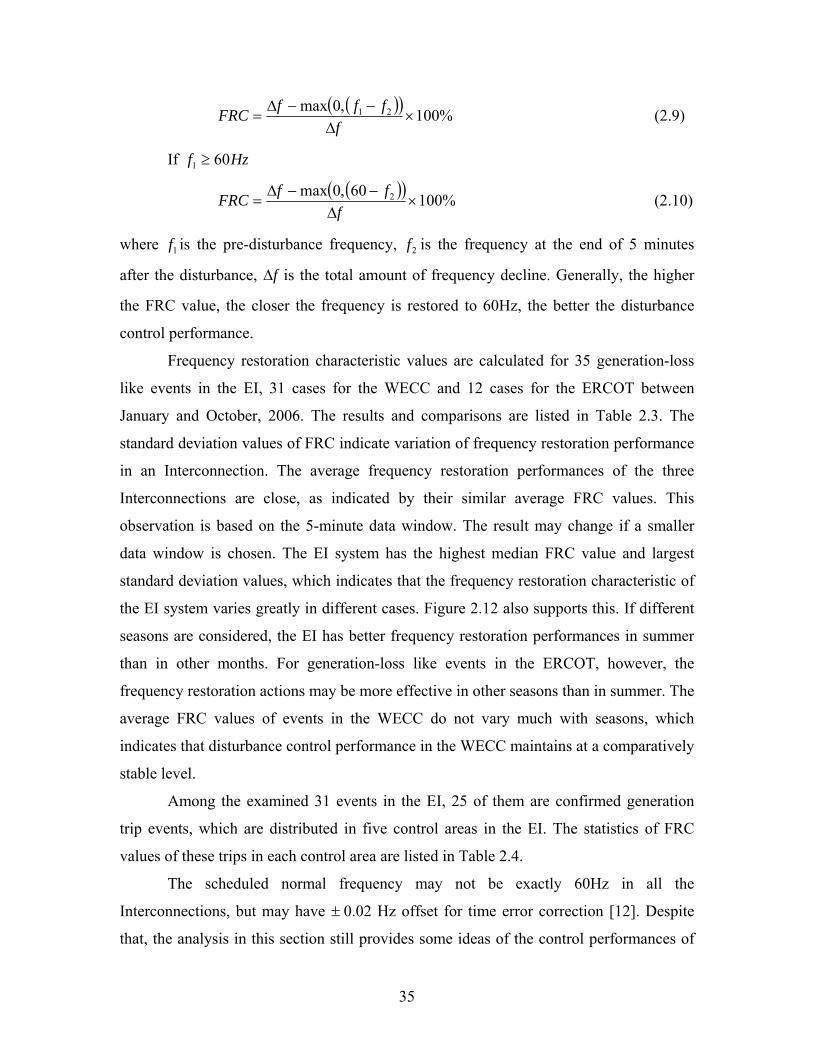
35
( )( ) %100,0max 21 ×∆
−−∆=
ffffFRC (2.9)
If Hzf 601 ≥
( )( ) %10060,0max 2 ×∆
−−∆=
fffFRC (2.10)
where 1f is the pre-disturbance frequency, 2f is the frequency at the end of 5 minutes
after the disturbance, f∆ is the total amount of frequency decline. Generally, the higher
the FRC value, the closer the frequency is restored to 60Hz, the better the disturbance
control performance.
Frequency restoration characteristic values are calculated for 35 generation-loss
like events in the EI, 31 cases for the WECC and 12 cases for the ERCOT between
January and October, 2006. The results and comparisons are listed in Table 2.3. The
standard deviation values of FRC indicate variation of frequency restoration performance
in an Interconnection. The average frequency restoration performances of the three
Interconnections are close, as indicated by their similar average FRC values. This
observation is based on the 5-minute data window. The result may change if a smaller
data window is chosen. The EI system has the highest median FRC value and largest
standard deviation values, which indicates that the frequency restoration characteristic of
the EI system varies greatly in different cases. Figure 2.12 also supports this. If different
seasons are considered, the EI has better frequency restoration performances in summer
than in other months. For generation-loss like events in the ERCOT, however, the
frequency restoration actions may be more effective in other seasons than in summer. The
average FRC values of events in the WECC do not vary much with seasons, which
indicates that disturbance control performance in the WECC maintains at a comparatively
stable level.
Among the examined 31 events in the EI, 25 of them are confirmed generation
trip events, which are distributed in five control areas in the EI. The statistics of FRC
values of these trips in each control area are listed in Table 2.4.
The scheduled normal frequency may not be exactly 60Hz in all the
Interconnections, but may have ± 0.02 Hz offset for time error correction [12]. Despite
that, the analysis in this section still provides some ideas of the control performances of
36
Interconnections as well as control areas. The frequency restoration characteristic can still
serve as an indicator of the reliability of an Interconnection.
Table 2.3 Statistics of frequency restoration characteristic of generation-loss like events in the three
Interconnections from Jan. to Oct. 2006
Interconnection Number of
cases
FRC
average (%)
FRC
median (%)
FRC standard
deviation
Total
EI 35 84.21 100 27.77
WECC 31 84.22 89.08 16.91
ERCOT 12 89.47 95.1 12.42
Summer (Jun. to Sep.)
EI 15 90.83 100 19.73
WECC 12 82.7 93 22.29
ERCOT 5 83.63 80.8 10.15
Other months (Mar. to May, Oct.)
EI 18 76.93 99.25 33.128
WECC 14 83.39 85.21 13.73
ERCOT 7 93.65 100 12.86
Table 2.4 Statistics of frequency restoration characteristic of some generation trips in the EI control
areas
Control Area Number of cases FRC average (%) FRC median (%)
ECAR 7 86.41 100
MAAC 2 81.22 81.22
NPCC 1 98.51 98.51
SERC 12 75.41 84.49
SPP 3 100 100
37
Chapter 3 Analysis of Major Disturbances in the Eastern Interconnection
Power systems are continuously exposed to disturbances whose impacts on the
whole system may vary. Statistical analysis in section 2.1.1 shows that every 3 days
FNET sees a disturbance in EI in which the estimated generation-load mismatch exceeds
500 MW. During a disturbance (generation trip, load loss or line trip) where generation
and load are not balanced, generators in the system accelerate or decelerate to reduce the
power imbalance. Local phase angle and frequency will change simultaneously in
response to the disturbance [10]. Therefore, by monitoring those parameters, valuable
information about system dynamics can be obtained. A situation awareness system has
been implemented on the FNET server to detect and analyze power system disturbances
in near-real time [9].
This section discusses several major disturbances in the EI observed by FNET in
year 2007 and 2008 including a three-phase fault at transmission level, a multiple-
disturbance incident that involves line trips and generator trips, an islanding event, the
Florida outage, HVDC line faults, and events showing the dynamic performance of
AC/DC systems. Frequency, voltage and phase angle recordings are examined to study
the system dynamics during disturbances and understand the signatures of different types
of events. Comparisons of data from PMU and FDR are also included to evaluate data
quality measured at distribution voltage level.
3.1 Three-phase Fault
In summer 2007 a three-phase fault at transmission network triggered the
situation awareness system of FNET. The fault occurred at 00:28:42 UTC, and was
cleared after 23 cycles. An estimation of 800 MW load loss occurred at 00:28:52 UTC.
The measurements from 7 FDR units at different locations are shown in Figure
3.1 through Figure 3.4. For the ease of comparison, voltage at each measuring point is
normalized by dividing by a base voltage which is the average pre-event value over a 20-
second time period at that measuring point. The phase angles at all locations are scaled to
start at zero to eliminate arbitrary angle offsets caused by phase shift from transmission to
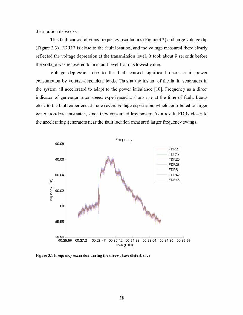
38
distribution networks.
This fault caused obvious frequency oscillations (Figure 3.2) and large voltage dip
(Figure 3.3). FDR17 is close to the fault location, and the voltage measured there clearly
reflected the voltage depression at the transmission level. It took about 9 seconds before
the voltage was recovered to pre-fault level from its lowest value.
Voltage depression due to the fault caused significant decrease in power
consumption by voltage-dependent loads. Thus at the instant of the fault, generators in
the system all accelerated to adapt to the power imbalance [18]. Frequency as a direct
indicator of generator rotor speed experienced a sharp rise at the time of fault. Loads
close to the fault experienced more severe voltage depression, which contributed to larger
generation-load mismatch, since they consumed less power. As a result, FDRs closer to
the accelerating generators near the fault location measured larger frequency swings.
00:25:55 00:27:21 00:28:47 00:30:12 00:31:38 00:33:04 00:34:30 00:35:5559.96
59.98
60
60.02
60.04
60.06
60.08
Time (UTC)
Freq
uenc
y (H
z)
Frequency
FDR2FDR17FDR20FDR23FDR6FDR42FDR43
Figure 3.1 Frequency excursion during the three-phase disturbance
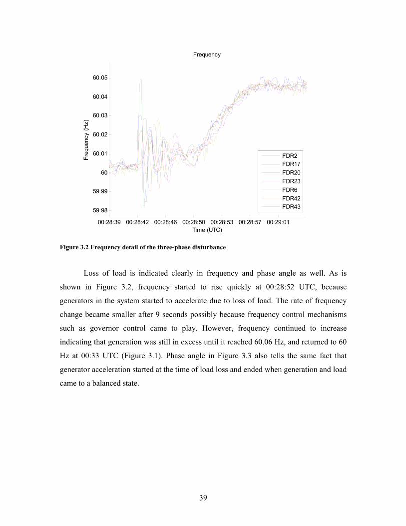
39
00:28:39 00:28:42 00:28:46 00:28:50 00:28:53 00:28:57 00:29:01
59.98
59.99
60
60.01
60.02
60.03
60.04
60.05
Time (UTC)
Freq
uenc
y (H
z)
Frequency
FDR2FDR17FDR20FDR23FDR6FDR42FDR43
Figure 3.2 Frequency detail of the three-phase disturbance
Loss of load is indicated clearly in frequency and phase angle as well. As is
shown in Figure 3.2, frequency started to rise quickly at 00:28:52 UTC, because
generators in the system started to accelerate due to loss of load. The rate of frequency
change became smaller after 9 seconds possibly because frequency control mechanisms
such as governor control came to play. However, frequency continued to increase
indicating that generation was still in excess until it reached 60.06 Hz, and returned to 60
Hz at 00:33 UTC (Figure 3.1). Phase angle in Figure 3.3 also tells the same fact that
generator acceleration started at the time of load loss and ended when generation and load
came to a balanced state.
40
00:26:45 00:28:11 00:29:36 00:31:02 00:32:28 00:33:54 00:35:19 00:36:45-500
0
500
1000
1500
2000
2500
3000
Time (UTC)
Ang
le (d
egre
e)
Voltage Phase Angle
FDR2FDR17FDR20FDR23FDR6FDR42FDR43
Figure 3.3 Phase angle during the three-phase disturbance
00:28:25 00:28:33 00:28:40 00:28:48 00:28:55 00:29:03 00:29:10 00:29:18
0.94
0.95
0.96
0.97
0.98
0.99
1
1.01
1.02
Time (UTC)
Vol
tage
(p.u
.)
Voltage
FDR2FDR17FDR20FDR23FDR6FDR42FDR43
Figure 3.4 Voltage dip caused by the three-phase disturbance
41
3.2 Multi-disturbance Event
Also in summer 2007, FNET event trigger captured a large generation trip event
in EI with about 4000 MW generation loss. It was later confirmed that several generating
units were tripped at that time, and more than one 765 kV transmission lines were
disconnected around the generation trip incident. Although the detailed sequence of
events is still under investigation, much information about what might have happened
during the disturbance can be obtained from real measurements, as is shown in Figure 3.5
to Figure 3.9.
Before the large generation trip, some possible line events occurred between
21:43 UTC and 21:44 UTC (Figure 3.6). Associated with frequency oscillations at
21:43:34 UTC which could be a sign of line trip, a fast frequency decline of about 20
mHz can be noticed, but the frequency returned back fairly quickly. Fast-valving action
at one or more units following the line trip might have contributed to the frequency
decline, which could also explain the frequency’s fast return. It has been found that fast-
valving of units at fault area help minimize the accelerating power and hence reduces
transient power swings by varying the turbine mechanical power [22][23]. Another group
of oscillations can be observed about 15 seconds later, which is possibly due to line re-
closing action that causes similar oscillations in frequency as line opening. The 15-
second delay may be related to the re-closing relay settings.
Immediately before the large frequency decline in Figure 3.7, frequency
oscillations indicate that there might be one or more line trip events. Oscillations in
voltage may also be caused by the line trip events (Figure 3.9). At the onset of a line trip,
generators at sending end of the line will accelerate due to the excessive generation with
respect to load; whereas generators at receiving end of the line will decelerate.
During this disturbance, frequency dropped as low as 59.86 Hz and took 7
minutes to be recovered to 60 Hz (Figure 3.5). Since frequency and phase angle change
simultaneously, phase angle declined after loss of generation, which indicates load was in
excess of generation (Figure 3.8). In addition, the decline did not stop until all lost
generation was replaced by Automatic Generation Control (AGC) and frequency was
restored to its initial equilibrium value.
42
21:40:00 21:42:51 21:45:43 21:48:34 21:51:26 21:54:17 21:57:09 22:00:0059.85
59.9
59.95
60
60.05
60.1
Time (UTC)
Freq
uenc
y (H
z)
Frequency
FDR4FDR38FDR40FDR41FDR42FDR43
Figure 3.5 Frequency excursion during the multi-disturbance event
21:43:24 21:43:29 21:43:35 21:43:40 21:43:45 21:43:50 21:43:56
59.975
59.98
59.985
59.99
59.995
60
60.005
60.01
60.015
Time (UTC)
Freq
uenc
y (H
z)
Frequency
FDR4FDR38FDR40FDR41FDR42FDR43
Figure 3.6 Frequency detail of line events before the generation trip
43
21:44:10 21:44:14 21:44:18 21:44:21 21:44:25 21:44:28 21:44:32 21:44:35
59.88
59.9
59.92
59.94
59.96
59.98
60
60.02
Time (UTC)
Freq
uenc
y (H
z)
Frequency
FDR4FDR38FDR40FDR41FDR42FDR43
Figure 3.7 Frequency detail of the generation trip during the multi-disturbance event
21:40:00 21:42:51 21:45:43 21:48:34 21:51:26 21:54:17 21:57:09 22:00:00-14000
-12000
-10000
-8000
-6000
-4000
-2000
0
2000
Time (UTC)
Ang
le (d
egre
e)
Voltage Phase Angle
FDR4FDR38FDR40FDR41FDR42FDR43
s Figure 3.8 Phase angle during the multi-disturbance event
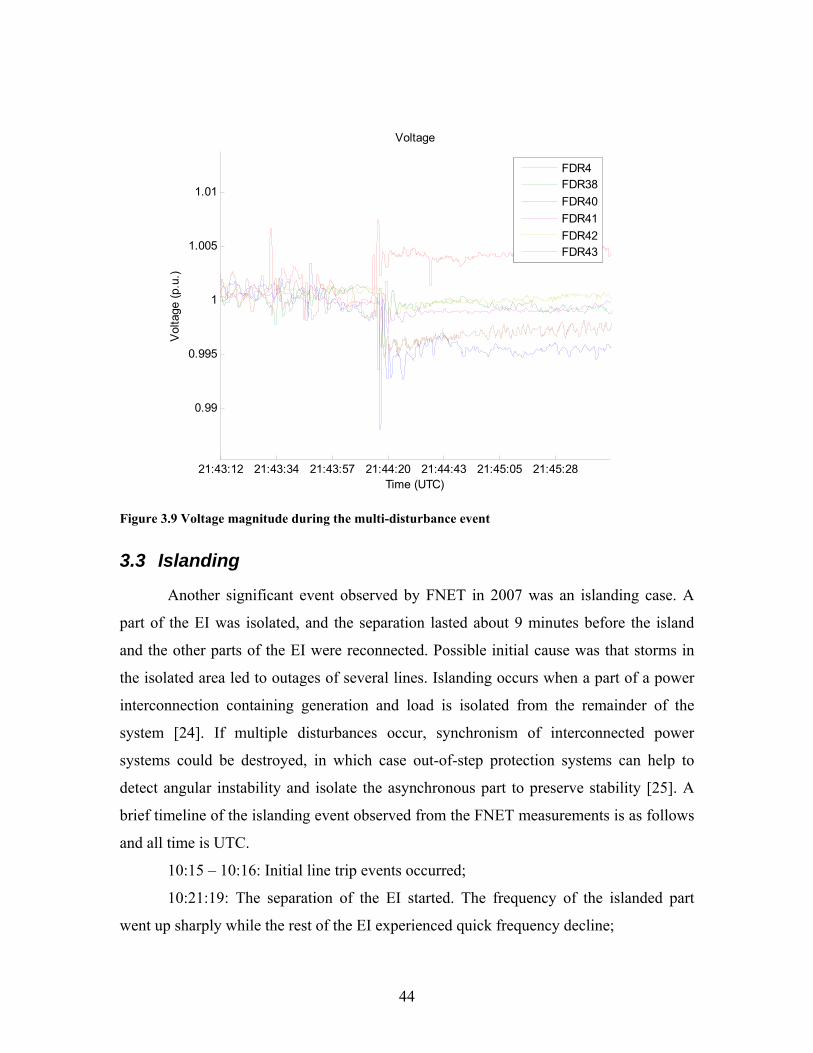
44
21:43:12 21:43:34 21:43:57 21:44:20 21:44:43 21:45:05 21:45:28
0.99
0.995
1
1.005
1.01
Time (UTC)
Vol
tage
(p.u
.)
Voltage
FDR4FDR38FDR40FDR41FDR42FDR43
Figure 3.9 Voltage magnitude during the multi-disturbance event
3.3 Islanding
Another significant event observed by FNET in 2007 was an islanding case. A
part of the EI was isolated, and the separation lasted about 9 minutes before the island
and the other parts of the EI were reconnected. Possible initial cause was that storms in
the isolated area led to outages of several lines. Islanding occurs when a part of a power
interconnection containing generation and load is isolated from the remainder of the
system [24]. If multiple disturbances occur, synchronism of interconnected power
systems could be destroyed, in which case out-of-step protection systems can help to
detect angular instability and isolate the asynchronous part to preserve stability [25]. A
brief timeline of the islanding event observed from the FNET measurements is as follows
and all time is UTC.
10:15 – 10:16: Initial line trip events occurred;
10:21:19: The separation of the EI started. The frequency of the islanded part
went up sharply while the rest of the EI experienced quick frequency decline;
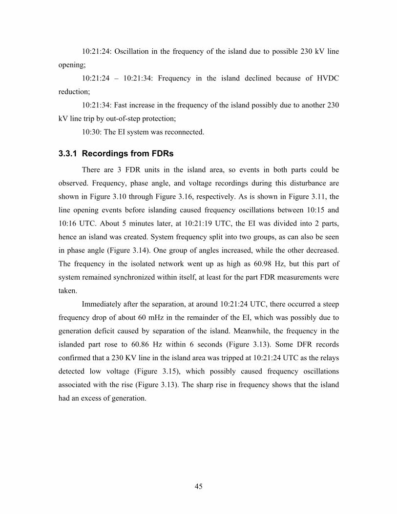
45
10:21:24: Oscillation in the frequency of the island due to possible 230 kV line
opening;
10:21:24 – 10:21:34: Frequency in the island declined because of HVDC
reduction;
10:21:34: Fast increase in the frequency of the island possibly due to another 230
kV line trip by out-of-step protection;
10:30: The EI system was reconnected.
3.3.1 Recordings from FDRs
There are 3 FDR units in the island area, so events in both parts could be
observed. Frequency, phase angle, and voltage recordings during this disturbance are
shown in Figure 3.10 through Figure 3.16, respectively. As is shown in Figure 3.11, the
line opening events before islanding caused frequency oscillations between 10:15 and
10:16 UTC. About 5 minutes later, at 10:21:19 UTC, the EI was divided into 2 parts,
hence an island was created. System frequency split into two groups, as can also be seen
in phase angle (Figure 3.14). One group of angles increased, while the other decreased.
The frequency in the isolated network went up as high as 60.98 Hz, but this part of
system remained synchronized within itself, at least for the part FDR measurements were
taken.
Immediately after the separation, at around 10:21:24 UTC, there occurred a steep
frequency drop of about 60 mHz in the remainder of the EI, which was possibly due to
generation deficit caused by separation of the island. Meanwhile, the frequency in the
islanded part rose to 60.86 Hz within 6 seconds (Figure 3.13). Some DFR records
confirmed that a 230 KV line in the island area was tripped at 10:21:24 UTC as the relays
detected low voltage (Figure 3.15), which possibly caused frequency oscillations
associated with the rise (Figure 3.13). The sharp rise in frequency shows that the island
had an excess of generation.
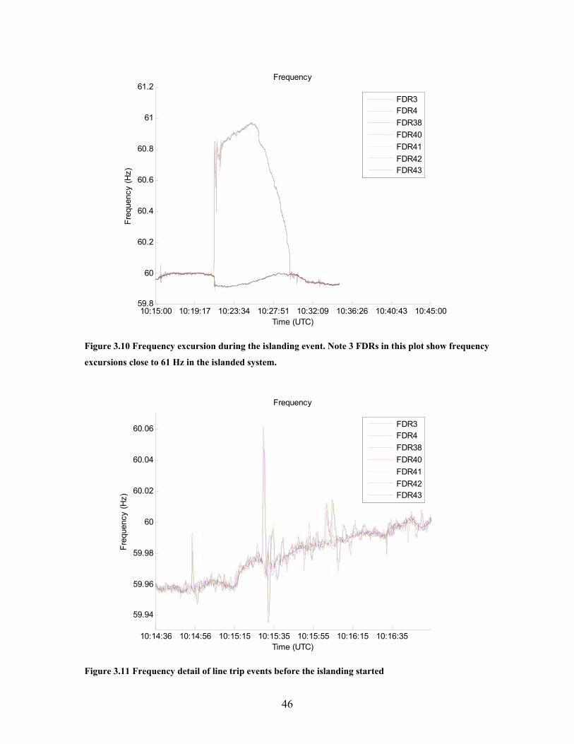
46
10:15:00 10:19:17 10:23:34 10:27:51 10:32:09 10:36:26 10:40:43 10:45:0059.8
60
60.2
60.4
60.6
60.8
61
61.2
Time (UTC)
Freq
uenc
y (H
z)
Frequency
FDR3FDR4FDR38FDR40FDR41FDR42FDR43
Figure 3.10 Frequency excursion during the islanding event. Note 3 FDRs in this plot show frequency
excursions close to 61 Hz in the islanded system.
10:14:36 10:14:56 10:15:15 10:15:35 10:15:55 10:16:15 10:16:35
59.94
59.96
59.98
60
60.02
60.04
60.06
Time (UTC)
Freq
uenc
y (H
z)
Frequency
FDR3FDR4FDR38FDR40FDR41FDR42FDR43
Figure 3.11 Frequency detail of line trip events before the islanding started
47
10:21:18 10:21:21 10:21:25 10:21:28 10:21:32 10:21:35 10:21:39 10:21:42
59.88
59.9
59.92
59.94
59.96
59.98
60
Time (UTC)
Freq
uenc
y (H
z)
Frequency
FDR3FDR4FDR38FDR40FDR41FDR42FDR43
Figure 3.12 Frequency detail showing the start of the islanding - the remainder of the interconnection
10:21:20 10:21:24 10:21:29 10:21:34 10:21:39 10:21:43 10:21:48
60
60.1
60.2
60.3
60.4
60.5
60.6
60.7
60.8
60.9
Time (UTC)
Freq
uenc
y (H
z)
Frequency
FDR3FDR4FDR38FDR40FDR41FDR42FDR43
Figure 3.13 Frequency detail showing the start of the islanding - island
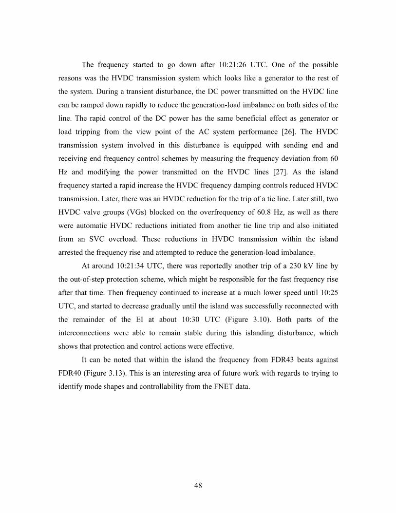
48
The frequency started to go down after 10:21:26 UTC. One of the possible
reasons was the HVDC transmission system which looks like a generator to the rest of
the system. During a transient disturbance, the DC power transmitted on the HVDC line
can be ramped down rapidly to reduce the generation-load imbalance on both sides of the
line. The rapid control of the DC power has the same beneficial effect as generator or
load tripping from the view point of the AC system performance [26]. The HVDC
transmission system involved in this disturbance is equipped with sending end and
receiving end frequency control schemes by measuring the frequency deviation from 60
Hz and modifying the power transmitted on the HVDC lines [27]. As the island
frequency started a rapid increase the HVDC frequency damping controls reduced HVDC
transmission. Later, there was an HVDC reduction for the trip of a tie line. Later still, two
HVDC valve groups (VGs) blocked on the overfrequency of 60.8 Hz, as well as there
were automatic HVDC reductions initiated from another tie line trip and also initiated
from an SVC overload. These reductions in HVDC transmission within the island
arrested the frequency rise and attempted to reduce the generation-load imbalance.
At around 10:21:34 UTC, there was reportedly another trip of a 230 kV line by
the out-of-step protection scheme, which might be responsible for the fast frequency rise
after that time. Then frequency continued to increase at a much lower speed until 10:25
UTC, and started to decrease gradually until the island was successfully reconnected with
the remainder of the EI at about 10:30 UTC (Figure 3.10). Both parts of the
interconnections were able to remain stable during this islanding disturbance, which
shows that protection and control actions were effective.
It can be noted that within the island the frequency from FDR43 beats against
FDR40 (Figure 3.13). This is an interesting area of future work with regards to trying to
identify mode shapes and controllability from the FNET data.
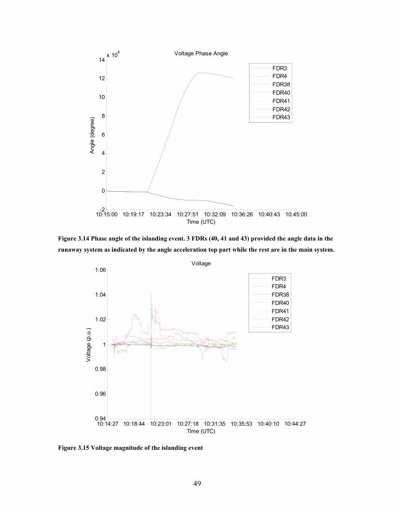
49
10:15:00 10:19:17 10:23:34 10:27:51 10:32:09 10:36:26 10:40:43 10:45:00-2
0
2
4
6
8
10
12
14x 104
Time (UTC)
Ang
le (d
egre
e)
Voltage Phase Angle
FDR3FDR4FDR38FDR40FDR41FDR42FDR43
Figure 3.14 Phase angle of the islanding event. 3 FDRs (40, 41 and 43) provided the angle data in the
runaway system as indicated by the angle acceleration top part while the rest are in the main system.
10:14:27 10:18:44 10:23:01 10:27:18 10:31:35 10:35:53 10:40:10 10:44:270.94
0.96
0.98
1
1.02
1.04
1.06
Time (UTC)
Vol
tage
(p.u
.)
Voltage
FDR3FDR4FDR38FDR40FDR41FDR42FDR43
Figure 3.15 Voltage magnitude of the islanding event
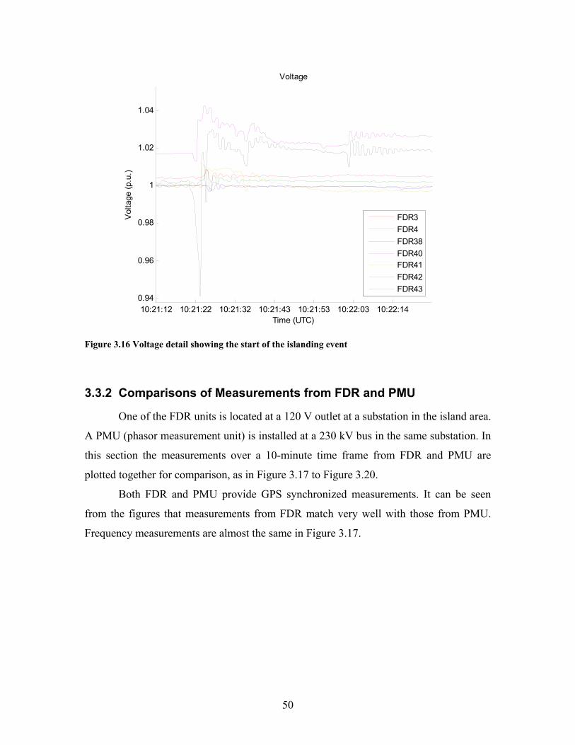
50
10:21:12 10:21:22 10:21:32 10:21:43 10:21:53 10:22:03 10:22:140.94
0.96
0.98
1
1.02
1.04
Time (UTC)
Vol
tage
(p.u
.)
Voltage
FDR3FDR4FDR38FDR40FDR41FDR42FDR43
Figure 3.16 Voltage detail showing the start of the islanding event
3.3.2 Comparisons of Measurements from FDR and PMU
One of the FDR units is located at a 120 V outlet at a substation in the island area.
A PMU (phasor measurement unit) is installed at a 230 kV bus in the same substation. In
this section the measurements over a 10-minute time frame from FDR and PMU are
plotted together for comparison, as in Figure 3.17 to Figure 3.20.
Both FDR and PMU provide GPS synchronized measurements. It can be seen
from the figures that measurements from FDR match very well with those from PMU.
Frequency measurements are almost the same in Figure 3.17.
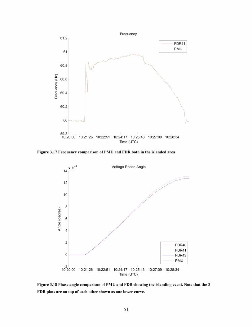
51
10:20:00 10:21:26 10:22:51 10:24:17 10:25:43 10:27:09 10:28:3459.8
60
60.2
60.4
60.6
60.8
61
61.2
Time (UTC)
Freq
uenc
y (H
z)
Frequency
FDR41PMU
Figure 3.17 Frequency comparison of PMU and FDR both in the islanded area
10:20:00 10:21:26 10:22:51 10:24:17 10:25:43 10:27:09 10:28:34-2
0
2
4
6
8
10
12
14x 10
4
Time (UTC)
Ang
le (d
egre
e)
Voltage Phase Angle
FDR40FDR41FDR43PMU
Figure 3.18 Phase angle comparison of PMU and FDR showing the islanding event. Note that the 3
FDR plots are on top of each other shown as one lower curve.
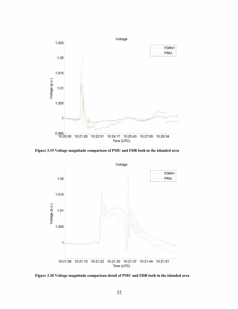
52
10:20:00 10:21:26 10:22:51 10:24:17 10:25:43 10:27:09 10:28:340.995
1
1.005
1.01
1.015
1.02
1.025
Time (UTC)
Vol
tage
(p.u
.)
Voltage
FDR41PMU
Figure 3.19 Voltage magnitude comparison of PMU and FDR both in the islanded area
10:21:08 10:21:15 10:21:22 10:21:30 10:21:37 10:21:44 10:21:51
1
1.005
1.01
1.015
1.02
Time (UTC)
Vol
tage
(p.u
.)
Voltage
FDR41PMU
Figure 3.20 Voltage magnitude comparison detail of PMU and FDR both in the islanded area
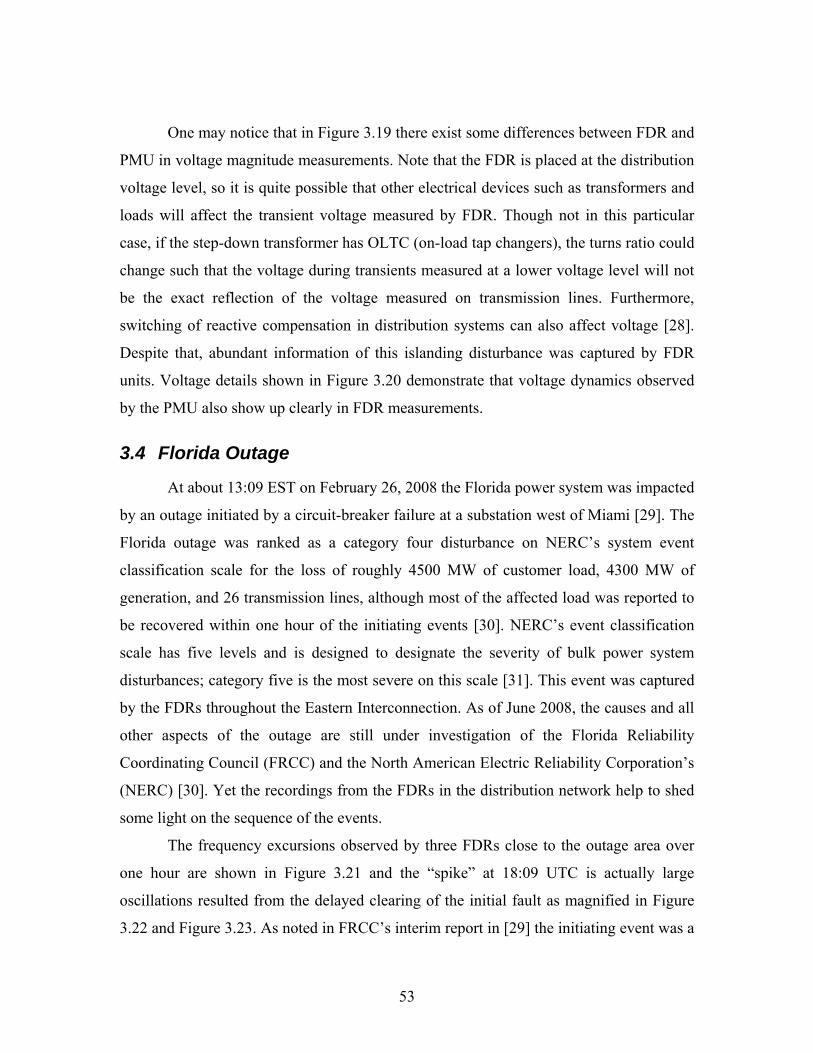
53
One may notice that in Figure 3.19 there exist some differences between FDR and
PMU in voltage magnitude measurements. Note that the FDR is placed at the distribution
voltage level, so it is quite possible that other electrical devices such as transformers and
loads will affect the transient voltage measured by FDR. Though not in this particular
case, if the step-down transformer has OLTC (on-load tap changers), the turns ratio could
change such that the voltage during transients measured at a lower voltage level will not
be the exact reflection of the voltage measured on transmission lines. Furthermore,
switching of reactive compensation in distribution systems can also affect voltage [28].
Despite that, abundant information of this islanding disturbance was captured by FDR
units. Voltage details shown in Figure 3.20 demonstrate that voltage dynamics observed
by the PMU also show up clearly in FDR measurements.
3.4 Florida Outage
At about 13:09 EST on February 26, 2008 the Florida power system was impacted
by an outage initiated by a circuit-breaker failure at a substation west of Miami [29]. The
Florida outage was ranked as a category four disturbance on NERC’s system event
classification scale for the loss of roughly 4500 MW of customer load, 4300 MW of
generation, and 26 transmission lines, although most of the affected load was reported to
be recovered within one hour of the initiating events [30]. NERC’s event classification
scale has five levels and is designed to designate the severity of bulk power system
disturbances; category five is the most severe on this scale [31]. This event was captured
by the FDRs throughout the Eastern Interconnection. As of June 2008, the causes and all
other aspects of the outage are still under investigation of the Florida Reliability
Coordinating Council (FRCC) and the North American Electric Reliability Corporation’s
(NERC) [30]. Yet the recordings from the FDRs in the distribution network help to shed
some light on the sequence of the events.
The frequency excursions observed by three FDRs close to the outage area over
one hour are shown in Figure 3.21 and the “spike” at 18:09 UTC is actually large
oscillations resulted from the delayed clearing of the initial fault as magnified in Figure
3.22 and Figure 3.23. As noted in FRCC’s interim report in [29] the initiating event was a
54
three-phase fault on a failed 138 kV switch at a transmission substation in south Florida.
The disabling of all local protective relay equipment while troubleshooting a transmission
switch led to delayed clearing of the fault which remained on the system for
approximately 1.7 seconds.
17:59:55 18:08:36 18:17:17 18:25:58 18:34:39 18:43:20 18:52:01 19:00:4259.85
59.9
59.95
60
60.05
60.1
60.15
60.2
Time (UTC)
Freq
uenc
y (H
z)
2008/2/26 10-point median
FDR42 - FSUFDR523 - TTU3FDR526 - SOCO
Figure 3.21 Frequency excursion between 18:00 to 19:00 UTC for the Florida outage
The depressed voltage (Figure 3.24) due to the fault led to protective trip of the
two Turkey Point generating units as well as some fossil generation in the region. The
FDR42 unit is in Florida therefore it clearly saw the voltage depression. The frequency
and angle swings radiated in the system as shown in Figure 3.23 and Figure 3.25 but the
frequency and angle perturbation was damped out within 10 seconds due to the isolation
of the fault and tripping of generators.
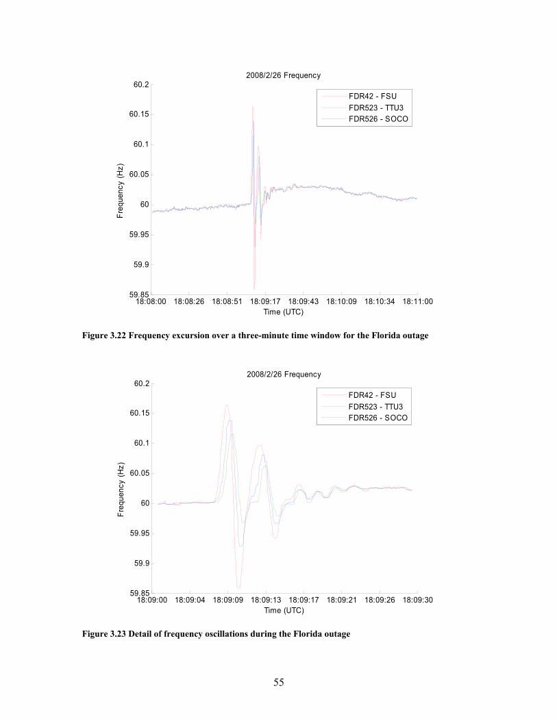
55
18:08:00 18:08:26 18:08:51 18:09:17 18:09:43 18:10:09 18:10:34 18:11:0059.85
59.9
59.95
60
60.05
60.1
60.15
60.2
Time (UTC)
Freq
uenc
y (H
z)
2008/2/26 Frequency
FDR42 - FSUFDR523 - TTU3FDR526 - SOCO
Figure 3.22 Frequency excursion over a three-minute time window for the Florida outage
18:09:00 18:09:04 18:09:09 18:09:13 18:09:17 18:09:21 18:09:26 18:09:3059.85
59.9
59.95
60
60.05
60.1
60.15
60.2
Time (UTC)
Freq
uenc
y (H
z)
2008/2/26 Frequency
FDR42 - FSUFDR523 - TTU3FDR526 - SOCO
Figure 3.23 Detail of frequency oscillations during the Florida outage
56
18:09:00 18:09:05 18:09:10 18:09:14 18:09:19 18:09:24 18:09:280.96
0.97
0.98
0.99
1
1.01
1.02
Time (UTC)
Vol
tage
(p.u
.)
2008/02/26 Voltage
FDR42 - FSUFDR523 - TTU3FDR526 - SOCO
Figure 3.24 Normalized voltage showing the voltage depression during the Florida outage
18:09:00 18:09:04 18:09:09 18:09:13 18:09:17 18:09:21 18:09:26 18:09:30-30
-20
-10
0
10
20
30
40
50
Time (UTC)
Ang
le (d
egre
e)
2008/2/26 Angle - FDR4 as reference
FDR42 - FSUFDR523 - TTU3FDR526 - SOCO
Figure 3.25 Detail of angle oscillations during the Florida outage (referred to FDR4)
57
The frequency increased immediately after the oscillations, which indicates
possible load loss but it started to decrease shortly. It is reported that the massive
generation loss drove the region to an under-frequency condition at about 59.95 Hz
between 18:10 to 18:16 UTC that led to under-frequency load shedding (Figure 3.21).
The Florida system was able to keep synchronized with the bulk EI system during the
frequency and voltage perturbations.
3.5 Faults in HVDC Systems
Three High-Voltage Direct-Current (HVDC) transmission related events observed
in the EI by FNET in 2008 are examined in this section. Two of them are the loss of the
Quebec – New England HVDC interconnection at different time, and the other is an
event at the Nelson River HVDC system. Both HVDC systems are bipolar transmission
and the configuration of a two-terminal bipolar link is depicted in Figure 3.26.
Transformer TransformerAC Bus
AC Bus
DC Line
DC Line
Figure 3.26 Configuration of bipolar HVDC link
A pair of conductors is used in opposite polarity. The system can operate with
only one pole in service (mono-polar mode) transferring half of the total rated capacity
58
when the other pole is out due to fault or maintenance. Each terminal has two converters
of equal rated voltage connected in series on the DC side. The junctions between the
converters are grounded. The valves in the converters are controlled electronic switches
that conduct in only in one direction.
3.5.1 Events in the Quebec – New England HVDC Interconnection on June 20 and October 25, 2008
As shown in Figure 3.27, the 920 mile long Quebec – New England HVDC line
connects the asynchronous Hydro Quebec system and the EI system with its north
terminal at Radisson, Canada and south terminal at Sandy Pond in Ayer, Massachusetts
[32]. The ± 450 kV multi-terminal HVDC lines can transmit about 2000 MW in either
direction [33].
Figure 3.27 Location of the Quebec – New England Phase II HVDC transmission line (map source:
USGS)
At 19:29:41 UTC on June 20, 2008 the frequency in the northeast EI experienced
large swings because of the disconnection of the Quebec – New England HVDC line due
to a failure of the protection and control system at Radisson. The loss of one pole also
59
resulted in a power loss of 500 MW which initiated a frequency decline of about 17 mHz
(Figure 3.28). It can be seen from the figure that the New England area was the power
receiving end that saw a loss of generation. The relative angle in the EI in Figure 3.29
reveals that the loss of the HVDC line accounted for an angle change and angle swings at
each of the three FDR locations. The initial decline in the angle also confirms that the
power was transmitted from Quebec to the EI system where the measurements were
taken. The angle signature is similar to that of the loss of an AC transmission line, which
will be discussed in detail in Chapter 5 and 6.
19:29:00 19:29:17 19:29:34 19:29:51 19:30:09 19:30:26 19:30:43 19:31:0059.965
59.97
59.975
59.98
59.985
59.99
59.995
60
60.005
60.01
60.015
Time (UTC)
Freq
uenc
y (H
z)
2008/6/20 Frequency
FDR539 - BangorFDR513 - PSUFDR516 - LeRoy
Figure 3.28 Frequency of the Quebec – New England HVDC event on June 20, 2008
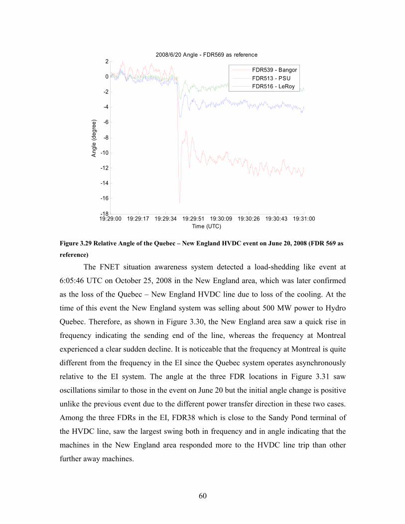
60
19:29:00 19:29:17 19:29:34 19:29:51 19:30:09 19:30:26 19:30:43 19:31:00-18
-16
-14
-12
-10
-8
-6
-4
-2
0
2
Time (UTC)
Ang
le (d
egre
e)
2008/6/20 Angle - FDR569 as reference
FDR539 - BangorFDR513 - PSUFDR516 - LeRoy
Figure 3.29 Relative Angle of the Quebec – New England HVDC event on June 20, 2008 (FDR 569 as
reference)
The FNET situation awareness system detected a load-shedding like event at
6:05:46 UTC on October 25, 2008 in the New England area, which was later confirmed
as the loss of the Quebec – New England HVDC line due to loss of the cooling. At the
time of this event the New England system was selling about 500 MW power to Hydro
Quebec. Therefore, as shown in Figure 3.30, the New England area saw a quick rise in
frequency indicating the sending end of the line, whereas the frequency at Montreal
experienced a clear sudden decline. It is noticeable that the frequency at Montreal is quite
different from the frequency in the EI since the Quebec system operates asynchronously
relative to the EI system. The angle at the three FDR locations in Figure 3.31 saw
oscillations similar to those in the event on June 20 but the initial angle change is positive
unlike the previous event due to the different power transfer direction in these two cases.
Among the three FDRs in the EI, FDR38 which is close to the Sandy Pond terminal of
the HVDC line, saw the largest swing both in frequency and in angle indicating that the
machines in the New England area responded more to the HVDC line trip than other
further away machines.
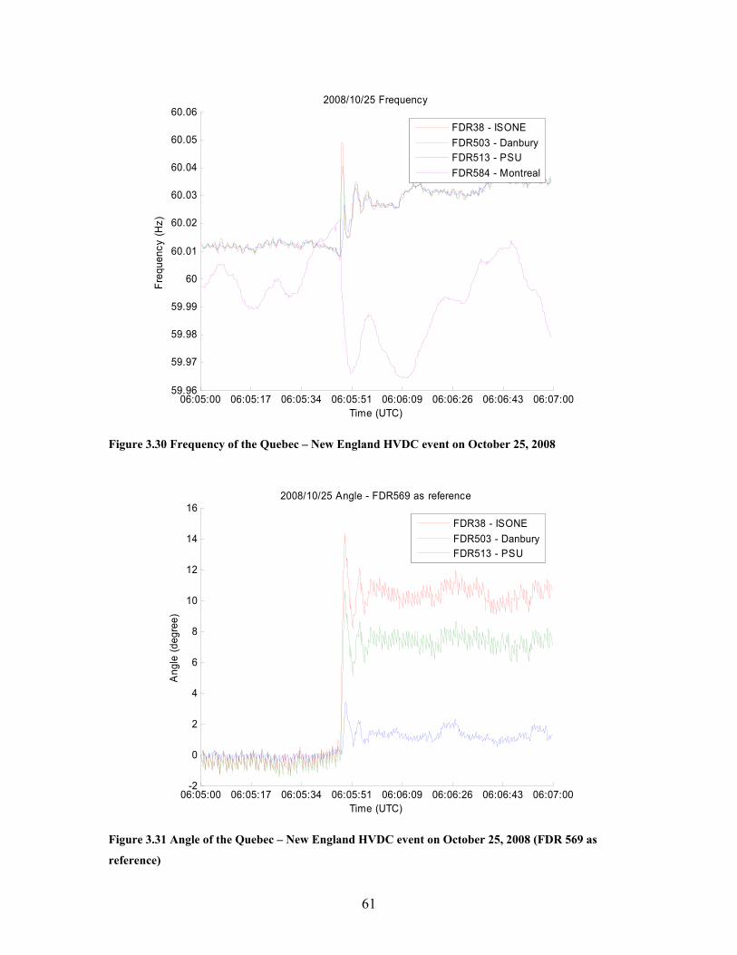
61
06:05:00 06:05:17 06:05:34 06:05:51 06:06:09 06:06:26 06:06:43 06:07:0059.96
59.97
59.98
59.99
60
60.01
60.02
60.03
60.04
60.05
60.06
Time (UTC)
Freq
uenc
y (H
z)
2008/10/25 Frequency
FDR38 - ISONEFDR503 - DanburyFDR513 - PSUFDR584 - Montreal
Figure 3.30 Frequency of the Quebec – New England HVDC event on October 25, 2008
06:05:00 06:05:17 06:05:34 06:05:51 06:06:09 06:06:26 06:06:43 06:07:00-2
0
2
4
6
8
10
12
14
16
Time (UTC)
Ang
le (d
egre
e)
2008/10/25 Angle - FDR569 as reference
FDR38 - ISONEFDR503 - DanburyFDR513 - PSU
Figure 3.31 Angle of the Quebec – New England HVDC event on October 25, 2008 (FDR 569 as
reference)
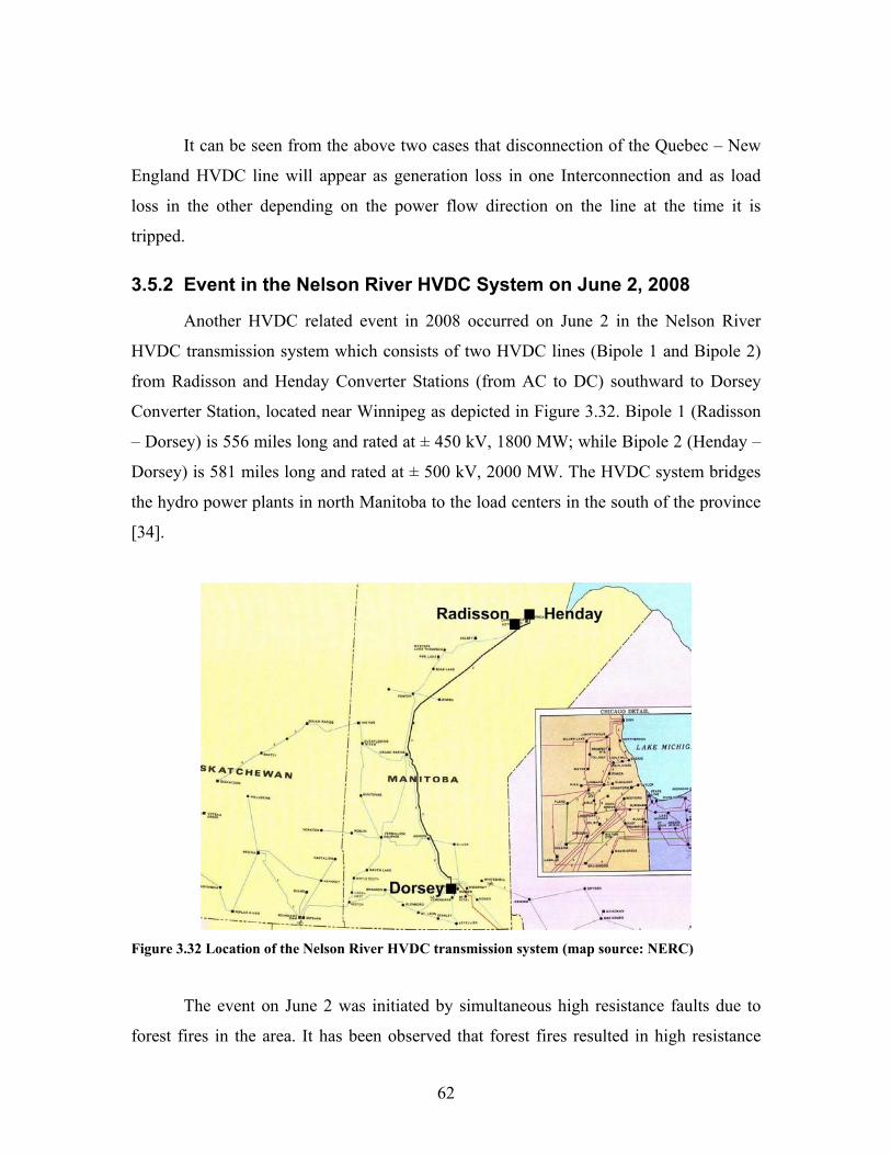
62
It can be seen from the above two cases that disconnection of the Quebec – New
England HVDC line will appear as generation loss in one Interconnection and as load
loss in the other depending on the power flow direction on the line at the time it is
tripped.
3.5.2 Event in the Nelson River HVDC System on June 2, 2008
Another HVDC related event in 2008 occurred on June 2 in the Nelson River
HVDC transmission system which consists of two HVDC lines (Bipole 1 and Bipole 2)
from Radisson and Henday Converter Stations (from AC to DC) southward to Dorsey
Converter Station, located near Winnipeg as depicted in Figure 3.32. Bipole 1 (Radisson
– Dorsey) is 556 miles long and rated at ± 450 kV, 1800 MW; while Bipole 2 (Henday –
Dorsey) is 581 miles long and rated at ± 500 kV, 2000 MW. The HVDC system bridges
the hydro power plants in north Manitoba to the load centers in the south of the province
[34].
Figure 3.32 Location of the Nelson River HVDC transmission system (map source: NERC)
The event on June 2 was initiated by simultaneous high resistance faults due to
forest fires in the area. It has been observed that forest fires resulted in high resistance
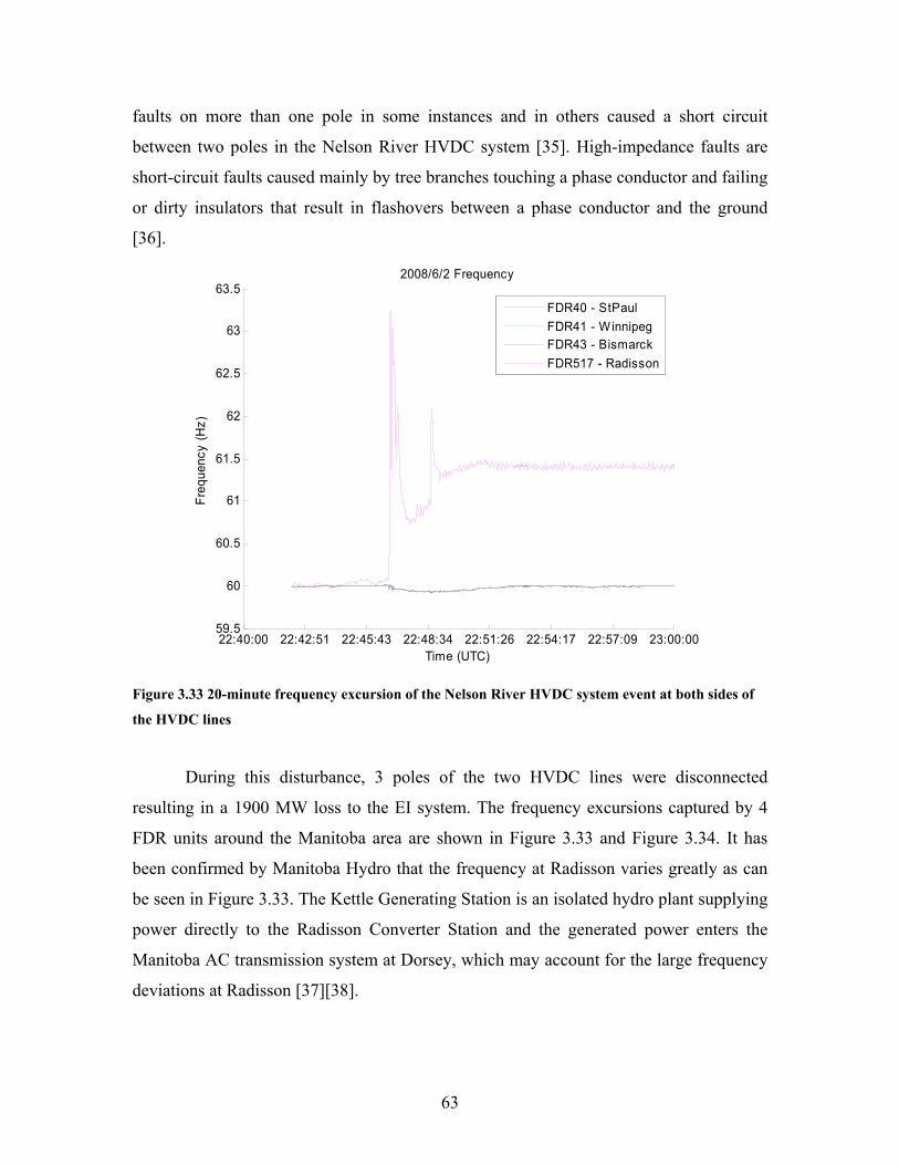
63
faults on more than one pole in some instances and in others caused a short circuit
between two poles in the Nelson River HVDC system [35]. High-impedance faults are
short-circuit faults caused mainly by tree branches touching a phase conductor and failing
or dirty insulators that result in flashovers between a phase conductor and the ground
[36].
22:40:00 22:42:51 22:45:43 22:48:34 22:51:26 22:54:17 22:57:09 23:00:0059.5
60
60.5
61
61.5
62
62.5
63
63.5
Time (UTC)
Freq
uenc
y (H
z)
2008/6/2 Frequency
FDR40 - StPaulFDR41 - WinnipegFDR43 - BismarckFDR517 - Radisson
Figure 3.33 20-minute frequency excursion of the Nelson River HVDC system event at both sides of
the HVDC lines
During this disturbance, 3 poles of the two HVDC lines were disconnected
resulting in a 1900 MW loss to the EI system. The frequency excursions captured by 4
FDR units around the Manitoba area are shown in Figure 3.33 and Figure 3.34. It has
been confirmed by Manitoba Hydro that the frequency at Radisson varies greatly as can
be seen in Figure 3.33. The Kettle Generating Station is an isolated hydro plant supplying
power directly to the Radisson Converter Station and the generated power enters the
Manitoba AC transmission system at Dorsey, which may account for the large frequency
deviations at Radisson [37][38].
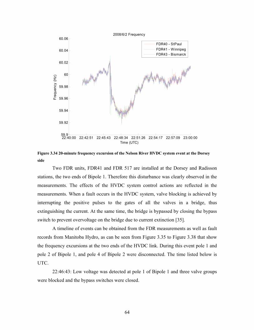
64
22:40:00 22:42:51 22:45:43 22:48:34 22:51:26 22:54:17 22:57:09 23:00:0059.9
59.92
59.94
59.96
59.98
60
60.02
60.04
60.06
Time (UTC)
Freq
uenc
y (H
z)
2008/6/2 Frequency
FDR40 - StPaulFDR41 - WinnipegFDR43 - Bismarck
Figure 3.34 20-minute frequency excursion of the Nelson River HVDC system event at the Dorsey
side
Two FDR units, FDR41 and FDR 517 are installed at the Dorsey and Radisson
stations, the two ends of Bipole 1. Therefore this disturbance was clearly observed in the
measurements. The effects of the HVDC system control actions are reflected in the
measurements. When a fault occurs in the HVDC system, valve blocking is achieved by
interrupting the positive pulses to the gates of all the valves in a bridge, thus
extinguishing the current. At the same time, the bridge is bypassed by closing the bypass
switch to prevent overvoltage on the bridge due to current extinction [35].
A timeline of events can be obtained from the FDR measurements as well as fault
records from Manitoba Hydro, as can be seen from Figure 3.35 to Figure 3.38 that show
the frequency excursions at the two ends of the HVDC link. During this event pole 1 and
pole 2 of Bipole 1, and pole 4 of Bipole 2 were disconnected. The time listed below is
UTC.
22:46:43: Low voltage was detected at pole 1 of Bipole 1 and three valve groups
were blocked and the bypass switches were closed.
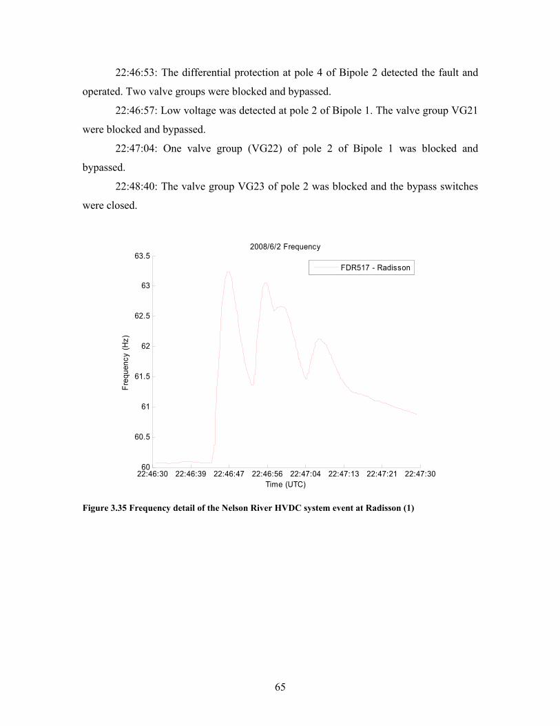
65
22:46:53: The differential protection at pole 4 of Bipole 2 detected the fault and
operated. Two valve groups were blocked and bypassed.
22:46:57: Low voltage was detected at pole 2 of Bipole 1. The valve group VG21
were blocked and bypassed.
22:47:04: One valve group (VG22) of pole 2 of Bipole 1 was blocked and
bypassed.
22:48:40: The valve group VG23 of pole 2 was blocked and the bypass switches
were closed.
22:46:30 22:46:39 22:46:47 22:46:56 22:47:04 22:47:13 22:47:21 22:47:3060
60.5
61
61.5
62
62.5
63
63.5
Time (UTC)
Freq
uenc
y (H
z)
2008/6/2 Frequency
FDR517 - Radisson
Figure 3.35 Frequency detail of the Nelson River HVDC system event at Radisson (1)
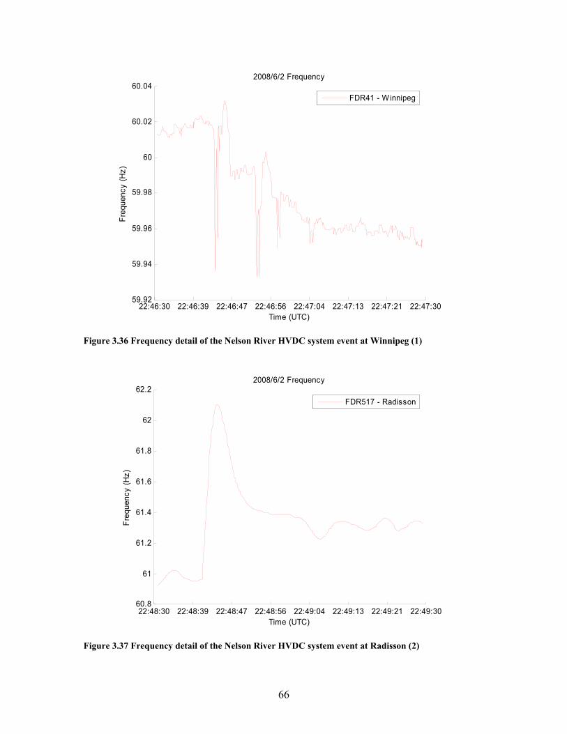
66
22:46:30 22:46:39 22:46:47 22:46:56 22:47:04 22:47:13 22:47:21 22:47:3059.92
59.94
59.96
59.98
60
60.02
60.04
Time (UTC)
Freq
uenc
y (H
z)
2008/6/2 Frequency
FDR41 - Winnipeg
Figure 3.36 Frequency detail of the Nelson River HVDC system event at Winnipeg (1)
22:48:30 22:48:39 22:48:47 22:48:56 22:49:04 22:49:13 22:49:21 22:49:3060.8
61
61.2
61.4
61.6
61.8
62
62.2
Time (UTC)
Freq
uenc
y (H
z)
2008/6/2 Frequency
FDR517 - Radisson
Figure 3.37 Frequency detail of the Nelson River HVDC system event at Radisson (2)
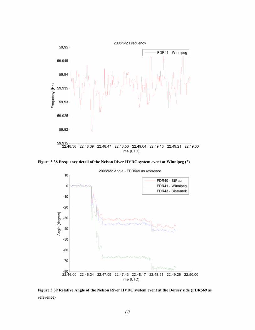
67
22:48:30 22:48:39 22:48:47 22:48:56 22:49:04 22:49:13 22:49:21 22:49:3059.915
59.92
59.925
59.93
59.935
59.94
59.945
59.95
Time (UTC)
Freq
uenc
y (H
z)
2008/6/2 Frequency
FDR41 - Winnipeg
Figure 3.38 Frequency detail of the Nelson River HVDC system event at Winnipeg (2)
22:46:00 22:46:34 22:47:09 22:47:43 22:48:17 22:48:51 22:49:26 22:50:00-80
-70
-60
-50
-40
-30
-20
-10
0
10
Time (UTC)
Ang
le (d
egre
e)
2008/6/2 Angle - FDR569 as reference
FDR40 - StPaulFDR41 - WinnipegFDR43 - Bismarck
Figure 3.39 Relative Angle of the Nelson River HVDC system event at the Dorsey side (FDR569 as
reference)

68
From the timeline and the figures one can tell that each time when a pole loss
occurs frequency oscillations can be observed but the frequency change was opposite at
the two ends of the HVDC connection. The angle observed at the Dorsey side of the
HVDC line demonstrates a step change of angle decline at each pole loss and valve group
blocking, together with angle swings, while FDR41 at the Dorsey station saw the largest
angle change (Figure 3.39).
3.6 Dynamic Performance of AD/DC Systems
As mentioned in section 3.5, the hydro power plants at the north terminal of the
Nelson River HVDC system are isolated with no AC loads, thus the generators have no
benefit of the load damping. Moreover, the neighboring AC systems Manitoba Hydro is
interconnected with are relatively weak in the area. The HVDC links, when controlled in
the constant power mode, appear to be frequency insensitive loads to the AC systems and
may provide negative damping to system swings. DC links do not inherently allow the
flow of synchronizing power in response to a disturbance. Due to this system
characteristic, special auxiliary power controls have been studied and implemented to
improve the dynamic performance of the interconnected AC/DC systems as described in
references [27] and [38].
With the installation of the FDRs at the two terminals (Radisson and Dorsey) of
the Nelson River HVDC Bipole 1, they dynamic performance of the AC/DC systems and
the effects of the damping controls are able to be observed in the time-synchronized
measurements. Each bipole in the Nelson River HVDC system has frequency control at
both the sending end and the receiving end. The sending-end frequency control provides
power order modulation according to the frequency deviation at the Radisson and Henday
stations, thus making the DC link load frequency sensitive. Without such control the
generators feeding the DC load are subject to a torque which varies inversely with the
frequency since
ωTP = (3.1)
where T is the torque in mN ⋅ and ω is the angle velocity in rad/s.
69
The receiving-end frequency control is provided to minimize the frequency
deviation in the system. In addition, the damping controls also include receiving-end
phase angle control that helps to maintain the stability of the south Manitoba system
during disturbances.
In this section three disturbances near south Manitoba detected by the FNET are
investigated to illustrate the effects of the damping controls in the HVDC system. The
frequency is observed on both ends of the HVDC links. Figure 3.40 and Figure 3.41 show
the frequency of a generation loss event detected on June 24, 2008 and a load loss event
on November 2, 2008, respectively.
21:04:30 21:04:47 21:05:04 21:05:21 21:05:39 21:05:56 21:06:13 21:06:3059.98
59.99
60
60.01
60.02
60.03
60.04
60.05
60.06
60.07
60.08
60.09
60.1
60.11
60.12
60.13
Time (UTC)
Freq
uenc
y (H
z)
2008/6/24 Frequency
FDR41 - WinnipegFDR517 - Radisson
Figure 3.40 Frequency observed at both sides of the HVDC line during a generation loss event in the
EI on June 24, 2008
As can be seen from Figure 3.40, the fast frequency decline and swings at
Winnipeg due to the disturbance are clearly observed at Radisson. The frequency
deviation during the disturbance is different at the two ends of the HVDC line because of
different frequency response characteristics due to different amount of inertia.
70
10:29:00 10:29:17 10:29:34 10:29:51 10:30:09 10:30:26 10:30:43 10:31:0060.01
60.02
60.03
60.04
60.05
60.06
60.07
60.08
60.09
60.1
60.11
60.12
60.13
60.14
Time (UTC)
Freq
uenc
y (H
z)
2008/11/2 Frequency
FDR43 - BismarckFDR517 - Radisson
Figure 3.41 Frequency observed at both sides of the HVDC line during a load loss event in the EI on
November 2, 2008
10:01:30 10:01:47 10:02:04 10:02:21 10:02:39 10:02:56 10:03:13 10:03:3059.9559.9659.9759.9859.99
6060.0160.0260.0360.0460.0560.0660.0760.0860.09
60.160.1160.1260.1360.1460.1560.1660.1760.1860.19
Time (UTC)
Freq
uenc
y (H
z)
2008/5/19 Frequency
FDR41 - WinnipegFDR517 - Radisson
Figure 3.42 Frequency observed at both sides of the HVDC line during a load loss event in the EI on
May 19, 2008

71
Such correlation is not obvious during steady state since the damping controls
described above are designed to respond to fast transients caused by disturbances and not
steady-state variations [38]. The instance in Figure 3.41 agrees with this concept in that
the sharp frequency rise at the Dorsey end of the system is also ‘translated’ to the other
end of the DC link.
Figure 3.42 shows a load loss event in the EI system south to the HVDC system
but not observed by the FDR at Radisson. The frequency at Winnipeg and Radisson does
not show much similarity perhaps because the frequency transient resulted from the load
loss is not large enough or too gradual to be reflected across the DC link.
In summary, for large fast changes in frequency we can expect to see the
continuation of the frequency excursion temporarily across the DC link given the DC link
has damping controls. For gradual frequency changes we can expect no frequency
information on the other side of the DC interconnections. By monitoring the DC links
with damping controls, the impact of the HVDC transmission system on the overall
dynamic performance of the AC/DC systems can be studied, which may benefit the study
of disturbance location and system inertia calculation. Furthermore, the wide-area
measurements from PMU and FNET can provide system-wide information to assist
designing the HVDC damping controllers to enhance the dynamic performance of the
interconnected power systems [39].
While the damping controls in the Nelson River HVDC system adjust the power
flow on the DC links as the frequency in the AC systems changes, controls in other
HVDC systems may not be frequency sensitive in order to prevent the disturbances in
one area from propagating to the other. The North America bulk power systems consist
of four main asynchronous Interconnections: the EI, the WECC, the ERCOT and the
Quebec. They are interconnected by HVDC ties that can buffer one AC system from
disturbances in the other. Three events detected in the EI shown in Figure 3.43 to Figure
3.45 confirm that the disturbances in one Interconnection will not be detected in others
that do not operate synchronously.
72
19:07:00 19:07:17 19:07:34 19:07:51 19:08:09 19:08:26 19:08:43 19:09:0059.94
59.95
59.96
59.97
59.98
59.99
60
60.01
60.02
60.03
60.04
Time (UTC)
Freq
uenc
y (H
z)
2008/10/24 Frequency
FDR38 - ISONEFDR584 - Montreal
Figure 3.43 Frequency in the EI and Quebec during a generator trip event in the EI
10:29:00 10:29:17 10:29:34 10:29:51 10:30:09 10:30:26 10:30:43 10:31:0059.98
59.99
60
60.01
60.02
60.03
60.04
60.05
Time (UTC)
Freq
uenc
y (H
z)
2008/11/2 Frequency
FDR43 - Bismarck FDR572 - WSU
Figure 3.44 Frequency in the EI and the WECC during a load loss event in the EI
73
04:21:30 04:21:47 04:22:04 04:22:21 04:22:39 04:22:56 04:23:13 04:23:3059.94
59.95
59.96
59.97
59.98
59.99
60
60.01
60.02
60.03
60.04
60.05
60.06
Time (UTC)
Freq
uenc
y (H
z)
2008/11/4 Frequency
FDR551 - TXFDR566 - Gulfport
Figure 3.45 Frequency in the EI and the ERCOT during a generator trip event in the EI
Further, the HVDC controls may vary for different control needs and various AC
system conditions [21][27]. In the case of the Quebec – New England HVDC system, the
power network at the south end of the HVDC link is very strong thus no need for
frequency dependent HVDC power modulation. The power generating station La Grande
2A at the north Radisson end is usually isolated from the Quebec system and feeds the
HVDC link directly. Therefore, HVDC power is modulated to maintain the frequency in
the collector system within the range between 59.5 Hz and 61.5 Hz. The effect of the DC
power flow modulation is expected to be observed if a sensor is installed at the Radisson
station in Quebec.
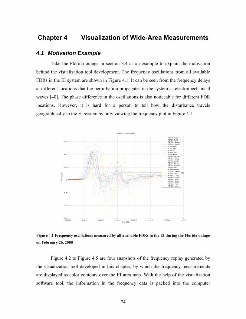
74
Chapter 4 Visualization of Wide-Area Measurements
4.1 Motivation Example
Take the Florida outage in section 3.4 as an example to explain the motivation
behind the visualization tool development. The frequency oscillations from all available
FDRs in the EI system are shown in Figure 4.1. It can be seen from the frequency delays
at different locations that the perturbation propagates in the system as electromechanical
waves [40]. The phase difference in the oscillations is also noticeable for different FDR
locations. However, it is hard for a person to tell how the disturbance travels
geographically in the EI system by only viewing the frequency plot in Figure 4.1.
Figure 4.1 Frequency oscillations measured by all available FDRs in the EI during the Florida outage
on February 26, 2008
Figure 4.2 to Figure 4.5 are four snapshots of the frequency replay generated by
the visualization tool developed in this chapter, by which the frequency measurements
are displayed as color contours over the EI area map. With the help of the visualization
software tool, the information in the frequency data is packed into the computer
18:09:06 18:09:09 18:09:11 18:09:14 18:09:17 18:09:19 18:09:22 18:09:2559.85
59.9
59.95
60
60.05
60.1
60.15
Time (UTC)
Freq
uenc
y (H
z)
2008/2/26 10-point median
FDR13 - MISOFDR20 - TVA2FDR500 - ChicagoFDR508 - RVCSFDR2 - UMRFDR3 - ARIFDR4 - VTFDR35 - ISUFDR7 - MISSIFDR11 - CALVINFDR510 - BburgFDR38 - ISONEFDR40 - StPaulFDR41 - WinnipegFDR42 - FSUFDR43 - BismarckFDR503 - DanburyFDR513 - PSUFDR516 - LeRoyFDR521 - ChillicoFDR523 - TTU3FDR526 - SOCOFDR535 - PJMFDR554 - Loui
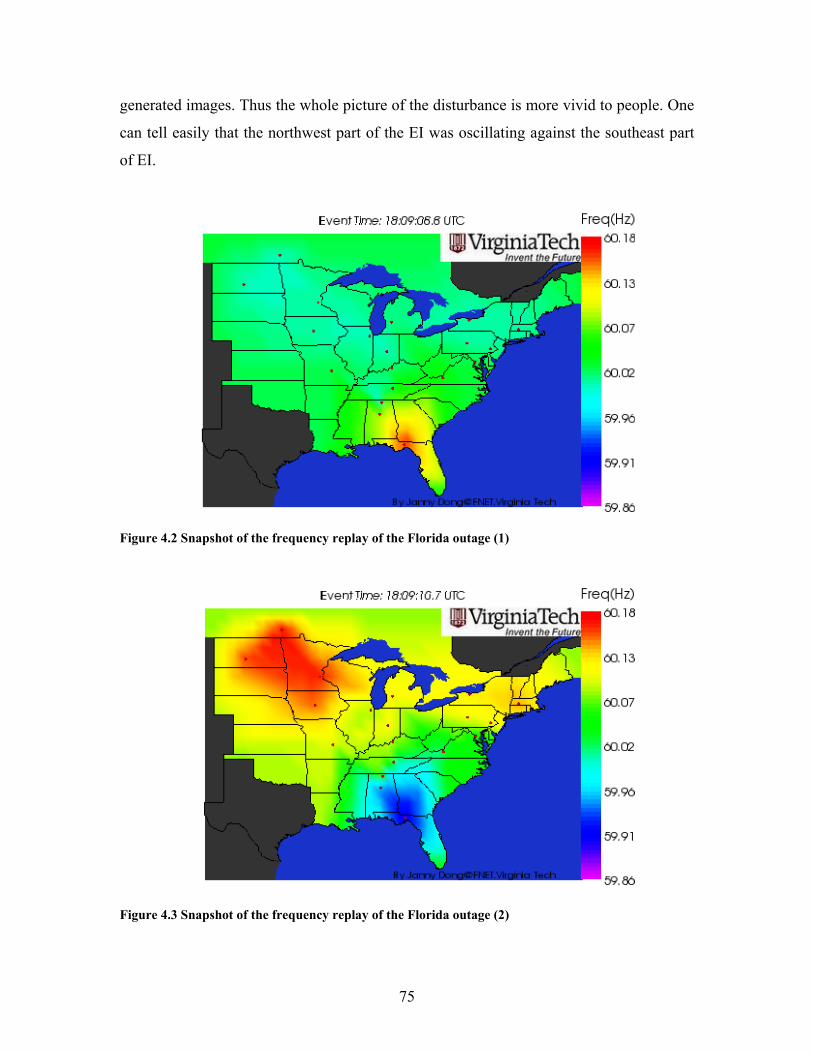
75
generated images. Thus the whole picture of the disturbance is more vivid to people. One
can tell easily that the northwest part of the EI was oscillating against the southeast part
of EI.
Figure 4.2 Snapshot of the frequency replay of the Florida outage (1)
Figure 4.3 Snapshot of the frequency replay of the Florida outage (2)
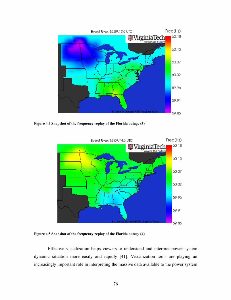
76
Figure 4.4 Snapshot of the frequency replay of the Florida outage (3)
Figure 4.5 Snapshot of the frequency replay of the Florida outage (4)
Effective visualization helps viewers to understand and interpret power system
dynamic situation more easily and rapidly [41]. Visualization tools are playing an
increasingly important role in interpreting the massive data available to the power system
77
engineers and improve situation awareness [42]. Various applications have been studied
and developed for visualizing power system states such as voltage [43] and load flow
[44]; as well as for educational purpose [45][46]. There also exist a variety of
visualization types: diagrams, pie charts, color contours and animations, etc. [47].
In order to better observe and understand the system dynamics during
disturbances, a visualization tool is developed in this chapter that correlates the wide-area
measurements with their geographical information by displaying the measurements as 2-
D colored surfaces over the EI map.
4.2 Visualization Tool Overview
The visualization tool developed in this chapter collects frequency and angle
measurements to form color contours over a geographical area, thus the generated
disturbance replay provides insights to electromechanical wave propagation in major
events. The saved frequency data of the Interconnection, combined with geographic and
system topology information, will be mapped to colors and displayed as color contours
which are obtained by a linear fit through all the active measuring points in each major
disturbance. The visualization is realized by using objects provided by the Visualization
Toolkit (VTK), which is an open-source, object-oriented software system for computer
graphics, visualization, and image processing [48]. C++ is chosen as the programming
language because the tool is expected to be implemented online as one function module
of the present FNET situation awareness system which is developed with C++.
4.2.1 The Visualization Toolkit
The Visualization ToolKit (VTK) is an open source, freely available software
system for 3D computer graphics, image processing, and visualization. VTK includes a
textbook published by Kitware [49], a C++ class library, and several interpreted interface
layers including Tcl/Tk, Java, and Python. The design and implementation of the library
has been strongly influenced by object-oriented principles.
The graphics model in VTK is at a higher level of abstraction than rendering
libraries like OpenGL or PEX. This means it is much easier to create useful graphics and
visualization applications. In VTK applications can be written directly in C++, Tcl, Java,

78
or Python. In this work, objects provided by VTK are used to map frequency
measurements to colors to generate frequency contours, and write image frames to form
AVI movies.
4.2.2 MATCOM Math Library
MATCOM is a Matlab to C++ complier developed by MathTools Ltd. which
enables easy integration of m-files code and algorithms into existing C++ projects.
MATCOM creates MEX files, DLL files for Excel and Visual Basic and standalone C++
applications, with royalty free distribution. MATCOM includes the supporting
Matrix<LIB> C++ matrix library that allows employing functions built in MATLAB in
C++ projects, which saves development time. The library is supplied as a group of DLLs
for Windows, resulting in very small executables.
Matrix<LIB> is a scientific C++ library which provides a double-precision matrix
type, Mm, that may be complex, real, sparse or n-dimensional. Over 600 functions and
overloaded operators are available. Included are basic operators, such as + - / * and
flexible indexing operations. Functions are provided for linear algebra, polynomial
arithmetic, signal processing, file I/O and more. The functions supplied were carefully
optimized for best matrix performance [50]. The Matrix<LIB> library is employed to
interpolate the measurements to be visualized to form a two dimension data mesh for the
color surface.
4.3 Design of the Visualization Tool
The procedures to generate measurement playbacks are shown in Figure 4.6. The
program can be divided to four main parts: obtain information about FDR locations and
measurement data, form interpolation matrix, map measurement values to colors and
conceal irrelevant areas, and write image frames into an AVI file.
79
Figure 4.6 Flowchart of the automated replay tool
When an event occurs in power systems, the event detection program in the FNET
situation awareness system will detect it and measurement data within a pre-determined
time frame (both before and after event) will be saved. The saved frequency data of the
Interconnection, combined with geographic and system topology information, will be
mapped to colors and displayed as color contours by using objects provided by the
Visualization Toolkit (VTK). A map of the Eastern Interconnection is divided into mesh
grids, each with a frequency value, which is obtained by a linear fit through all the active
measuring points in each major disturbance. Finally, the color contour map of each time
step will be lined up along the time axis to create the animation. It could provide
operators a prompt analysis of system operation situation and eventually help them to
take appropriate steps to prevent future system deterioration.
80
4.3.1 Read Measurements
The design objective of the visualization tool is to develop a stand-alone program
as well as an application module that can be easily integrated into the FNET situation
awareness system. The current disturbance detection program captures a generation loss
or a load shedding event then saves 40 seconds worth of data around the event time.
Taking into account of the FNET server structure, the visualization tool takes the event
data saved by the disturbance detection program as input. The procedure of reading data
is illustrated in Figure 4.7.
Figure 4.7 Procedures to read data
1) Read Unit Information
The FDR information is obtained from the "UnitConfig.txt" file as shown in
Figure 4.8. This unit configuration file contains the name and location information in
latitudes and longitudes that is necessary for the map display.
The FDR information is stored and managed in the vectors of the C++ Standard
Template Library (STL). The vector data structure allows quick and easy memory
allocation for specific data storage without explicit memory management. This makes
them particularly useful for storing data in lists whose length may not be known prior to
setting up the variable [51]. The management of the FDR information in vectors is
illustrated in Figure 4.9, where N is the total number of units in the EI, for example.
81
Figure 4.8 An example of UnitConfig.txt
Figure 4.9 Illustration of managing the FDR information with the vector structure
2) Read Event Information
The event information such as the event time and the estimated location is saved
in the file "EventLocation.txt" as shown in Figure 4.10, which is automatically created by
the location estimation module of the server program once a disturbance is detected.
82
Figure 4.10 An example of EventLocation.txt
3) Data Conditioning
The FNET server is designed to receive data from each FDR and save it. Each
FDR sends a packet of measurements 10 times each second. The packet consists of such
data as the GPS date, GPS time, frequency, phase angle, and voltage magnitude.
Comparisons and studies have confirmed that the time stamp of a FDR output is 11
seconds ahead of the PMU measurements for the same time period. The timing buffer
design of the FDR hardware accounts for this delay as elaborated with details in [52].
However, the delay may be occasionally 10 seconds for some devices when the buffers
are not filled due to loss of GPS messages. It is critical to correct such delays between
FDR units to achieve valid analysis results.
Figure 4.11 shows the format of the event data file automatically created for a
captured disturbance. The third column in the data file indicated the time delay of a
certain unit and normally it is around 11 seconds. The one-second delay problem between
FDR units is fixed by searching the units with incorrect time delay and subtracting one
second from their time stamps. After the measurements are correctly aligned, they are fed
into a 9-point moving median filter to remove the high-frequency noises.
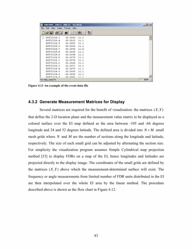
83
Figure 4.11 An example of the event data file
4.3.2 Generate Measurement Matrices for Display
Several matrices are required for the benefit of visualization: the matrices ),( YX
that define the 2-D location plane and the measurement value matrix to be displayed as a
colored surface over the EI map defined as the area between -105 and -66 degrees
longitude and 24 and 52 degrees latitude. The defined area is divided into MN × small
mesh grids where N and M are the number of sections along the longitude and latitude,
respectively. The size of each small grid can be adjusted by alternating the section size.
For simplicity the visualization program assumes Simple Cylindrical map projection
method [53] to display FDRs on a map of the EI, hence longitudes and latitudes are
projected directly to the display image. The coordinates of the small grids are defined by
the matrices ),( YX above which the measurement-determined surface will exist. The
frequency or angle measurements from limited number of FDR units distributed in the EI
are then interpolated over the whole EI area by the linear method. The procedure
described above is shown as the flow chart in Figure 4.12.
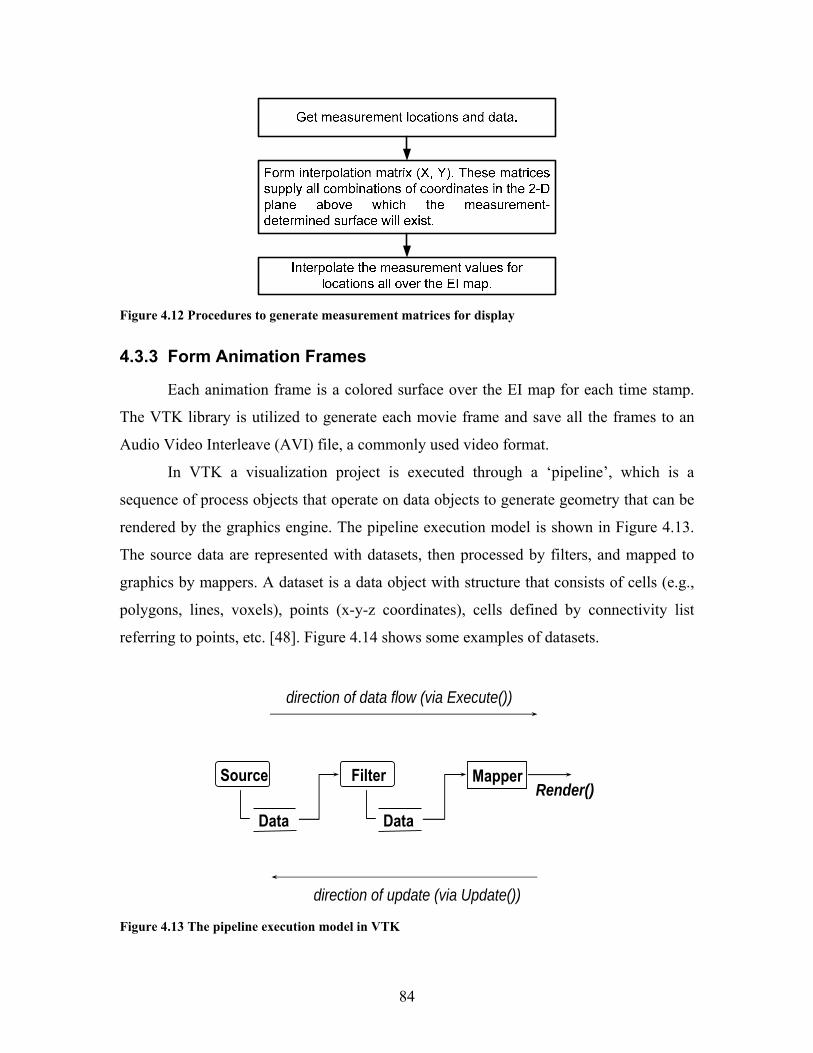
84
Figure 4.12 Procedures to generate measurement matrices for display
4.3.3 Form Animation Frames
Each animation frame is a colored surface over the EI map for each time stamp.
The VTK library is utilized to generate each movie frame and save all the frames to an
Audio Video Interleave (AVI) file, a commonly used video format.
In VTK a visualization project is executed through a ‘pipeline’, which is a
sequence of process objects that operate on data objects to generate geometry that can be
rendered by the graphics engine. The pipeline execution model is shown in Figure 4.13.
The source data are represented with datasets, then processed by filters, and mapped to
graphics by mappers. A dataset is a data object with structure that consists of cells (e.g.,
polygons, lines, voxels), points (x-y-z coordinates), cells defined by connectivity list
referring to points, etc. [48]. Figure 4.14 shows some examples of datasets.
direction of update (via Update())
Source
Data
Filter
Data
MapperRender()
direction of data flow (via Execute())
Figure 4.13 The pipeline execution model in VTK

85
vtkPolyDatavtkStructuredPoints
vtkStructuredGridvtkUnstructuredGrid
vtkRectilinearGrid
Figure 4.14 Dataset types in VTK
For example, the visualization program developed in this chapter uses an instance
of vtkPolyData to represent measurements. The coordinates of each measurement are
represented by points, and the corresponding frequency or angle values are represented
by scalars. Then vtkLookupTable maps the frequency scalars to colors. Finally vtkActor
represents all the geometries (lines, points, etc.) in a render window and a movie frame is
thus created. The detailed procedure can be found in Figure 4.15. More information about
the development of the visualization tool and the C++ code are listed in Appendix II.
Some graphic models and their functionalities are
• RenderWindow - contains final image
• Renderer - draws into render window
• Actor - combines properties / geometry
• Mappers - represent geometry
• Transformations - position actors
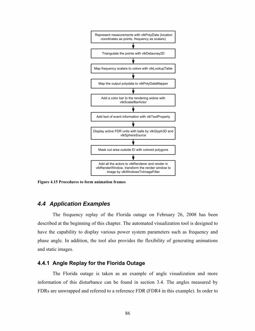
86
Represent measurements with vtkPolyData (location coordinates as points, frequency as scalars)
Triangulate the points with vtkDelaunay2D
Map frequency scalars to colors with vtkLookupTable
Map the output polydata to vtkPolyDataMapper
Add a color bar to the rendering widow with vtkScalarBarActor
Add text of event information with vtkTextProperty
Display active FDR units with balls by vtkGlyph3D and vtkSphereSource
Mask out area outside EI with colored polygons
Add all the actors to vtkRenderer and render in vtkRenderWindow, transform the render window to
image by vtkWindowsToImageFilter
Figure 4.15 Procedures to form animation frames
4.4 Application Examples
The frequency replay of the Florida outage on February 26, 2008 has been
described at the beginning of this chapter. The automated visualization tool is designed to
have the capability to display various power system parameters such as frequency and
phase angle. In addition, the tool also provides the flexibility of generating animations
and static images.
4.4.1 Angle Replay for the Florida Outage
The Florida outage is taken as an example of angle visualization and more
information of this disturbance can be found in section 3.4. The angles measured by
FDRs are unwrapped and referred to a reference FDR (FDR4 in this example). In order to
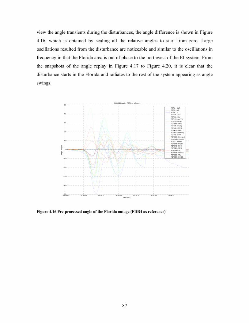
87
view the angle transients during the disturbances, the angle difference is shown in Figure
4.16, which is obtained by scaling all the relative angles to start from zero. Large
oscillations resulted from the disturbance are noticeable and similar to the oscillations in
frequency in that the Florida area is out of phase to the northwest of the EI system. From
the snapshots of the angle replay in Figure 4.17 to Figure 4.20, it is clear that the
disturbance starts in the Florida and radiates to the rest of the system appearing as angle
swings.
18:09:05 18:09:08 18:09:11 18:09:14 18:09:16 18:09:19 18:09:22-50
-40
-30
-20
-10
0
10
20
30
40
50
Time (UTC)
Ang
le (d
egre
e)
2008/2/26 Angle - FDR4 as reference
FDR2 - UMRFDR3 - ARIFDR4 - VTFDR20 - TVA2FDR35 - ISUFDR11 - CALVINFDR13 - MISOFDR510 - ROAFDR38 - BburgFDR40 - ISONEFDR41 - StPaulFDR42 - WinnipegFDR43 - FSUFDR500 - BismarckFDR503 - TorontoFDR7 - WayneFDR513 - MISSIFDR516 - PSUFDR521 - NPNFDR523 - SCFDR526 - ChillicoFDR535 - TTUFDR554 - SOCO
Figure 4.16 Pre-processed angle of the Florida outage (FDR4 as reference)
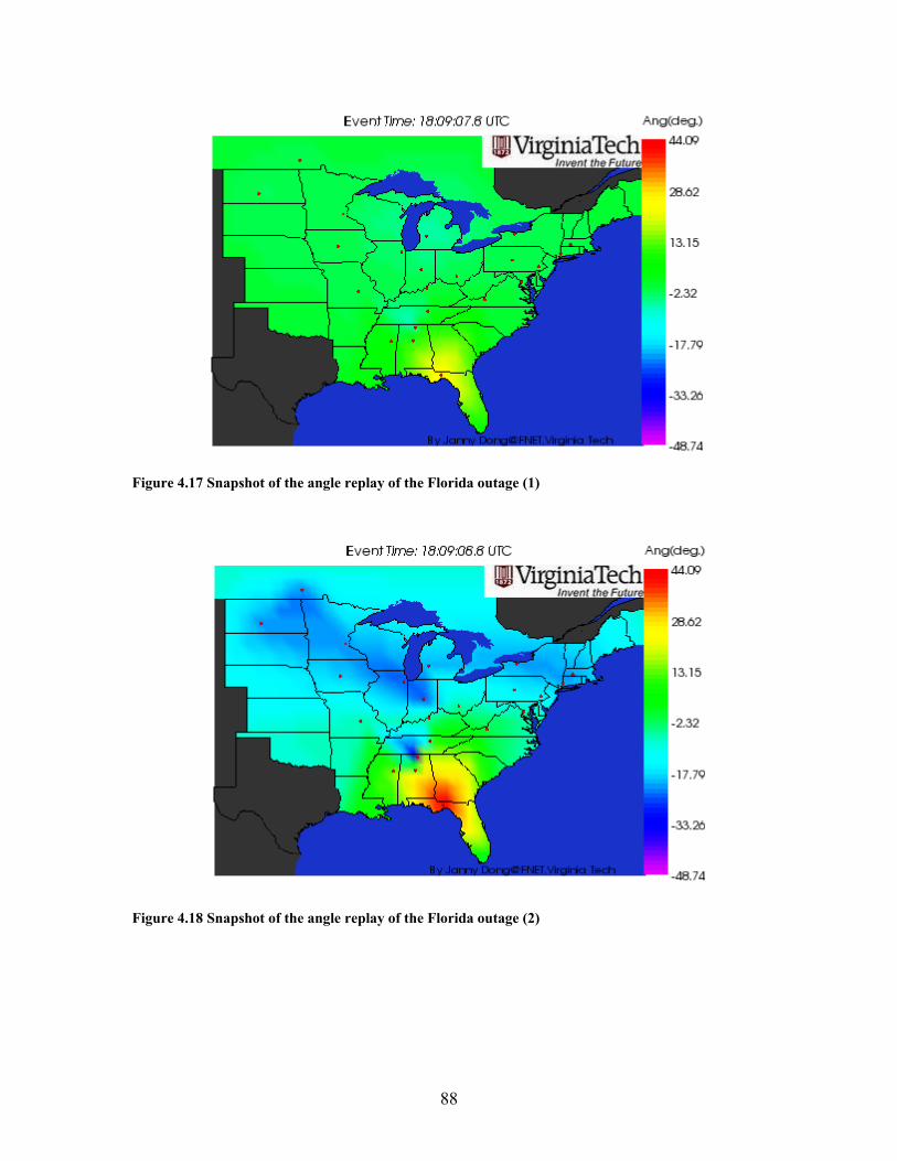
88
Figure 4.17 Snapshot of the angle replay of the Florida outage (1)
Figure 4.18 Snapshot of the angle replay of the Florida outage (2)
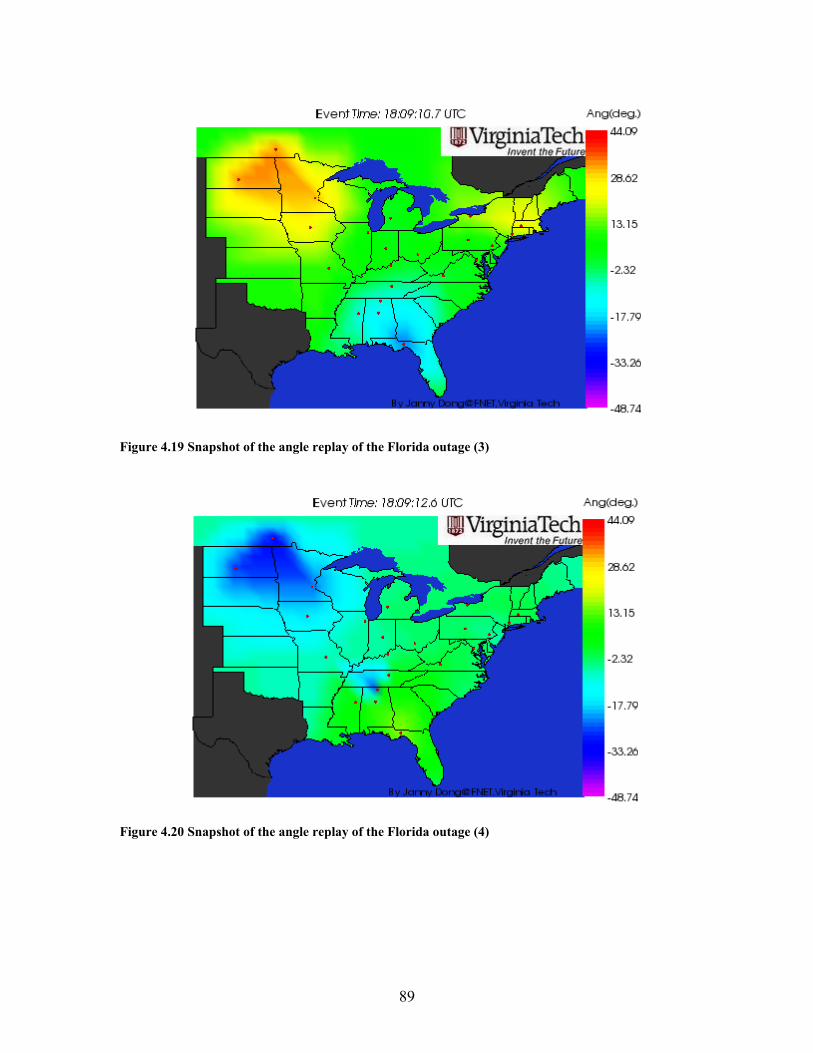
89
Figure 4.19 Snapshot of the angle replay of the Florida outage (3)
Figure 4.20 Snapshot of the angle replay of the Florida outage (4)
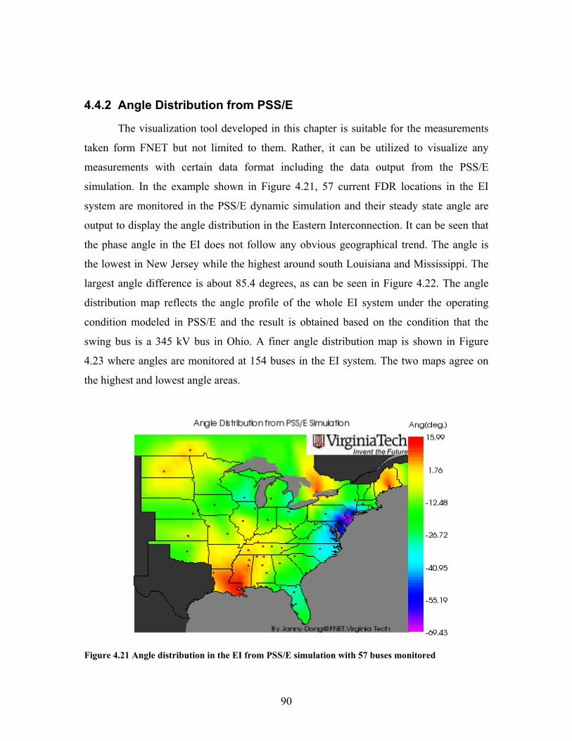
90
4.4.2 Angle Distribution from PSS/E
The visualization tool developed in this chapter is suitable for the measurements
taken form FNET but not limited to them. Rather, it can be utilized to visualize any
measurements with certain data format including the data output from the PSS/E
simulation. In the example shown in Figure 4.21, 57 current FDR locations in the EI
system are monitored in the PSS/E dynamic simulation and their steady state angle are
output to display the angle distribution in the Eastern Interconnection. It can be seen that
the phase angle in the EI does not follow any obvious geographical trend. The angle is
the lowest in New Jersey while the highest around south Louisiana and Mississippi. The
largest angle difference is about 85.4 degrees, as can be seen in Figure 4.22. The angle
distribution map reflects the angle profile of the whole EI system under the operating
condition modeled in PSS/E and the result is obtained based on the condition that the
swing bus is a 345 kV bus in Ohio. A finer angle distribution map is shown in Figure
4.23 where angles are monitored at 154 buses in the EI system. The two maps agree on
the highest and lowest angle areas.
Figure 4.21 Angle distribution in the EI from PSS/E simulation with 57 buses monitored
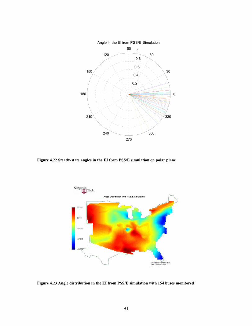
91
0.2
0.4
0.6
0.8
1
30
210
60
240
90
270
120
300
150
330
180 0
Angle in the EI from PSS/E Simulation
Figure 4.22 Steady-state angles in the EI from PSS/E simulation on polar plane
Figure 4.23 Angle distribution in the EI from PSS/E simulation with 154 buses monitored
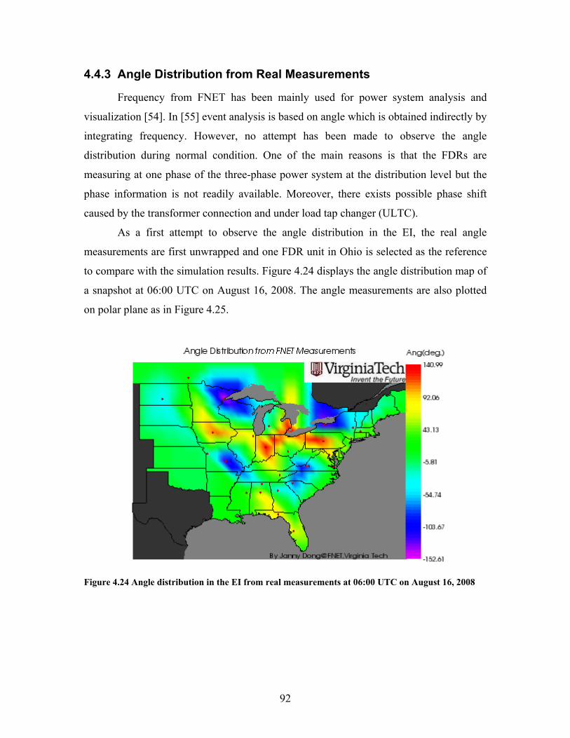
92
4.4.3 Angle Distribution from Real Measurements
Frequency from FNET has been mainly used for power system analysis and
visualization [54]. In [55] event analysis is based on angle which is obtained indirectly by
integrating frequency. However, no attempt has been made to observe the angle
distribution during normal condition. One of the main reasons is that the FDRs are
measuring at one phase of the three-phase power system at the distribution level but the
phase information is not readily available. Moreover, there exists possible phase shift
caused by the transformer connection and under load tap changer (ULTC).
As a first attempt to observe the angle distribution in the EI, the real angle
measurements are first unwrapped and one FDR unit in Ohio is selected as the reference
to compare with the simulation results. Figure 4.24 displays the angle distribution map of
a snapshot at 06:00 UTC on August 16, 2008. The angle measurements are also plotted
on polar plane as in Figure 4.25.
Figure 4.24 Angle distribution in the EI from real measurements at 06:00 UTC on August 16, 2008
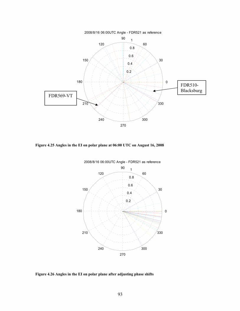
93
0.2
0.4
0.6
0.8
1
30
210
60
240
90
270
120
300
150
330
180 0
2008/8/16 06:00UTC Angle - FDR521 as reference
Figure 4.25 Angles in the EI on polar plane at 06:00 UTC on August 16, 2008
0.2
0.4
0.6
0.8
1
30
210
60
240
90
270
120
300
150
330
180 0
2008/8/16 06:00UTC Angle - FDR521 as reference
Figure 4.26 Angles in the EI on polar plane after adjusting phase shifts
FDR569-VT
FDR510-Blacksburg
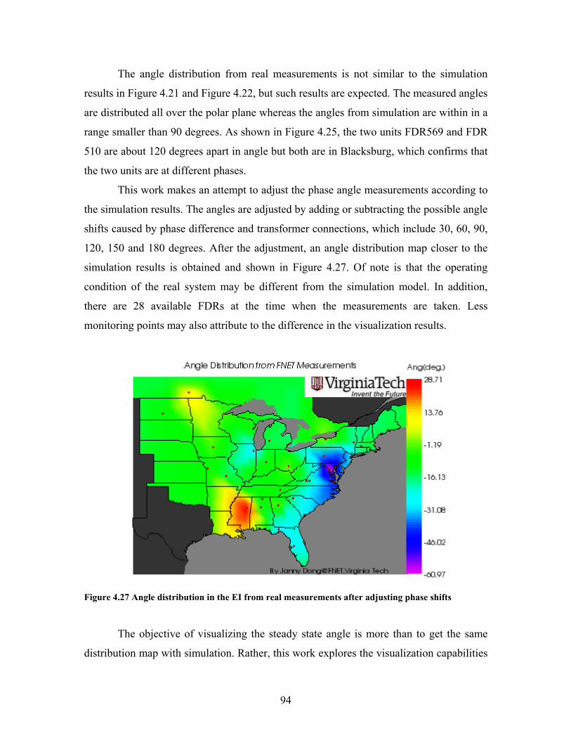
94
The angle distribution from real measurements is not similar to the simulation
results in Figure 4.21 and Figure 4.22, but such results are expected. The measured angles
are distributed all over the polar plane whereas the angles from simulation are within in a
range smaller than 90 degrees. As shown in Figure 4.25, the two units FDR569 and FDR
510 are about 120 degrees apart in angle but both are in Blacksburg, which confirms that
the two units are at different phases.
This work makes an attempt to adjust the phase angle measurements according to
the simulation results. The angles are adjusted by adding or subtracting the possible angle
shifts caused by phase difference and transformer connections, which include 30, 60, 90,
120, 150 and 180 degrees. After the adjustment, an angle distribution map closer to the
simulation results is obtained and shown in Figure 4.27. Of note is that the operating
condition of the real system may be different from the simulation model. In addition,
there are 28 available FDRs at the time when the measurements are taken. Less
monitoring points may also attribute to the difference in the visualization results.
Figure 4.27 Angle distribution in the EI from real measurements after adjusting phase shifts
The objective of visualizing the steady state angle is more than to get the same
distribution map with simulation. Rather, this work explores the visualization capabilities

95
with wide-area measurements to improve situation awareness. By monitoring the angle
distribution change over a day and during different seasons, more meaningful information
about the system operating conditions and performances can be obtained.
4.4.4 Visualization with Google Earth
Google Earth is a popular free virtual globe program developed originally by
Keyhole, Inc, a company acquired by Google in 2004. It maps the earth by superposition
of satellite images and aerial photography [56] and has the capability to show a variety of
objects such as 3D buildings by using SketchUp, a 3D modeling program; pin objects to
indicate points of interest; and line objects to display a track. Google Earth provides a
good platform to display user-defined data through Keyhole Markup Language (KML),
an Extensible Markup Language (XML)-based language for expressing geographic
annotation and visualization on Google Earth browser [57]. Although a relatively new
tool, some applications have been developed based on Google Earth to visualize energy
sources dynamically on earth [58] and wind farm [59]; to model 3D city [60]; and to
track and manage objects [61].
In light of the visualization capability of Google Earth, it is feasible to integrate
the visualization tool with the Google Earth platform to display power system
measurements. The images generated by the visualization tool can be overlaid on Google
Earth thus the animation can be displayed in Google Earth. One example is shown in
Figure 4.28, in which a snapshot of the frequency replay of the Florida outage is overlaid
on the surface of the earth by using KML. The overlaid image fits the Google map well
and can be zoomed together with the map, which automatically utilizes the geographic
information provided by Google Earth. Furthermore, Google Earth enables more
possibilities to enrich the visualization such as displaying power grid information as
different layers. The KML code for overlaying an image on Google Earth can be found in
Appendix III.
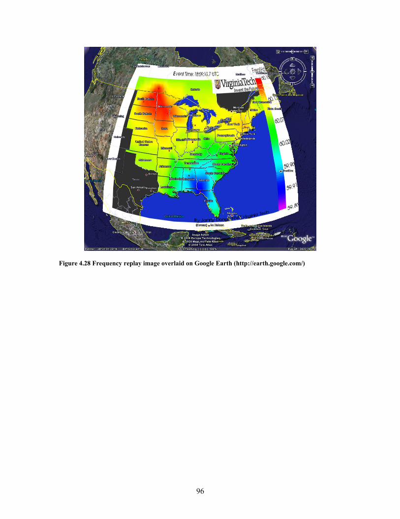
96
Figure 4.28 Frequency replay image overlaid on Google Earth (http://earth.google.com/)
97
Chapter 5 Line Trip Detection With the increase of loading of power grids and massive inter-area power
transfers enabled by the deregulation, it is very important to improve operators’ situation
awareness, which includes the knowledge of system topology. A collaborative project
between FNET and TVA is to increase the FDR density in the area, which will enable
closely monitoring of bulk transmission systems with more widely available
measurements. This chapter discusses line outage detection using measurements provided
by FNET. The line trip sensitivity and the FDR placement strategy are studied to answer
such questions as how far a line trip can be observed by the sensors and where to place
the FDRs to better observe the line trips. The characteristics of line trip disturbances are
investigated and detection algorithms based on frequency and voltage angle are
developed.
5.1 Line Trip Sensitivity Study
An ongoing project of FNET group is to deploy more sensors in the TVA system
for line trip detection study. Therefore, it is significant to know how far away a line trip
event can be observed by the sensors. It should be noted that the simulation work for the
line trip detection and identification study in Chapter 5 and 6 all focuses on the scenario
of single line trip without any fault involved since such disturbances are generally less
severe than those with faults thus less visible in measurements. Further discussion on line
trip signatures is described in detail in Chapter 6. In this chapter, the line trip sensitivity
study based on PSS/E (Power System Simulator for Engineering), a software package for
power system simulation, is carried out as follows:
(1) Select several transmission lines at different voltage levels in the TVA system.
The selected lines are listed in Table 5.1 and their locations are depicted in Figure 5.1.
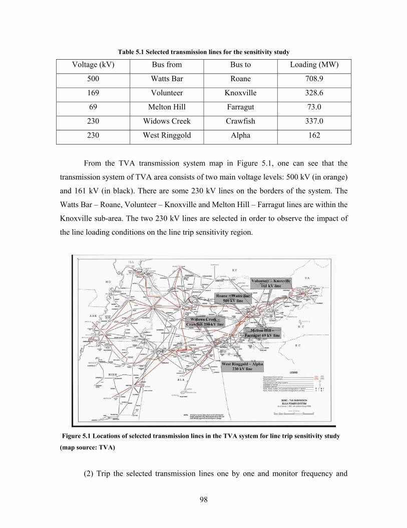
98
Table 5.1 Selected transmission lines for the sensitivity study
Voltage (kV) Bus from Bus to Loading (MW)
500 Watts Bar Roane 708.9
169 Volunteer Knoxville 328.6
69 Melton Hill Farragut 73.0
230 Widows Creek Crawfish 337.0
230 West Ringgold Alpha 162
From the TVA transmission system map in Figure 5.1, one can see that the
transmission system of TVA area consists of two main voltage levels: 500 kV (in orange)
and 161 kV (in black). There are some 230 kV lines on the borders of the system. The
Watts Bar – Roane, Volunteer – Knoxville and Melton Hill – Farragut lines are within the
Knoxville sub-area. The two 230 kV lines are selected in order to observe the impact of
the line loading conditions on the line trip sensitivity region.
Figure 5.1 Locations of selected transmission lines in the TVA system for line trip sensitivity study
(map source: TVA)
(2) Trip the selected transmission lines one by one and monitor frequency and
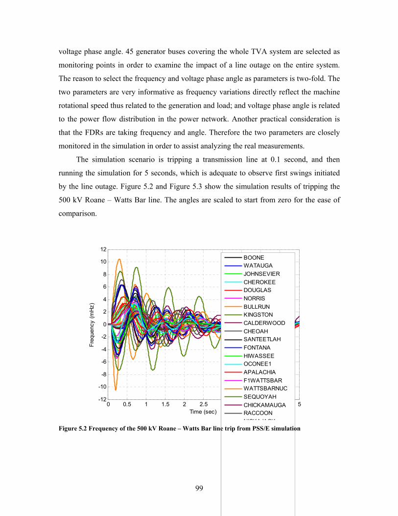
99
voltage phase angle. 45 generator buses covering the whole TVA system are selected as
monitoring points in order to examine the impact of a line outage on the entire system.
The reason to select the frequency and voltage phase angle as parameters is two-fold. The
two parameters are very informative as frequency variations directly reflect the machine
rotational speed thus related to the generation and load; and voltage phase angle is related
to the power flow distribution in the power network. Another practical consideration is
that the FDRs are taking frequency and angle. Therefore the two parameters are closely
monitored in the simulation in order to assist analyzing the real measurements.
The simulation scenario is tripping a transmission line at 0.1 second, and then
running the simulation for 5 seconds, which is adequate to observe first swings initiated
by the line outage. Figure 5.2 and Figure 5.3 show the simulation results of tripping the
500 kV Roane – Watts Bar line. The angles are scaled to start from zero for the ease of
comparison.
0 0.5 1 1.5 2 2.5 3 3.5 4 4.5 5-12
-10
-8
-6
-4
-2
0
2
4
6
8
10
12
Time (sec)
Freq
uenc
y (m
Hz)
BOONEWATAUGAJOHNSEVIERCHEROKEEDOUGLASNORRISBULLRUNKINGSTONCALDERWOODCHEOAHSANTEETLAHFONTANAHIWASSEEOCONEE1APALACHIAF1WATTSBARWATTSBARNUCSEQUOYAHCHICKAMAUGARACCOONNICKAJACK
Figure 5.2 Frequency of the 500 kV Roane – Watts Bar line trip from PSS/E simulation
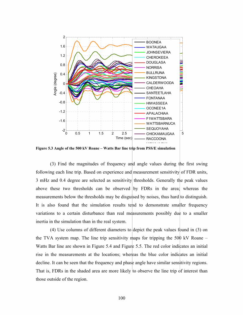
100
0 0.5 1 1.5 2 2.5 3 3.5 4 4.5 5-2
-1.6
-1.2
-0.8
-0.4
0
0.4
0.8
1.2
1.6
2
Time (sec)
Ang
le (d
egre
e)
BOONEAWATAUGAAJOHNSEVIERACHEROKEEADOUGLASANORRISABULLRUNAKINGSTONACALDERWOODACHEOAHASANTEETLAHAFONTANAAHIWASSEEAOCONEE1AAPALACHIAAF1WATTSBARAWATTSBARNUCASEQUOYAHACHICKAMAUGAARACCOONANICKAJACKA
Figure 5.3 Angle of the 500 kV Roane – Watts Bar line trip from PSS/E simulation
(3) Find the magnitudes of frequency and angle values during the first swing
following each line trip. Based on experience and measurement sensitivity of FDR units,
3 mHz and 0.4 degree are selected as sensitivity thresholds. Generally the peak values
above these two thresholds can be observed by FDRs in the area; whereas the
measurements below the thresholds may be disguised by noises, thus hard to distinguish.
It is also found that the simulation results tend to demonstrate smaller frequency
variations to a certain disturbance than real measurements possibly due to a smaller
inertia in the simulation than in the real system.
(4) Use columns of different diameters to depict the peak values found in (3) on
the TVA system map. The line trip sensitivity maps for tripping the 500 kV Roane –
Watts Bar line are shown in Figure 5.4 and Figure 5.5. The red color indicates an initial
rise in the measurements at the locations; whereas the blue color indicates an initial
decline. It can be seen that the frequency and phase angle have similar sensitivity regions.
That is, FDRs in the shaded area are more likely to observe the line trip of interest than
those outside of the region.
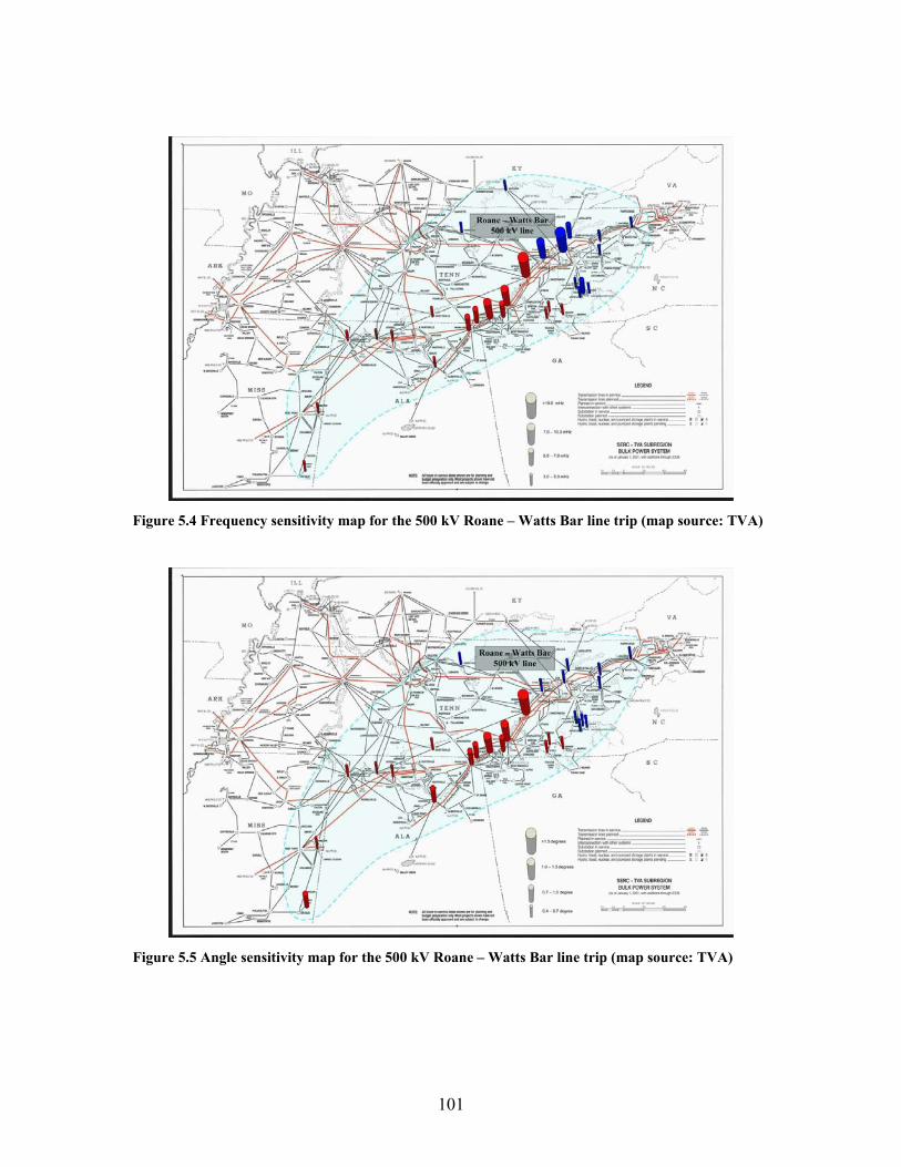
101
Figure 5.4 Frequency sensitivity map for the 500 kV Roane – Watts Bar line trip (map source: TVA)
Figure 5.5 Angle sensitivity map for the 500 kV Roane – Watts Bar line trip (map source: TVA)
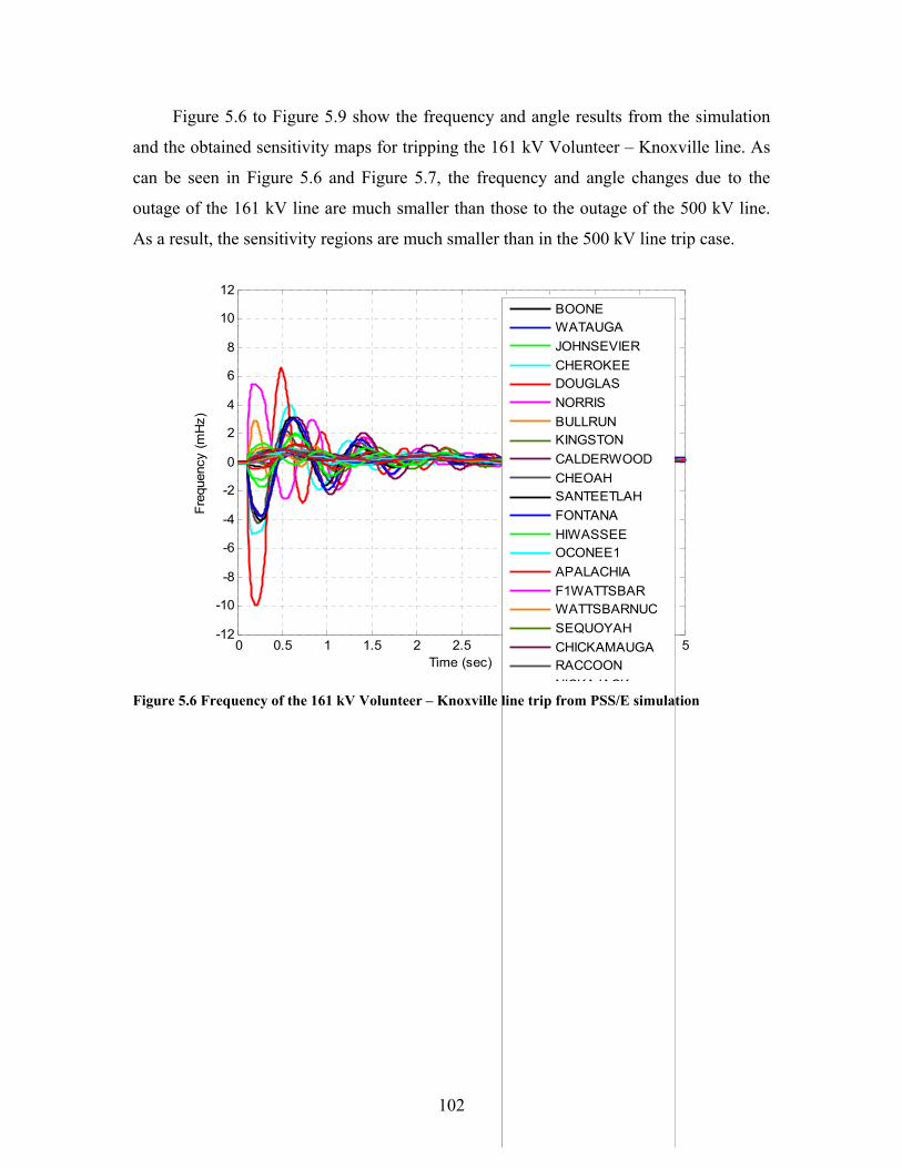
102
Figure 5.6 to Figure 5.9 show the frequency and angle results from the simulation
and the obtained sensitivity maps for tripping the 161 kV Volunteer – Knoxville line. As
can be seen in Figure 5.6 and Figure 5.7, the frequency and angle changes due to the
outage of the 161 kV line are much smaller than those to the outage of the 500 kV line.
As a result, the sensitivity regions are much smaller than in the 500 kV line trip case.
0 0.5 1 1.5 2 2.5 3 3.5 4 4.5 5-12
-10
-8
-6
-4
-2
0
2
4
6
8
10
12
Time (sec)
Freq
uenc
y (m
Hz)
BOONEWATAUGAJOHNSEVIERCHEROKEEDOUGLASNORRISBULLRUNKINGSTONCALDERWOODCHEOAHSANTEETLAHFONTANAHIWASSEEOCONEE1APALACHIAF1WATTSBARWATTSBARNUCSEQUOYAHCHICKAMAUGARACCOONNICKAJACK
Figure 5.6 Frequency of the 161 kV Volunteer – Knoxville line trip from PSS/E simulation
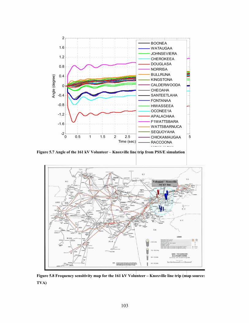
103
0 0.5 1 1.5 2 2.5 3 3.5 4 4.5 5-2
-1.6
-1.2
-0.8
-0.4
0
0.4
0.8
1.2
1.6
2
Time (sec)
Ang
le (d
egre
e)
BOONEAWATAUGAAJOHNSEVIERACHEROKEEADOUGLASANORRISABULLRUNAKINGSTONACALDERWOODACHEOAHASANTEETLAHAFONTANAAHIWASSEEAOCONEE1AAPALACHIAAF1WATTSBARAWATTSBARNUCASEQUOYAHACHICKAMAUGAARACCOONANICKAJACKA
Figure 5.7 Angle of the 161 kV Volunteer – Knoxville line trip from PSS/E simulation
Figure 5.8 Frequency sensitivity map for the 161 kV Volunteer – Knoxville line trip (map source:
TVA)
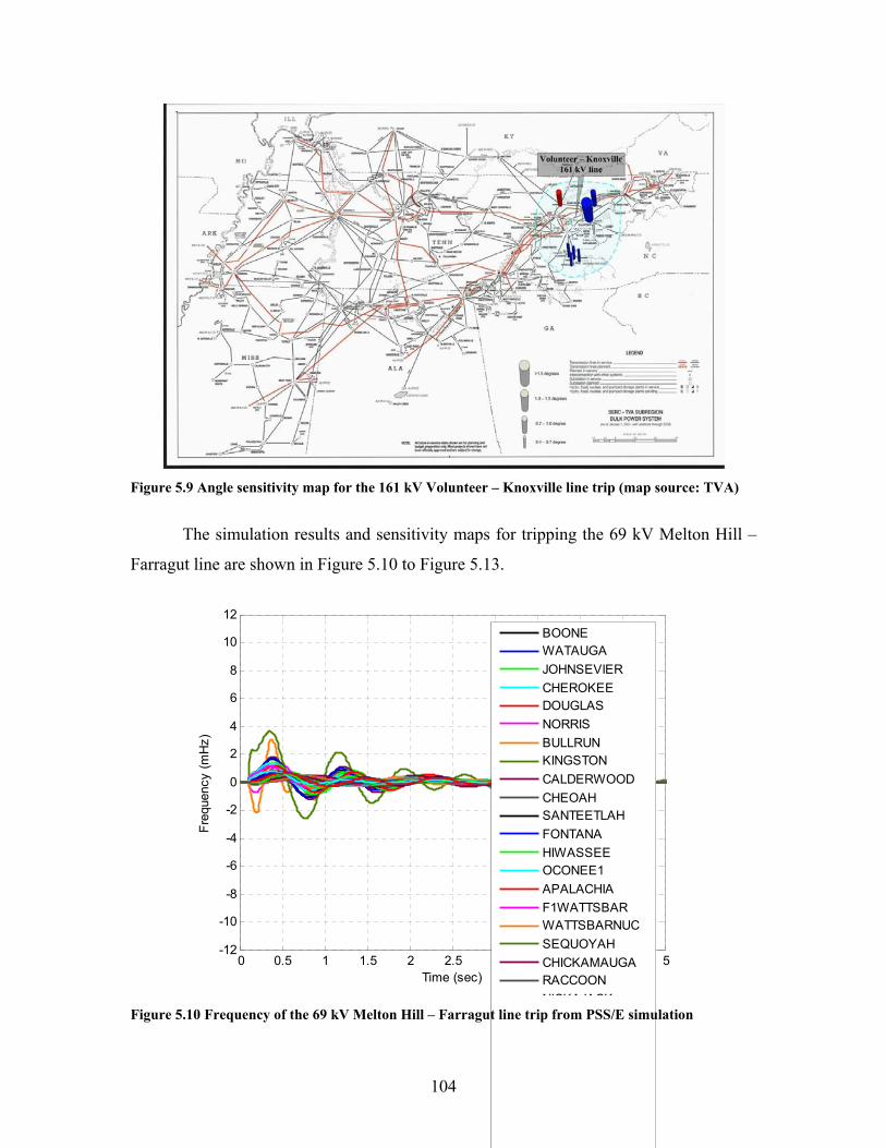
104
Figure 5.9 Angle sensitivity map for the 161 kV Volunteer – Knoxville line trip (map source: TVA)
The simulation results and sensitivity maps for tripping the 69 kV Melton Hill –
Farragut line are shown in Figure 5.10 to Figure 5.13.
0 0.5 1 1.5 2 2.5 3 3.5 4 4.5 5-12
-10
-8
-6
-4
-2
0
2
4
6
8
10
12
Time (sec)
Freq
uenc
y (m
Hz)
BOONEWATAUGAJOHNSEVIERCHEROKEEDOUGLASNORRISBULLRUNKINGSTONCALDERWOODCHEOAHSANTEETLAHFONTANAHIWASSEEOCONEE1APALACHIAF1WATTSBARWATTSBARNUCSEQUOYAHCHICKAMAUGARACCOONNICKAJACK
Figure 5.10 Frequency of the 69 kV Melton Hill – Farragut line trip from PSS/E simulation
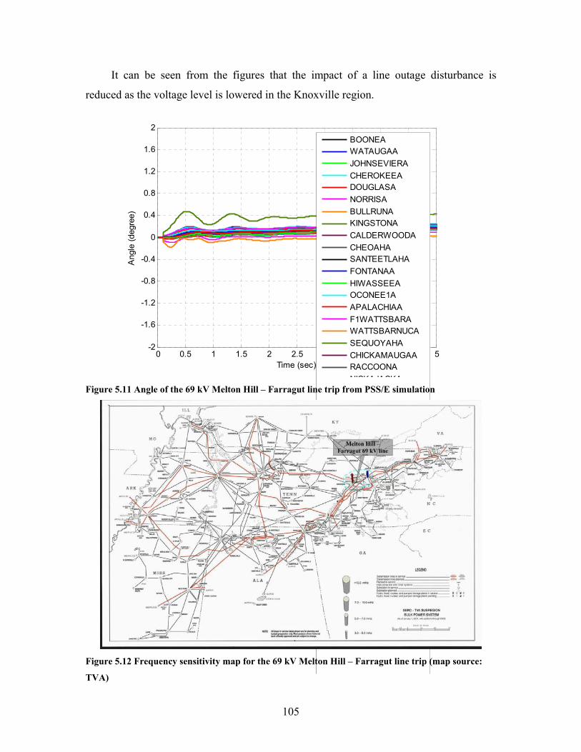
105
It can be seen from the figures that the impact of a line outage disturbance is
reduced as the voltage level is lowered in the Knoxville region.
0 0.5 1 1.5 2 2.5 3 3.5 4 4.5 5-2
-1.6
-1.2
-0.8
-0.4
0
0.4
0.8
1.2
1.6
2
Time (sec)
Ang
le (d
egre
e)BOONEAWATAUGAAJOHNSEVIERACHEROKEEADOUGLASANORRISABULLRUNAKINGSTONACALDERWOODACHEOAHASANTEETLAHAFONTANAAHIWASSEEAOCONEE1AAPALACHIAAF1WATTSBARAWATTSBARNUCASEQUOYAHACHICKAMAUGAARACCOONANICKAJACKA
Figure 5.11 Angle of the 69 kV Melton Hill – Farragut line trip from PSS/E simulation
Figure 5.12 Frequency sensitivity map for the 69 kV Melton Hill – Farragut line trip (map source:
TVA)
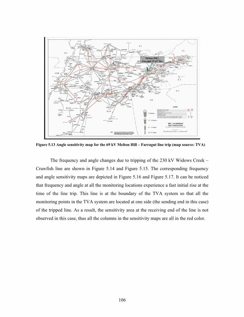
106
Figure 5.13 Angle sensitivity map for the 69 kV Melton Hill – Farragut line trip (map source: TVA)
The frequency and angle changes due to tripping of the 230 kV Widows Creek –
Crawfish line are shown in Figure 5.14 and Figure 5.15. The corresponding frequency
and angle sensitivity maps are depicted in Figure 5.16 and Figure 5.17. It can be noticed
that frequency and angle at all the monitoring locations experience a fast initial rise at the
time of the line trip. This line is at the boundary of the TVA system so that all the
monitoring points in the TVA system are located at one side (the sending end in this case)
of the tripped line. As a result, the sensitivity area at the receiving end of the line is not
observed in this case, thus all the columns in the sensitivity maps are all in the red color.
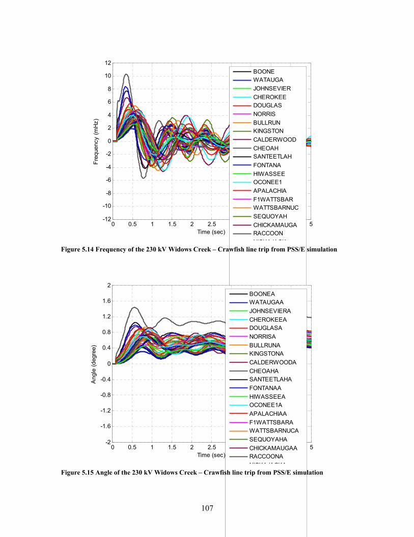
107
0 0.5 1 1.5 2 2.5 3 3.5 4 4.5 5-12
-10
-8
-6
-4
-2
0
2
4
6
8
10
12
Time (sec)
Freq
uenc
y (m
Hz)
BOONEWATAUGAJOHNSEVIERCHEROKEEDOUGLASNORRISBULLRUNKINGSTONCALDERWOODCHEOAHSANTEETLAHFONTANAHIWASSEEOCONEE1APALACHIAF1WATTSBARWATTSBARNUCSEQUOYAHCHICKAMAUGARACCOONNICKAJACK
Figure 5.14 Frequency of the 230 kV Widows Creek – Crawfish line trip from PSS/E simulation
0 0.5 1 1.5 2 2.5 3 3.5 4 4.5 5-2
-1.6
-1.2
-0.8
-0.4
0
0.4
0.8
1.2
1.6
2
Time (sec)
Ang
le (d
egre
e)
BOONEAWATAUGAAJOHNSEVIERACHEROKEEADOUGLASANORRISABULLRUNAKINGSTONACALDERWOODACHEOAHASANTEETLAHAFONTANAAHIWASSEEAOCONEE1AAPALACHIAAF1WATTSBARAWATTSBARNUCASEQUOYAHACHICKAMAUGAARACCOONANICKAJACKA
Figure 5.15 Angle of the 230 kV Widows Creek – Crawfish line trip from PSS/E simulation
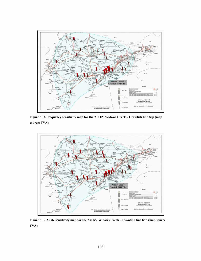
108
Figure 5.16 Frequency sensitivity map for the 230 kV Widows Creek – Crawfish line trip (map
source: TVA)
Figure 5.17 Angle sensitivity map for the 230 kV Widows Creek – Crawfish line trip (map source:
TVA)
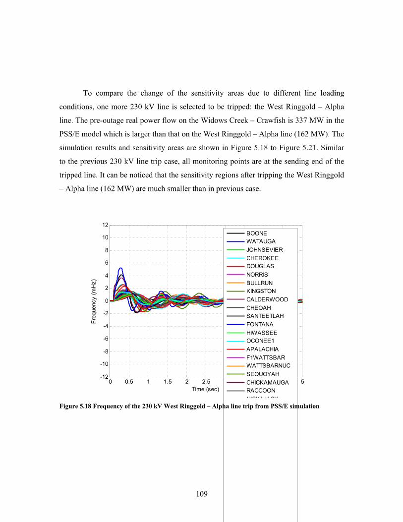
109
To compare the change of the sensitivity areas due to different line loading
conditions, one more 230 kV line is selected to be tripped: the West Ringgold – Alpha
line. The pre-outage real power flow on the Widows Creek – Crawfish is 337 MW in the
PSS/E model which is larger than that on the West Ringgold – Alpha line (162 MW). The
simulation results and sensitivity areas are shown in Figure 5.18 to Figure 5.21. Similar
to the previous 230 kV line trip case, all monitoring points are at the sending end of the
tripped line. It can be noticed that the sensitivity regions after tripping the West Ringgold
– Alpha line (162 MW) are much smaller than in previous case.
0 0.5 1 1.5 2 2.5 3 3.5 4 4.5 5-12
-10
-8
-6
-4
-2
0
2
4
6
8
10
12
Time (sec)
Freq
uenc
y (m
Hz)
BOONEWATAUGAJOHNSEVIERCHEROKEEDOUGLASNORRISBULLRUNKINGSTONCALDERWOODCHEOAHSANTEETLAHFONTANAHIWASSEEOCONEE1APALACHIAF1WATTSBARWATTSBARNUCSEQUOYAHCHICKAMAUGARACCOONNICKAJACK
Figure 5.18 Frequency of the 230 kV West Ringgold – Alpha line trip from PSS/E simulation
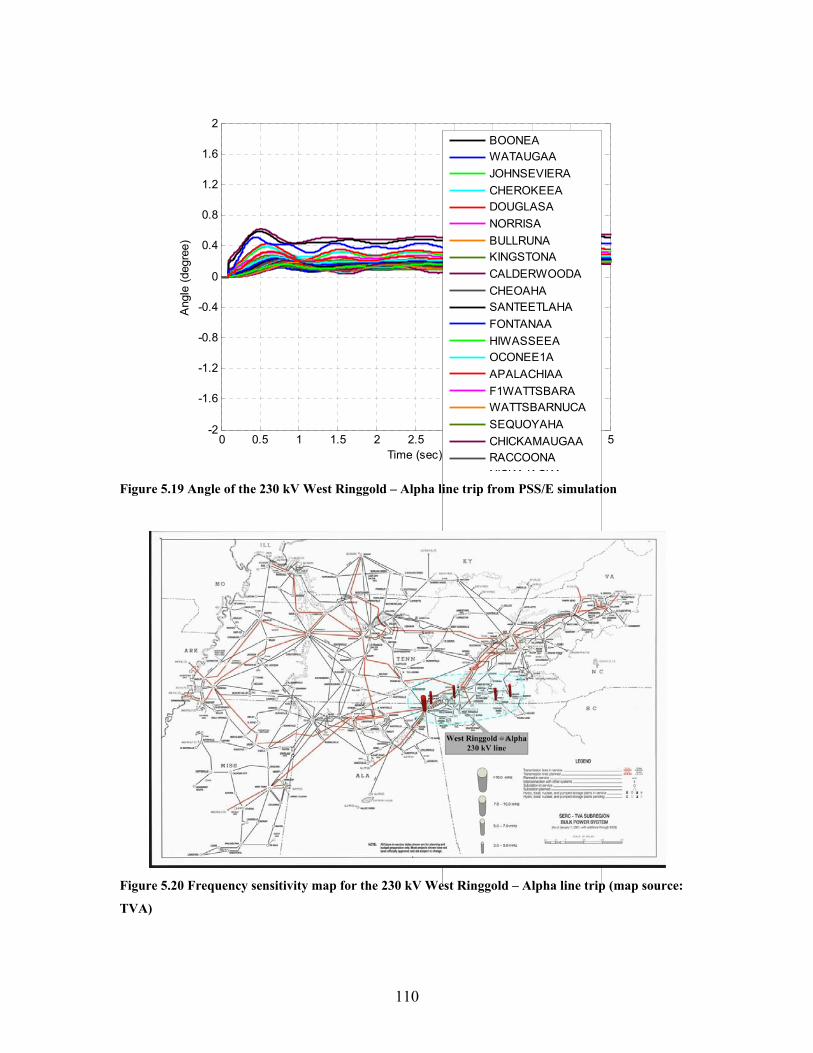
110
0 0.5 1 1.5 2 2.5 3 3.5 4 4.5 5-2
-1.6
-1.2
-0.8
-0.4
0
0.4
0.8
1.2
1.6
2
Time (sec)
Ang
le (d
egre
e)
BOONEAWATAUGAAJOHNSEVIERACHEROKEEADOUGLASANORRISABULLRUNAKINGSTONACALDERWOODACHEOAHASANTEETLAHAFONTANAAHIWASSEEAOCONEE1AAPALACHIAAF1WATTSBARAWATTSBARNUCASEQUOYAHACHICKAMAUGAARACCOONANICKAJACKA
Figure 5.19 Angle of the 230 kV West Ringgold – Alpha line trip from PSS/E simulation
Figure 5.20 Frequency sensitivity map for the 230 kV West Ringgold – Alpha line trip (map source:
TVA)
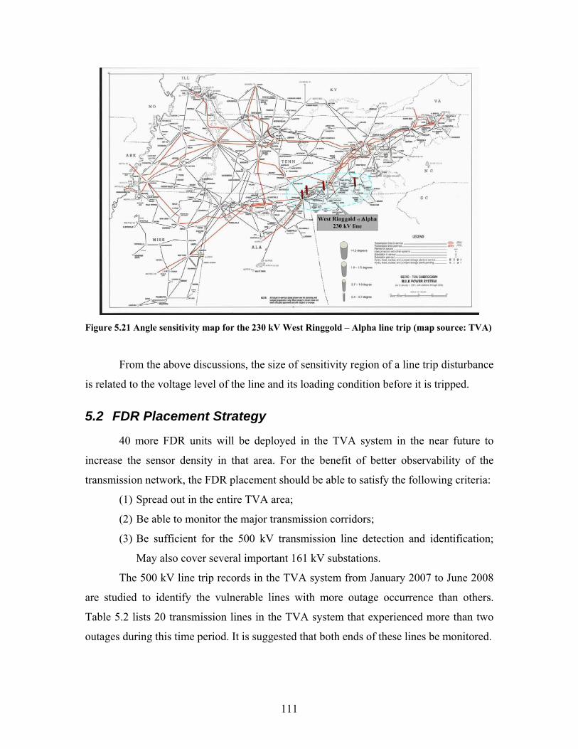
111
Figure 5.21 Angle sensitivity map for the 230 kV West Ringgold – Alpha line trip (map source: TVA)
From the above discussions, the size of sensitivity region of a line trip disturbance
is related to the voltage level of the line and its loading condition before it is tripped.
5.2 FDR Placement Strategy
40 more FDR units will be deployed in the TVA system in the near future to
increase the sensor density in that area. For the benefit of better observability of the
transmission network, the FDR placement should be able to satisfy the following criteria:
(1) Spread out in the entire TVA area;
(2) Be able to monitor the major transmission corridors;
(3) Be sufficient for the 500 kV transmission line detection and identification;
May also cover several important 161 kV substations.
The 500 kV line trip records in the TVA system from January 2007 to June 2008
are studied to identify the vulnerable lines with more outage occurrence than others.
Table 5.2 lists 20 transmission lines in the TVA system that experienced more than two
outages during this time period. It is suggested that both ends of these lines be monitored.
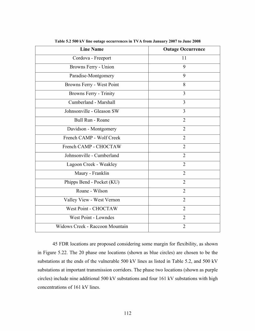
112
Table 5.2 500 kV line outage occurrences in TVA from January 2007 to June 2008
Line Name Outage Occurrence
Cordova - Freeport 11
Browns Ferry - Union 9
Paradise-Montgomery 9
Browns Ferry - West Point 8
Browns Ferry - Trinity 3
Cumberland - Marshall 3
Johnsonville - Gleason SW 3
Bull Run - Roane 2
Davidson - Montgomery 2
French CAMP - Wolf Creek 2
French CAMP - CHOCTAW 2
Johnsonville - Cumberland 2
Lagoon Creek - Weakley 2
Maury - Franklin 2
Phipps Bend - Pocket (KU) 2
Roane - Wilson 2
Valley View - West Vernon 2
West Point - CHOCTAW 2
West Point - Lowndes 2
Widows Creek - Raccoon Mountain 2
45 FDR locations are proposed considering some margin for flexibility, as shown
in Figure 5.22. The 20 phase one locations (shown as blue circles) are chosen to be the
substations at the ends of the vulnerable 500 kV lines as listed in Table 5.2, and 500 kV
substations at important transmission corridors. The phase two locations (shown as purple
circles) include nine additional 500 kV substations and four 161 kV substations with high
concentrations of 161 kV lines.
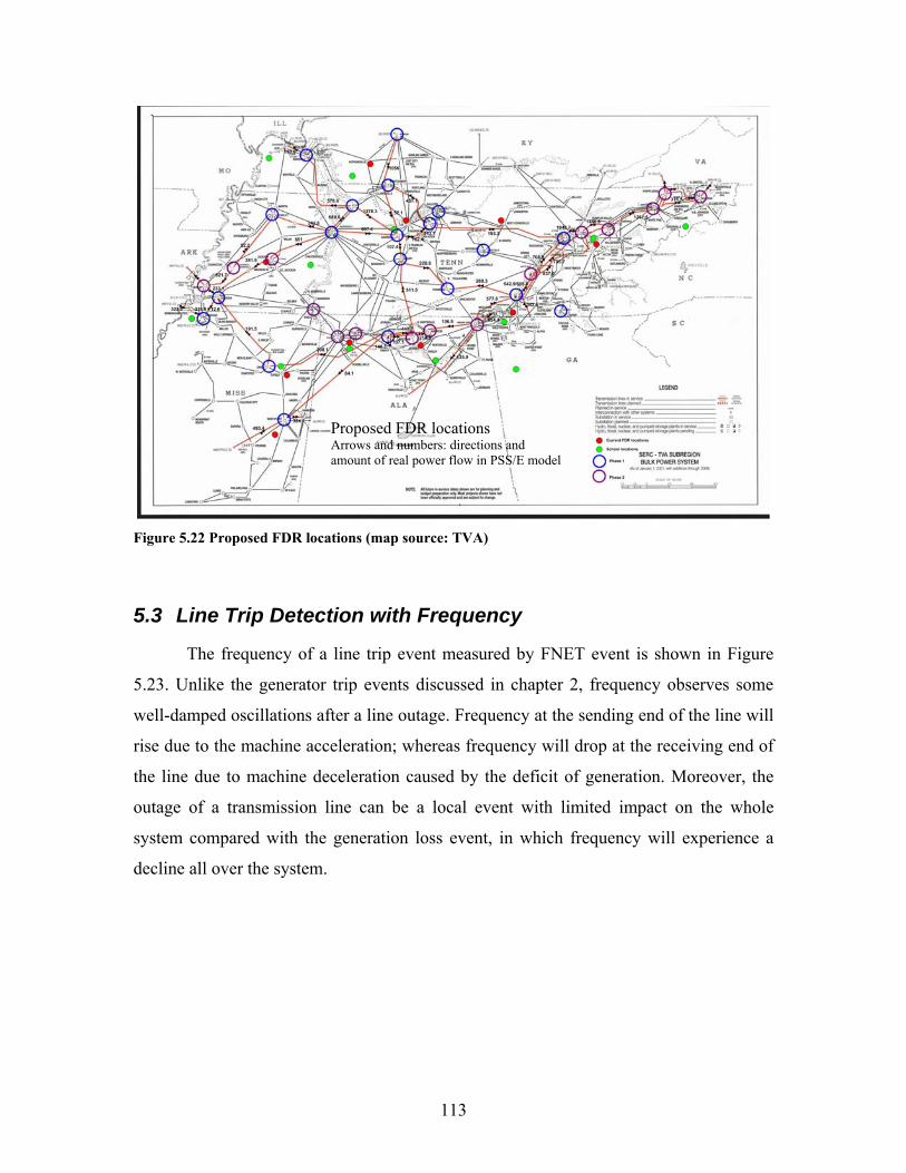
113
Figure 5.22 Proposed FDR locations (map source: TVA)
5.3 Line Trip Detection with Frequency
The frequency of a line trip event measured by FNET event is shown in Figure
5.23. Unlike the generator trip events discussed in chapter 2, frequency observes some
well-damped oscillations after a line outage. Frequency at the sending end of the line will
rise due to the machine acceleration; whereas frequency will drop at the receiving end of
the line due to machine deceleration caused by the deficit of generation. Moreover, the
outage of a transmission line can be a local event with limited impact on the whole
system compared with the generation loss event, in which frequency will experience a
decline all over the system.
Proposed FDR locations Arrows and numbers: directions and amount of real power flow in PSS/E model
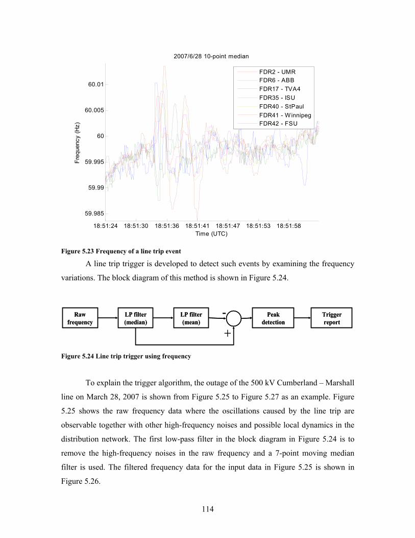
114
Figure 5.23 Frequency of a line trip event
A line trip trigger is developed to detect such events by examining the frequency
variations. The block diagram of this method is shown in Figure 5.24.
Raw frequency
LP filter (median)
LP filter (mean)
Peak detection
Trigger report
+
-Raw frequency
LP filter (median)
LP filter (mean)
Peak detection
Trigger report
+
-
Figure 5.24 Line trip trigger using frequency
To explain the trigger algorithm, the outage of the 500 kV Cumberland – Marshall
line on March 28, 2007 is shown from Figure 5.25 to Figure 5.27 as an example. Figure
5.25 shows the raw frequency data where the oscillations caused by the line trip are
observable together with other high-frequency noises and possible local dynamics in the
distribution network. The first low-pass filter in the block diagram in Figure 5.24 is to
remove the high-frequency noises in the raw frequency and a 7-point moving median
filter is used. The filtered frequency data for the input data in Figure 5.25 is shown in
Figure 5.26.
18:51:24 18:51:30 18:51:36 18:51:41 18:51:47 18:51:53 18:51:58
59.985
59.99
59.995
60
60.005
60.01
Time (UTC)
Freq
uenc
y (H
z)
2007/6/28 10-point median
FDR2 - UMRFDR6 - ABBFDR17 - TVA4FDR35 - ISUFDR40 - StPaulFDR41 - WinnipegFDR42 - FSU
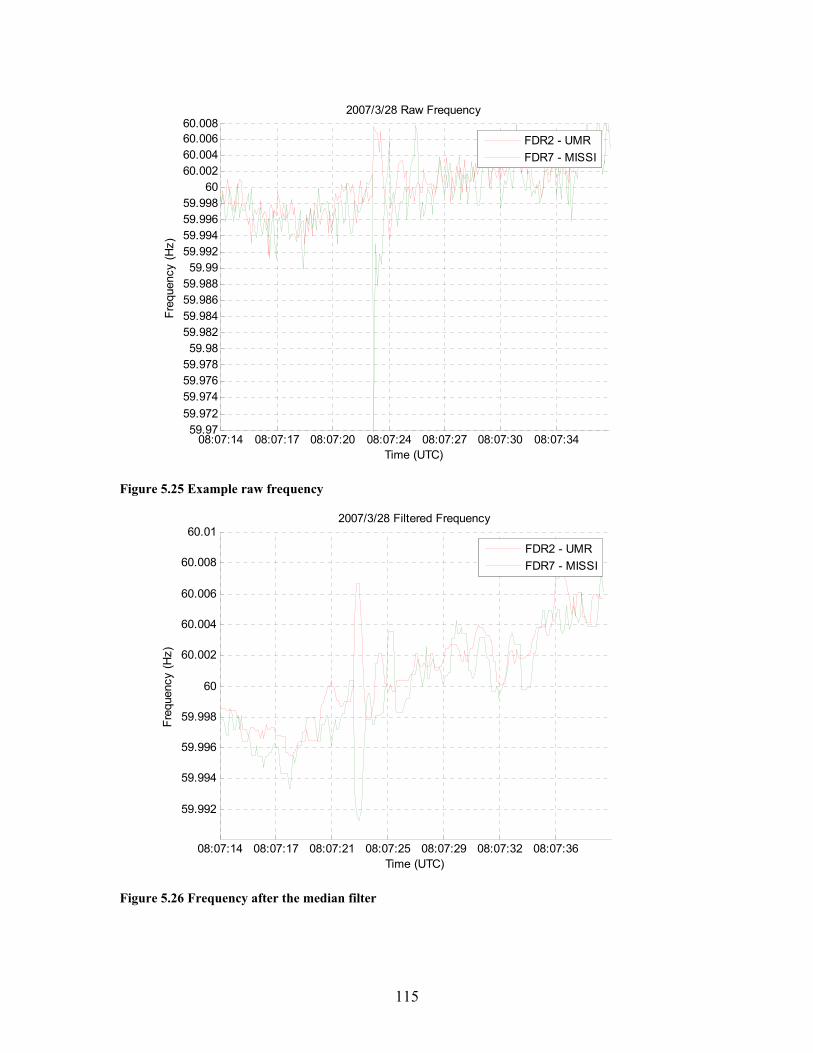
115
08:07:14 08:07:17 08:07:20 08:07:24 08:07:27 08:07:30 08:07:3459.97
59.97259.97459.97659.97859.98
59.98259.98459.98659.98859.99
59.99259.99459.99659.998
6060.00260.00460.00660.008
Time (UTC)
Freq
uenc
y (H
z)
2007/3/28 Raw Frequency
FDR2 - UMRFDR7 - MISSI
Figure 5.25 Example raw frequency
08:07:14 08:07:17 08:07:21 08:07:25 08:07:29 08:07:32 08:07:36
59.992
59.994
59.996
59.998
60
60.002
60.004
60.006
60.008
60.01
Time (UTC)
Freq
uenc
y (H
z)
2007/3/28 Filtered Frequency
FDR2 - UMRFDR7 - MISSI
Figure 5.26 Frequency after the median filter
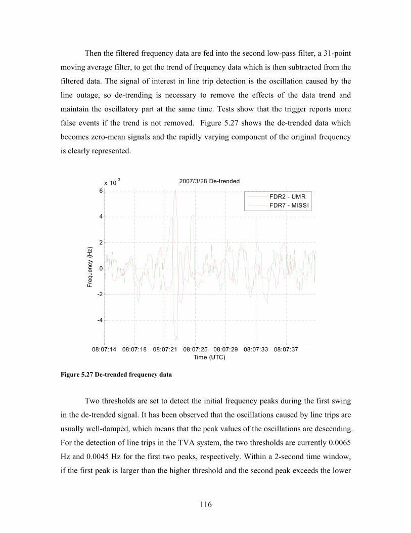
116
Then the filtered frequency data are fed into the second low-pass filter, a 31-point
moving average filter, to get the trend of frequency data which is then subtracted from the
filtered data. The signal of interest in line trip detection is the oscillation caused by the
line outage, so de-trending is necessary to remove the effects of the data trend and
maintain the oscillatory part at the same time. Tests show that the trigger reports more
false events if the trend is not removed. Figure 5.27 shows the de-trended data which
becomes zero-mean signals and the rapidly varying component of the original frequency
is clearly represented.
Figure 5.27 De-trended frequency data
Two thresholds are set to detect the initial frequency peaks during the first swing
in the de-trended signal. It has been observed that the oscillations caused by line trips are
usually well-damped, which means that the peak values of the oscillations are descending.
For the detection of line trips in the TVA system, the two thresholds are currently 0.0065
Hz and 0.0045 Hz for the first two peaks, respectively. Within a 2-second time window,
if the first peak is larger than the higher threshold and the second peak exceeds the lower
08:07:14 08:07:18 08:07:21 08:07:25 08:07:29 08:07:33 08:07:37
-4
-2
0
2
4
6x 10⁻³
Time (UTC)
Freq
uenc
y (H
z)
2007/3/28 De-trended
FDR2 - UMRFDR7 - MISSI
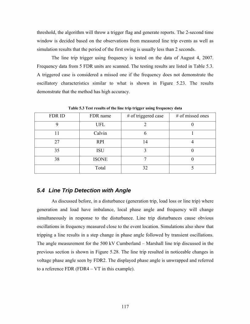
117
threshold, the algorithm will throw a trigger flag and generate reports. The 2-second time
window is decided based on the observations from measured line trip events as well as
simulation results that the period of the first swing is usually less than 2 seconds.
The line trip trigger using frequency is tested on the data of August 4, 2007.
Frequency data from 5 FDR units are scanned. The testing results are listed in Table 5.3.
A triggered case is considered a missed one if the frequency does not demonstrate the
oscillatory characteristics similar to what is shown in Figure 5.23. The results
demonstrate that the method has high accuracy.
Table 5.3 Test results of the line trip trigger using frequency data
FDR ID FDR name # of triggered case # of missed ones
9 UFL 2 0
11 Calvin 6 1
27 RPI 14 4
35 ISU 3 0
38 ISONE 7 0
Total 32 5
5.4 Line Trip Detection with Angle
As discussed before, in a disturbance (generation trip, load loss or line trip) where
generation and load have imbalance, local phase angle and frequency will change
simultaneously in response to the disturbance. Line trip disturbances cause obvious
oscillations in frequency measured close to the event location. Simulations also show that
tripping a line results in a step change in phase angle followed by transient oscillations.
The angle measurement for the 500 kV Cumberland – Marshall line trip discussed in the
previous section is shown in Figure 5.28. The line trip resulted in noticeable changes in
voltage phase angle seen by FDR2. The displayed phase angle is unwrapped and referred
to a reference FDR (FDR4 – VT in this example).
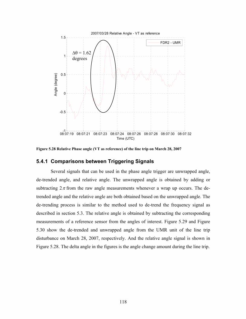
118
08:07:19 08:07:21 08:07:23 08:07:24 08:07:26 08:07:28 08:07:30 08:07:32-1
-0.5
0
0.5
1
1.5
Time (UTC)
Ang
le (d
egre
e)
2007/03/28 Relative Angle - VT as reference
FDR2 - UMR
Figure 5.28 Relative Phase angle (VT as reference) of the line trip on March 28, 2007
5.4.1 Comparisons between Triggering Signals
Several signals that can be used in the phase angle trigger are unwrapped angle,
de-trended angle, and relative angle. The unwrapped angle is obtained by adding or
subtracting 2π from the raw angle measurements whenever a wrap up occurs. The de-
trended angle and the relative angle are both obtained based on the unwrapped angle. The
de-trending process is similar to the method used to de-trend the frequency signal as
described in section 5.3. The relative angle is obtained by subtracting the corresponding
measurements of a reference sensor from the angles of interest. Figure 5.29 and Figure
5.30 show the de-trended and unwrapped angle from the UMR unit of the line trip
disturbance on March 28, 2007, respectively. And the relative angle signal is shown in
Figure 5.28. The delta angle in the figures is the angle change amount during the line trip.
∆θ = 1.62 degrees
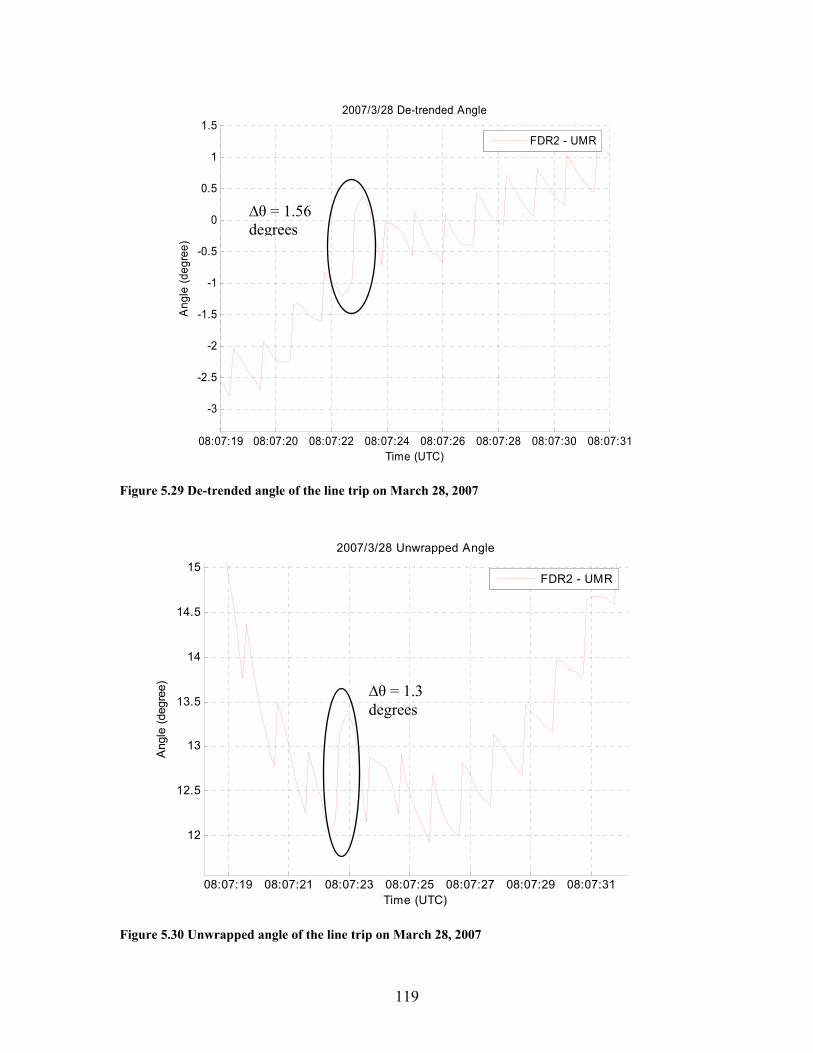
119
08:07:19 08:07:20 08:07:22 08:07:24 08:07:26 08:07:28 08:07:30 08:07:31
-3
-2.5
-2
-1.5
-1
-0.5
0
0.5
1
1.5
Time (UTC)
Ang
le (d
egre
e)
2007/3/28 De-trended Angle
FDR2 - UMR
Figure 5.29 De-trended angle of the line trip on March 28, 2007
Figure 5.30 Unwrapped angle of the line trip on March 28, 2007
08:07:19 08:07:21 08:07:23 08:07:25 08:07:27 08:07:29 08:07:31
12
12.5
13
13.5
14
14.5
15
Time (UTC)
Ang
le (d
egre
e)
2007/3/28 Unwrapped Angle
FDR2 - UMR
∆θ = 1.3 degrees
∆θ = 1.56 degrees
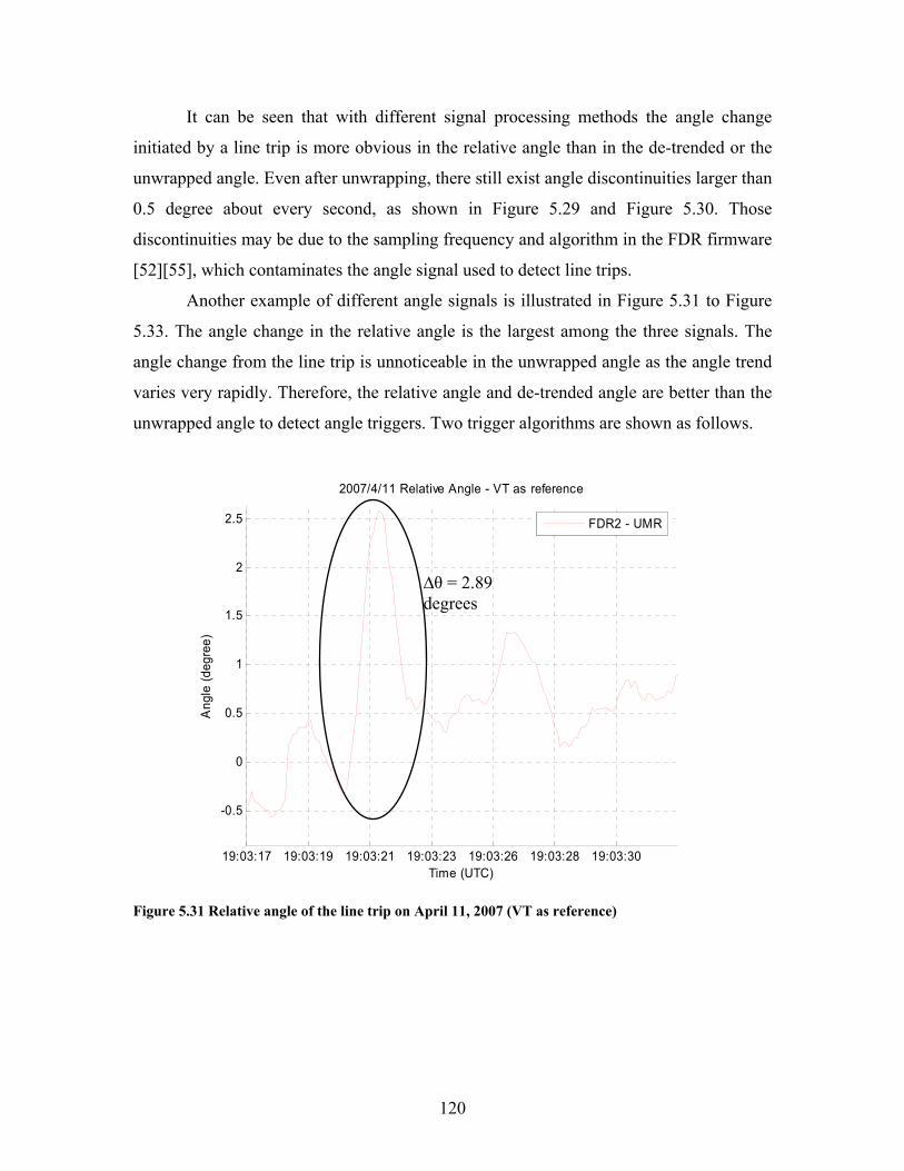
120
It can be seen that with different signal processing methods the angle change
initiated by a line trip is more obvious in the relative angle than in the de-trended or the
unwrapped angle. Even after unwrapping, there still exist angle discontinuities larger than
0.5 degree about every second, as shown in Figure 5.29 and Figure 5.30. Those
discontinuities may be due to the sampling frequency and algorithm in the FDR firmware
[52][55], which contaminates the angle signal used to detect line trips.
Another example of different angle signals is illustrated in Figure 5.31 to Figure
5.33. The angle change in the relative angle is the largest among the three signals. The
angle change from the line trip is unnoticeable in the unwrapped angle as the angle trend
varies very rapidly. Therefore, the relative angle and de-trended angle are better than the
unwrapped angle to detect angle triggers. Two trigger algorithms are shown as follows.
19:03:17 19:03:19 19:03:21 19:03:23 19:03:26 19:03:28 19:03:30
-0.5
0
0.5
1
1.5
2
2.5
Time (UTC)
Ang
le (d
egre
e)
2007/4/11 Relative Angle - VT as reference
FDR2 - UMR
Figure 5.31 Relative angle of the line trip on April 11, 2007 (VT as reference)
∆θ = 2.89 degrees
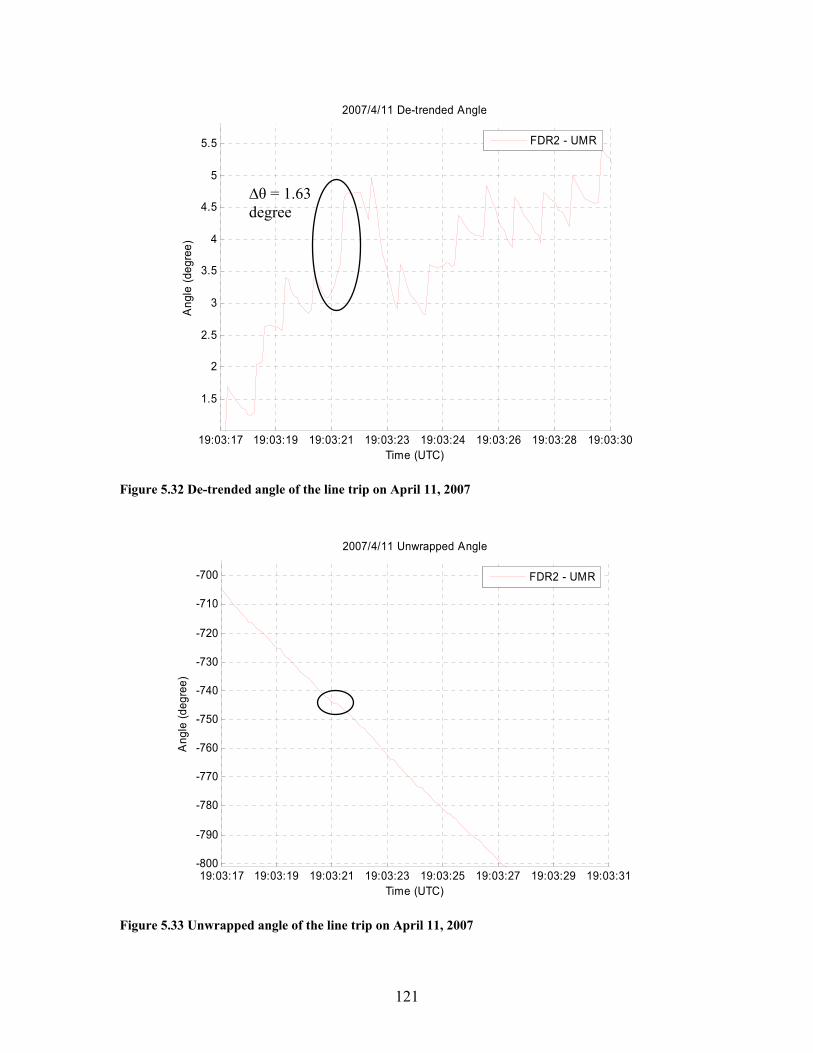
121
19:03:17 19:03:19 19:03:21 19:03:23 19:03:24 19:03:26 19:03:28 19:03:30
1.5
2
2.5
3
3.5
4
4.5
5
5.5
Time (UTC)
Ang
le (d
egre
e)
2007/4/11 De-trended Angle
FDR2 - UMR
Figure 5.32 De-trended angle of the line trip on April 11, 2007
19:03:17 19:03:19 19:03:21 19:03:23 19:03:25 19:03:27 19:03:29 19:03:31-800
-790
-780
-770
-760
-750
-740
-730
-720
-710
-700
Time (UTC)
Ang
le (d
egre
e)
2007/4/11 Unwrapped Angle
FDR2 - UMR
Figure 5.33 Unwrapped angle of the line trip on April 11, 2007
∆θ = 1.63 degree
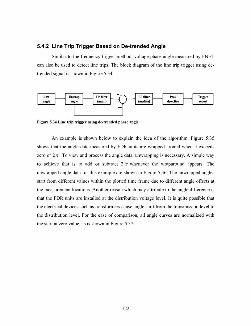
122
5.4.2 Line Trip Trigger Based on De-trended Angle
Similar to the frequency trigger method, voltage phase angle measured by FNET
can also be used to detect line trips. The block diagram of the line trip trigger using de-
trended signal is shown in Figure 5.34.
Raw angle
Unwrap angle
LP filter (mean)
Peak detection
Trigger report
+
- LP filter (median)
Raw angle
Unwrap angle
LP filter (mean)
Peak detection
Trigger report
+
- LP filter (median)
Figure 5.34 Line trip trigger using de-trended phase angle
An example is shown below to explain the idea of the algorithm. Figure 5.35
shows that the angle data measured by FDR units are wrapped around when it exceeds
zero or 2π . To view and process the angle data, unwrapping is necessary. A simple way
to achieve that is to add or subtract 2 π whenever the wraparound appears. The
unwrapped angle data for this example are shown in Figure 5.36. The unwrapped angles
start from different values within the plotted time frame due to different angle offsets at
the measurement locations. Another reason which may attribute to the angle difference is
that the FDR units are installed at the distribution voltage level. It is quite possible that
the electrical devices such as transformers cause angle shift from the transmission level to
the distribution level. For the ease of comparison, all angle curves are normalized with
the start at zero value, as is shown in Figure 5.37.
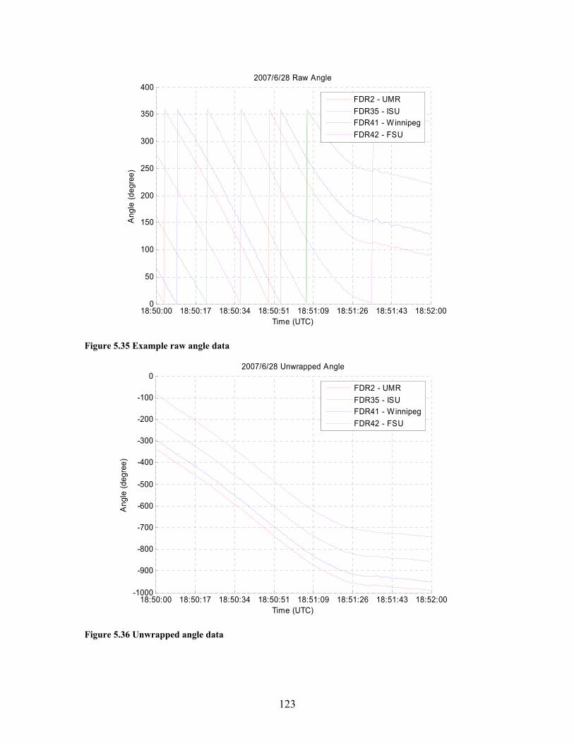
123
18:50:00 18:50:17 18:50:34 18:50:51 18:51:09 18:51:26 18:51:43 18:52:000
50
100
150
200
250
300
350
400
Time (UTC)
Ang
le (d
egre
e)
2007/6/28 Raw Angle
FDR2 - UMRFDR35 - ISUFDR41 - WinnipegFDR42 - FSU
Figure 5.35 Example raw angle data
18:50:00 18:50:17 18:50:34 18:50:51 18:51:09 18:51:26 18:51:43 18:52:00-1000
-900
-800
-700
-600
-500
-400
-300
-200
-100
0
Time (UTC)
Ang
le (d
egre
e)
2007/6/28 Unwrapped Angle
FDR2 - UMRFDR35 - ISUFDR41 - WinnipegFDR42 - FSU
Figure 5.36 Unwrapped angle data
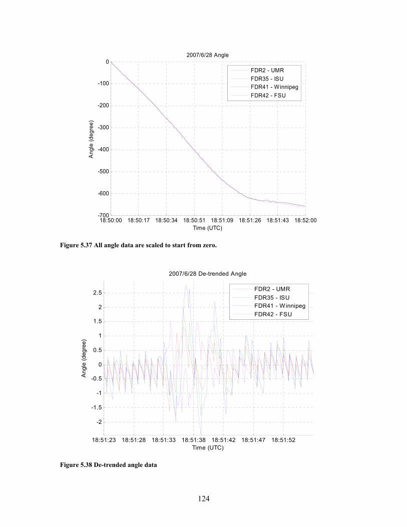
124
18:50:00 18:50:17 18:50:34 18:50:51 18:51:09 18:51:26 18:51:43 18:52:00-700
-600
-500
-400
-300
-200
-100
0
Time (UTC)
Ang
le (d
egre
e)
2007/6/28 Angle
FDR2 - UMRFDR35 - ISUFDR41 - WinnipegFDR42 - FSU
Figure 5.37 All angle data are scaled to start from zero.
Figure 5.38 De-trended angle data
18:51:23 18:51:28 18:51:33 18:51:38 18:51:42 18:51:47 18:51:52
-2
-1.5
-1
-0.5
0
0.5
1
1.5
2
2.5
Time (UTC)
Ang
le (d
egre
e)
2007/6/28 De-trended Angle
FDR2 - UMRFDR35 - ISUFDR41 - WinnipegFDR42 - FSU
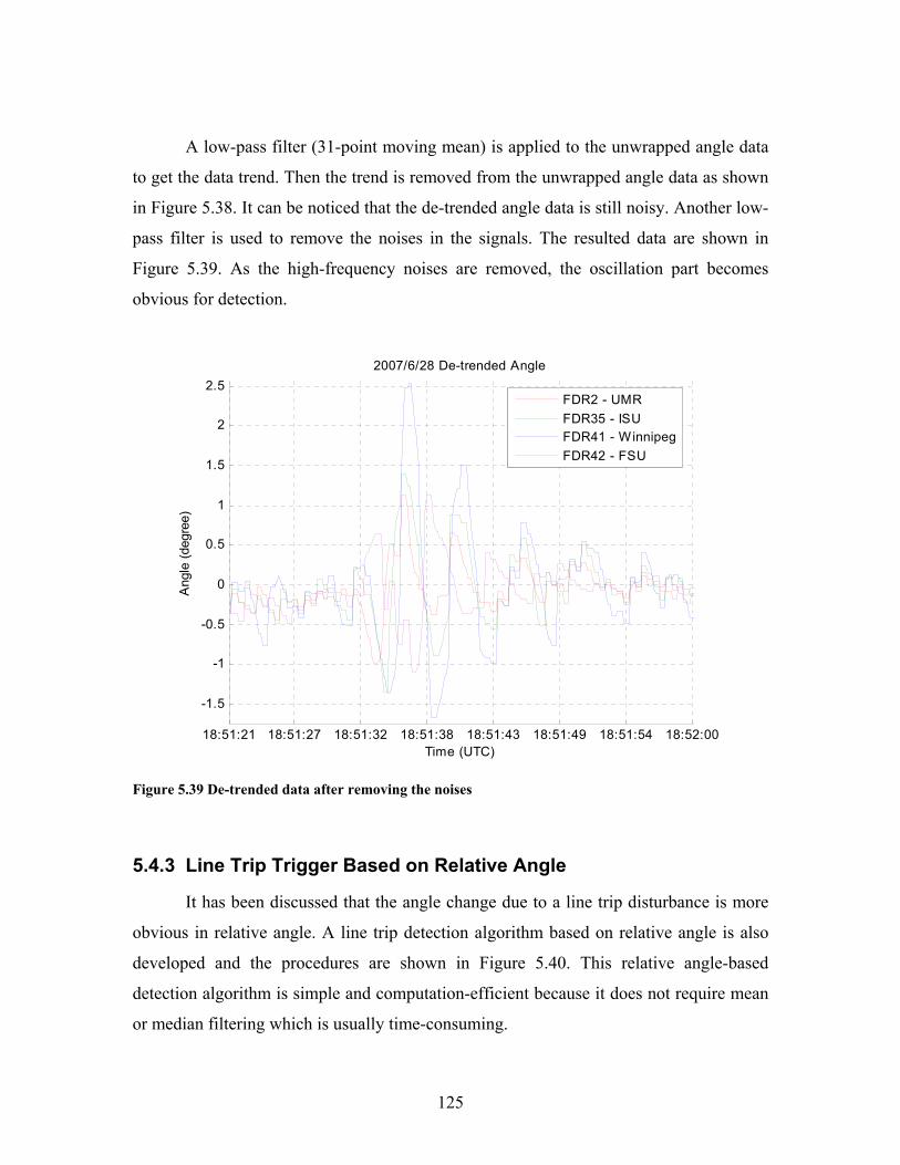
125
A low-pass filter (31-point moving mean) is applied to the unwrapped angle data
to get the data trend. Then the trend is removed from the unwrapped angle data as shown
in Figure 5.38. It can be noticed that the de-trended angle data is still noisy. Another low-
pass filter is used to remove the noises in the signals. The resulted data are shown in
Figure 5.39. As the high-frequency noises are removed, the oscillation part becomes
obvious for detection.
Figure 5.39 De-trended data after removing the noises
5.4.3 Line Trip Trigger Based on Relative Angle
It has been discussed that the angle change due to a line trip disturbance is more
obvious in relative angle. A line trip detection algorithm based on relative angle is also
developed and the procedures are shown in Figure 5.40. This relative angle-based
detection algorithm is simple and computation-efficient because it does not require mean
or median filtering which is usually time-consuming.
18:51:21 18:51:27 18:51:32 18:51:38 18:51:43 18:51:49 18:51:54 18:52:00
-1.5
-1
-0.5
0
0.5
1
1.5
2
2.5
Time (UTC)
Ang
le (d
egre
e)
2007/6/28 De-trended Angle
FDR2 - UMRFDR35 - ISUFDR41 - WinnipegFDR42 - FSU
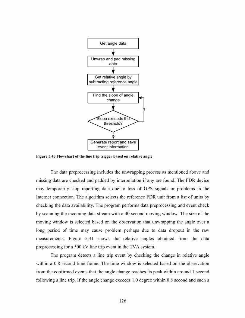
126
Get angle data
Unwrap and pad missing data
Get relative angle by subtracting reference angle
Find the slope of angle change
Slope exceeds the threshold?
Generate report and save event information
Y
N
Figure 5.40 Flowchart of the line trip trigger based on relative angle
The data preprocessing includes the unwrapping process as mentioned above and
missing data are checked and padded by interpolation if any are found. The FDR device
may temporarily stop reporting data due to loss of GPS signals or problems in the
Internet connection. The algorithm selects the reference FDR unit from a list of units by
checking the data availability. The program performs data preprocessing and event check
by scanning the incoming data stream with a 40-second moving window. The size of the
moving window is selected based on the observation that unwrapping the angle over a
long period of time may cause problem perhaps due to data dropout in the raw
measurements. Figure 5.41 shows the relative angles obtained from the data
preprocessing for a 500 kV line trip event in the TVA system.
The program detects a line trip event by checking the change in relative angle
within a 0.8-second time frame. The time window is selected based on the observation
from the confirmed events that the angle change reaches its peak within around 1 second
following a line trip. If the angle change exceeds 1.0 degree within 0.8 second and such a
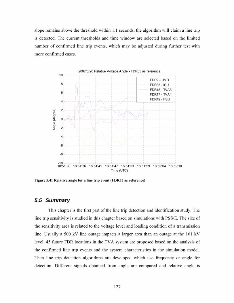
127
slope remains above the threshold within 1.1 seconds, the algorithm will claim a line trip
is detected. The current thresholds and time window are selected based on the limited
number of confirmed line trip events, which may be adjusted during further test with
more confirmed cases.
18:51:30 18:51:36 18:51:41 18:51:47 18:51:53 18:51:59 18:52:04 18:52:10-10
-8
-6
-4
-2
0
2
4
6
8
10
Time (UTC)
Ang
le (d
egre
e)
2007/6/28 Relative Voltage Angle - FDR35 as reference
FDR2 - UMRFDR35 - ISUFDR15 - TVA3FDR17 - TVA4FDR42 - FSU
Figure 5.41 Relative angle for a line trip event (FDR35 as reference)
5.5 Summary
This chapter is the first part of the line trip detection and identification study. The
line trip sensitivity is studied in this chapter based on simulations with PSS/E. The size of
the sensitivity area is related to the voltage level and loading condition of a transmission
line. Usually a 500 kV line outage impacts a larger area than an outage at the 161 kV
level. 45 future FDR locations in the TVA system are proposed based on the analysis of
the confirmed line trip events and the system characteristics in the simulation model.
Then line trip detection algorithms are developed which use frequency or angle for
detection. Different signals obtained from angle are compared and relative angle is

128
selected. The proposed frequency and angle triggers are simple and can both be
implemented fairly easily for real time line trip detection.

129
Chapter 6 Line Trip Identification As a continuation of the study in chapter 5, this chapter focuses on single line trip
identification. The question of interest is which line is tripped if one occurs. The study in
this chapter will employ the simulations with PSS/E extensively based on the Eastern
Interconnection model. The model is comprehensive and detailed which contains voltage
levels from 765 kV to distribution level. There are 2287 generators and 16016 buses in
service in the model. In addition, there are 20093 transmission lines and 7221 branches
with transformers. The system’s total active power generation is 590476.8 MW and the
reactive power generation is 137509.9 MVAR [54]. The simulation will help identifying
the characteristics of line trips.
6.1 Line Trip Characteristics – A Close Examination
The objective of line trip study in this work is to utilize wide-area measurements
provided by FNET to detect a line outage when it occurs and identify the tripped line.
Therefore, it is essential to study the line trip characteristics reflected in the power system
parameters such as frequency and phase angle. In this section, the line trip characteristics
are examined with PSS/E simulation and real frequency and angle measurements.
When a transmission line is tripped, the angular velocity of the machines at the
sending end increases due to the sudden loss of load; while the angular velocity of the
machines at the receiving end deceases [62]. The local phase angle and frequency change
together. Hence the angle also experiences changes due to the line outage. Some
frequency and angle plots of line trip events have been illustrated in Chapter 5. The
information in the measurements for line trip identification will be closely examined as
follows.
6.1.1 Line Trip Signatures in PSS/E Simulation
In the PSS/E model of the Eastern Interconnection used for this study, 70
transmission lines at 500 kV voltage level have been identified in the TVA system,
among which 7 lines carry zero power flow. The PSS/E simulations in this work are
carried out on the 63 lines with real power flow greater than zero. 52 monitoring channels
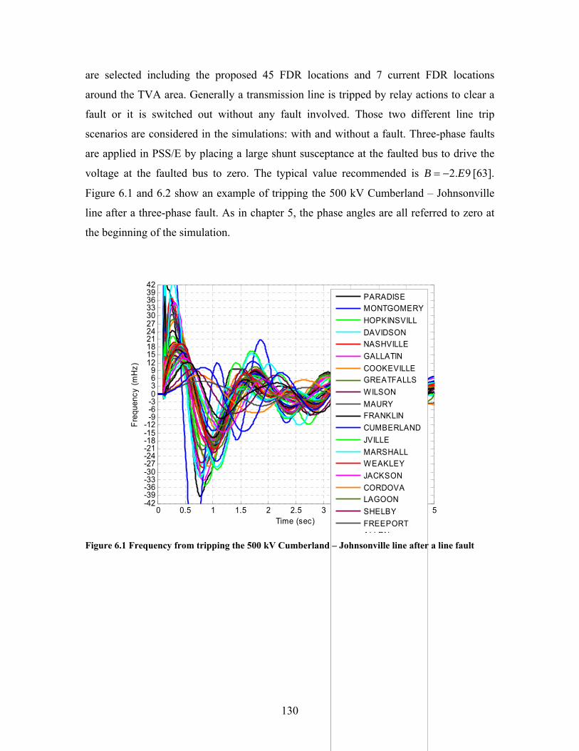
130
are selected including the proposed 45 FDR locations and 7 current FDR locations
around the TVA area. Generally a transmission line is tripped by relay actions to clear a
fault or it is switched out without any fault involved. Those two different line trip
scenarios are considered in the simulations: with and without a fault. Three-phase faults
are applied in PSS/E by placing a large shunt susceptance at the faulted bus to drive the
voltage at the faulted bus to zero. The typical value recommended is 9.2 EB −= [63].
Figure 6.1 and 6.2 show an example of tripping the 500 kV Cumberland – Johnsonville
line after a three-phase fault. As in chapter 5, the phase angles are all referred to zero at
the beginning of the simulation.
0 0.5 1 1.5 2 2.5 3 3.5 4 4.5 5-42-39-36-33-30-27-24-21-18-15-12
-9-6-30369
1215182124273033363942
Time (sec)
Freq
uenc
y (m
Hz)
PARADISEMONTGOMERYHOPKINSVILLDAVIDSONNASHVILLEGALLATINCOOKEVILLEGREATFALLSWILSONMAURYFRANKLINCUMBERLANDJVILLEMARSHALLWEAKLEYJACKSONCORDOVALAGOONSHELBYFREEPORTALLEN
Figure 6.1 Frequency from tripping the 500 kV Cumberland – Johnsonville line after a line fault
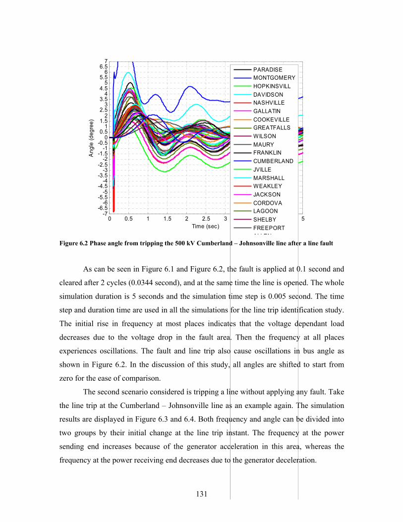
131
0 0.5 1 1.5 2 2.5 3 3.5 4 4.5 5-7
-6.5-6
-5.5-5
-4.5-4
-3.5-3
-2.5-2
-1.5-1
-0.50
0.51
1.52
2.53
3.54
4.55
5.56
6.57
Time (sec)
Ang
le (d
egre
e)
PARADISEMONTGOMERYHOPKINSVILLDAVIDSONNASHVILLEGALLATINCOOKEVILLEGREATFALLSWILSONMAURYFRANKLINCUMBERLANDJVILLEMARSHALLWEAKLEYJACKSONCORDOVALAGOONSHELBYFREEPORTALLEN
Figure 6.2 Phase angle from tripping the 500 kV Cumberland – Johnsonville line after a line fault
As can be seen in Figure 6.1 and Figure 6.2, the fault is applied at 0.1 second and
cleared after 2 cycles (0.0344 second), and at the same time the line is opened. The whole
simulation duration is 5 seconds and the simulation time step is 0.005 second. The time
step and duration time are used in all the simulations for the line trip identification study.
The initial rise in frequency at most places indicates that the voltage dependant load
decreases due to the voltage drop in the fault area. Then the frequency at all places
experiences oscillations. The fault and line trip also cause oscillations in bus angle as
shown in Figure 6.2. In the discussion of this study, all angles are shifted to start from
zero for the ease of comparison.
The second scenario considered is tripping a line without applying any fault. Take
the line trip at the Cumberland – Johnsonville line as an example again. The simulation
results are displayed in Figure 6.3 and 6.4. Both frequency and angle can be divided into
two groups by their initial change at the line trip instant. The frequency at the power
sending end increases because of the generator acceleration in this area, whereas the
frequency at the power receiving end decreases due to the generator deceleration.
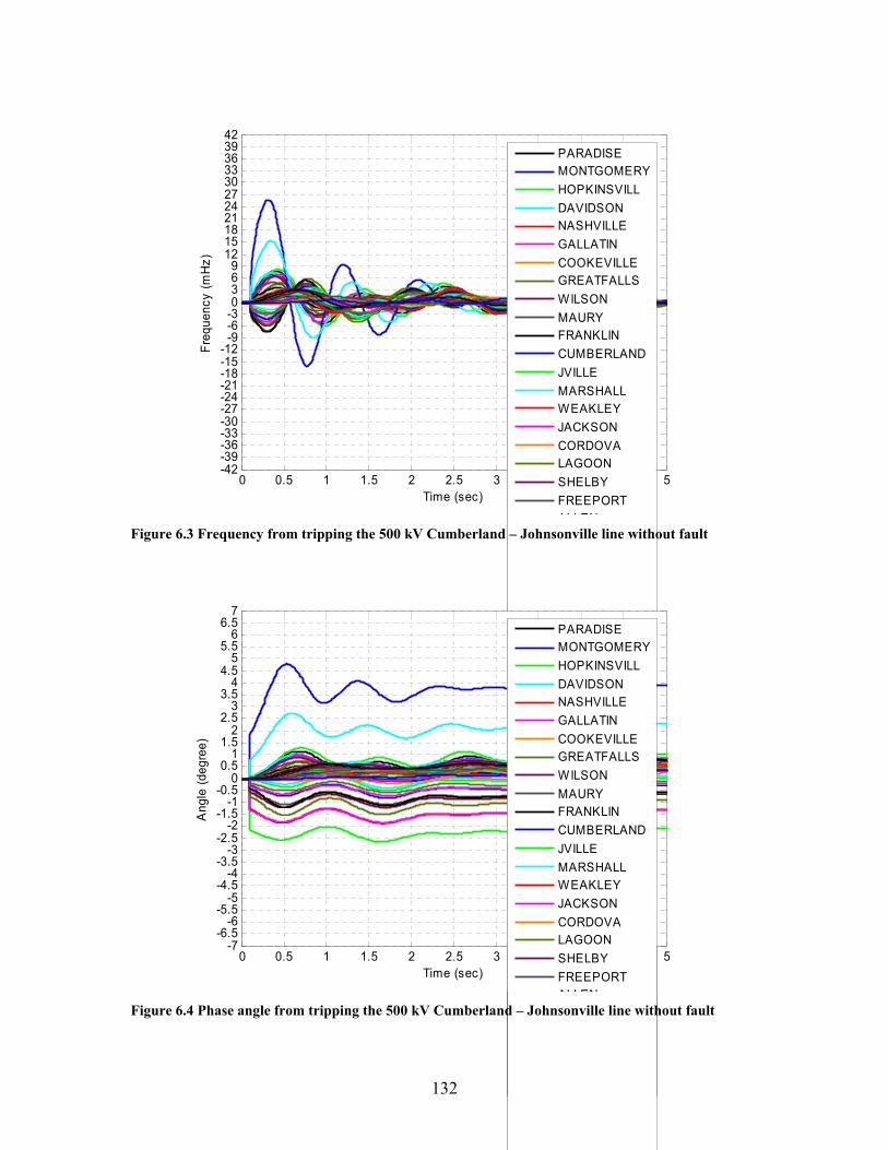
132
0 0.5 1 1.5 2 2.5 3 3.5 4 4.5 5-42-39-36-33-30-27-24-21-18-15-12
-9-6-30369
1215182124273033363942
Time (sec)
Freq
uenc
y (m
Hz)
PARADISEMONTGOMERYHOPKINSVILLDAVIDSONNASHVILLEGALLATINCOOKEVILLEGREATFALLSWILSONMAURYFRANKLINCUMBERLANDJVILLEMARSHALLWEAKLEYJACKSONCORDOVALAGOONSHELBYFREEPORTALLEN
Figure 6.3 Frequency from tripping the 500 kV Cumberland – Johnsonville line without fault
0 0.5 1 1.5 2 2.5 3 3.5 4 4.5 5-7
-6.5-6
-5.5-5
-4.5-4
-3.5-3
-2.5-2
-1.5-1
-0.50
0.51
1.52
2.53
3.54
4.55
5.56
6.57
Time (sec)
Ang
le (d
egre
e)
PARADISEMONTGOMERYHOPKINSVILLDAVIDSONNASHVILLEGALLATINCOOKEVILLEGREATFALLSWILSONMAURYFRANKLINCUMBERLANDJVILLEMARSHALLWEAKLEYJACKSONCORDOVALAGOONSHELBYFREEPORTALLEN
Figure 6.4 Phase angle from tripping the 500 kV Cumberland – Johnsonville line without fault

133
Apparently the magnitudes of frequency and angle oscillations in Figure 6.3 and
Figure 6.4 are much less than in the previous case that involves a line fault. It
demonstrates that a line trip following a fault is generally more severe than only tripping
the line. Therefore, it is reasonable to focus on the scenario of single line trip without a
fault in simulation for line trip detection study because the line trip following a fault
usually causes larger variations in frequency and angle thus easier to detect. From this
point on, this work will develop the line trip identification algorithm based on the
simulation of single line trip without any fault.
Validation tests on the PSS/E simulation results have been conducted to verify
whether the derivative of voltage phase angle agrees with the bus frequency since
frequency can be obtained by taking the derivative of angle. Figure 6.5 and Figure 6.7
show the comparisons between frequency and angle derivative, phase angle and
integrated frequency respectively for tripping the 500 kV Cumberland – Johnsonville
line. The derivative of the phase angle in Figure 6.5 is approximated as the angle
difference between two adjacent points along the time axis as in (6.1). t∆ is the
simulation time step which is 0.005 second in this case.
tdtd
∆∆
≈θθ (6.1)
It is clear in Figure 6.5 that the angle derivative (shown as dotted lines) and the
bus frequency (shown as solid lines) are very close except that there is a large spike in
angle derivative at the instant of the line trip disturbance. It can be noticed in Figure 6.7
that the angle experiences a step change of different size at 0.1 second when the line is
tripped. The large spike in the angle derivative is due to such state change demonstrated
in the angle, which depends on the way that PSS/E deals with dynamic simulation. The
duration of electrical transients may be expected to arise and disappear within a few
milliseconds, while electromechanical transients take several seconds. PSS/E is primarily
concerned with power system dynamic behavior associated with the energy stored in the
rotating inertias of the system, where transients arise and decay away again within a
period of a few seconds [64]. Hence, it is possible that the angle state change due to the
line trip disturbance is treated as a sudden rise or drop at the trip incident. From this
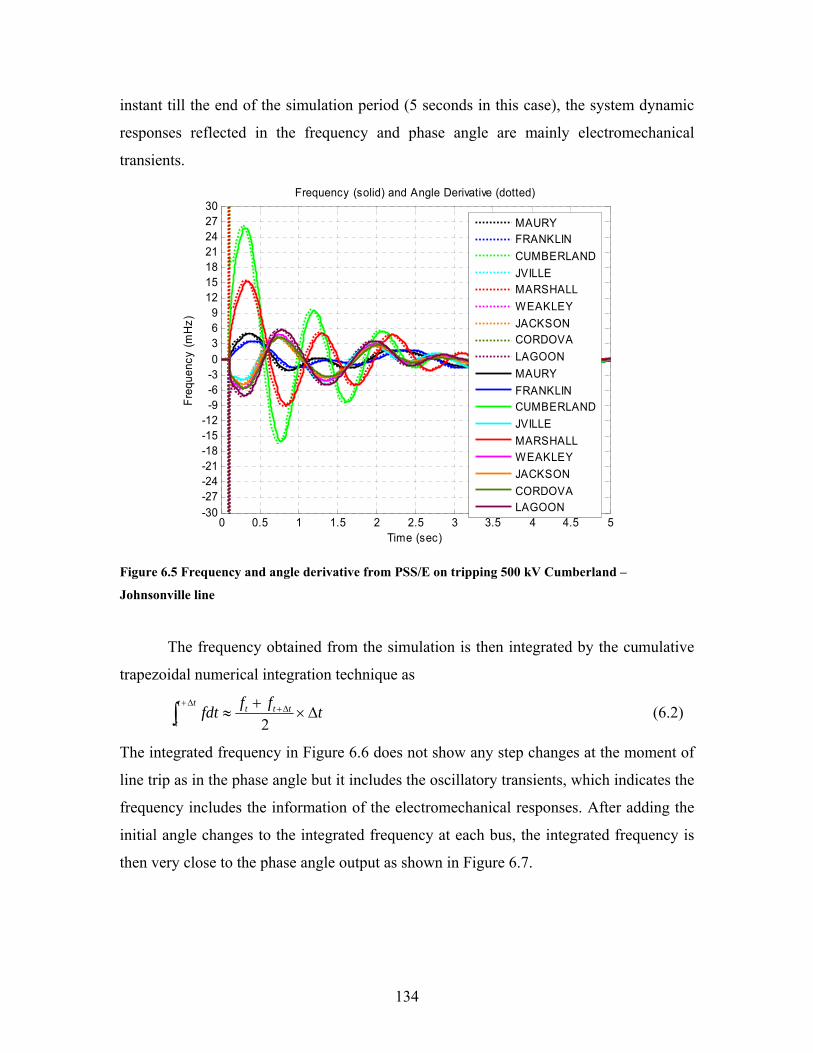
134
instant till the end of the simulation period (5 seconds in this case), the system dynamic
responses reflected in the frequency and phase angle are mainly electromechanical
transients.
0 0.5 1 1.5 2 2.5 3 3.5 4 4.5 5-30-27-24-21-18-15-12
-9-6-30369
12151821242730
Time (sec)
Freq
uenc
y (m
Hz)
Frequency (solid) and Angle Derivative (dotted)
MAURYFRANKLINCUMBERLANDJVILLEMARSHALLWEAKLEYJACKSONCORDOVALAGOONMAURYFRANKLINCUMBERLANDJVILLEMARSHALLWEAKLEYJACKSONCORDOVALAGOON
Figure 6.5 Frequency and angle derivative from PSS/E on tripping 500 kV Cumberland –
Johnsonville line
The frequency obtained from the simulation is then integrated by the cumulative
trapezoidal numerical integration technique as
tfffdt ttttt
t∆×
+≈ ∆+
∆+
∫ 2 (6.2)
The integrated frequency in Figure 6.6 does not show any step changes at the moment of
line trip as in the phase angle but it includes the oscillatory transients, which indicates the
frequency includes the information of the electromechanical responses. After adding the
initial angle changes to the integrated frequency at each bus, the integrated frequency is
then very close to the phase angle output as shown in Figure 6.7.
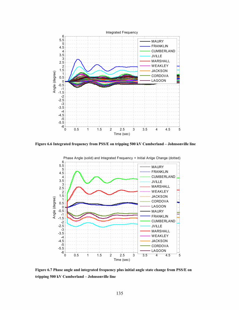
135
0 0.5 1 1.5 2 2.5 3 3.5 4 4.5 5-6
-5.5-5
-4.5-4
-3.5-3
-2.5-2
-1.5-1
-0.50
0.51
1.52
2.53
3.54
4.55
5.56
Ang
le (d
egre
e)
Time (sec)
Integrated Frequency
MAURYFRANKLINCUMBERLANDJVILLEMARSHALLWEAKLEYJACKSONCORDOVALAGOON
Figure 6.6 Integrated frequency from PSS/E on tripping 500 kV Cumberland – Johnsonville line
0 0.5 1 1.5 2 2.5 3 3.5 4 4.5 5-6
-5.5-5
-4.5-4
-3.5-3
-2.5-2
-1.5-1
-0.50
0.51
1.52
2.53
3.54
4.55
5.56
Time (sec)
Ang
le (d
egre
e)
Phase Angle (solid) and Integrated Frequency + Initial Anlge Change (dotted)
MAURYFRANKLINCUMBERLANDJVILLEMARSHALLWEAKLEYJACKSONCORDOVALAGOONMAURYFRANKLINCUMBERLANDJVILLEMARSHALLWEAKLEYJACKSONCORDOVALAGOON
Figure 6.7 Phase angle and integrated frequency plus initial angle state change from PSS/E on
tripping 500 kV Cumberland – Johnsonville line

136
This test also shows that the bus phase angle can be a very useful parameter for
line trip identification. If the DC power flow model is considered, then
∆P = B’ ∆θ (6.3)
ikik x
B 1' −= , assuming a branch from i to k (zero otherwise)
∑=
=N
k ikii x
B1
1'
It can be obtained that
∆θ = B’¹־ ∆P (6.4)
where ∆P is the vector of the changes in bus real power injections, B’ is the bus
susceptance matrix, and ∆θ is the vector of bus angle changes, ikx is the reactance of the
branch from i to k , and N is the number of buses [65]. When a line is tripped, the pre-
outage power flow on the line will be redistributed to other lines in the system, which
causes a change in angles at all buses. That is, the change in angles directly reflects the
effect of a line outage. It is observed that the largest angle changes occur right at the ends
of the tripped line, which may not hold for frequency.
6.1.2 Line Trip Signatures in Real Measurements
As an example, Figure 6.8 and Figure 6.9 show the real measurements form FDRs
for a line outage at the same 500 kV Cumberland – Johnsonville line in the above
simulation case. This 500 kV line trip event occurred at 19:03:19 UTC on April 11, 2007.
The real angle measurements are similar with the simulation results in that the line trip
caused oscillations in frequency and changes in phase angle. The magnitudes of
oscillations resulting from the line trip are different in the simulation and in the real data
due to several possible reasons. One is that in the simulations the monitoring points are
500 kV buses, whereas the FNET data are taken from the distribution network. The
difference is expected also because the simulation model is an approximation of the real
complicated system.
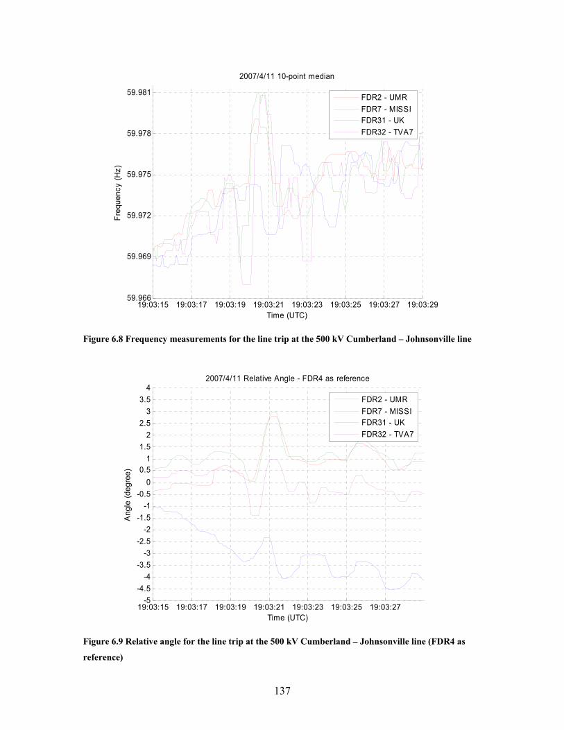
137
19:03:15 19:03:17 19:03:19 19:03:21 19:03:23 19:03:25 19:03:27 19:03:2959.966
59.969
59.972
59.975
59.978
59.981
Time (UTC)
Freq
uenc
y (H
z)
2007/4/11 10-point median
FDR2 - UMRFDR7 - MISSIFDR31 - UKFDR32 - TVA7
Figure 6.8 Frequency measurements for the line trip at the 500 kV Cumberland – Johnsonville line
19:03:15 19:03:17 19:03:19 19:03:21 19:03:23 19:03:25 19:03:27-5
-4.5-4
-3.5-3
-2.5-2
-1.5-1
-0.50
0.51
1.52
2.53
3.54
Time (UTC)
Ang
le (d
egre
e)
2007/4/11 Relative Angle - FDR4 as reference
FDR2 - UMRFDR7 - MISSIFDR31 - UKFDR32 - TVA7
Figure 6.9 Relative angle for the line trip at the 500 kV Cumberland – Johnsonville line (FDR4 as
reference)
138
Another noticeable difference is that the phase angle in the simulation experiences
a sharp step change at the line trip instant, while no such change has been observed in the
real measurements. The FDRs’ output data rate is 10 samples per second hence not
targeting the detection of fast electromagnetic transients within several milliseconds.
However, the information of the electromechanical transients resulting from the
disturbances is well-represented in the measurements.
It has been discussed that the phase angle change directly reflects the power flow
transfer in the transmission lines after a line outage. Thus the phase angle measurements
can be utilized as detection signals for the purpose of line trip identification.
6.2 500 kV and 161 kV Line Trip Detection
As is shown in Figure 6.5, the transmission network in the TVA area is mostly
composed by two voltage levels: 500 kV and 161 kV. The impact of a 500 kV line trip is
generally larger than the outage at a 161 kV line since a 500 kV line usually carries more
power than a 161 kV line.
6.2.1 500 kV Line Trip Detection Simulation Study
The 63 identified 500 kV transmission lines are tripped one at a time with PSS/E.
The frequency and angle at the 52 selected buses are monitored. All the simulation results
are similar as in Figure 6.3 and Figure 6.4 although the magnitudes of frequency
oscillations and angle changes may be different.
The power flow directions in the 500 kV transmission network are also examined
in PSS/E in order to study the power transfer in the system (Figure 5.22). For the
transmission corridor in the east of the TVA system, the power flow in PSS/E simulation
follows the direction from south to north because there are several nuclear and hydro
power plants such as Watts Bar and Sequoyah in the south part of Tennessee, thus power
is transferred from the generation source to the load area. If, for example, the sensors
located close to this corridor detect angle changes that are out of phase, it can be decided
that the tripped line is along this transmission corridor. The locations of the sensors can
help to decide at which section of the transmission corridor the line is tripped. However,
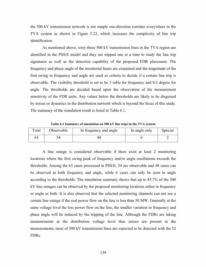
139
the 500 kV transmission network is not simple one-direction corridor everywhere in the
TVA system as shown in Figure 5.22, which increases the complexity of line trip
identification.
As mentioned above, sixty-three 500 kV transmission lines in the TVA region are
identified in the PSS/E model and they are tripped one at a time to study the line trip
signatures as well as the detection capability of the proposed FDR placement. The
frequency and phase angle of the monitored buses are examined and the magnitude of the
first swing in frequency and angle are used as criteria to decide if a certain line trip is
observable. The visibility threshold is set to be 3 mHz for frequency and 0.5 degree for
angle. The thresholds are decided based upon the observation of the measurement
sensitivity of the FDR units. Any values below the thresholds are likely to be disguised
by noises or dynamics in the distribution network which is beyond the focus of this study.
The summary of the simulation result is listed in Table 6.1.
Table 6.1 Summary of simulation on 500 kV line trips in the TVA system
Total Observable In frequency and angle In angle only Special
63 54 48 6 2
A line outage is considered observable if there exist at least 2 monitoring
locations where the first swing peak of frequency and/or angle oscillations exceeds the
thresholds. Among the 63 cases processed in PSS/E, 54 are observable and 48 cases can
be observed in both frequency and angle, while 6 cases can only be seen in angle
according to the thresholds. The simulation summary shows that up to 85.7% of the 500
kV line outages can be observed by the proposed monitoring locations either in frequency
or angle or both. It is also observed that the selected monitoring channels can not see a
certain line outage if the real power flow on the line is less than 50 MW. Generally at the
same voltage level the less power flow on the line, the smaller variation in frequency and
phase angle will be induced by the tripping of the line. Although the FDRs are taking
measurements at the distribution voltage level thus noises are present in the
measurements, most of 500 kV transmission lines are expected to be detected with the 52
FDRs.
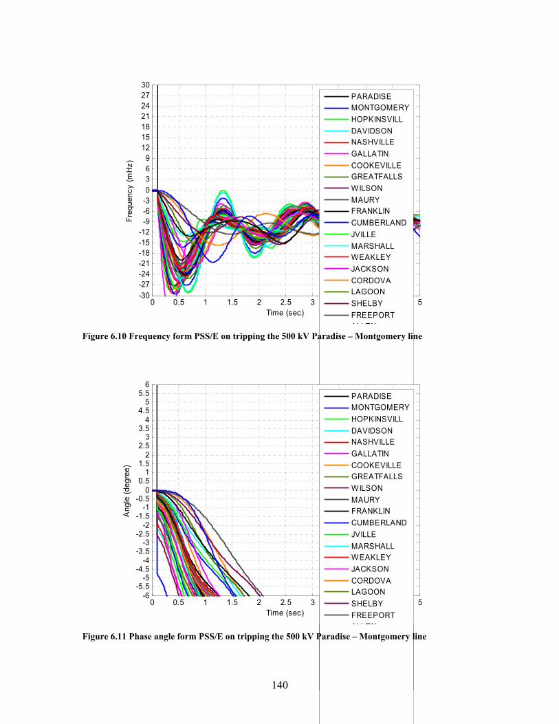
140
0 0.5 1 1.5 2 2.5 3 3.5 4 4.5 5-30-27-24-21-18-15-12
-9-6-30369
12151821242730
Time (sec)
Freq
uenc
y (m
Hz)
PARADISEMONTGOMERYHOPKINSVILLDAVIDSONNASHVILLEGALLATINCOOKEVILLEGREATFALLSWILSONMAURYFRANKLINCUMBERLANDJVILLEMARSHALLWEAKLEYJACKSONCORDOVALAGOONSHELBYFREEPORTALLEN
Figure 6.10 Frequency form PSS/E on tripping the 500 kV Paradise – Montgomery line
0 0.5 1 1.5 2 2.5 3 3.5 4 4.5 5-6
-5.5-5
-4.5-4
-3.5-3
-2.5-2
-1.5-1
-0.50
0.51
1.52
2.53
3.54
4.55
5.56
Time (sec)
Ang
le (d
egre
e)
PARADISEMONTGOMERYHOPKINSVILLDAVIDSONNASHVILLEGALLATINCOOKEVILLEGREATFALLSWILSONMAURYFRANKLINCUMBERLANDJVILLEMARSHALLWEAKLEYJACKSONCORDOVALAGOONSHELBYFREEPORTALLEN
Figure 6.11 Phase angle form PSS/E on tripping the 500 kV Paradise – Montgomery line
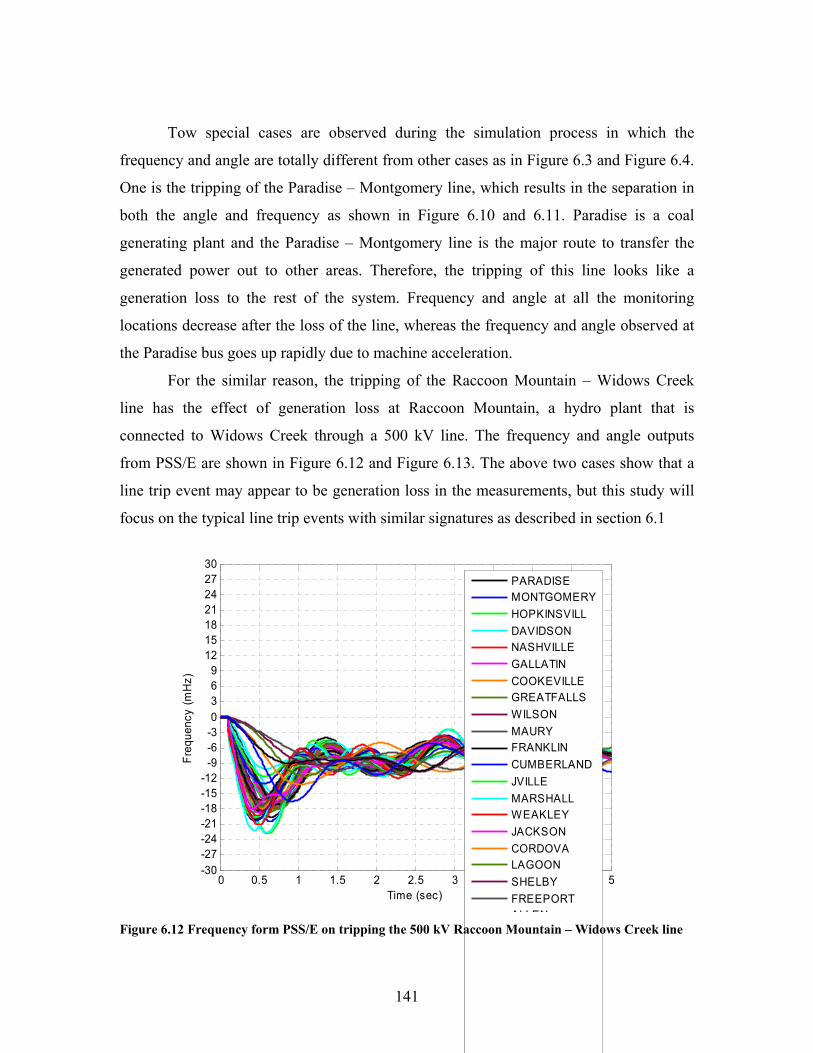
141
Tow special cases are observed during the simulation process in which the
frequency and angle are totally different from other cases as in Figure 6.3 and Figure 6.4.
One is the tripping of the Paradise – Montgomery line, which results in the separation in
both the angle and frequency as shown in Figure 6.10 and 6.11. Paradise is a coal
generating plant and the Paradise – Montgomery line is the major route to transfer the
generated power out to other areas. Therefore, the tripping of this line looks like a
generation loss to the rest of the system. Frequency and angle at all the monitoring
locations decrease after the loss of the line, whereas the frequency and angle observed at
the Paradise bus goes up rapidly due to machine acceleration.
For the similar reason, the tripping of the Raccoon Mountain – Widows Creek
line has the effect of generation loss at Raccoon Mountain, a hydro plant that is
connected to Widows Creek through a 500 kV line. The frequency and angle outputs
from PSS/E are shown in Figure 6.12 and Figure 6.13. The above two cases show that a
line trip event may appear to be generation loss in the measurements, but this study will
focus on the typical line trip events with similar signatures as described in section 6.1
0 0.5 1 1.5 2 2.5 3 3.5 4 4.5 5-30-27-24-21-18-15-12
-9-6-30369
12151821242730
Time (sec)
Freq
uenc
y (m
Hz)
PARADISEMONTGOMERYHOPKINSVILLDAVIDSONNASHVILLEGALLATINCOOKEVILLEGREATFALLSWILSONMAURYFRANKLINCUMBERLANDJVILLEMARSHALLWEAKLEYJACKSONCORDOVALAGOONSHELBYFREEPORTALLEN
Figure 6.12 Frequency form PSS/E on tripping the 500 kV Raccoon Mountain – Widows Creek line
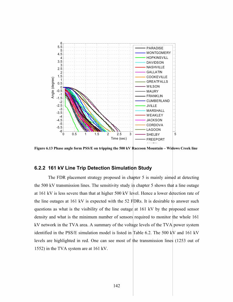
142
0 0.5 1 1.5 2 2.5 3 3.5 4 4.5 5-6
-5.5-5
-4.5-4
-3.5-3
-2.5-2
-1.5-1
-0.50
0.51
1.52
2.53
3.54
4.55
5.56
Time (sec)
Ang
le (d
egre
e)PARADISEMONTGOMERYHOPKINSVILLDAVIDSONNASHVILLEGALLATINCOOKEVILLEGREATFALLSWILSONMAURYFRANKLINCUMBERLANDJVILLEMARSHALLWEAKLEYJACKSONCORDOVALAGOONSHELBYFREEPORTALLEN
Figure 6.13 Phase angle form PSS/E on tripping the 500 kV Raccoon Mountain – Widows Creek line
6.2.2 161 kV Line Trip Detection Simulation Study
The FDR placement strategy proposed in chapter 5 is mainly aimed at detecting
the 500 kV transmission lines. The sensitivity study in chapter 5 shows that a line outage
at 161 kV is less severe than that at higher 500 kV level. Hence a lower detection rate of
the line outages at 161 kV is expected with the 52 FDRs. It is desirable to answer such
questions as what is the visibility of the line outage at 161 kV by the proposed sensor
density and what is the minimum number of sensors required to monitor the whole 161
kV network in the TVA area. A summary of the voltage levels of the TVA power system
identified in the PSS/E simulation model is listed in Table 6.2. The 500 kV and 161 kV
levels are highlighted in red. One can see most of the transmission lines (1253 out of
1552) in the TVA system are at 161 kV.
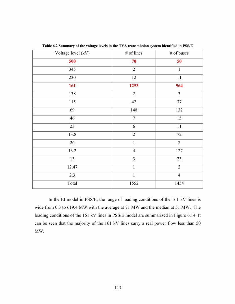
143
Table 6.2 Summary of the voltage levels in the TVA transmission system identified in PSS/E
Voltage level (kV) # of lines # of buses
500 70 50
345 2 1
230 12 11
161 1253 964
138 2 3
115 42 37
69 148 132
46 7 15
23 6 11
13.8 2 72
26 1 2
13.2 4 127
13 3 23
12.47 1 2
2.3 1 4
Total 1552 1454
In the EI model in PSS/E, the range of loading conditions of the 161 kV lines is
wide from 0.3 to 619.4 MW with the average at 71 MW and the median at 51 MW. The
loading conditions of the 161 kV lines in PSS/E model are summarized in Figure 6.14. It
can be seen that the majority of the 161 kV lines carry a real power flow less than 50
MW.
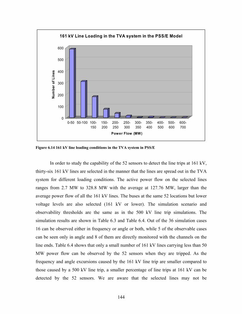
144
0
100
200
300
400
500
600N
umbe
r of
Lin
es
0-50 50-100 100-150
150-200
200-250
250-300
300-350
350-400
400-500
500-600
600-700
Power Flow (MW)
161 kV Line Loading in the TVA system in the PSS/E Model
Figure 6.14 161 kV line loading conditions in the TVA system in PSS/E
In order to study the capability of the 52 sensors to detect the line trips at 161 kV,
thirty-six 161 kV lines are selected in the manner that the lines are spread out in the TVA
system for different loading conditions. The active power flow on the selected lines
ranges from 2.7 MW to 328.8 MW with the average at 127.76 MW, larger than the
average power flow of all the 161 kV lines. The buses at the same 52 locations but lower
voltage levels are also selected (161 kV or lower). The simulation scenario and
observability thresholds are the same as in the 500 kV line trip simulations. The
simulation results are shown in Table 6.3 and Table 6.4. Out of the 36 simulation cases
16 can be observed either in frequency or angle or both, while 5 of the observable cases
can be seen only in angle and 8 of them are directly monitored with the channels on the
line ends. Table 6.4 shows that only a small number of 161 kV lines carrying less than 50
MW power flow can be observed by the 52 sensors when they are tripped. As the
frequency and angle excursions caused by the 161 kV line trip are smaller compared to
those caused by a 500 kV line trip, a smaller percentage of line trips at 161 kV can be
detected by the 52 sensors. We are aware that the selected lines may not be
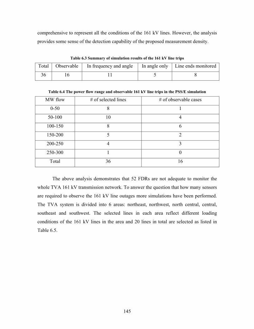
145
comprehensive to represent all the conditions of the 161 kV lines. However, the analysis
provides some sense of the detection capability of the proposed measurement density.
Table 6.3 Summary of simulation results of the 161 kV line trips
Total Observable In frequency and angle In angle only Line ends monitored
36 16 11 5 8
Table 6.4 The power flow range and observable 161 kV line trips in the PSS/E simulation
MW flow # of selected lines # of observable cases
0-50 8 1
50-100 10 4
100-150 8 6
150-200 5 2
200-250 4 3
250-300 1 0
Total 36 16
The above analysis demonstrates that 52 FDRs are not adequate to monitor the
whole TVA 161 kV transmission network. To answer the question that how many sensors
are required to observe the 161 kV line outages more simulations have been performed.
The TVA system is divided into 6 areas: northeast, northwest, north central, central,
southeast and southwest. The selected lines in each area reflect different loading
conditions of the 161 kV lines in the area and 20 lines in total are selected as listed in
Table 6.5.
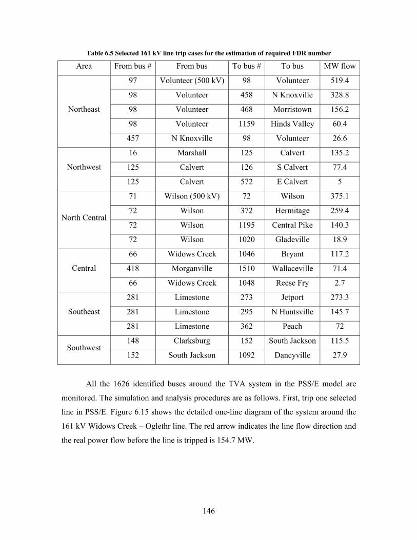
146
Table 6.5 Selected 161 kV line trip cases for the estimation of required FDR number
Area From bus # From bus To bus # To bus MW flow
97 Volunteer (500 kV) 98 Volunteer 519.4
98 Volunteer 458 N Knoxville 328.8
98 Volunteer 468 Morristown 156.2
98 Volunteer 1159 Hinds Valley 60.4
Northeast
457 N Knoxville 98 Volunteer 26.6
16 Marshall 125 Calvert 135.2
125 Calvert 126 S Calvert 77.4 Northwest
125 Calvert 572 E Calvert 5
71 Wilson (500 kV) 72 Wilson 375.1
72 Wilson 372 Hermitage 259.4
72 Wilson 1195 Central Pike 140.3 North Central
72 Wilson 1020 Gladeville 18.9
66 Widows Creek 1046 Bryant 117.2
418 Morganville 1510 Wallaceville 71.4 Central
66 Widows Creek 1048 Reese Fry 2.7
281 Limestone 273 Jetport 273.3
281 Limestone 295 N Huntsville 145.7 Southeast
281 Limestone 362 Peach 72
148 Clarksburg 152 South Jackson 115.5 Southwest
152 South Jackson 1092 Dancyville 27.9
All the 1626 identified buses around the TVA system in the PSS/E model are
monitored. The simulation and analysis procedures are as follows. First, trip one selected
line in PSS/E. Figure 6.15 shows the detailed one-line diagram of the system around the
161 kV Widows Creek – Oglethr line. The red arrow indicates the line flow direction and
the real power flow before the line is tripped is 154.7 MW.
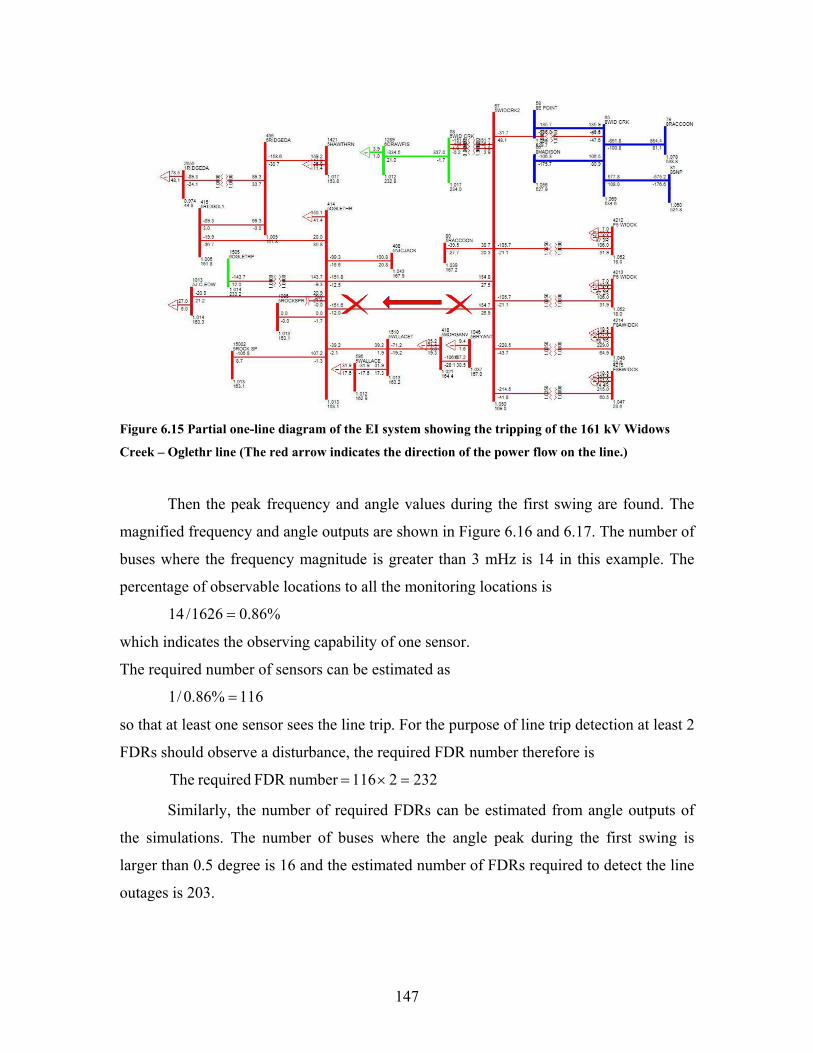
147
Figure 6.15 Partial one-line diagram of the EI system showing the tripping of the 161 kV Widows
Creek – Oglethr line (The red arrow indicates the direction of the power flow on the line.)
Then the peak frequency and angle values during the first swing are found. The
magnified frequency and angle outputs are shown in Figure 6.16 and 6.17. The number of
buses where the frequency magnitude is greater than 3 mHz is 14 in this example. The
percentage of observable locations to all the monitoring locations is
%86.01626/14 =
which indicates the observing capability of one sensor.
The required number of sensors can be estimated as
116%86.0/1 =
so that at least one sensor sees the line trip. For the purpose of line trip detection at least 2
FDRs should observe a disturbance, the required FDR number therefore is
2322116number FDR required The =×=
Similarly, the number of required FDRs can be estimated from angle outputs of
the simulations. The number of buses where the angle peak during the first swing is
larger than 0.5 degree is 16 and the estimated number of FDRs required to detect the line
outages is 203.
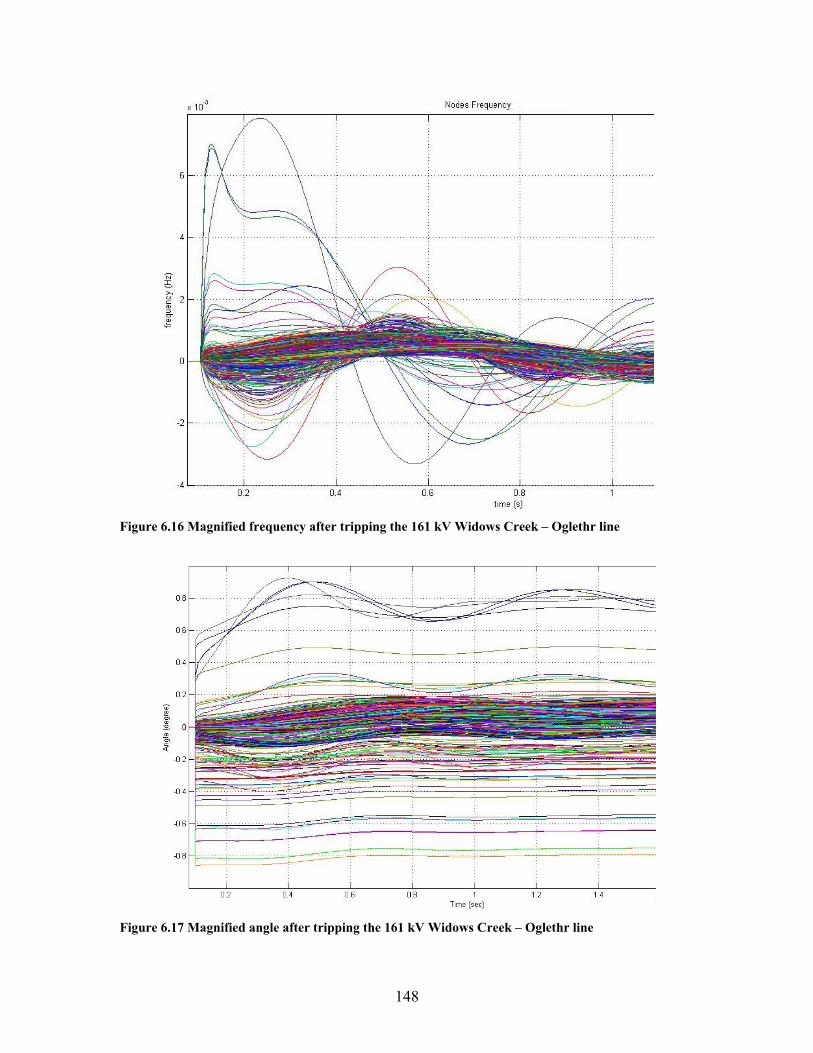
148
Figure 6.16 Magnified frequency after tripping the 161 kV Widows Creek – Oglethr line
Figure 6.17 Magnified angle after tripping the 161 kV Widows Creek – Oglethr line
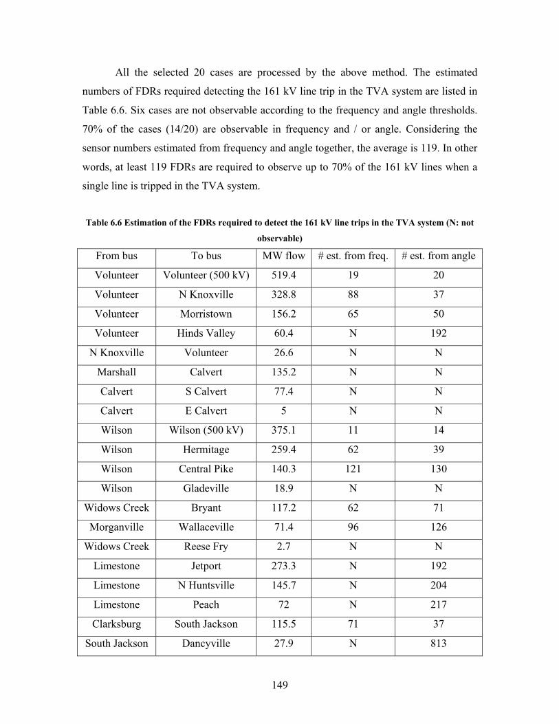
149
All the selected 20 cases are processed by the above method. The estimated
numbers of FDRs required detecting the 161 kV line trip in the TVA system are listed in
Table 6.6. Six cases are not observable according to the frequency and angle thresholds.
70% of the cases (14/20) are observable in frequency and / or angle. Considering the
sensor numbers estimated from frequency and angle together, the average is 119. In other
words, at least 119 FDRs are required to observe up to 70% of the 161 kV lines when a
single line is tripped in the TVA system.
Table 6.6 Estimation of the FDRs required to detect the 161 kV line trips in the TVA system (N: not
observable)
From bus To bus MW flow # est. from freq. # est. from angle
Volunteer Volunteer (500 kV) 519.4 19 20
Volunteer N Knoxville 328.8 88 37
Volunteer Morristown 156.2 65 50
Volunteer Hinds Valley 60.4 N 192
N Knoxville Volunteer 26.6 N N
Marshall Calvert 135.2 N N
Calvert S Calvert 77.4 N N
Calvert E Calvert 5 N N
Wilson Wilson (500 kV) 375.1 11 14
Wilson Hermitage 259.4 62 39
Wilson Central Pike 140.3 121 130
Wilson Gladeville 18.9 N N
Widows Creek Bryant 117.2 62 71
Morganville Wallaceville 71.4 96 126
Widows Creek Reese Fry 2.7 N N
Limestone Jetport 273.3 N 192
Limestone N Huntsville 145.7 N 204
Limestone Peach 72 N 217
Clarksburg South Jackson 115.5 71 37
South Jackson Dancyville 27.9 N 813
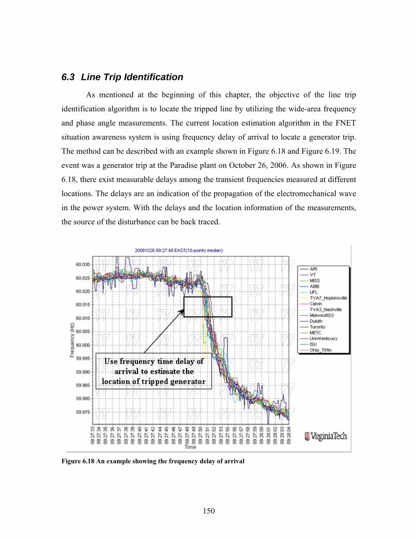
150
6.3 Line Trip Identification
As mentioned at the beginning of this chapter, the objective of the line trip
identification algorithm is to locate the tripped line by utilizing the wide-area frequency
and phase angle measurements. The current location estimation algorithm in the FNET
situation awareness system is using frequency delay of arrival to locate a generator trip.
The method can be described with an example shown in Figure 6.18 and Figure 6.19. The
event was a generator trip at the Paradise plant on October 26, 2006. As shown in Figure
6.18, there exist measurable delays among the transient frequencies measured at different
locations. The delays are an indication of the propagation of the electromechanical wave
in the power system. With the delays and the location information of the measurements,
the source of the disturbance can be back traced.
Figure 6.18 An example showing the frequency delay of arrival
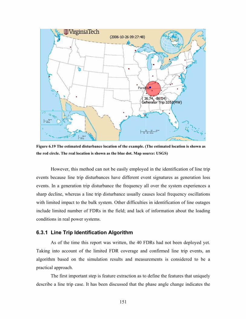
151
Figure 6.19 The estimated disturbance location of the example. (The estimated location is shown as
the red circle. The real location is shown as the blue dot. Map source: USGS)
However, this method can not be easily employed in the identification of line trip
events because line trip disturbances have different event signatures as generation loss
events. In a generation trip disturbance the frequency all over the system experiences a
sharp decline, whereas a line trip disturbance usually causes local frequency oscillations
with limited impact to the bulk system. Other difficulties in identification of line outages
include limited number of FDRs in the field; and lack of information about the loading
conditions in real power systems.
6.3.1 Line Trip Identification Algorithm
As of the time this report was written, the 40 FDRs had not been deployed yet.
Taking into account of the limited FDR coverage and confirmed line trip events, an
algorithm based on the simulation results and measurements is considered to be a
practical approach.
The first important step is feature extraction as to define the features that uniquely
describe a line trip case. It has been discussed that the phase angle change indicates the
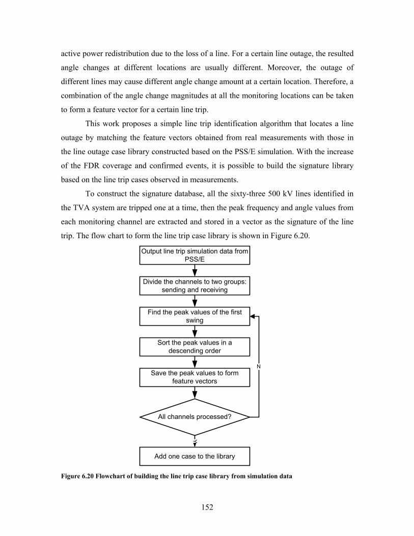
152
active power redistribution due to the loss of a line. For a certain line outage, the resulted
angle changes at different locations are usually different. Moreover, the outage of
different lines may cause different angle change amount at a certain location. Therefore, a
combination of the angle change magnitudes at all the monitoring locations can be taken
to form a feature vector for a certain line trip.
This work proposes a simple line trip identification algorithm that locates a line
outage by matching the feature vectors obtained from real measurements with those in
the line outage case library constructed based on the PSS/E simulation. With the increase
of the FDR coverage and confirmed events, it is possible to build the signature library
based on the line trip cases observed in measurements.
To construct the signature database, all the sixty-three 500 kV lines identified in
the TVA system are tripped one at a time, then the peak frequency and angle values from
each monitoring channel are extracted and stored in a vector as the signature of the line
trip. The flow chart to form the line trip case library is shown in Figure 6.20.
Output line trip simulation data from PSS/E
Divide the channels to two groups: sending and receiving
Find the peak values of the first swing
Sort the peak values in a descending order
All channels processed?
Add one case to the library
Y
NSave the peak values to form
feature vectors
Figure 6.20 Flowchart of building the line trip case library from simulation data
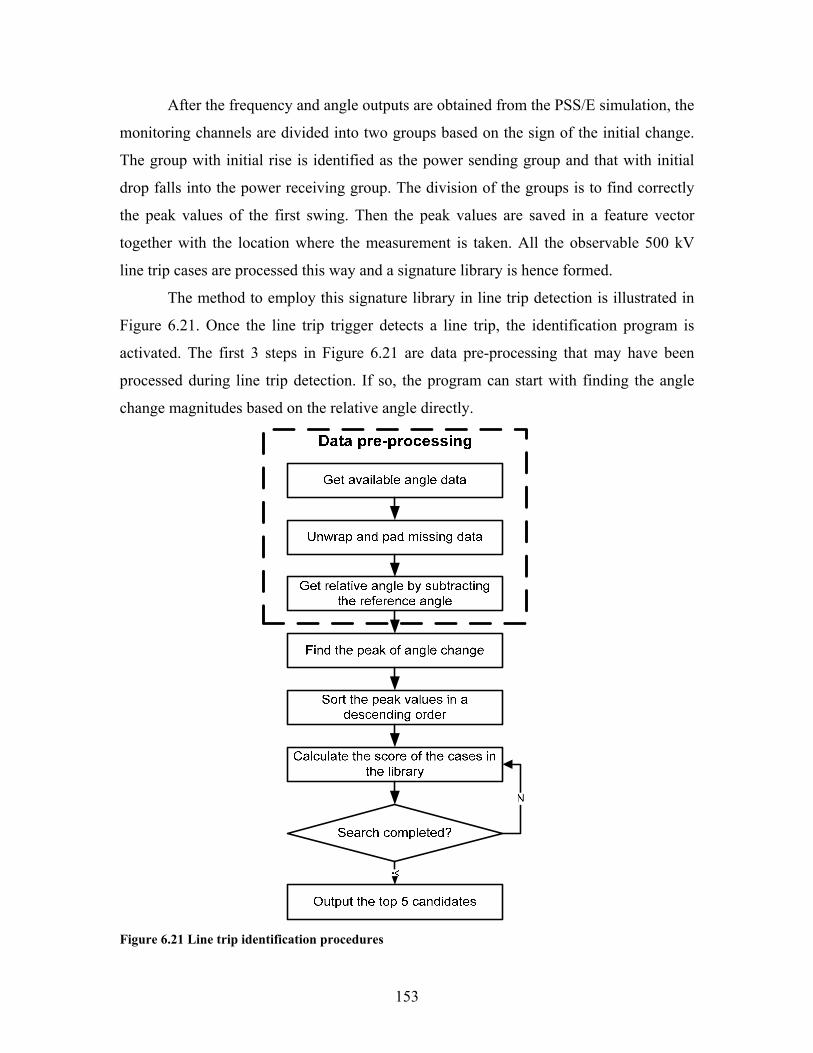
153
After the frequency and angle outputs are obtained from the PSS/E simulation, the
monitoring channels are divided into two groups based on the sign of the initial change.
The group with initial rise is identified as the power sending group and that with initial
drop falls into the power receiving group. The division of the groups is to find correctly
the peak values of the first swing. Then the peak values are saved in a feature vector
together with the location where the measurement is taken. All the observable 500 kV
line trip cases are processed this way and a signature library is hence formed.
The method to employ this signature library in line trip detection is illustrated in
Figure 6.21. Once the line trip trigger detects a line trip, the identification program is
activated. The first 3 steps in Figure 6.21 are data pre-processing that may have been
processed during line trip detection. If so, the program can start with finding the angle
change magnitudes based on the relative angle directly.
Figure 6.21 Line trip identification procedures
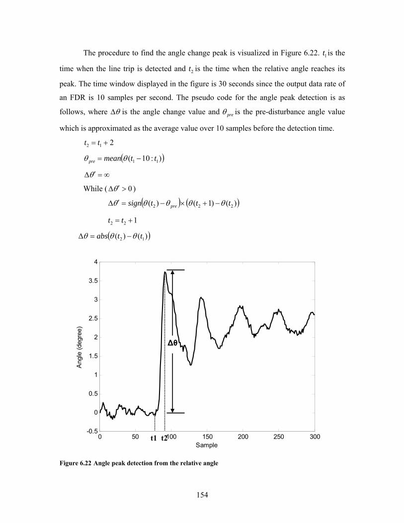
154
The procedure to find the angle change peak is visualized in Figure 6.22. 1t is the
time when the line trip is detected and 2t is the time when the relative angle reaches its
peak. The time window displayed in the figure is 30 seconds since the output data rate of
an FDR is 10 samples per second. The pseudo code for the angle peak detection is as
follows, where θ∆ is the angle change value and preθ is the pre-disturbance angle value
which is approximated as the average value over 10 samples before the detection time.
212 += tt
( )):10( 11 ttmeanpre −= θθ
∞=′∆θ
While ( 0>′∆θ )
( ) ( ))()1()( 222 tttsign pre θθθθθ −+×−=′∆
122 += tt
( ))()( 12 ttabs θθθ −=∆
0 50 100 150 200 250 300-0.5
0
0.5
1
1.5
2
2.5
3
3.5
4
Ang
le (d
egre
e)
Sample
Figure 6.22 Angle peak detection from the relative angle
∆θ
t1 t2

155
Once the angle change peak value θ∆ is found for each available FDR, an
observed feature vector is formed in which the angle peak values are sorted in a high to
low order in the same format as the signature library. In some instances not all FDRs are
reporting valid data during a certain event. Therefore the program selects only the
corresponding channels in the signature library for comparison.
At lease one criterion is required to describe how close an observed line trip
disturbance matches those in the signature library. In this work, the normalized Euclidean
distance (ED) is used for this purpose [66]. The ED is selected because its computation is
simple and the computation time is currently not an issue as the size of observation
feature vectors is small due to the limited number of available FDRs for a single line trip
incident. For an observed feature vector observedθ∆ of a line trip disturbance
[ ]Tobservednobservedobserved ,,1 θθθ ∆∆=∆ K (6.5)
where n is the number of available FDRs during the event, the corresponding signature
vector libraryθ∆ from the case library is
[ ]Tlibrarynlibrarylibrary ,,1 θθθ ∆∆=∆ K (6.6)
Normalize the vectors by dividing by their norms
[ ]
[ ]library
Tlibrarynlibrary
Nlibrary
observed
Tobservednobserved
Nobserved
θθθθ
θθθθ
∆∆∆
=∆
∆∆∆=∆
−
−
,,1
,,1
K
K
The two vectors represent two points in the Dn − space, nNlibraryNobserved ℜ∈∆∆ −− θθ , . The
ED between the two points to the signature vector of the case l in the database is then
calculated by
( ) ( )2,,2
,1,1 NlibrarynNobservednNlibraryNobservedld −−−− ∆−∆++∆−∆= θθθθ K (6.7)
The EDs are ranking criteria that quantify the closeness of an observed tripped
line to the line outage cases in the database. Hence the best match is the case with the
smallest ED value. The program then report 5 cases with the least EDs as the top five
candidates of the possible lines.
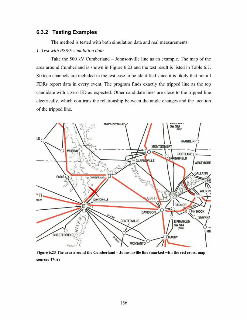
156
6.3.2 Testing Examples
The method is tested with both simulation data and real measurements.
1. Test with PSS/E simulation data
Take the 500 kV Cumberland – Johnsonville line as an example. The map of the
area around Cumberland is shown in Figure 6.23 and the test result is listed in Table 6.7.
Sixteen channels are included in the test case to be identified since it is likely that not all
FDRs report data in every event. The program finds exactly the tripped line as the top
candidate with a zero ED as expected. Other candidate lines are close to the tripped line
electrically, which confirms the relationship between the angle changes and the location
of the tripped line.
Figure 6.23 The area around the Cumberland – Johnsonville line (marked with the red cross. map
source: TVA)
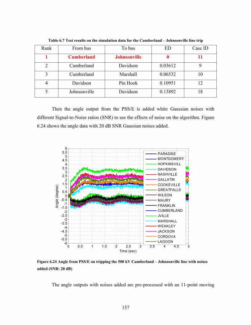
157
Table 6.7 Test results on the simulation data for the Cumberland – Johnsonville line trip
Rank From bus To bus ED Case ID
1 Cumberland Johnsonville 0 11
2 Cumberland Davidson 0.03612 9
3 Cumberland Marshall 0.06532 10
4 Davidson Pin Hook 0.10951 12
5 Johnsonville Davidson 0.13892 18
Then the angle output from the PSS/E is added white Gaussian noises with
different Signal-to-Noise ratios (SNR) to see the effects of noise on the algorithm. Figure
6.24 shows the angle data with 20 dB SNR Gaussian noises added.
0 0.5 1 1.5 2 2.5 3 3.5 4 4.5 5-6
-5.5-5
-4.5-4
-3.5-3
-2.5-2
-1.5-1
-0.50
0.51
1.52
2.53
3.54
4.55
5.56
Time (sec)
Ang
le (d
egre
e)
PARADISEMONTGOMERYHOPKINSVILLDAVIDSONNASHVILLEGALLATINCOOKEVILLEGREATFALLSWILSONMAURYFRANKLINCUMBERLANDJVILLEMARSHALLWEAKLEYJACKSONCORDOVALAGOON
Figure 6.24 Angle from PSS/E on tripping the 500 kV Cumberland – Johnsonville line with noises
added (SNR: 20 dB)
The angle outputs with noises added are pre-processed with an 11-point moving
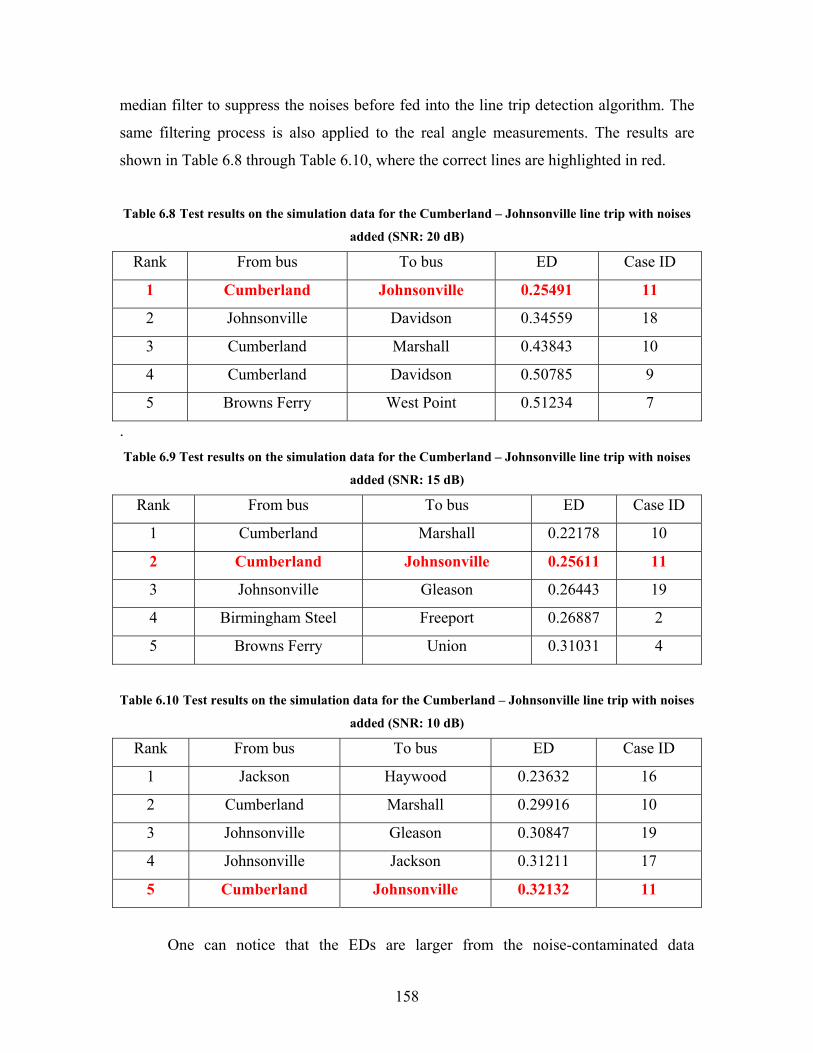
158
median filter to suppress the noises before fed into the line trip detection algorithm. The
same filtering process is also applied to the real angle measurements. The results are
shown in Table 6.8 through Table 6.10, where the correct lines are highlighted in red.
Table 6.8 Test results on the simulation data for the Cumberland – Johnsonville line trip with noises
added (SNR: 20 dB) Rank From bus To bus ED Case ID
1 Cumberland Johnsonville 0.25491 11
2 Johnsonville Davidson 0.34559 18
3 Cumberland Marshall 0.43843 10
4 Cumberland Davidson 0.50785 9
5 Browns Ferry West Point 0.51234 7
. Table 6.9 Test results on the simulation data for the Cumberland – Johnsonville line trip with noises
added (SNR: 15 dB)
Rank From bus To bus ED Case ID
1 Cumberland Marshall 0.22178 10
2 Cumberland Johnsonville 0.25611 11
3 Johnsonville Gleason 0.26443 19
4 Birmingham Steel Freeport 0.26887 2
5 Browns Ferry Union 0.31031 4
Table 6.10 Test results on the simulation data for the Cumberland – Johnsonville line trip with noises
added (SNR: 10 dB) Rank From bus To bus ED Case ID
1 Jackson Haywood 0.23632 16
2 Cumberland Marshall 0.29916 10
3 Johnsonville Gleason 0.30847 19
4 Johnsonville Jackson 0.31211 17
5 Cumberland Johnsonville 0.32132 11
One can notice that the EDs are larger from the noise-contaminated data
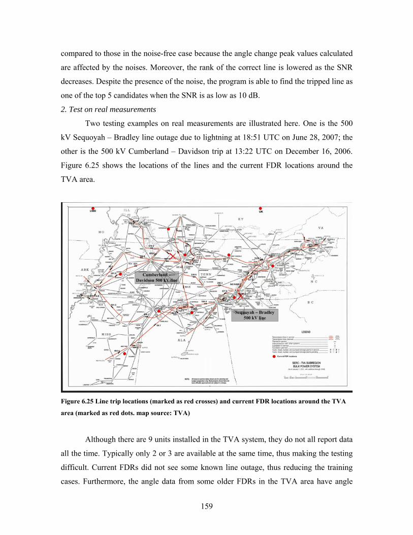
159
compared to those in the noise-free case because the angle change peak values calculated
are affected by the noises. Moreover, the rank of the correct line is lowered as the SNR
decreases. Despite the presence of the noise, the program is able to find the tripped line as
one of the top 5 candidates when the SNR is as low as 10 dB.
2. Test on real measurements
Two testing examples on real measurements are illustrated here. One is the 500
kV Sequoyah – Bradley line outage due to lightning at 18:51 UTC on June 28, 2007; the
other is the 500 kV Cumberland – Davidson trip at 13:22 UTC on December 16, 2006.
Figure 6.25 shows the locations of the lines and the current FDR locations around the
TVA area.
Figure 6.25 Line trip locations (marked as red crosses) and current FDR locations around the TVA
area (marked as red dots. map source: TVA)
Although there are 9 units installed in the TVA system, they do not all report data
all the time. Typically only 2 or 3 are available at the same time, thus making the testing
difficult. Current FDRs did not see some known line outage, thus reducing the training
cases. Furthermore, the angle data from some older FDRs in the TVA area have angle
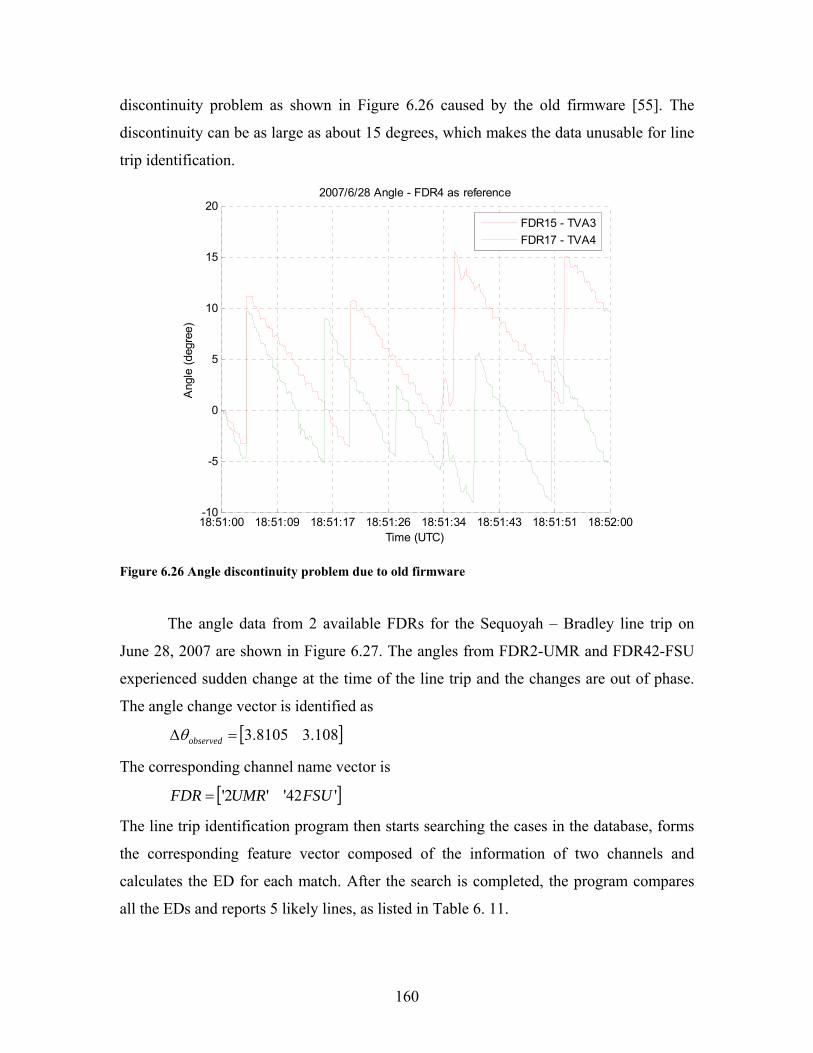
160
discontinuity problem as shown in Figure 6.26 caused by the old firmware [55]. The
discontinuity can be as large as about 15 degrees, which makes the data unusable for line
trip identification.
18:51:00 18:51:09 18:51:17 18:51:26 18:51:34 18:51:43 18:51:51 18:52:00-10
-5
0
5
10
15
20
Time (UTC)
Ang
le (d
egre
e)2007/6/28 Angle - FDR4 as reference
FDR15 - TVA3FDR17 - TVA4
Figure 6.26 Angle discontinuity problem due to old firmware
The angle data from 2 available FDRs for the Sequoyah – Bradley line trip on
June 28, 2007 are shown in Figure 6.27. The angles from FDR2-UMR and FDR42-FSU
experienced sudden change at the time of the line trip and the changes are out of phase.
The angle change vector is identified as
[ ]108.38105.3=∆ observedθ
The corresponding channel name vector is
[ ]'42''2' FSUUMRFDR =
The line trip identification program then starts searching the cases in the database, forms
the corresponding feature vector composed of the information of two channels and
calculates the ED for each match. After the search is completed, the program compares
all the EDs and reports 5 likely lines, as listed in Table 6. 11.
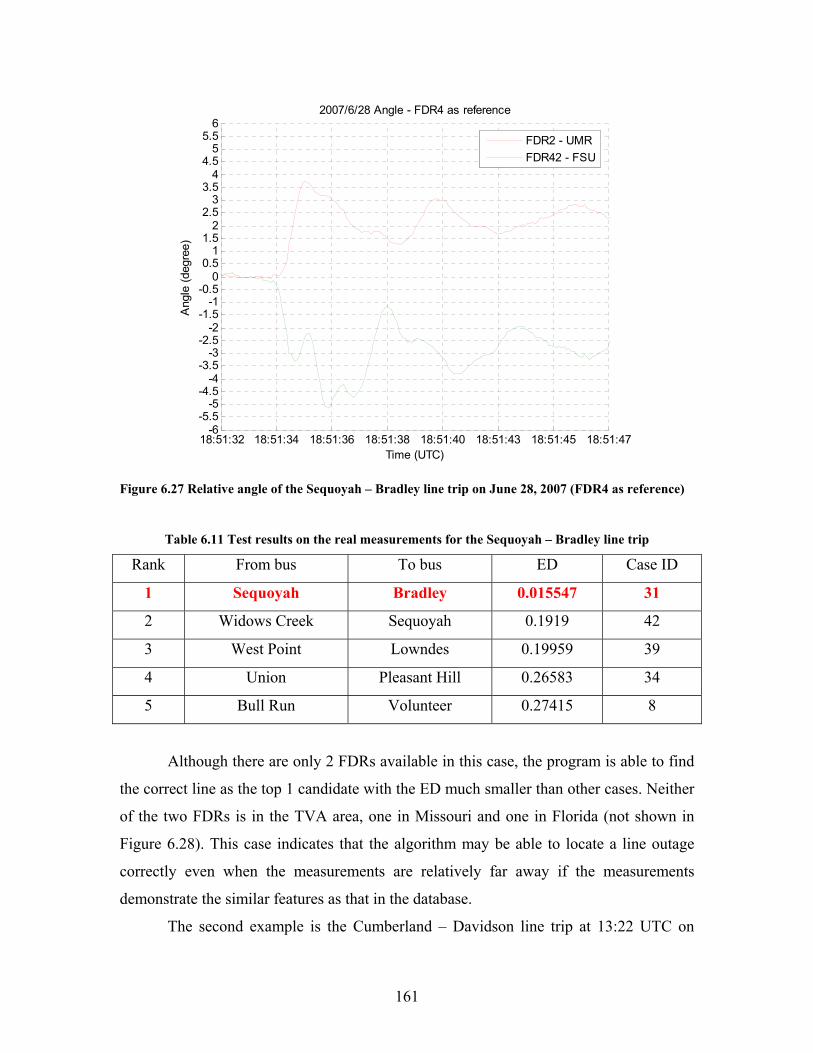
161
18:51:32 18:51:34 18:51:36 18:51:38 18:51:40 18:51:43 18:51:45 18:51:47-6
-5.5-5
-4.5-4
-3.5-3
-2.5-2
-1.5-1
-0.50
0.51
1.52
2.53
3.54
4.55
5.56
Time (UTC)
Ang
le (d
egre
e)
2007/6/28 Angle - FDR4 as reference
FDR2 - UMRFDR42 - FSU
Figure 6.27 Relative angle of the Sequoyah – Bradley line trip on June 28, 2007 (FDR4 as reference)
Table 6.11 Test results on the real measurements for the Sequoyah – Bradley line trip
Rank From bus To bus ED Case ID
1 Sequoyah Bradley 0.015547 31
2 Widows Creek Sequoyah 0.1919 42
3 West Point Lowndes 0.19959 39
4 Union Pleasant Hill 0.26583 34
5 Bull Run Volunteer 0.27415 8
Although there are only 2 FDRs available in this case, the program is able to find
the correct line as the top 1 candidate with the ED much smaller than other cases. Neither
of the two FDRs is in the TVA area, one in Missouri and one in Florida (not shown in
Figure 6.28). This case indicates that the algorithm may be able to locate a line outage
correctly even when the measurements are relatively far away if the measurements
demonstrate the similar features as that in the database.
The second example is the Cumberland – Davidson line trip at 13:22 UTC on
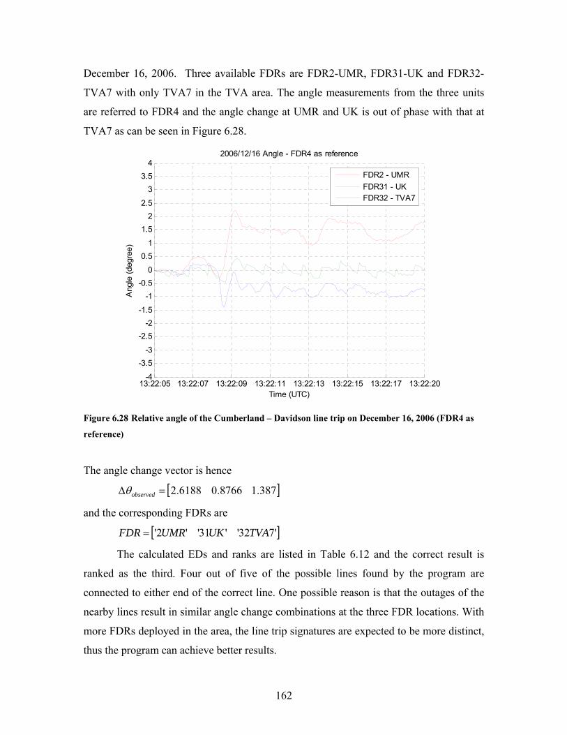
162
December 16, 2006. Three available FDRs are FDR2-UMR, FDR31-UK and FDR32-
TVA7 with only TVA7 in the TVA area. The angle measurements from the three units
are referred to FDR4 and the angle change at UMR and UK is out of phase with that at
TVA7 as can be seen in Figure 6.28.
13:22:05 13:22:07 13:22:09 13:22:11 13:22:13 13:22:15 13:22:17 13:22:20-4
-3.5-3
-2.5-2
-1.5
-1-0.5
0
0.51
1.52
2.5
33.5
4
Time (UTC)
Ang
le (d
egre
e)
2006/12/16 Angle - FDR4 as reference
FDR2 - UMRFDR31 - UKFDR32 - TVA7
Figure 6.28 Relative angle of the Cumberland – Davidson line trip on December 16, 2006 (FDR4 as
reference)
The angle change vector is hence
[ ]1.3870.87662.6188=∆ observedθ
and the corresponding FDRs are
[ ]'732''31''2' TVAUKUMRFDR =
The calculated EDs and ranks are listed in Table 6.12 and the correct result is
ranked as the third. Four out of five of the possible lines found by the program are
connected to either end of the correct line. One possible reason is that the outages of the
nearby lines result in similar angle change combinations at the three FDR locations. With
more FDRs deployed in the area, the line trip signatures are expected to be more distinct,
thus the program can achieve better results.
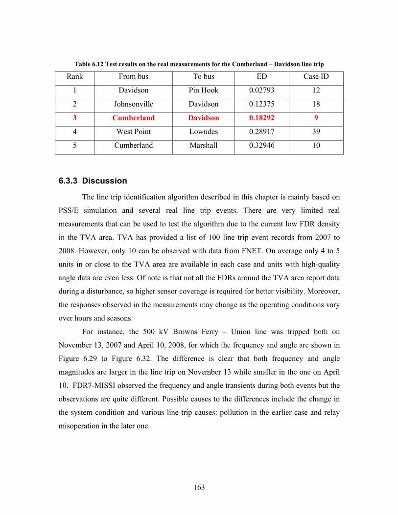
163
Table 6.12 Test results on the real measurements for the Cumberland – Davidson line trip
Rank From bus To bus ED Case ID
1 Davidson Pin Hook 0.02793 12
2 Johnsonville Davidson 0.12375 18
3 Cumberland Davidson 0.18292 9
4 West Point Lowndes 0.28917 39
5 Cumberland Marshall 0.32946 10
6.3.3 Discussion
The line trip identification algorithm described in this chapter is mainly based on
PSS/E simulation and several real line trip events. There are very limited real
measurements that can be used to test the algorithm due to the current low FDR density
in the TVA area. TVA has provided a list of 100 line trip event records from 2007 to
2008. However, only 10 can be observed with data from FNET. On average only 4 to 5
units in or close to the TVA area are available in each case and units with high-quality
angle data are even less. Of note is that not all the FDRs around the TVA area report data
during a disturbance, so higher sensor coverage is required for better visibility. Moreover,
the responses observed in the measurements may change as the operating conditions vary
over hours and seasons.
For instance, the 500 kV Browns Ferry – Union line was tripped both on
November 13, 2007 and April 10, 2008, for which the frequency and angle are shown in
Figure 6.29 to Figure 6.32. The difference is clear that both frequency and angle
magnitudes are larger in the line trip on November 13 while smaller in the one on April
10. FDR7-MISSI observed the frequency and angle transients during both events but the
observations are quite different. Possible causes to the differences include the change in
the system condition and various line trip causes: pollution in the earlier case and relay
misoperation in the later one.
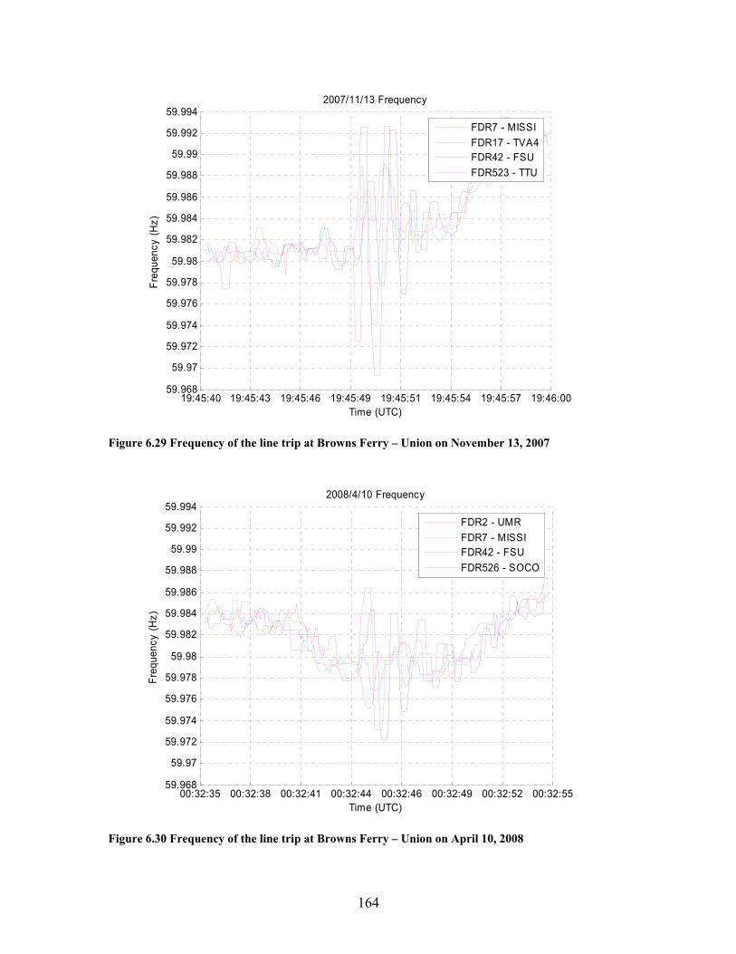
164
19:45:40 19:45:43 19:45:46 19:45:49 19:45:51 19:45:54 19:45:57 19:46:0059.968
59.97
59.972
59.974
59.976
59.978
59.98
59.982
59.984
59.986
59.988
59.99
59.992
59.994
Time (UTC)
Freq
uenc
y (H
z)
2007/11/13 Frequency
FDR7 - MISSIFDR17 - TVA4FDR42 - FSUFDR523 - TTU
Figure 6.29 Frequency of the line trip at Browns Ferry – Union on November 13, 2007
00:32:35 00:32:38 00:32:41 00:32:44 00:32:46 00:32:49 00:32:52 00:32:5559.968
59.97
59.972
59.974
59.976
59.978
59.98
59.982
59.984
59.986
59.988
59.99
59.992
59.994
Time (UTC)
Freq
uenc
y (H
z)
2008/4/10 Frequency
FDR2 - UMRFDR7 - MISSIFDR42 - FSUFDR526 - SOCO
Figure 6.30 Frequency of the line trip at Browns Ferry – Union on April 10, 2008
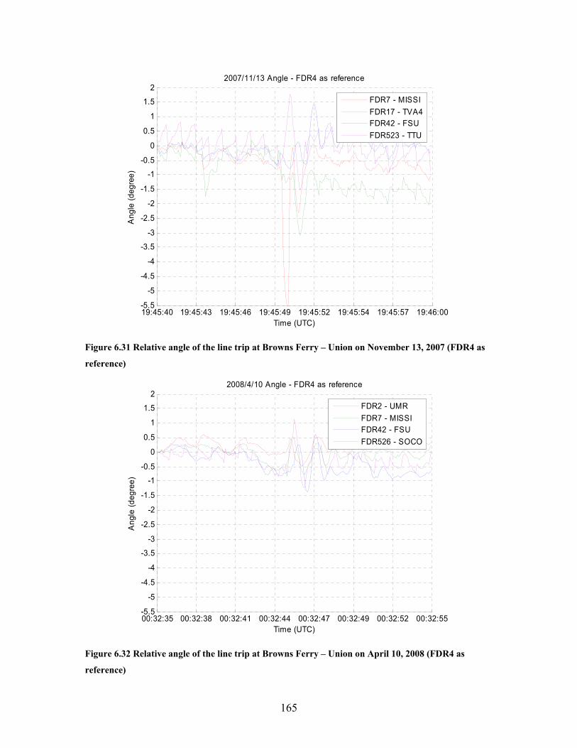
165
19:45:40 19:45:43 19:45:46 19:45:49 19:45:52 19:45:54 19:45:57 19:46:00-5.5
-5
-4.5
-4
-3.5
-3
-2.5
-2
-1.5
-1
-0.5
0
0.5
1
1.5
2
Time (UTC)
Ang
le (d
egre
e)
2007/11/13 Angle - FDR4 as reference
FDR7 - MISSIFDR17 - TVA4FDR42 - FSUFDR523 - TTU
Figure 6.31 Relative angle of the line trip at Browns Ferry – Union on November 13, 2007 (FDR4 as
reference)
00:32:35 00:32:38 00:32:41 00:32:44 00:32:47 00:32:49 00:32:52 00:32:55-5.5
-5
-4.5
-4
-3.5
-3
-2.5
-2
-1.5
-1
-0.5
0
0.5
1
1.5
2
Time (UTC)
Ang
le (d
egre
e)
2008/4/10 Angle - FDR4 as reference
FDR2 - UMRFDR7 - MISSIFDR42 - FSUFDR526 - SOCO
Figure 6.32 Relative angle of the line trip at Browns Ferry – Union on April 10, 2008 (FDR4 as
reference)
166
In future testing and implementation of the identification algorithm, the system
conditions of different seasons should be taken into account. With the growing number of
installed FDRs and confirmed line trip events, it is very possible and practical to improve
the case library with line trips observed in real measurements for different operating
conditions. The correlation between the causes of the line outages and the observed
measurements should be further analyzed in order to improve the case library. An expert
system may be formed for higher accuracy and efficiency.
In addition to the identification algorithm proposed in this chapter, there exist
other methods such as Neural Network for identification of power quality events [67][68]
and pattern recognition for power system security analysis [69][70].
167
Chapter 7 Conclusions and Future Work
7.1 Conclusions
This dissertation has addressed the topic of monitoring the wide-area power
systems at distribution level. Statistical analysis of noticeable disturbances in the three
major North American Interconnections shows that that significant generation-loss like
events are more common than large load-drop like events. Generation-trip like events in
both the EI and the WECC Interconnections are more likely to be encountered in heavy
load season. The event occurrence by hour demonstrates distinct characteristics during
different seasons in the EI and the WECC, which indicates differences in the generation
and load profile and control schemes. On average, the EI experiences a major disturbance
about every 3 days with an estimated generation-load mismatch greater than 500 MW.
The WECC experiences a disturbance almost every 1.5 days with the estimated power
mismatch amount exceeding 200 MW.
Typical frequency disturbance excursions and their possible causes are illustrated.
Loss of generation causes sudden frequency decline. And loss of load induces sharp
frequency rise. Typical frequency excursions differ from each other in the three
Interconnections. Possible reasons include different frequency responses, generation
types, contingency reserve distribution, reserve development, and AGC actions.
A proportional relationship between the largest frequency change rate and total
amount of frequency drop is obtained from theoretical analysis and also verified by the
wide-area measurements. Comparison shows that the ratio by which the two are related is
close in the three major Interconnections: the EI, the WECC and the ERCOT. The linear
relationship between frequency deviation and generation/load mismatch during
disturbances is examined based on exact power mismatch amount in the 129 confirmed
events in the EI, which shows that the frequency response of the system varies in
different seasons as the generation and load profiles change. The inertia and frequency
response characteristics of an Interconnection can be estimated and monitored provided
the information of the actual generation/load mismatch and accurate frequency
measurements. As an application, the estimated frequency response and inertia can be
168
employed to improve the generation/load mismatch calculation in the event detection
program.
Several major disturbances in the EI system are examined including a three-phase
fault in the transmission network, an event involving line events and generator trips, an
islanding incident, the Florida outage, and faults in HVDC systems. Plenty of information
about systems’ response to disturbances, as well as to control actions and protection
schemes is reflected in measurements from distribution networks. The comparison
between measurements from FDR and PMU shows that measurements taken from the
low voltage level demonstrate high quality for monitoring disturbances in the
transmission networks.
The dynamic performances of AC/DC systems are examined. By monitoring the
two ends of the HVDC links, the effects of frequency sensitive damping controls are
observed as the frequency transients at one side are reflected at the other. On the other
hand, it is confirmed in the wide-area measurements that the HVDC links between
asynchronous Interconnections prevents the disturbances in on system form propagating
to another.
With the assist of the visualization techniques, the propagation of disturbances as
electromechanical waves can be better understood. An automated visualization tool has
been developed that can generate frequency and angle replay for disturbances in the EI
system. An attempt has been made to display the steady-state angle distribution in the EI.
Simulation results show that the angle distribution does not follow any obvious
geographically related trend.
Unlike generation or load loss events, line outages generally cause well-damped
oscillations in local frequency and rapid changes in angle. Due to the fact that a single
line trip generally has limited impact on the entire interconnected system, higher sensor
density is required for detecting such disturbances. For the instance of monitoring the
TVA system, 52 sensors (including current and future deployment) are sufficient for
monitoring the major 500 kV transmission lines and part of the 161 kV networks if they
are placed at the proposed locations. Both frequency and angle can be employed as the
line trip detection signals. The detection algorithms developed in the work can be easily
implemented for real-time line trip detection.
169
A signature library for all the single line trip cases at 500 kV in the TVA system
is established with PSS/E simulations. The feature vector for each line trip case is formed
as the angle magnitudes during the first swing at all the observing points. In spite of the
limited sensor coverage and lack of confirmed cases for training the algorithm, the
identification program is tested with simulation and real measurements with reasonable
accuracy. We are aware that the EI model used for simulations is not sufficient to
represent all the operating conditions therefore may be not comprehensive to include all
the possible characteristics of a line outage. However, with the deployment of more
sensors, the signature library can be expanded to represent the line trip disturbances
during different seasons and operating conditions.
7.2 Contributions
This work has made unique contributions in the areas of the wide-area monitoring
of power systems at distribution level and disturbances detection. First, this work
examines the disturbances in the bulk transmission power systems from a wide-area point
of view by providing comparisons of the characteristics of noticeable generation/load loss
events in the three major North American Interconnections both from statistical
perspective and dynamic response perspective. No analysis of this nature has been
presented due to limited access to such wide-area measurements across North America
and data sharing among utilities. The frequency response estimation presented in chapter
2 will help to calibrate the values used in current FNET event detection algorithm thus
improving the power mismatch estimation. The analysis of the various major
disturbances offers valuable insights to the system dynamic responses. A database of the
event signatures shall greatly assist the study of event detection and location estimation,
and further, the design of wide-area controls to prevent severe system failures.
Second, the automated visualization tool using computer graphics designed in this
work improves the power system visualization capabilities by correlates the
measurements with their geographic locations. This dissertation makes the first attempt to
view the phase angle over the Eastern Interconnection both in simulation and
measurements obtained at distribution level. The work in chapter 4 extends the potential
170
applications of angle measurements at lower voltage level, which has been confined
mainly by the uncertainty of the phase shift at each sensor location.
Another major contribution of this work is approaching the line trip detection and
identification based extensively on distribution-level wide-area measurements, which has
not been addressed in previous works. Being aware of the system topology change is
critical because inadvertent line outages can be very dangerous. This work proposes a
methodology with which the topology change in the transmission networks can be
detected and identified based on frequency and angle measurements and simulation
results. The measurement-based algorithms do not require detailed system topology
information which is not readily available in most of the cases. The uniqueness of the
algorithms also lies in the inclusion of the information from both frequency and angle.
Previously, frequency has been examined extensively in various FNET related
applications such as detection of generation/load mismatch disturbances. However, the
detection of line trips can be very difficult if it relies solely on frequency because no
direct relationship is observed between the frequency transients and the closeness of the
monitoring point to the tripped line at least from simulation results. Moreover, the line
loading characteristics may complicate the line outage frequency signature such that
tripping a line connecting to a generator is similar to a generation loss event in frequency.
Phase angles, however, reflect the loading information of transmission lines therefore can
serve as a good detection parameter.
7.3 Potential Future Work
More applications of the wide-area measurements are worth of further
investigation as future research in the areas addressed by this dissertation. The statistical
analysis of the generation/load mismatch events in the North American Interconnections
can be continued to include the ERCOT and the Quebec systems as more FDRs are being
employed in these Interconnections and the number of detected events grows. At the
same time, the frequency response characteristics in the Interconnections should be
continuously monitored which assists not only the improvement of the event detection
program but also the study of system inertia and the electromechanical wave propagation
171
speeds in different Interconnections, which may help to improve the accuracy of event
location estimation.
This work has described the observations in the low-voltage measurements for
several types of major disturbances. This signature library can be expanded by including
more typical disturbances, which can be utilized as a knowledge database for event
classification. The valuable knowledge of the power system dynamics during
disturbances invites future research into areas like mode shapes and controllability.
Moreover, with several HVDC systems in North America being monitored by FNET, the
effects of the HVDC systems on the overall AC/DC system dynamic performance can be
further examined with first-hand measurements to study the controllability of HVDC
system in damping dangerous inter-area oscillations.
In order to better utilize the distribution-level measurements from FNET, more
attention should be paid to calibration of the angle measurements. This work has made
the first attempt to observe directly the angles but more important work is ahead to figure
out the angle shift at each FDR location and adjust it accordingly to make the angle more
meaningful. Thus the advantage of wide sensor coverage of FNET can be fully taken to
observe the hourly or seasonal change in the voltage profile of the large Interconnections.
Besides the phase shifts, there exist discontinuities in angle as shown in chapter 6 which
may be corrected by hardware improvement. Although out of the scope of this
dissertation, the improvement of the angle data quality shall greatly help the disturbance
detection and identification study including the line outage detection. Another
continuation of the topic of angle visualization is to display the angles from the wide-area
view point and provide early warning of stability problems.
This work has developed the algorithms for line trip detection and identification
based on simulation results and real measurements. More training cases are required to
tune the algorithms, which is presently limited by the current sensor coverage in the
target system. The significance of the work in this report is that it has explored and
confirmed the viability of relying on wide-area measurements at distribution level for line
outage detection and identification. Algorithms other than what have been can also be
investigated such as expert system and pattern recognition, etc.

172
Further future research in the area of disturbance detection may include
oscillation detection and mitigation. With the low-cost and easily-deployable power
system monitoring made available by FNET, high sensor density in a regional power
network is within reach. With such wealth of information, it is very realistic to say that
the oscillation patterns or modes are fully exposed and can be exploited for the design of
control and damping systems. As one example, with sufficient number of power system
stabilizers (PSS) in any of the three major Interconnections, wide-area control should
already be close to reality. That is, the coordination of a group of wide spread power
system stabilizer using wide area measurement information is well within our reach and
could be one very attractive study.
173
References [1] J. F. Hauer, N. B. Bhatt, K. Shah, and S. Kolluri, “Performance of “WAMS East” in
providing dynamic information for the North East Blackout of August 14, 2003,”
IEEE Power Engineering Society General Meeting, vol. 2, pp. 1685-1690, 2004.
[2] D. Divan, G. A. Luckjiff, W. E. Brumsickle, J. Freeborg, and A. Bhadkamkar, “A
grid information resource for nationwide real-time power monitoring,” IEEE Trans.
Industry Applications, vol. 40, pp. 699-705, 2004.
[3] A. G. Phadke, “Synchronized phasor measurements in power systems,” IEEE
Computer Applications in Power, vol. 6, pp. 10-15, 1993.
[4] M. Zhou, V. A. Centeno, J. S. Thorp, and A. G. Phadke, “An alternative for including
phasor measurements in state estimators,” IEEE Trans. Power Systems, vol. 21, no. 4,
pp. 1930-1937, Nov. 2006.
[5] W. Jiang, V. Vittal, and G. T. Heydt, “A distributed state estimator utilizing
synchronized phasor measurements,” IEEE Trans. Power Systems., vol. 22, no. 2,
pp.563-571, May 2007.
[6] J. S. Thorp, A. G. Phadke, and K. J. Karimi, “Real time voltage-phasor measurements
for static state estimation,” IEEE Trans. Power App. Syst., vol. PAS-104, no. 11, pp.
3098-3106, Nov. 1985.
[7] G. Zhang, P. Hirsch, and S. Lee, Wide area frequency visualization using smart client
technology,” Proc. IEEE Power Eng. Soc. General Meeting, 2007, pp. 1-8, Jun. 2007.
[8] Z. Zhong, C. Xu, B. J. Billian, L. Zhang, S.-J. S. Tsai, R. W. Conners, V. A. Centeno,
A. G. Phadke, and Y. Liu, “Power System Frequency Monitoring Network (FNET)
implementation,” IEEE Trans. Power Systems, vol. 20, pp. 1914-1921, 2005.
[9] Xia, Tao, Zhang, Hengxu, Gardner, Robert, Bank, Jason, Dong, Jingyuan, Zuo, Jian,
Liu, Yilu, Beard, Lisa, Hirsch, Peter, Zhang, Guorui, and Dong, Rick, “Wide-area
Frequency Based Event Location Estimation,” IEEE Power Engineering Society
General Meeting, pp. 1-7, 2007.
[10] Benmouyal, G., Schweitzer, E.O., and Guzman, A., “Synchronized phasor
measurement in protective relays for protection, control, and analysis of electric
174
power systems,” 2004 57th Annual Conference for Protective Relay Engineers, pp.
419-450.
[11] S. S. Tsai, L. Zhang, A. G. Phadke, Y. Liu, M. R. Ingram, S, C, Bell, I. S. Grant,
D. T. Bradshaw, D. Lubkeman, and L. Tang, “Study of global frequency dynamic
behavior of large power systems,” IEEE PES Power System Conference and
Exposition, New York, pp. 328-335, Oct. 2004.
[12] North America Electric Reliability Council, “Understand and calculate frequency
response,” 2003, NERC Training Resources Working Group.
[13] A. Bykhovsky and J. H. Chow, “Power system disturbance identification from
recorded dynamic data at the Northfield substation,” International Journal Electrical
Power & Energy Systems, vol. 25, pp. 787-795, 2003.
[14] N. Jaleeli, L. S. VanSlysk, “NERC’s new control performance standards,” IEEE
Trans. Power Systems, vol. 14, pp. 1092-1099, 1999.
[15] L.-R. Chang-Chien, Y.-J. Lin, and C.-C Wu, “A real-time contingency reserve
scheduling for an isolated power system,” IEEE Trans. Reliability, to be published.
[16] North America Electric Reliability Council, “2006 Summer assessment reliability
of bulk power systems in North America”. Available at:
http://www.nerc.com/files/summer2006.pdf.
[17] North America Electric Reliability Council, “2006/2007 Winter assessment
reliability of bulk power systems in North America”. Available at:
http://www.nerc.com/files/winter2006-07.pdf.
[18] P. Kundur, Power System Stability and Control, New York: McGraw-Hill, 1994.
[19] T. Inoue, H. Taniguchi, Y. Ikeguchi, and K. Yoshida, “Estimation of power
system inertia constant and capacity of spinning-reserve support generators using
measured frequency transients,” IEEE Trans. Power Systems, vol. 12, pp. 136-143,
1997.
[20] D. P. Chassin, Z. Huang, M. K. Donnelly, C. Hassler, E. Ramirez, and C. Ray,
“Estimation of WECC system inertia using observed frequency transients,” IEEE
Trans. Power Systems, vol. 20, pp. 1190-1192, 2005.
[21] North America Electric Reliability Council, “Disturbance control performance”.
Available at: http://www.nerc.com/files/BAL-002-0.pdf.
175
[22] B.M. Pasternack, and N.B. Bhatt, “The Rockport plant – analysis of temporary
fast turbine valving tests,” IEEE Trans. Power Systems, vol. 3, pp. 529-540, 1988.
[23] Bhatt, N.B., “Field experience with momentary fast turbine valving and other
special stability controls employed at AEP's Rockport plant,” IEEE Trans. Power
Systems, vol. 11, pp. 155-161, 1996
[24] Dalke, G., Baum, A., Bailey, B., Daley, J.M., Duncan, B., Fischer, J., Hesla, E.,
Hoerauf, R., Hornbarger, B., Lee, W.-J.; Love, D.J., McCullough, D., Mozina, C.,
Nichols, N., Padden, L., Patel, S., Al Pierce, Pillai, P., Poletto, G., Rifaat, R., Sanders,
M.K., Shelton, J.M., Stringer, T.N., Weber, J., Wu, A., and Young, R., “Application
of islanding protection for industrial and commercial generators-an IEEE industrial
application society working group report,” 2006 59th Annual Conference for
Protective Relay Engineers, pp. 12.
[25] Hou, D. and Tziouvaras, D.A, “Out-of-step protection enhancements,” 2004
Eighth IEE International Conference on Developments in Power System Protection,
pp. 5-10.
[26] Taylor, C.W., and Lefebvre, S., “HVDC controls for system dynamic
performance,” IEEE Trans. Power Systems, vol. 6, pp. 743-752, 1991.
[27] Report, IC, “Dynamic Performance Characteristics of North American HVDC
Systems for Transient and Dynamic Stability Evaluations,” IEEE Trans. Power
Systems, vol. PAS-100, pp. 3356-3364, 1981.
[28] Samuelsson, O., Hemmingsson, M., Nielsen, A.H., Pedersen, K.O.H., and
Rasmussen, J., "Monitoring of power system events at transmission and distribution
level," IEEE Trans. Power Systems, vol. 21, pp. 1007-1008, 2006.
[29] FRCC, “FRCC Event Analysis Team Interim Recommendations Report”.
Available at
https://www.frcc.com/Reliability/Shared%20Documents/FEAT%20Interim%20Repor
t.pdf.
[30] NERC news release, “NERC Issues Reliability Advisories on February Florida
Outage”. Available at http://www.nerc.com/news_pr.php?npr=102.
[31] NERC, “NERC’s Bulk Power System Event Classification Scale”. Available at
http://www.nerc.com/page.php?cid=5|63|252.
176
[32] The ABB group, “The HVDC Transmission Québec - New England”. Available
at http://www.abb.com/.
[33] Donahue, J.A., Fisher, D.A., Raling, B.D., and Tatro, P.J., “Performance testing
of the Sandy Pond HVDC converter,” IEEE Trans. Power Delivery, vol. 8, pp. 422-
428, 1993.
[34] Manitoba Hydro, “Nelson River DC Transmission System”. Available at
http://www.hydro.mb.ca/corporate/facilities/ts_nelson.shtml.
[35] Dhaliwal, N.S., Recksiedler, L.D., and Tang, D.T.Y., “Operating experiences of
the Nelson River HVDC system,” IEEE Transmission and Distribution Conference,
pp. 174-180, 1996.
[36] Hou, D., and Fischer, N., “Deterministic High-Impedance Fault Detection and
Phase Selection on Ungrounded Distribution Systems,” Power Systems Conference:
Advanced Metering, Protection, Control, Communication, and Distributed Resources,
pp. 112-122, 2006.
[37] Chapman, D.G., and Jost, F.A., “Operation of an isolated hydro plant supplying
an hvdc transmission load,” IEEE Trans. Power Apparatus and Systems, vol. 95, pp.
1099-1104, 1976.
[38] Chand, J., “Auxiliary Power Controls on the Nelson River HVDC scheme,” IEEE
Trans. Power Systems, vol. 7, pp. 398-402, 1992.
[39] Mao, X.M., Zhang, Y., Guan, L., Wu, X.C., and Zhang, N., “Improving power
system dynamic performance using wide-area high-voltage direct current damping
control,” Generation, Transmission & Distribution, IET, vol. 2, pp. 245-251, 1992.
[40] J.S. Thorp, C.E. Seyler, and A.G. Phadke, “Electromechanical wave propagation
in large electric power system”, IEEE Tran. Circuits and Systems I: Fundamental
Theory and Applications, vol. 45, pp. 614-622, 1998.
[41] Overbye, T.J. and Weber, J.D., “Visualizing the electric grid,” IEEE Spectrum,
vol. 38, pp. 52-58, 2001.
[42] Pires de Azevedo, G., Sieckenius de Souza, C. and Feijo, B.; “Enhancing the
human-computer interface of power system applications,” IEEE Trans. Power
Systems, vol. 11, pp. 646-653, 1996.
177
[43] Weber, J.D. and Overbye, T.J., “Voltage contours for power system
visualization,” IEEE Trans. Power Systems, vol. 15, pp. 404-409, 2000.
[44] Naoki Kobayashi, Takeshi Yamada, Hiroshi Okamoto, Yasuyuki Tada, Atsushi
Kurita and Yasuji Sekine, “Visualization of results of load flow calculation and
dynamic simulation,” Electrical Engineering in Japan, vol. 116, pp. 35-48, 1996.
[45] Mota, Ad.A., Mota, L.T.M. and Morelato, A., “Teaching power engineering
basics using advanced web technologies and problem-based learning environment,”
IEEE Trans. Power Systems, vol. 19, pp. 96-103, 2003.
[46] Ohashi, T. and Ono, T., “Visualization and interactive simulation for power
system operation and education,” Fourth International Conference on Advances in
Power System Control, Operation and Management, vol. 2, pp. 802-807, 1997.
[47] Overbye, T.J., “Visualizing the interaction between the transmission system and
power markets,” IEEE Power Engineering Society Summer Meeting, vol. 2, pp. 1019-
1024, 2001.
[48] Lisa S. Avila, Sebastien Barre, Rusty Blue, Berk Geveci, Amy Henderson,
William A. Hoffman, Brad King, C. Charles Law, Kenneth M. Martin, and William J.
Schroeder, The VTK user's guide: updated for VTK version 4.4, Clifton Park, NY:
Kitware Inc., 2004.
[49] Will Schroeder, William Schroeder, Ken Martin, Kenneth William Martin, and
Bill Lorensen, The Visualization Toolkit: An Object-oriented Approach to 3D
Graphics, Clifton Park, NY: Kitware Inc., 2004.
[50] MathTools Ltd. “MIDEVA, MATCOM & Visual MATCOM user’s guide,” 1999.
[51] William Ford and William Topp, Data Structures with C++ and STL, Second
Edition, Prentice Hall, 2001.
[52] J. Zuo, "The Frequency Monitor Network (FNET) Design and Situation
Awareness Algorithm Develop," Ph.D. dissertation, Department of Electrical and
Computer Engineering, Virginia Tech, Blacksburg, 2008.
[53] “Map Projection”. Available at http://en.wikipedia.org/wiki/Map_projection.
[54] S.J.S Tsai, "Study of Global Power System Frequency Behavior Based on
Simulations and FNET Measurements," Ph.D. dissertation, Department of Electrical
and Computer Engineering, Virginia Tech, Blacksburg, 2005.
178
[55] K.J.H. Khan, "Wide Area Power System Monitoring Device Design and Data
Analysis," Master thesis, Department of Electrical and Computer Engineering,
Virginia Tech, Blacksburg, 2006.
[56] http://earth.google.com/.
[57] “KML documentation introduction”. Available at
http://code.google.com/apis/kml/documentation/.
[58] Shankar, M., Stovall, J., Sorokine, A., Bhaduri, B. and King, T., “Visualizing
energy resources dynamically on earth,” IEEE Power Engineering Society General
Meeting, pp. 1-4, 2008.
[59] Wolk, R.M., “Utilizing Google Earth and Google Sketchup to visualize wind
farms,” IEEE International Symposium on Technology and Society, pp. 1-8, 2008.
[60] Weili Ding, Feng Zhu and Yingming Hao, “Interactive 3D City Modeling using
Google Earth and Ground Images,” Fourth International Conference on Image and
Graphics, pp. 849-854, 2007.
[61] Chadil, N., Russameesawang, A. and Keeratiwintakorn, P., “Real-time tracking
management system using GPS GPRS and Google earth,” 5th International
Conference on Electrical Engineering/Electronics, Computer, Telecommunications
and Information Technology, vol. 1, pp. 393-396, 2008.
[62] Bi, T.S., Song, X.N., Wu, J.T. and Yang, Q.X., “Novel method for disturbance
identification in power systems,” IEEE Power Engineering Society General Meeting,
pp. 1-5, 2006.
[63] Power Technologies, INC, PSS/E-29 Program Operation Manual: Volume I,
Schenectady, NY, 2002, pp. 7-27.
[64] Power Technologies, INC, PSS/E-29 Application Guide: Volume I, Schenectady,
NY, 2002, pp. 1-2.
[65] Wood, A.J. and Wollenberg, B.F., Power Generation, Operation and Control:
Second Edition, New York, NY: John Wiley & Sons, Inc, 1996, pp. 107.
[66] Hazra, J. and Sinha, A.K., “Identification of catastrophic failure in power systems
using pattern recognition,” IEEE Power India Conference, pp. 1-7, 2006.

179
[67] Santoso, S., Powers, E.J., Grady, W.M. and Parsons, A.C., “Power quality
disturbance waveform recognition using wavelet-based neural classifier. I.
Theoretical foundation,” IEEE Trans. Power Delivery, vol. 15, pp. 222-228, 2000.
[68] Santoso, S., Powers, E.J., Grady, W.M. and Parsons, A.C., “Power quality
disturbance waveform recognition using wavelet-based neural classifier. II.
Application,” IEEE Trans. Power Delivery, vol. 15, pp. 229-235, 2000.
[69] Pang, Chok K., Koivo, Antti J. and El-Abiad, Ahmed H.; “Application of Pattern
Recognition to Steady-State Security Evaluation in a Power System,” IEEE Trans.
Systems, Man and Cybernetics, vol. 3, pp. 622-631, 1973.
[70] Chang, C.S., Chung, T.S. and Lo, K.L., “Application of pattern recognition
technique to power system security analysis and optimization,” IEEE Trans. Power
Systems, vol. 5, pp. 835-841, 1990.
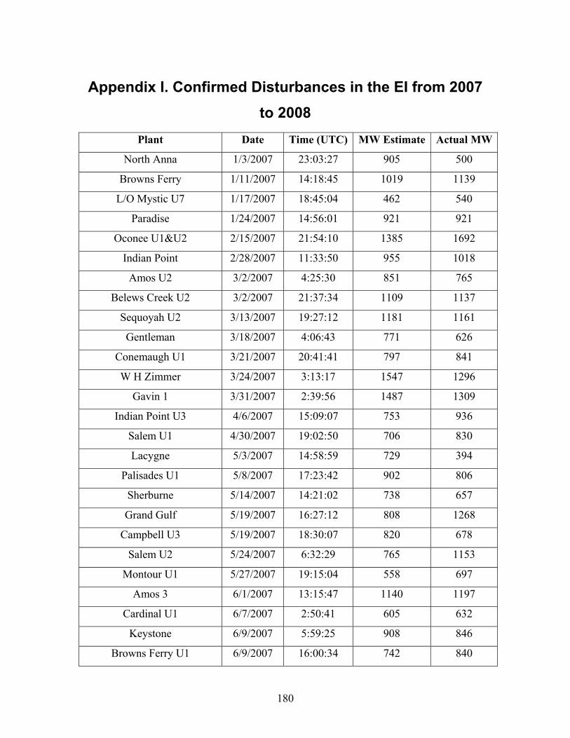
180
Appendix I. Confirmed Disturbances in the EI from 2007 to 2008
Plant Date Time (UTC) MW Estimate Actual MW
North Anna 1/3/2007 23:03:27 905 500
Browns Ferry 1/11/2007 14:18:45 1019 1139
L/O Mystic U7 1/17/2007 18:45:04 462 540
Paradise 1/24/2007 14:56:01 921 921
Oconee U1&U2 2/15/2007 21:54:10 1385 1692
Indian Point 2/28/2007 11:33:50 955 1018
Amos U2 3/2/2007 4:25:30 851 765
Belews Creek U2 3/2/2007 21:37:34 1109 1137
Sequoyah U2 3/13/2007 19:27:12 1181 1161
Gentleman 3/18/2007 4:06:43 771 626
Conemaugh U1 3/21/2007 20:41:41 797 841
W H Zimmer 3/24/2007 3:13:17 1547 1296
Gavin 1 3/31/2007 2:39:56 1487 1309
Indian Point U3 4/6/2007 15:09:07 753 936
Salem U1 4/30/2007 19:02:50 706 830
Lacygne 5/3/2007 14:58:59 729 394
Palisades U1 5/8/2007 17:23:42 902 806
Sherburne 5/14/2007 14:21:02 738 657
Grand Gulf 5/19/2007 16:27:12 808 1268
Campbell U3 5/19/2007 18:30:07 820 678
Salem U2 5/24/2007 6:32:29 765 1153
Montour U1 5/27/2007 19:15:04 558 697
Amos 3 6/1/2007 13:15:47 1140 1197
Cardinal U1 6/7/2007 2:50:41 605 632
Keystone 6/9/2007 5:59:25 908 846
Browns Ferry U1 6/9/2007 16:00:34 742 840

181
Plant Date Time (UTC) MW Estimate Actual MW
Belews Creek U1 6/12/2007 15:40:52 870 1137
Iatan U1 6/16/2007 4:50:52 697 658
Belews Creek U2 6/19/2007 5:09:01 693 1050
Cumberland 6/23/2007 14:23:10 1052 1200
Keystone 6/27/2007 8:50:07 774 807
Braidwood 6/27/2007 14:21:13 875 1236
Darlington U1 6/29/2007 17:35:12 713 1000
North Anna2 6/29/2007 21:53:56 864 954
Conemaugh 7/1/2007 23:34:16 756 849
Amos U3 7/2/2007 16:49:42 1076 1262
Bulls Run U1 7/3/2007 13:55:35 663 900
Gavin U1 7/4/2007 13:27:43 1038 1286
Iatan U1 7/7/2007 20:37:54 570 663
Cumberland U1 7/17/2007 0:40:22 934 1269
Cumberland U1 7/21/2007 2:44:25 686 501
Baldwin U1 7/25/2007 19:01:41 872 587
Rockport,Petersburg,Newton 8/4/2007 21:44:14 2387 4000
Salem U2 8/6/2007 17:11:22 952 1150
Amos U3 8/6/2007 19:39:22 1037 1298
Belews Creek U2 8/10/2007 4:57:41 1003 1135
Seminole U1,2,3(SPP) 8/16/2007 3:26:58 690 1195
Braidwood Nuclear 8/18/2007 19:10:21 685 919
Braidwood U2 8/23/2007 20:30:52 870 1112
Cumberland U2 8/24/2007 7:50:13 691 893
Donald C. Cook U1 8/28/2007 17:53:13 921 1060
Mountaineer U1 9/1/2007 13:48:00 1089 1297
Rockport U2 9/4/2007 16:57:07 745 1331
Jeffrey Energy Center U2 U3 10/3/2007 15:26:37 1112 1376
New Madrid U2 10/20/2007 9:50:29 714 559
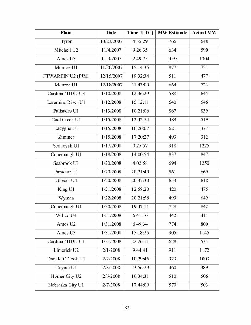
182
Plant Date Time (UTC) MW Estimate Actual MW
Byron 10/23/2007 4:35:29 766 648
Mitchell U2 11/4/2007 9:26:35 634 590
Amos U3 11/9/2007 2:49:25 1095 1304
Monroe U1 11/20/2007 15:14:35 877 754
FTWARTIN U2 (PJM) 12/15/2007 19:32:34 511 477
Monroe U1 12/18/2007 21:43:00 664 723
Cardinal/TIDD U3 1/10/2008 12:36:29 588 645
Laramine River U1 1/12/2008 15:12:11 640 546
Palisades U1 1/13/2008 10:21:06 867 839
Coal Creek U1 1/15/2008 12:42:54 489 519
Lacygne U1 1/15/2008 16:26:07 621 377
Zimmer 1/15/2008 17:20:27 493 312
Sequoyah U1 1/17/2008 0:25:57 918 1225
Conemaugh U1 1/18/2008 14:00:54 837 847
Seabrook U1 1/20/2008 4:02:58 694 1250
Paradise U1 1/20/2008 20:21:40 561 669
Gibson U4 1/20/2008 20:37:30 653 618
King U1 1/21/2008 12:58:20 420 475
Wyman 1/22/2008 20:21:58 499 649
Conemaugh U1 1/30/2008 19:47:11 728 842
Willco U4 1/31/2008 6:41:16 442 411
Amos U2 1/31/2008 6:49:34 774 800
Amos U3 1/31/2008 15:18:25 905 1145
Cardinal/TIDD U1 1/31/2008 22:26:11 628 534
Limerick U2 2/1/2008 9:44:41 911 1172
Donald C Cook U1 2/2/2008 10:29:46 923 1003
Coyote U1 2/3/2008 23:56:29 460 389
Homer City U2 2/6/2008 16:34:31 510 506
Nebraska City U1 2/7/2008 17:44:09 570 503
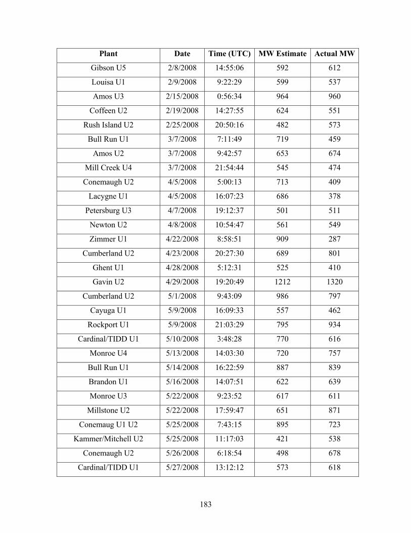
183
Plant Date Time (UTC) MW Estimate Actual MW
Gibson U5 2/8/2008 14:55:06 592 612
Louisa U1 2/9/2008 9:22:29 599 537
Amos U3 2/15/2008 0:56:34 964 960
Coffeen U2 2/19/2008 14:27:55 624 551
Rush Island U2 2/25/2008 20:50:16 482 573
Bull Run U1 3/7/2008 7:11:49 719 459
Amos U2 3/7/2008 9:42:57 653 674
Mill Creek U4 3/7/2008 21:54:44 545 474
Conemaugh U2 4/5/2008 5:00:13 713 409
Lacygne U1 4/5/2008 16:07:23 686 378
Petersburg U3 4/7/2008 19:12:37 501 511
Newton U2 4/8/2008 10:54:47 561 549
Zimmer U1 4/22/2008 8:58:51 909 287
Cumberland U2 4/23/2008 20:27:30 689 801
Ghent U1 4/28/2008 5:12:31 525 410
Gavin U2 4/29/2008 19:20:49 1212 1320
Cumberland U2 5/1/2008 9:43:09 986 797
Cayuga U1 5/9/2008 16:09:33 557 462
Rockport U1 5/9/2008 21:03:29 795 934
Cardinal/TIDD U1 5/10/2008 3:48:28 770 616
Monroe U4 5/13/2008 14:03:30 720 757
Bull Run U1 5/14/2008 16:22:59 887 839
Brandon U1 5/16/2008 14:07:51 622 639
Monroe U3 5/22/2008 9:23:52 617 611
Millstone U2 5/22/2008 17:59:47 651 871
Conemaug U1 U2 5/25/2008 7:43:15 895 723
Kammer/Mitchell U2 5/25/2008 11:17:03 421 538
Conemaugh U2 5/26/2008 6:18:54 498 678
Cardinal/TIDD U1 5/27/2008 13:12:12 573 618
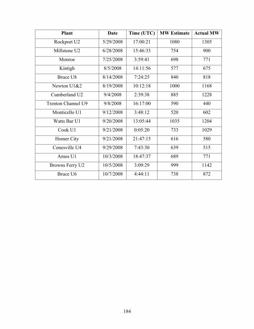
184
Plant Date Time (UTC) MW Estimate Actual MW
Rockport U2 5/29/2008 17:00:21 1080 1305
Millstone U2 6/28/2008 15:46:33 754 900
Monroe 7/25/2008 3:59:41 698 771
Kintigh 8/5/2008 14:11:56 577 675
Bruce U8 8/14/2008 7:24:25 840 818
Newton U1&2 8/19/2008 10:12:18 1000 1168
Cumberland U2 9/4/2008 2:39:38 885 1228
Trenton Channel U9 9/8/2008 16:17:00 590 440
Monticello U1 9/12/2008 3:48:12 520 602
Watts Bar U1 9/20/2008 13:05:44 1035 1204
Cook U1 9/21/2008 0:05:20 733 1029
Homer City 9/21/2008 21:47:15 616 580
Conesville U4 9/29/2008 7:43:30 639 515
Amos U1 10/3/2008 18:47:37 689 771
Browns Ferry U2 10/5/2008 3:09:29 999 1142
Bruce U6 10/7/2008 4:44:11 738 872

185
Appendix II. Development Manual for the Visualization Tool
1. Install the Visualization Toolkit (VTK)
The information for installing the Visualization Toolkit (VTK) can be found in
chapter 1 and chapter 2 of ‘The VTK User’s Guide Updated for Version 5’. VTK
compiles and runs on many different computer platforms. In this program, VTK
applications are developed in Windows platform using Microsoft Visual C ++
(MSVC++). To install VTK, the source code will have to be compiled to produce
libraries and executables. To develop C++ applications and extend VTK, a source code
installation is needed. The machine must be running Windows95, Windows98, Windows
ME, Windows NT 4.0, Windows 2000 or Windows XP. A C++ compiler should be
installed on the computer.
(1) Get the source code
The current program is using VTK 5.0. The latest release of VTK source code can
be downloaded from http://www.vtk.org/get-software.php.
(2) Install CMake
CMake is an open-source, cross-platform Make tool for configuring and
managing the build process. Simple, platform independent files (CMakeLists.txt) are
used to describe the build process and capture dependencies. When CMake is run, it
produces native build files for the particular compiler/operating system. For example, on
Windows MS Visual C ++ workspaces are created.
(Learn more about CMake at http://www.cmake.org; download CMake from
http://www.cmake.org/HTML/Download.html.)
(3) Run CMake
After installation, there should be a CMake entry in the Start menu under
Programs->CMake->CMakeSetup. Running CMake requires three basic pieces of
information: where the source code directory is, which directory to place the binaries
(these are generated as a result of compiling the source code), and which compiler to use.
The CMake interface is shown in Figure II.1. CMake is used to generate projects,
186
makefiles, or workspace. It runs with a GUI that allows users to easily set compile flags.
These flags can be set by left-mouse clicking in the building flag value. The directories
can be specified with the ‘Browse’ button. After that, click once the ‘Configure’ button.
CMake will display a dialog from which you can select the compiler. At this point, one
can customize the variables. After that, click the ‘Configure’ button again, until all the
variables are satisfactory and colored grey. Then click the ‘OK’ button.
Figure II. 1 Run Cmake to build the VTK libraries
(4) Build the library
For Microsoft, a project file will be located in the specified binary path. Simply
load this project file (VTK.sln for .NET), select the ALL_BUILD project, and compile it.
The MSVC++ interface is shown in Figure II.2. (Note: Do not use the MSVC++ ‘Rebuild
All’ menu to rebuild the source code. This deletes all CMakeLists.txt files which are then
automatically regenerated as part of the build progress. MSVC++ will then try reloading
them and an error will result. Instead, to rebuild everything, remove the VTK binary
directory, rerun CMake, and then do a normal build.)

187
Figure II. 2 Build the VTK libraries in MSVC++
2. Install and Configure MATCOM Math Library
(1) Install MATCOM
Run mat4501vc.exe, a widow will appear as shown in Figure II.3. The default
installation directory is C:\matcom45. During installation, the software will ask if Matlab
has been installed on the machine, answer NO to this question. It also requires a file
cl.exe, which can be found at C:\Program Files\Microsoft Visual Studio .NET
2003\Vc7\bin; if Microsoft Visual Studio. NET has been installed with default directory.
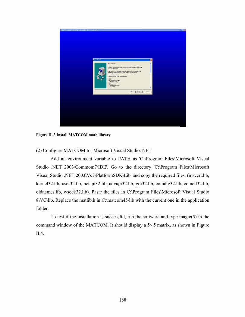
188
Figure II. 3 Install MATCOM math library
(2) Configure MATCOM for Microsoft Visual Studio. NET
Add an environment variable to PATH as 'C:\Program Files\Microsoft Visual
Studio .NET 2003\Commom7\IDE'. Go to the directory 'C:\Program Files\Microsoft
Visual Studio .NET 2003\Vc7\PlatformSDK\Lib' and copy the required files. (msvcrt.lib,
kernel32.lib, user32.lib, netapi32.lib, advapi32.lib, gdi32.lib, comdlg32.lib, comctl32.lib,
oldnames.lib, wsock32.lib). Paste the files in C:\Program Files\Microsoft Visual Studio
8\VC\lib. Replace the matlib.h in C:\matcom45\lib with the current one in the application
folder.
To test if the installation is successful, run the software and type magic(5) in the
command window of the MATCOM. It should display a 5×5 matrix, as shown in Figure
II.4.
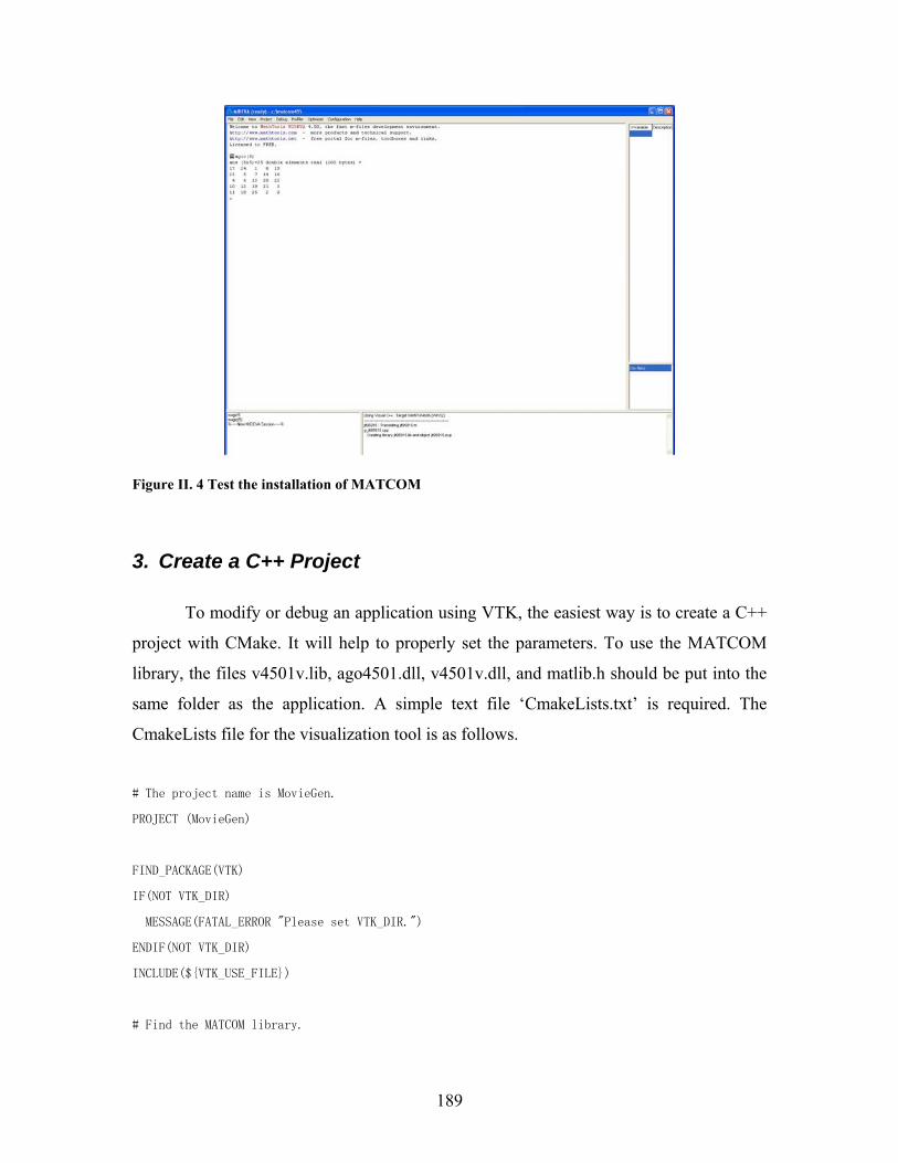
189
Figure II. 4 Test the installation of MATCOM
3. Create a C++ Project
To modify or debug an application using VTK, the easiest way is to create a C++
project with CMake. It will help to properly set the parameters. To use the MATCOM
library, the files v4501v.lib, ago4501.dll, v4501v.dll, and matlib.h should be put into the
same folder as the application. A simple text file ‘CmakeLists.txt’ is required. The
CmakeLists file for the visualization tool is as follows.
# The project name is MovieGen.
PROJECT (MovieGen)
FIND_PACKAGE(VTK)
IF(NOT VTK_DIR)
MESSAGE(FATAL_ERROR "Please set VTK_DIR.")
ENDIF(NOT VTK_DIR)
INCLUDE(${VTK_USE_FILE})
# Find the MATCOM library.

190
FIND_LIBRARY(matcom NAMES v4501v PATHS C:/matcom45/lib)
# Link the libraries
LINK_LIBRARIES(
vtkRendering
vtkGraphics
vtkImaging
vtkIO
vtkFiltering
vtkCommon
v4501v
)
# Include the header and source files
SET(SRCS
movie.h
ReadData.h
Movie.cpp
ReadData.cpp
)
ADD_EXECUTABLE(AutoMovie ${SRCS})
Put the CmakeList.txt file and other header and sources files in a same directory.
In this case, the files are movie.h, ReadData.h, Movie.cpp, and ReadData.cpp. Each file
will be discussed in detail.
Then run CMake. Select the source and binary directories as the same one. A
MSVC++ project will be established in the specified directory. By opening the
MovieGen.sln, one can modify the header and source files, or debug and compile the
project.

191
4. The Structure of the Program
As mentioned in section 3, this program includes two header files and two source
files. Functions to read measurement data and location information are declared in
ReadData.h. The functions are as follows.
void ReadUnitConfig() – read unit information fro UnitConfig.txtp;
void ReadEventLocation() – read event time and location information from EventLocation.txt;
void FormatTime() – format time;
void ReadEventData() - read and treat event data from generated text files;
void ReadOneUnitData() - read data from one file;
void MovingMedian() - moving median process;
void combsort() - sort data (used in moving median);
void DataCondition() - remove noises;
void TreatDelay() - find and treat units with 1-second delay.
The file ReadData.h also declared some structures and vectors to hold and pass
data. The definition of each function is in the file ReadData.cpp. The file movie.h also
declares functions to process frequency data and visualize them. Following are the
functions. The specific definition of the functions can be found in Movie.cpp.
static vtkWindowToImageFilter *ImgRender() – form each movie frame;
Mm GenMesh() – MATCOM function to interpolate frequency data and form measurement matrix.
To use classes and functions in VTK, corresponding header files should be
included in the established C++ project. All required VTK header files are included in
movie.h. They have similar names as ‘vtkClassName.h’.
The file ‘matlib.h’ is included to use the MATCOM library. The Matrix<LIB>
matrix type is called Mm. For example, XI, YI, minFreq and maxFreq are declared as
Mm XI, YI;
Mm minFreq, maxFreq;
192
Besides them, MATCOM has over 300 mathematical functions. Refer to the
MATCOM manual for more information.
Read Data
The procedure of reading data is illustrated in Figure II.5.
Figure II. 5 Procedures to read data
1) ReadUnitConfig( ) - Read Unit Configuration
The FDR information is obtained from the "UnitConfig.txt" file by
ReadUnitConfig( ). Then, the FDR information is stored in the global vectors defined in
ReadData.cpp as below. The format of UnitConfig.txt can be found in Figure II.6. So far
only the Eastern Interconnecton is considered in this visualization program.
vector<FDRInfo> EastFDR; // for East Units
vector<FDRInfo> WeccFDR; // for WECC Units
vector<FDRInfo> TxFDR; // for Texas Units
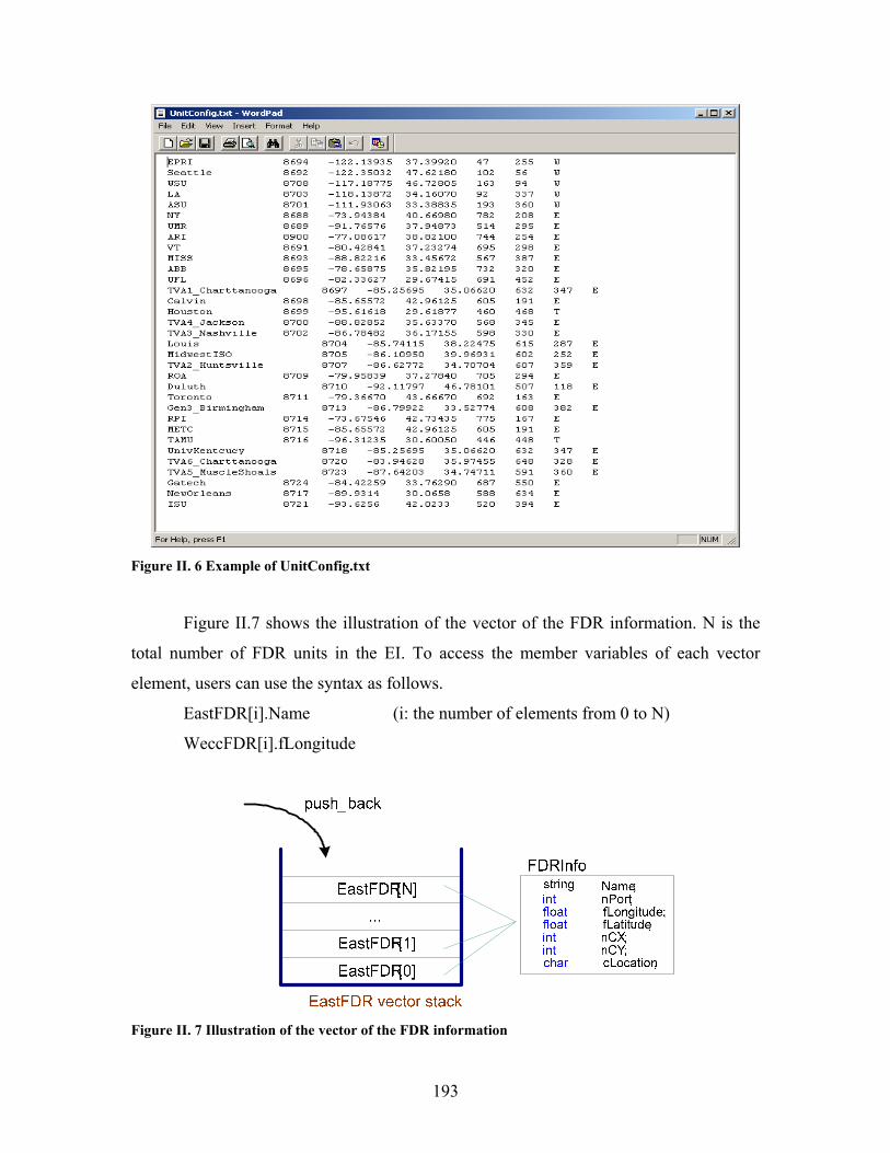
193
Figure II. 6 Example of UnitConfig.txt
Figure II.7 shows the illustration of the vector of the FDR information. N is the
total number of FDR units in the EI. To access the member variables of each vector
element, users can use the syntax as follows.
EastFDR[i].Name (i: the number of elements from 0 to N)
WeccFDR[i].fLongitude
Figure II. 7 Illustration of the vector of the FDR information
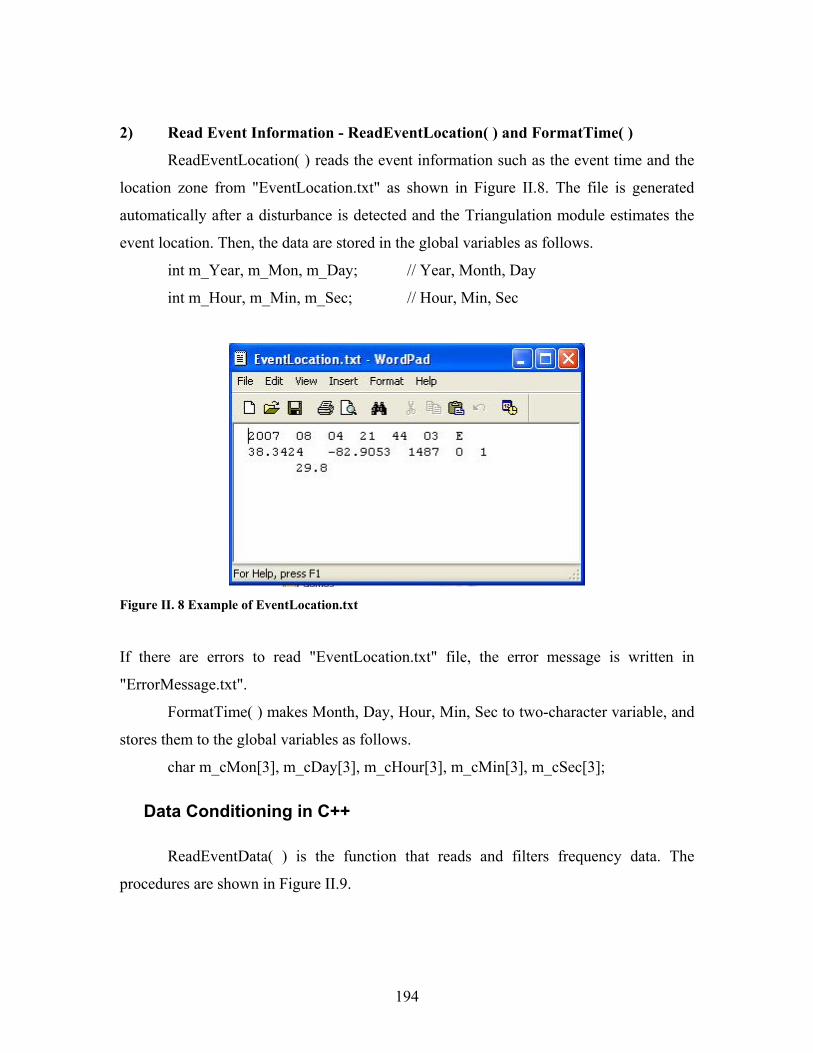
194
2) Read Event Information - ReadEventLocation( ) and FormatTime( )
ReadEventLocation( ) reads the event information such as the event time and the
location zone from "EventLocation.txt" as shown in Figure II.8. The file is generated
automatically after a disturbance is detected and the Triangulation module estimates the
event location. Then, the data are stored in the global variables as follows.
int m_Year, m_Mon, m_Day; // Year, Month, Day
int m_Hour, m_Min, m_Sec; // Hour, Min, Sec
Figure II. 8 Example of EventLocation.txt
If there are errors to read "EventLocation.txt" file, the error message is written in
"ErrorMessage.txt".
FormatTime( ) makes Month, Day, Hour, Min, Sec to two-character variable, and
stores them to the global variables as follows.
char m_cMon[3], m_cDay[3], m_cHour[3], m_cMin[3], m_cSec[3];
Data Conditioning in C++
ReadEventData( ) is the function that reads and filters frequency data. The
procedures are shown in Figure II.9.
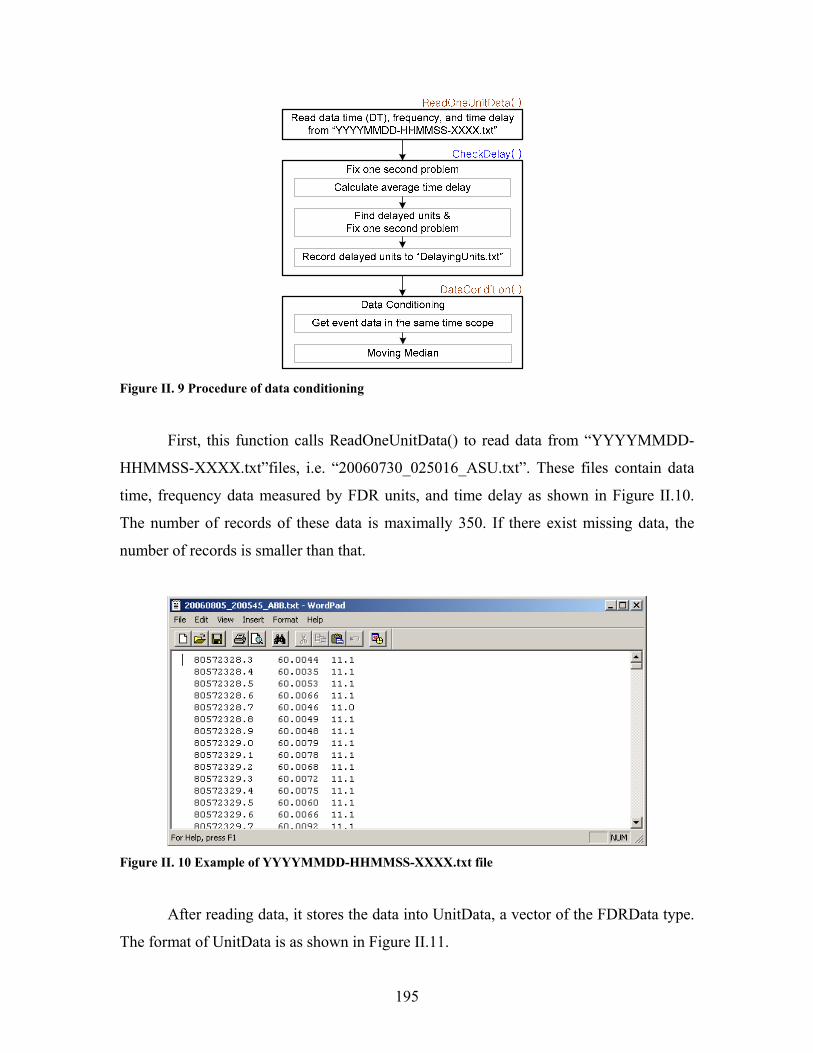
195
Figure II. 9 Procedure of data conditioning
First, this function calls ReadOneUnitData() to read data from “YYYYMMDD-
HHMMSS-XXXX.txt”files, i.e. “20060730_025016_ASU.txt”. These files contain data
time, frequency data measured by FDR units, and time delay as shown in Figure II.10.
The number of records of these data is maximally 350. If there exist missing data, the
number of records is smaller than that.
Figure II. 10 Example of YYYYMMDD-HHMMSS-XXXX.txt file
After reading data, it stores the data into UnitData, a vector of the FDRData type.
The format of UnitData is as shown in Figure II.11.
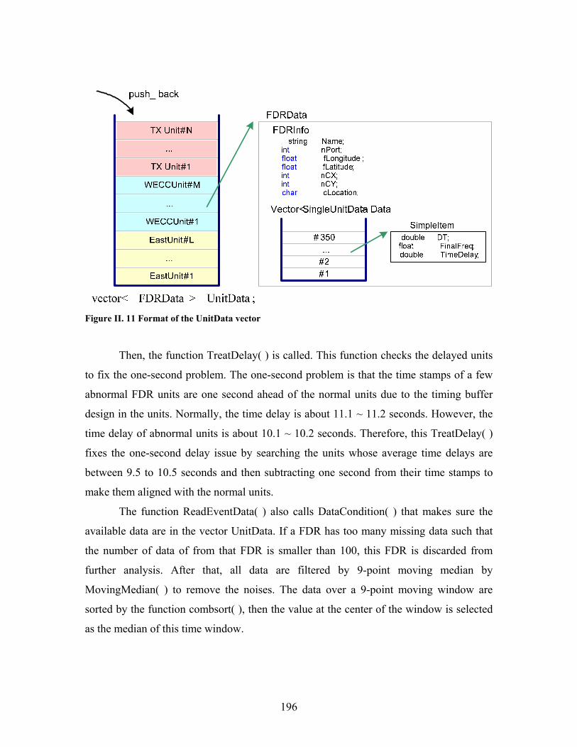
196
Figure II. 11 Format of the UnitData vector
Then, the function TreatDelay( ) is called. This function checks the delayed units
to fix the one-second problem. The one-second problem is that the time stamps of a few
abnormal FDR units are one second ahead of the normal units due to the timing buffer
design in the units. Normally, the time delay is about 11.1 ~ 11.2 seconds. However, the
time delay of abnormal units is about 10.1 ~ 10.2 seconds. Therefore, this TreatDelay( )
fixes the one-second delay issue by searching the units whose average time delays are
between 9.5 to 10.5 seconds and then subtracting one second from their time stamps to
make them aligned with the normal units.
The function ReadEventData( ) also calls DataCondition( ) that makes sure the
available data are in the vector UnitData. If a FDR has too many missing data such that
the number of data of from that FDR is smaller than 100, this FDR is discarded from
further analysis. After that, all data are filtered by 9-point moving median by
MovingMedian( ) to remove the noises. The data over a 9-point moving window are
sorted by the function combsort( ), then the value at the center of the window is selected
as the median of this time window.

197
Generate Measurement Matrix for Display
Frequency measurements from limited number of FDR units are interpolated over
the whole EI area. The area defined by -105 and -66 degrees longitude, and 24 to 52
degrees latitude, is divided into N×M small mesh grids. The longitudes and latitudes are
used directly here because the program assumes Simple Cylindrical projection method to
display FDRs on a map image.
The function Mm GenMesh( ) processes frequency and location data to form a
N×M measurement matrix. This function employs the functions in MATCOM, such as
mean( ), meshgrid( ), and griddata( ). The MATCOM library enables useers to
conveniently use math functions in the similar fashion as in Matlab, which saves coding
time. However, the griddata() function in MATCOM provides only simple interpolation
methods such as nearest neighbor or linear. Before accessing any MATCOM library
functionality, call initM on application initialization. Call exitM before the application
terminates in order to finalize the library. initM may be called multiple times as it is
protected by a static variable. MATCOM_VERSION is a constant defined in matlib.h,
which assures that the versions of the library DLL and matlib.h match. The following is
the initialization of the MATCOM library in the program.
initM(MATCOM_VERSION); //initialize the MATCOM library
……
exitM(); //exit the MATCOM library
The main procedures to generate the measurement matrix are shown in Figure
II.12. And the corresponding codes are as follows.
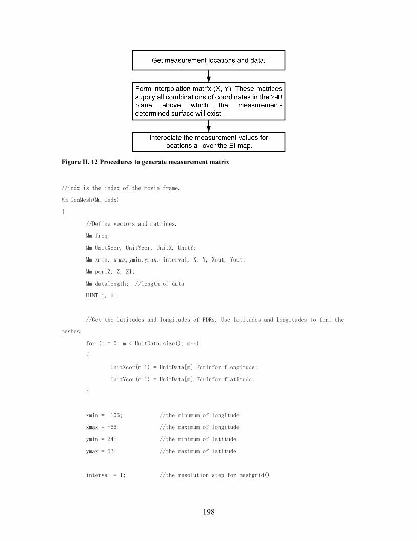
198
Figure II. 12 Procedures to generate measurement matrix
//indx is the index of the movie frame. Mm GenMesh(Mm indx)
{
//Define vectors and matrices.
Mm freq;
Mm UnitXcor, UnitYcor, UnitX, UnitY;
Mm xmin, xmax,ymin,ymax, interval, X, Y, Xout, Yout;
Mm periZ, Z, ZI;
Mm datalength; //length of data
UINT m, n;
//Get the latitudes and longitudes of FDRs. Use latitudes and longitudes to form the
meshes.
for (m = 0; m < UnitData.size(); m++)
{
UnitXcor(m+1) = UnitData[m].FdrInfor.fLongitude;
UnitYcor(m+1) = UnitData[m].FdrInfor.fLatitude;
}
xmin = -105; //the minumum of longitude
xmax = -66; //the maximum of longitude
ymin = 24; //the minimum of latitude
ymax = 52; //the maximum of latitude
interval = 1; //the resolution step for meshgrid()

199
//Prepare the boundary vectors X, Y.
X =
(BR(colon(xmin,interval,xmax)),colon(xmin,interval,xmax),xmin*ones(1.0,length(colon(ymin,interva
l,ymax))),xmax*ones(1.0,length(colon(ymin,interval,ymax))));
Y =
(BR(ymin*ones(1.0,length(colon(xmin,interval,xmax)))),ymax*ones(1.0,length(colon(xmin,interval,x
max))),colon(ymin,interval,ymax),colon(ymin,interval,ymax));
//Prepare the location vectors for meshgrid: Connect X and UnitXcor; Connect Y and
UnitYcor.
Xout = (BR(X),UnitXcor);
Yout = (BR(Y),UnitYcor);
//Form matrices (X,Y) for interpolation
meshgrid(colon(xmin,interval,xmax),colon(ymin,interval,ymax),i_o,XI,YI);
//Form frequency matrix for visualization
datalength = 1200; //number of data points
for (m = 0; m < UnitData.size(); m++)
{
for (n=0; n < datalength.r(); n++)
{
freq(n+1,m+1) = UnitData[m].Data[n].FinalFreq;
}
}
//Find minimum and maxmum frequency values for color mapping
minFreq = mmin(mmin(freq));
maxFreq = mmax(mmax(freq));
//Form frequency vector for boundary:average frequency of FDR measurements
periZ = mean(freq(indx,c_p))*ones(1.0,length(Y));
//Form frequency vector for griddata: connect boundary frequency and frequency
measurements
Z = (BR(periZ),freq(indx,c_p));

200
//Form interpolation matrix with griddata(), interpolation method: linear
ZI = griddata(Xout,Yout,Z,XI,YI,TM("linear"));
//Return the interpolated matrix
return ZI;
}
Form Movie Frames
The function GenMesh( ) prepares the interpolated measurement matrix that can
be used by the function vtkWindowToImageFilter *ImgRender( ). This function utilizes
the classes in the VTK library to generate movie frames and save them to an AVI file.
The visualization tool uses an instance of vtkPolyData to represent measurements.
The coordinates of each measurement are represented by points, and the corresponding
frequency values are represented by the scalars. Then vtkLookupTable maps the
frequency scalars to colors. Finally vtkActor represents all the geometries (lines, points,
etc.) in a render window.
Some graphic models and their functionalities are
• RenderWindow - contains final image
• Renderer - draws into render window
• Actor - combines properties / geometry
• Mappers - represent geometry
• Transformations - position actors
It is simple to use the pre-defined classes in VTK, which involves creating an
instance of a certain class, calling the member functions by defined pointers, and deleting
the pointer to release memory. Following is an example.
vtkPolyData *Surf = vtkPolyData::New(); //Create an instance of vtkPolyData
Surf->SetPoints(points); //Set points to the polydata.
Surf->Delete(); //Delete the pointer after using it.

201
The procedures to generate one movie frame are shown in Figure II.13. The
function vtkWindowToImageFilter *ImgRender( ) obtains data and time stamps for each
frame from the main function, and returns each generated image to the main function.
The frames are then written into an AVI file with vtkAVIWriter. Some vtk-format files
are read by the function to mask out irrelevant areas and display the state borders and
coast lines. They are
EI-border.vtk – defines the borders of states in EI, to be displayed in black.
EI-landmask.vtk – defines the land area outside EI, to be masked in dark grey.
EI-ocean-lake-new.vtk – defines the ocean and lake areas, to be masked in blue.
Represent measurements with vtkPolyData (location coordinates as points, frequency as scalars)
Triangulate the points with vtkDelaunay2D
Map frequency scalars to colors with vtkLookupTable
Map the output polydata to vtkPolyDataMapper
Add a color bar to the rendering widow with vtkScalarBarActor
Add text of event information with vtkTextProperty
Display active FDR units with balls by vtkGlyph3D and vtkSphereSource
Mask out area outside EI with colored polygons
Add all the actors to vtkRenderer and render in vtkRenderWindow, transform the render window to
image by vtkWindowsToImageFilter
Figure II. 13 Procedures to generate a movie frame

202
Appendix III. KML File for Overlaying an Image on Google Earth
<?xml version="1.0" encoding="UTF-8"?><kml
xmlns="http://earth.google.com/kml/2.1">
<Folder>
<name>Ground Overlay</name>
<description>Examples of ground overlays</description>
<GroundOverlay>
<name>Map Overlay 1</name>
<description>Let's see if a simple lat-lon graph will map nicely to the
globe.</description>
<Icon>
<href>FL3.png</href>
</Icon>
<LatLonBox>
<north>55</north>
<south>22</south>
<east>-60.5</east>
<west>-107.8</west>
<rotation>0</rotation>
</LatLonBox>
</GroundOverlay>
</Folder>
</kml>