Embed Size (px)
Citation preview
Power, Parity and Proximity
How Distance and UncertaintyCondition the Balance of Power∗
Erik Gartzke† Alex Braithwaite‡
30 September 2011
Abstract
Research debating competing perspectives on power and war has yet to address the endogenousimpact of proximity. If power declines in distance, then power relations between two nationsdiffer at different points on the globe. Claims about the impact of parity or preponderance onconflict and peace then really only apply to particular points or regions in the space separatingborders or national capitals. We use a formal bargaining model to demonstrate that dyadsshould be most prone to fight in places where each state’s capabilities, discounted by distance,are roughly at parity. We then assess this relationship empirically, introducing the directeddyad year location unit-of-analysis to capture the impact of geographic distance on power andthe propensity to fight. With roughly 1× 10¹¹ observations, it is not practical to construct theactual dataset. Instead, we combine all dispute locations with a random sample of non-disputelocations, correcting for bias during estimation. Results confirm that disputes are most likelyat locations where the distance-weighted capabilities of nations are roughly equal.
∗We thank H̊avard Hegre and Paul R. Hensel for valuable comments. A STATA “do” file that replicates theanalysis will be made available upon publication.†University of California, San Diego, Department of Political Science. e-mail: [email protected].‡University College London, Department of Political Science. e-mail: [email protected].
1 Introduction
Students of international relations have long sought to explain conflict in terms of relative power.
While the basic notion that capabilities influence the advent of war and peace is hardly questioned,
the specific manner in which power impacts world politics remains the subject of considerable con-
troversy. Some scholars argue that a preponderance of capabilities is harmful, as power encourages
hubris and weakness invites attack (Morgenthau 1948, Claude 1962). Balancing states or coalitions
of comparable capabilities achieve mutual deterrence, check-mating aggression (Waltz 1959). Oth-
ers view parity as more pernicious, since both sides can imagine emerging victorious from a dispute
(Organski 1958, Organski & Kugler 1980). Precisely because everyone knows which side is destined
to win in contests between the weak and the powerful, imbalances seldom lead to war. Instead,
weak countries wisely concede when confronted by potent opponents (Lemke & Werner 1996).
Research on war and power has sought to improve theory by offering more precise causal state-
ments (Kim & Morrow 1992, Kadera 2001), by generalizing claims (Lemke 2002), or by introducing
more compelling conceptual frameworks (Reed 2003). Scholars have also cultivated more definitive
empirical results through improved measurement (Lemke & Werner 1996) or additional statistical
controls (Bremer 1992, Moul 2003). Available research suggests that the association between parity
and war can boast slightly stronger empirical support (Kugler and Lemke 1996, Beck, et al. 1998),
though it remains possible that either perspective might be favored by additional refinements.
We offer one such refinement here. Scholars have long recognized that capabilities tend to be-
come attenuated as nations project power farther from home (c.f., Boulding 1962). Surprisingly,
available research appears not to have considered what this loss-of-strength gradient means for the-
ories relating relative power to war. If power declines in distance, then power relations between two
nations differ at different points on the globe. Claims about the impact of parity or preponderance
on conflict and peace then really depend on referencing particular points or regions in the space
separating borders or national capitals. It is not the nominal balance of power that nations bring
to the battlefield, but an “effective balance,” reflecting distance-weighted capabilities. Nations at
nominal parity are not equally capable when one state fights far from home, nor can preponderance
be as intimidating when the capable country must project power a considerable distance abroad.
1
While adjusting capabilities for proximity improves the representation of power relations as
they are actually experienced by combatants, the effective balance does not tell us why states fail
to forge the bargains that could preempt war. Reed (2003) shows that bargaining failures increase
when opponents possess roughly comparable military capabilities. We use a simple bargaining
model to demonstrate that nations are most likely to fight when (and where) the effective military
balance leaves states maximally uncertain about what offers would satisfy their opponents.
We assess these claims using data on the location of militarized interstate disputes (MIDs)
(Braithwaite 2010) and a research design incorporating observations that combine location and
strategic interaction. Constructing a dataset that crosses dyad years with grid locations is imprac-
tical and excessively cumbersome. Instead, we rely on the seldom-used technique of sampling in
international relations, combining all directed dyad year MID locations with a random sample of
dyad year locations without a MID. We correct for the biasing effect of sampling at the estimation
stage, showing that disputes are more likely when, and where, two countries are in effective parity.
2 Literature: Not All Politics is Local
Questions about power and proximity help to frame existing debates and the limits of contemporary
knowledge. We discuss each perspective below as it relates to issues of war and peace.
2.1 Relating to Relative Power
The literature on power in international politics is far too detailed to summarize here.1 We attempt
instead simply to identify a couple of themes that are most relevant to the objectives of this study.
Power is the most widely referenced causal variable in the study of international security. Despite
this prominence, power has also proven famously difficult to define. Much of the problem in
conceptualizing power stems from its duality. Power can refer either to the potential for, or the
act of, influencing. Nations that fight and win wars are powerful, but so too are those that achieve
contested objectives without firing a shot. Since power can exist as a cognitive state, it might be
argued that power need not be associated with material factors at all. Still, most scholars agree that1For a book-length summary of the concept of power in international relations, see Sullivan (1990).
2
power has real, measurable determinants, even if measurements are controversial and incomplete.
The duality of power may itself be an important determinant of war. Practitioners grapple with
the need to recognize that power, whether potential or kinetic, is at work in international affairs.
In operation, whatever determines war and peace also determines whether power manifests as
potential or actual violence. So, depending on the definition one prefers, power appears to straddle
the behavior it is meant to explain, creating logical and empirical problems of causal inference.
Perhaps because power is both a cause and an effect of warfare, depending on the chosen defi-
nition, it has also proven difficult to arrive at a consensus about an appropriate causal mechanism.
Different, often irreconcilable associations between power and conflict have been advocated by intel-
lectual factions over the decades. It is plausible, for example, that international stability can result
from balancing. Nations or coalitions of roughly equal capability face maximum uncertainty in
using force since either side could plausibly win. The question facing scholars, however, is whether
this inability to predict the consequences of contests is more likely, or conversely less likely to lead
to warfare. Advocates of the view that parity promotes peace see states as shying away from risk
(Waltz 1959), while proponents of power preponderance view states as more likely to descend into
conflict when parity maximizes uncertainty about the likely victor of a contest (Organski 1958).
Disparate claims about power parity or preponderance thus really reduce to contrasting psycho-
logical assertions about how decision makers respond to the unknown. Risk behavior is obviously
a subject of considerable interest to students of politics of all stripes. If uncertainty leads actors to
be more aggressive—hoping that their guesses are less often in error—then power parity arguments
are correct and peace is most likely to fail when nations confront equally capable competitors. If
instead uncertainty causes politicians and bureaucrats to become more timid, then it is more likely
that preponderance arguments are correct, so that peace prevails exactly where the advocates of
parity and war arguments anticipate the need for greater caution. This contrast in assumptions
about risk propensity has been highlighted elsewhere (Bueno de Mesquita 1981; Huth et al. 1992).
Unfortunately, empirical assessments of risk propensity are highly problematic, given the general
absence of metric data on payoffs associated with outcomes in international affairs (O’Neill 2001).
3
2.2 A Little Bit about Bargaining
An interesting consensus thus exists that balances of power contain the greatest strategic ambiguity.
But, while scholars agree that parity propagates uncertainty, they disagree about how to treat
parity-induced uncertainty in the decision processes of states and leaders. This disagreement could
be resolved by data, but available evidence has failed to provide definitive answers. Another
solution is to revisit theory in search of some additional logical clarity. In particular, preponderance
arguments are criticized by proponents of parity and war theories because they ignore the effects of
common conjecture. If everyone knows that powerful states tend to win the wars they fight, then
contests can be preempted by accommodation. Powerful states may have incentives to resort to
war, but their likely targets must also be aware of these incentives. Likely targets should therefore
prefer to appease or balance against the powerful. Appeasement involves concessionary policies or
giving up territory or influence in a manner that removes the incentives for aggression. In short,
power preponderance can lead to war, but only if targets fail to anticipate the consequences of
preponderance and supply powerful states with the fruits of victory prior to the onset of disputes.
If advocates of parity and war are critical of power preponderance arguments because of the
failure to address strategic interaction, the same challenge can be applied to the parity perspective.
Nations of roughly equal capability could also presumably address their motives for war by altering
policies or the distribution of property. A logical extension of the basic critique appears in the
form of bargaining theory. Any disagreement among states can presumably result in fighting.
Alternately, states can negotiate bargains that are comparable to what they expect to achieve in
war. Bargaining has an important advantage in that it typically is less costly than fighting. Costs
avoided by negotiating rather than fighting can be used to sweeten offers by potential combatants.
If nations can achieve the objectives that they expect to obtain from warfare at lower cost or risk
through diplomacy, then presumably they should prefer to talk rather than fight. Indeed, casual
observation suggests that most disagreements in world politics are resolved peacefully in this way.
Contests do occasionally ensue when competitors are unable to agree on the conditions that
will result from military contests. Disagreements result in part because competitors have incentives
to exaggerate their willingness or ability to fight (Fearon 1995). Yet, claims that are manifestly
4
untrue should have no effect, since the objective of bluffing is to confuse or fool an opponent. If
uncertainty and incentives to bluff can lead to warfare, then the nations most prone to fight are
those that are most likely to suffer uncertainty. We can then come full circle; parity should be
associated with warfare because countries with comparable capabilities are faced with the greatest
uncertainty about which side is likely to win a contest, should a contest occur (Reed 2003).
2.3 The Politics of Distance
It is an oddity of international relations that, while the universal symbol of the subject is the
globe, attempts at integrating geography into major theoretical perspectives have been cursory,
at best. In particular, power parity and preponderance arguments seldom make explicit use of
the fact that countries vary in their location relative to one another. Certainly, a variety of rich
theories from geopolitics and allied fields have long emphasized location and geographical context
as critical factors in global competition (Mahan 1915, 1987[1890]; Mackinder 1962[1919]; Spykman
1942, 1944). However, these arguments have failed to penetrate deeply into other schools of thought
in mainstream international relations, such as realism/neorealism and bargaining theory.
Boulding (1962) is perhaps the most famous exponent of the connection between proximity and
power. His loss-of-strength gradient predicts that nations are less capable at increasing distance.
This loss of strength occurs for all nations, though the most capable are able to project power
farther due to greater baseline capabilities. A recognition of the basic validity of Boulding’s claims
never resulted in a necessary refinement of parity or preponderance arguments to take into account
the implications of the loss-of-strength for evaluating the effects of power relations on conflict.
If power changes with geography, then relative power should change also. It will make little
sense to compare parity or preponderance for pairs of nations that vary in their proximity, without
also adjusting the assessment of power relations for changes in the distance between states. If
comparably capable states are separated by considerable space, then for A to attack B, A must
accept a significant inferiority in terms of the force that can be brought to bear on its opponent.
Similarly, B will be weak relative to A if B seeks to prosecute a war on or near A’s territory. In
effect, distance has converted a dyad in which states are roughly equally matched into two directed
5
dyads, each of which contains a potential attacker that is weak relative to its prospective target. If
instead A or B is stronger militarily than its opponent, physical separation can create conditions
equivalent to parity, assuming an appropriate gradient for the stronger state’s loss-of-strength. It
is to this process of calculating what we call an “effective balance” of power that we turn next.
3 Theory: Relating Power and Parity to Place
While nations are much more likely to fight neighbors than non-neighbors, a significant portion
of conflicts occur at considerable distance from the initiator and/or target. These disputes are
especially informative, since they involve a choice about not just whether, but where nations fight.
Imagine that lines (chords) connect the national capitals of the world, or alternately that these
same lines link the nearest major cities or closest points on respective national borders.2 If nations
choose to fight one another, the resulting contests can occur anywhere along these lines.3 The loss-
of-strength gradient suggests that nations benefit militarily by fighting close to home, but military
advantage is likely contradicted by increased risk to the homeland, and a curtailment of influence.
Nations are often willing to project power, if able, because fighting far from home increases a
country’s control over intervening territory. States that project power are therefore often able to
control more of the intervening space between the homeland and a given foreign competitor.
States in conflict thus face contrasting incentives. On the one hand, nations should prefer to
fight near home for purely military reasons. On the other hand, countries would rather project
power to an enemy to maximize influence. Weak countries will tend not to fight one another,
especially if they are distant. However, given these contrasting incentives, where contests occur on
the chord between states in which at least one member is a capable country is not initially clear. We
can imagine a world in which nations generally prefer to fight at a military advantage. Opposing
powers will act like goal tenders at a soccer or hockey match, hanging around close to home and2In the empirical section, we operationalize our discussion of power projection using national capitals rather than
borders. Borders are the result of power projection, stabilized by norms or convention. In every instance, poweremanates from some location. Even capabilities at a country’s border are typically sent from somewhere else and,inevitably since taxes are collected and centralized to create military and government capacity, this is the capital.
3Of course, conflicts may also occur at locations that diverge from the chord representing minimum distance. Theargument is more elegantly presented as if fighting occurs along the chord. We will relax this assumption later.
6
fighting only when they are forced to (because an opponent is intent on invading). Yet, this is very
unlikely to be modal behavior, precisely because if every nation is this conservative few will ever
fight. If every nation is defensive no nation will be provocative to an opponent.4 If instead nations
seek to act more aggressively, then warfare is more likely, but many will be at a disadvantage in
terms of relative power, especially when attacking at considerable distance from the homeland.
Power parity and preponderance arguments are “stretched” by the introduction of geography,
exposing both different implications and more accurate empirical interpretations. One can simply
apply each perspective to the chord, identifying where nations are preponderant and where they
are at parity. However, most nations are at parity somewhere, and many possess preponderance
in some place. It is not immediately clear why only some nations fight, while most do not. At the
same time, the logic of these arguments are not always clearly aligned with the nominal predictions
of the theories. Preponderance arguments stress that one-sided advantages should make nations
more aggressive, but in the context of the chord, this probably means attempting to project power
farther from home, which of course means that military advantages decay, forcing power relations
closer to parity. It could even appear that nations motivated by preponderance are fighting more at
parity, given the effects of geography. Conversely, if parity increases conflict behavior, then it is not
clear where such contests are played out on the chord. Nominal parity may maximize uncertainty,
but if so we have no reason to expect nations to vary where they fight in any predictable manner.
A remedy for this ambiguity lies in recognizing that contests and influence are different things.
A wealth of theory and evidence suggests that there should be a more-or-less monotonic relationship
between power and influence. Nations that are capable should tend to receive more of the world’s
resources, and have greater say over the behavior of other states (Powell 1999). While we cannot
derive precise predictions, the temptation should be for states to expand their spheres of influence as
they become powerful relative to other states. Conversely, relative decline should be associated with
a diminution of both the willingness and ability to project power. Put another way, nations with
preponderant power will tend already to have amassed considerable spheres of influence. Fighting
will not be particularly prevalent where nations are preponderant precisely because these portions4Geographic space partially rebuts the security dilemma (Herz 1950, Jervis 1978), since the loss-of-strength gra-
dient create a constraint on the ecological threat, opening up, for example, the prospect of “safe neighborhoods.”
7
of the chord are already under the (largely uncontested) influence of the preponderant power.
The question is not whether states are more capable than opponents, or even whether they
are sufficiently capable to augment their control over territory beyond what they already possess.
Instead, friction (warfare) is most likely to occur where states disagree over which party is most likely
to be able to effectively wield influence. Uncertainty about the balance of power can occur anywhere,
but it is most likely to prove provocative where spheres of influence overlap. Preponderance makes
uncertainty largely irrelevant, since even an enemy’s optimistic interpretation of the balance of
power is unlikely to prove sufficient to motivate aggression. Portions of the chord where one nation
is predominant by any reasonable standard are unlikely to be subject to contestation. Conversely,
parity paired with uncertainty about the balance of power invites aggression, since at least some
interpretations of the balance imply an advantage for an attacker. Portions of the chord where
both nations are about equally capable are thus much more likely to experience violent conflict.
The effects of risk propensity become less salient when we superimpose geography on power.
Nominal parity and preponderance are less important than the effective balance of power at partic-
ular points between two competing nations. States that are preponderant at one point on the globe
are unlikely to limit their exercise of power to these places. Power projection and resulting spheres
of influence will be bounded not by preponderance, but by parity. Nations will be constrained
in places where their attempts to project power are limited or opposed by others. It is at these
points, where effective power is in rough parity, that nations can be most uncertain about where
their influence ends and another’s begins, and where uncertainty is most relevant to the onset of
contests. We next augment this intuition with a formal model that combines distance and power.
4 The Model: Bargaining with Boulding
We use a simple take-it-or-leave-it bargaining model to illustrate the effects of geography on power
and conflict. Two countries, a potential challenger (i) and a target (j) compete over an issue space of
unit domain. For simplicity, we place player i’s ideal point at zero, while j most prefers one. Players
have linear loss utility functions.5 Players also have private information about war costs. The5When we relax this assumption, we find that results hold for risk aversion and moderate values of risk acceptance.
8
distribution of types for each player is continuous and uniform over the interval c(i,j) ∈ [cmax, cmin],
where 0 < cmin < cmax < 1 and where c is drawn randomly by nature (N), a non-strategic player.
A contest involves some probability p that player i wins and the complementary probability
1−p that j is victorious. The explicit value for p involves some function of the capabilities (power)
of combatants, plus other elements. Initially, we adopt no explicit formulation for p, but later we
introduce such a function to better facilitate hypothesis development and empirical estimation.
4.1 The Basic (Non-geographic) Model
Let p0 equal the probability that i wins a contest against an opponent j. For now, we ignore
the effects of geography, modeling the world much as power preponderance and parity arguments
suggest. Later, we will relax this assumption to incorporate salient aspects of geographic distance.
The sequence of play is as follows: N assigns each player a type and a role (challenger i, or
target j). We assume for simplicity that the status quo point q is at j’s ideal point (q = 1). This
formulation imagines that j is the status quo power. We could also treat both players as revisionist,
either by assuming a status quo point in the interior of the issue space, or by iterating play and
letting j make demands also. For our purposes, however, this complicates the model unnecessarily.
After nature assigns players roles and types, the challenger decides what to offer the target (d,
0 ≤ d ≤ 1). If j accepts d, the game ends with payoffs (1 − d, d). If j refuses the demand, then i
must decide whether to relent or fight j. If i does not fight, then the status quo is retained (q = 1).
It is also possible that i incurs some reputational cost for failing to pursue its interests through
force. Assume that i faces an “audience cost” equal to a, (a ≥ 0) should it choose to back down.
If i chooses to fight, then i wins the entire stakes under dispute in the contest with probability
p, and again the status quo is retained (i.e., i receives nothing) with probability (1− p). The
probability of victory and payoffs for player j are just the converse of those for player i. In either
case, each player pays some price for fighting c(i,j), c > 0. Players’ utility functions appear below:
Ui = (1− r) ∗ (1− d) + r ∗ ((1− f) ∗ (−a) + f ∗ (p− ci)) (1)
Uj = (1− r) ∗ d+ r ∗ ((1− f) + f ∗ ((1− p)− cj)) (2)
9
where r is j’s decision to accept (r = 0) or reject (r = 1) i’s offer, and f is i’s fight decision.
The game if solved using the Bayesian Perfect Equilibrium solution concept. In general, key
findings from the model are robust to all but extreme levels of risk acceptance. Backward inducting,
i must decide whether to fight. Define c̄i ≡ a + p as the type i that is just indifferent between
fighting and backing down in the game. If ci ≥ c̄i, i backs down. Else, if ci < c̄i, i chooses to fight.
Before i’s fight decision, j must choose whether to accept d. Player j first estimates the
probability that i will choose to fight if j turns down i’s offer. Prob (f = 1|r = 1) is equal to
the range of types i that prefer to fight in the next stage,(c̄i − cmini
], divided by the domain of
types i,[cmaxi , cmini
]. The fraction is of course bounded by the unit interval, 1 ≥ (c̄i−cmin
i ][cmax
i −cmini ] ≥ 0.
Substituting for f in j’s utility function and taking the partial derivative with respect to r yields:
∂Uj∂r
= 1− d+cj(cmini − a− p
)cmaxi − cmini
+p(cmini − a− p
)cmaxi − cmini
(3)
Setting ∂Uj
∂r = 0, solving for cj and simplifying the resulting equation yields c̄j , the type of
player j that is just indifferent between accepting i’s offer (d) and rejecting the offer, risking war:
c̄j ≡cmaxi (1− d) + cmini (d− 1 + p)− p (a+ p)
a− cmini + p(4)
Player i can now use c̄j to estimate the probability that j will reject a given demand d as
Prob (r = 1|d) = (c̄i−cmini ]
[cmaxi −cmin
i ] . Again, 1 ≥ Prob (r = 1|d) ≥ 0. Substituting this probability for r in
Eq 1, i can determine its optimal offer. Taking the partial of i’s utility function with respect to d,
setting the result equal to zero, solving for d and simplifying produces d?, i’s optimal offer:
d? =−1
2(cmaxi − cmini
) [−cicmaxi f − 2cmaxi + cmaxj p+ cmaxi fp+ p2 + a(cmini
+cminj + cmaxi (f − 1)− cmini f + p)− cmini
(cmaxj − cif + (p+ fp− 2)
)](5)
Substituting d? back into c̄i and c̄j allows us to solve for Prob (f = 1|r = 1) and Prob (r = 1|d)
in explicit terms. Resulting equations are cumbersome, however, so we do not include them here.
We next review the equilibria and players’ optimal strategies and then provide a plot of the
10
probability of conflict in the game for different values of p. Player i’s optimal demand (d?) equals
Eq 5 if 1 ≥ Eq 5 ≥ 0. Else, if Eq 5 < 0, d? = 0, and if Eq 5 > 1, d? = 1. Player j rejects d? if
cj < c̄j . Else, j accepts d?, with payoffs (1− d?, d?). If j rejects d?, then i fights if ci < c̄i, with
expected payoffs p− ci and (1− p)− ci. If instead, ci ≥ c̄i, then i incurs −a, while j receives 1.
The probability of a contest between i and j is thus equal to the joint probability that both
cj < c̄j and ci < c̄i (that j rejects d? and that i chooses to fight). Label this probability Prob (war).
Prob (war) =1
2(cmaxi − cmini
) (cmaxj − cminj
) [−cicmaxi f + cmaxj p− 2cminj p
+cmaxi fp− p2 + a(cmini + cminj − 2cminj + cmaxi (f − 1)− cmini f − p
)+cmini
(−cmaxj + 2cminj + cif + p− fp
)](6)
Eq 7 reports the partial derivative of Prob (war) with respect to the balance of power (p).
∂Prob (war)∂p
=−a+ cmini + cmaxj − 2cminj + cmaxi f − cmini f − 2p
2(cmaxi − cmini
) (cmaxj − cminj
) (7)
Since i must be willing to fight for war to be a possibility, we can make calculations using f = 1.
Setting Eq 7 equal to zero and solving for p yields p̄, the value that maximizes Prob (war).
p̄ =12(−a+ cmini + cmaxj − 2cminj + cmaxi − cmini
)(8)
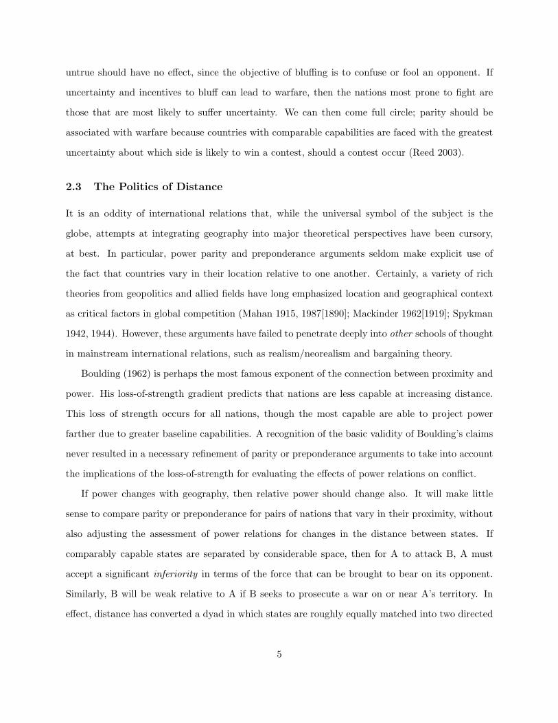
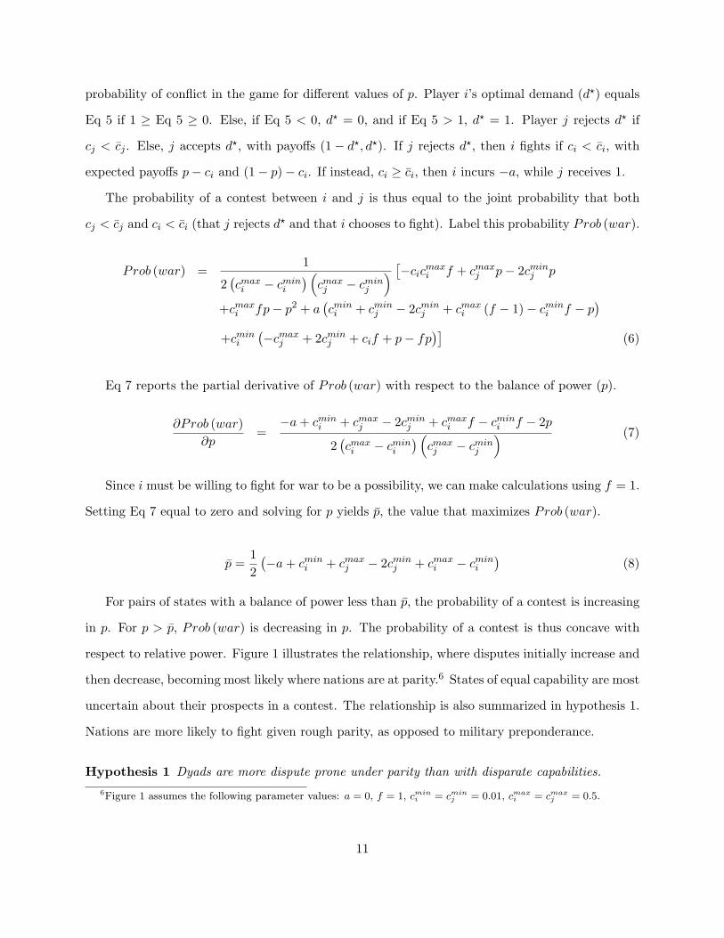
For pairs of states with a balance of power less than p̄, the probability of a contest is increasing
in p. For p > p̄, Prob (war) is decreasing in p. The probability of a contest is thus concave with
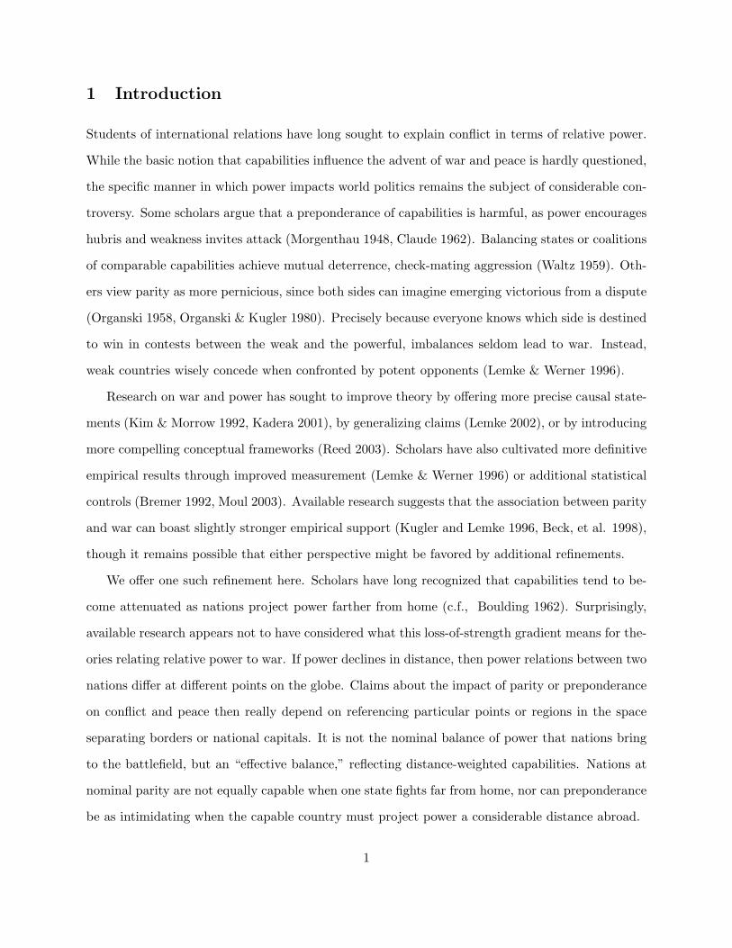
respect to relative power. Figure 1 illustrates the relationship, where disputes initially increase and
then decrease, becoming most likely where nations are at parity.6 States of equal capability are most
uncertain about their prospects in a contest. The relationship is also summarized in hypothesis 1.
Nations are more likely to fight given rough parity, as opposed to military preponderance.
Hypothesis 1 Dyads are more dispute prone under parity than with disparate capabilities.6Figure 1 assumes the following parameter values: a = 0, f = 1, cmin
i = cminj = 0.01, cmax
i = cmaxj = 0.5.
11
0 0.5 1i's capabilities �p�
0.25
0.5Prob�war�
Figure 1: Relationship between the Balance of Power and the Probability of Conflict
4.2 The Effects of Geographic Proximity
An obvious problem with the above model and prediction is that the world only weakly looks this
way. Parity is associated with an increase in conflict in many studies, but the effect is not large, nor
robust. We have suggested in our review of the literature and in the informal theoretical discussion
that this is because power is being measured without much attention to geography. The basic
model can easily be modified to capture some of the salient effects of proximity and distance.
In constructing a model of the effects of distance on the balance of power, we need to establish
an explicit functional relationship between each state’s capabilities and the probability of victory.
Contest success functions pose tradeoffs in terms of logical elegance, generality and tractability
(Hirschleifer 1995, Skaperdas 1996). Rohner (2006) offers a framework that is appealing for the
present analysis. In particular, the function is explicit, bounded in the unit interval, and differen-
tiable, allowing the game to be solved analytically. The contest success function appears below:
p =12
+ θ (ρicapi − ρjcapj) (9)
Eq 9 has several components. Each cap parameter represents the capabilities of states i and
12
j, respectively. We begin by assuming that the probability of victory for two states with equal
capabilities is 0.5. The larger θ, the more decisive the impact of advantages for either state. The
ρ parameters scale the effect of cap for each state, representing martial attributes or technology.
Once we have a way of integrating state-level attributes into the dyadic balance of power, we
can add explicit measures of the loss-of-strength that comes with distance for each country. Let us
refer again to the notion that nations are physically separated by a chord of variable distance (k).
Contests can occur anywhere along this chord. We can represent the distance from state i to any
potential dispute along the chord as z. Since fighting involves meeting, the distance from j to the
same dispute is simply the remaining length of the chord, k − z. Let effective capabilities for each
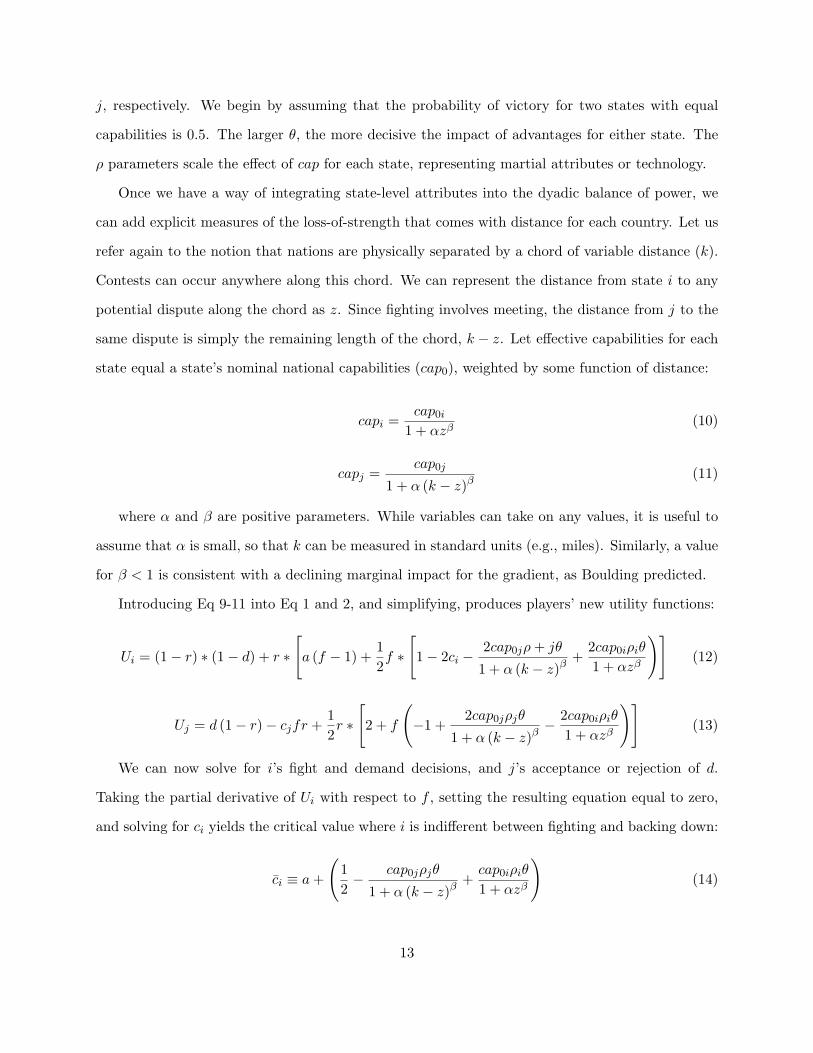
state equal a state’s nominal national capabilities (cap0), weighted by some function of distance:
capi =cap0i
1 + αzβ(10)
capj =cap0j
1 + α (k − z)β(11)
where α and β are positive parameters. While variables can take on any values, it is useful to
assume that α is small, so that k can be measured in standard units (e.g., miles). Similarly, a value
for β < 1 is consistent with a declining marginal impact for the gradient, as Boulding predicted.
Introducing Eq 9-11 into Eq 1 and 2, and simplifying, produces players’ new utility functions:
Ui = (1− r) ∗ (1− d) + r ∗
[a (f − 1) +
12f ∗
[1− 2ci −
2cap0jρ+ jθ
1 + α (k − z)β+
2cap0iρiθ
1 + αzβ
)](12)
Uj = d (1− r)− cjfr +12r ∗
[2 + f
(−1 +
2cap0jρjθ
1 + α (k − z)β− 2cap0iρiθ
1 + αzβ
)](13)
We can now solve for i’s fight and demand decisions, and j’s acceptance or rejection of d.
Taking the partial derivative of Ui with respect to f , setting the resulting equation equal to zero,
and solving for ci yields the critical value where i is indifferent between fighting and backing down:
c̄i ≡ a+
(12− cap0jρjθ
1 + α (k − z)β+cap0iρiθ
1 + αzβ
)(14)
13
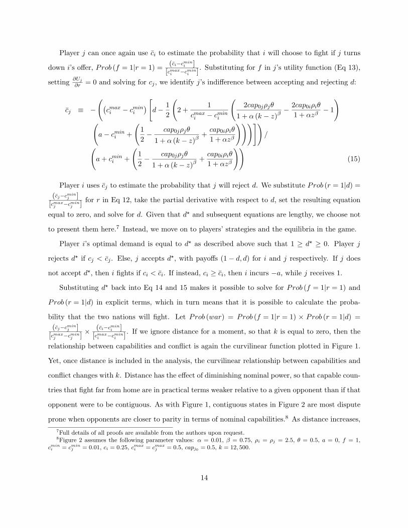
Player j can once again use c̄i to estimate the probability that i will choose to fight if j turns
down i’s offer, Prob (f = 1|r = 1) = (c̄i−cmini ]
[cmaxi −cmin
i ] . Substituting for f in j’s utility function (Eq 13),
setting ∂Uj
∂r = 0 and solving for cj , we identify j’s indifference between accepting and rejecting d:
c̄j ≡ −
((cmaxi − cmini
) [d− 1
2
(2 +
1cmaxi − cmini
(2cap0jρjθ
1 + α (k − z)β− 2cap0iρiθ
1 + αzβ− 1
)(a− cmini +
(12− cap0jρjθ
1 + α (k − z)β+cap0iρiθ
1 + αzβ
)))])/(
a+ cmini +
(12− cap0jρjθ
1 + α (k − z)β+cap0iρiθ
1 + αzβ
))(15)
Player i uses c̄j to estimate the probability that j will reject d. We substitute Prob (r = 1|d) =(c̄j−cmin
j ][cmax
j −cminj ] for r in Eq 12, take the partial derivative with respect to d, set the resulting equation
equal to zero, and solve for d. Given that d? and subsequent equations are lengthy, we choose not
to present them here.7 Instead, we move on to players’ strategies and the equilibria in the game.
Player i’s optimal demand is equal to d? as described above such that 1 ≥ d? ≥ 0. Player j
rejects d? if cj < c̄j . Else, j accepts d?, with payoffs (1− d, d) for i and j respectively. If j does
not accept d?, then i fights if ci < c̄i. If instead, ci ≥ c̄i, then i incurs −a, while j receives 1.
Substituting d? back into Eq 14 and 15 makes it possible to solve for Prob (f = 1|r = 1) and
Prob (r = 1|d) in explicit terms, which in turn means that it is possible to calculate the proba-
bility that the two nations will fight. Let Prob (war) = Prob (f = 1|r = 1) × Prob (r = 1|d) =(c̄j−cmin
j ][cmax
j −cminj ] ×
(c̄i−cmini ]
[cmaxi −cmin
i ] . If we ignore distance for a moment, so that k is equal to zero, then the
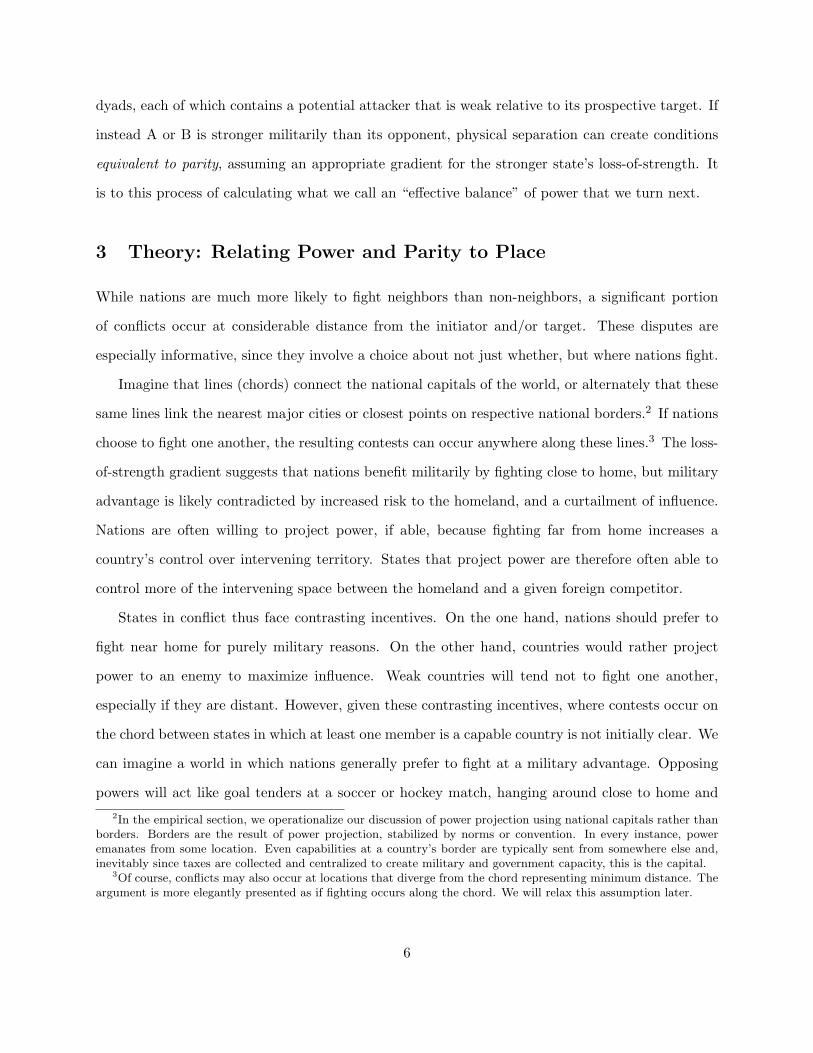
relationship between capabilities and conflict is again the curvilinear function plotted in Figure 1.
Yet, once distance is included in the analysis, the curvilinear relationship between capabilities and
conflict changes with k. Distance has the effect of diminishing nominal power, so that capable coun-
tries that fight far from home are in practical terms weaker relative to a given opponent than if that
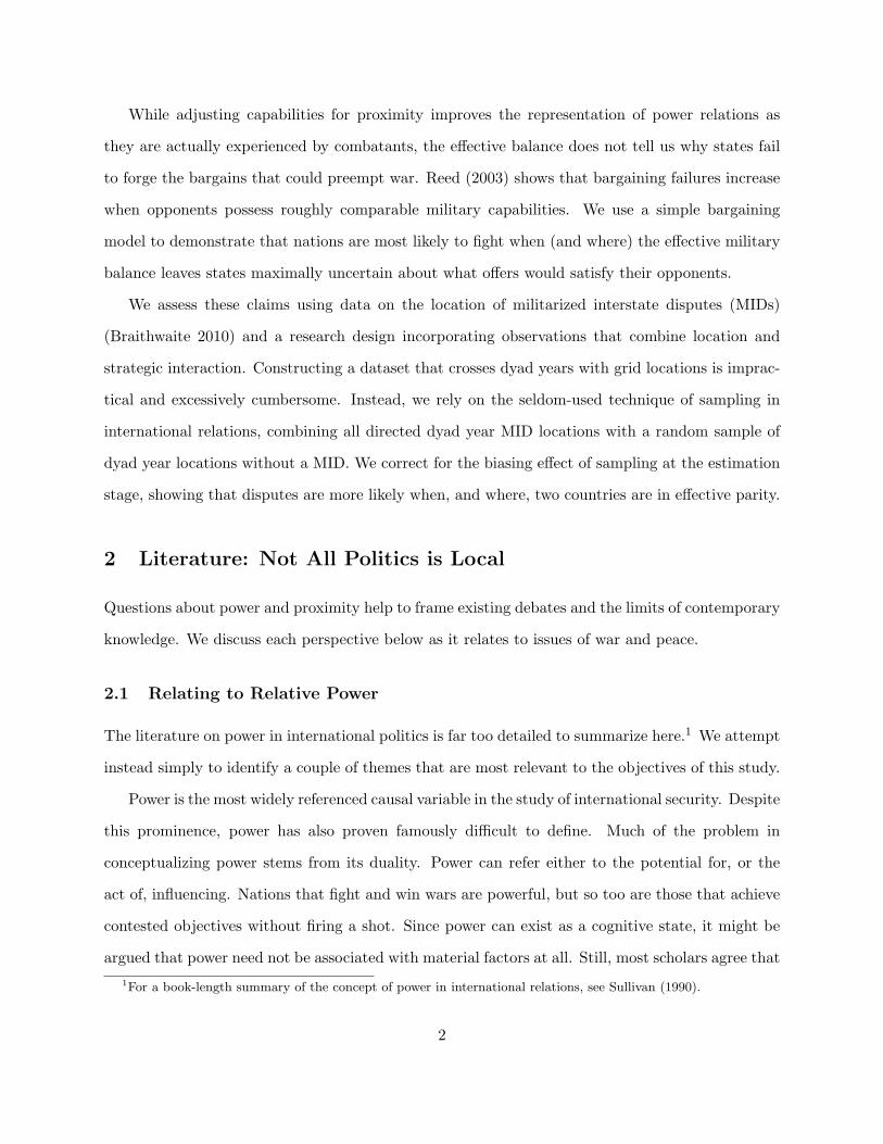
opponent were to be contiguous. As with Figure 1, contiguous states in Figure 2 are most dispute
prone when opponents are closer to parity in terms of nominal capabilities.8 As distance increases,7Full details of all proofs are available from the authors upon request.8Figure 2 assumes the following parameter values: α = 0.01, β = 0.75, ρi = ρj = 2.5, θ = 0.5, a = 0, f = 1,
cmini = cmin
j = 0.01, ci = 0.25, cmaxi = cmax
j = 0.5, capj0 = 0.5, k = 12, 500.
14
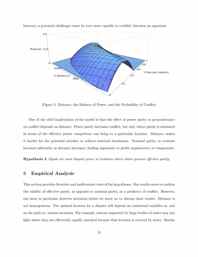
however, a potential challenger must be ever more capable to credibly threaten an opponent.
0
0.2
0.4
0.6
0.81
i's base cap. �capizero�5000
10000
i's distance �z�0
0.25
0.5
Prob�war�
Figure 2: Distance, the Balance of Power, and the Probability of Conflict
One of the chief implications of the model is that the effect of power parity or preponderance
on conflict depends on distance. Power parity increases conflict, but only where parity is measured
in terms of the effective power competitors can bring to a particular location. Distance makes
it harder for the potential attacker to achieve material dominance. Nominal parity, in contrast
becomes inferiority as distance increases, leading opponents to prefer acquiescence or compromise.
Hypothesis 2 Dyads are most dispute prone in locations where states possess effective parity.
5 Empirical Analysis
This section provides bivariate and multivariate tests of the hypotheses. Our results seem to confirm
the validity of effective parity, as opposed to nominal parity, as a predictor of conflict. However,
one issue in particular deserves attention before we move on to discuss these results. Distance is
not homogeneous. The optimal location for a dispute will depend on contextual variables at, and
on the path to, various locations. For example, nations separated by large bodies of water may not
fight where they are effectively equally matched because that location is covered by water. Similar
15
effects may result from mountain chains or other natural barriers. Conversely, economic, social or
political attributes of a given location may act as attractors, increasing or decreasing the probability
of a dispute in a given location beyond the effect of distance-weighted relative capabilities. We are
eager to explore this heterogeneity in future research. However, we view the present focus on the
effects of metric distance as a “pure play” test of the argument, one that is best suited both to
persuade an audience familiar with thinking of power relations independent of location and also
to demonstrate the basic validity of our claims. Indeed, we strongly suspect that the effect of
populating location data with relevant geo-located features will be to enhance our basic findings.
5.1 Bivariate Tests
Quantile-quantile plots are a simple tool to compare the distributions of two variables. Each
of the two figures below relates a measure of the balance of power using the COW CINC data
to the same measure where component CINC scores are weighted by the distance between the
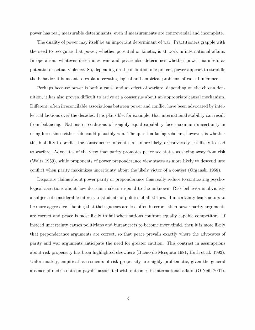
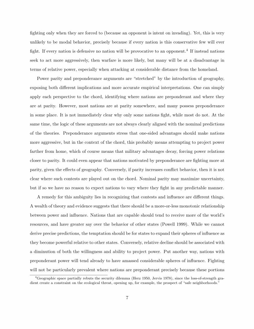
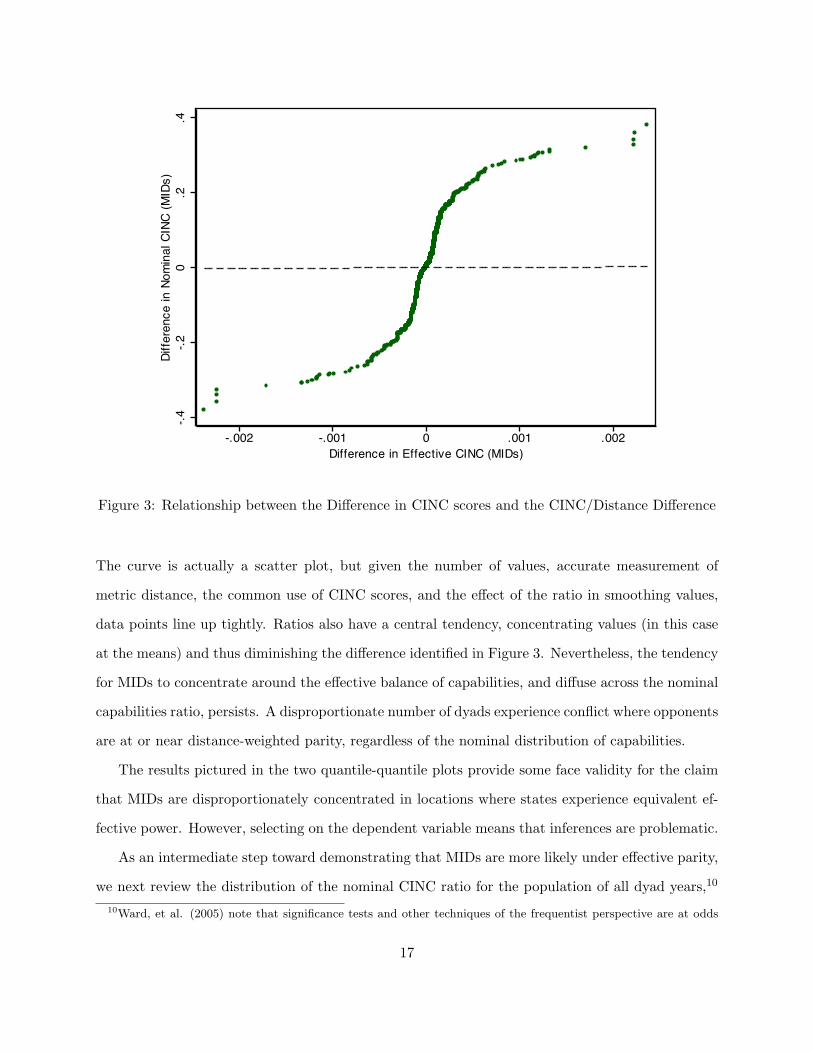
location of the dispute and the national capital. Figure 3 compares the difference in CINC scores
for states in a dispute dyad with the distance-weighted CINC difference. The relationship is non-
linear, generating an “S”-shaped (sigmoidal) curve that concentrates values of the distance-weighted
relative capabilities measure around the zero line, where both states are effectively equally matched.
In contrast, values of nominal capabilities tend to be dispersed toward the tails, where one state
has much larger nominal capabilities. If Figure 3 revealed a nearly straight diagonal line, we would
be forced to conclude that the difference in effective power and the difference in nominal power are
measuring the same thing. As it happens, the sigmoidal relationship tells us that pairs of states in
disputes are much more likely to fight where distance creates effective parity, than they are to fight
under nominal parity. Conversely, dyads show a noticeably lower propensity to fight in locations
where one nation possesses effective preponderance than to fight under nominal preponderance.
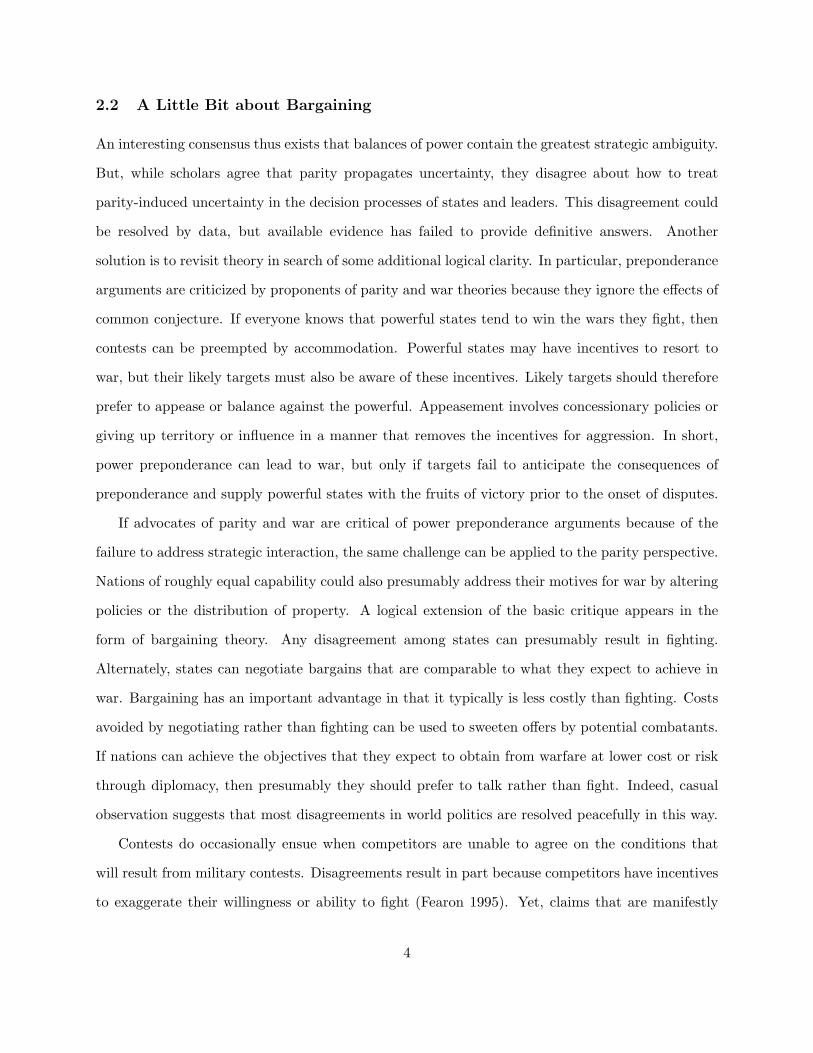
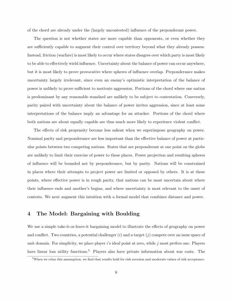
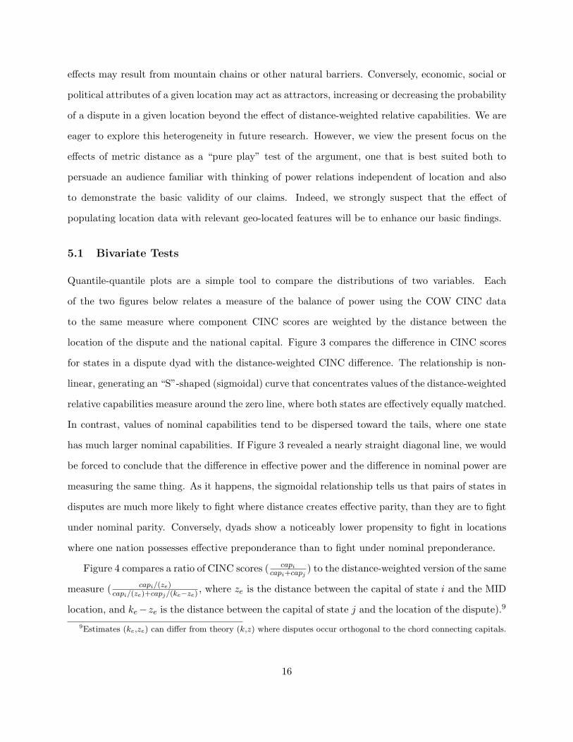
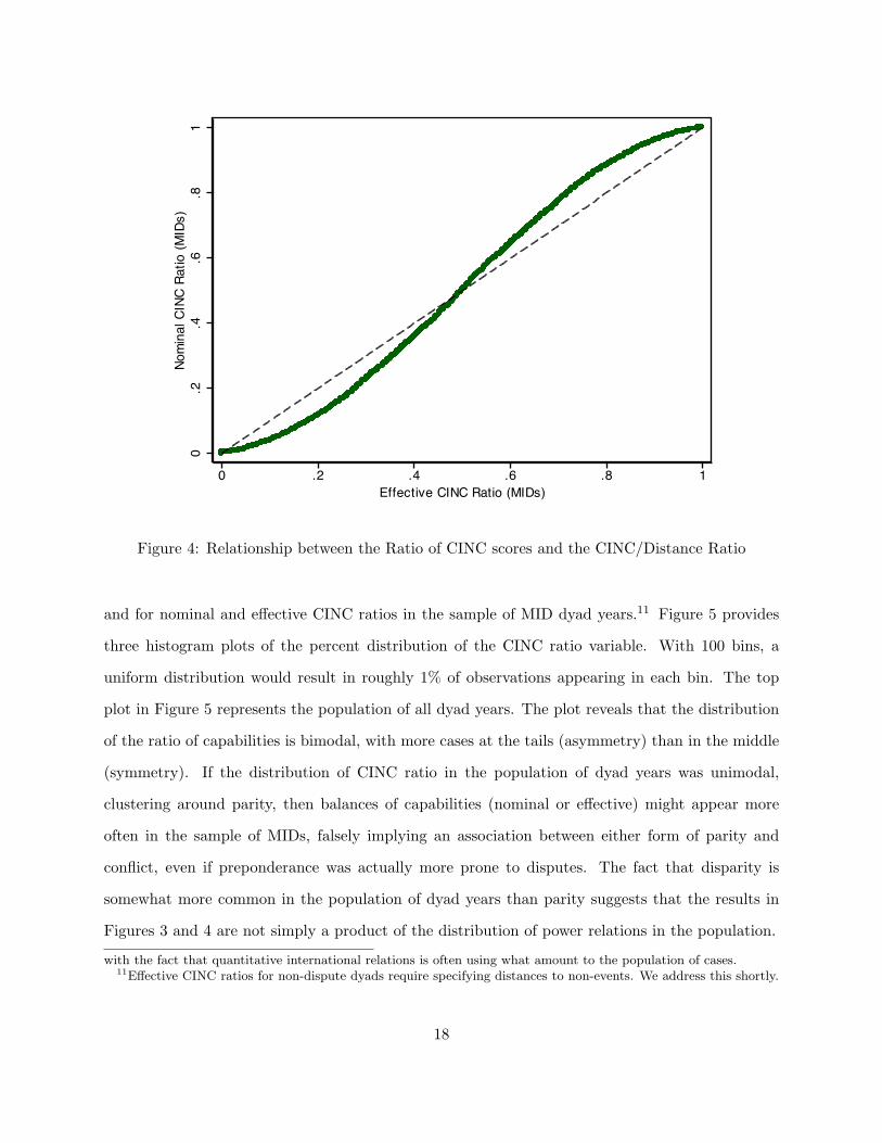
Figure 4 compares a ratio of CINC scores ( capi
capi+capj) to the distance-weighted version of the same
measure ( capi/(ze)capi/(ze)+capj/(ke−ze) , where ze is the distance between the capital of state i and the MID
location, and ke−ze is the distance between the capital of state j and the location of the dispute).9
9Estimates (ke,ze) can differ from theory (k,z) where disputes occur orthogonal to the chord connecting capitals.
16
-.4-.2
0.2
.4Di
ffere
nce
in N
omin
al C
INC
(MID
s)
-.002 -.001 0 .001 .002Difference in Effective CINC (MIDs)
Figure 3: Relationship between the Difference in CINC scores and the CINC/Distance Difference
The curve is actually a scatter plot, but given the number of values, accurate measurement of
metric distance, the common use of CINC scores, and the effect of the ratio in smoothing values,
data points line up tightly. Ratios also have a central tendency, concentrating values (in this case
at the means) and thus diminishing the difference identified in Figure 3. Nevertheless, the tendency
for MIDs to concentrate around the effective balance of capabilities, and diffuse across the nominal
capabilities ratio, persists. A disproportionate number of dyads experience conflict where opponents
are at or near distance-weighted parity, regardless of the nominal distribution of capabilities.
The results pictured in the two quantile-quantile plots provide some face validity for the claim
that MIDs are disproportionately concentrated in locations where states experience equivalent ef-
fective power. However, selecting on the dependent variable means that inferences are problematic.
As an intermediate step toward demonstrating that MIDs are more likely under effective parity,
we next review the distribution of the nominal CINC ratio for the population of all dyad years,10
10Ward, et al. (2005) note that significance tests and other techniques of the frequentist perspective are at odds
17
0.2
.4.6
.81
Nom
inal
CIN
C Ra
tio (M
IDs)
0 .2 .4 .6 .8 1Effective CINC Ratio (MIDs)
Figure 4: Relationship between the Ratio of CINC scores and the CINC/Distance Ratio
and for nominal and effective CINC ratios in the sample of MID dyad years.11 Figure 5 provides
three histogram plots of the percent distribution of the CINC ratio variable. With 100 bins, a
uniform distribution would result in roughly 1% of observations appearing in each bin. The top
plot in Figure 5 represents the population of all dyad years. The plot reveals that the distribution
of the ratio of capabilities is bimodal, with more cases at the tails (asymmetry) than in the middle
(symmetry). If the distribution of CINC ratio in the population of dyad years was unimodal,
clustering around parity, then balances of capabilities (nominal or effective) might appear more
often in the sample of MIDs, falsely implying an association between either form of parity and
conflict, even if preponderance was actually more prone to disputes. The fact that disparity is
somewhat more common in the population of dyad years than parity suggests that the results in
Figures 3 and 4 are not simply a product of the distribution of power relations in the population.
with the fact that quantitative international relations is often using what amount to the population of cases.11Effective CINC ratios for non-dispute dyads require specifying distances to non-events. We address this shortly.
18
The middle and bottom plots in Figure 5 offer histograms of the nominal and effective CINC
ratio, respectively, for the sample of militarized dispute dyad years. Note that the distributions are
progressively less bimodal, implying that dyads with nominal, and particularly effective parity are
selecting into militarized disputes more often than dyads of unequal power. This suggests that the
bivariate relationship identified in Figures 3 and 4 could be broadly accurate; pairs of states may
be most prone to fight when they are effectively at parity in terms of distance-weighted capabilities.
5.2 Multivariate Tests
Multivariate analysis allows us to stop selecting on the dependent variable even while considering
other possible causal arguments. Yet, adding “zeros” to the analysis is far from trivial. Using rough
numbers, a typical dyad year time-series–cross-section (TSCS) dataset of interstate interactions runs
to about 650,000 observations (∑k
i=1C (n, 2) =∑k
i=1n!
2!(n−2)! , where k = 2000− 1816 = 185 and n
varies between 23 and 191 depending on the number of countries in the international system). Using
directed dyads doubles this number, while including locations increases the number of observations
by at least several magnitudes of order. The PRIO GRID data used here (Tollefsen, et al. 2010)
partitions territory and ocean space into 64,804 grid cells of 0.5 decimal degrees × 0.5 decimal
degrees. In 2000, for example, the 36,342 dyads in the directed dyad year dataset must be multiplied
by 64,804 so that, in one year, the population of directed dyad year locations runs to approximately
2.355× 10⁹ observations. With all 185 years included, there are roughly 8.425× 10¹⁰ observations.
It is neither practical nor advantageous to construct datasets containing tens of billions of
observations. The obvious alternative is to sample. Yet, quantitative international relations has
shown a strong preference for including the universe of relevant cases. Randomly sampling rare
events would quickly winnow away the “ones,” ensuring that results would invariably fail to prove
statistically significant. With only 5,403 dyad year observations involving MID onsets (and 2,865
MID initiations), a manageable sample of 100, 000 cases, drawn from a population of 1 × 10¹¹
directed dyad year locations would have only about a 0.5% chance of containing even one MID.
Fortunately, a practical alternative exists in the form of non-random sampling. We include all
directed dyad year locations where a MID occurs (or is initiated), plus a randomly-drawn sample
19
of non-dispute directed dyad year locations.12 Including a hugely disproportionate number of
militarized disputes inflates estimated coefficients and artificially reduces standard errors. We then
correct for bias in the estimation stage by adjusting the ReLogit estimator for the true distribution
of positive and negative observations in the population (King & Zeng 2001a, King & Zeng 2001b)13
5.2.1 Data
The multivariate analysis relies on data from several sources. We discuss data and coding below.
Dependent Variables: The COW project Militarized Interstate Dispute dataset (MIDs) identifies
conflict events involving at least two internationally recognized states. As is conventional, we code
annualized observations of at least one MID between pairs of states (multiple MIDs are ignored).
Since subsequent-year disputes are not independently generated, we code only the first year of
conflict, examining both initiation (directional) and onset (non-directional) as dependent variables.
Capabilities: COW offers the Composite Index of National Capabilities (CINC) based on six
components: military spending and personnel, total and urban population, and iron & steel produc-
tion and energy consumption (Singer, et al. 1972, Singer 1987). These data have been widely used
elsewhere (c.f. Bueno de Mesquita & Lalman 1988, Bremer 1992, Maoz & Russett 1993). Data cov-
erage extends from 1816 to 2000 (Correlates of War Project 2005b). Controversy persists about how
best to measure power (c.f. Organski 1958, Schweller 1998), but there is no reason to believe that
these data favor our hypotheses. Indeed, given the original inspirations for, and objectives of, COW
data collection, CINC data are much more likely to favor the nominal construction of capabilities,
rather than the variant we propose here (Singer 1963; Wayman et al. 1983). To measure nominal
capabilities, we include variables for each state’s CINC score and for the dyadic interaction between
CINC scores, measured either as the difference in monadic values [Abs (CINCA − CINCB)], or
as the ratio of dyadic capabilities [ CINCACINCA−CINCB
]. Interaction terms for effective capabilities are
further constructed as follows: Abs(
CINCADistance(A,Loc)
− CINCBDistance(B,Loc)
)for the difference operational-
12Use of sampling makes it more problematic to apply or interpret various econometric techniques for addressingtemporal dependence (c.f., Beck, et al. 1998; Carter and Signorino 2007). We include a temporal count (i.e. year).
13King noted that ReLogit could be used to correct for intentional bias in a sample in a talk at the American PoliticalScience Association Conference in August, 2000. However, he was skeptical that there was a practical application ofthe technique in international relations, given huge increases in statistical computing power. Development of new,more complex units of analysis suggest that biased sampling with econometric correction may apply to many subjects.
20
ization, and[
CINCADistance(A,Loc)
/(
CINCADistance(A,Loc)
+ CINCBDistance(B,Loc)
)]for the ratio measure.
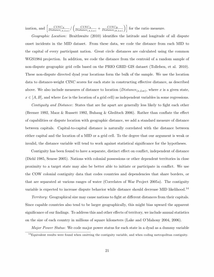
Geographic Location: Braithwaite (2010) identifies the latitude and longitude of all dispute
onset incidents in the MID dataset. From these data, we code the distance from each MID to
the capital of every participant nation. Great circle distances are calculated using the common
WGS1984 projection. In addition, we code the distance from the centroid of a random sample of
non-dispute geographic grid cells based on the PRIO GRID GIS dataset (Tollefsen, et al. 2010).
These non-dispute directed dyad year locations form the bulk of the sample. We use the location
data to distance-weight CINC scores for each state in constructing effective distance, as described
above. We also include measures of distance to location (Distance(x,Loc), where x is a given state,
x ∈ [A,B], and where Loc is the location of a grid cell) as independent variables in some regressions.
Contiguity and Distance: States that are far apart are generally less likely to fight each other
(Bremer 1992, Maoz & Russett 1992, Buhaug & Gleditsch 2006). Rather than conflate the effect
of capabilities or dispute location with geographic distance, we add a standard measure of distance
between capitals. Capital-to-capital distance is naturally correlated with the distance between
either capital and the location of a MID or a grid cell. To the degree that our argument is weak or
invalid, the distance variable will tend to work against statistical significance for the hypotheses.
Contiguity has been found to have a separate, distinct effect on conflict, independent of distance
(Diehl 1985, Senese 2005). Nations with colonial possessions or other dependent territories in close
proximity to a target state may also be better able to initiate or participate in conflict. We use
the COW colonial contiguity data that codes countries and dependencies that share borders, or
that are separated at various ranges of water (Correlates of War Project 2005a). The contiguity
variable is expected to increase dispute behavior while distance should decrease MID likelihood.14
Territory : Geographical size may cause nations to fight at different distances from their capitals.
Since capable countries also tend to be larger geographically, this might bias upward the apparent
significance of our findings. To address this and other effects of territory, we include annual statistics
on the size of each country in millions of square kilometers (Lake and O’Mahony 2004, 2006).
Major Power Status: We code major power status for each state in a dyad as a dummy variable14Equivalent results were found when omitting the contiguity variable, and when coding metropolitan contiguity.
21
where “1” is a major power according to the COW list. Since arguments for distinguishing major
powers from other states are both widely ascribed and poorly explicated, and since coding rules for
major power status in the COW data are opaque, we only include the variables in some models.
Military Alliances: Alliances are formal agreements intended to affect conflict. Alliances also
overcome distance by creating opportunities for security partners to share territory. We therefore
include a measure of the presence of an alliance in a given dyad year in some regressions, based on
the COW alliance data (Singer and Small 1966; Small and Singer 1990; Gibler and Sarkees 2004).
Democracy : Regime type is widely-used as a dimension differentiating dyadic interstate conflict
(Maoz and Russett 1993; Oneal and Russett 1999; Oneal, et al. 2003). We construct annual
democracy scores for each state as the difference between the Polity IV project’s democ and
autoc variables (Jaggers & Gurr. 1995). We further add 10 and divide the result by two for each
monad to yield the same 0-10 range as the component Polity variables. These composite Polity
scores are included in some regressions to demonstrate that our results are robust to regime type.
5.2.2 Results
The results of the multivariate analysis are presented in two tables of five regressions each. Table
1 focuses on the difference construction of nominal and effective power relations, while Table 2
examines the effects of nominal and effective power measured in terms of the ratio of capabilities.
The first regression model in Table 1 examines the nominal argument. This bare-bones model
specification includes monadic capabilities scores for each state in the dyad and the nominal differ-
ence measure, as well as variables for distance, contiguity, the year (to address trending processes
in these data) and an intercept. Each monadic CINC score is positively and significantly related to
dispute behavior, while Nominal Difference is not statistically significant. Capable states appear
(monotonically) more likely to fight. It is unclear, however, whether this is because capable states
are more dispute prone or whether they simply are better able to project power to more countries.
In addition to capabilities in the “Nominal” regression, Distance and Contiguity are negative
and significant as expected. Countries are less likely to fight as they move farther apart, if possible
in practical terms. The colonial contiguity variable ranges from 1 (“direct contiguity”) to 6 (“not
22
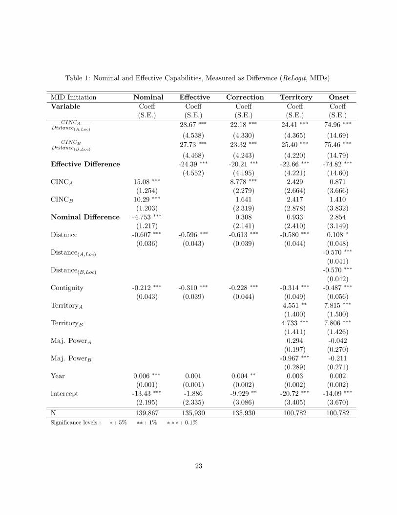
Table 1: Nominal and Effective Capabilities, Measured as Difference (ReLogit, MIDs)
MID Initiation Nominal Effective Correction Territory OnsetVariable Coeff Coeff Coeff Coeff Coeff
(S.E.) (S.E.) (S.E.) (S.E.) (S.E.)CINCA
Distance(A,Loc)28.67 ∗∗∗ 22.18 ∗∗∗ 24.41 ∗∗∗ 74.96 ∗∗∗
(4.538) (4.330) (4.365) (14.69)CINCB
Distance(B,Loc)27.73 ∗∗∗ 23.32 ∗∗∗ 25.40 ∗∗∗ 75.46 ∗∗∗
(4.468) (4.243) (4.220) (14.79)Effective Difference -24.39 ∗∗∗ -20.21 ∗∗∗ -22.66 ∗∗∗ -74.82 ∗∗∗
(4.552) (4.195) (4.221) (14.60)CINCA 15.08 ∗∗∗ 8.778 ∗∗∗ 2.429 0.871
(1.254) (2.279) (2.664) (3.666)CINCB 10.29 ∗∗∗ 1.641 2.417 1.410
(1.203) (2.319) (2.878) (3.832)Nominal Difference -4.753 ∗∗∗ 0.308 0.933 2.854
(1.217) (2.141) (2.410) (3.149)Distance -0.607 ∗∗∗ -0.596 ∗∗∗ -0.613 ∗∗∗ -0.580 ∗∗∗ 0.108 ∗
(0.036) (0.043) (0.039) (0.044) (0.048)Distance(A,Loc) -0.570 ∗∗∗
(0.041)Distance(B,Loc) -0.570 ∗∗∗
(0.042)Contiguity -0.212 ∗∗∗ -0.310 ∗∗∗ -0.228 ∗∗∗ -0.314 ∗∗∗ -0.487 ∗∗∗
(0.043) (0.039) (0.044) (0.049) (0.056)TerritoryA 4.551 ∗∗ 7.815 ∗∗∗
(1.400) (1.500)TerritoryB 4.733 ∗∗∗ 7.806 ∗∗∗
(1.411) (1.426)Maj. PowerA 0.294 -0.042
(0.197) (0.270)Maj. PowerB -0.967 ∗∗∗ -0.211
(0.289) (0.271)Year 0.006 ∗∗∗ 0.001 0.004 ∗∗ 0.003 0.002
(0.001) (0.001) (0.002) (0.002) (0.002)Intercept -13.43 ∗∗∗ -1.886 -9.929 ∗∗ -20.72 ∗∗∗ -14.09 ∗∗∗
(2.195) (2.335) (3.086) (3.405) (3.670)N 139,867 135,930 135,930 100,782 100,782Significance levels : ∗ : 5% ∗∗ : 1% ∗ ∗ ∗ : 0.1%
23
contiguous”). The higher the value of Contiguity, the lower the likelihood of a MID. Finally, Year
is positive and statistically significant, implying that disputes are more likely over time. However,
research documents that conflict propensity is dropping over time (c.f., Goldstein 2011), suggesting
misspecification. It would also be desirable to capture the variance in Year with other variables.
The second regression model in Table 1 substitutes the troika of effective capabilities measures
for the nominal power variables. Effective Difference is highly statistically significant and negative.
States are much more likely to fight in locations where effective capabilities are comparable, than
where one side or the other is at an advantage. Both monadic distance-weighted CINC scores are
positive and highly significant, again indicating that more capable states fight farther from home.
In the “Effective” regression, both geographic distance and contiguity are essentially unchanged
from the “Nominal” regression. However, the Year variable is now statistically insignificant, sug-
gesting that this model does a better job of “fitting” these data than did the previous model.
The third regression model in Table 1 allows for a direct “horse race” comparison of the nominal
and effective power variables. It is doubtful whether all six capabilities variables belong in the “true”
model. Our theoretical model suggests that effective capabilities is the critical subset, particularly
when examining the determinants of non-proximate disputes. The “Correction” model appears to
substantiate this view. The capabilities of the potential initiator remain statistically significant and
positive. However, this may again be the effect of power on opportunity, rather than on propensity.
The other two nominal variables, including the balance measure, are statistically insignificant
One concern is that these results are influenced by the physical size of states, or by other factors
reflecting international activity. The fourth model in Table 1 assesses whether the territorial size
of states actually accounts for the apparent effect of distance-weighted capabilities on militarized
disputes. While both territorial variables are positive and significant — indicating that larger
states have more MIDs — the effects of effective capabilities remain unchanged. In fact, the only
capabilities variable to become insignificant is the nominal CINC score of the potential initiator.
In addition to state size, the “Territory” regression includes dummy variables indicating monadic
major power status. Major powers are no more likely to be initiators of contests, but they are
significantly less likely to be targets of militarized disputes. However, other than the effect on
24
CINCA already mentioned, differentiating major powers from other states does little to alter the
results for the capabilities variables. Of the remaining variables, Year again becomes insignificant,
while Distance and Contiguity are largely identical to their relationships in previous regressions.
The last regression in Table 1 incorporates two changes. First, the dependent variable is dispute
onset, rather than initiation. Comparing the “Onset” regression with the other regressions helps to
show where initiation and onset produce different results, and where these results are similar. For
example, Maj. PowerB becomes statistically insignificant in this model, while it had been negative
and significant in the previous regression. Second, the regression introduces the two monadic dis-
tance to location variables. Each distance to location variable is negative and highly statistically
significant, meaning that the probability of disputes declines in the distance of the location from
either potential participant. Yet, other results are generally consistent with those reported previ-
ously. Significance levels for nominal and effective capabilities are largely unchanged, implying that
results for these variables do not depend on which actor initiates conflict. Similarly, the distance
between states and distance to location variables each appear to have distinct effects, mitigating
conflict directly, while also conditioning the impact of both relative and absolute capabilities.15
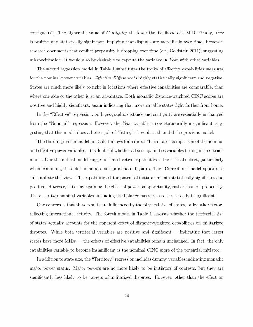
Table 2 assesses the effects of nominal and effective power relations using capabilities ratios. The
first “Linear” regression combines the monadic nominal and distance-weighted CINC scores with
a single dyadic CINC ratio for each capabilities category. Distance and Contiguity also appear in
each regression in Table 2 and operate as discussed previously. The Year variable, while included in
each regression, is never statistically significant. Finally, the two monadic territorial size variables
are always positive and significant. Larger states fight more than smaller states, ceteris paribus.
The Effective Ratio variable in the Linear model in Table 2 is only modestly statistically sig-
nificant. Nominal Ratio is actually positive and statistically significant. According to this result,
nominal disparities of capabilities increase conflict behavior. However, this model is actually poorly
specified for the hypotheses. Values for both capabilities ratios increase monotonically in CINCA
and decrease in CINCB, so that disparities occur for both low and high values of both of these
ratio variables. If rough parity is supposed to be most dispute prone, then a single ratio variable15Distance and the two monadic distance to location variables correlate at 0.2013, 0.2033 and 0.2595 respectively.
25
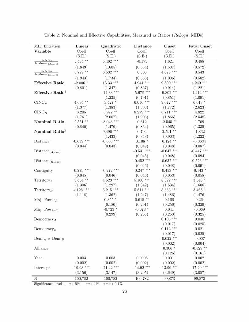
Table 2: Nominal and Effective Capabilities, Measured as Ratios (ReLogit, MIDs)
MID Initiation Linear Quadratic Distance Onset Fatal OnsetVariable Coeff Coeff Coeff Coeff Coeff
(S.E.) (S.E.) (S.E.) (S.E.) (S.E.)CINCA
Distance(A,Loc)5.434 ∗∗ 5.462 ∗∗∗ -0.175 1.621 0.488(1.849) (1.605) (0.584) (1.507) (0.572)
CINCB
Distance(B,Loc)5.729 ∗∗ 6.532 ∗∗∗ 0.305 4.078 ∗∗∗ 0.543(1.943) (1.734) (0.556) (1.006) (0.582)
Effective Ratio -2.006 ∗ 13.33 ∗∗∗ 4.944 ∗∗∗ 9.800 ∗∗∗ 4.249 ∗∗∗
(0.801) (1.347) (0.827) (0.914) (1.221)Effective Ratio2 -14.33 ∗∗∗ -5.678 ∗∗∗ -9.802 ∗∗∗ -4.212 ∗∗∗
(1.235) (0.791) (0.851) (1.091)CINCA 4.094 ∗∗ 3.427 ∗ 6.056 ∗∗∗ 9.072 ∗∗∗ 6.013 ∗
(1.377) (1.383) (1.308) (1.772) (2.623)CINCB 3.205 5.977 ∗∗ 8.279 ∗∗∗ 8.711 ∗∗∗ 4.822
(1.761) (2.007) (1.903) (1.866) (2.548)Nominal Ratio 2.551 ∗∗ -8.043 ∗∗∗ 0.612 -2.545 ∗∗ 1.709
(0.840) (1.479) (0.864) (0.965) (1.335)Nominal Ratio2 9.496 ∗∗∗ 0.704 2.591 ∗∗ -1.832
(1.433) (0.848) (0.903) (1.222)Distance -0.639 ∗∗∗ -0.603 ∗∗∗ 0.108 ∗ 0.124 ∗∗ -0.0634
(0.044) (0.043) (0.049) (0.048) (0.087)Distance(A,Loc) -0.531 ∗∗∗ -0.647 ∗∗∗ -0.447 ∗∗∗
(0.045) (0.048) (0.094)Distance(B,Loc) -0.452 ∗∗∗ -0.632 ∗∗∗ -0.526 ∗∗∗
(0.046) (0.048) (0.091)Contiguity -0.279 ∗∗∗ -0.272 ∗∗∗ -0.247 ∗∗∗ -0.453 ∗∗∗ -0.142 ∗
(0.045) (0.046) (0.046) (0.053) (0.058)TerritoryA 3.654 ∗∗ 4.523 ∗∗∗ 5.100 ∗∗∗ 8.322 ∗∗∗ 3.548 ∗
(1.306) (1.297) (1.342) (1.534) (1.606)TerritoryB 4.125 ∗∗∗ 5.215 ∗∗∗ 5.811 ∗∗∗ 8.553 ∗∗∗ 3.468 ∗
(1.118) (1.362) (1.247) (1.486) (1.476)Maj. PowerA 0.355 ∗ 0.615 ∗∗ 0.166 -0.264
(0.180) (0.201) (0.256) (0.329)Maj. PowerB -0.723 ∗ -0.673 ∗ 0.041 -0.069
(0.299) (0.265) (0.253) (0.325)DemocracyA 0.105 ∗∗∗ 0.030
(0.017) (0.025)DemocracyB 0.112 ∗∗∗ 0.021
(0.017) (0.025)Dem.A × Dem.B -0.022 ∗∗∗ -0.007
(0.002) (0.004)Alliance 0.306 ∗ -0.529 ∗∗
(0.126) (0.161)Year 0.003 0.003 0.0006 0.001 0.002
(0.002) (0.002) (0.002) (0.002) (0.002)Intercept -19.93 ∗∗∗ -21.42 ∗∗∗ -14.92 ∗∗∗ -13.99 ∗∗∗ -17.20 ∗∗∗
(3.156) (3.147) (3.295) (3.649) (3.057)N 100,782 100,782 100,782 99,873 99,873Significance levels : ∗ : 5% ∗∗ : 1% ∗ ∗ ∗ : 0.1%
26
cannot capture the curvilinear relationship between capabilities and dispute initiation or onset.
The second model in Table 2 adds a second, exponential variable for each of the nominal and
effective capabilities ratios. The combination of linear and quadratic terms best characterizes the
curvilinear relationship between the ratio of capabilities and conflict anticipated in the hypotheses.
Both Effective Ratio variables are highly significant in the anticipated directions in this “Quadratic”
regression. The probability of disputes first increases and then declines in the effective capabilities
ratio in the dyad, reflecting the central maxima predicted by hypothesis 2. The Nominal Ratio
variables are also highly statistically significant in opposite directions. However, the functional form
of the relationship is the opposite of that predicted by hypothesis 1, with a central minima rather
than a maxima. Either the parity argument is wrong for nominal capabilities — and disparity is
associated with conflict — or the Nominal Ratio variables are capturing some other dynamic.
A likely candidate as a confounding element is precisely the effects of distance incorporated into
the effective power variables. To see if this is so, the third regression (“Distance”) adds the two
monadic distance to location variables. Each is again negative and highly statistically significant.
As we speculated, controlling for the direct effects of location in the regression leads both Nominal
Ratio variables to become statistically insignificant, while the Effective Ratio variables remain
highly significant in the anticipated directions. In addition, the monadic effective capabilities
variables become statistically insignificant, while the monadic nominal capabilities variables (CINC)
remain positive and significant. Distance-weighting capabilities does not offer a unique contribution
to dispute initiation, beyond the impact of the component variables (i.e. CINCx and Distancex,Loc).
This is not problematic for our theory, which focuses on the effect of balances or imbalances
of power, but further inquiry is needed to explain why CINCxDistance(x,Loc)
perform well when relative
power is measured as difference, but not when using ratios of capabilities. Third, surprisingly,
Distance becomes positive and moderately significant when the two distance to location variables
are added to the third regression. This makes sense, however, when one realizes that capital-to-
capital distance is then measuring the effect on disputes of differences between the three distances.
Contests are less likely as the distance to location variables are large relative to the great circle
distance between national capitals. In other words, countries show a mutual preference for fighting
27
at locations that minimize the distance between their respective centers of power. The probability
of a dispute thus rises as Distance increases relative to the size of the two location distance variables.
The last two regressions in Table 2 evaluate the determinants of MID onsets and fatal MID
onsets, respectively. There are several changes to key variables using this broader measure of
conflict, but overall trends identified previously prevail. The Effective Ratio variables are the only
measures of capabilities that are consistently and highly statistically significant in the direction
predicted by our hypotheses. Lower statistical significance for the CINC score variables in the
“Fatal Onset” regression could be due either to the reduced salience of nominal monadic power when
dealing with more serious contests, or to the much lower overall likelihood of fatal disputes. Both
Nominal Ratio variables are marginally significant in the “Onset” regression. This result is most
likely a consequence of more broadly defining the dependent variable (more 1’s). Alliances should
influence conflict behavior, though standard measures of alliance status are often insignificant in
large-sample statistical studies. Interestingly, the Alliance dummy changes signs and is negatively
and significantly related to fatal MID onset, indicating that allies are less likely to experience fatal
conflict, once effective power is taken into account. In the all disputes sample, but not for fatal
MIDs, democracy demonstrates a familiar pattern in which democratic dyads are significantly less
dispute prone, while monadically democracy appears actually to increase conflict behavior.
Before concluding, it will help to verify the key relationship graphically. Figure 6 details the
effect of effective capabilities on conflict, based on the “Onset” model in Table 2. The x (horizontal)
axis contains values of the linear variable in percentiles, while the y (vertical) axis lists the combined
effect of the linear and quadratic Effective Ratio variables on the probability of MID onset. The
solid black line represents the estimated relationship, with dashed lines above and below the solid
line delineating 95% confidence intervals. With the exception of the Effective Ratio variables, all
other variables are held at their median values. As the plot shows, disputes are most likely where the
distance weighted capability ratios of states are roughly at parity (and least likely with disparity).
28
6 Conclusion
It is entirely intuitive that power influences interstate conflict, but the more precise nature of
these relationships has remained far from clear. This study offers a refinement of the basic logic
connecting parity with conflict. Parity means different nominal balances of power in different
places. Our notion of an effective balance of power reflects the implications of geography intersecting
international politics. Our analysis suggests that this is a useful distinction; effective parity appears
to be a much more effective predictor of dispute behavior than does the nominal balance of power.
Nations are most prone to fight when (and where) they are maximally uncertain about the
balance of military capabilities. Conceptualizing and operationalizing the location of contests helps
to validate this basic insight about power, uncertainty and warfare, even as it brings into focus the
need to incorporate geography as a critical component of the strategic interaction of competing
states and other actors. Students of international relations are of course aware of geography. It
is extremely difficult to discuss history, policy, or current events without introducing elements of
place as critical context. However, theories of conflict in international relations have not always paid
much attention to the role of proximity in conditioning variables such as power. As a community,
we have often allowed themselves to maintain the fiction that place could be introduced as an
afterthought, as a “control variable” in the processes leading to war and peace. We are by no
means innovative in suggesting otherwise, but perhaps claim to have found some evidence that
proximity and location are integral to both the theory and practice of international conflict.
Much remains to be done. Our conception of location is certainly minimalistic. We have
ignored almost all salient distinctions among locations; grid cells could for example include water
or mountains, or they may be the flat and grassy plains best suited to modern warfare. Obviously,
militarized disputes are more likely to occur in some locations than others because of what is on
or in those locations. Other scholars have begun to explore these issues, particularly as they relate
to civil or intra-state conflict. The analysis also glosses over a number of interesting or confusing
findings that deserve additional attention. Time and effort will hopefully remedy these omissions.
We hope that this study helps to propel the long-standing dialogue between students of politics
and geography, and thereby to improve our collective understanding of the science of peace.
29
References
Beck, Neal, Jonathan Katz & Richard Tucker. 1998. “Taking Time Seriously: Time-series–Cross-section Analysis with a Binary Dependent Variable.” American Journal of Political Science42(4):1260–1288.
Boulding, Kenneth. 1962. Conflict and Defense. New York: Harper & Row.
Braithwaite, Alex. 2010. “MIDLOC: Introducing the Militarized Interstate Dispute LocationDataset.” Journal of Peace Research 47(1):91–98.
Bremer, Stuart. 1992. “Dangerous Dyads: Conditions Affecting the Likelihood of Interstate War.”Journal of Conflict Resolution 36(2):309–341.
Bueno de Mesquita, Bruce. 1981. The War Trap. New Haven: Yale University Press.
Bueno de Mesquita, Bruce & David Lalman. 1988. “Empirical Support for Systemic and DyadicExplanations of International Conflict.” World Politics 41(1):1–20.
Buhaug, Halvard & Nils Petter Gleditsch. 2006. The Death of Distance?: The Globalization ofArmed Conflict. In Territoriality and Conflict in an Era of Globalization, ed. Miles Kahler &Barbara Walter. Cambridge: Cambridge University Press.
Carter, David B. & Curtis S. Signorino. 2007. “B to the Future: Modeling Time Dependence inBinary Data.” University of Rochester. Typescript.
Claude, Inis L. 1962. Power and International Relations. New York: Random House.
Correlates of War Project. 2005a. “Colonial/Dependency Contiguity Data, 1816-2002, version 3.0.”url: http://correlatesofwar.org.
Correlates of War Project. 2005b. “National Material Capabilities Data Documentation, version3.0.” url: http://cow2.la.psu.edu/.
Diehl, Paul. 1985. “Contiguity and Military Escalation in Major Power Rivalries, 1816–1980.”Journal of Politics 47(4):1203–1211.
Fearon, James D. 1995. “Rationalist Explanations for War.” International Organization 49(3):379–414.
Gibler, Douglas & Meredith Reid Sarkees. 2004. “Measuring Alliances: The Correlates of WarFormal Interstate Alliance Dataset, 1816–2000.” Journal of Peace Research 41(2):211–222.
Goldstein, Joshua S. 2011. Winning the War on War: The Decline of Armed Conflict Worldwide.New York: Dutton.
Herz, John. 1950. “Idealist Internationalism and the Security Dilemma.” World Politics 2(2):157–180.
Hirschleifer, Jack. 1995. “Anarchy and Its Breakdown.” Journal of Political Economy 103:26–52.
30
Huth, Paul K., D. Scott Bennett & Christopher Gelpi. 1992. “System Uncertainty, Risk Propensity,and International Conflict among the Great Powers.” Journal of Conflict Resolution 36(3):478–517.
Jaggers, Keith & Ted R. Gurr. 1995. “Transitions to Democracy: Tracking Democracy’s ‘ThirdWave’ with the Polity III Data.” Journal of Peace Research 32(4):469–482.
Jervis, Robert. 1978. “Cooperation Under the Security Dilemma.” World Politics 30(2):167–214.
Kadera, Kelly. 2001. The Power-Conflict Story: A Dynamic Model of Interstate Rivalry. AnnArbor, MI: University of Michigan Press.
Kim, Woosang & James Morrow. 1992. “When Do Power Shifts Lead to War?” American Journalof Political Science 36(4):896–922.
King, Gary & Langche Zeng. 2001a. “Explaining Rare Events in International Relations.” Inter-national Organization 55(3):693–715.
King, Gary & Langche Zeng. 2001b. “Logistic Regression in Rare Events Data.” Political Analysis9(2):137–163.
Kugler, Jacek & Douglas Lemke. 1996. Parity and War: Evaluations and Extensions of ‘The WarLedger’. Ann Arbor, MI: University of Michigan Press.
Lake, David & Angel O’Mahony. 2006. Territory and War: State Size and Patterns of InterstateConflict. In Territoriality and Conflict in an Era of Globalization, ed. Miles Kahler & BarbaraWalter. Cambridge: Cambridge University Press.
Lake, David & Angela O’Mahony. 2004. “The Incredible Shrinking State: Explaining the TerritorialSize of Countries.” Journal of Conflict Resolution 48(5):699–722.
Lemke, Douglas. 2002. Regions of War and Peace. Cambridge: Cambridge University Press.
Lemke, Douglas & Suzanne Werner. 1996. “Power Parity, Commitment to Change, and War.”International Studies Quarterly 40(2):235–260.
Mackinder, Halford. 1962[1919]. Democratic Ideals and Reality. Westport, CT: Greenwood.
Mahan, A.T. 1915. The Interest of America in International Conditions. Boston: Little, Brown,and Co.
Mahan, A.T. 1987[1890]. The Influence of Sea Power on History, 1660–1783. Fifth ed. New York:Dover.
Maoz, Zeev & Bruce Russett. 1992. “Alliances, Contiguity, Distance, Wealth, and Political Sta-bility: Is the Lack of Conflict Among Democracies a Statistical Artifact?” InternationalInteractions 17(3):245–268.
Maoz, Zeev & Bruce Russett. 1993. “Normative and Structural Causes of the Democratic Peace,1946-1986.” American Political Science Review 87(3):624–638.
31
Morgenthau, Hans J. 1948. Politics Among Nations: The Struggle for Power and Peace. New York:Knopf.
Moul, William. 2003. “Power Parity, Preponderance, and War between Great Powers, 1816–1989.”Journal of Conflict Resolution 47(4):468–489.
Oneal, John R. & Bruce Russett. 1999. “The Kantian Peace: The Pacific Benefits of Democracy,Interdependence, and International Organizations.” World Politics 52(1):1–37.
Oneal, John R., Bruce Russett & Michael L. Berbaum. 2003. “Causes of Peace: Democracy,Interdependence, and International Organizations.” International Studies Quarterly 47(3):371–393.
O’Neill, Barry. 2001. “Risk Aversion in International Relations Theory.” International StudiesQuarterly 45(4):617–640.
Organski, A.F.K. 1958. World Politics. New York: Knopf.
Organski, A.F.K. & Jacek Kugler. 1980. The War Ledger. Chicago: University of Chicago Press.
Powell, Robert. 1999. In the Shadow of Power: States and Strategies in International Politics.Princeton, NJ: Princeton University Press.
Reed, William. 2003. “Information, Power, and War.” American Political Science Review97(4):633–641.
Rohner, Dominic. 2006. “Beach Holiday in Bali or East Timor?: Why Conflict Can Lead to Under-and Overexploitation of Natural Resources.” Economics Letters 92(1):113–117.
Schweller, Randall L. 1998. Deadly Imbalances: Tripolarity and Hitler’s Strategy of World Conquest.New York: Columbia University Press.
Senese, Paul. 2005. “Territory, Contiguity, and International Conflict: Assessing a New JointExplanation.” American Journal of Political Science 49(4):769–779.
Singer, J. David. 1963. “Inter-Nation Influence: A Formal Model.” American Political ScienceReview 57(2):420–430.
Singer, J. David. 1987. “Reconstructing the Correlates of War Dataset on Material Capabilities ofStates, 1816–1985.” International Interactions 14:115–132.
Singer, J. David & Melvin Small. 1966. “Formal Alliances, 1815–1939: A Quantitative Description.”Journal of Peace Research 3(1):1–32.
Singer, J. David, Stuart Bremer & John Stuckey. 1972. Capability Distribution, Uncertainty, andMajor Power War. In Peace, War, and Numbers., ed. Bruce M. Russett. Beverly Hills, CA:Sage pp. 19–48.
Skaperdas, Stergios. 1996. “Contest Success Functions.” Economic Theory 7:283–290.
32
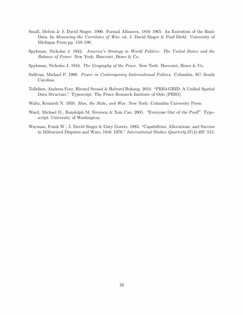
Small, Melvin & J. David Singer. 1990. Formal Alliances, 1816–1965: An Extention of the BasicData. In Measuring the Correlates of War, ed. J. David Singer & Paul Diehl. University ofMichigan Press pp. 159–190.
Spykman, Nicholas J. 1942. America’s Strategy in World Politics: The United States and theBalance of Power. New York: Harcourt, Brace & Co.
Spykman, Nicholas J. 1944. The Geography of the Peace. New York: Harcourt, Brace & Co.
Sullivan, Michael P. 1990. Power in Contemporary Iinternational Politics. Columbia, SC: SouthCarolina.
Tollefsen, Andreas Forø, H̊avard Strand & Halvard Buhaug. 2010. “PRIO-GRID: A Unified SpatialData Structure.” Typescript. The Peace Research Institute of Oslo (PRIO).
Waltz, Kenneth N. 1959. Man, the State, and War. New York: Columbia University Press.
Ward, Michael D., Randolph M. Siverson & Xun Cao. 2005. “Everyone Out of the Pool!” Type-script. University of Washington.
Wayman, Frank W., J. David Singer & Gary Goertz. 1983. “Capabilities, Allocations, and Successin Militarized Disputes and Wars, 1816–1976.” International Studies Quarterly 27(4):497–515.
33
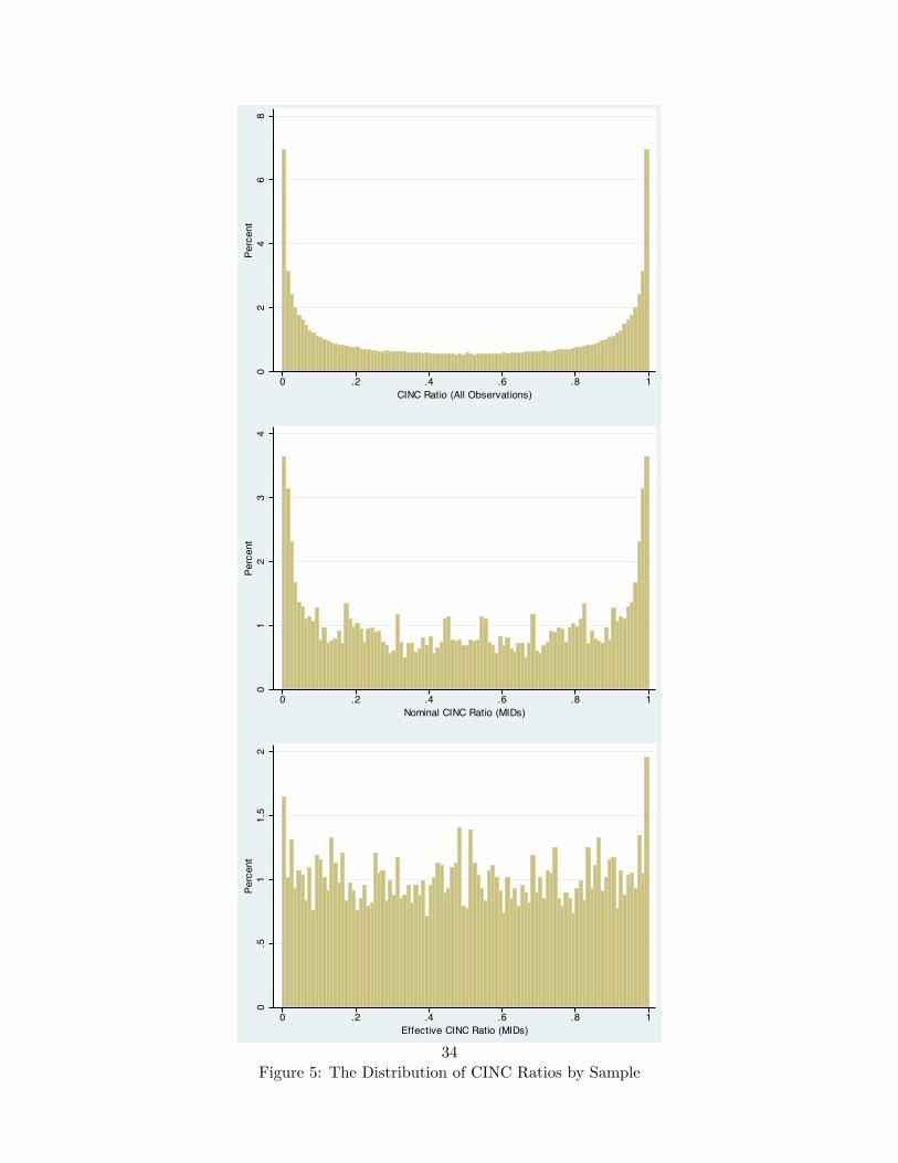
02
46
8Pe
rcen
t
0 .2 .4 .6 .8 1CINC Ratio (All Observations)
01
23
4Pe
rcen
t
0 .2 .4 .6 .8 1Nominal CINC Ratio (MIDs)
0.5
11.
52
Perc
ent
0 .2 .4 .6 .8 1Effective CINC Ratio (MIDs)
Figure 5: The Distribution of CINC Ratios by Sample34
0.0
002
.000
4.0
006
New
MID
ons
ets
(Dire
cted
Dya
ds)
0 20 40 60 80 100Effective Difference in Capabilities: percentiles from lowest to highest
Figure 6: The Effect of the Effective Ratio of Capabilities on the Probability of MID Onset
35