Power Forecast 2019: Williston Basin Oil and Gas Related ... Forecast 2019.pdf · 234 West Century Avenue Bismarck, ND 58503 701.255.5460 Power Forecast 2019: Williston Basin Oil

234 West Century Avenue

Bismarck, ND 58503

701.255.5460

www.barr.com

Power Forecast 2019: Williston Basin Oil and Gas

Related Electrical Load Growth Forecast

North Dakota

Prepared for

North Dakota Transmission Authority

May 2019

i

Power Forecast 2019:

Williston Basin Oil and Gas Related Electrical Load Growth Forecast

May 2019

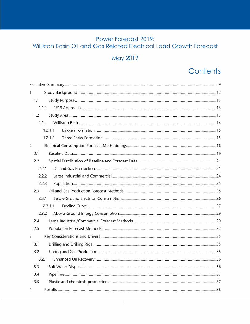
Contents

Executive Summary .............................................................................................................................................................................. 9

1 Study Background .............................................................................................................................................................12

1.1 Study Purpose ................................................................................................................................................................13

1.1.1 PF19 Approach .........................................................................................................................................................13

1.2 Study Area .......................................................................................................................................................................13

1.2.1 Williston Basin ...........................................................................................................................................................14

1.2.1.1 Bakken Formation .........................................................................................................................................15

1.2.1.2 Three Forks Formation ................................................................................................................................15

2 Electrical Consumption Forecast Methodology.....................................................................................................16

2.1 Baseline Data ..................................................................................................................................................................19

2.2 Spatial Distribution of Baseline and Forecast Data .........................................................................................21

2.2.1 Oil and Gas Production .........................................................................................................................................21

2.2.2 Large Industrial and Commercial ......................................................................................................................24

2.2.3 Population ..................................................................................................................................................................25

2.3 Oil and Gas Production Forecast Methods .........................................................................................................25

2.3.1 Below-Ground Electrical Consumption ...........................................................................................................26

2.3.1.1 Decline Curve ..................................................................................................................................................27

2.3.2 Above-Ground Energy Consumption ..............................................................................................................29

2.4 Large Industrial/Commercial Forecast Methods ..............................................................................................29

2.5 Population Forecast Methods ..................................................................................................................................32

3 Key Considerations and Drivers ...................................................................................................................................35

3.1 Drilling and Drilling Rigs ............................................................................................................................................35

3.2 Flaring and Gas Production ......................................................................................................................................35

3.2.1 Enhanced Oil Recovery ..........................................................................................................................................36

3.3 Salt Water Disposal ......................................................................................................................................................36

3.4 Pipelines ...........................................................................................................................................................................37

3.5 Plastic and chemicals production ...........................................................................................................................37

4 Results ....................................................................................................................................................................................38

Power Forecast 2019

May 2019 ii

4.1 Specific Results per Broad Load Category ..........................................................................................................39

4.1.1 Oil and Gas Production .........................................................................................................................................41

4.1.2 Large Industrial and Commercial ......................................................................................................................44

4.1.3 Population ..................................................................................................................................................................47

5 References ............................................................................................................................................................................51

Power Forecast 2019

May 2019 iii

List of Tables

Table 2-1 Baseline (2018) Energy Consumption Per-County .............................................................................. 20

Table 2-2 New Gas Processing Capacity by Year ..................................................................................................... 24

Table 2-3 Data Used to Estimate Below-Ground Energy Consumption for Oil and Gas

Production .......................................................................................................................................................... 28

Table 2-4 Data Used to Estimate Above-Ground Energy Consumption for Oil and Gas

Production .......................................................................................................................................................... 29

Table 2-5 Data Used to Estimate Large Industrial/Commercial Energy Consumption ............................. 31

Table 2-6 Data Used to Estimate Population-Based Energy Consumption .................................................. 34

Table 4-1 Study Area Forecasted Electrical Energy Consumption by Broad Load Category ................. 41

Table 4-2 Consensus Scenario: Study Area Forecasted Electrical Energy Consumption by Broad

Load Category ................................................................................................................................................... 41

Table 4-3 Low Scenario: Relative Per-County Forecasted Electrical Energy Use Associated with

Oil and Gas Production .................................................................................................................................. 43

Table 4-4 Consensus Scenario: Relative Per-County Forecasted Electrical Energy Use Associated

with Oil and Gas Production ........................................................................................................................ 44


Large Industrial and Commercial Sources .............................................................................................. 46


with Large Industrial and Commercial Sources .................................................................................... 47


Population ........................................................................................................................................................... 49


with Population ................................................................................................................................................. 50

Power Forecast 2019

May 2019 iv

List of Figures

Figure 1-1 Study Area and Associated Williston Basin Formations ................................................................... 14

Figure 2-1 GIS Database Model Inputs ......................................................................................................................... 17

Figure 2-2 NDPA Forecast: Oil Production Volumes ................................................................................................ 18

Figure 2-3 NDPA Forecast: Gas Production Volumes .............................................................................................. 18

Figure 2-4 Baseline (2018) Electrical Energy Consumption Distribution by Broad Load Category ....... 20

Figure 2-5 Oil Production (barrels/square mile) Spatial Distribution, 2023 .................................................... 23



Figure 2-8 Annual Oil and Gas Energy Consumption Forecast Process ........................................................... 25

Figure 2-9 Production Decline Curve for Dunn County .......................................................................................... 28

Figure 2-10 Baseline Population by County ................................................................................................................... 33

Figure 4-1 Study Area Forecasted Electrical Energy Consumption .................................................................... 38

Figure 4-2 Low Scenario: Study Area Forecasted Electrical Energy Consumption by Broad Load

Category .............................................................................................................................................................. 40

Figure 4-3 Consensus Scenario: Study Area Forecasted Electrical Energy Consumption by Broad Load

Category .............................................................................................................................................................. 40

Figure 4-4 Oil and Gas Production Forecasted Electrical Energy Consumption ........................................... 42

Figure 4-5 Large Industrial and Commercial Sources Forecasted Electrical Energy Consumption ....... 45

Figure 4-6 Population Forecasted Electrical Energy Consumption .................................................................... 48

List of Large Figures

Large Figure 1 Baseline Electrical Energy Consumption: 2018

Large Figure 2 Large Industrial/Commercial Sources Assumed Within PF19

Large Figure 3 Estimated Electrical Energy Consumption: 2022



List of Appendices

Appendix A Large Figures

Appendix B Formulae used in Calculations

Appendix C PF19 Sensitivities Analysis Memorandum

Appendix D NDSU Population Forecasts

Power Forecast 2019

May 2019 v

Abbreviations

bbl barrel

bpd barrels per day

BEPC Basin Electric Power Cooperative

EERC Energy & Environment Research Center, University of North Dakota

EIA Energy Information Administration, U.S. Department of Energy

ESP Electrical Submersible Pump

Esri Environmental Systems Research Institute

GIS geographic information system

MMscf/d million standard cubic feet per day

kW kilowatt

kWh kilowatt hour

MDU Montana-Dakota Utilities

MW megawatt

MWh megawatt hour

MWd megawatt day

GW gigawatt

GWh gigawatt hour

NDIC North Dakota Industrial Commission

NDPA North Dakota Pipeline Association

NDTA North Dakota Transmission Authority

NDSU North Dakota State University

NGL Natural Gas Liquid

PF12 Power Forecast 2012: Williston Basin Oil and Gas Related Electrical Load Growth Forecast

PF19 Power Forecast 2019: Williston Basin Oil and Gas Related Electrical Load Growth Forecast

psig pounds per square inch gage

SWD saltwater disposal

Power Forecast 2019

May 2019 vi

Definitions

Barrel: A barrel equals 42 US gallons.

Condensate: Also called natural-gas condensate or natural gas liquids, is a low-density mixture of

hydrocarbons that are present as gaseous components in the raw natural gas produced from many

natural gas fields, and which condense out of the gas when the temperature is reduced.

Consensus scenario: This is one of two forecast scenarios within the PF19. The consensus scenario

correlates to the NDPA’s Case 1 oil and gas production volume forecasts and NDSU’s mid oil price

scenario’s population forecast. The consensus scenario reflects higher potential for growth than the PF19’s

low scenario.

Electric power: The instantaneous rate at which electrical energy is delivered. For example one

horsepower is 550 foot-pounds force per second. Electric power is generally reported in watts, kilowatts

(kW) or megawatts (MW). For example, a natural gas processing plant might require 50 MW of power to

process gas at a rate of 350 million cubic feet per day.

Electrical energy: A measure of electricity that can accomplish a particular amount of work. Common

units of electrical energy are kilowatt hours (kWh) or megawatt hours (MWh). For example, a natural gas

processing plant might require 100 MWh of energy to process 300 million cubic feet of gas.

Electrical energy consumption: This term is used within the PF19 to describe the total electrical energy

(in MWh or GWh) used within one or more calendar years.

Energy load categories: This is the term used to describe the three categories used in the PF19 to

allocate baseline data and forecasted electrical consumption: oil and gas production, large industrial and

commercial, and population.

Fractionation: Y-grade NGL contains varying amounts of ethane, propane, butane, pentane, and heavier

hydrocarbons (referred to as C6+). NGL fractionation is the process of separating each constituent into a

purified stream, each of which has a different end use.

Gas Oil Ratio: The ratio of the volume of associated gas produced to the volume of oil produced, or

thousand standard cubic feet of gas/barrels of oil.

Gas Processing: The operation of removing natural gas liquids (NGL), water, and sulfur from associated

gas to produce a pipeline-quality natural gas product and fractionated or unfractionated NGLs.

Low scenario: This is one of two forecast scenarios within the PF19. The low scenario correlates to the

NDPA’s Case 2 oil and gas production volume forecasts and NDSU’s low oil price scenario population

forecast. The low scenario reflects lower potential for growth than the PF19’s consensus scenario.

Oil Field: A designated geographic area from which oil is produced.

Power Forecast 2019

May 2019 vii

Oil and gas load category: This is one of three energy load categories within the PF19; it represents the

estimated electrical energy required to produce and transport oil and gas products and dispose of waste

water during production activities within the Williston Basin’s Bakken and Three Forks formations. The

forecasted load estimates for this class were calculated prior to the other two load categories using

formulae described in the methods.

Large industrial/commercial load category: This is one of three energy load categories within the PF19;

it represents energy uses that are typically located in a fixed geographic location. For purposes of the

PF19, the baseline data for this category includes gas processing plants, oil refineries, and oil transmission

pipeline pumps. Additional large industrial/commercial energy uses with a fixed geographic location

beyond those described in this definition are included in the population load category for purposes of the

PF19.

Population load category: This is one of three energy load categories within the PF19; it represents the

baseline total amount of electrical energy consumed in 2018 minus the oil and gas estimated load

category and the large industrial/commercial uses category. Therefore, this load category includes

residential end uses as well as some industrial and commercial uses not allocated as being directly related

to the production of oil and gas.

Produced Water: A term used in the oil industry to describe water that is produced as a byproduct along

with oil and gas.

Pump Jack: A device used in the oil industry to extract crude oil from an oil well where there is not

enough pressure in the well to force the oil to the ground surface.

Specific Power: The power required to accomplish a specific task, which must be identified. For example,

oil production specific power is the number of kW required to produce oil at the rate of 1 barrel per day.

Specific Energy: The energy required for a particular consumer (or unit mass). For example, population-

specific energy used is the number of kWh used in 1 year by a housing unit.

Submersible Pump: A pump type of which the entire pump and motor assembly is lowered below the

surface of a liquid to push it to a higher elevation.

Transload: A facility used to physically transfer product from one transportation mode or vehicle to

another.

Water-Oil Ratio: The ratio of the volume of produced water to the volume of oil produced, or barrels

water/barrels oil.

Power Forecast 2019

May 2019 viii

Report Disclaimers/Qualifying Statements

The opinions in this report are based on information and data obtained from others and relied

upon by Barr, the NDIC, and the NDTA without independent verification unless expressly noted

herein. Statements suggesting certainty of power and energy usage and demand should be read

with that in mind.

This report was prepared for the NDIC and NDTA. Any use which a third party makes of this

report is the responsibility of such third party. Such third party agrees that Barr, the NDIC, or the

NDTA are not responsible for costs or damages of any kind, if any, suffered by it or any other

third party as a result of any use of or reliance on this report.

Barr, or any of its subcontractors and the NDIC and NDTA or any person acting on its behalf, do

not:

(A) Make any warranty or representation, express or implied, with respect to the accuracy,

completeness, or usefulness of the information contained in this report, or that the use of

any information, apparatus, method, or process disclosed in this report may not infringe

privately-owned rights; or

(B) Assume any liabilities with respect to the use of, or for damages resulting from the use of,

any information, apparatus, method, or process disclosed in this report.

The views and opinions of authors expressed herein do not necessarily state or reflect those of

the NDIC or the NDTA.

Power Forecast 2019

May 2019 9

Executive Summary

The North Dakota Transmission Authority (NDTA) hired Barr Engineering Co. (Barr) to update an electrical

load forecast completed in 2012, “Power Forecast 2012: Williston Basin Oil and Gas Related Electrical Load

Growth Forecast” (PF12.) Barr’s report, “Power Forecast 2019: Williston Basin Oil and Gas Related Electrical

Load Growth Forecast” (PF19) is an update of the previous study. The PF19’s study area includes the

Williston Basin within the state of North Dakota for 2018-2038.

The PF19 uses three broad energy load categories to organize baseline (2018) and estimated future

electrical energy consumption (in MWh) totals. The three categories included:

oil and gas production,

large industrial and commercial (for the purpose of the PF19, this included users associated to oil

and gas production) and

population.

An Environmental Systems Research Institute (Esri) based geographic information system (GIS) database

model was developed to store model inputs, parameters, and results for the PF19 study. A baseline total

electrical energy consumption total was allocated to each of the three categories and then was spatially

distributed within the database model.

The PF19 estimates future electrical energy consumption growth as a function of projected oil and gas

production volumes available from the North Dakota Pipeline Authority (NDPA) (used for the oil and gas

production and large industrial and commercial broad load categories) and projected population

estimates available from North Dakota State University (NDSU) (used for the population load category).

The PF19 estimated two scenarios for total electrical energy consumption: the low scenario and the

consensus scenario. These estimates are based on NDPA’s oil and gas production case 1 and case 2

scenarios and NDSU’s estimated county populations for low and mid oil price economic scenarios. The

PF19 forecasts are limited by uncertainty surrounding future oil prices, regulations, technology

advancements, North Dakota policy, and other potential factors. A brief description of the methodologies

used to forecast each broad load category is provided below.

Oil and Gas Production Broad Load Category Forecast Method: Monthly oil and gas production for each

oil field in 2018 was annualized and distributed amongst North Dakota Industrial Council (NDIC)-defined

oil fields. Key characteristics, such as reservoir depth, formation initial pressure, and pump efficiency were

allocated or assigned to each oil field. Total energy usage for oil and gas production was compiled by

applying formulae described in the PF19 report to estimate the energy required to pump products (oil,

gas, and water) to the ground surface and the energy required to process the oil and gas and dispose of

the waste products (i.e., the energy to pump the fluids through the gathering network to a processing,

transload, or disposal site). Annual electrical energy consumption totals for the oil and gas load category

were estimated on a per-oil-field basis using the total volumes of oil, gas, and water production estimated

by NDPA.

Power Forecast 2019

May 2019 10

Large Industrial and Commercial Broad Load Category Forecast Method: The PF19’s large

industrial/commercial load category includes gas processing plants, oil refineries, and oil transmission

pipeline pumps. For gas processing plants, a specific energy consumption of 13.2 MWd for every 100

million standard cubic feet (MMscf) of gas processed was used to calculate gas processing energy. Data

provided by NDPA identify locations for some of the planned new capacity, but additional new capacity

will be required which at present is not announced and for which geographic locations have not been

identified. The additional new capacity was estimated based on gas production volumes and the

estimated geographic locations of produced gas volumes. For oil refineries, known existing and planned

refineries were included. For oil transmission pipeline pumps, the total horsepower required to move the

product through a pipeline was estimated based on capacity and diameter of the pipeline for existing

pipelines. The same methodology was used for one potential future pipeline, the Liberty Pipeline.

Population Forecast Method: Forecasted electrical energy consumption totals for the population load

category were determined based on the anticipated growth rates provided in the “Williston Basin 2016:

Employment, Population, and Housing Forecasts” study completed by NDSU. Using baseline data from

Basin Electric and Montana Dakota Utilities, Barr estimated a per capita electrical consumption rate for

each county and applied the electrical consumption to the forecasted population numbers provided in the

NDSU data.

Results: The PF19’s estimated total amount of additional electrical energy consumption required within

the study period (2018-2038) reflected an overall growth rate of approximately 44% (low scenario) to 71%

(consensus scenario). At the end of the study period (2038), the low scenario forecasts a total annual

consumption of 15,000 GWh and the consensus forecasts a total annual consumption of 18,000 GWh of

electrical energy consumption. Compared to the baseline, this represents an increase of 4,600 GWh for

the low scenario and 7,500 GWh for the consensus scenario. Consistent with the needs to meet margin

requirements, this implies an increase in generation capacity of 670 megawatts (MW) to 1,000 MW

(calculated using a 92% load factor and an 86% capacity factor) above the capacity demand.

The majority of the growth is in load categories which have nearly flat demand curves (i.e., oil and gas

production and large industrial/commercial sources related to oil and gas production), and do not readily

lend themselves to interruptible power supply. Therefore the estimated new demand will typically be

supplied by base load capacity or mid-load capacity with fast dispatch rates.

The state’s base load generating capacity, not including Heskett Station, is 4,380 MW. Since existing base

load resources in North Dakota are operating well above industry averages, new base load or equivalent

will likely be selected by utilities that need to meet this increased demand.

The total estimated energy in MWh for the low scenario and the consensus scenario is illustrated

Figure ES-1.

Power Forecast 2019

May 2019 11

Figure ES-1 Study Area Total Forecasted Electrical Consumption

Power Forecast 2019

May 2019 12

1 Study Background

The North Dakota Transmission Authority (NDTA) facilitates the development of transmission

infrastructure in North Dakota. The NDTA was established “to serve as a catalyst for new investment in

transmission by facilitating, financing, developing, and/or acquiring transmission to accommodate new

lignite and wind energy development” (reference [1]). To be successful in electrical infrastructure planning,

the NDTA wants an understanding of North Dakota’s energy capabilities and needs while considering

increases in electrical load growth due, in large part, to energy-intensive development of oil and gas

production within the Williston Basin.

In 2012, NDTA developed an electrical load forecast in this region to better understand potential future

load growth. The expected growth was anticipated to be primarily a result of oil and gas production and

secondary infrastructure and associated population growth required to support production needs. This

study, “Power Forecast 2012: Williston Basin Oil and Gas Related Electrical Load Growth Forecast” (PF12,

reference [2]), forecasted a need for an additional 2,500 MW of capacity (or approximately three times

increase over the 2012 – 2032 study period) for the PF12’s study area (which included the Williston Basin

within North Dakota, South Dakota, Montana, and Wyoming).

The PF12 considered population growth, commercial and industrial development, and primary and

secondary employment requirements resulting from the “oil boom.” Because drilling rigs were a limiting

factor for development, the count of available drilling rigs, drilling rig efficiencies, and the number of

producing wells within specific oil-producing regions were the most significant factors in the forecast. The

PF12 used projected well counts by year to build out portions of the future oil field infrastructure model;

the estimated well counts were then used to calculate demand cases for low, consensus, and high forecast

scenarios.

NDTA engaged Barr Engineering Co. (Barr) to update the forecasts in the PF12 study in 2019. This report,

“Power Forecast 2019: Williston Basin Oil and Gas Related Electrical Load Growth Forecast” (PF19),

summarizes the findings of the updated forecast for 2018 through 2038. The PF19 update is limited to

North Dakota and primarily relies on publicly available information to estimate future electrical energy

consumption for 2019 through 2038. The method of forecasting total growth was changed for the PF19

(Section 1.1.1), but the goal of estimating future load growth as a function of oil and gas development

was the same.

The PF19 uses North Dakota Pipeline Authority’s (NDPA’s) oil and gas production forecast data which is

based on projected oil prices. The PF19 also incorporates population forecast data from NDSU,

information on projected point-source loads (loads from large industrial/commercial energy consumers)

acquired from industry contacts, and publicly available information. The PF19 forecasts are limited by

uncertainty surrounding future oil prices, regulations, technology advancements, North Dakota policy, and

other potential forces. More details about the sources of information and how it is used in the PF19 is

provided in Section 2.

Power Forecast 2019

May 2019 13

1.1 Study Purpose

The purpose of the PF19 is to estimate anticipated future electrical energy consumption demands within

the state of North Dakota, primarily within the oil-producing counties, for the next 20 years. Significant

changes occurred in the region after the PF12 forecast that affect electrical load growth including but not

limited to oil price changes, technology advancement, and regulatory changes. Because of the number of

changes and differences from key assumptions in the PF12 forecast, the previous projections were

outdated. This study provides an updated estimate of electrical energy consumption growth in the region

using more recent information and updated key assumptions that affect electric load growth.

While it is understood that peak demand is important for system planning, this report does not

specifically estimate peak demand. The relationship between total energy consumption and peak demand

is highly dependent on the type of load, and the fraction of each load type on the system. To address

that, this report estimates load growth for three broad load categories and the geographic distribution of

those loads. It is expected that the individual electric utilities will have the best understanding of the

relationships between load type and capacity factor for their own systems, and will be able to use this

data to make their own projections of peak demand.

1.1.1 PF19 Approach

The PF19 estimates future electrical energy consumption growth as a function of projected oil and gas

production volumes available from NDPA. The forecast method used in PF19 differs from that used in

PF12. PF19 considers the baseline and projections for three broad load categories: oil and gas production,

large industrial/commercial uses related to processing needs of the oil and gas production, and

population (Section 2). PF19 estimates are made directly from estimated future oil and gas production

rates and the associated electrical consumption required to produce those volumes. Population growth

and large industrial/commercial projections formed the basis to calculate the related change to electrical

consumption in those categories. PF19 does not estimate future electrical energy consumption directly as

a function of well count, rig count, or many of the other variables considered in the PF12. Instead, many of

these assumptions in PF12 are now considered in oil production and population estimates from NDPA

and NDSU and are incorporated into the PF19 as a function of the NDPA and NDSU forecasts which use

many of those same factors as the PF12 for their forecasts (e.g., well counts).

Given the uncertainty of oil prices and other factors outside of Barr’s or NDTA’s control, the PF19 was

designed so it may be readily updated to account for changes driven by oil prices, increased efficiencies,

changes in production rates, or enhanced oil recovery methods. The GIS data based approach also allows

for new information, which may not be currently available, to be incorporated into future updates.

1.2 Study Area

The study area for the PF19 is smaller than the PF12 and is limited to the state of North Dakota (to serve

the needs of the NDTA). The study area is comprised of the Basin Electric Power Cooperative (BEPC) and

the MDU service areas within the Williston Basin in North Dakota. This includes the 24 western North

Dakota counties as shown in Figure 1-1.

Power Forecast 2019

May 2019 14

Figure 1-1 Study Area and Associated Williston Basin Formations

1.2.1 Williston Basin

The Williston Basin is a large geological feature centered in Williston, North Dakota; the full basin area

compromises nearly 300,000 square miles including portions of North Dakota, South Dakota, Montana,

Saskatchewan, and Manitoba (reference [3]). The formation of oil and gas within the Williston Basin was

the result of many geologic events occurring over millions of years.

The Oil and Gas Division of the North Dakota Industrial Council (NDIC) combines production statistics

within the Williston Basin for the Bakken and Three Forks formations. Over 90% of the oil and gas

production in North Dakota comes from these two formations. This report follows the NDIC convention of

Power Forecast 2019

May 2019 15

combining production data for the Bakken and Three Forks. Descriptions of the Bakken formation and the

Three Forks formation are provided in the following subsections.

1.2.1.1 Bakken Formation

The Bakken Formation (Bakken) lies within the subsurface formation of the Williston Basin; the portion of

the Bakken formation within North Dakota is illustrated in Figure 1-1. The Bakken has been the main oil-

producing formation (outside of conventional oil drilling) within the Williston Basin since its discovery. The

maximum thickness of the Bakken is 150 feet and consists of three distinct layers. The top and bottom

layers are known to have black, organic-rich shales, and the middle layer is largely composed of siltstones

and sandstones (reference [4]). This middle layer is the primary oil-producing layer of the Bakken

Formation and the focus of most current oil production efforts in North Dakota.

1.2.1.2 Three Forks Formation

Additional oil production beyond the middle stratum of the Bakken Formation within North Dakota has

largely focused on extraction from the underlying Three Forks Formation. The portion of the Three Forks

formation within North Dakota is illustrated in Figure 1-1. Throughout a large majority of the Williston

Basin, the Three Forks Formation maintains a maximum thickness of 270 feet (reference [5]). Most oil and

natural gas production has targeted the upper Three Forks Formation (first bench) consisting of layers of

carbonates and evaporates, mudstone, dolomite, and peritidal sediments (reference [6]). The middle

(second bench) and lower (third bench) Three Forks Formation are currently being assessed for future oil-

and water-saturation capacities and future development (reference [7]).

Power Forecast 2019

May 2019 16

2 Electrical Consumption Forecast Methodology

The study area’s electrical energy consumption growth is predominately influenced by the oil and gas

sector and is expected to be in the future unless certain significant developments occur. As such, the PF19

estimates future electrical consumption growth as a function of projected oil and gas production volumes

available from NDPA. This approach is based on the premise that a particular amount of energy is

required to produce a barrel of oil and an understanding that there is a correlation between oil and gas

production rates and electrical consumption. The PF19 approach also assumes that increased demands for

large industrial/commercial energy users such as gas processing plants, refineries, and oil pipelines are

correlated to increased oil and gas production. Other loads such as commercial, retail, and municipal

energy use are presumed to be more closely correlated to population growth. Additionally, while

population growth may be driven by the need for labor in the oil and gas industry, there are other factors

which may limit population growth rate. Consequently, the electrical energy consumption is divided into

three broad load categories and calculated based on data sets provided by reliable authorities which

estimate the underlying variables directly. It is recognized that other factors may also impact overall

electric load growth; however, the focus of the PF19 is on impacts to electrical energy consumption

growth associated with increased oil and gas production within the Bakken and Three Forks Formations of

the Williston Basin.

An Environmental Systems Research Institute (Esri)-based geographic information system (GIS) database

model was developed to store model inputs, parameters, and results for the PF19 study. Information

regarding the total electrical consumption in 2018 was provided by MDU and BEPC to serve as the

baseline electrical consumption totals. The 2018 electrical energy consumed (in kWh) was allocated to the

three broad energy load categories used to organize consumption within the PF19 model and to spatially

distribute the total consumption. Forecasted estimates were completed using GIS tools and Python

scripting within the Esri ArcMap© software and organized into the same three broad energy load

categories as the baseline. The following three broad load categories comprise the GIS database model as

illustrated in Figure 2-1:

1 Oil and gas production

2 Large industrial/commercial (includes gas processing plants, oil refineries, and transmission

pipeline pumps)

3 Population

Power Forecast 2019

May 2019 17

Figure 2-1 GIS Database Model Inputs

Data from various sources were used to determine how to allocate the baseline data within the three

broad energy load categories (e.g., NDIC oil field boundaries, 2018 NDPA oil and gas production volumes,

2017 U.S. Census data, and NDIC information and industry input). Several data sources were also used to

inform the forecast data and methods (e.g., NDPA forecasted oil and gas production volumes, formulae as

described throughout this report, and NDSU population forecasts). Stakeholder outreach and industry

input was gathered by NDTA and provided to Barr. Information input into the database model was

organized so that parameters with impacts on the forecasted estimates are distinctly identified and can be

easily updated and reloaded into the database model as new information becomes available.

The method used in this study forecasted total anticipated electrical energy (MWh or GWh) to be

consumed on an annual basis; electric power demand in MW or gigawatt (GW) is not reported. While

electric demand capacity is not reported, it is considered in hypothetical terms within the results section

of the report (Section 4). The PF19 estimated two scenarios for total electrical energy consumption: the

low scenario and the consensus scenario. For the oil and gas production broad load category, the PF19’s

consensus scenario corresponds with NDPA’s Case 1 Scenario for oil and gas production and the low

scenario corresponds with NDPA’s Case 2 Scenario for oil and gas production. The NDPA scenarios are

updated regularly and published to the NDPA public website and raw data was emailed to Barr [8].

Descriptions of the Case 1 and Case 2 scenarios are provided below.

Case 1 Scenario – The expected oil production scenario based on current technology and the U.S.

Department of Energy (DOE) oil price forecast. Refer to Figure 2-2 for estimated oil production

Power Forecast 2019

May 2019 18

totals. The expected gas production scenario is based on the gas oil ratio which increases as the

well ages (causing the growth rate of the gas forecast to accelerate faster than the oil forecast).

Refer to Figure 2-3 for estimated gas production totals.

Case 2 Scenario – The expected oil production scenario is based on the same DOE price forecast

as Case 1, but assumes lower industry activity in North Dakota at the forecast prices. For example,

at $75 per barrel forecast price, more activity is concentrated in Texas or other plays around the

U.S. and less oil and gas production would be expected in North Dakota. Refer to Figure 2-3 for

estimated oil production totals. The expected gas production scenario is forecasted in the same

way as it is described for the Case 1 scenario but included the modified oil production volumes.

Refer to Figure 2-3 for estimated gas production totals.

Figure 2-2 NDPA Forecast: Oil Production Volumes

Figure 2-3 NDPA Forecast: Gas Production Volumes

Power Forecast 2019

May 2019 19

The large industrial/commercial consumptive broad load category accounted for within the PF19 are also

directly related to oil and gas production as described in Section 2.4.

For the population broad load category, the PF19 assumed population growth rates included in NDSU’s

Williston Basin 2016 forecast estimates which also incorporated estimated oil and gas production volumes

into various scenarios as described in Section 2.5.

The remaining sections of the electrical consumption forecast methodology provide the following

additional details regarding methodologies used to complete the PF19:

Section 2.1 describes how the baseline MDU and BEPC 2018 electrical energy consumed (in MWh)

was distributed across the three broad energy load categories

Section 2.2 describes how baseline and forecasted data were distributed spatially

Section 2.3 provides additional details on the oil and gas production forecast method

Section 2.4 provides additional details on the large industrial/commercial forecast method

Section 2.5 provides additional details on the population forecast method

2.1 Baseline Data

BEPC and MDU provided baseline electrical consumption data (in kWh) to Barr in a format organized by

rate class; Barr allocated the rate classes to each of the three broad energy load categories used to

estimate future electrical consumption. To distribute the data across the broad load categories, Barr first

calculated the total energy consumption required to produce the volume of oil and gas produced in 2018

(Section 2.3). Barr then allocated the sources of large industrial/commercial energy consumers known to

be related to the production of oil and gas, including natural gas processing plants, oil transmission

pipeline pump stations, and oil refineries (Section 2.4). Finally, Barr allocated the remaining energy

consumed in 2018 to the population load category (Section 2.5). As such, MDU and BEPC’s rate class

categories do not directly correlate to the PF19’s three load categories. Furthermore, the PF19 study’s

distribution also results in almost half of MDU and BEPC’s 2018 commercial or industrial electric usage

being allocated to the PF19’s population load category.

The organization of the baseline data was used to confirm, calibrate, or validate the forecast methods

(Section 2.3). The baseline electrical consumption was approximately 10,500 GWh. The distribution of the

total electrical energy consumption for the three broad energy load categories is shown in Figure 2-4. The

breakdown of how the total electrical energy consumption was allocated per category is provided in

Table 2-1 and is illustrated in Large Figure 1 in Appendix A.

Power Forecast 2019

May 2019 20

Figure 2-4 Baseline (2018) Electrical Energy Consumption Distribution by Broad Load

Category

Table 2-1 Baseline (2018) Energy Consumption Per-County

County Oil and Gas Production

Broad Load Category (GWh)

Large Industrial/Commercial Usage


Population Broad Load

Category (GWh)

Adams 0 0 43

Billings 76 28 68

Bottineau 41 0 98

Bowman 154 0 20

Burke 42 0 52

Divide 66 0 26

Dunn 460 42 585

Golden Valley 8 6 145

Hettinger 0 29 126

McHenry 1 135 227

McKenzie 1065 8 357

McLean 13 0 120

Mercer 0 0 165

Mountrail 434 63 1009

Oliver 0 0 109

Pierce 0 1306 38

Renville 19 0 84

Power Forecast 2019

May 2019 21

County Oil and Gas Production


Large Industrial/Commercial Usage


Population Broad Load

Category (GWh)

Rolette 0 0 50

Sheridan 0 0 84

Slope 12 0 101

Stark 39 0 343

Ward 1 0 276

Wells 0 0 37

Williams 581 912 836

Total 3012 2530 5000

2.2 Spatial Distribution of Baseline and Forecast Data

Spatial distribution of the baseline and forecast data was completed for each broad energy load category

used in the database model. The distribution approach for each of the three broad energy load categories

is described in the following subsections.

2.2.1 Oil and Gas Production

To establish baseline conditions, oil and gas production was attributed to each oil field within the

Williston Basin based on oil field production data for 2018 provided by NDIC. The total sum of production

for all oil fields provided by the NDIC was slightly less than the total production provided for the Williston

Basin. The differences in production totals were attributed to production in confidential wells. In some

cases, oil wells may be considered “confidential” (which are typically exploratory in nature or in early

stages of development) and the NDIC data set does not identify status (oil field well or otherwise). The

difference between the total basin production and reported oil field totals were distributed proportionally

across the oil fields based on the number of confidential wells reported in each oil field at the end of

2018.

To establish forecast conditions, increases of forecasted oil and gas production provided by NDPA were

allocated to oil fields under an assumption that the areas with the highest historic production rates within

the Bakken and Three Forks Formations will see a proportionate distribution of future production. This

represents the drilling of in-fill wells in the most productive and profitable parts of the formation. In later

years, the distribution was changed so that production was more broadly distributed across the Three

Forks Tier I and Three Forks Tier II regions by increasing the amount of new production allocated to the

lower production rate areas from the baseline year by a small percentage (approximately 1% per year).

The distribution of forecasted volumes and the shift in how those forecasted volumes were distributed

assumes that the highest production rate areas will not sustain the forecasted growth throughout the

entirety of the study period. In other words, it is assumed that new production within the Williston will

geographically shift in the later years of the study period.

Power Forecast 2019

May 2019 22

The distribution was based in part on data provided by the NDPA and was also based in part on industry

input. The geographic extents of where forecasted oil and gas production will occur is unknown and

difficult to accurately estimate. However, the locations of future production impact the forecasted

estimated energy use reported by county within the PF19. To inform the oil and gas production broad

load category’s estimated electrical energy consumption forecast by county, figures illustrating the

model’s distribution of oil production are provided for 2023 (Figure 2-5), 2028 (Figure 2-6), and 2033

(Figure 2-7). The gas production distribution mirrors that of oil production.

Power Forecast 2019

May 2019 23

Figure 2-5 Oil Production (barrels/square

mile) Spatial Distribution, 2023





PF19 PF19 PF19

Power Forecast 2019

May 2019 24

2.2.2 Large Industrial and Commercial

Existing large industrial/commercial uses with distinct geographic locations (natural gas processing plants

and oil refineries) were mapped in accordance with their actual locations. Baseline oil transmission

pipeline pump station loads were calculated as a total and distributed evenly across the pipeline corridor.

Future large industrial/commercial consumers with distinct geographic locations (natural gas processing

plants and oil refineries) were placed in accordance with their planned locations if known, or were placed

based on professional judgment of likely locations. The PF19 incorporates new gas processing capacity as

a function of the requirement to meet the regulated gas capture goals and per the increased production

rates. In both the low growth scenario and the consensus scenario multiple new gas processing plants will

be required.

Barr compared the gas production volumes for four different geographic regions to the gas processing

capability in those regions to determine where new gas plants might be needed. Existing gas plant

capacity includes all plants currently operating, under construction or announced expansions as of

April 30, 2019. Table 2-2 shows the timing of new gas processing capacity which will be required for each

region, in addition to the existing capacity.

Table 2-2 New Gas Processing Capacity by Year

Region 1 Scenario 2019 or

2020

2021 or

2022

2023 or

2024

2025 or

2026

2027 or

2028

2029 or

2030

2031 or

2032

2033 or

2034

2035 or

2036

2037 or

2038

A low 0 80 0 50 0 40 0 0 0 0

A consensus 0 100 0 0 0 0 0 0 0 0

B low 0 240 0 0 120 120 60 0 60 0

B consensus 0 390 150 1500 150 150 0 150 0 0

C low 200 0 0 50 0 0 0 0 0 0

C consensus 0 0 0 0 200 0 200 0 0 0

E low 0 0 0 0 0 0 0 0 0 0

E consensus 0 20 20 20 0 20 0 0 0 0

Notes: units of gas plant capacity are in MMscf per day 1 The regions were selected to represent specific co-op territories according to the list below.

A: Burke-Divide Electric Cooperative, north Central Electric Cooperative, Sheridan Electric Cooperative

B: Lower Yellowstone Electric Cooperative, McLean Electric Cooperative, Mountrail-Williams Electric Cooperative, Verendrye Electric

Cooperative

C: McKenzie Electric Cooperative

E: Goldenwest Electric Cooperative, Roughrider Electric Cooperative, Slope Electric Cooperative

One future oil transmission pipeline was assumed (Liberty Pipeline) and a potential alignment was based

on professional judgment and understanding of the pipeline’s anticipated terminus. Estimated forecasted

electrical energy consumption for the pump stations associated to this potential future pipeline were then

distributed across the estimated pipeline corridor.

Power Forecast 2019

May 2019 25

2.2.3 Population

Population was distributed according to the U.S. Census county and incorporated areas breakdown.

Projections of future population were distributed proportionate to the baseline distribution of the

population in 2018.

2.3 Oil and Gas Production Forecast Methods

Monthly oil and gas production for each oil field in 2018 was annualized and distributed amongst NDIC-

defined oil fields. Key characteristics such as reservoir depth, formation initial pressure, and pump

efficiency were allocated or assigned to each oil field (Figure 2-8). Total electrical energy consumption for

oil and gas production was compiled by applying formulae described below to estimate the energy

required to pump products (i.e., oil, gas, and water) to the ground surface and to estimate the energy

required to process the oil and gas and dispose of the waste products (i.e., the energy to pump the fluids

through the gathering network to a processing, transload, or disposal site). Annual electrical energy

consumption totals for the oil and gas load category was estimated on a per-oil-field basis using the total

volumes of oil, gas, and water production estimated by NDPA.

Figure 2-8 Annual Oil and Gas Energy Consumption Forecast Process

The basic calculation process is described within the following subsections; equations applied but not

described in this report are provided in Appendix B. These forecast methods and algorithms were run for

2018 data so that the formulae results could be compared with recorded data.

The details of the calculation were implemented in Python™ scripting within Barr’s GIS database model.

The process to forecast annual oil and gas electrical consumption is illustrated in Figure 2-8. The process

PF19

Power Forecast 2019

May 2019 26

accounts for upstream production demand for well creation and maintaining production (Section 2.3.1)

and moving liquids for the purpose of processing, transloading, or disposal (Section 2.3.2).

Oil and gas production methods within the Williston Basin also produce water brine that must be

transported and disposed. Reported monthly oil, gas, and (brine) water production for each oil field was

downloaded from NDPA and entered into the GIS database model. Values of oil (as provided by NDPA),

gas (as provided by NDPA), and water production (as calculated as function of total oil production

volumes) for each oil field for the years 2014 through 2018 were analyzed in the model for calibration.

2.3.1 Below-Ground Electrical Consumption

The “below-ground” electrical consumption (or the energy required to bring the liquids and gas to the

surface) was estimated on a per-oil-field basis. The work required to pump the oil and water from the well

to the surface is the product of the weight of water and the height it is lifted. However, an oil well may

have a high initial reservoir pressure, which helps to reduce the pumping work required in the early phase

of production. The weight of the liquid pumped and well pressure (both of which change over time) and

the depth of the well (which is constant) are required to compute the pumping work.

The calculations used to estimate below-ground electrical consumption, therefore, considered well age,

depth to reservoir, formation initial pressure, and pump efficiency; these attributes were assigned to each

oil field on an annual basis. The reservoir depth was calculated using GIS surfaces that represented depths

to the Bakken Formation and modified to account for ground elevations (reference [9]).

For all wells, Barr used the estimated formation initial pressure for of 5500 pounds per square inch gage

(psig) as further described in Appendix C. The actual formation initial pressure can vary from a little over

8000 psi to about 3700 psi depending on the location. Using this initial pressure, the age dependent

actual pressure was estimated using the same decline curve as for production rate (Section 2.3.1.1) and

computed at mid-year.

A pump jack or Electrical Submersible Pump (ESP) is used to raise the liquid to the surface, where the gas,

oil, and water are separated. The specific power required for this operation is dependent on the depth of

the well, the pressure in the well, and the type of pump used. The last two variables change with the age

of the well. When a well is first placed in operation, its pressure and production rate are high and an ESP is

often used. Later in its life, the pressure and production rate decline and a pump jack will typically replace

the ESP. This decline is accounted for by applying the pump efficiency calculation and pressure decline

calculation (Appendix A) when computing the specific power for each age class of production volume. The

pump efficiency calculation begins at 45% in Year 1 and increases to 75% over 6 years to represent the

gradual replacement of ESPs with pump jacks over the early life of the well. The well pressure is calculated

to decline at the same rate as oil production using the same decline formula from Energy Information

Administration (EIA).

A Python™ script was run on the production volume data to estimate oil production per oil field, taking

into consideration the factors discussed above. The estimated electrical consumption required to lift the

Power Forecast 2019

May 2019 27

projected volume of liquid from each age class of well for each oil field was calculated on an annual basis

as illustrated in Figure 2-8. The formula used for calculating the specific production energy was:

ENERGY = [(h * 62.4) - (p{age} * 144)] / 473300 / η{age}

where the units are:

ENERGY (kWh/barrel)

age (years since completion or last workover)

h (feet)

p (pounds force/square inch)

η (unitless pump efficiency)

After computing the estimated ENERGY, the volume of oil and water are estimated and the total electrical

energy associated with oil and gas production was estimated using the production energy formula

provided in Appendix B. The work to lift the oil is calculated based on specific gravity of 0.85 and the work

to lift the produced water is based on specific gravity 1.2. The estimated energy is a function of the well

age; therefore, the volume of production resulting from each age of well (associated to oil field) was

estimated on an annual basis. This age of well power algorithm is also provided in Appendix B.

2.3.1.1 Decline Curve

After the projections for total oil production were estimated and added to the database model, decline

curves were used to compute the new production estimated for the following year. Wells experience

higher production rates at the beginning of the well’s life, declining with age as shown in the example

production decline curve provided for Dunn County below (Figure 2-9). The production decline curve of

wells was developed by the EIA and coefficients for this curve were provided for key counties in the US

with a shale or tight oil play. The data for North Dakota was used and applied to the individual fields

being analyzed in this report.

Power Forecast 2019

May 2019 28

Figure 2-9 Production Decline Curve for Dunn County

The curve shown was plotted using the coefficients for Dunn County, which is near the heart of the play

and is representative of decline curves for the Bakken. The actual calculations use the specific coefficients

supplied by EIA for each county. The decline of production is computed for each year, and then used to

compute the new production that must be brought on to achieve the forecasted production rate.

Sources of information required to estimate the below-ground electrical consumption totals are

summarized in Table 2-3.

Table 2-3 Data Used to Estimate Below-Ground Energy Consumption for Oil and Gas

Production

Variable Data source

Oil production by year North Dakota Pipeline Authority

Gas production by year North Dakota Pipeline Authority

Water production by year Calculated using oil production and water-oil ratio

Depth to formation North Dakota Geological Survey (reference [9])

Formation initial pressure Set at 5500 psig with input from Kringstad and Sonnenberg, based on map

developed by C. Theoloy, Colorado School of Mines

Oil production by well age U.S. Energy Information Administration: Decline Curve Analysis

(reference [10])

Well pressure by age U.S. Energy Information Administration: Decline Curve Analysis

(reference [10])

Decline curve U.S. Energy Information Administration: Decline Curve Analysis

(reference [10])

Power Forecast 2019

May 2019 29

2.3.2 Above-Ground Energy Consumption

After the liquid is raised to the surface, electrical energy is used to pump the fluids through the gathering

network to a processing, transload, or disposal site; this is considered the “above-ground” electrical

consumption. The above-ground electrical consumption includes the energy used by compressor stations,

oil gathering line booster pumps, produced water gathering line booster pumps, saltwater disposal (SWD)

injection facilities, and treatment plants.

The energy use was calculated based on the annual oil, gas, and water production values for each oil field,

and the model calculated the electrical consumption for the production and gathering of oil, gas, and

water. An estimation was made of the length and size of the gathering networks to compute the

necessary pumping and compression power. SWD power is based on injection into the Dakota Formation

at 1,500 psig. The electrical consumption predicted by this method was compared to historic production

and energy-use data to test the soundness of this approach.

Above-ground pumping energy is a function of volume production, length of gathering network, and

fraction of volume transported by truck. All of these parameters will be different in different oil fields and

have the potential to change over time. The formulae used to compute the electrical consumption by the

gathering pumps and compressor work are provided in Appendix B.

Sources of information required to estimate the below-ground electrical consumption totals are


Table 2-4 Data Used to Estimate Above-Ground Energy Consumption for Oil and Gas

Production


Oil fraction not moved by truck NDPA

Average oil gathering line length Estimation by Barr using GIS

Water fraction not moved by truck NDPA

Average water gathering line length Estimation by Barr using GIS

Gas fraction not flared NDPA

Average gas gathering line length Estimation by Barr using GIS

Average SWD injection pressure Estimation by Barr from historic project data

2.4 Large Industrial/Commercial Forecast Methods

The PF19’s large industrial/commercial load category includes gas processing plants, oil refineries, and oil

transmission pipeline pumps. Locations of energy consumers in this category have specific geographic

locations (i.e., they are not distributed throughout the production area) and typically have discrete quanta

of electrical energy consumption. Other large industrial/commercial consumers such as arc furnaces, a

recycling operation, and coal gasification facilities were not included in this category as their rate of

Power Forecast 2019

May 2019 30

growth is not directly correlated to increased oil and gas production volumes which is the focus of this

study. The large industrial/commercial uses accounted for in terms of processing capacity within the PF19

are illustrated in Large Figure 2 in Appendix B.

Central processing facilities, or natural gas processing plants, employ a number of large compressors,

pumps, and other energy-consuming equipment to process extracted gas to its end use. Locations and

capacities of natural gas processing plants were obtained from NDIC. The specific energy consumption

applied for gas processing plants within the PF19 was calculated using the specific power value of 13.2

MW for every 100 MMscf/d of processing capability (this specific power value of 13.2 MW for every

100 MMscf/d was estimated with industry input). It is unknown at what percentage natural gas processing

plants are powered by electrical energy versus other energy sources (e.g., gas-powered); however it is

assumed (with industry input) that the natural gas processing plants will continue to be powered by

electrical energy at the same ratio as they are within the baseline year (2018). That is, the relationship of

this processing capacity to future electrical energy consumption is implied.

The study area’s natural gas processing plants’ capacity was a bottleneck in 2018, and will continue to be

a bottleneck in future years. Thus, to meet the requirements for gas capture new gas processing capacity

must be installed. Data provided by NDPA identify locations for some of the planned new capacity, but

additional new capacity will be required which at present is not announced and for which geographic

locations have not been identified. We have evaluated the spatial distribution of projected new gas

production to identify locations where future bottlenecks will be most acute and assumed new capacity

will be located in areas where there is a shortage of gas processing capacity compared to gas production

(refer to Section 2.2.2).

Oil refineries were the second class of energy users treated as large industrial/commercial users within the

PF19. There are two Marathon oil refineries in North Dakota, one located in Dickinson and the other in

Mandan. The Dickinson Refinery is located within the study area, and its electrical consumption was

included within this category. The refinery located in Mandan is outside of the study area and therefore

was not included.

The final class of electrical energy users included in the large industrial/commercial load category was

pump stations along oil transmission pipeline corridors. The total horsepower required to move the

product through a pipeline was estimated based on capacity and diameter of the pipeline. Specific

geographic locations could not be assigned for the pump stations because the information is confidential;

therefore the load was allocated uniformly along the known pipeline alignments.

Future large industrial/commercial uses related to oil and gas production and included with the estimated

forecasted total electrical energy consumption for this load category included:

The Davis Refinery project which is anticipated to come online in 2021 near Belfield, North Dakota

with a capacity of 49,000 barrels (bbl)/day. For purposes of the PF19, a total of 66,150 MWh were

estimated for total annual electrical energy consumption.

Power Forecast 2019

May 2019 31

o Note: An electrical energy consumption rate per bbl/day was calculated using the

Dickinson Refinery’s current electrical energy consumption amount and was applied to

the Davis Refinery’s anticipated capacity to estimate its electrical energy consumption

total.

The Trenton refinery which is a potential project but not yet fully planned or permitting. For

purposes of the PF19, a total of 37,800 MWh were assumed to come online for this potential

project starting in 2023.

o Note: An electrical energy consumption rate per bbl/day was calculated using the

Dickinson Refinery’s current electrical energy consumption amount and was applied to

the Davis Refinery’s anticipated capacity to estimate its electrical energy consumption

total.

The Liberty Pipeline which is a potential oil transmission pipeline project that would transport oil

from the Williston Basin to Corpus Christi, Texas. The capacity of the pipeline is anticipated to be

350,000 bbl/day. For purposes of the PF19, it was assumed that 175 miles of the proposed

pipeline would be located within the study area with a diameter equal to other pipelines with

similar capacities.

Enhanced oil recovery was considered but is not yet reflected in the estimated totals (see Section 3 for

additional information). Additional potential sources of electrical energy consumption recognized but not

included within the study includes a second tier industry such as use of produced water (brine) to produce

chlorine or other chemical manufacturing.

Sources of information required to estimate the large industrial/commercial electrical consumption totals

are summarized in Table 2-5.

Table 2-5 Data Used to Estimate Large Industrial/Commercial Energy Consumption


Gas processing plants in the state North Dakota Industrial Commission

Gas processing specific electrical consumption Estimated using 2018 MDU/BEPC electric usage data

applied to gas processing facilities.

Oil refineries in the study area U.S. Energy Information Administration

Future oil refineries in the study area various online sources

Oil transmission pipeline alignment U.S. Energy Information Administration

Oil transmission pipeline diameter and capacity

North Dakota Public Service Commission, newspaper

resources, and professional judgment based on existing

knowledge of pipelines in North Dakota

Power Forecast 2019

May 2019 32

2.5 Population Forecast Methods

Population data was obtained from the U.S. Census Bureau for incorporated areas and unincorporated

rural areas by county. This data was used to calculate the ratio of each incorporated area compared to the

county’s total population counts. In limited cases, populations for incorporated areas not reported within

the U.S. Census were calculated by Barr based on estimated urban versus rural population ratios where

estimates mirrored neighboring and demographically similar counties, as provided by the U.S. Census.

Total baseline population included within the PF19 is described further below.

The forecasted electrical energy consumption totals for the population load category were determined

based on the anticipated growth rates provided in the “Williston Basin 2016: Employment, Population, and

Housing Forecasts” study completed by NDSU (reference [11]). The study estimated population growth as

a function of employment needs. Employment forecasts were developed for a 20-year period to reflect

potential changes driven by the pace and size of shale oil development in North Dakota. NDSU completed

population forecasts for low, mid, and high oil price scenarios.

The method used by NDSU incorporated links between employment levels, migration rates, workforce

commuting behavior, and local populations. Population forecasts included both permanent populations

and temporary workforces. The PF19 used NDSU’s estimated populations for each county’s low and mid

oil price economic scenario. The estimated population by county was downloaded from the Vision West

ND website (reference [12]) and is provided in Appendix D.

The 2018 NDSU population estimates by county were used to establish the baseline population counts

because the NDSU estimates included temporary population as well as permanent populations. The urban

versus rural population ratios were used to distribute the forecasted data because NDSU reported

population estimates by county and did not include estimates specific to incorporated areas. The baseline

population data is illustrated in Figure 2-10 by county.

Power Forecast 2019

May 2019 33

Figure 2-10 Baseline Population by County

Barr calculated a per capita electrical consumption for each county using data provided by Basin and

MDU and applied the electrical consumption to the forecasted population numbers provided in the NDSU

data (Appendix D). Because the population load category includes baseline electrical energy consumption

from classes beyond the residential rate classes (i.e., this load category included electrical energy

consumption MWh not accounted for within the oil and gas production estimates and the large

industrial/commercial electrical energy consumption MWh estimated for oil and gas production related

consumers), the per capita number is higher than what a per capita number that would reflect only

residential uses/residential rate classes.

Sources of information required to estimate the population-based energy consumption totals are


Power Forecast 2019

May 2019 34

Table 2-6 Data Used to Estimate Population-Based Energy Consumption


Baseline population urban to rural ratios and

baseline population counts for counties not

included in NDSU’s study

U.S. Census

Population baseline population counts and growth

rates

North Dakota State University: 2018

Population Forecasts (reference [11])

Power Forecast 2019

May 2019 35

3 Key Considerations and Drivers

This section includes background information on the oil and gas market within North Dakota. The

purpose of providing the following discussion is to provide contextual background information relevant at

the time of the PF19. Current oil and gas industry practices in North Dakota are affected by global market

forces, technological advancements, and state and federal rules and regulations. These factors will

influence oil and gas production, population growth rates, and growth of other industries in North

Dakota. The various factors may have opposing effects on the ultimate growth, so accurately quantifying

their net result is not possible. Additionally, other unknown factors may also impact the results of the

study such as the potential for increasing gas drive versus electrical motors. The discussion below is meant

to provide the current best understanding of the important factors as understood at the time of the study,

and not necessarily to predict their influence on the calculated results. Significant sensitivities of the

modeling methods acknowledged within the PF19 are described in Appendix C.

3.1 Drilling and Drilling Rigs

Advancements in well drilling technologies that reduce time from well spud to completion and increase

production rates have financial benefits effects for producers. The current overall rig count in North

Dakota is 62, up slightly from 48 two years ago (reference [13]). In 2016, the rig count was as low as 29; on

the high end, the rig count was 84 in 2015 (reference [13]). At the beginning of the Bakken play, 2012 had

the highest amount of active rigs at 214 rigs (reference [14]). The current availability of rigs seems to keep

pace with demand for new wells; it does not currently appear to be a factor impacting power

consumption rates for operating wells.

Technological advancements that increase efficiency and enhance oil recovery at wells may also have

future effects on electrical energy consumption. The PF19 assumes that current practices are expected to

largely carry forward into the future as the unknown potential changes cannot be accurately quantified.

3.2 Flaring and Gas Production

Regulatory limits on flaring of natural gas (i.e., raw, condensate, produced, associated, etc.) largely drive

trends to capture and process gas produced at the wellhead. Within the last 10 years, oil production has

increased from 308,000 barrels per day (bpd) in 2010 to nearly 1.27 million bpd in July of 2018, with gas

production rates sextupling in the same time frame (reference [15]).

Flaring occurs to some extent in most oil and gas production and is a key driver for expansion in gas

gathering and processing. North Dakota is working on reducing natural gas flaring and has set natural gas

capture goals. By October of 2020 the goal is to capture 88% of natural gas and thereafter aim for 91%

capture (reference [16]). The challenge to control and minimize gas flaring is mainly dependent on oil and

gas production volumes and the ability for gathering and processing capacity to keep pace. Gathering

and processing plants are largely powered by electricity, so as gathering and processing increases so, too,

will power consumption.

Power Forecast 2019

May 2019 36

Oil and gas production sites across the Williston Basin primarily rely on flaring as a means for managing

raw or produced natural gas when offsite transportation methods (e.g., pipe or truck) are unavailable or

when a new well is in its beginning life stages. The volume of gas being flared steadily increased in North

Dakota between 2011 and 2014 as production outpaced gathering and processing capacity. Plans are

currently underway for more additional new processing facilities and gathering lines (reference [17];

reference [18]). There has since been a steady decrease in the volume of natural gas flaring as gathering

and processing capacity has increased significantly.

Lack of gas plant processing capacity creates bottlenecking that can, however, result in flaring at wells

that are tied into gathering systems simply because there is no place for the gas to go for processing.

According to the North Dakota Department of Mineral Resources, North Dakota producers flared roughly

17% of the natural gas that was produced in 2017—the highest percentage since 2015 (reference [16]).

Lack of processing capacity is largely the cause.

North Dakota is looking at other long-term solutions to manage the volume of gas being produced.

Studies are being conducted to determine the advantages of developing large storage facilities for natural

gas that could limit flaring and facilitate storage for a period up to 5 years (reference [15]). This would

help North Dakota oil producers meet increasingly more stringent flaring restrictions. Further investments

to continue pace with increasing production and gas capture will be needed post 2020 (reference [18]).

3.2.1 Enhanced Oil Recovery

Potential technological advances including Enhanced Oil Recovery (EOR) and produced gas storage could

result in increased power requirements for oil and gas production within the Williston Basin. However

where injecting natural gas, the injected natural gas could decrease the total amount of natural gas

necessary to process (thereby also reducing total electrical energy consumption).

The Energy & Environment Research Center (EERC) has initiated early efforts to estimate electrical load

required to handle forecasted volumes of gas for incremental oil recovery and gas storage operations in

North Dakota over the next 20 years. The initial work assumes early within the 20-year study period that

storage of produced gas could serve as a means of flare mitigation. A rate in kWh was calculated to

handle 1 MMscf of CO2 (2200 kWh/MMscf) and applied to a total volume of gas assumed to be handled

by prospective projects. The EERC estimated that as much as 9,500,000 kWh of base electrical usage could

be required during the 20 year study period for four major gas usage categories: 1) conventional CO2 EOR

fields, 2) Bakken rich gas/CO2 EOR (enhanced oil recovery), 3) produced gas storage, and 4) CO2 EOR

along a portion of the Cedar Creek Anticline. This would increase electricity usage by less than 1% from

the total electrical consumption estimated in the study. Because the estimated usage is small and

preliminary, it is not included in the model at this time.

3.3 Salt Water Disposal

At the time of this study, nearly all produced water is disposed of by deep well injection into the Dakota

formation. The calculated energy consumption in this study is based on this practice continuing. However,

efforts are underway to find better methods of disposal or to find re-use options for either the water or

Power Forecast 2019

May 2019 37

the dissolved solids in the water. These efforts range from on-site evaporation using gas which otherwise

would be flared or processed, to producing hydrochloric acid and caustic soda in a chlor-alklai process.

Depending on the outcome of these efforts, gas gathering and processing power, and/or produced water

gathering and disposal power could vary significantly from the projection.

3.4 Pipelines

Pipelines are the dominant form of transport for oil and gas produced in North Dakota. Currently an

estimated 77% of crude oil is transported from the Williston Basin via pipeline exportation, 9% from rail

car, 6% is refined locally, and 8% is trucked to other pipelines (reference [18]; reference [19]).

Transportation methods since 2012 have seen a shift from shipping by rail to more interstate pipelines for

transport of crude oil and natural gas. Nearly 30,000 miles of gathering pipelines and transmission lines

transporting oil, various forms of natural-gas-related products, produced water, and other products are

located within North Dakota. Large-scale pipeline projects continue to be developed for transportation of

NGLs and oil.

3.5 Plastic and chemicals production

At the time of this study, nearly all ethane produced in the state is transported out via pipeline. There has

been some interest expressed in the possibility of making either PVC or PE from the ethane to increase

the value received by the state. Additionally, industrial chemicals such as acetic acid, methanol, sodium

methylate, ammonia, etc. could be produced to improve the value chain. These projects have strong

potential for profitability due to the large quantity of natural gas and North Dakota’s low electric prices.

However, there are no publicly announced projects at this time, so this potential has not been included in

PF19.

Power Forecast 2019

May 2019 38

4 Results

The PF19’s estimated total amount of additional electrical energy consumption required to support the

projected oil and gas production volumes and the correlated anticipated secondary growth (i.e., including

all three PF19 broad load categories) reflects an overall study period (2018-2038) growth rate of

approximately 44% for the low scenario and a 71% growth rate for the consensus scenario. The total

estimated energy in GWh for the low scenario and the consensus scenario is illustrated in Figure 4-1.

Figure 4-1 Study Area Forecasted Electrical Energy Consumption

At the end of the study period (2038), the low scenario forecasts a total need of 15,000 GWh and the

consensus forecasts a total need of 18,000 GWh of electrical energy consumption. Compared to the

baseline, this represents an increase of 4,600 GWh for the low scenario and 7,500 GWh for the consensus

scenario. Consistent with the needs to meet margin requirements, this implies an increase in generation

capacity of 670 MW to 1,000 MW (calculated using a 92% load factor and an 86% capacity factor) above

the capacity demand.

The majority of the growth is in load categories which have nearly flat demand curves (i.e., oil and gas

production and large industrial/commercial sources related to oil and gas production), and do not readily

lend themselves to interruptible power supply. Therefore the estimated new demand will typically be

supplied by base load capacity or mid-load capacity with fast dispatch rates.

The state’s base load generating capacity, not including Heskett Station, is 4,380 MW. Since existing base

load resources in North Dakota are operating well above industry averages, new base load or equivalent

will likely be selected by utilities that need to meet this increased demand.

There are several options. Capacity that is currently committed to other markets could be shifted to the

appropriated market to meet the North Dakota demand. New base load capacity could also be supplied

Power Forecast 2019

May 2019 39

by a new 2x1 combined cycle plant based on the GE 7F.05 rated 756 MW, with annual capacity factor of

between 61% (low scenario) to 86% (consensus scenario). An alternative mid-load capacity solution with

fast dispatch rates would allow for maximum use of base loaded lignite fueled generation, and

intermittent wind power. Typical power plants of this type are the GE LMS-100 and the Wartsila 20V34SG

natural gas fueled engines. Multiple installations of these engines would be required, but could be

distributed throughout the system. The mid-load option would be attractive in the scenario where a large

amount of new wind generation is expected to be added to the system. A 200 MW wind farm site would

add approximately 75 MW of intermittent annual capacity at the average 2018 capacity of 37.4% cited in

EIA’s April Power Monthly Report (reference [20]). Mid-load power plants would then be used to quickly

start when needed, and shut down again to keep the lignite fueled plants at a steadier load point.

Additional study-wide findings are discussed below and additional detail regarding each base load

category’s results are provided in the following subsections.

The highest growth rates for total estimated electrical consumption by year occur within the first eight

years of the study period, from 2019 through 2025. Within this timeframe, the projected range of annual

growth is approximately 2.5% to 3% under the low scenario and approximately 3.6% to 7.7% the

consensus scenario. Figures illustrating the estimated distribution of total electrical energy consumption

for the reported years listed below are provided in Appendix A:




4.1 Specific Results per Broad Load Category

The total forecasted electrical consumption by broad load category is shown in Figure 4-2 and Table 4-1

for the low scenario and Figure 4-3 and Table 4-2 for the consensus scenario. In both scenarios, as the

study period progresses, the population broad load category (which makes up approximately half of the

baseline year) comprises less of a percentage of the total forecasted electrical energy consumption. The

anticipated growth rate of the oil and gas production broad load category flattens toward the end of the

study period, and the anticipated large industrial/commercial load category continues to grow, surpassing

the total population broad load category in the consensus scenario (Figure 4-3). Details regarding the

estimated power consumption forecast totals for each broad load category and by county are provided in

the following subsections.

Power Forecast 2019

May 2019 40

Figure 4-2 Low Scenario: Study Area Forecasted Electrical Energy Consumption by Broad

Load Category

Figure 4-3 Consensus Scenario: Study Area Forecasted Electrical Energy Consumption by

Broad Load Category

Power Forecast 2019

May 2019 41

Table 4-1 Study Area Forecasted Electrical Energy Consumption by Broad Load Category

Broad Base Load Category 2020

(GWh)

2022

(GWh)

2024

(GWh)

2026

(GWh)

2028

(GWh)

2033

(GWh)

2038

(GWh)

Oil and Gas Production 3,100 3,100 3,400 3,700 3,900 4,200 4,300

Large Industrial/Commercial 3,100 3,400 3,800 4,200 4,500 5,000 5,300

Population 5,100 5,200 5,300 5,300 5,400 5,400 5,600

Total 11,300 11,700 12,500 13,200 13,800 14,600 15,200

Table 4-2 Consensus Scenario: Study Area Forecasted Electrical Energy Consumption by

Broad Load Category

Broad Base Load Category 2020

(MWh)

2022

(MWh)

2024

(MWh)

2026

(MWh)

2028

(MWh)

2033

(MWh)

2038

(MWh)

Oil and Gas Production 3,600 3,900 4,300 4,600 4,900 5,300 5,400

Large Industrial/Commercial 3,200 4,000 4,500 5,000 5,400 6,000 6,300

Population 5,400 5,500 5,700 5,800 5,900 6,100 6,300

Total 12,200 13,400 14,500 15,400 16,200 17,400 18,000

4.1.1 Oil and Gas Production

The forecasted oil and gas production load category’s total electrical energy consumption is shown in

Figure 4-4. For the consensus scenario, this load category is estimated to see continuous growth

throughout the study period, corresponding with the NDPA’s oil and gas production volume estimates,

illustrated in Figure 2-2 and Figure 2-3.

Power Forecast 2019

May 2019 42

Figure 4-4 Oil and Gas Production Forecasted Electrical Energy Consumption

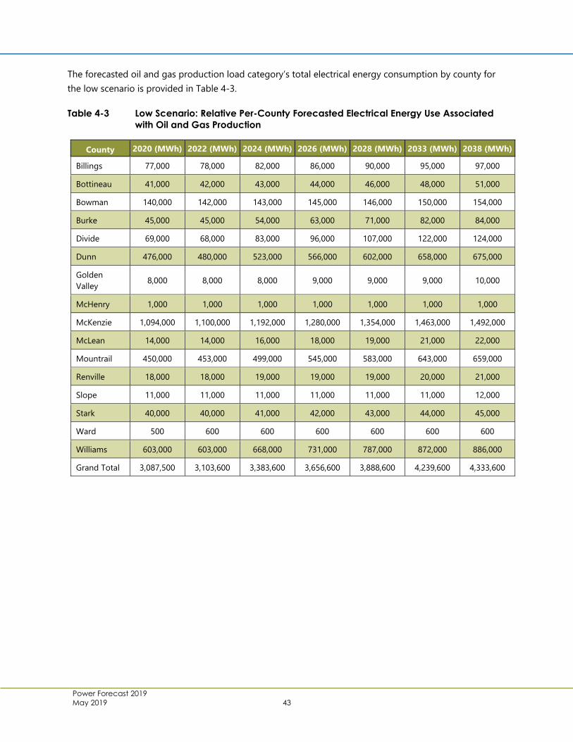
Power Forecast 2019

May 2019 43

The forecasted oil and gas production load category’s total electrical energy consumption by county for

the low scenario is provided in Table 4-3.

Table 4-3 Low Scenario: Relative Per-County Forecasted Electrical Energy Use Associated

with Oil and Gas Production

County 2020 (MWh) 2022 (MWh) 2024 (MWh) 2026 (MWh) 2028 (MWh) 2033 (MWh) 2038 (MWh)

Billings 77,000 78,000 82,000 86,000 90,000 95,000 97,000

Bottineau 41,000 42,000 43,000 44,000 46,000 48,000 51,000

Bowman 140,000 142,000 143,000 145,000 146,000 150,000 154,000

Burke 45,000 45,000 54,000 63,000 71,000 82,000 84,000

Divide 69,000 68,000 83,000 96,000 107,000 122,000 124,000

Dunn 476,000 480,000 523,000 566,000 602,000 658,000 675,000

Golden

Valley 8,000 8,000 8,000 9,000 9,000 9,000 10,000

McHenry 1,000 1,000 1,000 1,000 1,000 1,000 1,000

McKenzie 1,094,000 1,100,000 1,192,000 1,280,000 1,354,000 1,463,000 1,492,000

McLean 14,000 14,000 16,000 18,000 19,000 21,000 22,000

Mountrail 450,000 453,000 499,000 545,000 583,000 643,000 659,000

Renville 18,000 18,000 19,000 19,000 19,000 20,000 21,000

Slope 11,000 11,000 11,000 11,000 11,000 11,000 12,000

Stark 40,000 40,000 41,000 42,000 43,000 44,000 45,000

Ward 500 600 600 600 600 600 600

Williams 603,000 603,000 668,000 731,000 787,000 872,000 886,000

Grand Total 3,087,500 3,103,600 3,383,600 3,656,600 3,888,600 4,239,600 4,333,600

Power Forecast 2019

May 2019 44

The forecasted oil and gas production load category’s total electrical energy consumption by county for

the consensus scenario is provided in Table 4-4.

Table 4-4 Consensus Scenario: Relative Per-County Forecasted Electrical Energy Use

Associated with Oil and Gas Production


Billings 84,000 89,000 95,000 100,000 104,000 110,000 111,000

Bottineau 41,000 42,000 43,000 44,000 46,000 48,000 51,000

Bowman 140,000 142,000 143,000 145,000 146,000 150,000 154,000

Burke 62,000 73,000 87,000 99,000 109,000 122,000 123,000

Divide 96,000 110,000 132,000 150,000 164,000 180,000 181,000

Dunn 547,000 595,000 659,000 715,000 759,000 820,000 833,000

Golden Valley 8,000 9,000 9,000 9,000 10,000 10,000 10,000

McHenry 1,000 1,000 1,000 1,000 1,000 1,000 1,000

McKenzie 1,251,000 1,347,000 1,484,000 1,596,000 1,686,000 1,805,000 1,821,000

McLean 17,000 19,000 22,000 24,000 26,000 28,000 29,000

Mountrail 529,000 579,000 648,000 707,000 755,000 821,000 832,000

Renville 18,000 18,000 19,000 19,000 19,000 20,000 21,000

Slope 11,000 11,000 11,000 11,000 11,000 11,000 12,000

Stark 41,000 41,000 43,000 44,000 45,000 46,000 47,000

Ward 500 600 600 600 600 600 600

Williams 720,000 787,000 886,000 967,000 1,035,000 1,127,000 1,128,000

Grand Total 3,566,500 3,863,600 4,282,600 4,631,600 4,916,600 5,299,600 5,354,600

4.1.2 Large Industrial and Commercial

The forecasted large industrial and commercial load category’s total electrical energy consumption is

shown in Figure 4-5. Because the energy consumption within the large industrial and commercial load

category is comprised primarily of natural gas processing plants, the total forecasted electrical energy

consumption for electrical energy follows a similar trajectory as the projected gas production values

(Figure 2-3).

Power Forecast 2019

May 2019 45

(natural gas processing plants, refineries, and oil transmission pump stations)

Figure 4-5 Large Industrial and Commercial Sources Forecasted Electrical Energy

Consumption

The forecast estimates that an additional 2,735 GWh (low scenario) to 3,771 GWh (consensus) will be

consumed by natural gas processing plants, refineries, and oil transmission pipeline pump stations by the

end of the study period. Total consumption for this load category at the end of the study period is

estimated to more than double (or approximately a 200% increase for the low scenario and an

approximately 250% increase for the consensus scenario).

The forecasted results are reported by county in Table 4-5 and Table 4-6, however the locations of future

consumption for this category will be dependent upon where new infrastructure is constructed as

described in Section 2.2.2. Locations of potential future natural gas processing plants and refineries

assumed within the study are shown in Large Figure 2; as described in Section 2.2.2, one potential future

oil transmission pipeline was assumed within Williams, McKenzie, Dunn, Stark, Hettinger, and Adam

Counties.

Power Forecast 2019

May 2019 46


with Large Industrial and Commercial Sources


Adams - - - - 40 40 40

Billings 25,000 93,000 96,000 89,000 92,000 95,000 96,000

Bowman 37,000 39,000 44,000 78,000 85,000 96,000 101,000

Burke 7,000 6,000 7,000 6,000 7,000 6,000 7,000

Divide 34,000 103,000 121,000 147,000 166,000 195,000 209,000

Dunn 123,000 143,000 154,000 167,000 179,000 197,000 206,000

Golden Valley 20 20 20 20 20 20 20

Hettinger - - - - 70 70 70

McHenry 60 60 60 60 60 60 60

McKenzie 1,721,000 1,765,000 1,901,000 2,070,000 2,207,000 2,433,000 2,541,000

Mercer 20 20 20 20 20 20 20

Mountrail 335,000 298,000 284,000 291,000 292,000 299,000 307,000

Slope 7,000 7,000 8,000 6,000 7,000 8,000 8,000

Stark 60,000 116,000 120,000 111,000 114,000 118,000 120,000

Ward 100 100 100 100 100 100 100

Williams 765,000 874,000 1,055,000 1,208,000 1,337,000 1,565,000 1,670,000

Grand Total 3,114,200 3,444,200 3,790,200 4,173,200 4,486,310 5,012,310 5,265,310

Notes: Natural gas processing plants, refineries, and oil transmission pump stations only.

Where total MWh's by county decrease from one reported year to another, this is due to the method used to estimate

the locations of potential future natural gas processing plants. In some cases when a new or expanded gas plant is

introduced into the calculations, the result is that capacity from another geographic area is decreased, thereby lowering

the total estimated electrical energy consumption in a neighboring county.

Power Forecast 2019

May 2019 47


Associated with Large Industrial and Commercial Sources


Adams - - - - 40 40 40

Billings 27,000 94,000 98,000 98,000 97,000 96,000 98,000

Bowman 40,000 61,000 71,000 93,000 112,000 134,000 141,000

Burke 7,000 6,000 6,000 7,000 6,000 7,000 7,000

Divide 34,000 138,000 170,000 201,000 226,000 258,000 273,000

Dunn 128,000 163,000 181,000 198,000 195,000 199,000 207,000

Golden Valley 20 20 20 20 20 20 20

Hettinger - - - - 70 70 70

McHenry 60 60 60 60 60 60 60

McKenzie 1,791,000 2,013,000 2,235,000 2,452,000 2,635,000 2,914,000 3,033,000

Mercer 20 20 20 20 20 20 20

Mountrail 335,000 314,000 285,000 293,000 293,000 308,000 302,000

Slope 7,000 8,000 9,000 9,000 8,000 8,000 9,000

Stark 62,000 117,000 122,000 122,000 120,000 120,000 122,000

Ward 100 100 100 100 100 100 100

Williams 765,000 1,092,000 1,369,000 1,565,000 1,723,000 1,979,000 2,108,000

Grand Total 3,196,200 4,006,200 4,546,200 5,038,200 5,415,310 6,023,310 6,300,310

Notes: Natural gas processing plants, refineries, and oil transmission pump stations only.

Where total MWh’s by county decrease from one reported year to another, this is due to the method used to estimate

the locations of potential future natural gas processing plants. In some cases when a new or expanded gas plant is

introduced into the calculations, the result is that capacity from another geographic area is decreased, thereby lowering

the total estimated electrical energy consumption in a neighboring county.

4.1.3 Population

The forecasted population load category’s total electrical energy consumption is shown in Figure 4-6.

The relative per-county energy use associated with population grows steadily throughout the study

period for both the low scenario and the consensus scenario. Population growth rates within the NDSU

study included relatively continuous rates of growth and therefore the population load category followed.

Power Forecast 2019

May 2019 48

Figure 4-6 Population Forecasted Electrical Energy Consumption

Power Forecast 2019

May 2019 49

The forecasted population load category’s total electrical energy consumption by county for the low

scenario is provided in Table 4-7.


with Population


Adams 44,000 45,000 45,000 45,000 45,000 45,000 46,000

Billings 69,000 70,000 70,000 70,000 70,000 69,000 70,000

Bottineau 99,000 100,000 101,000 101,000 101,000 102,000 104,000

Bowman 21,000 21,000 22,000 22,000 22,000 22,000 22,000

Burke 54,000 55,000 55,000 56,000 55,000 55,000 55,000

Divide 26,000 25,000 25,000 25,000 25,000 25,000 25,000

Dunn 588,000 590,000 594,000 595,000 595,000 599,000 616,000

Golden Valley 151,000 154,000 157,000 159,000 160,000 161,000 161,000

Hettinger 128,000 129,000 129,000 129,000 129,000 127,000 129,000

McHenry 235,000 240,000 239,000 240,000 240,000 241,000 241,000

McKenzie 365,000 373,000 384,000 394,000 405,000 419,000 435,000

McLean 120,000 120,000 120,000 120,000 120,000 120,000 121,000

Mercer 165,000 165,000 165,000 165,000 164,000 163,000 163,000

Mountrail 1,032,000 1,056,000 1,108,000 1,141,000 1,175,000 1,215,000 1,259,000

Oliver 109,000 109,000 109,000 109,000 109,000 109,000 109,000

Pierce 38,000 38,000 38,000 38,000 38,000 38,000 38,000

Renville 85,000 85,000 85,000 85,000 85,000 85,000 86,000

Rolette 50,000 50,000 50,000 50,000 50,000 50,000 50,000

Sheridan 84,000 84,000 84,000 84,000 84,000 84,000 84,000

Slope 101,000 101,000 102,000 101,000 101,000 100,000 99,000

Stark 360,000 368,000 374,000 376,000 376,000 375,000 389,000

Ward 280,000 286,000 288,000 290,000 292,000 298,000 306,000

Wells 37,000 37,000 37,000 37,000 37,000 37,000 37,000

Williams 856,000 874,000 872,000 869,000 879,000 892,000 929,000

Grand Total 5,097,000 5,175,000 5,253,000 5,301,000 5,357,000 5,431,000 5,574,000

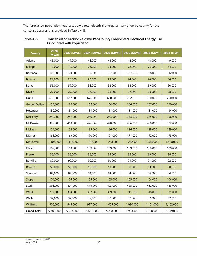
Power Forecast 2019

May 2019 50

The forecasted population load category’s total electrical energy consumption by county for the

consensus scenario is provided in Table 4-8.


Associated with Population

County 2020

(MWh) 2022 (MWh) 2024 (MWh) 2026 (MWh) 2028 (MWh) 2033 (MWh) 2038 (MWh)

Adams 45,000 47,000 48,000 48,000 48,000 48,000 49,000

Billings 72,000 72,000 73,000 73,000 72,000 73,000 74,000

Bottineau 102,000 104,000 106,000 107,000 107,000 108,000 112,000

Bowman 22,000 23,000 23,000 23,000 24,000 24,000 24,000

Burke 56,000 57,000 58,000 58,000 58,000 59,000 60,000

Divide 27,000 27,000 26,000 26,000 27,000 28,000 28,000

Dunn 639,000 657,000 676,000 690,000 702,000 720,000 750,000

Golden Valley 154,000 160,000 162,000 164,000 166,000 167,000 170,000

Hettinger 130,000 131,000 131,000 131,000 131,000 131,000 134,000

McHenry 240,000 247,000 250,000 253,000 253,000 255,000 256,000

McKenzie 392,000 409,000 426,000 440,000 456,000 488,000 522,000

McLean 124,000 124,000 125,000 126,000 126,000 128,000 129,000

Mercer 168,000 169,000 170,000 171,000 171,000 172,000 173,000

Mountrail 1,104,000 1,136,000 1,196,000 1,238,000 1,282,000 1,343,000 1,408,000

Oliver 109,000 109,000 109,000 109,000 109,000 109,000 109,000

Pierce 38,000 38,000 38,000 38,000 38,000 38,000 38,000

Renville 89,000 90,000 90,000 90,000 91,000 91,000 92,000

Rolette 50,000 50,000 50,000 50,000 50,000 50,000 50,000

Sheridan 84,000 84,000 84,000 84,000 84,000 84,000 84,000

Slope 104,000 105,000 105,000 105,000 105,000 104,000 104,000

Stark 391,000 407,000 419,000 423,000 425,000 432,000 453,000

Ward 297,000 304,000 307,000 309,000 311,000 318,000 331,000

Wells 37,000 37,000 37,000 37,000 37,000 37,000 37,000

Williams 906,000 946,000 977,000 1,005,000 1,030,000 1,101,000 1,162,000

Grand Total 5,380,000 5,533,000 5,686,000 5,798,000 5,903,000 6,108,000 6,349,000

Power Forecast 2019

May 2019 51

5 References

[1] North Dakota Transmission Authority, Annual Report (July 1, 2015 - June 30, 2016), 2016.

[2] Kadrmas, Lee & Jackson, Inc., Power Forecast 2012: Williston Basin Oil and Gas Related Electrical Load

Growth Forecast, 2012.

[3] State Historical Society of North Dakota, "Section 2: The Williston Basin," 2019. [Online]. Available:

https://www.ndstudies.gov/gr8/content/unit-i-paleocene-1200-ad/lesson-1-changing-

landscapes/topic-2-geology/section-2-williston-basin. [Accessed 4 March 2019].

[4] Energy & Environmental Research Center, "Geology," [Online]. Available:

http://www.undeerc.org/Bakken/geology.aspx. [Accessed 4 March 2019].

[5] J. A. LeFever and S. H. Nordeng, "Three Forks Formation," North Dakota Department of DMR Mineral

Resources Newsletter, vol. 35, no. 2, pp. 4-5, June 2008.

[6] S. A. Sonnenberg, Sequence Stratigraphy of the Bakken and Three Forks Formations, Williston Basin,

USA, 2017.

[7] T. O. Nesheim, Examination of Middle Three Forks (2nd Bench) Hydrocarbon Charge and Production,

vol. 45, 2018.

[8] North Dakota Pipeline Authority, "March 2019 NDPA Raw Forecast Data," 15 March 2019. [Online].

Available: Emailed to Barr from Justin Kringstad.

[9] North Dakota Geological Survey, Geologic Investigations No. 59: Bakken Formation Map Series: Sheet

1-3, 5, 2008.

[10] U.S. Energy Information Administration, "Appendix 2.C: Decline Curve Analysis," in Oil and Gas

Supply Module of the National Energy Modeling System: Model Documentation 2018, 2018.

[11] North Dakota State University, Williston Basin 2016: Employment, Population, and Housing Forecasts,

2017.

[12] Vision West ND, "Research & Reports," [Online]. Available: https://www.visionwestnd.com/research-

resources/?category=Webinar. [Accessed Aprl 2019].

[13] North Dakota, "Current Active Drilling Rig List," [Online]. Available:

https://www.dmr.nd.gov/oilgas/riglist.asp. [Accessed 24 April 2019].

Power Forecast 2019

May 2019 52

[14] Industrial Commission of North Dakota - North Dakota Pipeline Authority, The Pipeline Publication,

vol. V, 2012.

[15] B. Barnes, "North Dakota's gas flaring challenge lingers on," Petroleum Economist, 13 November

2018.

[16] U.S. Energy Information Administration, Natural Gas Weekly Update, 2017.

[17] A. Dalrymple, "North Dakota natural gas flaring hits record high; improvement expected in 2019,"

Bismarck Tribune, 25 December 2018.

[18] Industrial Commission of North Dakota Pipeline Authority, "Pipeline Industry Update," The Pipeline

Publication, vol. 10, no. 1, January 2019.

[19] Great Plains Energy Corridor; Bismarck State College, "Spotlight on North Dakota Energy 2017

Annual Report," 2017. [Online].

[20] U.S. Energy Information Administration, Electric Power Monthly with Data for February 2019, 2019.

Appendices

Appendix A

Large Figures

!(

!(

!(

!(

!(

!(

!(

!(

!(!(

!(

!(

!(

!(

!(

!(

!(

!(

!(

!(

!(

!(

Ward

Dunn

McLean

McKenzie

Stark

Williams

Slope

McHenry

Divide

Mountrail

Burke

Wells

Pierce

Bottineau

Mercer

Billings

AdamsBowman

Rolette

Oliver

Hettinger

Sheridan

Renville

GoldenValley

Tioga

Mott

Beach

Minot

Mohall

Bowman

Amidon

Medora

Crosby

Towner

Center

Beulah

Stanley

Washburn

Bowbells

Dickinson

Hettinger

Williston

Bottineau

New England

Watford City

Killdeer

Barr Footer: ArcGIS 10.6, 2019-05-09 11:18 File: I:\Projects\34\53\1076\Maps\Reports\Large Figure 1 Baseline Energy Load Year 2018.mxd User: MRQ

BASELINE ELECTRICAL ENERGYCONSUMPTION: 2018

Power Forecast 2019 Report:Williston Basin Oil and Gas Related

Electrical Load Growth ForecastNorth Dakota Transmission Authority

LARGE FIGURE 1

Study Area

Baseline Energy Load Year 2018

Low

Medium

High

0 10 20 30

Miles

!;N

!(

!(

!(

!(

!(

!(

!(

!(

!(!(

!(

!(

!(

!(

!(

!(

!(

!(

!(

!(

!(

!(

!4!4

!4

!:

!4

!:

!4!4

!4

!4

!:

!4

!4

!4

!4!4

!4!4!4!4

!4!4

!4

!4

!4

!4

!4 !4

!4

!4

!4

!4

!4

!4

!4

!4

!4!4

!4

!4

Ward

Dunn

McLean

McKenzie

Stark

Williams

Slope

McHenry

Divide

Mountrail

Burke

Wells

Pierce

Bottineau

Mercer

Billings

AdamsBowman

Rolette

Oliver

Hettinger

Sheridan

Renville

GoldenValley

Arrow

Norse

Tioga

DeWitt

Badland

Lignite

Belfield

Marmarth

Hay Butte

Roosevelt

Wild Basin

Bear CreekGrasslands

County Line

Stateline I

Prairie RoseSpring Brook

Watford City

Little Knife

Stateline II

Robinson Lake

Ray - Whiting

Red Wing Creek

Lonesome Creek

Garden Creek IGarden Creek II

Badlands - Targa

Ray - XTO Neeson

Dickinson Refinery

Garden Creek III

Ray

Mott

Beach

Minot

Mohall

Bowman

Amidon

Medora

Crosby

Towner

Center

Beulah

Stanley

Washburn

Bowbells

Dickinson

Hettinger

Williston

Bottineau

New England

Watford City

Killdeer

Sources: Esri, DeLorme, USGS, NPS, Sources: Esri, USGS, NOAA

Barr Footer: ArcGIS 10.6, 2019-05-09 11:17 File: I:\Projects\34\53\1076\Maps\Reports\Large Figure 2 Existing and Proposed Large Industrial Commercial Users.mxd User: MRQ

LARGE INDUSTRIAL/COMMERCIALSOURCES ASSUMED WITHIN PF19

Power Forecast 2019 Report:Williston Basin Oil and Gas Related

Electrical Load Growth ForecastNorth Dakota Transmission Authority

LARGE FIGURE 2

0 10 20 30

Miles

!;NStudy Area

!: Existing Refinery!4 Existing Gas Plant!: Proposed Refinery

!4 Proposed or Hypothetical Gas PlantCrude Oil Pipelines

Note: Liberty Pipeline is a proposed pipeline ofapproximately 175 miles within our study area.The location of the proposed pipeline is unknown.

!(

!(

!(

!(

!(

!(

!(

!(

!(!(

!(

!(

!(

!(

!(

!(

!(

!(

!(

!(

!(

!(

Wells

Ward

Dunn

McLeanMcKenzie

Stark

Williams

Slope

McHenry

Divide

Mountrail

Burke

Pierce

Bottineau

MercerBillings

AdamsBowman

Rolette

Oliver

Hettinger

Sheridan

Renville

GoldenValley

Mott

Tioga

Beach

Minot

Mohall

Bowman

Amidon

Medora

Crosby

Towner

Center

Beulah

Stanley

Washburn

Bowbells

Killdeer

Dickinson

Hettinger

Williston

Bottineau

New England

Watford City

Barr

Foote

r: ArcG

IS 10

.6, 20

19-05

-06 13

:38 Fi

le: I:\P

rojec

ts\34

\53\10

76\M

aps\R

eport

s\Larg

e Figu

re 3 F

orecas

t Ene

rgy Lo

ad Ye

ar 20

22.m

xd Us

er: M

RQ

ESTIMATED ELECTRICALENERGY CONSUMPTION: 2022Power Forecast 2019 Report:

Williston Basin Oil andGas Related Electrical Load

Growth ForecastNorth Dakota Transmission

AuthorityLARGE FIGURE 3

0 20 40

Miles

!;N

!(

!(

!(

!(

!(

!(

!(

!(

!(!(

!(

!(

!(

!(

!(

!(

!(

!(

!(

!(

!(

!(

GoldenValley

Ward

Dunn

McLeanMcKenzie

Stark

Williams

Slope

McHenry

Divide

Mountrail

Wells

Burke

Pierce

Bottineau

Mercer

Billings

AdamsBowman

Rolette

Oliver

Hettinger

Sheridan

Renville

Mott

Tioga

Beach

Minot

Mohall

Bowman

Amidon

Medora

Crosby

Towner

Center

Beulah

Stanley

Washburn

Bowbells

Killdeer

Dickinson

Hettinger

Williston

Bottineau

New England

Watford City

Low Scenar io Consensus Scenar io

Low

Medium

High

Estimated Energy LoadYear 2022

Study Area

!(

!(

!(

!(

!(

!(

!(

!(

!(!(

!(

!(

!(

!(

!(

!(

!(

!(

!(

!(

!(

!(

Wells

Ward

Dunn

McLeanMcKenzie

Stark

Williams

Slope

McHenry

Divide

Mountrail

Burke

Pierce

Bottineau

MercerBillings

AdamsBowman

Rolette

Oliver

Hettinger

Sheridan

Renville

GoldenValley

Mott

Tioga

Beach

Minot

Mohall

Bowman

Amidon

Medora

Crosby

Towner

Center

Beulah

Stanley

Washburn

Bowbells

Killdeer

Dickinson

Hettinger

Williston

Bottineau

New England

Watford City

Barr

Foote

r: ArcG

IS 10

.6, 20

19-05

-06 13

:42 Fi

le: I:\P

rojec

ts\34

\53\10

76\M

aps\R

eport

s\Larg

e Figu

re 4 F

orecas

t Ene

rgy Lo

ad Ye

ar 20

28.m

xd Us

er: M

RQ





0 20 40

Miles

!;N

!(

!(

!(

!(

!(

!(

!(

!(

!(!(

!(

!(

!(

!(

!(

!(

!(

!(

!(

!(

!(

!(

GoldenValley

Ward

Dunn

McLeanMcKenzie

Stark

Williams

Slope

McHenry

Divide

Mountrail

Wells

Burke

Pierce

Bottineau

Mercer

Billings

AdamsBowman

Rolette

Oliver

Hettinger

Sheridan

Renville

Mott

Tioga

Beach

Minot

Mohall

Bowman

Amidon

Medora

Crosby

Towner

Center

Beulah

Stanley

Washburn

Bowbells

Killdeer

Dickinson

Hettinger

Williston

Bottineau

New England

Watford City


Low

Medium

High


Study Area

!(

!(

!(

!(

!(

!(

!(

!(

!(!(

!(

!(

!(

!(

!(

!(

!(

!(

!(

!(

!(

!(

Wells

Ward

Dunn

McLeanMcKenzie

Stark

Williams

Slope

McHenry

Divide

Mountrail

Burke

Pierce

Bottineau

MercerBillings

AdamsBowman

Rolette

Oliver

Hettinger

Sheridan

Renville

GoldenValley

Mott

Tioga

Beach

Minot

Mohall

Bowman

Amidon

Medora

Crosby

Towner

Center

Beulah

Stanley

Washburn

Bowbells

Killdeer

Dickinson

Hettinger

Williston

Bottineau

New England

Watford City

Barr

Foote

r: ArcG

IS 10

.6, 20

19-05

-06 13

:52 Fi

le: I:\P

rojec

ts\34

\53\10

76\M

aps\R

eport

s\Larg

e Figu

re 5 F

orecas

t Ene

rgy Lo

ad Ye

ar 20

38.m

xd Us

er: M

RQ





0 20 40

Miles

!;N

!(

!(

!(

!(

!(

!(

!(

!(

!(!(

!(

!(

!(

!(

!(

!(

!(

!(

!(

!(

!(

!(

GoldenValley

Ward

Dunn

McLeanMcKenzie

Stark

Williams

Slope

McHenry

Divide

Mountrail

Wells

Burke

Pierce

Bottineau

Mercer

Billings

AdamsBowman

Rolette

Oliver

Hettinger

Sheridan

Renville

Mott

Tioga

Beach

Minot

Mohall

Bowman

Amidon

Medora

Crosby

Towner

Center

Beulah

Stanley

Washburn

Bowbells

Killdeer

Dickinson

Hettinger

Williston

Bottineau

New England

Watford City


Low

Medium

High


Study Area

Appendix B

Formulae used in Calculations

Equations Used but not provided in Report

1) Pump Efficiency

The pump efficiency can change from a minimum value of about 0.3 for a smaller sized ESP to a maximum of about 0.8 for a pump jack. But the average pump efficiency in a field for a specific age class of wells is a value dependent on the fraction of each type pump deployed. So for this work the pump efficiency as a function of age is approximated as:

n{age} = minimum [ 0.4 + .05*age, 0.8 ]

It can be seen that after age = 8 years the value of n will be a constant value of 0.8.

2) Pressure as Function of Age

pressure{age} = a0*e-(age/tp) + a1*age + a2*age2 + a3*age3

where age is the age of the well, and a0, a1, a2, a3 and t are coefficients specific to the geology of the well. In principle the coefficients could be different for each well. However, for a geographic region at a particular interval of history, the completion methods and geology are similar enough that a composite curve can be used.

3) Production Energy production_energy = ENERGY * (oil_production * 0.85 + water_production * 1.2)

the specific gravity of crude oil from the Bakken is about 0.85, and the produced water is 1.2

4) Age of Well Algorithm

An algorithm for computing the power is shown below.

For FIELD = aaa to zzz;

For YEAR = 2014 to 2040;

For AGE = 0 to 15; 'decide whether 15 years is good enough

Select {a0, a1, a2, a3, tp, new_production} From FIELD.(YEAR-AGE)];

new_water = new_production * w_o_r; 'decide whether to use a constant for water/oil ratio

energy_production = ENERGY{age}*(new_production*0.85+new_water *1.2);

cumulative_energy = cumulative_energy + energy_production;

Next AGE

Select {oil_production, water_production} From [FIELD.(YEAR-16)]

cumulative_energy = ENERGY{16}*(oil_production*0.85+water_production *1.2)*volume{16};

Next YEAR

5) Energy Information Administration (EIA) of the US Department of Energy (DOE) Decline Curve

New oil production is calculated using an algorithm described in pseudocode below:

:volume{age} = 1/(1+b*Di*age*12)^(1/b)

For FIELD = aaa To zzz;

For Year = 2020 To 2040;

For AGE = 1 to 20;

Select {b, Di, oil_production} From FIELD.(YEAR-AGE);

Declination = FIELD.(YEAR-AGE).new_production * (1-volume{age});

new_oil = new_oil + Declination;

Next AGE;

FIELD.YEAR.new_production = new_oil + FIELD.YEAR.oil_production-FIELD.(YEAR-1).oil_production;

Next YEAR;

Next FIELD;

This algorithm ignores declining production volumes of wells more than 20 years old. This is believed to not be significant because either a) the wells have by then declined to a small and irrelevant level; or b) they have been reworked and will be counted as new production.

6) Energy Consumed by the Gathering Pumps and Compressor Work

pump_work = oil_production*length *(1-trucked_oil)* 0.15 + water_production*length*(1-trucked_water)* 0.15 + water_production *SWD_pressure /55000

Where the units for production is in barrels/day and the gathering network segment length is in miles.

Gas gathering power consumption is also a function of volume production, length of gathering pipelines, and fraction of gas flared. The formula is:

compressor_work = gas_production * length *(1-flare_fraction) * 27

Where the units for production is in million standard cubic feet per day and the gathering network segment length is in miles.

NOTE: in this context “oilfield” means a geographic region in North Dakota which produces hydrocarbons; “FIELD” means a piece of data stored in a RECORD of a data base.

Appendix C

PF19 Sensitivities Analysis Memorandum

Barr Engineering Co. 234 West Century Avenue, Bismarck, ND 58503 701.255.5460 www.barr.com

Memorandum

To: File

From: Sarah Johnson and Don Kopecky

Subject: PF19 Sensitivities Analysis

Date: May 8, 2019

1.0 Introduction

The purpose of this memo is to summarize what we think are the most impactful sensitivities surrounding

methodologies used within the PF19. As described in the PF19, a number of formulae and information

sources were used to compile the electrical energy consumption forecast. Sensitivities surrounding how

those forecasts were completed with the greatest potential for impact include:

production-based forecasting and continuation of existing technologies/similar production areas

(Section 2.0),

population forecast growth rate application (Section 3.0),

length of gathering lines (Section 4.0), and

initial well pressure (Section 5.0).

This memo does not address or confirm sensitivities included within NDPA’s oil and gas production

estimates or NDSU’s population forecast estimates, as those were not validated by Barr and instead used

as the best publicly available datasets.

We recognize unknown factors may also impact the results of the study. Therefore, the PF19 was designed

so it may be readily updated to account for changes.

2.0 Production-Based Forecasting and Continuation of Existing Technologies/Similar

Production Areas

The PF19’s approach was to estimate future electric energy consumption growth as a function of

projected oil and gas production volumes available from NDPA. The PF12 also forecasted future electrical

energy consumption growth as a result of increased oil and gas production but instead forecasted it as a

function of specific well counts and rig counts (which are incorporated into the PF19 as a function of the

NDPA and NDSU forecasts which use many of those same factors as the PF12 for their forecasts).

In both cases, the forecasts are limited by the unknown which includes future oil prices, regulations, North

Dakota policy, and potentially most important – future technological advances that would increase

efficiency and enhance oil recovery at wells as well at the geographic extents of where new development

will occur. Because the PF19 assumes that current practices are expected to largely carry forward into the

To: File



Date: May 8, 2019

Page: 2

\\barr.com\projects\Bismarck\34 ND\53\34531076 NDIC Transmission Study\WorkFiles\Report\Appendices\C Sens Analysis\Sensitivities Memo v1d6.docx

future, the calculations used to estimate future production of oil and gas are not altered throughout the

study period for new technologies, but are modified to reflect decline curves. The PF19 also assumes that

most of the new production of oil and gas will occur where the currently highest producing areas are

located. As described in the FP19, production is extended outward from this focal area however the

distribution outward is projected out very gradually.

To better understand the potential sensitivities around forecasting as a means of well and rig counts

(PF12) versus forecasted volumes (PF19), Barr compared the rate of growth for reported years between

the two studies. Generally speaking, the FP12 estimate continue “boom” like growth for the first half of

the study period, and the PF19’s year-to-year growth rates appear to be steadier than the PF12. It is

unknown however, whether the changes in the rates of growth are attributable to the different methods

used to forecast (as a function of volumes versus a function of counts), different assumptions used for

future oil and gas productions, or is attributable to more efficient means of extraction and production.

Table 2-1 compares the PF12’s first and second halves’ growth rates of their respective study periods, as

well as compares the overall growth rate from the beginning to the end of the respective 20-year study

periods.

Table 2-1 Comparing PF12 to PF19 Growth Rates

Study and Point

of Comparison

First Half of Study Period Second Half of Study

Period

Full Study Period

PF12: total

demand (MW) 1

From 2012 – 2022, the

PF12 forecasted in increase

of 247% in total MW.

From 2023 – 2032, the

PF12 forecasted an

increase of 126% in total

KWh.

Overall, the PF12 forecasted an

increase of 312% from the

study period’s beginning to

end.

PF12: total KWh 2 From 2012 – 2022, the

PF12 forecasted in increase

of 278% in total KWh.

From 2023 – 2032, the

PF12 forecasted an


KWh.




end.

PF19 Low

Scenario: total

KWh

From 2018 – 2028, the

PF19 forecasted an


KWh.

From 2029 – 2038, the

PF19 forecasted an


KWh.




end.

PF19 Consensus

Scenario: total

KWh

From 2018 – 2028, the

PF19 forecasted an


KWh.

From 2029 – 2038, the

PF19 forecasted an


KWh.




end. 1 Per numbers provided in Table 1 of the PF12 Summary 2 Per numbers provided in Table 3 of the PF12.

The PF12’s study area was more inclusive than the PF19’s and extended into the states of South Dakota,

Montana, and Wyoming. The PF12 results were organized by regions whereas the PF19 results were

organized by county. Barr compared the 2027 and 2032 reporting years to identify potential sensitivities

around the geographic extents of forecasted growth. The PF12’s reported numbers for this year had high

agreement (i.e., where the PF12’s forecasted numbers were within 10% of the PF19’s forecasted numbers)

To: File



Date: May 8, 2019

Page: 3


in the higher oil and gas producing counties of Williams, Mountrail, and Dunn. The biggest difference

between the PF12 and PF19’s compared reporting year’s results is that the PF12 forecasted significantly

more growth across the PF12’s Region 1 counties further outside of the highest producing areas.

Specifically, the PF12 estimated more growth in Divide, Burke, Ward, McLean, Bottineau, and Rollete

Counties. The PF12 seemed more optimistic in future production growth in these areas; and the PF19

forecasts less geographic expansion of future production.

The PF19’s greatest sensitivity around its methodology would be a change in the gas forecast (similar to

the PF12), but it would also be sensitive to significant changes in extraction and processing

methodologies and a potential geographic difference in what was assumed for future areas of oil and gas

production.

3.0 Population Broad Load Category Growth-Rate Forecasting Method

Approximately half of the baseline electrical energy consumption in the PF19 was allocated to the

population broad load category. Specifically, approximately 3,000 GWh were allocated to oil and gas,

approximately 2,500 GWh were allocated to large industrial/commercial, and approximately 5,000 GWh

were allocated to population. This load category was forecasted as a function of NDSU’s population

forecast growth rates.

Because commercial users not directly related to oil and gas production (i.e., commercial and industrial

users that are not natural gas processing plants, oil transmission pump stations, or terminals) are included

within the population base load category, these commercial and industrial users are subject to the

estimated population forecast rate growths established in the NDSU study. The overall growth rates from

the beginning of the study period to the end of the study period in the population category are provided

in Table 3-1 and more specific information regarding annual growth rates are provided in Appendix B of

the PF19.

Table 3-1 Population Base Load Category Growth Rates by County

County 2018 - 2038

Population Growth 1

2018 - 2038

O&G Growth 1

Adam 11% 0%

Billings 7% 47%

Bottineau 11% 26%

Bowman 15% 0%

Burke 10% 193%

Divide 5% 175%

Dunn 22% 81%

Golden Valley 15% 31%

Hettinger 6% 0%

McHenry 10% 31%

McKenzie 41% 71%

To: File



Date: May 8, 2019

Page: 4


County 2018 - 2038

Population Growth 1

2018 - 2038

O&G Growth 1

McLean 5% 126%

Mercer 3% 0%

Mountrail 33% 92%

Oliver 6% 0%

Pierce 2% 0%

Renville 25% 12%

Rolette 15% 0%

Sheridan 34% 0%

Slope 11% 0%

Stark 7% 21%

Ward 11% 3%

Wells 15% 0%

Williams 10% 94%

1 Reported rates pertain to the consensus scenario of the NDSU

population study.

4.0 Gathering Line Length

The pumping work necessary to gather the liquid and gas and transport it to their respective destinations

is directly related to the length and diameter of pipes in the gathering network. These values are

impossible to define precisely across the entire study area, and will change over time. Consequently the

PF19 estimates are based on reasonable values for fluid velocity, pressure drop, and locations of well

fields and processing facilities. Variation in specific gathering energy of oil or water for a range of

conditions is given in the Table 4-1.

Table 4-1 Variation in Specific Gathering Energy of Oil or Water

Condition Pipeline length

(miles)

Pressure drop

(psid/mile)

Pumping work

kwh/bbl

MODEL BASIS 12 170 1.8

Long pipeline and high pressure 20 250 4.4

Short pipeline and low pressure 5 80 .35

The pumping work in the table spans an order of magnitude, which implies that there could be a

considerable error introduced by using the wrong values. This underscores the importance of calibrating

the model to the 2018 baseline data. Using actual data for a representative cooperative the computed

gathering energy agreed within about 7% of reported energy sales. Consequently, the parameters used in

the model basis are most likely within 10% of the actual field average values. Gathering line energy use at

the baseline is approximately 1,314 GWh or 12 % of the total energy consumption.

To: File



Date: May 8, 2019

Page: 5


5.0 Initial Well Pressure

Initial well pressure is known to vary throughout the basin. Tim Nesheim (ND Geologic Survey) provided

the following information to Barr about pressure in the Bakken Formation:

Typically, most reservoirs in North Dakota are at a normal pressure gradient during initial production,

which is around ~0.46 psi/ft. However, the fluid system in the Bakken Formation is overpressured due to

a combination of very low rock permeability and the large amount of oil pressure. So without going into

too much detail, the initial reservoir pressure of the Bakken is going to be a combination of depth and

fluid pressure gradient. Below is a fluid pressure map for the Bakken presented at a meeting in 2013 by

a Colorado School of Mines student.

Based on the map below, the highest fluid pressure gradients for the Bakken Formation are in and

around northwestern Dunn County, which includes the Lost Bridge Field. In the Lost Bridge Field, the

Bakken Formation is at a TVD (true vertical depth) of around ~10,600 ft., and with a fluid pressure

gradient of ~0.76 psi/ft, the Bakken fluid pressure would be a little over 8,000 psi. Conversely, in

northern Divide County in the Colgan Field, the Bakken is probably close to normal pressure (~0.46

psi/ft.) at a depth of ~8,000 ft. and probably has/had an initial reservoir pressure of ~3,700 psi. So your

rule of thumb ~5,500 psi initial reservoir pressure is a middle of the road value, and the 3,000 psi is an

underestimate.

To: File



Date: May 8, 2019

Page: 6


The highest overpressures in the Middle Bakken are correlated to peak hydrocarbon generation

(after Theloy and Sonnenberg, 2013). 1

Figure 5-1 Middle Bakken Pressure Gradient

Our calculation uses 5500 psig initial reservoir pressure for all fields, rather than following the pressure

distribution shown in the map. We then calculate actual reservoir pressure at the time of production using

the same decline curve as developed by EIA for production volume.

To get an idea of how the below ground energy will be affected by reservoir initial pressure we evaluated

a few bounding cases. The pump work A was calculated first using an initial pressure of 5500, and the

pressure decline was based on a mid-year convention. The pump work B was then compared using an

initial pressure based on the pressure gradient and a monthly pressure decline. Using the parameters for

Lost Bridge Field, the specific power computed using the two different pressures is shown below.

1 Source: Email dated April 17, 2019 from Tim Nesheim (UND) to Justin Kringstad (NDPA).

To: File



Date: May 8, 2019

Page: 7


Year 0 1 2 3 4

work A = 10.55 13.05 13.17 13.18 13.18

work B = 7.05 12.89 13.16 13.18 13.18

Repeating this procedure for the Colgan Field gives:

Year 0 1 2 3 4

work A= 11.58 13.14 13.18 13.18 13.18

work B = 10.39 13.13 13.18 13.18 13.18

Therefore, using an initial pressure of 5500 psig across the entire basin with a mid-year decline

calculation, tends to overestimate the pump work required as compared to using field specific pressure

gradients and a monthly decline calculation. This difference is a maximum of 33% higher in Lost Bridge

Field at Year 0 but quickly declines to insignificance by Year 2. For Colgan Field the difference at Year 0 is

only about 10%. The below ground energy use affected by this estimate accounted for approximately

112 GWh in the baseline or 1 % of the total energy consumption.

Appendix D

NDSU Population Forecasts

Historical and Projected Service Populations, by Economic Scenario, Adams County, North Dakota 2002 ‐ 2040

Low Scenarios Moderate Scenarios High Scenarios

Year Estimated Low1 Mid High2 Low2 Mid High2 Low2 Mid High1

2002 2,683

2003 2,666

2004 2,619

2005 2,572

2006 2,540

2007 2,534

2008 2,543

2009 2,504

2010 2,508

2011 2,469

2012 2,458

2013 2,582

2014 2,582

2015 2,555

2016 2,516 2,516 2,516 2,502 2,502 2,502 2,502 2,502 2,502

2017 2,500 2,504 2,508 2,536 2,540 2,540 2,570 2,570 2,570

2018 2,535 2,541 2,546 2,599 2,615 2,619 2,658 2,661 2,669

2019 2,561 2,569 2,578 2,630 2,648 2,663 2,707 2,728 2,738

2020 2,593 2,604 2,617 2,667 2,688 2,714 2,763 2,803 2,815

2021 2,632 2,645 2,662 2,737 2,762 2,783 2,837 2,861 2,884

2022 2,627 2,642 2,661 2,747 2,774 2,797 2,875 2,901 2,926

2023 2,647 2,663 2,685 2,772 2,801 2,827 2,875 2,904 2,931

2024 2,650 2,668 2,693 2,798 2,829 2,857 2,892 2,923 2,952

2025 2,650 2,670 2,697 2,806 2,838 2,869 2,907 2,940 2,971

2026 2,640 2,660 2,689 2,802 2,835 2,868 2,912 2,947 2,980

2027 2,632 2,652 2,682 2,800 2,835 2,869 2,917 2,955 2,989

2028 2,624 2,646 2,677 2,799 2,836 2,872 2,924 2,964 3,000

2029 2,647 2,668 2,699 2,805 2,842 2,880 2,929 2,970 3,008

2030 2,646 2,668 2,698 2,802 2,841 2,879 2,933 2,976 3,015

2031 2,669 2,691 2,721 2,799 2,839 2,878 2,937 2,982 3,022

2032 2,664 2,687 2,718 2,800 2,841 2,883 2,945 2,992 3,034

2033 2,663 2,687 2,721 2,805 2,848 2,892 2,957 3,006 3,051

2034 2,662 2,687 2,723 2,809 2,855 2,901 2,969 3,020 3,067

2035 2,663 2,690 2,730 2,817 2,865 2,914 2,984 3,038 3,087

2036 2,660 2,689 2,733 2,822 2,872 2,923 2,996 3,051 3,102

2037 2,659 2,689 2,737 2,828 2,880 2,934 3,010 3,066 3,120

2038 2,660 2,693 2,743 2,836 2,890 2,946 3,025 3,083 3,139

2039 2,663 2,698 2,752 2,846 2,903 2,961 3,043 3,103 3,160

2040 2,671 2,707 2,765 2,860 2,919 2,980 3,065 3,126 3,186

1Developed from extrapolation of main forecasts. 2Developed from interpolation between main forecasts.

Historical and Projected Service Populations, by Economic Scenario, Billings County, North Dakota 2002 ‐ 2040


Year Actual Low1 Mid High2 Low2 Mid High2 Low2 Mid High1

2002 933

2003 921

2004 929

2005 869

2006 851

2007 831

2008 827

2009 824

2010 847

2011 921

2012 1,038

2013 1,047

2014 1,069

2015 1,051

2016 1,018 1,018 1,018 1,018 1,018 1,018 1,018 1,018 1,018

2017 1,015 1,016 1,017 1,021 1,027 1,032 1,037 1,040 1,045

2018 1,011 1,014 1,016 1,027 1,036 1,046 1,054 1,061 1,071

2019 1,015 1,019 1,024 1,045 1,055 1,070 1,085 1,095 1,108

2020 1,028 1,030 1,037 1,061 1,073 1,085 1,098 1,113 1,127

2021 1,036 1,040 1,049 1,069 1,083 1,094 1,109 1,124 1,138

2022 1,041 1,048 1,057 1,073 1,084 1,098 1,110 1,128 1,146

2023 1,040 1,051 1,062 1,075 1,087 1,101 1,114 1,132 1,150

2024 1,044 1,053 1,064 1,078 1,090 1,105 1,117 1,138 1,159

2025 1,045 1,055 1,065 1,078 1,090 1,106 1,120 1,141 1,163

2026 1,043 1,053 1,065 1,080 1,089 1,104 1,122 1,145 1,169

2027 1,036 1,047 1,062 1,079 1,085 1,101 1,122 1,146 1,171

2028 1,031 1,042 1,058 1,077 1,084 1,099 1,123 1,149 1,175

2029 1,026 1,037 1,055 1,075 1,082 1,098 1,124 1,151 1,177

2030 1,022 1,033 1,049 1,072 1,081 1,096 1,124 1,151 1,179

2031 1,017 1,031 1,047 1,070 1,080 1,097 1,122 1,151 1,179

2032 1,015 1,032 1,047 1,067 1,081 1,098 1,124 1,153 1,183

2033 1,015 1,032 1,050 1,067 1,085 1,102 1,127 1,158 1,189

2034 1,015 1,033 1,053 1,070 1,090 1,108 1,131 1,163 1,196

2035 1,015 1,035 1,058 1,077 1,097 1,109 1,137 1,171 1,205

2036 1,015 1,036 1,061 1,079 1,100 1,115 1,141 1,176 1,211

2037 1,014 1,038 1,063 1,082 1,103 1,118 1,146 1,183 1,219

2038 1,014 1,042 1,067 1,089 1,108 1,123 1,153 1,190 1,228

2039 1,015 1,044 1,073 1,094 1,114 1,131 1,160 1,199 1,238

2040 1,017 1,046 1,079 1,100 1,122 1,139 1,169 1,210 1,250


Historical and Projected Service Populations, by Economic Scenario, Bottineau County, North Dakota 2002 ‐ 2040



2002 7,150

2003 6,990

2004 6,954

2005 6,813

2006 6,776

2007 6,712

2008 6,624

2009 6,579

2010 6,608

2011 6,743

2012 6,885

2013 7,013

2014 6,931

2015 6,922

2016 6,899 6,899 6,899 6,899 6,899 6,899 6,899 6,899 6,899

2017 6,831 6,837 6,841 6,921 6,961 6,989 7,052 7,052 7,052

2018 6,868 6,882 6,889 6,978 7,022 7,069 7,167 7,168 7,167

2019 6,892 6,912 6,932 7,050 7,102 7,176 7,296 7,308 7,322

2020 6,942 6,962 6,986 7,103 7,168 7,232 7,365 7,383 7,398

2021 6,984 6,993 7,014 7,172 7,240 7,308 7,462 7,481 7,500

2022 7,009 7,025 7,043 7,227 7,297 7,368 7,551 7,572 7,593

2023 7,030 7,047 7,067 7,270 7,344 7,417 7,628 7,651 7,674

2024 7,047 7,066 7,089 7,318 7,394 7,470 7,708 7,733 7,757

2025 7,060 7,080 7,105 7,348 7,427 7,505 7,768 7,799 7,833

2026 7,060 7,081 7,107 7,400 7,481 7,562 7,839 7,867 7,895

2027 7,058 7,080 7,106 7,407 7,490 7,574 7,860 7,890 7,919

2028 7,054 7,076 7,103 7,418 7,503 7,589 7,898 7,930 7,961

2029 7,042 7,064 7,091 7,417 7,504 7,591 7,912 7,945 7,978

2030 7,032 7,053 7,080 7,415 7,504 7,592 7,922 7,957 7,990

2031 7,044 7,066 7,092 7,416 7,505 7,604 7,921 7,957 7,992

2032 7,068 7,090 7,118 7,433 7,538 7,642 7,960 7,998 8,035

2033 7,089 7,113 7,143 7,464 7,570 7,677 8,006 8,046 8,084

2034 7,104 7,129 7,161 7,488 7,597 7,707 8,033 8,075 8,115

2035 7,126 7,152 7,187 7,516 7,630 7,743 8,075 8,118 8,161

2036 7,177 7,206 7,244 7,577 7,692 7,807 8,141 8,185 8,229

2037 7,227 7,258 7,298 7,642 7,759 7,876 8,218 8,264 8,309

2038 7,269 7,301 7,345 7,700 7,819 7,937 8,283 8,331 8,378

2039 7,308 7,342 7,389 7,752 7,873 7,994 8,346 8,395 8,444

2040 7,349 7,384 7,434 7,803 7,927 8,050 8,410 8,461 8,511


Historical and Projected Service Populations, by Economic Scenario, Bowman County, North Dakota 2002 ‐ 2040



2002 3,271

2003 3,235

2004 3,229

2005 3,249

2006 3,177

2007 3,198

2008 3,261

2009 3,272

2010 3,316

2011 3,363

2012 3,534

2013 3,588

2014 3,552

2015 3,553

2016 3,565 3,565 3,565 3,565 3,565 3,565 3,565 3,565 3,565

2017 3,327 3,332 3,334 3,497 3,508 3,530 3,628 3,649 3,672

2018 3,370 3,382 3,399 3,546 3,565 3,598 3,736 3,762 3,785

2019 3,447 3,464 3,481 3,642 3,662 3,686 3,844 3,874 3,894

2020 3,528 3,538 3,551 3,720 3,745 3,768 3,944 3,962 3,990

2021 3,569 3,581 3,596 3,801 3,825 3,850 4,033 4,058 4,082

2022 3,619 3,632 3,649 3,850 3,873 3,894 4,098 4,120 4,141

2023 3,644 3,659 3,679 3,883 3,908 3,931 4,142 4,166 4,190

2024 3,667 3,684 3,706 3,916 3,942 3,967 4,186 4,212 4,237

2025 3,687 3,705 3,730 3,945 3,974 4,000 4,226 4,254 4,282

2026 3,694 3,713 3,739 3,961 3,991 4,019 4,254 4,284 4,313

2027 3,701 3,721 3,748 3,977 4,009 4,039 4,281 4,313 4,344

2028 3,708 3,728 3,757 3,993 4,026 4,058 4,293 4,326 4,359

2029 3,712 3,732 3,760 4,004 4,038 4,070 4,296 4,330 4,364

2030 3,715 3,735 3,763 4,002 4,037 4,069 4,296 4,333 4,368

2031 3,722 3,743 3,771 4,000 4,036 4,070 4,309 4,352 4,379

2032 3,730 3,752 3,781 4,017 4,054 4,090 4,324 4,364 4,402

2033 3,742 3,765 3,796 4,037 4,076 4,115 4,356 4,397 4,438

2034 3,744 3,768 3,801 4,050 4,091 4,132 4,375 4,418 4,461

2035 3,743 3,768 3,805 4,059 4,102 4,145 4,394 4,438 4,483

2036 3,728 3,755 3,794 4,056 4,101 4,145 4,401 4,447 4,493

2037 3,713 3,742 3,785 4,052 4,099 4,145 4,408 4,456 4,503

2038 3,701 3,731 3,776 4,051 4,099 4,147 4,416 4,465 4,514

2039 3,688 3,720 3,768 4,048 4,098 4,149 4,423 4,474 4,525

2040 3,680 3,714 3,764 4,051 4,102 4,154 4,435 4,488 4,540 1Developed from extrapolation of main forecasts. 2Developed from interpolation between main forecasts.

Historical and Projected Service Populations, by Economic Scenario, Burke County, North Dakota 2002 ‐ 2040



2002 2,240

2003 2,208

2004 2,190

2005 2,129

2006 2,097

2007 2,025

2008 1,952

2009 1,932

2010 1,993

2011 2,093

2012 2,250

2013 2,362

2014 2,368

2015 2,350

2016 2,339 2,339 2,339 2,339 2,339 2,339 2,339 2,339 2,339

2017 2,269 2,276 2,280 2,316 2,319 2,322 2,349 2,348 2,349

2018 2,298 2,307 2,316 2,384 2,393 2,403 2,442 2,452 2,466

2019 2,330 2,342 2,355 2,426 2,441 2,452 2,506 2,517 2,533

2020 2,366 2,382 2,398 2,468 2,483 2,500 2,559 2,577 2,595

2021 2,390 2,408 2,426 2,497 2,514 2,533 2,598 2,617 2,639

2022 2,398 2,417 2,435 2,508 2,526 2,547 2,613 2,638 2,659

2023 2,404 2,425 2,447 2,519 2,539 2,560 2,628 2,652 2,677

2024 2,420 2,442 2,466 2,537 2,560 2,583 2,642 2,669 2,696

2025 2,425 2,448 2,472 2,544 2,570 2,596 2,658 2,684 2,715

2026 2,428 2,453 2,478 2,554 2,579 2,605 2,668 2,695 2,721

2027 2,428 2,453 2,479 2,554 2,578 2,608 2,668 2,697 2,724

2028 2,423 2,449 2,476 2,555 2,578 2,611 2,677 2,708 2,736

2029 2,422 2,448 2,474 2,559 2,579 2,617 2,687 2,719 2,749

2030 2,410 2,437 2,465 2,556 2,585 2,615 2,696 2,729 2,759

2031 2,402 2,427 2,454 2,553 2,582 2,614 2,696 2,735 2,769

2032 2,397 2,423 2,450 2,558 2,585 2,620 2,709 2,744 2,778

2033 2,402 2,429 2,458 2,567 2,597 2,630 2,724 2,761 2,796

2034 2,395 2,424 2,454 2,574 2,598 2,637 2,737 2,770 2,811

2035 2,395 2,425 2,457 2,575 2,605 2,646 2,743 2,783 2,821

2036 2,387 2,419 2,453 2,579 2,608 2,653 2,757 2,798 2,838

2037 2,383 2,417 2,453 2,586 2,618 2,663 2,772 2,814 2,855

2038 2,385 2,421 2,459 2,595 2,629 2,676 2,786 2,830 2,872

2039 2,392 2,429 2,469 2,606 2,643 2,690 2,799 2,843 2,887


Historical and Projected Service Populations, by Economic Scenario, Divide County, North Dakota 2002 ‐ 2040



2002 2,231

2003 2,245

2004 2,227

2005 2,199

2006 2,156

2007 2,139

2008 2,094

2009 2,052

2010 2,104

2011 2,199

2012 2,373

2013 2,463

2014 2,652

2015 2,638

2016 2,681 2,681 2,681 2,681 2,681 2,681 2,681 2,681 2,681

2017 2,648 2,652 2,657 2,698 2,707 2,715 2,763 2,780 2,794

2018 2,635 2,644 2,651 2,713 2,729 2,740 2,816 2,833 2,853

2019 2,619 2,629 2,639 2,733 2,746 2,760 2,839 2,866 2,886

2020 2,608 2,621 2,635 2,741 2,755 2,768 2,853 2,878 2,898

2021 2,587 2,603 2,618 2,728 2,743 2,758 2,853 2,879 2,899

2022 2,562 2,579 2,597 2,706 2,723 2,740 2,839 2,863 2,884

2023 2,535 2,554 2,573 2,688 2,706 2,724 2,820 2,842 2,861

2024 2,523 2,543 2,563 2,677 2,697 2,716 2,814 2,834 2,852

2025 2,510 2,531 2,553 2,670 2,691 2,712 2,805 2,827 2,846

2026 2,488 2,510 2,532 2,654 2,676 2,698 2,789 2,812 2,834

2027 2,484 2,506 2,530 2,658 2,681 2,704 2,794 2,819 2,841

2028 2,497 2,520 2,544 2,680 2,704 2,728 2,821 2,847 2,871

2029 2,509 2,531 2,555 2,702 2,727 2,751 2,846 2,873 2,898

2030 2,522 2,545 2,569 2,723 2,749 2,774 2,874 2,902 2,928

2031 2,528 2,551 2,574 2,739 2,765 2,791 2,895 2,924 2,952

2032 2,535 2,559 2,583 2,757 2,784 2,811 2,918 2,949 2,977

2033 2,549 2,574 2,599 2,778 2,807 2,835 2,947 2,979 3,009

2034 2,564 2,590 2,617 2,802 2,832 2,862 2,978 3,011 3,043

2035 2,576 2,605 2,633 2,816 2,848 2,880 3,007 3,035 3,068

2036 2,577 2,606 2,636 2,830 2,863 2,896 3,024 3,059 3,093

2037 2,571 2,601 2,633 2,831 2,865 2,899 3,034 3,071 3,106

2038 2,565 2,597 2,631 2,833 2,868 2,903 3,042 3,080 3,117

2039 2,565 2,598 2,633 2,839 2,875 2,912 3,056 3,095 3,133


Historical and Projected Service Populations, by Economic Scenario, Dunn County, North Dakota 2002 ‐ 2040


Year Estimated Low Mid High Low Mid High Low Mid High

2002 3,678

2003 3,657

2004 3,609

2005 3,538

2006 3,508

2007 3,512

2008 3,532

2009 3,549

2010 3,648

2011 4,023

2012 4,665

2013 4,887

2014 5,327

2015 5,214

2016 4,917 4,917 4,917 4,917 4,917 4,917 4,917 4,917 4,917

2017 4,913 4,958 5,004 5,053 5,087 5,121 5,152 5,196 5,212

2018 4,909 4,969 5,030 5,159 5,215 5,261 5,339 5,429 5,470

2019 4,905 4,980 5,055 5,270 5,342 5,412 5,501 5,632 5,728

2020 4,901 4,991 5,081 5,335 5,424 5,511 5,625 5,783 5,941

2021 4,894 4,999 5,104 5,397 5,503 5,608 5,794 5,970 6,146

2022 4,887 5,007 5,126 5,458 5,582 5,704 5,908 6,100 6,291

2023 4,897 5,022 5,148 5,520 5,660 5,800 6,030 6,236 6,441

2024 4,909 5,041 5,172 5,581 5,739 5,895 6,099 6,316 6,533

2025 4,922 5,061 5,199 5,642 5,817 5,991 6,173 6,403 6,632

2026 4,903 5,049 5,194 5,694 5,859 6,055 6,224 6,469 6,712

2027 4,898 5,051 5,204 5,714 5,916 6,103 6,288 6,546 6,803

2028 4,895 5,056 5,216 5,747 5,958 6,167 6,353 6,626 6,898

2029 4,880 5,050 5,218 5,757 5,978 6,197 6,405 6,693 6,979

2030 4,869 5,046 5,221 5,769 5,999 6,227 6,458 6,760 7,060

2031 4,858 5,043 5,227 5,783 6,023 6,262 6,516 6,833 7,147

2032 4,865 5,060 5,252 5,814 6,064 6,312 6,593 6,924 7,254

2033 4,886 5,088 5,288 5,855 6,115 6,373 6,682 7,028 7,371

2034 4,908 5,116 5,322 5,895 6,162 6,428 6,770 7,130 7,486

2035 4,937 5,153 5,366 5,943 6,220 6,495 6,867 7,240 7,609

2036 4,953 5,177 5,398 5,980 6,269 6,555 6,953 7,338 7,722

2037 4,971 5,204 5,434 6,018 6,318 6,615 7,039 7,438 7,835

2038 4,992 5,232 5,471 6,058 6,368 6,676 7,125 7,537 7,947

2039 5,014 5,262 5,509 6,099 6,420 6,738 7,211 7,637 8,060

2040 5,040 5,297 5,551 6,146 6,477 6,807 7,303 7,742 8,179

Historical and Projected Service Populations, by Economic Scenario, Golden Valley County, North Dakota 2002 ‐ 2040



2002 2,014

2003 1,981

2004 1,979

2005 1,839

2006 1,777

2007 1,820

2008 1,837

2009 1,752

2010 1,789

2011 1,840

2012 1,948

2013 1,957

2014 1,994

2015 1,988

2016 1,998 1,998 1,998 1,998 1,998 1,998 1,998 1,998 1,998

2017 1,952 1,965 1,978 1,982 1,986 1,994 2,024 2,040 2,056

2018 1,999 2,004 2,010 2,030 2,040 2,052 2,102 2,133 2,148

2019 2,041 2,053 2,065 2,088 2,101 2,120 2,173 2,209 2,237

2020 2,071 2,087 2,103 2,123 2,138 2,163 2,219 2,256 2,289

2021 2,090 2,114 2,138 2,165 2,185 2,211 2,259 2,284 2,321

2022 2,111 2,135 2,159 2,195 2,213 2,238 2,272 2,302 2,332

2023 2,128 2,159 2,189 2,213 2,230 2,261 2,290 2,318 2,346

2024 2,151 2,178 2,205 2,230 2,250 2,276 2,303 2,325 2,355

2025 2,169 2,188 2,213 2,246 2,269 2,297 2,315 2,336 2,366

2026 2,182 2,203 2,224 2,253 2,278 2,309 2,325 2,352 2,381

2027 2,190 2,212 2,234 2,262 2,289 2,320 2,339 2,360 2,388

2028 2,197 2,220 2,243 2,273 2,300 2,332 2,353 2,377 2,409

2029 2,201 2,224 2,247 2,277 2,306 2,339 2,361 2,388 2,417

2030 2,202 2,224 2,247 2,281 2,310 2,344 2,369 2,397 2,429

2031 2,199 2,221 2,244 2,280 2,311 2,346 2,371 2,398 2,430

2032 2,199 2,223 2,247 2,284 2,317 2,348 2,379 2,403 2,441

2033 2,201 2,226 2,252 2,285 2,316 2,350 2,384 2,409 2,441

2034 2,200 2,227 2,255 2,285 2,315 2,351 2,388 2,420 2,453

2035 2,199 2,229 2,258 2,288 2,323 2,361 2,395 2,432 2,464

2036 2,197 2,228 2,260 2,296 2,331 2,369 2,406 2,439 2,477

2037 2,198 2,231 2,265 2,303 2,343 2,382 2,412 2,446 2,487

2038 2,200 2,235 2,271 2,313 2,355 2,395 2,421 2,456 2,498

2039 2,200 2,238 2,276 2,325 2,366 2,406 2,431 2,470 2,507


Historical and Projected Service Populations, by Economic Scenario, Hettinger County, North Dakota 2002 ‐ 2040



2002 2,731

2003 2,714

2004 2,667

2005 2,689

2006 2,670

2007 2,688

2008 2,622

2009 2,539

2010 2,554

2011 2,610

2012 2,634

2013 2,759

2014 2,769

2015 2,769

2016 2,854 2,854 2,854 2,854 2,854 2,854 2,854 2,854 2,854

2017 2,831 2,835 2,836 2,859 2,865 2,872 2,880 2,889 2,898

2018 2,875 2,879 2,881 2,890 2,901 2,912 2,923 2,932 2,946

2019 2,916 2,922 2,929 2,940 2,949 2,964 2,978 2,996 3,014

2020 2,931 2,939 2,953 2,963 2,971 2,991 3,010 3,035 3,060

2021 2,934 2,946 2,959 2,977 2,985 3,000 3,034 3,064 3,095

2022 2,937 2,948 2,963 2,978 2,989 3,005 3,049 3,082 3,116

2023 2,932 2,945 2,963 2,978 2,992 3,008 3,053 3,089 3,125

2024 2,935 2,949 2,964 2,980 2,996 3,018 3,057 3,092 3,135

2025 2,937 2,953 2,969 2,985 3,004 3,023 3,062 3,103 3,145

2026 2,937 2,954 2,971 2,988 3,009 3,030 3,073 3,112 3,150

2027 2,931 2,949 2,967 2,986 3,010 3,034 3,075 3,111 3,148

2028 2,928 2,946 2,965 2,986 3,010 3,035 3,079 3,114 3,149

2029 2,915 2,933 2,951 2,977 3,005 3,032 3,077 3,117 3,157

2030 2,903 2,921 2,939 2,969 2,998 3,028 3,076 3,120 3,164

2031 2,900 2,918 2,937 2,971 3,002 3,033 3,077 3,120 3,162

2032 2,894 2,913 2,932 2,970 3,004 3,037 3,078 3,124 3,169

2033 2,891 2,912 2,932 2,971 3,008 3,045 3,087 3,132 3,176

2034 2,892 2,914 2,936 2,977 3,016 3,056 3,099 3,146 3,192

2035 2,894 2,918 2,942 2,983 3,025 3,068 3,112 3,157 3,202

2036 2,897 2,923 2,949 2,990 3,036 3,081 3,120 3,164 3,208

2037 2,898 2,926 2,954 2,998 3,047 3,095 3,130 3,178 3,226

2038 2,916 2,946 2,976 3,010 3,062 3,113 3,149 3,201 3,252

2039 2,922 2,954 2,986 3,021 3,075 3,129 3,166 3,221 3,276


Historical and Projected Service Populations, by Economic Scenario, McHenry County, North Dakota 2002 ‐ 2040



2002 6,091

2003 5,986

2004 5,925

2005 5,830

2006 5,779

2007 5,791

2008 5,615

2009 5,604

2010 5,610

2011 5,702

2012 6,016

2013 6,184

2014 6,225

2015 6,219

2016 6,386 6,386 6,386 6,386 6,386 6,386 6,386 6,386 6,386

2017 6,289 6,301 6,315 6,387 6,414 6,458 6,524 6,546 6,584

2018 6,349 6,369 6,388 6,490 6,537 6,572 6,629 6,669 6,709

2019 6,464 6,491 6,506 6,612 6,644 6,682 6,761 6,802 6,831

2020 6,575 6,602 6,632 6,709 6,748 6,787 6,883 6,927 6,958

2021 6,655 6,678 6,703 6,811 6,844 6,879 7,021 7,070 7,099

2022 6,711 6,736 6,764 6,908 6,941 6,980 7,108 7,140 7,171

2023 6,706 6,733 6,764 6,974 7,011 7,044 7,200 7,234 7,267

2024 6,701 6,730 6,765 7,002 7,037 7,081 7,289 7,325 7,362

2025 6,723 6,755 6,792 7,051 7,092 7,130 7,315 7,361 7,406

2026 6,719 6,752 6,790 7,082 7,125 7,164 7,347 7,388 7,429

2027 6,726 6,759 6,799 7,093 7,137 7,179 7,374 7,417 7,460

2028 6,707 6,741 6,781 7,073 7,118 7,162 7,386 7,432 7,477

2029 6,716 6,749 6,788 7,093 7,139 7,184 7,426 7,473 7,519

2030 6,729 6,761 6,800 7,098 7,145 7,191 7,498 7,556 7,614

2031 6,719 6,751 6,790 7,124 7,172 7,219 7,552 7,602 7,652

2032 6,732 6,765 6,805 7,130 7,179 7,229 7,553 7,605 7,658

2033 6,726 6,761 6,803 7,112 7,163 7,215 7,564 7,619 7,674

2034 6,707 6,744 6,790 7,097 7,151 7,206 7,566 7,624 7,681

2035 6,709 6,748 6,798 7,095 7,151 7,209 7,560 7,620 7,681

2036 6,705 6,747 6,800 7,097 7,156 7,216 7,580 7,643 7,705

2037 6,711 6,756 6,813 7,125 7,186 7,250 7,595 7,659 7,724

2038 6,718 6,766 6,827 7,137 7,201 7,267 7,580 7,646 7,713

2039 6,738 6,788 6,853 7,177 7,244 7,312 7,615 7,684 7,753


Historical and Projected Service Populations, by Economic Scenario, McKenzie County, North Dakota 2002 ‐ 2040



2002 5,836

2003 5,892

2004 5,752

2005 5,790

2006 5,937

2007 6,142

2008 6,228

2009 6,256

2010 6,849

2011 7,923

2012 9,892

2013 12,385

2014 15,471

2015 15,276

2016 13,638 13,638 13,638 13,638 13,638 13,638 13,638 13,638 13,638

2017 13,612 13,777 13,794 13,941 14,010 14,196 14,326 14,464 14,718

2018 13,645 13,870 14,007 14,213 14,410 14,613 14,828 15,109 15,465

2019 13,784 14,011 14,199 14,578 14,858 15,127 15,407 15,727 16,255

2020 13,932 14,195 14,356 14,868 15,232 15,527 15,875 16,342 16,877

2021 14,077 14,315 14,556 15,126 15,589 16,018 16,377 16,916 17,517

2022 14,252 14,488 14,757 15,439 15,883 16,328 16,806 17,347 18,008

2023 14,308 14,681 15,096 15,749 16,208 16,669 17,177 17,840 18,641

2024 14,498 14,944 15,389 16,074 16,553 17,036 17,590 18,311 19,161

2025 14,624 15,097 15,566 16,276 16,778 17,284 18,088 18,873 19,780

2026 14,802 15,311 15,816 16,557 17,085 17,621 18,601 19,470 20,448

2027 15,026 15,575 16,119 16,896 17,465 18,047 19,022 19,961 21,004

2028 15,145 15,729 16,308 17,116 17,723 18,344 19,567 20,585 21,703

2029 15,275 15,972 16,593 17,508 18,162 18,833 19,982 21,077 22,267

2030 15,370 16,030 16,683 17,716 18,409 19,122 20,233 21,395 22,642

2031 15,402 16,179 16,788 17,943 18,680 19,438 20,533 21,768 23,082

2032 15,410 16,235 16,852 18,044 18,809 19,599 20,868 22,175 23,552

2033 15,465 16,304 16,955 18,184 18,981 19,805 21,174 22,542 23,971

2034 15,597 16,450 17,135 18,433 19,258 20,121 21,503 22,927 24,405

2035 15,720 16,586 17,305 18,657 19,507 20,396 21,739 23,213 24,730

2036 15,820 16,704 17,462 18,886 19,768 20,687 21,992 23,527 25,098

2037 15,904 16,806 17,600 19,112 20,025 20,974 22,210 23,803 25,422

2038 15,981 16,898 17,728 19,338 20,284 21,262 22,418 24,067 25,735

2039 16,066 16,999 17,867 19,587 20,565 21,574 22,732 24,446 26,166

2040 16,087 17,032 17,935 19,763 20,770 21,806 23,029 24,815 26,588

Historical and Projected Service Populations, by Economic Scenario, McLean County, North Dakota 2002 ‐ 2040



2002 9,933

2003 9,735

2004 9,822

2005 9,644

2006 9,554

2007 9,703

2008 9,826

2009 9,820

2010 9,994

2011 10,384

2012 10,569

2013 10,786

2014 10,847

2015 10,842

2016 11,017 11,017 11,017 11,017 11,017 11,017 11,017 11,017 11,017

2017 10,922 10,934 10,946 11,024 11,054 11,087 11,134 11,191 11,221

2018 10,944 10,967 10,998 11,121 11,169 11,228 11,300 11,345 11,388

2019 10,939 10,975 11,010 11,206 11,255 11,302 11,408 11,462 11,509

2020 10,939 10,966 10,997 11,254 11,313 11,347 11,507 11,558 11,596

2021 10,942 10,984 11,022 11,270 11,318 11,358 11,577 11,622 11,666

2022 10,944 10,981 11,019 11,294 11,345 11,390 11,625 11,674 11,722

2023 10,924 10,961 11,004 11,310 11,365 11,415 11,686 11,740 11,792

2024 10,899 10,942 10,986 11,346 11,412 11,462 11,725 11,782 11,847

2025 10,870 10,914 10,967 11,374 11,436 11,495 11,783 11,836 11,906

2026 10,855 10,900 10,956 11,402 11,466 11,529 11,831 11,898 11,963

2027 10,856 10,903 10,961 11,437 11,505 11,571 11,889 11,960 12,029

2028 10,864 10,913 10,973 11,453 11,524 11,594 11,955 12,030 12,104

2029 10,870 10,919 10,979 11,479 11,551 11,624 11,998 12,077 12,153

2030 10,887 10,936 10,996 11,496 11,571 11,645 12,047 12,129 12,208

2031 10,896 10,945 11,004 11,505 11,582 11,659 12,091 12,176 12,258

2032 10,916 10,967 11,029 11,535 11,614 11,695 12,144 12,233 12,319

2033 10,935 10,989 11,056 11,576 11,659 11,745 12,186 12,280 12,371

2034 10,964 11,021 11,092 11,575 11,661 11,752 12,198 12,296 12,392

2035 10,965 11,034 11,108 11,622 11,713 11,808 12,266 12,368 12,467

2036 10,956 11,023 11,107 11,610 11,705 11,805 12,268 12,373 12,476

2037 10,933 11,003 11,094 11,616 11,714 11,819 12,290 12,399 12,506

2038 10,943 11,018 11,114 11,634 11,737 11,845 12,311 12,423 12,534

2039 10,912 10,991 11,094 11,611 11,718 11,831 12,296 12,412 12,526


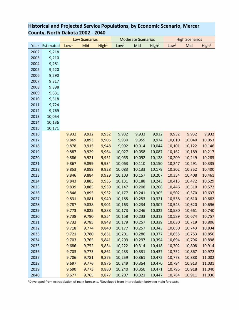
Historical and Projected Service Populations, by Economic Scenario, Mercer County, North Dakota 2002 ‐ 2040



2002 9,218

2003 9,210

2004 9,281

2005 9,220

2006 9,290

2007 9,317

2008 9,398

2009 9,631

2010 9,518

2011 9,724

2012 9,769

2013 10,054

2014 10,136

2015 10,171

2016 9,932 9,932 9,932 9,932 9,932 9,932 9,932 9,932 9,932

2017 9,869 9,893 9,905 9,930 9,959 9,974 10,010 10,040 10,053

2018 9,878 9,915 9,948 9,992 10,014 10,044 10,101 10,122 10,146

2019 9,887 9,929 9,964 10,027 10,058 10,087 10,162 10,189 10,217

2020 9,886 9,921 9,951 10,055 10,092 10,128 10,209 10,249 10,285

2021 9,867 9,899 9,934 10,063 10,110 10,150 10,247 10,291 10,335

2022 9,853 9,888 9,928 10,083 10,133 10,179 10,302 10,352 10,400

2023 9,846 9,884 9,929 10,103 10,157 10,207 10,354 10,408 10,461

2024 9,843 9,885 9,935 10,131 10,188 10,243 10,413 10,472 10,529

2025 9,839 9,885 9,939 10,147 10,208 10,268 10,446 10,510 10,572

2026 9,848 9,895 9,952 10,177 10,241 10,305 10,502 10,570 10,637

2027 9,831 9,881 9,940 10,185 10,253 10,321 10,538 10,610 10,682

2028 9,787 9,838 9,901 10,163 10,234 10,307 10,543 10,620 10,696

2029 9,773 9,825 9,888 10,173 10,246 10,322 10,580 10,661 10,740

2030 9,738 9,790 9,854 10,158 10,233 10,312 10,589 10,674 10,757

2031 9,732 9,785 9,848 10,179 10,257 10,339 10,630 10,719 10,806

2032 9,718 9,774 9,840 10,177 10,257 10,343 10,650 10,743 10,834

2033 9,721 9,780 9,851 10,201 10,286 10,377 10,655 10,753 10,850

2034 9,703 9,765 9,841 10,209 10,297 10,394 10,694 10,796 10,898

2035 9,686 9,752 9,834 10,222 10,314 10,418 10,702 10,808 10,914

2036 9,703 9,773 9,861 10,233 10,331 10,437 10,752 10,867 10,972

2037 9,706 9,781 9,875 10,259 10,361 10,472 10,773 10,888 11,002

2038 9,697 9,776 9,876 10,249 10,354 10,470 10,794 10,913 11,031

2039 9,690 9,773 9,880 10,240 10,350 10,471 10,795 10,918 11,040


Historical and Projected Service Populations, by Economic Scenario, McKenzie County, North Dakota 2002 ‐ 2040



2002 6,763

2003 6,769

2004 6,873

2005 6,901

2006 6,938

2007 7,031

2008 7,223

2009 7,344

2010 8,060

2011 8,777

2012 10,214

2013 11,099

2014 12,118

2015 11,792

2016 11,044 11,045 11,045 11,045 11,045 11,045 11,045 11,045 11,045

2017 10,752 11,031 11,081 11,243 11,358 11,435 11,538 11,646 11,749

2018 10,917 11,116 11,211 11,496 11,626 11,755 11,967 12,102 12,240

2019 11,101 11,223 11,347 11,789 11,971 12,094 12,322 12,506 12,608

2020 11,226 11,370 11,519 11,962 12,165 12,317 12,612 12,805 12,972

2021 11,294 11,451 11,612 12,070 12,289 12,466 12,768 12,975 13,172

2022 11,458 11,627 11,802 12,280 12,515 12,717 13,010 13,238 13,455

2023 11,800 11,993 12,193 12,672 12,929 13,160 13,476 13,733 13,980

2024 11,989 12,202 12,426 12,901 13,176 13,433 13,762 14,045 14,317

2025 12,143 12,377 12,624 13,096 13,390 13,673 14,008 14,316 14,613

2026 12,323 12,573 12,837 13,321 13,632 13,938 14,311 14,647 14,971

2027 12,446 12,711 12,990 13,491 13,819 14,149 14,545 14,907 15,256

2028 12,663 12,947 13,245 13,767 14,116 14,474 14,901 15,292 15,671

2029 12,732 13,020 13,322 13,876 14,236 14,610 15,073 15,484 15,882

2030 12,821 13,116 13,425 14,008 14,381 14,772 15,266 15,698 16,118

2031 12,868 13,168 13,481 14,097 14,481 14,887 15,417 15,868 16,307

2032 12,958 13,273 13,602 14,232 14,633 15,063 15,613 16,089 16,551

2033 13,048 13,386 13,740 14,368 14,789 15,248 15,808 16,312 16,802

2034 13,099 13,459 13,838 14,459 14,896 15,382 15,946 16,472 16,984

2035 13,157 13,545 13,955 14,562 15,021 15,533 16,093 16,637 17,175

2036 13,232 13,651 14,096 14,698 15,183 15,722 16,273 16,839 17,400

2037 13,310 13,761 14,240 14,837 15,347 15,914 16,458 17,047 17,631

2038 13,387 13,869 14,382 14,972 15,507 16,102 16,635 17,248 17,855

2039 13,490 14,006 14,555 15,137 15,699 16,323 16,850 17,487 18,119

2040 13,534 14,079 14,660 15,232 15,817 16,467 16,986 17,644 18,297

Historical and Projected Service Populations, by Economic Scenario, Renville County, North Dakota 2002 ‐ 2040



2002 2,593

2003 2,603

2004 2,559

2005 2,532

2006 2,539

2007 2,535

2008 2,447

2009 2,439

2010 2,550

2011 2,555

2012 2,667

2013 2,683

2014 2,657

2015 2,648

2016 2,643 2,643 2,643 2,643 2,643 2,643 2,643 2,643 2,643

2017 2,594 2,605 2,612 2,635 2,636 2,645 2,668 2,685 2,708

2018 2,583 2,595 2,609 2,653 2,673 2,690 2,725 2,746 2,764

2019 2,596 2,614 2,628 2,684 2,701 2,723 2,788 2,812 2,833

2020 2,599 2,618 2,634 2,711 2,731 2,749 2,832 2,853 2,870

2021 2,608 2,620 2,638 2,739 2,754 2,773 2,850 2,879 2,901

2022 2,609 2,623 2,643 2,744 2,765 2,783 2,871 2,896 2,918

2023 2,605 2,620 2,643 2,749 2,769 2,792 2,876 2,902 2,920

2024 2,609 2,625 2,650 2,759 2,772 2,794 2,889 2,914 2,939

2025 2,613 2,629 2,656 2,762 2,778 2,797 2,898 2,922 2,941

2026 2,608 2,625 2,654 2,765 2,780 2,798 2,905 2,927 2,949

2027 2,608 2,627 2,656 2,765 2,785 2,804 2,910 2,935 2,960

2028 2,606 2,626 2,651 2,763 2,786 2,806 2,916 2,945 2,970

2029 2,610 2,623 2,648 2,765 2,787 2,807 2,921 2,951 2,981

2030 2,604 2,624 2,647 2,770 2,792 2,808 2,931 2,960 2,988

2031 2,599 2,620 2,642 2,773 2,795 2,809 2,942 2,970 2,997

2032 2,598 2,620 2,642 2,777 2,799 2,814 2,951 2,978 3,004

2033 2,597 2,621 2,645 2,780 2,802 2,819 2,961 2,986 3,012

2034 2,596 2,619 2,647 2,782 2,806 2,824 2,966 2,991 3,015

2035 2,601 2,624 2,649 2,794 2,815 2,837 2,986 3,007 3,028

2036 2,602 2,625 2,650 2,799 2,822 2,845 2,996 3,018 3,039

2037 2,601 2,624 2,650 2,802 2,827 2,849 3,004 3,026 3,049

2038 2,604 2,628 2,651 2,810 2,836 2,860 3,014 3,037 3,059

2039 2,608 2,631 2,653 2,817 2,845 2,869 3,026 3,049 3,072


Historical and Projected Service Populations, by Economic Scenario, Slope County, North Dakota 2002 ‐ 2040



2002 759

2003 760

2004 758

2005 748

2006 758

2007 786

2008 771

2009 745

2010 752

2011 756

2012 819

2013 830

2014 826

2015 809

2016 816 816 816 816 816 816 816 816 816

2017 819 820 821 824 826 827 829 832 836

2018 822 824 826 832 835 837 843 846 850

2019 825 827 830 838 843 847 854 859 865

2020 827 831 835 844 851 856 863 870 879

2021 826 830 835 845 855 859 867 874 885

2022 825 831 836 846 857 861 869 879 891

2023 824 831 838 847 858 863 872 883 895

2024 823 832 839 848 860 866 876 886 897

2025 824 832 838 848 861 868 880 889 900

2026 823 831 838 847 861 869 881 890 905

2027 820 829 836 848 860 869 882 891 908

2028 818 828 836 848 859 868 882 893 909

2029 817 825 834 847 859 868 882 893 909

2030 813 823 832 847 858 868 882 893 909

2031 811 820 832 845 857 866 881 894 910

2032 810 818 830 845 857 866 881 895 911

2033 808 816 828 843 855 865 881 894 912

2034 805 814 826 842 854 865 881 895 913

2035 803 814 825 841 855 866 883 895 915

2036 802 813 823 839 854 865 882 895 916

2037 800 811 822 837 854 865 882 896 916

2038 797 809 822 836 853 865 882 896 917

2039 796 808 821 834 852 864 881 895 917

2040 795 807 819 832 851 863 881 894 917 1Developed from extrapolation of main forecasts. 2Developed from interpolation between main forecasts.

Historical and Projected Service Populations, by Economic Scenario, Stark County, North Dakota 2002 ‐ 2040



2002 23,393

2003 23,341

2004 23,582

2005 23,586

2006 23,773

2007 24,269

2008 24,831

2009 25,135

2010 26,282

2011 27,828

2012 31,089

2013 33,268

2014 35,998

2015 35,554

2016 33,946 33,946 33,946 33,946 33,946 33,946 33,946 33,946 33,946

2017 33,911 33,995 34,079 34,206 34,569 35,199 35,388 35,738 36,253

2018 33,993 34,385 34,777 35,396 36,436 37,410 38,588 38,997 39,656

2019 34,780 35,306 35,833 36,900 37,790 39,227 40,924 41,707 42,739

2020 35,536 36,051 36,613 37,777 39,140 40,840 42,430 43,688 44,665

2021 36,036 36,631 37,228 38,858 39,966 42,161 43,755 44,804 46,362

2022 36,331 36,901 37,621 39,391 40,786 42,804 44,361 45,877 47,268

2023 36,464 37,176 37,891 39,741 41,426 43,153 44,804 46,400 47,939

2024 36,581 37,425 38,272 40,191 41,959 43,546 45,263 46,948 48,632

2025 36,685 37,655 38,628 40,352 42,245 43,955 45,726 47,530 49,331

2026 36,649 37,668 38,690 40,360 42,336 44,129 46,069 47,979 49,887

2027 36,617 37,682 38,752 40,403 42,477 44,367 46,416 48,432 50,446

2028 36,585 37,699 38,817 40,453 42,625 44,612 46,777 48,898 51,018

2029 36,466 37,540 38,618 40,420 42,644 44,683 47,013 49,214 51,414

2030 36,380 37,437 38,499 40,423 42,709 44,811 47,286 49,571 51,857

2031 36,297 37,326 38,357 40,441 42,782 44,939 47,561 49,923 52,285

2032 36,317 37,397 38,482 40,555 42,988 45,233 47,948 50,405 52,863

2033 36,406 37,605 38,808 40,873 43,311 45,684 48,438 51,013 53,589

2034 36,498 37,818 39,142 41,132 43,623 46,123 48,919 51,613 54,300

2035 36,643 38,125 39,613 41,512 44,042 46,675 49,478 52,284 55,089

2036 36,773 38,410 40,052 42,022 44,477 47,234 50,025 52,934 55,844

2037 36,916 38,710 40,509 42,460 44,925 47,807 50,591 53,605 56,622

2038 37,066 39,016 40,973 42,786 45,377 48,388 51,156 54,279 57,404

2039 37,221 39,331 41,447 43,260 45,824 48,964 51,726 54,958 58,192

2040 37,428 39,698 41,976 43,856 46,332 49,605 52,360 55,705 59,051

Historical and Projected Service Populations, by Economic Scenario, Ward County, North Dakota 2002 ‐ 2040



2002 60,282

2003 59,896

2004 59,689

2005 60,097

2006 60,109

2007 61,023

2008 61,511

2009 62,179

2010 65,505

2011 68,413

2012 70,568

2013 73,714

2014 75,252

2015 75,166

2016 74,894 74,894 74,894 74,894 74,894 74,894 74,894 74,894 74,894

2017 74,480 74,622 74,764 76,018 76,163 76,308 77,014 77,169 77,323

2018 73,870 74,240 74,612 77,041 77,428 77,816 79,221 79,628 80,035

2019 74,045 74,599 75,157 78,104 78,692 79,281 81,084 81,704 82,323

2020 74,759 75,288 75,820 79,201 79,766 80,330 82,663 83,261 83,858

2021 75,415 76,088 76,766 79,995 80,714 81,434 83,833 84,596 85,359

2022 76,154 76,732 77,313 80,872 81,558 82,176 84,726 85,382 86,038

2023 76,439 77,062 77,685 81,231 81,893 82,555 85,571 86,277 86,983

2024 76,725 77,389 78,053 81,634 82,341 83,048 86,109 86,864 87,618

2025 77,009 77,715 78,421 82,080 82,832 83,584 86,323 87,123 87,923

2026 77,233 77,981 78,728 82,267 83,063 83,859 86,555 87,401 88,247

2027 77,469 78,259 79,048 82,458 83,298 84,138 86,804 87,697 88,590

2028 77,695 78,526 79,357 82,569 83,453 84,336 87,363 88,306 89,250

2029 77,855 78,728 79,600 82,843 83,772 84,700 87,772 88,764 89,757

2030 78,031 78,945 79,860 83,042 84,016 84,989 88,024 89,064 90,105

2031 78,247 79,204 80,161 83,482 84,503 85,524 88,737 89,832 90,926

2032 78,573 79,574 80,575 83,869 84,938 86,006 89,252 90,398 91,545

2033 78,911 79,957 81,004 84,207 85,323 86,440 89,836 91,036 92,236

2034 79,209 80,300 81,391 84,810 85,977 87,145 90,345 91,598 92,852

2035 79,582 80,719 81,856 85,322 86,541 87,760 91,226 92,538 93,851

2036 80,042 81,227 82,411 86,087 87,361 88,635 92,071 93,443 94,815

2037 80,500 81,733 82,965 86,840 88,170 89,500 93,027 94,461 95,896

2038 80,937 82,218 83,499 87,595 88,981 90,368 93,728 95,222 96,715

2039 81,349 82,678 84,008 88,292 89,736 91,179 94,567 96,123 97,679


Historical and Projected Service Populations, by Economic Scenario, Williams County, North Dakota 2002 ‐ 2040



2002 20,180

2003 20,265

2004 20,208

2005 20,102

2006 20,319

2007 21,109

2008 21,839

2009 22,388

2010 24,814

2011 29,760

2012 37,467

2013 42,148

2014 47,231

2015 45,312

2016 38,276 38,276 38,276 38,276 38,276 38,276 38,276 38,276 38,276

2017 38,622 38,949 39,351 39,625 39,858 40,224 41,691 42,388 43,194

2018 38,862 39,412 39,955 40,361 40,858 41,759 43,544 44,666 45,778

2019 39,101 39,974 40,557 41,104 41,888 42,856 44,964 46,591 48,697

2020 39,338 40,371 41,157 41,927 42,707 44,006 46,222 48,174 50,679

2021 39,541 40,831 42,001 42,853 43,773 45,357 47,808 50,293 52,823

2022 39,521 41,215 42,457 43,692 44,610 46,727 49,685 52,338 55,124

2023 39,414 41,301 43,104 44,292 45,308 47,609 51,689 54,528 57,567

2024 39,186 41,111 43,211 44,570 46,081 49,279 53,201 56,338 59,431

2025 38,962 40,934 43,502 44,927 46,996 50,405 54,809 58,138 61,417

2026 38,924 40,955 43,503 45,013 47,389 51,004 56,517 60,097 63,616

2027 38,875 41,086 43,686 45,475 47,937 51,783 57,586 61,369 65,078

2028 39,093 41,453 44,207 45,622 48,554 52,404 58,322 62,284 66,160

2029 39,081 41,606 44,517 46,073 49,160 53,039 58,836 62,974 67,020

2030 38,954 41,619 44,664 46,605 49,854 53,771 59,660 63,851 68,212

2031 38,722 41,540 44,730 46,867 50,269 54,212 59,943 64,446 68,841

2032 38,820 41,681 45,007 47,378 50,933 54,899 60,444 65,095 69,636

2033 39,175 42,053 45,502 48,221 51,926 55,454 61,118 65,911 70,584

2034 39,421 42,413 45,964 48,565 52,346 55,948 61,799 66,719 71,511

2035 39,822 42,953 46,635 48,808 52,661 56,343 62,601 67,647 72,563

2036 40,222 43,308 47,142 49,140 53,131 56,953 62,816 67,968 72,995

2037 40,377 43,708 47,693 49,887 54,060 58,066 63,336 68,620 73,777

2038 41,001 43,803 47,891 50,443 54,766 58,929 64,030 69,455 74,765

2039 41,201 44,149 48,363 50,999 55,467 59,780 64,705 70,274 75,725

2040 41,204 44,214 48,521 51,121 55,685 60,097 65,373 71,078 76,669

Documents

Power Forecast 2019: Williston Basin Oil and Gas Related ... Forecast 2019.pdf · 234 West Century Avenue Bismarck, ND 58503 701.255.5460 Power Forecast 2019: Williston Basin Oil