Embed Size (px)
Citation preview
sustainability
Article
Poverty Traps in the Municipalities of Ecuador:Empirical Evidence
Ronny Correa-Quezada 1 , Diego Fernando García-Vélez 1 ,María de la Cruz del Río-Rama 2,* and José Álvarez-García 3
1 Department of Economics, Universidad Técnica Particular de Loja (UTPL), Loja 11-01-608, Ecuador;[email protected] (R.C.-Q.); [email protected] (D.F.G.-V.)
2 Business Organisation and Marketing Department, Faculty of Business Administration and Tourism,University of Vigo, 32004 Ourense, Spain
3 Financial Economy and Accounting Department, Faculty of Finance, Business and Tourism,University of Extremadura, 10071 Caceres, Spain; [email protected]
* Correspondence: [email protected]; Tel.: +34-988-368-727
Received: 16 October 2018; Accepted: 16 November 2018; Published: 21 November 2018 �����������������
Abstract: The objective of this research is to identify from a spatial and temporal perspectivethe territories that are located in a “poverty trap” scenario. This is a scenario that does notallow overcoming the conditions and determinants that gave rise to this precarious situation,creating a vicious circle where the conditions of poverty endure through time. The methodologyapplied is an exploratory analysis of spatial dependence through Moran’s scatterplot and localindicators of spatial association (LISA) maps to visualize the spatial clusters of poverty. The databaseused is that of the population and housing censuses of 1990, 2001, and 2010 at the cantonal level.The results determine that 73 cantons were in a poverty trap over the period 1990–2001, while from2001–2010, there were 75 cantons in this situation, which were located mainly in the provinces ofEsmeraldas, Manabí, and Loja.
Keywords: poverty trap; unsatisfied basic needs (UBN); spatial clusters; exploratory spatial dataanalysis; Ecuador
1. Introduction
Regional inequalities in Ecuador’s economic development processes are noticeably revealedthrough a series of situations and conditions such as an economic and population concentration incertain provinces, disparities in the gross domestic product per capita, family income, access to publicservices, schooling, significant gaps in the provision of infrastructure, as well as the marginalizationand poverty of a considerable number of people in the population.
Poverty rates are proof of the disparities existing at the regional level in Ecuador, as argued byChiriboga and Wallis [1] and García-Vélez [2], who observed that the poverty rates differ significantlyfor each region. The common factor in these two investigations is that the regions with the lowestlevels of poverty are those that concentrate economic, political, and administrative activities; while theregions with the highest poverty are those of the Ecuadorian Amazon.
Interest in issues related to the study of poverty, including its causes and consequences, emerged inEcuador in the 1970s, with the rise of territorial planning. The government started these initiativesthrough the National Planning Board (JUNAPLA) in view of the need to focus and prioritize socialspending toward satisfying the basic needs of the lowest income sectors. In this sense, Ruiz andSánchez [3] pointed out that this institution developed several studies on living conditions, housing,and access to services in working-class neighborhoods where marginalization is clearly evident.
Sustainability 2018, 10, 4316; doi:10.3390/su10114316 www.mdpi.com/journal/sustainability
Sustainability 2018, 10, 4316 2 of 18
One of the first academic investigations on the satisfaction of basic needs was carried out byBarreiros et al. [4]. These authors reiterated the need to follow an integrated development approach toeradicate poverty, included the basic needs approach in the development agenda, and emphasized theinteraction between poverty and the economic, social, and political structures. Subsequently, Cobos [5]stated that the persistence of socio-territorial inequalities and their relationship with local developmentis based on factors not only inherent to the territory, such as natural or climatic issues, but also on social,economic, and/or political issues. In 2009, Skoufias and López-Acevedo [6] prepared a report forIBRD-World Bank [7] on territorial disparities in Latin America; according to Boisier [8], this is one ofthe most important reports. In the case of Ecuador, the authors stated that there are greater differencesin the poverty rates between urban and rural areas than between regions in general. Subsequently,Scott and Janikas [9] developed a map of poverty clusters for Ecuador using Moran’s index, and foundhigh poverty clusters in the north and south of the country. The contribution of this work is notanalytical, because the approach of the authors’ work was defined by the use of tools and software formapping and spatial analysis, and was not focused on poverty issues.
Béland and Escobar [10], based on population and housing censuses, living conditions surveys,and other official publications, carried out a socioeconomic characterization that includes 10 parishes inthe province of Tungurahua (located in the central Ecuadorian sierra). These authors found that povertyby consumption levels is very high, but poverty with unsatisfied basic needs (UBN) is even higher,which is linked to those territories that are highly dependent on agricultural production activities,with discrete productive diversification and apparent modest economic flows. Burgos [11] analyzedbehavior due to UBN and the relationship between economic growth and its main components,and also formulated a simulation on the effects that would be generated on the poverty indicator dueto UBN if all of the households in the country were connected to the public drinking water supply andsewage disposal systems. As a result of the simulations carried out, a sharp drop in the magnitudes ofpoverty and extreme poverty indicators with UBN were observed, especially in rural areas and theMontubia and Afro-Ecuadorian indigenous ethnic groups.
At the state level, the System of Social Indicators of Ecuador [12] developed the poverty indicatorwith UBN and the extreme poverty indicator with UBN. According to the former, in 1990, 79.6% ofthe total Ecuadorian population lived in poverty; in 2001, this figure was 71.4%, and according tothe last national census carried out in 2010, it was 60.1%, that is, approximately 8,605,803 peoplewere in structural poverty conditions that did not allow them to satisfy minimum subsistence needs.The second indicator shows lower results, since in order for a household to be considered in extremepoverty, it must not satisfy at least two basic needs. So, for 1990, 51.8% of the population suffered fromextreme poverty due to UBN; in 2001, this figure was 39.9%, and finally, in 2010, 26.8% of extremepoverty was identified. This brief analysis reports a significant decrease in poverty and extreme povertywith UBN. However, this progress has been uneven in the Ecuadorian territory. As Cobos [5] pointedout, the poverty percentages in urban and rural areas between regions showed a large inequalitybetween the areas of the same territorial district, where the greatest difference was more than 40 pointsin the Ecuadorian Sierra. This situation exemplifies the problem of poverty, as well as that of inequalitywithin the same territorial jurisdiction.
In this area, according to the Ministerio de Coordinación de Desarrollo Social [13], several studieshave been carried out that have analyzed the distribution of spatial poverty, which combine severalmethodological strategies to describe the existing inequalities among the geographic units of Ecuador.The following studies are included:
(1) The Economic Commission for Latin America and the Caribbean [14] presents the levels ofpoverty measured by UBN at the cantonal and parochial levels, based on data from the IVNational Population Census and Housing III of 1982.
(2) The National Development Council [15] develops a consolidated national map of poverty thatsynthesizes in a composite cantonal index the result of several spatial studies related to poverty.
Sustainability 2018, 10, 4316 3 of 18
(3) The National Institute of Statistics and Census [16] shows a summary of UBN of the Ecuadorianpopulation that incorporates variables of infrastructure, education, and health, which arecalculated on the basis of the Population and Housing Census of 1990.
(4) The Technical Secretariat of the Social Front [17] estimates a model that projects the per capitafamily consumption of the Living Conditions Survey of 1994 and the 1990 Population andHousing Census.
(5) The Office of Planning of the Presidency of the Republic [18], which is based on the previousstudy and the Living Conditions Survey of 1995, incorporated socioeconomic variables in theestimation of regression models, correlating it with household consumption.
(6) The World Bank and the System of Social Indicators of Ecuador (SIISE) [7] developed a povertymap and an econometric model based on an indicator of poverty or inequality at household level,with data from the censuses of 1990, 2001, and the surveys of living conditions for the years 1994and 1999.
(7) SIISE-STMCDS [19], Secretaría Técnica del Ministerio de Coordinación de Desarrollo Social(STMCDS) developed a poverty map that shows information on poverty indicators forconsumption and inequality, disaggregated at cantonal and parochial level. It is based onthe 2005–2006 Living Conditions Surveys and the Population Census of 2001.
(8) The SIISE [20] shows poverty maps by UBN at the provincial, cantonal, and parochial levels ata descriptive level, based on information from the 1990, 2001, and 2010 censuses.
(9) The National Secretariat for Planning and Development [21] presents the atlas of socioeconomicinequalities in Ecuador, which explains a typology of territories according to their socialconditions, and carries out a historical (20 years) and territorialized analysis of the differenttypes of inequality (education, health, housing, decent employment, gender-based violence,and child abuse) that have existed and are still present in the country.
In this context, the objective of this research is to identify from a spatial and temporal perspectivethose territories that are located in a “poverty trap” scenario. To achieve the proposed objective,the methodology used is exploratory spatial data analysis (ESDA) and its spatial association techniques;Moran’s scatterplot, LISA graphs (local indicators of spatial association), and dynamic maps for presentingthe results. Unlike the aforementioned studies, in this work, the ESDA technique is used to visualizespatial distributions, detect atypical locations, and verify the existence of spatial association patterns,which enables identifying if there is spatial autocorrelation of poverty or if it is distributed randomlythroughout territories and time. The unsatisfied basic needs (UBN) approach is followed, mainly becauseit provides data with a high level of disaggregation that is perfectly comparable over time.
The present investigation contributes with innovative questions when using procedures andtools that, through the use and treatment of spatial data, incorporate the characteristics, dynamics,and behaviors of the processes related to the basic needs of the population in the municipalities ofEcuador. In addition, its application shows territorial relationships, which enables the provision ofadditional knowledge on the subject in question. This analysis can be applied to other variablesof a different nature to address the problems in a way that allows discovering the singularities ofthe territories of a phenomenon to define their participation within the global context. In addition,the focus of this work will allow researchers and public policy managers to better understand povertyfrom a new perspective: spatial. This in turn, increases the knowledge of the regional economic realityof the country, and would enable a better design of regional development policies.
This article is structured in five sections. In the introduction, the object of the study is contextualized,and the objective is stated. Hereafter, the term “poverty traps”, is defined and the indicators that measureit are mentioned. In the methodology section, the analysis variable is presented in this research, as well asthe statistical tool used, ESDA, and the results obtained are included in the following epigraph. Finally,the conclusions are discussed.
Sustainability 2018, 10, 4316 4 of 18
2. Conceptual Framework
2.1. Poverty Traps
A poverty trap is conceived as a situation in which a household cannot leave the precariousenvironment in which it lives, either due to internal household reasons or external reasons such asa lack of government support to improve its quality of life. Banerjee and Duflo [22] considered that thefuture income of a poor household will be lower than its current income, so people will become poorerover time, which places them in a poverty trap.
Therefore, households that face poverty traps are those that systematically show difficulties toachieve minimum levels of well-being over time, and therefore are subject to situations of persistentdeprivation [23]. This situation is caused by the existence of multiple and dynamic factors, which arethe subject of study and analysis among researchers and those who design public policies [24,25].
Several studies warn of the presence of poverty traps in different countries and their directrelationship with the deprivation of access to educational and formative levels [26–30], both for thehead of the family and the household members. Meanwhile, the accumulation of goods generatesdynamics that persistently traps households with lower possession levels of these goods below thepoverty line [30,31].
Poverty traps are not generated only by conditions specific to households, but also by thehouseholds that surround them. In this sense, considering the neighborhood effects, stated that “livingin a poor neighborhood can increase the adverse consequences of poverty, and reduces the chances ofgetting out of that situation” [32] (p. 1). Thus, if poverty traps are subject to the neighborhood wherethe household is located, the geographical location of households can be considered a condition thatprovides a greater capacity to explain changes in the incidence and persistence of poverty.
In effect, those territories trapped in different poverty dimensions have similar characteristics:their high rurality [33–36], their distance from the administrative and commercial capitals [37],and structural factors such as difficult access to their territories [38]. In addition, the poverty intensity,the education deprivation gap, and the deepest entrapment occurs in those territories where themajority of the population is indigenous [38,39].
2.2. Measures of Poverty
In the study of poverty, there are numerous conceptualizations, approaches, and measures toidentify individuals that are considered poor in a given society. The following are included in the mostprominent approaches: biological [40], relative deprivation [41,42], economic [43–45], unsatisfied basicneeds [46,47], capacities [48], and multidimensional [49,50].
However, no approach can be considered as the most appropriate for measuring poverty.Therefore, the decision of which approach to follow is highly dependent on the measurement intentionsand the availability of information. Therefore, the starting point is to establish the indicator that will beused to measure poverty. Specifically, the academic literature shows a wide variety of measures [51–53],choosing to measure poverty in terms of unsatisfied basic needs (UBN) for this research. In Ecuador,it is the measure that shows data with the greatest regional disaggregation and allows fulfilling theobjective of identifying those territories that continue in a “poverty trap” scenario. In this sense,the cantons that relapse in this situation of poverty during the period 1990–2010 will be locatedspatially; in addition, the presence of spatial autocorrelation and the formation of clusters will beverified, taking as reference the data of the extreme poverty index with homogenized UBN at thecantonal level available in the national censuses of 1990, 2001, and 2010. With reference to the term“cantons”, these are the political-administrative units through which work is done in this investigation,which refer to the Administrative Political Division of Ecuador; nine planning areas, 24 provinces,221 cantons, and 1149 parishes.
The UBN approach is a contribution of the Economic Commission for Latin America and theCaribbean (ECLAC), which was introduced in the 1980s, and is used exclusively in Latin America
Sustainability 2018, 10, 4316 5 of 18
for the poverty measure based on census information. This approach “consists of verifying whetherhouseholds have satisfied a series of previously established needs and considers those that have notachieved them as poor” [54] (p. 24). It is also known as a direct method for measuring poverty, since itdetermines whether the population actually satisfies their basic needs.
The basic needs that the approach considers depend on the availability of information. However,the different applications of the approach include four basic needs: economic capacity, accessto adequate health services, access to basic education, and access to adequate housing [54–56],among others. The UBN indicator for Ecuador officially measured by the National Institute of Statisticsand Census (INEC), considers precisely the four basic needs mentioned.
3. Methodology
3.1. Analysis Variable: Extreme Poverty Rate with UBN
The variable that will be used in this research is the extreme poverty rate with unsatisfied basicneeds (UBN) at the cantonal level, which was calculated from the population and housing censuses of1990, 2001, and 2010. The extreme poverty rate is the number of people living in conditions of extremepoverty, which is expressed as the total population of the canton in a given year.
The data are obtained from the System of Social Indicators of Ecuador (SIISE). This variable isconsidered to identify poverty traps in Ecuador, because it conveys a multidimensional vision of poverty,in addition to enabling studying poverty over time and at a higher level of regional disaggregation.
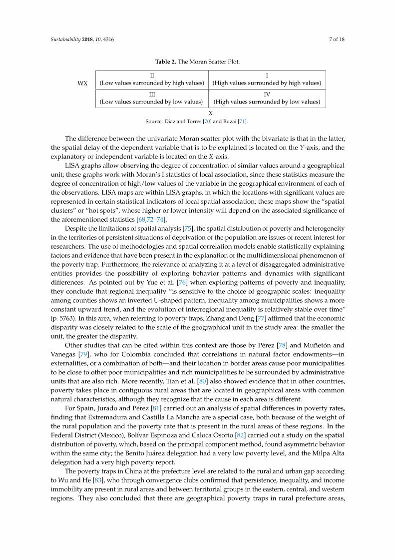
In Ecuador, the extreme poverty rate with UBN is calculated based on five dimensions or basicneeds, distributed in eight indicators that measure the concept of “deprivation”. In this sense,households that are deprived in two or more indicators are considered in extreme poverty (see Table 1).
According to the 1990 census, there were 218 cantons in Ecuador; in 2001, the number of cantonsincreased to 220, and in the 2010 census, there were 221 cantons and three non-delimited zones.This variation occurs due to four reasons: (1) the creation of new cantons; (2) the division of cantons;(3) parishes that are created in new cantons; and (4) the creation of new provinces with their respectivecantons. As a consequence of the variation in the number of cantons, it is necessary to homogenizegeographically the series so that the data are comparable.
Table 1. Dimensions and indicators of unsatisfied basic needs (UBN).
Dimensions Deprivation Indicators
Economic capacity If the years of schooling of the head of the family are less than or equal to two years.If there are more than three people for each person employed in the home.
Access to basic education If there are children at home aged between six and 12 who do not attend school.
Access to housing If the floor material of the house is with earth or other materials.If the wall material of the house is made of reed, matting, or other materials.
Access to basic servicesIf the house does not have a toilet or if it has one, it is a concrete pit or latrine.If the water obtained by the house is not from a public network or another piping source.
Overcrowding If the number of people per bedroom is greater than three.
Source: Prepared by the National Institute of Statistics and Censuses (INEC) of Ecuador [16].
The process of homogenization consists of putting together a series with the same number of cantonsfor each census, for which the cantonal structure of the 2010 census is taken as a reference, since it isnecessary to perform the analyses and the calculation of indicators based on the political-administrativeorganization in force in the country. Of the 221 current cantons, 2.7% (six) are newly created, 2.2% (five)are cantons that underwent modifications, and 95.1% (213) have not undergone alterations since 1990,for which only 4.9% (11) of cantons were homogenized. In addition to the 221 cantons, there are threenon-delimited zones; so, the research is developed considering 224 study units.
Sustainability 2018, 10, 4316 6 of 18
3.2. Spatial Analysis of Poverty
ESDA is used to identify systematic relationships between variables when the relationshipbetween them is unclear. According to Tukey ([57] cited by Yrigoyen [58]), this multivariate analysiscan be defined as “the set of graphic and descriptive tools used to discover behavior patterns in thedata and to establish the hypotheses with the smallest possible structure”. Anselin [59] defined itas the set of techniques that describe and visualize spatial distributions, identify “spatial outliers”,discover spatial association outlines, such as “clusters” or “hot spots”, and suggest spatial structuresor other forms of spatial heterogeneity. According to Yrigoyen [58], the ESDA must be the stage priorto any modeling and decision-making analysis in the field of socioeconomic research. Following thisline, the main spatial association techniques are used in this research: the dispersion diagram of Morán(univariate and bivariate) and LISA graphs. In addition, dynamic maps are used to show the results.The techniques mentioned and the maps are worked with using GeoDa 1.12 software.
Moran’s index [60] is one of the most used techniques to detect spatial autocorrelation betweenspatial units, and it is similar to the correlation coefficient between two variables [61]. According toBohórquez and Ceballos [62] (p. 22), this index is “an adaptation of a non-spatial correlation measureto a spatial context, and it is normally applied to spatial units where information is available in theform of ratios or intervals”. Moran’s I statistics is basically the Pearson correlation coefficient [63] witha user-defined weight matrix that maintains the range between −1 and 1 [64]:
I =NS0
∑i ∑j WijZiZj
∑i Z2i
(1)
where:N is the number of regions,Zi = Xi − X; therefore, it is X in terms of deviations from its mean,S0 = ∑
i∑j
Wij is the sum of the space weights, and
WijZi it is the spatial lag of Z.
For a better understanding, the index is standardized, and the Z (I) value is obtained. The valuestaken by this standardized index can be positive or negative. In the case that they are positive andstatistically significant, it is concluded that the data show positive spatial autocorrelation; if theyare negative and statistically significant, it is concluded that there is negative spatial autocorrelation.Moran’s index, which lacks spatial autocorrelation, should be close to zero [65].
According to Rivero [66] (p. 54), “although Moran’s I test is the most used in practice, there are,however, other alternatives to it, such as the Geary C test [67], or the Getis G test and Ord [68]”.
The ESDA “has various graphs that allow to visualize the presence or absence of spatialautocorrelation clearly and directly” [66] (p. 54), with the univariate Moran scatter plot being the mostused. It is represented on a Cartesian plane in which the previously standardized X variable is locatedon the X-axis and the spatial delay of the standardized WX variable is located on the Y-axis. The slopeof the regression line obtained from the spatial relationship is the Moran’s I statistical value of spatialautocorrelation [69]. The association presented in the diagram is divided into four categories: two forpositive spatial autocorrelation, and two for negative spatial autocorrelation. The positive ones areshown in quadrants I and III, and the negative ones are shown in quadrants II and IV. Positive spatialautocorrelation refers to high values of the variable surrounded by high values or low values of thevariable surrounded by low values, and negative spatial autocorrelation refers to high values of thevariable surrounded by low values, or low values of the variable surrounded by high values (Table 2).
Sustainability 2018, 10, 4316 7 of 18
Table 2. The Moran Scatter Plot.
WXII
(Low values surrounded by high values)I
(High values surrounded by high values)
III(Low values surrounded by low values)
IV(High values surrounded by low values)
XSource: Díaz and Torres [70] and Buzai [71].
The difference between the univariate Moran scatter plot with the bivariate is that in the latter,the spatial delay of the dependent variable that is to be explained is located on the Y-axis, and theexplanatory or independent variable is located on the X-axis.
LISA graphs allow observing the degree of concentration of similar values around a geographicalunit; these graphs work with Moran’s I statistics of local association, since these statistics measure thedegree of concentration of high/low values of the variable in the geographical environment of each ofthe observations. LISA maps are within LISA graphs, in which the locations with significant values arerepresented in certain statistical indicators of local spatial association; these maps show the “spatialclusters” or “hot spots”, whose higher or lower intensity will depend on the associated significance ofthe aforementioned statistics [68,72–74].
Despite the limitations of spatial analysis [75], the spatial distribution of poverty and heterogeneityin the territories of persistent situations of deprivation of the population are issues of recent interest forresearchers. The use of methodologies and spatial correlation models enable statistically explainingfactors and evidence that have been present in the explanation of the multidimensional phenomenon ofthe poverty trap. Furthermore, the relevance of analyzing it at a level of disaggregated administrativeentities provides the possibility of exploring behavior patterns and dynamics with significantdifferences. As pointed out by Yue et al. [76] when exploring patterns of poverty and inequality,they conclude that regional inequality “is sensitive to the choice of geographic scales: inequalityamong counties shows an inverted U-shaped pattern, inequality among municipalities shows a moreconstant upward trend, and the evolution of interregional inequality is relatively stable over time”(p. 5763). In this area, when referring to poverty traps, Zhang and Deng [77] affirmed that the economicdisparity was closely related to the scale of the geographical unit in the study area: the smaller theunit, the greater the disparity.
Other studies that can be cited within this context are those by Pérez [78] and Muñetón andVanegas [79], who for Colombia concluded that correlations in natural factor endowments—inexternalities, or a combination of both—and their location in border areas cause poor municipalitiesto be close to other poor municipalities and rich municipalities to be surrounded by administrativeunits that are also rich. More recently, Tian et al. [80] also showed evidence that in other countries,poverty takes place in contiguous rural areas that are located in geographical areas with commonnatural characteristics, although they recognize that the cause in each area is different.
For Spain, Jurado and Pérez [81] carried out an analysis of spatial differences in poverty rates,finding that Extremadura and Castilla La Mancha are a special case, both because of the weight ofthe rural population and the poverty rate that is present in the rural areas of these regions. In theFederal District (Mexico), Bolívar Espinoza and Caloca Osorio [82] carried out a study on the spatialdistribution of poverty, which, based on the principal component method, found asymmetric behaviorwithin the same city; the Benito Juárez delegation had a very low poverty level, and the Milpa Altadelegation had a very high poverty report.
The poverty traps in China at the prefecture level are related to the rural and urban gap accordingto Wu and He [83], who through convergence clubs confirmed that persistence, inequality, and incomeimmobility are present in rural areas and between territorial groups in the eastern, central, and westernregions. They also concluded that there are geographical poverty traps in rural prefecture areas,
Sustainability 2018, 10, 4316 8 of 18
and indicated the need for intervention through policies to reduce the urban–rural gap and eliminatepoverty traps; Tian et al. [80] agreed.
In short, the use of spatial data and the application of exploratory analysis techniques in thisresearch make a significant contribution to the study of living conditions and the subsistence of thepopulation, because they place census data from official sources in the space and at subnational(cantonal) scales. This allows obtaining a high level of reliability in the results, as well as a betterunderstanding of the spatial relationships that occur in the territory over time, and defining sets andsignificant common patterns of grouping.
4. Results
4.1. Persistence of Inequalities over Time
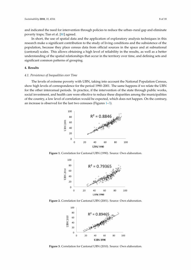
The levels of extreme poverty with UBN, taking into account the National Population Census,show high levels of correspondence for the period 1990–2001. The same happens if we relate the UBNfor the other intercensal periods. In practice, if the intervention of the state through public works,social investment, and health care were effective to reduce these disparities among the municipalitiesof the country, a low level of correlation would be expected, which does not happen. On the contrary,an increase is observed for the last two censuses (Figures 1–3).
Sustainability 2018, 10, x FOR PEER REVIEW 8 of 18
The levels of extreme poverty with UBN, taking into account the National Population Census, show high levels of correspondence for the period 1990–2001. The same happens if we relate the UBN for the other intercensal periods. In practice, if the intervention of the state through public works, social investment, and health care were effective to reduce these disparities among the municipalities of the country, a low level of correlation would be expected, which does not happen. On the contrary, an increase is observed for the last two censuses (Figures 1–3).
Figure 1. Correlation for Cantonal UBN (1990). Source: Own elaboration.
Figure 2. Correlation for Cantonal UBN (2001). Source: Own elaboration.
Figure 3. Correlation for Cantonal UBN (2010). Source: Own elaboration.
In this context, Serrano [84], when addressing issues related to public policy, investment by canton, and poverty reduction through the evolution of the UBN 2001–2010, pointed out the difficulty of incorporating public investment in the analysis due to information sources. A large proportion of expenditure is recorded and accounted for as national expenditure, and does not distinguish the province or the canton of investment; so, a direct correlation between public investment at the municipal level and a reduction of extreme poverty with UBN is not found. However, it is concluded that not having corroborated an effect of investment on the poverty indicator with UBN does not prove that the investment does not influence poverty.
4.2. Poverty Trap
Scatter diagrams and Moran’s index are used in order to see spatial interactions [85], as well as to verify the heterogeneity (systematic differences) and spatial dependence [86,87] that causes the
Figure 1. Correlation for Cantonal UBN (1990). Source: Own elaboration.
Sustainability 2018, 10, x FOR PEER REVIEW 8 of 18
The levels of extreme poverty with UBN, taking into account the National Population Census, show high levels of correspondence for the period 1990–2001. The same happens if we relate the UBN for the other intercensal periods. In practice, if the intervention of the state through public works, social investment, and health care were effective to reduce these disparities among the municipalities of the country, a low level of correlation would be expected, which does not happen. On the contrary, an increase is observed for the last two censuses (Figures 1–3).
Figure 1. Correlation for Cantonal UBN (1990). Source: Own elaboration.
Figure 2. Correlation for Cantonal UBN (2001). Source: Own elaboration.
Figure 3. Correlation for Cantonal UBN (2010). Source: Own elaboration.
In this context, Serrano [84], when addressing issues related to public policy, investment by canton, and poverty reduction through the evolution of the UBN 2001–2010, pointed out the difficulty of incorporating public investment in the analysis due to information sources. A large proportion of expenditure is recorded and accounted for as national expenditure, and does not distinguish the province or the canton of investment; so, a direct correlation between public investment at the municipal level and a reduction of extreme poverty with UBN is not found. However, it is concluded that not having corroborated an effect of investment on the poverty indicator with UBN does not prove that the investment does not influence poverty.
4.2. Poverty Trap
Scatter diagrams and Moran’s index are used in order to see spatial interactions [85], as well as to verify the heterogeneity (systematic differences) and spatial dependence [86,87] that causes the
Figure 2. Correlation for Cantonal UBN (2001). Source: Own elaboration.
Sustainability 2018, 10, x FOR PEER REVIEW 8 of 18
The levels of extreme poverty with UBN, taking into account the National Population Census, show high levels of correspondence for the period 1990–2001. The same happens if we relate the UBN for the other intercensal periods. In practice, if the intervention of the state through public works, social investment, and health care were effective to reduce these disparities among the municipalities of the country, a low level of correlation would be expected, which does not happen. On the contrary, an increase is observed for the last two censuses (Figures 1–3).
Figure 1. Correlation for Cantonal UBN (1990). Source: Own elaboration.
Figure 2. Correlation for Cantonal UBN (2001). Source: Own elaboration.
Figure 3. Correlation for Cantonal UBN (2010). Source: Own elaboration.
In this context, Serrano [84], when addressing issues related to public policy, investment by canton, and poverty reduction through the evolution of the UBN 2001–2010, pointed out the difficulty of incorporating public investment in the analysis due to information sources. A large proportion of expenditure is recorded and accounted for as national expenditure, and does not distinguish the province or the canton of investment; so, a direct correlation between public investment at the municipal level and a reduction of extreme poverty with UBN is not found. However, it is concluded that not having corroborated an effect of investment on the poverty indicator with UBN does not prove that the investment does not influence poverty.
4.2. Poverty Trap
Scatter diagrams and Moran’s index are used in order to see spatial interactions [85], as well as to verify the heterogeneity (systematic differences) and spatial dependence [86,87] that causes the
Figure 3. Correlation for Cantonal UBN (2010). Source: Own elaboration.

Sustainability 2018, 10, 4316 9 of 18
In this context, Serrano [84], when addressing issues related to public policy, investment bycanton, and poverty reduction through the evolution of the UBN 2001–2010, pointed out the difficultyof incorporating public investment in the analysis due to information sources. A large proportionof expenditure is recorded and accounted for as national expenditure, and does not distinguishthe province or the canton of investment; so, a direct correlation between public investment at themunicipal level and a reduction of extreme poverty with UBN is not found. However, it is concludedthat not having corroborated an effect of investment on the poverty indicator with UBN does not provethat the investment does not influence poverty.
4.2. Poverty Trap
Scatter diagrams and Moran’s index are used in order to see spatial interactions [85], as well asto verify the heterogeneity (systematic differences) and spatial dependence [86,87] that causes theindex of extreme poverty with UBN in cantons. For the calculation of the Moran’s index, a matrix offirst-order space weights was used, which allowed us to establish how the territorial units relate toeach other.
According to the dispersion diagrams, for the three census periods, most of the cantons are locatedin quadrants I and III (High–High and Low–Low, respectively), which show a spatial autocorrelationbetween extreme poverty conditions and UBN in Ecuador (Figures 4–6). In effect, Moran’s I issignificant (all three have a pseudo-probability of less than 1% that the spatial distribution is a randomphenomenon) and positive in each of them. This results in grouping neighboring cantons with highUBN, as well as the presence of adjoining cantons in which basic needs are better satisfied. In fact, it isevident that in Ecuador, there is a group of poor cantons surrounded by poor cantons, and non-poorcantons surrounded by non-poor cantons.
The appearance of clusters in the territory is due to the presence of spatial autocorrelation.The concept of cluster has its origin in the definition of the first law of geography of Tobler [88]:“everything is related to everything, but things close to each other are more related than distantones” (p. 236), while spatial autocorrelation occurs when similar characteristics or the behavior of thevariables in neighboring places are shown [86,89,90].
Sustainability 2018, 10, x FOR PEER REVIEW 9 of 18
index of extreme poverty with UBN in cantons. For the calculation of the Moran’s index, a matrix of first-order space weights was used, which allowed us to establish how the territorial units relate to each other.
According to the dispersion diagrams, for the three census periods, most of the cantons are located in quadrants I and III (High–High and Low–Low, respectively), which show a spatial autocorrelation between extreme poverty conditions and UBN in Ecuador (Figures 4–6). In effect, Moran’s I is significant (all three have a pseudo-probability of less than 1% that the spatial distribution is a random phenomenon) and positive in each of them. This results in grouping neighboring cantons with high UBN, as well as the presence of adjoining cantons in which basic needs are better satisfied. In fact, it is evident that in Ecuador, there is a group of poor cantons surrounded by poor cantons, and non-poor cantons surrounded by non-poor cantons.
The appearance of clusters in the territory is due to the presence of spatial autocorrelation. The concept of cluster has its origin in the definition of the first law of geography of Tobler [88]: “everything is related to everything, but things close to each other are more related than distant ones” (p. 236), while spatial autocorrelation occurs when similar characteristics or the behavior of the variables in neighboring places are shown [86,89,90].
Figure 4. The Moran Scatter Plot for Cantonal UBN (1990). Source: Own elaboration.
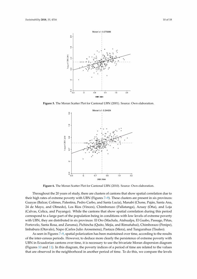
Figure 5. The Moran Scatter Plot for Cantonal UBN (2001). Source: Own elaboration.
Figure 4. The Moran Scatter Plot for Cantonal UBN (1990). Source: Own elaboration.
Sustainability 2018, 10, 4316 10 of 18
Sustainability 2018, 10, x FOR PEER REVIEW 9 of 18
index of extreme poverty with UBN in cantons. For the calculation of the Moran’s index, a matrix of first-order space weights was used, which allowed us to establish how the territorial units relate to each other.
According to the dispersion diagrams, for the three census periods, most of the cantons are located in quadrants I and III (High–High and Low–Low, respectively), which show a spatial autocorrelation between extreme poverty conditions and UBN in Ecuador (Figures 4–6). In effect, Moran’s I is significant (all three have a pseudo-probability of less than 1% that the spatial distribution is a random phenomenon) and positive in each of them. This results in grouping neighboring cantons with high UBN, as well as the presence of adjoining cantons in which basic needs are better satisfied. In fact, it is evident that in Ecuador, there is a group of poor cantons surrounded by poor cantons, and non-poor cantons surrounded by non-poor cantons.
The appearance of clusters in the territory is due to the presence of spatial autocorrelation. The concept of cluster has its origin in the definition of the first law of geography of Tobler [88]: “everything is related to everything, but things close to each other are more related than distant ones” (p. 236), while spatial autocorrelation occurs when similar characteristics or the behavior of the variables in neighboring places are shown [86,89,90].
Figure 4. The Moran Scatter Plot for Cantonal UBN (1990). Source: Own elaboration.
Figure 5. The Moran Scatter Plot for Cantonal UBN (2001). Source: Own elaboration. Figure 5. The Moran Scatter Plot for Cantonal UBN (2001). Source: Own elaboration.Sustainability 2018, 10, x FOR PEER REVIEW 10 of 18
Figure 6. The Moran Scatter Plot for Cantonal UBN (2010). Source: Own elaboration.
Throughout the 20 years of study, there are clusters of cantons that show spatial correlation due to their high rates of extreme poverty with UBN (Figures 7–9). These clusters are present in six provinces: Guayas (Balzar, Colimes, Palestina, Pedro Carbo, and Santa Lucia), Manabí (Chone, Paján, Santa Ana, 24 de Mayo, and Olmedo), Los Ríos (Vinces), Chimborazo (Pallatanga), Azuay (Oña), and Loja (Calvas, Celica, and Puyango). While the cantons that show spatial correlation during this period correspond to a large part of the population being in conditions with low levels of extreme poverty with UBN, they are distributed in six provinces: El Oro (Machala, Atahualpa, El Guabo, Passage, Piñas, Portovelo, Santa Rosa, and Zaruma), Pichincha (Quito, Mejía, and Rimuñahui), Chimborazo (Penipe), Imbabura (Otavalo), Napo (Carlos Julio Arosemena), Pastaza (Mera), and Tungurahua (Tisaleo).
As seen in figures 7–9, spatial polarization has been maintained over time, according to the results of the inter-census periods. However, to deduce more clearly the persistence of extreme poverty with UBN in Ecuadorian cantons over time, it is necessary to use the bivariate Moran dispersion diagram (Figures 10 and 11). In this diagram, the poverty indices of a period of time are related to the values that are observed in the neighborhood in another period of time. To do this, we compare the levels of poverty in a given year and location with the values observed in poverty lagged temporally and spatially [32].
Figure 7. Poverty clusters by municipalities in the year 1990. Source: Own elaboration.
Figure 6. The Moran Scatter Plot for Cantonal UBN (2010). Source: Own elaboration.
Throughout the 20 years of study, there are clusters of cantons that show spatial correlation due totheir high rates of extreme poverty with UBN (Figures 7–9). These clusters are present in six provinces:Guayas (Balzar, Colimes, Palestina, Pedro Carbo, and Santa Lucia), Manabí (Chone, Paján, Santa Ana,24 de Mayo, and Olmedo), Los Ríos (Vinces), Chimborazo (Pallatanga), Azuay (Oña), and Loja(Calvas, Celica, and Puyango). While the cantons that show spatial correlation during this periodcorrespond to a large part of the population being in conditions with low levels of extreme povertywith UBN, they are distributed in six provinces: El Oro (Machala, Atahualpa, El Guabo, Passage, Piñas,Portovelo, Santa Rosa, and Zaruma), Pichincha (Quito, Mejía, and Rimuñahui), Chimborazo (Penipe),Imbabura (Otavalo), Napo (Carlos Julio Arosemena), Pastaza (Mera), and Tungurahua (Tisaleo).
As seen in Figures 7–9, spatial polarization has been maintained over time, according to the resultsof the inter-census periods. However, to deduce more clearly the persistence of extreme poverty withUBN in Ecuadorian cantons over time, it is necessary to use the bivariate Moran dispersion diagram(Figures 10 and 11). In this diagram, the poverty indices of a period of time are related to the valuesthat are observed in the neighborhood in another period of time. To do this, we compare the levels

Sustainability 2018, 10, 4316 11 of 18
of poverty in a given year and location with the values observed in poverty lagged temporally andspatially [32].
Sustainability 2018, 10, x FOR PEER REVIEW 10 of 18
Figure 6. The Moran Scatter Plot for Cantonal UBN (2010). Source: Own elaboration.
Throughout the 20 years of study, there are clusters of cantons that show spatial correlation due to their high rates of extreme poverty with UBN (Figures 7–9). These clusters are present in six provinces: Guayas (Balzar, Colimes, Palestina, Pedro Carbo, and Santa Lucia), Manabí (Chone, Paján, Santa Ana, 24 de Mayo, and Olmedo), Los Ríos (Vinces), Chimborazo (Pallatanga), Azuay (Oña), and Loja (Calvas, Celica, and Puyango). While the cantons that show spatial correlation during this period correspond to a large part of the population being in conditions with low levels of extreme poverty with UBN, they are distributed in six provinces: El Oro (Machala, Atahualpa, El Guabo, Passage, Piñas, Portovelo, Santa Rosa, and Zaruma), Pichincha (Quito, Mejía, and Rimuñahui), Chimborazo (Penipe), Imbabura (Otavalo), Napo (Carlos Julio Arosemena), Pastaza (Mera), and Tungurahua (Tisaleo).
As seen in figures 7–9, spatial polarization has been maintained over time, according to the results of the inter-census periods. However, to deduce more clearly the persistence of extreme poverty with UBN in Ecuadorian cantons over time, it is necessary to use the bivariate Moran dispersion diagram (Figures 10 and 11). In this diagram, the poverty indices of a period of time are related to the values that are observed in the neighborhood in another period of time. To do this, we compare the levels of poverty in a given year and location with the values observed in poverty lagged temporally and spatially [32].
Figure 7. Poverty clusters by municipalities in the year 1990. Source: Own elaboration. Figure 7. Poverty clusters by municipalities in the year 1990. Source: Own elaboration.Sustainability 2018, 10, x FOR PEER REVIEW 11 of 18
Figure 8. Poverty clusters by municipalities in the year 2001. Source: Own elaboration.
Figure 9. Poverty clusters by municipalities in the year 2010. Source: Own elaboration.
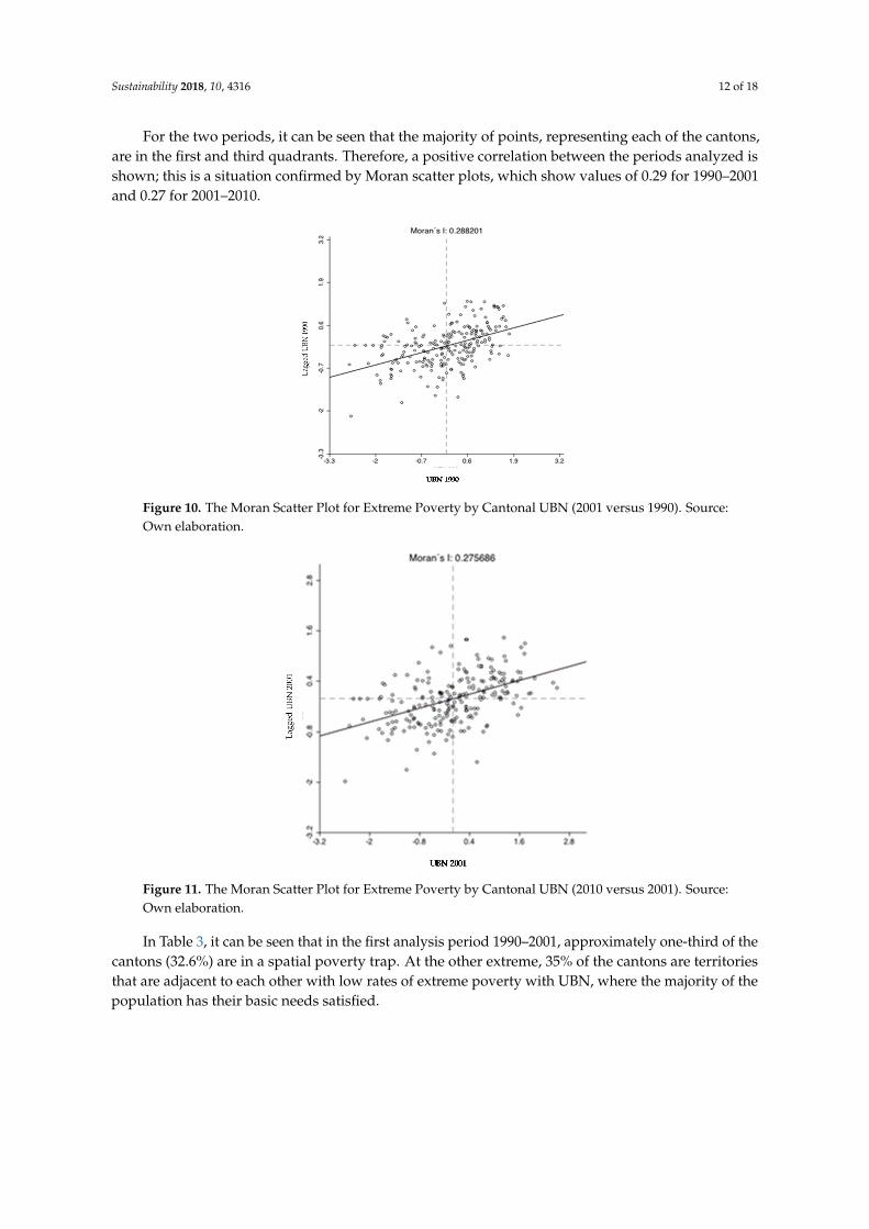
For the two periods, it can be seen that the majority of points, representing each of the cantons, are in the first and third quadrants. Therefore, a positive correlation between the periods analyzed is shown; this is a situation confirmed by Moran scatter plots, which show values of 0.29 for 1990–2001 and 0.27 for 2001–2010.
Figure 10. The Moran Scatter Plot for Extreme Poverty by Cantonal UBN (2001 versus 1990). Source: Own elaboration.
Figure 8. Poverty clusters by municipalities in the year 2001. Source: Own elaboration.
Sustainability 2018, 10, x FOR PEER REVIEW 11 of 18
Figure 8. Poverty clusters by municipalities in the year 2001. Source: Own elaboration.
Figure 9. Poverty clusters by municipalities in the year 2010. Source: Own elaboration.
For the two periods, it can be seen that the majority of points, representing each of the cantons, are in the first and third quadrants. Therefore, a positive correlation between the periods analyzed is shown; this is a situation confirmed by Moran scatter plots, which show values of 0.29 for 1990–2001 and 0.27 for 2001–2010.
Figure 10. The Moran Scatter Plot for Extreme Poverty by Cantonal UBN (2001 versus 1990). Source: Own elaboration.
Figure 9. Poverty clusters by municipalities in the year 2010. Source: Own elaboration.
Sustainability 2018, 10, 4316 12 of 18
For the two periods, it can be seen that the majority of points, representing each of the cantons,are in the first and third quadrants. Therefore, a positive correlation between the periods analyzed isshown; this is a situation confirmed by Moran scatter plots, which show values of 0.29 for 1990–2001and 0.27 for 2001–2010.
Sustainability 2018, 10, x FOR PEER REVIEW 11 of 18
Figure 8. Poverty clusters by municipalities in the year 2001. Source: Own elaboration.
Figure 9. Poverty clusters by municipalities in the year 2010. Source: Own elaboration.
For the two periods, it can be seen that the majority of points, representing each of the cantons, are in the first and third quadrants. Therefore, a positive correlation between the periods analyzed is shown; this is a situation confirmed by Moran scatter plots, which show values of 0.29 for 1990–2001 and 0.27 for 2001–2010.
Figure 10. The Moran Scatter Plot for Extreme Poverty by Cantonal UBN (2001 versus 1990). Source: Own elaboration.
Figure 10. The Moran Scatter Plot for Extreme Poverty by Cantonal UBN (2001 versus 1990). Source:Own elaboration.Sustainability 2018, 10, x FOR PEER REVIEW 12 of 18
Figure 11. The Moran Scatter Plot for Extreme Poverty by Cantonal UBN (2010 versus 2001). Source: Own elaboration.
In Table 3, it can be seen that in the first analysis period 1990–2001, approximately one-third of the cantons (32.6%) are in a spatial poverty trap. At the other extreme, 35% of the cantons are territories that are adjacent to each other with low rates of extreme poverty with UBN, where the majority of the population has their basic needs satisfied.
Table 3. Spatial lag of the UBN
Spatial lag of the UBN (1990)
LH 32
(14.3%)
HH 73
(32.6%) Spatial lag of the UBN (2001)
LH 38
(17%)
HH 75
(33.5%) LL 79
(35.3%)
HL 40
(17.9%)
LL 84
(37.5%)
HL 27
(12%) UBN (2001) UBN (2010)
Source: Own elaboration. HH: High–High, HL: High–Low, LH: Low–High, LL: Low–Low.
Figure 12 shows that for the year 2001, the number of cantons that were in a spatial poverty trap was 73, which was distributed as follows:
• Forty-two were located mainly on the Ecuadorian Coast in the provinces of Esmeraldas (four), Manabí (17), Los Ríos (seven), Guayas (12), Santa Elena (one), and El Oro (one).
• Twenty-one were located in the Ecuadorian Sierra in the provinces of Chimborazo (two), Cotopaxi (two), Cañar (three), Azuay (three), and Loja (11).
• Seven were located in the Ecuadorian East, corresponding to the provinces of Sucumbíos (two), Orellana (one), Morona Santiago (one), and Zamora Chinchipe (three). The remaining three correspond to the non-delimited zones, which were already mentioned.
In the second period (2001–2010), 75 cantons were in a poverty trap; that is, 33.5% of the cantons remained in a situation in which the UBN of a significant number of their inhabitants continued to be unmet or unsatisfied; while in 84 cantons, their population, due to structural factors or the attention (investment) by the state, preserved living conditions superior to the national averages by relating them spatially and temporally (Graph 8). In 2010, of the 75 cantons that were in a spatial poverty trap (Figure 13):
Figure 11. The Moran Scatter Plot for Extreme Poverty by Cantonal UBN (2010 versus 2001). Source:Own elaboration.
In Table 3, it can be seen that in the first analysis period 1990–2001, approximately one-third of thecantons (32.6%) are in a spatial poverty trap. At the other extreme, 35% of the cantons are territoriesthat are adjacent to each other with low rates of extreme poverty with UBN, where the majority of thepopulation has their basic needs satisfied.

Sustainability 2018, 10, 4316 13 of 18
Table 3. Spatial lag of the UBN
Spatial lag ofthe UBN (1990)
LH32(14.3%) HH73(32.6%) Spatial lag ofthe UBN (2001)
LH38(17%) HH75(33.5%)
LL79(35.3%) HL40(17.9%) LL84(37.5%) HL27(12%)
UBN (2001) UBN (2010)
Source: Own elaboration. HH: High–High, HL: High–Low, LH: Low–High, LL: Low–Low.
Figure 12 shows that for the year 2001, the number of cantons that were in a spatial poverty trapwas 73, which was distributed as follows:
• Forty-two were located mainly on the Ecuadorian Coast in the provinces of Esmeraldas (four),Manabí (17), Los Ríos (seven), Guayas (12), Santa Elena (one), and El Oro (one).
• Twenty-one were located in the Ecuadorian Sierra in the provinces of Chimborazo (two),Cotopaxi (two), Cañar (three), Azuay (three), and Loja (11).
• Seven were located in the Ecuadorian East, corresponding to the provinces of Sucumbíos (two),Orellana (one), Morona Santiago (one), and Zamora Chinchipe (three). The remaining threecorrespond to the non-delimited zones, which were already mentioned.
In the second period (2001–2010), 75 cantons were in a poverty trap; that is, 33.5% of the cantonsremained in a situation in which the UBN of a significant number of their inhabitants continued to beunmet or unsatisfied; while in 84 cantons, their population, due to structural factors or the attention(investment) by the state, preserved living conditions superior to the national averages by relatingthem spatially and temporally (Graph 8). In 2010, of the 75 cantons that were in a spatial poverty trap(Figure 13):
• Thirty-nine were located mainly on the Ecuadorian Coast in the provinces of Esmeraldas (four),Manabí (17), Los Ríos (five), Guayas (11), and Santa Elena (two).
• Twenty-five were located in the Ecuadorian Sierra in the provinces of Chimborazo (four),Cotopaxi (three), Bolívar (one), Cañar (two), Azuay (three), and Loja (12).
• Nine were located in the Ecuadorian East, corresponding to the provinces of Sucumbíos (one),Orellana (one), Pastaza (one), Morona Santiago (four), and Zamora Chinchipe (two); while theremaining two cantons corresponded to the non-delimited zones.
Sustainability 2018, 10, x FOR PEER REVIEW 13 of 18
• Thirty-nine were located mainly on the Ecuadorian Coast in the provinces of Esmeraldas (four), Manabí (17), Los Ríos (five), Guayas (11), and Santa Elena (two).
• Twenty-five were located in the Ecuadorian Sierra in the provinces of Chimborazo (four), Cotopaxi (three), Bolívar (one), Cañar (two), Azuay (three), and Loja (12).
• Nine were located in the Ecuadorian East, corresponding to the provinces of Sucumbíos (one), Orellana (one), Pastaza (one), Morona Santiago (four), and Zamora Chinchipe (two); while the remaining two cantons corresponded to the non-delimited zones.
Figure 12. Location of municipalities in a poverty trap condition in 2001.
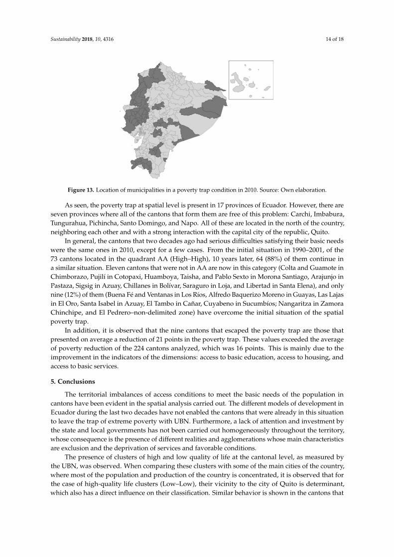
Figure 13. Location of municipalities in a poverty trap condition in 2010. Source: Own elaboration.
As seen, the poverty trap at spatial level is present in 17 provinces of Ecuador. However, there are seven provinces where all of the cantons that form them are free of this problem: Carchi, Imbabura, Tungurahua, Pichincha, Santo Domingo, and Napo. All of these are located in the north of the country, neighboring each other and with a strong interaction with the capital city of the republic, Quito.
In general, the cantons that two decades ago had serious difficulties satisfying their basic needs were the same ones in 2010, except for a few cases. From the initial situation in 1990–2001, of the 73 cantons located in the quadrant AA (High–High), 10 years later, 64 (88%) of them continue in a similar situation. Eleven cantons that were not in AA are now in this category (Colta and Guamote in Chimborazo, Pujilí in Cotopaxi, Huamboya, Taisha, and Pablo Sexto in Morona Santiago, Arajunjo in Pastaza, Sigsig in Azuay, Chillanes in Bolívar, Saraguro in Loja, and Libertad in Santa Elena), and only nine (12%) of them (Buena Fé and Ventanas in Los Ríos, Alfredo Baquerizo Moreno in Guayas, Las Lajas in El Oro, Santa Isabel in Azuay, El Tambo in Cañar, Cuyabeno in Sucumbíos; Nangaritza
Figure 12. Location of municipalities in a poverty trap condition in 2001.
Sustainability 2018, 10, 4316 14 of 18
Sustainability 2018, 10, x FOR PEER REVIEW 13 of 18
• Thirty-nine were located mainly on the Ecuadorian Coast in the provinces of Esmeraldas (four), Manabí (17), Los Ríos (five), Guayas (11), and Santa Elena (two).
• Twenty-five were located in the Ecuadorian Sierra in the provinces of Chimborazo (four), Cotopaxi (three), Bolívar (one), Cañar (two), Azuay (three), and Loja (12).
• Nine were located in the Ecuadorian East, corresponding to the provinces of Sucumbíos (one), Orellana (one), Pastaza (one), Morona Santiago (four), and Zamora Chinchipe (two); while the remaining two cantons corresponded to the non-delimited zones.
Figure 12. Location of municipalities in a poverty trap condition in 2001.
Figure 13. Location of municipalities in a poverty trap condition in 2010. Source: Own elaboration.
As seen, the poverty trap at spatial level is present in 17 provinces of Ecuador. However, there are seven provinces where all of the cantons that form them are free of this problem: Carchi, Imbabura, Tungurahua, Pichincha, Santo Domingo, and Napo. All of these are located in the north of the country, neighboring each other and with a strong interaction with the capital city of the republic, Quito.
In general, the cantons that two decades ago had serious difficulties satisfying their basic needs were the same ones in 2010, except for a few cases. From the initial situation in 1990–2001, of the 73 cantons located in the quadrant AA (High–High), 10 years later, 64 (88%) of them continue in a similar situation. Eleven cantons that were not in AA are now in this category (Colta and Guamote in Chimborazo, Pujilí in Cotopaxi, Huamboya, Taisha, and Pablo Sexto in Morona Santiago, Arajunjo in Pastaza, Sigsig in Azuay, Chillanes in Bolívar, Saraguro in Loja, and Libertad in Santa Elena), and only nine (12%) of them (Buena Fé and Ventanas in Los Ríos, Alfredo Baquerizo Moreno in Guayas, Las Lajas in El Oro, Santa Isabel in Azuay, El Tambo in Cañar, Cuyabeno in Sucumbíos; Nangaritza
Figure 13. Location of municipalities in a poverty trap condition in 2010. Source: Own elaboration.
As seen, the poverty trap at spatial level is present in 17 provinces of Ecuador. However, there areseven provinces where all of the cantons that form them are free of this problem: Carchi, Imbabura,Tungurahua, Pichincha, Santo Domingo, and Napo. All of these are located in the north of the country,neighboring each other and with a strong interaction with the capital city of the republic, Quito.
In general, the cantons that two decades ago had serious difficulties satisfying their basic needswere the same ones in 2010, except for a few cases. From the initial situation in 1990–2001, of the73 cantons located in the quadrant AA (High–High), 10 years later, 64 (88%) of them continue ina similar situation. Eleven cantons that were not in AA are now in this category (Colta and Guamote inChimborazo, Pujilí in Cotopaxi, Huamboya, Taisha, and Pablo Sexto in Morona Santiago, Arajunjo inPastaza, Sigsig in Azuay, Chillanes in Bolívar, Saraguro in Loja, and Libertad in Santa Elena), and onlynine (12%) of them (Buena Fé and Ventanas in Los Ríos, Alfredo Baquerizo Moreno in Guayas, Las Lajasin El Oro, Santa Isabel in Azuay, El Tambo in Cañar, Cuyabeno in Sucumbíos; Nangaritza in ZamoraChinchipe, and El Pedrero–non-delimited zone) have overcome the initial situation of the spatialpoverty trap.
In addition, it is observed that the nine cantons that escaped the poverty trap are those thatpresented on average a reduction of 21 points in the poverty trap. These values exceeded the averageof poverty reduction of the 224 cantons analyzed, which was 16 points. This is mainly due to theimprovement in the indicators of the dimensions: access to basic education, access to housing, andaccess to basic services.
5. Conclusions
The territorial imbalances of access conditions to meet the basic needs of the population incantons have been evident in the spatial analysis carried out. The different models of development inEcuador during the last two decades have not enabled the cantons that were already in this situationto leave the trap of extreme poverty with UBN. Furthermore, a lack of attention and investment bythe state and local governments has not been carried out homogeneously throughout the territory,whose consequence is the presence of different realities and agglomerations whose main characteristicsare exclusion and the deprivation of services and favorable conditions.
The presence of clusters of high and low quality of life at the cantonal level, as measured bythe UBN, was observed. When comparing these clusters with some of the main cities of the country,where most of the population and production of the country is concentrated, it is observed that forthe case of high-quality life clusters (Low–Low), their vicinity to the city of Quito is determinant,which also has a direct influence on their classification. Similar behavior is shown in the cantons that
Sustainability 2018, 10, 4316 15 of 18
are adjacent to the cities of Cuenca and Machala. However, the same is not true for the cantons thathave a very close proximity to the city of Guayaquil on the Ecuadorian coast.
The importance of these types of studies for Ecuador lies in the need for the geographicidentification of clusters, whereby profiles, situations, and categorizations of territories that sharecommon characteristics can be obtained. In the same way, hubs of development or of economic andsocial backwardness of regions can be obtained, as well as degrees of influence or geographic patternsthat have brought changes in their condition over time. The results of this study can be used to betterfocus resources, projects, and programs aimed at improving the living conditions of the populationof the affected municipalities; this is because currently, public policies must consider the territorialcomponent to set the guidelines and strategies by the state.
The limitation of this research is the unavailability of disaggregated updated data at cantonal level,so the most recent information used corresponds to the 2010 census. However, the results obtained willallow in the future identifying the evolution of poverty traps over three decades with the applicationof the census planned for 2020.
Author Contributions: All authors contributed equally to this work. All authors wrote, reviewed and commentedon the manuscript. All authors have read and approved the final manuscript.
Funding: This research received no external funding.
Conflicts of Interest: The authors declare no conflict of interest.
References
1. Chiriboga, M.; Wallis, B. Diagnóstico de la pobreza rural en Ecuador y respuestas de política pública. In Grupode Trabajo Sobre Pobreza Rural; Centro Latinoamericano para el Desarrollo Rural: Santiago, Chile, 2010.
2. García-Vélez, D. La pobreza en Ecuador a través del índice P de Amartya Sen: 2006–2014. Economía 2015, 40,91–115.
3. Ruíz, L.; Sánchez, N. La literatura ecuatoriana sobre pobreza urbana. In Pobreza Urbana en el Ecuador-Bibliografía Nacional; CIUDAD-UNICEF: Quito, Ecuador, 1994.
4. Barreiros, L.; Kouwenaar, A.; Teekebz, R.; Vos, R. La distribución de los Niveles de vida en Ecuador Ecuador;Teoría y Diseño de Políticas para la Satisfacción de las Necesidades Básicas (No. E51 B271); Institute of SocialStudies: Santiago, Ecuador, 1987.
5. Cobos, G. Desarrollo local y pobreza: Desigualdades socioterritoriales. In La Economía Política de la Pobreza;Cimadamore, A., Ed.; CLACSO: Buenos Aires, Argentina, 2008.
6. Skoufias, E.; Lopez-Acevedo, G. Latin America-Determinants of Regional Welfare Disparities within Latin AmericanCountries: Country Case Studies (No. 3051); Synthesis: Hertfordshire, UK, 2009.
7. IBRD-World Bank. Ecuador Poverty Assessment; Report No. 27061-EC; The World Bank: Washington, DC,USA, 2004.
8. Boisier, S. Origen, Evolución y Situación Actual de Las Políticas Territoriales en América Latina en Los Siglos XX yXXI; Planificación, Prospectiva y Gestión Pública, Reflexiones Para la Agenda de Desarrollo; Sn: Santiago,Chile, 2014.
9. Scott, L.M.; Janikas, M.V. Spatial statistics in ArcGIS. In Handbook of Applied Spatial Analysis—Software Tools,Methods and Applications; Fischer, M.M., Getis, A., Eds.; Springer: Berlin, Heidelberg, 2010; pp. 27–41.
10. Béland, E.; Escobar, G. Caracterización Socioeconómica de diez Parroquias de la Provincia de Tungurahua, Ecuador;Los Indicadores de Pobreza por Consumo: Santiago, Chile, 2011.
11. Burgos, S. Evolución de la Pobreza y Desigualdad de Ingresos 2006–2012. Notas Técnicas deInvestigación Económica N0. 5, 2013. Available online: http://www.sciencespo.fr/opalc/sites/sciencespo.fr.opalc/files/Evoluci%C3%B3n-de-pobreza-y-desigualdad-de-ingresos-2006-2012_SBD_def.pdf (accessed on14 September 2018).
12. SIISE. Sistema de Indicadores Sociales del Ecuador. Desigualdad y Pobreza, 2018. Available online: http://www.siise.gob.ec/siiseweb/siiseweb.html?sistema=1# (accessed on 14 September 2018).
13. Ministerio de Coordinación de Desarrollo Social. Mapa de Desigualdad y Pobreza en Ecuador, Quito-Ecuador:Editorial Aries; Ministerio de Coordinación de Desarrollo Social: Quito, Ecuador, 2012.
Sustainability 2018, 10, 4316 16 of 18
14. ECLAC. Ecuador: Mapa de Necesidades Básicas Insatisfechas. Naciones Unidas, Cepal (División de Estadística yProyecciones); PNUD-RLA/86/004; ECLAC: Santiago, Chile, 1989.
15. CONADE. Mapa de la Pobreza Consolidado; CONADE: Quito, Ecuador, 1993.16. INEC. Compendio de las Necesidad Básicas Insatisfechas de la Población Ecuatoriana; Instituto Nacional de
Estadísticas y Censos: Guayaquil, Ecuador, 1995.17. Larrea, C.; Andrade, J.; Brborich, W.; Jarrín, D.; Reed, C. Geografía de la pobreza en el Ecuador. In Geografía
de la Pobreza en el Ecuador; United Nations Development Programme—Facultad Latinoamericana de CienciasSociales: Quito, Ecuador, 1996.
18. Larrea, C. Desarrollo Social y Gestión Municipal en el Ecuador: Jerarquización y Tipología; ODEPLAN: Quito,Ecuador, 1999.
19. SIISE—STMCDS. Mapa de Pobreza y Desigualdad en Ecuador; INNFA: Guayaquil, Ecuador; Editorial Aries:Quito, Ecuador, 1996.
20. SIISE—STMCDS. Mapa de Pobreza y Desigualdad en Ecuador; INNFA: Guayaquil, Ecuador; Editorial Aries:Quito, Ecuador, 2010.
21. SENPLADES. Atlas de Las Desigualdades Socio Económicas en el Ecuador; TRAMA Ediciones: Quito,Ecuador, 2013.
22. Banerjee, A.; Duflo, E. Poor Economics: A Radical Rethinking of the Way to Fight Global Poverty; Public Affairs,Perseus Books: New York, NY, USA, 2011.
23. Barrientos, J.; Gòmez, W.; Rhenals, R. Crecimiento, distribución y pobreza en América Latina: Un ejerciciode panel, 1990–2005. Perf. Coyunt. Econ. 2008, 11, 15–50.
24. Carter, M.R.; Barrett, C.B. The economics of poverty traps and persistent poverty: An asset-based approach.J. Dev. Stud. 2006, 42, 178–199. [CrossRef]
25. Islam, T.M.; Minier, J.; Ziliak, J.P. On persistent poverty in a rich country. Southern Econ. J. 2015, 81, 653–678.[CrossRef]
26. Mayer-Foulkes, D. Globalization and the Human Development Trap (No. 2007/64); Research Paper; UNU-WIDER,United Nations University (UNU): Tokyo, Japan, 2007.
27. Burdín, G.; Ferrando, M.; Leites, M.; Salas, G. Trampas de Pobreza: Concepto y Medición Nueva Evidencia Sobre laDinámica del Ingreso en Uruguay; Fondo Concursable Carlos Filgueira: Montevideo, Uruguay, 2009; p. 195.
28. Arim, R.; Brum, M.; Dean, A.; Leites, M.; Salas, G. Movilidad de ingreso y trampas de pobreza: Nuevaevidencia para los países del Cono Sur. Estud. Econ. 2013, 28, 3–38.
29. Zhang, H. The poverty trap of education: Education–poverty connections in Western China. Int. J. Educ. Dev.2014, 38, 47–58. [CrossRef]
30. Dutta, S. Identifying Single or Multiple Poverty Trap: An Application to Indian Household Panel Data.Soc. Indic. Res. 2015, 120, 157–179. [CrossRef]
31. Giesbert, L.; Schindler, K. Assets, shocks, and poverty traps in rural Mozambique. World Dev. 2012, 40,1594–1609. [CrossRef]
32. Galvis, L.A.; Meisel, A. Persistencia de Las Desigualdades Regionales en Colombia: Un Análisis Espacial;Documentos de Trabajo Sobre Economía Regional, 120; Centro de Estudios Económicos Regionales–CERBanco de La República: Bogotá, Colombia, 2010.
33. Argüello, C.R.; Zambrano, A. ¿Existe una trampa de pobreza en el sector rural en Colombia? Rev. Desarro. Soc.2006, 58, 85–113. [CrossRef]
34. Agostini, C.A.; Brown, P.H.; Góngora, D.P. Spatial distribution of poverty in Chile. Estud. Econ. 2008, 35,79–110.
35. Pereira, M.; Soloaga, I. Trampas de pobreza y desigualdad en México 1990–2000–2010; Serie Documentos deTrabajo. Documento, 134; RIMISP-Centro Latinoamericano para el Desarrollo Rural: Santiago, Chile, 2014.
36. Thomas, A.C.; Gaspart, F. Does Poverty Trap Rural Malagasy Households? World Dev. 2015, 67, 490–505.[CrossRef]
37. Tavares, J.M.; Junior, S.D.S.P. “Corredores Da Pobreza” E “Ilhas De Prosperidade”: Uma análise espacial emultidimensional dos níveis de desenvolvimento na região sul do Brasil. Anál. Rev. Adm. PUCRS 2010, 21,51–62.
38. Yúnez, A.; Arellano, J.; Méndez, J. Cambios en el bienestar de 1990 a 2005: Un estudio espacial para México.Estud. Econ. 2010, 25, 363–406.
Sustainability 2018, 10, 4316 17 of 18
39. Risso Brandon, F.; Pasquier-Doumer, L. Aspiration Failure: A Poverty Trap for Indigenous Children in Peru?(No. 123456789/12016); Dauphine University: Paris, France, 2013.
40. Rowntree, B.S. Poverty: A Study of Town Life; Macmillan and Company Ltd.: London, UK; New York, NY,USA, 1901.
41. Townsend, P. The meaning of poverty. Br. J. Sociol. 1962, 13, 210–227. [CrossRef]42. Runciman, W.G. Relative Deprivation & Social Justice: Study Attitudes Social Inequality in 20th Century England;
Routledge and Kegan Paul: London, UK, 1966.43. Atkinson, A.B. On the measurement of inequality. J. Econ. Theory 1970, 2, 244–263. [CrossRef]44. Sen, A. An Ordinal Approach to Measurement. Econometrica 1976, 44, 219–231. [CrossRef]45. Chaudhuri, S.; Ravallion, M. How well do static indicators identify the chronically poor? J. Public Econ. 1994,
53, 367–394. [CrossRef]46. Kaztman, R. Virtudes y Limitaciones de los Mapas Censales de Carencias Críticas; Revista de la Cepal,
58 (LC/G.1916-P); CEPAL: Santiago, Chile, 1996.47. Feres, J.C.; Mancero, X. El Método de las Necesidades Básicas Insatisfechas (NBI) y sus Aplicaciones en América
Latina; Naciones Unidas Comisión Económica para América Latina y el Caribe (CEPAL): Santiago, Chile, 2001.48. Sen, A. Inequality Reexamined; Oxford University Press: Oxford, UK, 1992.49. Bourguignon, F.; Chakravarty, S.R. The measurement of multidimensional poverty. J. Econ. Inequal. 2003, 1,
25–49. [CrossRef]50. Alkire, S.; Foster, J. Recuento y Medición Multidimensional de la Pobreza; OPHI Working Paper Series; OPHI:
Oxford, UK, 2007; Volume 7, pp. 1–45.51. Domínguez Domínguez, J.; Martín Caraballo, A.M. Medición de la pobreza: Una revisión de los principales
indicadores. Rev. Métod. Cuantitativos Econ. Empres. 2006, 2, 27–66.52. Grupo de Río. Compendio de Mejores Prácticas en la Medición de la Pobreza; Grupo de Río: Santiago, Chile,
2007; Available online: http://www.eclac.cl/deype/publicaciones/sinsigla/xml/9/34409/rio_group_compendium_es.pdf (accessed on 1 September 2018).
53. Núñez Velázquez, J.J. Estado actual y nuevas aproximaciones a la medición de la pobreza. Estud. Econ. Apl.2009, 27, 325–344.
54. Feres, J.C.; Mancero, X. Enfoques Para la Medición de la Pobreza: Breve Revisión de la Literatura; Serie EstudiosEstadísticos y Prospectivos CEPAL, (4); Naciones Unidas Comisión Económica para América Latina y elCaribe (CEPAL): Santiago, Chile, 2001.
55. Silva Arias, A. Una primera revisión de las medidas de pobreza. Rev. Fac. Cienc. Econ. Investig. Reflex. 2005,13, 53–71.
56. Martínez Bernal, B.L. Planteamientos sobre la pobreza: Una aproximación conceptual. Apunt. CENES 2015,34, 15–40. [CrossRef]
57. Tukey, J.W. Exploratory Data Analysis; Addison-Wesley: Boston, MA, USA, 1977.58. Yrigoyen, C.C. Análisis estadístico de datos geográficos en geomarketing: El programa GeoDa.
Distrib. Consum. 2006, 2, 34–45.59. Anselin, L. Spatial Data Analysis with SpaceStatTM and ArcView, Workbook, 3rd ed.; Department of Agricultural
and Consumer Economics; University of Illinois: Chicago, IL, USA; Urbana, IL, USA, 1999.60. Moran, P.A. Notes on continuous stochastic phenomena. Biometrika 1950, 37, 17–23. [CrossRef] [PubMed]61. Celemín, J.P. Autocorrelación espacial e indicadores locales de asociación espacial: Importancia, estructura y
aplicación. Rev. Univ. Geogr. 2009, 18, 11–31.62. Bohórquez, I.A.; Ceballos, E.V. Algunos conceptos de la econometría espacial y el análisis exploratorio de
datos espaciales. Ecos Econ. 2008, 12, 2–25.63. Pearson, K. Mathematical contributions to the theory of evolution. III. Regression, heredity, and panmixia.
Philosophical Transactions of the Royal Society of London. Ser. A Contain. Pap. Math. Phys. Charact. 1986,187, 253–318.
64. Goodchild, M. Spatial autocorrelation. In Encyclopedia of Geographic Information Science; Karen, K., Ed.; SAGE:Thousand Oaks, CA, USA, 2008; pp. 397–398.
65. Dale, M.R.; Fortin, M.J. Spatial Analysis: A Guide for Ecologists; Cambridge University Press: Cambridge,UK, 2014.
66. Rivero, M.S. Análisis espacial de datos y turismo: Nuevas técnicas para el análisis turístico. Una aplicaciónal caso extremeño. Rev. Estud. Empres. 2008, 2, 48–66.
Sustainability 2018, 10, 4316 18 of 18
67. Geary, R.C. The contiguity ratio and statistical mapping. Incorp. Stat. 1954, 5, 115–146. [CrossRef]68. Getis, A.; Ord, J.K. The analysis of spatial association by use of distance statistics. Geogr. Anal. 1992, 24,
189–206. [CrossRef]69. Anselin, L. Spatial econometrics in RSUE: Retrospect and prospect. Reg. Sci. Urban Econ. 2007, 37, 450–456.
[CrossRef]70. Díaz, A.M.; Torres, F.J.S. Geografía de Los Cultivos Ilícitos y Conflicto Armado en Colombia; Universidad de los
Andes, Facultad de Economía, CEDE: Bogota, Colombia, 2004.71. Buzai, G. Los Sistemas de Información Geográfica y sus métodos de análisis en el continuo resolución-
integración. In Memorias X Conferencia Iberoamericana de Sistemas de Información Geográfica (X CONFIBSIG);Universidad de Puerto Rico: Río Piedras, Puerto Rico, 2005.
72. Anselin, L. Local indicators of spatial association—LISA. Geogr. Anal. 1995, 27, 93–115. [CrossRef]73. Ord, J.K.; Getis, A. Local spatial autocorrelation statistics: Distributional issues and an application.
Geogr. Anal. 1995, 27, 286–306. [CrossRef]74. Unwin, A. Exploratory spatial analysis and local statistics. Comput. Stat. 1996, 11, 387–400.75. Sánchez-Peña, L.L. Alcances y límites de los métodos de análisis espacial para el estudio de la pobreza
urbana. Pap. Poblac. 2012, 18, 147–180.76. Yue, W.; Zhang, Y.; Ye, X.; Cheng, Y.; Leipnik, M. Dynamics of multi-scale intra-provincial regional inequality
in Zhejiang, China. Sustainability 2014, 6, 5763–5784. [CrossRef]77. Zhang, J.; Deng, W. Multiscale Spatio-Temporal Dynamics of Economic Development in an Interprovincial
Boundary Region: Junction Area of Tibetan Plateau, Hengduan Mountain, Yungui Plateau and SichuanBasin, Southwestern China Case. Sustainability 2016, 8, 215. [CrossRef]
78. Pérez, G.J. Dimensión Espacial de la Pobreza en Colombia; Ensayos sobre Política Económica, No. 54; Banco dela Republica de Colombia: Cartagena, Colombia, 2005; pp. 234–293.
79. Muñetón, G.; Vanegas, J.G. Análisis espacial de la pobreza en Antioquia, Colombia. Equidad Desarro. 2014,21, 29–47. [CrossRef]
80. Tian, Y.; Wang, Z.; Zhao, J.; Jiang, X.; Guo, R. A Geographical Analysis of the Poverty Causes in China’sContiguous Destitute Areas. Sustainability 2018, 10, 1895. [CrossRef]
81. Jurado, A.; Pérez, J. Análisis de las diferencias espaciales de las tasas de pobreza. In XV Encuentro de EconomíaPública: Políticas Públicas y Migración; S.n.: Salamanca, España, 2008; p. 21.
82. Bolívar Espinoza, G.A.; Caloca Osorio, Ó.R. Distribución espacial de la pobreza Distrito Federal de México1990-2040. Polis-Rev. Latinoam. 2011, 10, 19–53. [CrossRef]
83. Wu, J.X.; He, L.Y. Urban–rural gap and poverty traps in China: A prefecture level analysis. Appl. Econ. 2018,50, 3300–3314. [CrossRef]
84. Serrano, A. Análisis de condiciones de vida, el mercado laboral y los medios de producción e inversiónpública. In Cuaderno de Trabajo Secretaria Nacional de Planificación y Desarrollo; SENPLADES: Quito, Ecuador,2013; pp. 1–248.
85. Haining, R.P. Spatial Data Analysis: Theory and Practice; Cambridge University Press: Cambridge, UK, 2003.86. Anselin, L. What is special about spatial data? Alternative perspectives on spatial data analysis. In
Spatial Statistics, Past, Present and Future; Griffith, D.A., Ed.; Institute of Mathematical Geography (IMAGE):Ann Arbor, MI, USA, 1989; pp. 66–77.
87. Anselin, L. Spatial Data Analysis with GIS: An Introduction to Application in the Social Sciences; National Centerfor Geographic Information and Analysis, University of California: Santa Barbara, CA, USA, 1992; pp. 10–92.
88. Tobler, W.R. Cellular geography. In Philosophy in geography; Springer: Dordrecht, The Netherlands, 1979;pp. 379–386.
89. Cliff, A.D.; Ord, J.K. Spatial Autocorrelation; Pion: London, UK, 1973; Volume 5.90. Upton, G.; Fingleton, B. Spatial Data Analysis by Example; Volume 1: Point Pattern and Quantitative Data;
John Wiley & Sons Ltd.: Chichester, UK, 1985.
© 2018 by the authors. Licensee MDPI, Basel, Switzerland. This article is an open accessarticle distributed under the terms and conditions of the Creative Commons Attribution(CC BY) license (http://creativecommons.org/licenses/by/4.0/).