Department of Agricultural and Resource EconomicsUniversity of California Davis

Poverty and Access to Infrastructure in Papua New Guinea

by

John Gibson and Scott Rozelle

Working Paper No. 02-008

February, 2002

Copyright @ 2000 John Gibson and Scott RozelleAll Rights Reserved. Readers May Make Verbatim Copies Of This Document For Non-Commercial Purposes By

Any Means, Provided That This Copyright Notice Appears On All Such Copies.

California Agricultural Experiment StationGiannini Foundation for Agricultural Economics

Poverty and Access to Infrastructure in Papua New Guinea

John Gibson†

University of Waikato

and

Scott RozelleUniversity of California, Davis

Abstract

In this paper, our overall goal is to understand how effective access to infrastructure is inreducing poverty in PNG. To meet this goal, we examine poverty in PNG, and seek to show therelationship between poverty and access to infrastructure and then identify the determinants ofpoverty. In our analysis, we test whether or not access to infrastructure is a significant factor in ahousehold's poverty status. Finally, we want to understand what policies will be effective inovercoming poverty in PNG. Our results show that poverty in PNG is primarily rural and isassociated with those in communities with poor access to services, markets, and transportation.Our simulations illustrate that improving access to school leads to large declines in poverty.Increasing access to poverty for those that are currently most isolated would have a significanteffect in decreasing the severity of poverty.

JEL: I32, O15Keywords:; Poverty, Papua New Guinea

We are grateful for helpful discussions with Gaurav Datt, Alan deBrauw and William Scribney. This research wasoriginally part of a World Bank poverty assessment for Papua New Guinea, for which financial support from thegovernments of Australia (TF-032753), Japan (TF-029460), and New Zealand (TF-033936) is gratefullyacknowledged.

______________† Department of Economics, University of Waikato, Private Bag 3105, Hamilton, New Zealand.Fax: (64-7) 838-4331. E-mail: jkgibson@waikato.ac.nz.

1

Poverty and Access to Infrastructure in Papua New Guinea

When considering the role that infrastructure can play in poverty alleviation and the size of

investments by developing countries into infrastructure, it is somewhat surprising that so little work

has been done on such an important topic.1 Developing countries invest over $200 billion US

dollars per year into basic infrastructure, about 4 percent of their Gross Domestic Product (World

Bank, 1994). While there are many reasons for these investments, different arguments can be made

as to why basic infrastructure investments in a developing country would be effective in reducing

poverty (Lipton and Ravallion, 1995). One is that poor areas have the least access to infrastructure

and so will benefit the most from new investments. If infrastructure provides benefits to a nation's

people and previous investments have mostly been in nonpoor areas, then new projects should

provide most of the benefits for the poor. Another argument is that the poor are concentrated in

sectors of the economy in which rates of return to infrastructure are high (van de Walle, 1985).

The Papua New Guinea (PNG) economy provides a unique opportunity to study the effect

of access to infrastructure on poverty. Because of PNG's unique status as such a late developing

country (one in which vast parts of the country remained isolated from the rest of world until after

1950) and because of its mountainous and rugged terrain, the country suffers from a fragmented

system of transportation (World Bank, 1999).2 In cities and some better-off rural areas, residents

1 Although there is less understanding of the relationship between the level of investment in basic infrastructure andpoverty than other aspects of poverty allevation (e.g., migration or agriculture), economists have begun payingattention to the infrastructure linkages that bind rich and poor areas together and the impact of these on growth (forexample, Binswanger, Khandker, and Rosenzweig, 1993; World Bank, 1994; van de Walle and Nead, 1995; Fan,Hazell, and Thorat, 1999; Jacoby, 2000).

2 Indeed, PNG is a country that has one of the most fragmented highway networks and most difficult terrain in theworld. In a study on the benefits of rural roads in Nepal, Jacoby (2000) claims he has chosen an interesting place towork because of the extreme need for roads. The mean travel time in Nepal between the average household and thenearest marketing center is 2.8 hours. Arguably, however, PNG’s rural communities are even more isolated. Theaverage travel time to the nearest government station (which is the closest thing in PNG to a Nepali market town) ismore than 3 hours. The average travel time to the nearest road is 2.5 hours. Moreover, this geographic isolation isexacerbated by extreme social-ethnic heterogeneity. Within the confines of a nation with only 4 million people, thepopulation is home to 850 separate languages, one-seventh of the world’s total (Grimes, 1992).

2

have access to multiple modes of transportation--paved roads, airports, and water travel. In poorer

areas, however, a high proportion of PNG's rural residents live many hours from the nearest basic

social services. And, while recent investment in rural infrastructure has made PNG compare

favorably with other developing countries in terms of meters of roads per person and per square

kilometer, access to many social services is still poor mainly because the road system is poorly

maintained and frequently inaccessible during and after rains. In fact, in some areas the

deterioration of roads has reached such a serious level that it has pushed local rural residents to

demonstrate and even riot when national ministers visit.

In this paper, our overall goal is to understand how effective access to infrastructure is in

reducing poverty in PNG. To meet this goal, we pursue three objectives. First, we examine

poverty in PNG, and seek to show the relationship between poverty and access to infrastructure.

Next, we identify the determinants of poverty, most importantly testing whether or not access to

infrastructure, ceteris paribus, is a significant factor in a household's poverty status. Finally, we

want to understand what infrastructure-related policies will be effective in overcoming poverty in

PNG.

To meet these goals and objectives, the rest of the paper is organized as follows. In section

II, we first describe our study's data set and explain how we created our measures of poverty. In

the next section, we examine the contours of poverty and its relationship to the access that PNG

residents have to infrastructure. Section IV creates a model of the determinants of poverty and

presents result about the effect that access to infrastructure has on the poor. We simulate the

impact of various investment strategies on poverty. The final section concludes.

To narrow the scope of our analysis, we focus on rural poverty for two reasons. First, as we

will show, most of the poor in PNG live and work in rural areas, a characteristic common to most

3

Asian countries. Second, the main infrastructure problems in PNG are in the rural areas. Access to

services, markets and transportation, measured in travel time, are much better in cities.

II. Data and Measures of Poverty

Data used in this paper come from the Papua New Guinea Household Survey (PNGHS),

which is the first nation-wide survey of consumption and living standards in PNG. The survey

design and enumeration, which was overseen by the authors in 1995 and 1996, covered a random

sample of 1200 households, residing in 120 rural and urban Primary Sampling Units (PSUs).

Enumerators conducted interviews between January and December 1996. The survey team

selected PSUs from the enumeration areas of the 1990 Census, stratifying the sample by sector (the

National Capital District was separated from the rest of the country), by environmental conditions

(elevation and rainfall), and by the level of agricultural development.3 A set of household weights

were derived from the variation between the 1990 Census estimates of the size of each cluster and

the actual size found during the survey, and from the deviation of the actual number of households

surveyed in each cluster from the target number. The results reported below are estimated from the

1144 households that had complete information on their consumption, and take account of the

clustered, stratified and weighted nature of the sample.

The survey interviewed each household twice, with the start of the two-week consumption

recall period signaled by the first interview. This first interview also collected information on

education and literacy, occupations and employment (but not income levels), dwelling

characteristics and a limited range of questions on agricultural assets and inputs. The interview

team collected expenditure data on all food (36 categories) and other frequent expenses

3 This was established from an agricultural mapping project (Allen, Bourke and Hide, 1995).

4

(20 categories) during the recall period. The expenditure estimates include the imputed value of

own-production, net gifts received, and stock changes, so they should be a good measure of

consumption during the recall period.4 An annual recall covered 31 categories of infrequent

expenses. The survey also included an inventory of durable assets that we use to estimate the value

of the flow of services (from these assets), including rental services from owner-occupied

dwellings. In addition to the household interviews, a community questionnaire, conducted in both

urban and rural areas, collected information on prevailing prices, community facilities and

estimates of the time needed to reach the nearest public services. In asking about travel times, the

survey specifically asked documented the usual mode of travel, which in rural areas, was almost

exclusively by foot.5

Poverty lines were set for five regions of Papua New Guinea – the National Capital District

(NCD), the South Coast, the Highlands, the North Coast, and the Islands – using methods outlined

by Ravallion (1994).6 These poverty lines were based on baskets of locally consumed foods that

provide 2200 calories per day, using average prices obtained from the community questionnaires.

An allowance for non-f ood items was based on the typical value of non- food spending by households

whos e total expenditur e equals the cost of the food pover ty line, w here this displacement of r equir ed

food spending suggests that the included non-food ar e ess entials . The resulting poverty lines were

4 The monetary values for self-produced foods were the values used by respondents. Estimates of average expenditureare unchanged if these respondent-reported unit values are replaced by either cluster medians of the unit values orcluster averages of market prices (Gibson and Rozelle, 1998).

5 Travel time to the nearest road or alternative mode of transportation (e.g., plane or boat) in PNG is not subject to thesame problem of endogeneity raised by Jacoby (2000) in his study of access to markets by road travel. His concernabout the endogeneity of access to services arose from the idea that households with high plot values (his dependentvariable) might be able to afford to invest in better means of transportation, thus shortening travel time. In the case ofPNG, almost all travel time in rural areas is measured in terms of walking time on small dirt paths. No other mode oftransportation is available.

6 An "upper" poverty line and a "food" poverty line were also calculated and reported in World Bank (1999). Detailson the calculations of the poverty lines and the differences found when alternative poverty lines were used arediscussed there.

5

K779 per adult equivalent per year in the NCD, K496 in the Papuan/South Coast region, K390 in

the Highlands, K280 in the Momase/North Coast region and K424 in the New Guinea Islands

region, with a national average value of K400.7 Separate urban and rural poverty lines were not

calculated within regions because most regions had only one urban PSU included in the sample,

and there were no rural PSUs in the NCD region.

III. Poverty in PNG and the Nation's Infrastructure

Although PNG is classified as a lower-middle income country with an average annual per

capita income of US$890, the living standards of the vast majority of the population are akin to that

of low-income countries (World Bank, 1999). PNG scores poorly on most social indicators

compared to its income level. Infant mortality per 1000 live births is 61. Life expectancy at birth

is only 58 years. Only 22 percent of the population have access to adequate sanitation. More than

40 percent of children aged 0 to 5 years, and more than 50 percent of those in the poorest quartile,

are stunted (or have height for age scores less than -2.0). Although the nation is rich in natural

resources, its high Gini ratio is one of the highest in the world (48.4 for per capita expenditures).

The size of the gap between the rich and the poor suggests that many of its residents do not share

equally in the nation’s wealth (World Bank, 2001).

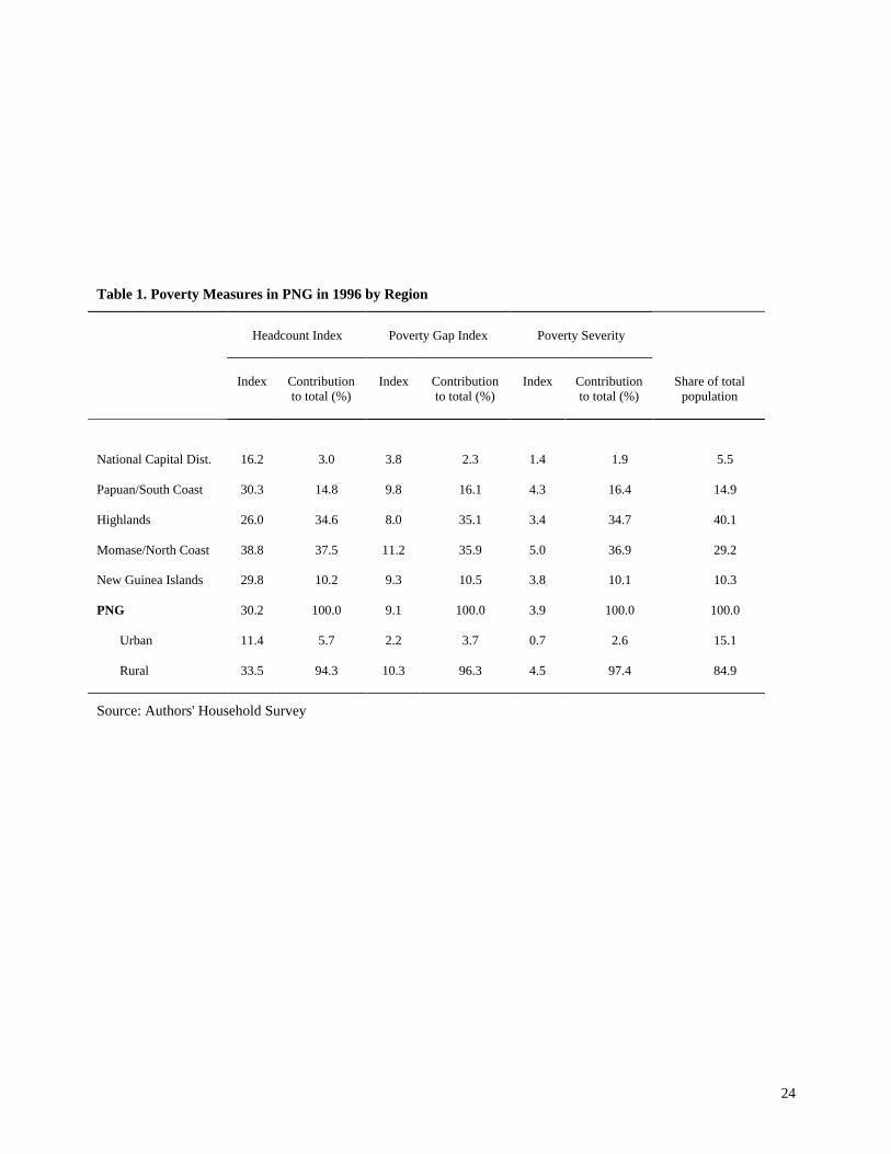
Poverty measures clearly illustrate the breadth and depth of poverty in PNG, especially in

the rural regions of the country (Table 1). Based on our estimated poverty line, 33.5 percent of

PNG’s rural population and 11.4 percent of the urban population live in households in which the

real value of consumption per adult equivalent is below the poverty line (rows 7 and 8). Overall (

7 The adult-equivalence scale counts children aged 0-6 years as 0.5 adults and all others as 1.0, and is based onestimates of child costs, made using the Engel and Rothbarth methods outlined by Deaton and Muellbauer (1986), and

6

since the rural population accounts for 85 percent of the nation's population—column 7), the

national headcount index of poverty is 30.2 percent (row 6). Using a more austere poverty line (the

food poverty line), slightly over one-sixth of the population have a total consumption valued at less

than the cost of the poverty line food basket, meaning that they could not even meet the basic

caloric requirement implied by the typical food consumption basket of the poor even if they spent

all their money on food. From these results it is clear that poverty in PNG is a rural problem. The

rural poor account for 94.3 percent of PNG’s poor.

While the headcount index indicates the proportion of the population with a standard of

living below the poverty line, the measure does not indicate how poor the poor are and does not

change if people below the poverty line become more or less poor. One indicator of the depth of

poverty, the poverty gap index, is constructed by measuring the income shortfall between the

standard of living of poor people and the poverty line. PNG’s gap index shows that the poor’s

income shortfall is equivalent to 9.1 percent of the value of the poverty line averaged over the

whole population (Table 1, columns 3 and 4).8 The poverty gap figures, like the head count

statistics, demonstrate rural nature of poverty. The poverty gap measure is nearly 5 times higher

for rural (10.3) than urban (2.2), and the rural poor account for an even larger share of the total

poverty gap (96.3 percent) than they do for the headcount index.

The poverty severity index is a distributionally sensitive poverty measure that takes into

account the distribution of consumption of those falling below the poverty line.9 This index (3.9

on a comparison of the dietary requirements of adults and children of various age groups. Details are provided byGibson and Rozelle (1998).8 The aggregate shortfall from the poverty line can also be calculated in monetary terms by multiplying the PG indexby the value of the poverty line and by the population size (4.3 million adult equivalents). This calculation shows thatit would require perfectly targeted (and costless) tranfers.

9 The hea dc ount index, the pove rty gap index, and the pover ty se ve rity index ca n all be e stima te d using the same genera l equation,through c hoice of values for a par ame te r ( Foste r, Gr ee r a nd Thor bec ke , 1984 – here af ter FGT) . The e qua tion is:

7

nation-wide) also shows that poverty is even deeper in rural areas of PNG (4.5) than in urban areas

(0.7--Table 1, columns 5 and 6). In other words, the extent by which the average consumption of

poor households in rural areas falls below the poverty line is significantly higher than that of poor

households in urban areas. Even more than the headcount or poverty gap index, the rural poor

contribute 97 percent of the poverty severity index.

Regional Patterns of Poverty

Finding out where poor people live is one of the most basic pieces of information for an

antipoverty program. Ideally, a household survey should be able to help in placing targeted

interventions. However, the diversity of environments in Papua New Guinea makes this an

impossible task for a survey of any feasible size. Even the more limited goal of estimating poverty

rates by province would require a very much larger household survey than the one conducted in

1996. Instead, the poverty comparisons presented here are for the four major geographical regions

of the country -- the Papuan/South Coast; the Highlands; Momase/North Coast; and the New

Guinea Islands. The map in appendix A illustrates the location of these areas.

The incidence and extent of poverty vary significantly across PNG's major regions (Table 1,

rows 1 to 5). Poverty is lowest in the NCD and highest in the Momase/North Coast region (column

1 and 2). Only about 16.2 percent of the population of the NCD falls below the poverty line.

Nearly 39 percent of the population in the Momase/North Coast region falls below the poverty line

and its share of national poverty is 37.5 percent. The other three regions (Papuan/South Coast,

Highlands, and New Guinea Islands) have poverty rates that are clustered slightly below the

P = 1

n

g

zj=1

qj�

��

�

↵√ wher e the pove rty line is z, the value of expe nditure pe r c apita f or the jth person's house hold is xj a nd the

pove rty gap for individual j is gj = z - xj. Total popula tion siz e is n a nd q is the number of poor people (those where xj < z). W henpa ra meter α is set to z er o, P0 is simply the he adcount inde x. When α is set e qua l to one, P1 is the pove rty gap inde x, and w he n α is setequa l to two, P2 is the pove rty severity inde x

8

national average, ranging from 26.0 percent to 30.3 percent. While the headcount of poverty is

higher in the Momase/North Coast region, the large population share in the Highlands (40.1

percent) means that the Highland's contribution to poverty is also high (34.6 percent—column 7).

The poverty gap and the poverty severity measures also are highest in the Momase/North Coast and

the Highland Regions.

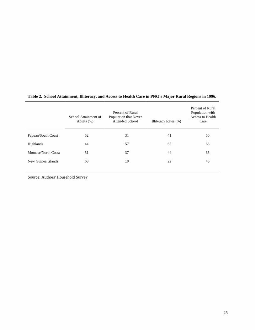
The poverty in PNG regions is closely correlated with the several important measures of

each region’s human capital, one of the most important indicators of PNG’s long term development

prospects. Educational attainment is lowest and the proportion of people who never attended

school is highest in the Highlands and the Momase/North Coast region (Table 2, columns 1 and 2).

Illiteracy rates are also highest in the two regions (column 3). Moreover, access to health services

is poorest in these regions (column 4). Although not as bad as the Highland and Momase/North

Coast, the record of education and health is not good in the Papuan/South Coast region and the

New Guinea Islands and relatively poorer than in the urban NCD.

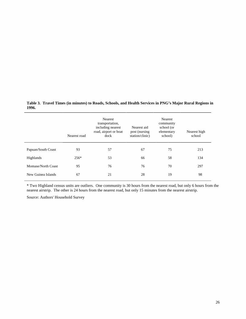
Given the remoteness and rugged terrain of PNG, poor access to roads may be one of the

proximate causes of poor record of the government in the provision of education, health and other

public goods. If roads are poor and travel time is high, the cost of attending school or seeking

health care may be prohibitively high. In fact, measures of the access to roads in PNG's four main

regions shows that road access in the two most poverty stricken regions (the Momase/North Coast

region and the Highlands) is the poorest (Table 3, column 1). In the Highlands, for example, rural

residents have to walk more than 4 hours to reach the nearest road. Travel times in the

Papuan/South Coast and the Momase/North Coast regions both exceed 90 minutes. While access

to any transportation mode (including boat docks and dirt airstrips) is better in the Highlands (than

9

the Momase or Papuan regions), individuals still have to walk about an hour, on average (column

2).

With road access so poor, access to health and educational services are poor. Access to aid

posts (PNG’s most basic health service centers) also is the poorest for the Highlands and the

Momase/North Coast region (although it is equally as poor for the Papua/South Coast

region—Table 3, column 3). Even to get access to the most basic health services, households in

these regions much walk from 66 to 76 minutes. Access to community schools is equally poor;

travel times in the poorest regions are all around one hour (column 4). Travel times to high schools

average more than 3 hours (column 5)

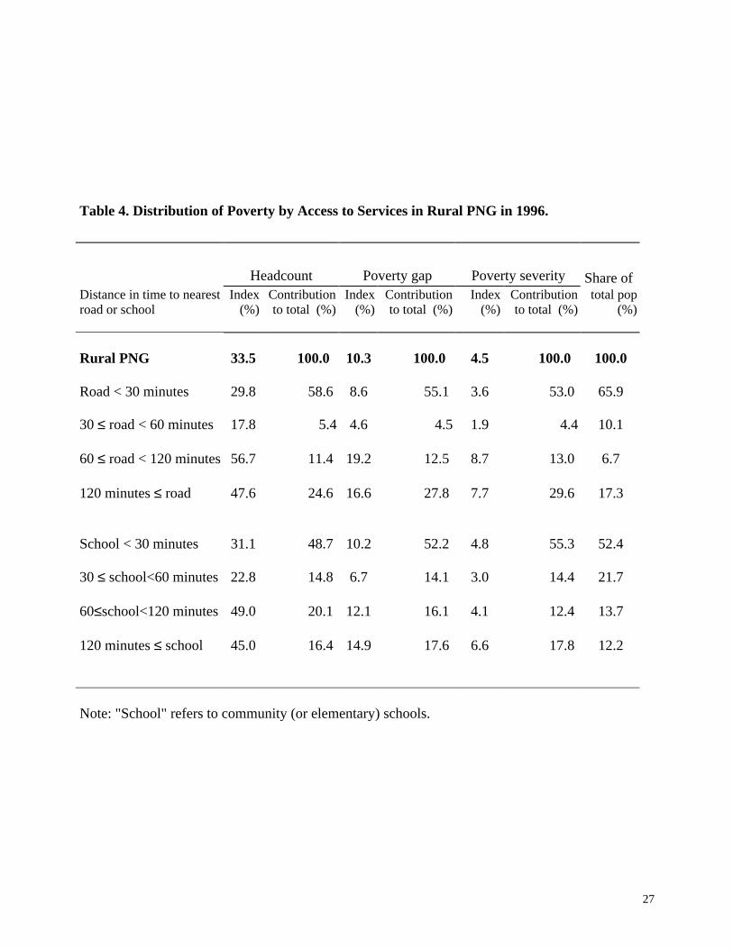
To illustrate an even closer linkage between poverty and rural infrastructure, Table 4

demonstrates the strong correlation between poverty, school attainment and access to roads.

According to the headcount measure of poverty (column 1), when households live more than 60

minutes from the nearest road (rows 4 and 5), the incidence of poverty more than doubles when

compared to those living less than 60 minutes from a road (rows 3 and 4). The same is true for

access to schooling (rows 6 to 9). Poverty headcount measures increase markedly when the nearest

school is more than 60 minutes away. The correlation between poverty measures and rural

infrastructure increases when the depth and severity of poverty indices are used (columns 3 and 5).

Consumption and Price Effects of Access to Roads

The effect of access to roads on poverty can most clearly be illustrated by the marked

differences in access to transportation infrastructure among income groups. The lowest

consumption quartile must travel over twice as long to gain access to the closest mode of transport

than the richest quartile. The poor travel 75 percent longer than the non-poor to the closest mode

of transportation and over three times longer to reach the closest road.

10

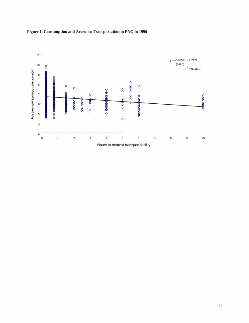
A simple regression of per capita consumption against travelling time to the nearest

transport facility demonstrates that consumption is negatively correlated with access to

transportation (Figure 1). A one-hour increase in travelling time to the nearest transport facility

reduces real consumption by 10 percent. This suggests that measures that improve the access of

rural communities to transport infrastructure could be an important aspect of poverty alleviation in

PNG.

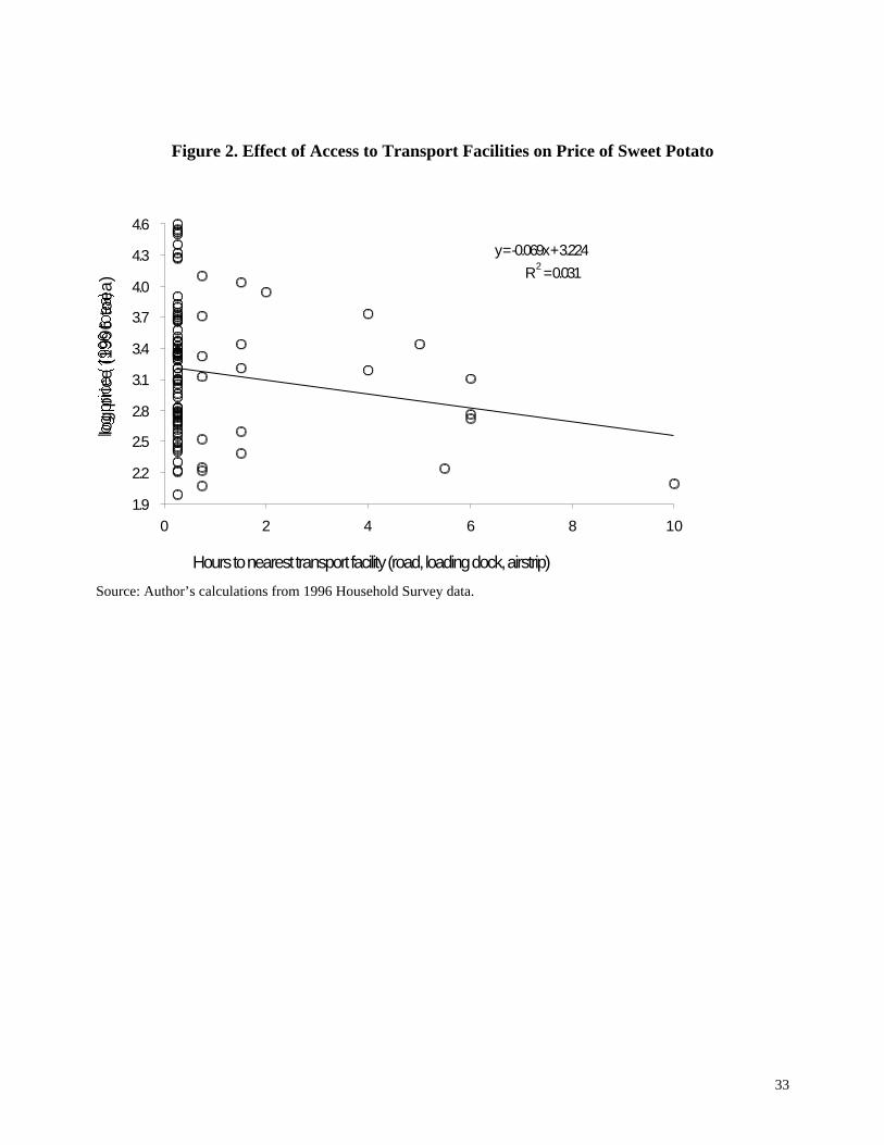
While there may be a number of effects of access to infrastructure that affect consumption

(for example, see Jacoby, 2000), our sample data clearly illustrate two. Access to a road affects the

price farmers receive for their crops and the prices that households must pay for their purchased

food (Figure 2). The relationship between the average price of sweet potato, calculated at a Census

Unit level, and the travelling time from the Census Unit to the nearest road or other transport

facility suggests that sweet potato prices are lower in communities that are further from roads and

other transport points.10 Specifically, the rate of price decline is around seven percent for each

extra hour to the nearest transport facility. This rate of price decline can also be interpreted as the

rate at which the net returns to marketing food and other crops produced by rural households

decline as infrastructure becomes less accessible.

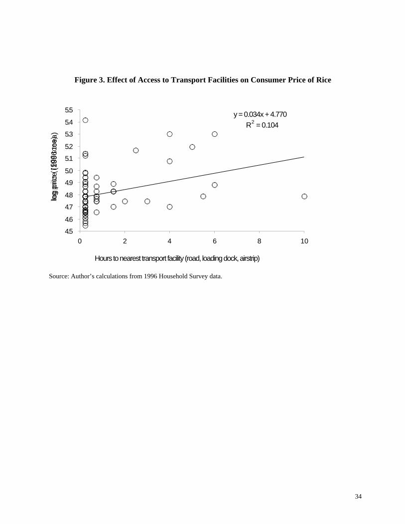
To provide additional evidence of the impact of transport facilities on food prices, the data

from the 1996 survey were used to calculate the average price (at the Census Unit level) on a one

kilogram packet of Trukai rice, one of the most widely available foods in trade stores across PNG

in 1996. Figure 3 demonstrates the relationship between the average price and the distance that

each Census Unit is from the nearest transport facility, such as a road, airstrip or boat docking

10 The sweet potato prices are shown using a logarithmic scale, so that the slope of the relationship can be directlyinterpreted as the percentage change in price when moving to a community that is an extra hour away from the nearesttransport point.

11

point. The slope of the regression suggests that each additional hour further away from transport

infrastructure raises the trade store price of rice by 3.4 percent (with a standard error of one percent,

making the regression coefficient highly statistically significant).11

Finally, roads and other transport infrastructure also give households better access to

markets that may help them engage in a wider range of income earning activities. This

diversification does not only increase income, it can help to stabilise the cash incomes of

households, and in this manner improve food security by increasing the reliability with which food

can be purchased to supplement own production. Some partial evidence for this point is presented

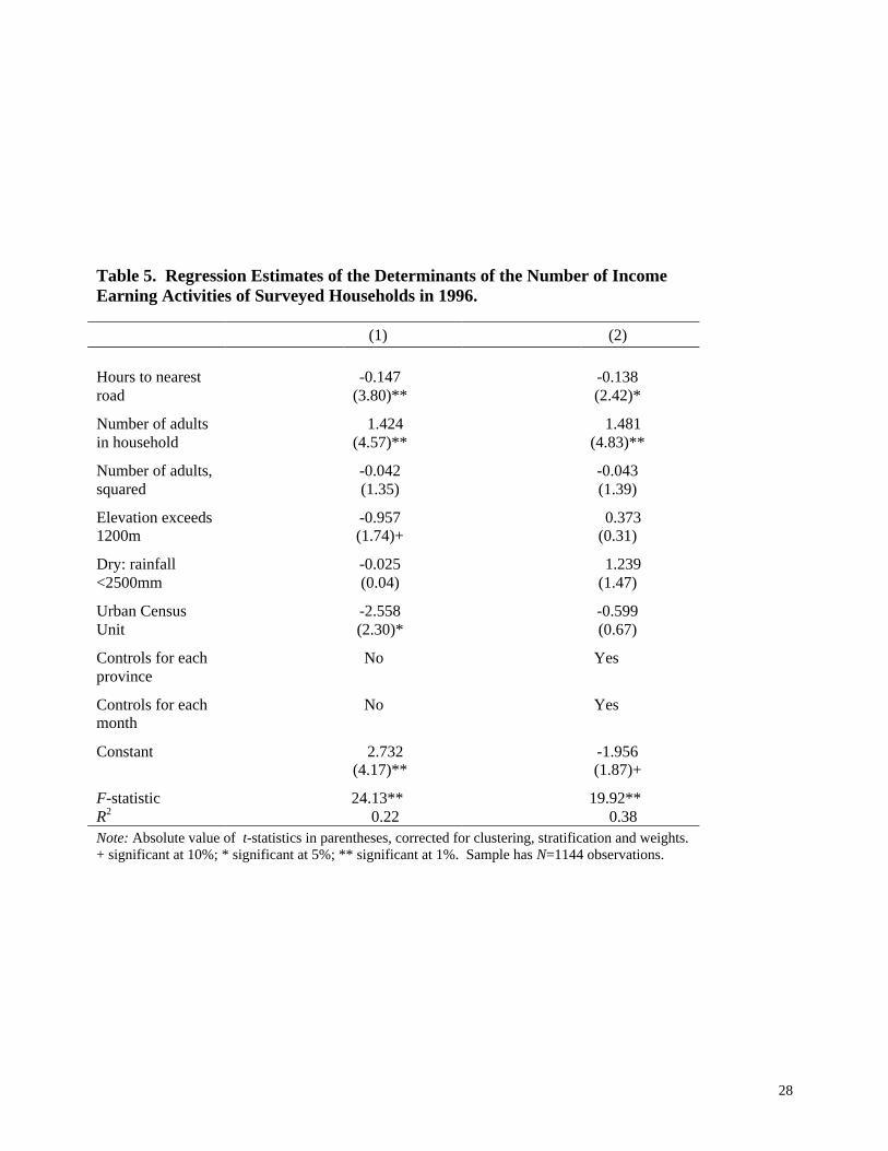
in Table 5, which contains the results of regression analyses of the number of income earning

activities engaged in by respondent households from the 1996 household survey.12 In this analysis,

each one-hour increase in travelling time to the nearest road appears to reduce the number of

income-earning activities by an average of 0.15, which is a 2.6 percent reduction in the number of

activities per extra hour to the road (column 1). This result is robust to the inclusion of provincial

and monthly dummies (column 2).

11 Of course, it is clear from the wide scatter of points on the graph that many things other than distance from roadsexplains the price of rice. Adding in control variables for each province (as a proxy for their distance from the ricemills and rice terminals) and for each month (as a proxy for the general price inflation occurring over the course of1996) raise the R2 to 0.48, so just under one half of the variation in rice prices is explained by these three factors. Mostimportantly, adding in these additional variables does not alter the basic relationship between transport access andprice, with each one hour increase in travelling time to the nearest transport facility estimated to cause a 2.8 percentincrease in the village-level price of rice (which is still statistically significant).

12 This is the household total of a question that is asked of each individual adult, in contrast to the 1990 Census whichasked about similar economic activities engaged in, but only at the household level. See Gibson, 2001 for a morecomplete and detailed argument.

12

IV. The Determinants of Poverty in PNG

While the profiles of poverty in PNG are a useful way of summarizing information on the

levels and location of poverty and on the characteristics of the poor, they are essentially cross-

tabulations and no matter how imaginative their uses (see, e.g., Grootaert, 1994), they are restricted

in the number of dimensions that can be varied at one time (e.g., poverty rates broken down by

region of residence and economic activity of the household head). To answer questions about the

effect of a particular variable, conditional on the many other potential determinants of poverty,

requires multivariate analysis. In particular, multivariate analysis may help show whether

geographical pockets of poverty exist just because people with poor endowments cluster together

(Ravallion, 1998).

A common approach to the multivariate analysis of poverty is to define a 0-1 variable; hi = 1

if the ith household’s per capita consumption expenditure, ci is less than the poverty line, z and

proceed with probit estimation:13

( )bxx iiih Φ==1Pr

w here Φ is the standar d cumulative nor mal, and X is the matrix of explanator y var iables. Us ually

inter est is not centr ed on the coeff icient vector b but on the ‘ pr obability der ivatives ’ which can be

obtained f r om b and s how the change in the ris k of pover ty as the explanator y var iables change.

A lthough this appr oach ignor es the depth and s ever ity of poverty, it might be jus tif ied by the

w ides pread concern of policy makers with the incidence of poverty. But unlike the usual case where

binary response models are used, the underlying variable that generates hi is fully observed, as can

be seen from the general equation for several common poverty measures for the ith household

(Foster, Greer and Thorbecke, 1984):

13

( )( )[ ] ,0 zc = P ii ?− 0,1max

where =0 gives the binary headcount measure of poverty, =1 gives the poverty gap index, and

=2 gives the squared poverty gap or poverty severity measure, which is sensitive to inequality

amongst the poor. Moreover, the parameters of interest – including the probability of the ith

household being poor – can be estimated more directly by regressing ci on xi – whilst making

weaker assumptions about the errors than are needed by probit models (Ravallion, 1998).

Rather than using poverty probits, the approach of this paper is to model the determinants of

consumption, using standard regression analysis, and then derive from the regression model

estimates of the various poverty measures following simulated changes in certain variables. More

specifically, the model is of (log) nominal consumption expenditure per adult equivalent, deflated

by region-specific poverty lines – a ratio known as the “welfare ratio” (Blackorby and Donaldson,

1987):

( ) iii uzc += bxln .

Because the poverty measures are homogeneous of degree zero, the results of the poverty

simulations should be the same if the ratio of the regional poverty lines was used as a spatial price

deflator and the regression was carried out using variables in real terms. Normalizing consumption

by the poverty line implies that ( ) 0ln <zci for poor households and the probability of the ith

household’s (log) welfare ratio being less than zero can be derived from the estimated parameter

vector b̂ and the standard error of the regression, ˆ :

( )( ) ( )( )ˆˆ0ˆlnprob bx ii zc −Φ=< .14

13 Examples include Bardhan (1984), Gaiha (1988) and Grootaert (1997). Gibson (1998) also uses this approach, forPNG urban poverty in the mid-1980s.14 One complication with this procedure is that to get an estimate of the standard error of the regression when the datacome do not come from a simple random survey, it may be necessary to use a pseudo-maximum likelihood estimator(see Skinner, Holt and Smith, 1989, pp. 80-83). The reason is that the usual regression estimator for clustered, stratified

14

A weighted average of the household probabilities of being poor gives the predicted

incidence of poverty, where the weights are the household sampling weights in terms of person-

numbers. This same approach can be extended to the simulated poverty gap and poverty severity

measures, when the integrals are solved in terms of the estimated log consumption model (Datt,

1998).

Model Specification

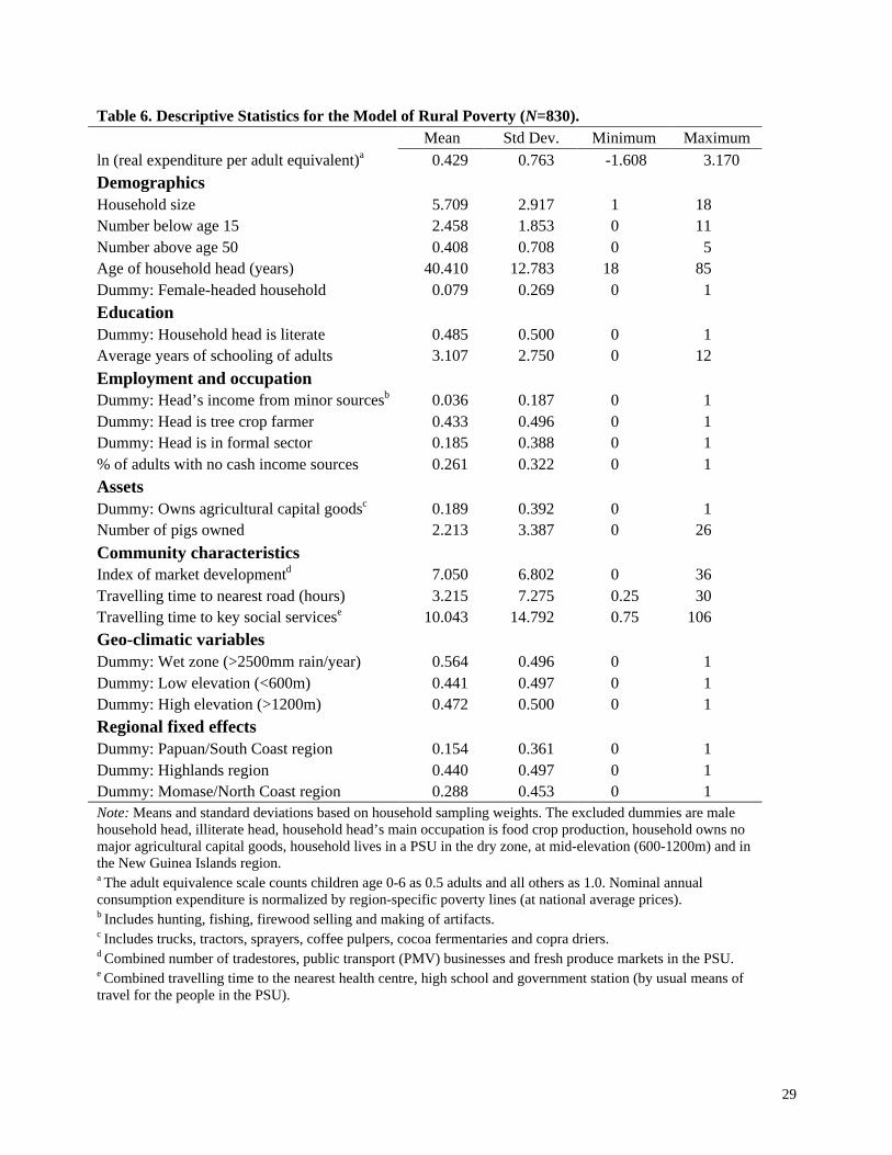
A wide range of variables measuring the potential determinants of rural poverty are available

from the survey and these are described under the following seven headings: demographics,

education, employment and occupations, assets, community characteristics, geo-climatic

characteristics, and regional fixed effects. Variables that directly contribute to the construction of

the dependent variable were ruled out as regressors because of the spurious relationships that may

be obtained. In particular, estimates of the value or possession of household durable goods and

dwelling characteristics are not included among the set of explanatory variables because the

imputed value of the use of durable goods and dwellings is already included as a component of

consumption.

Demographics: A linear and quadratic term in household size, the number of children (below

age 15) and number of elderly (above age 50) household members, plus linear and quadratic terms

in the age of the household head and a binary variable for female-headed households are included.

The welfare interpretations of some of the demographic variables is unclear because, for example,

the effect of household size may just be due to the excluded effects of scale economies in

and weighted survey data makes no assumptions about normality of the disturbances, and strictly speaking there is no σin such a model. The pseudo-maximum likelihood estimator relies on the stronger assumption of normality ofdisturbances in the population. This estimator can be implemented using the svyintreg command in Stata, and we aregrateful to William Scribney for advice on this issue.

15

consumption within households (Lanjouw and Ravallion, 1995), although attention has been paid

to the differing costs of children and adults.

Education: the household average of completed school years for those household members

over the age of 15 and a binary variable for whether the household head is literate are used.

Although correlated, something is gained by specifying these two variables separately. Literacy is a

basic functioning, which may help raise living standards even of those with little connection to the

market economy (e.g., semi-subsistence farmers reading food crop extension bulletins) while years

of schooling may matter both for human capital and screening reasons. Moreover, informal

teaching may allow literacy to improve even without raising average years of schooling, so it is

interesting to separate the two variables for policy simulations.

Employment and occupation: the household head’s main source of income was grouped into

four occupational classifications – formal sector, tree crop farmer, food crop farmer, and minor

occupations (hunting, fishing, firewood selling and making of artifacts). In addition, the proportion

of adults in each household who had no sources of cash income over the past 12 months was

included. This variable could be considered a measure of unemployment because the absence of a

labour market in most areas of PNG makes the usual definition of actively seeking work somewhat

inapplicable.

Assets: the survey did not collect information on land holdings, due to (i) the difficulty of

measuring this in a system of customary tenure with widely scattered plots, and (ii) the sensitivity

of the issue following a recent failed land registration drive. But data on the number of pigs, which

are the major type of livestock, are available and used. Also used is a dummy variable for whether

the household owned major agricultural capital goods (trucks, tractors, sprayers, coffee pulpers,

cocoa fermentaries and copra driers), where these goods – with the possible exception of trucks –

16

were not included in the list of household durables and so should not be spuriously related to

consumption expenditure.

Community characteristics: an index of market development, based on the combined number

of tradestores, public transport businesses and fresh produce markets located in the PSU, the

travelling time to the nearest road, and the combined travelling time to the nearest of each of three

key social services: high schools, health centres, and government stations. Although data on the

travelling time to lower level health (aid post) and education (community school) facilities are

available, the quality of these appears more variable than for the higher level services (but was not

measured by the survey); users sometimes appear to travel past the lower level services to reach the

higher level services of more consistent quality – making travelling time a more reliable measure of

access to public services for the higher level services. The index of market development is designed

to capture the notion that missing markets prevent households from gaining from specialisation,

thereby reducing living standards (e.g., minimising involvement in cash cropping because of

concerns about food market failures).

Geo-climatic characteristics: consumption and several of the household and community

characteristics are likely to be affected by various agroecological factors that impact the

productivity of land. Failure to control for this omission of relevant variables will give biased

results. For example, consumption and ownership of agricultural capital goods are both likely

lower in areas of poor agricultural potential, leading to a spurious positive effect if there is no

measure of agricultural potential in the model. The variables used are rainfall (a binary variable for

wet regions where annual rainfall exceeds 2500mm) and elevation (binary variables for three

zones, <600m, 600-1200m, and >1200m) which affects climate and limits the range of crops that

can be grown.

17

Regional fixed effects: Even with the geo-climatic variables, there are likely to be spatial

effects whose omission biases the coefficients on the included variables. Therefore, a set of fixed

effects are included. Although it is possible that the relevant fixed effects are at the PSU level,

capturing any unobserved community-level determinants of living standards, the inclusion of a

PSU set of intercept dummies would make it impossible to identify any of the community level

variables. As a compromise, the fixed effects are defined at regional (n=4) level.

Since our interest is on rural poverty, we report only estimate models for the rural sector.

We also estimate separate rural models since we believe that it is likely that there is genuine

heterogeneity in the effect of the independent variables on the welfare ratio across sectors, a

hypothesis that we test. Table 6 contains descriptive statistics on the variables in the model for

rural sector.

Determinant of Poverty Results

Since our interest is on rural poverty, we report only the results for the model estimated on

rural households. However, a similar model has been estimated on urban households and tests with

a pooled sample suggest that the coefficients were not the same across urban and rural sectors

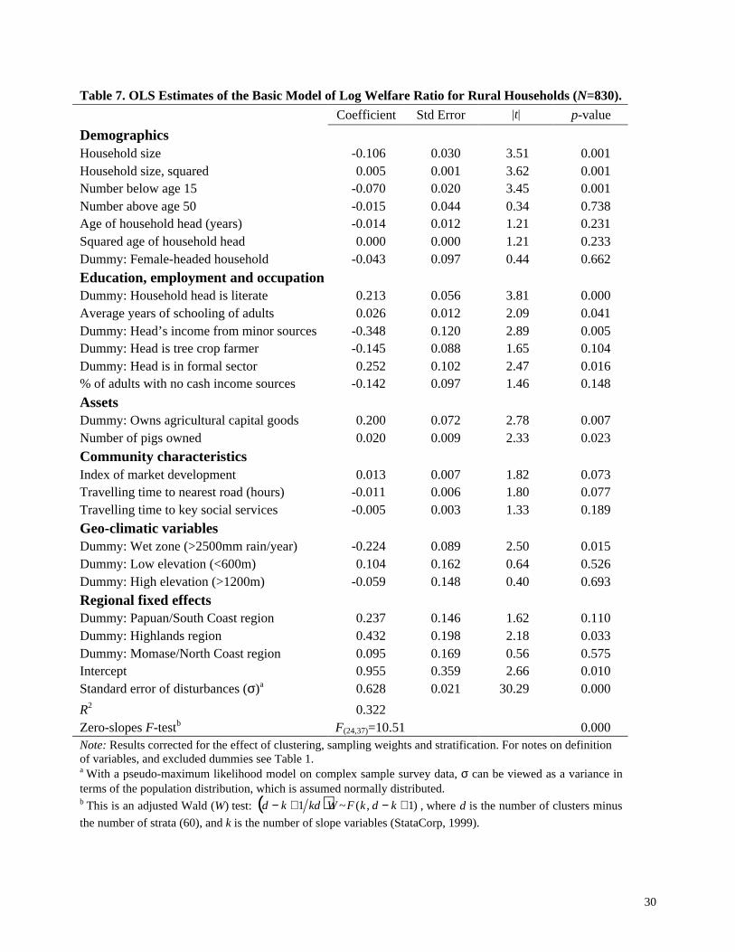
(World Bank, 1999). The results of the model for the rural sector are in Table 7.

In general, the model performed well. The goodness of fit measure, R2, was 0.32,

sufficiently high for models using cross sectional household data. In addition, many coefficients of

our control variables were of the expected sign and statistically significant. For example, the

results show that there are significant gains from both extra years of schooling and literacy of the

household head in rural areas. While participation by the household head in the formal sector does

affect consumption levels, the proportion of adults in the household without access to cash incomes

in the previous year does not emerge as a significant determinant of consumption. Finally, high

18

rainfall, but not elevation, emerges as a negative influence on consumption in rural areas while

regional fixed effects are also relevant.

Even after controlling for the demographic, educational, employment and environmental

factors, community characteristics appear to be relevant. Consumption in the rural sector rises with

market development. Moreover, as access to the nearest road falls (or travel time increases), the

rural welfare ratio falls. In other words, remoteness may matter to poverty not just because remote

areas tend to have people with poor endowments of human capital but because rural infrastructure

matters directly. Of course, part of the returns to education and occupation may be due to the ease

in which rural residents have access to these basic services and economic opportunities.

Concerned about differences among different types of households, Datt and Jolliffe (1999)

suggest that the marginal effects of household and community characteristics on consumption are

not constant across households and add interaction effects into their model to control for them.

Although every variable can potentially be interacted with every other variable, multicollinearity is

likely to result, with fragile coefficient estimates leading to potentially unreliable poverty

simulations. Therefore, Datt and Jolliffe restrict attention to just a few interactions, mainly between

schooling and other variables. After trying a large number of combinations, the presence of

interaction effects was not supported for the rural sector of PNG (p<0.43) and we must conclude

that in general, including the interaction terms did not change the coefficients on the community

characteristics. The only significant interaction effect that we could find was for lower returns to

education for female-headed households.15

19

Poverty Alleviation and Investments in Infrastructure

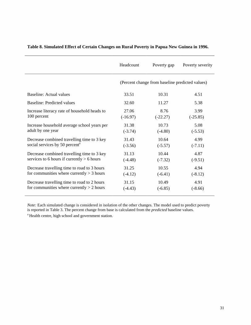
Table 8 reports the results of various poverty simulations done with the model in Table 7.

The beneficial effect of increasing literacy, schooling and access to social services and roads is

readily apparent from these simulations. The incidence of poverty would fall by 17 percent if all

household heads could be made literate (row 3). Although the incidence of poverty would fall by

only 3.74 percent, following a one year rise in average school years per adult, if the average

schooling in PNG was raised from the current level, 3 years, to a minimum of an elementary

(middle) school education, poverty could fall by more than 10 (20) percent (row 4). The depth and

severity of poverty measures would fall by a greater percentage since those in greatest poverty

currently have the least access to education (rows 3 and 4, columns 2 and 3). To the extent that

improved access to schooling in terms of travel times will assist in expanding education, PNG’s

poverty rates will be benefited by investments both in the education system itself and in the rural

infrastructure.

Increasing access to services will also have an independent effect on decreasing poverty.

The headcount index would fall by 3.56 percent if the travelling time to key social services could

be cut by 50 percent, with the greatest proportionate gain in the urban sector (row 5). If access to

the three key services were reduced by 50 percent for those who live more than 6 hours away from

them now, poverty could be reduced by 4.48 percent (row 6). Likewise, reducing the travelling

time to the nearest road would also be an effective anti-poverty strategy in the rural sector, with the

greatest gains arising from an approach targeted at the most remote households rather than on

making across-the-board cuts in travelling time to roads (rows 7 and 8). As in the case of

education, providing such services also targets the poorest of the poor, since in all cases, the depth

and severity indices fall faster than the headcount measures (rows 5 to 8, columns 2 and 3).

15 These results are not reported here for brevity but are in World Bank (1999).

20

V. Conclusions

Our results appear to support the argument that poor areas have the least access to

infrastructure and so people in those areas may benefit the most from new investments. Thus,

infrastructure spending, whether on new assets or maintenance of existing facilities, can provide a

form of targeted interventions that favors the poor. This is an especially relevant finding for PNG,

in part because the existing infrastructure is so poorly developed, and the returns to such projects

high. But more importantly, infrastructure spending may be one of the few feasible means for

policy interventions to reach the poor in PNG.

In many cases the results of poverty measurement and profiling exercises might be useful as

inputs into some system of directly targeting the poor, for example, by schemes based on cash

grants, food stamps or other selective subsidies. But in PNG there is little capacity to do this

because the vast majority of the poor are located in remote, rural areas and most have only limited

involvement in formal activities. While there is a value-added tax, it excludes transactions carried

out in informal markets. Since the poorest of the poor participate so little in the cash economy, this

means that there is little scope for targeting the poor by setting lower tax rates on basic

consumption items that are formally marketed, such as rice. Other approaches to targeting, such as

supporting cash crop prices, are also unlikely to be feasible because there is a history of these price

support schemes collapsing in PNG.

Papua New Guinea also is marked by an unusually low capacity of the government to

provide services to the poor, so other agencies such as churches fill the gap. For example, the

household survey shows that amongst the poorest quartile of the population, 42 percent of the

births taking place outside the home are in church-run health facilities (as compared to 13 percent

21

in the richest quartile). But it is a rather more difficult task for churches and NGOs to build major

infrastructure such as a road system, which remains an obvious role for the state.

22

References

Allen, B., Bourke, M., and Hide, R. 1995 The sus tainability of Papua N ew Guinea agr icultur alsystems : the conceptual background. Global Envir onmental Change, 5( 3): 297- 312.

Bardhan, P. K.1984. Land, labour and rural poverty: Essays in development economics. NewDelhi: Oxford University Press.

Binswanger, H., Khandker, S., and Rosenzweig, M.1993. How Infrastructure and FinancialInstitutions Affect Agricultural Output and Investment in India. Journal-of-Development-Economics, 41(2): 337-366.

Blackorby, C. and D. Donaldson. 1987. Welfare ratios and distributionally sensitive cost-benefitanalysis. Journal of Public Economics 34( ): 265-290.

Datt, Gaurav, and Dean Jolliffe. 1999. Determinants of poverty in Egypt. Food Consumption andNutrition Discussion Paper No. 75, International Food Policy Research Institute,WashingtonD.C.

Datt, Gaurav.1998. Simulating poverty measures from regression models of householdconsumption. International Food Policy Research Institute, Washington D.C. Photocopy.

Deaton, A., and Muellbauer, J. (1986) “On measuring child costs: with applications to poorcountries” Journal of Political Economy 96(4): 720-743.

Fan, Shenggen, Peter Hazell, and Sukhadeo Thorat. 1999. Linkages between government spending,growth, and poverty in rural India. Research Report 110. Washington, D.C.: InternationalFood Policy Research Institute.

Foster, J., Greer, J. and E. Thorbecke (1984) “A class of decomposable poverty measures”Econometrica 52(4): 761-765.

Gaiha, Raghav. 1988. On measuring the risk of rural poverty in India. In Rural poverty in SouthAsia, ed. T. N. Srinivasan and P. K. Bardhan, 219-261. Irvington, N.Y., U.S.A.: ColumbiaUniversity Press.

Gibson, John. 1998. Identifying the poor for efficient targeting: results for Papua New Guinea. NewZealand Economic Papers. 32(1): 1-18.

Grimes, Chris B. 1992. Hermans, -H.–E.-G.-M. Casparie,-A.-F.; Paelinck,-J.-H.-P., eds. Healthcare in Europe after 1992. Aldershot, U.K. and Sydney: Dartmouth; distributed in the U.S. byAshgate, Brookfield, Vt. pp. 205-09.

23

Grootaert, Christian.1997. Determinants of poverty in Côte d'Ivoire in the 1980s. Journal ofAfrican Economies 6 (2): 169-196.

Jacoby, Hanan G. 2000. Access to Markets and the Benefits of Rural Roads. The EconomicJournal. 110 (July): 713-737.

Lanjouw, P., and M. Ravallion. 1995. Poverty and household size. The Economic Journal 105(November): 1415-1434.

Lipton, M., and Ravallion, M. 1995. Poverty and Policy, in Jere Behrman and T.N. Srinivasan(eds) Handbook of Development Economics Volume 3 Amesterdam: North-Holland.

Ravallion, Martin. 1994. Poverty comparisons. Chur, Switzerland: Harwood AcademicPublishers.

Ravallion, Martin. 1998. “Poor areas” in A. Ullah and D. Giles (ed.) Handbook of AppliedEconomic Statistics Marcel Dekker, New York, pp. 63-91.

Skinner, C.J., Holt, D., and Smith, T.M.F. 1989. Analysis of Complex Surveys Wiley: New York.

van de Walle, Dominique. 1985. Population growth and poverty: Another look at the Indian timeseries data. Journal of Development Studies 21 (3): 429-439.

World Bank. 1994. “Governance: The World Bank’s Experience,” Working Paper, World Bank,Washington, DC.

World Bank. 1999. Papua New Guinea: Improving Governance and Performance. World Bank:Washington, DC.

World Bank. 2001. World Development Report, 2000. World Bank: Washington, DC.

24

Table 1. Poverty Measures in PNG in 1996 by Region

Headcount Index Poverty Gap Index Poverty Severity

Index Contributionto total (%)

Index Contributionto total (%)

Index Contributionto total (%)

Share of totalpopulation

National Capital Dist. 16.2 3.0 3.8 2.3 1.4 1.9 5.5

Papuan/South Coast 30.3 14.8 9.8 16.1 4.3 16.4 14.9

Highlands 26.0 34.6 8.0 35.1 3.4 34.7 40.1

Momase/North Coast 38.8 37.5 11.2 35.9 5.0 36.9 29.2

New Guinea Islands 29.8 10.2 9.3 10.5 3.8 10.1 10.3

PNG 30.2 100.0 9.1 100.0 3.9 100.0 100.0

Urban 11.4 5.7 2.2 3.7 0.7 2.6 15.1

Rural 33.5 94.3 10.3 96.3 4.5 97.4 84.9

Source: Authors' Household Survey

25

Table 2. School Attainment, Illiteracy, and Access to Health Care in PNG’s Major Rural Regions in 1996.

School Attainment ofAdults (%)

Percent of RuralPopulation that Never

Attended School Illiteracy Rates (%)

Percent of RuralPopulation withAccess to Health

Care

Papuan/South Coast 52 31 41 50

Highlands 44 57 65 63

Momase/North Coast 51 37 44 65

New Guinea Islands 68 18 22 46

Source: Authors' Household Survey

26

Table 3. Travel Times (in minutes) to Roads, Schools, and Health Services in PNG’s Major Rural Regions in1996.

Nearest road

Nearesttransportation,

including nearestroad, airport or boat

dock

Nearest aidpost (nursingstation/clinic)

Nearestcommunityschool (orelementary

school)Nearest high

school

Papuan/South Coast 93 57 67 75 213

Highlands 256* 53 66 58 134

Momase/North Coast 95 76 76 70 297

New Guinea Islands 67 21 28 19 98

* Two Highland census units are outliers. One community is 30 hours from the nearest road, but only 6 hours from thenearest airstrip. The other is 24 hours from the nearest road, but only 15 minutes from the nearest airstrip.

Source: Authors' Household Survey

27

Table 4. Distribution of Poverty by Access to Services in Rural PNG in 1996.

Headcount Poverty gap Poverty severity Share ofDistance in time to nearestroad or school

Index(%)

Contributionto total (%)

Index(%)

Contributionto total (%)

Index(%)

Contributionto total (%)

total pop(%)

Rural PNG 33.5 100.0 10.3 100.0 4.5 100.0 100.0

Road < 30 minutes 29.8 58.6 8.6 55.1 3.6 53.0 65.9

30 ≤ road < 60 minutes 17.8 5.4 4.6 4.5 1.9 4.4 10.1

60 ≤ road < 120 minutes 56.7 11.4 19.2 12.5 8.7 13.0 6.7

120 minutes ≤ road 47.6 24.6 16.6 27.8 7.7 29.6 17.3

School < 30 minutes 31.1 48.7 10.2 52.2 4.8 55.3 52.4

30 ≤ school<60 minutes 22.8 14.8 6.7 14.1 3.0 14.4 21.7

60≤school<120 minutes 49.0 20.1 12.1 16.1 4.1 12.4 13.7

120 minutes ≤ school 45.0 16.4 14.9 17.6 6.6 17.8 12.2

Note: "School" refers to community (or elementary) schools.

28

Table 5. Regression Estimates of the Determinants of the Number of IncomeEarning Activities of Surveyed Households in 1996.

(1) (2)

-0.147 -0.138Hours to nearestroad (3.80)** (2.42)*

1.424 1.481Number of adultsin household (4.57)** (4.83)**

-0.042 -0.043Number of adults,squared (1.35) (1.39)

-0.957 0.373Elevation exceeds1200m (1.74)+ (0.31)

-0.025 1.239Dry: rainfall<2500mm (0.04) (1.47)

-2.558 -0.599Urban CensusUnit (2.30)* (0.67)

Controls for eachprovince

No Yes

Controls for eachmonth

No Yes

Constant 2.732 -1.956(4.17)** (1.87)+

F-statistic 24.13** 19.92**R2 0.22 0.38Note: Absolute value of t-statistics in parentheses, corrected for clustering, stratification and weights.+ significant at 10%; * significant at 5%; ** significant at 1%. Sample has N=1144 observations.

29

Table 6. Descriptive Statistics for the Model of Rural Poverty (N=830).Mean Std Dev. Minimum Maximum

ln (real expenditure per adult equivalent)a 0.429 0.763 -1.608 3.170

DemographicsHousehold size 5.709 2.917 1 18Number below age 15 2.458 1.853 0 11Number above age 50 0.408 0.708 0 5Age of household head (years) 40.410 12.783 18 85Dummy: Female-headed household 0.079 0.269 0 1

EducationDummy: Household head is literate 0.485 0.500 0 1Average years of schooling of adults 3.107 2.750 0 12

Employment and occupationDummy: Head’s income from minor sourcesb 0.036 0.187 0 1Dummy: Head is tree crop farmer 0.433 0.496 0 1Dummy: Head is in formal sector 0.185 0.388 0 1% of adults with no cash income sources 0.261 0.322 0 1

AssetsDummy: Owns agricultural capital goodsc 0.189 0.392 0 1Number of pigs owned 2.213 3.387 0 26

Community characteristicsIndex of market developmentd 7.050 6.802 0 36Travelling time to nearest road (hours) 3.215 7.275 0.25 30Travelling time to key social servicese 10.043 14.792 0.75 106

Geo-climatic variablesDummy: Wet zone (>2500mm rain/year) 0.564 0.496 0 1Dummy: Low elevation (<600m) 0.441 0.497 0 1Dummy: High elevation (>1200m) 0.472 0.500 0 1

Regional fixed effectsDummy: Papuan/South Coast region 0.154 0.361 0 1Dummy: Highlands region 0.440 0.497 0 1Dummy: Momase/North Coast region 0.288 0.453 0 1Note: Means and standard deviations based on household sampling weights. The excluded dummies are malehousehold head, illiterate head, household head’s main occupation is food crop production, household owns nomajor agricultural capital goods, household lives in a PSU in the dry zone, at mid-elevation (600-1200m) and inthe New Guinea Islands region.a The adult equivalence scale counts children age 0-6 as 0.5 adults and all others as 1.0. Nominal annualconsumption expenditure is normalized by region-specific poverty lines (at national average prices).b Includes hunting, fishing, firewood selling and making of artifacts.c Includes trucks, tractors, sprayers, coffee pulpers, cocoa fermentaries and copra driers.d Combined number of tradestores, public transport (PMV) businesses and fresh produce markets in the PSU.e Combined travelling time to the nearest health centre, high school and government station (by usual means oftravel for the people in the PSU).

30

Table 7. OLS Estimates of the Basic Model of Log Welfare Ratio for Rural Households (N=830).

Coefficient Std Error |t| p-value

DemographicsHousehold size -0.106 0.030 3.51 0.001Household size, squared 0.005 0.001 3.62 0.001Number below age 15 -0.070 0.020 3.45 0.001Number above age 50 -0.015 0.044 0.34 0.738Age of household head (years) -0.014 0.012 1.21 0.231Squared age of household head 0.000 0.000 1.21 0.233Dummy: Female-headed household -0.043 0.097 0.44 0.662

Education, employment and occupationDummy: Household head is literate 0.213 0.056 3.81 0.000Average years of schooling of adults 0.026 0.012 2.09 0.041Dummy: Head’s income from minor sources -0.348 0.120 2.89 0.005Dummy: Head is tree crop farmer -0.145 0.088 1.65 0.104Dummy: Head is in formal sector 0.252 0.102 2.47 0.016% of adults with no cash income sources -0.142 0.097 1.46 0.148

AssetsDummy: Owns agricultural capital goods 0.200 0.072 2.78 0.007Number of pigs owned 0.020 0.009 2.33 0.023

Community characteristicsIndex of market development 0.013 0.007 1.82 0.073Travelling time to nearest road (hours) -0.011 0.006 1.80 0.077Travelling time to key social services -0.005 0.003 1.33 0.189

Geo-climatic variablesDummy: Wet zone (>2500mm rain/year) -0.224 0.089 2.50 0.015Dummy: Low elevation (<600m) 0.104 0.162 0.64 0.526Dummy: High elevation (>1200m) -0.059 0.148 0.40 0.693

Regional fixed effectsDummy: Papuan/South Coast region 0.237 0.146 1.62 0.110Dummy: Highlands region 0.432 0.198 2.18 0.033Dummy: Momase/North Coast region 0.095 0.169 0.56 0.575Intercept 0.955 0.359 2.66 0.010Standard error of disturbances (σ)a 0.628 0.021 30.29 0.000

R2 0.322Zero-slopes F-testb F(24,37)=10.51 0.000Note: Results corrected for the effect of clustering, sampling weights and stratification. For notes on definitionof variables, and excluded dummies see Table 1.a With a pseudo-maximum likelihood model on complex sample survey data, σ can be viewed as a variance interms of the population distribution, which is assumed normally distributed.b This is an adjusted Wald (W) test: ( ) )1,(~1 +−+− kdkFWkdkd , where d is the number of clusters minus

the number of strata (60), and k is the number of slope variables (StataCorp, 1999).

31

Table 8. Simulated Effect of Certain Changes on Rural Poverty in Papua New Guinea in 1996.

Headcount Poverty gap Poverty severity

(Percent change from baseline predicted values)

Baseline: Actual values 33.51 10.31 4.51

Baseline: Predicted values 32.60 11.27 5.38

Increase literacy rate of household heads to100 percent

27.06(-16.97)

8.76(-22.27)

3.99(-25.85)

Increase household average school years peradult by one year

31.38(-3.74)

10.73(-4.80)

5.08(-5.53)

Decrease combined travelling time to 3 keysocial services by 50 percenta

31.43(-3.56)

10.64(-5.57)

4.99(-7.11)

Decrease combined travelling time to 3 keyservices to 6 hours if currently > 6 hours

31.13(-4.48)

10.44(-7.32)

4.87(-9.51)

Decrease travelling time to road to 3 hoursfor communities where currently > 3 hours

31.25(-4.12)

10.55(-6.41)

4.94(-8.12)

Decrease travelling time to road to 2 hoursfor communities where currently > 2 hours

31.15(-4.43)

10.49(-6.85)

4.91(-8.66)

Note: Each simulated change is considered in isolation of the other changes. The model used to predict povertyis reported in Table 3. The percent change from base is calculated from the predicted baseline values.a Health centre, high school and government station.

32

Figure 1. Consumption and Access to Transportation in PNG in 1996

y = -0.1053x + 6.7172(t=6.6)

R2 = 0.0371

3

4

5

6

7

8

9

10

11

0 1 2 3 4 5 6 7 8 9 10

Hours to nearest transport facility

33

Figure 2. Effect of Access to Transport Facilities on Price of Sweet Potato

y = -0.069x + 3.224

R2 = 0.031

1.9

2.2

2.5

2.8

3.1

3.4

3.7

4.0

4.3

4.6

0 2 4 6 8 10

Hours to nearest transport facility (road, loading dock, airstrip)

log

pric

e (1

996

toea

)

Source: Author’s calculations from 1996 Household Survey data.

34

Figure 3. Effect of Access to Transport Facilities on Consumer Price of Rice

y = 0.034x + 4.770

R2 = 0.104

4.5

4.6

4.7

4.8

4.9

5.0

5.1

5.2

5.3

5.4

5.5

0 2 4 6 8 10

Hours to nearest transport facility (road, loading dock, airstrip)

log

pric

e (1

996

toea

)

Source: Author’s calculations from 1996 Household Survey data.