Poverty, adolescent well-being and outcomes later in life

Journal of International Development

J. Int. Dev. 22, 1162–1182 (2010)

Published online in Wiley Online Library

(wileyonlinelibrary.com) DOI: 10.1002/jid.1753

POVERTY, ADOLESCENT WELL-BEINGAND OUTCOMES LATER IN LIFE

MARK TOMLINSON* and ROBERT WALKER

University of Oxford, Oxford, UK

Abstract: This paper investigates the impact of various factors in childhood (such as

poverty, parental guidance, educational orientation, self-esteem and delinquent behaviour)

on outcomes later in life. Using data from the British Household Panel Survey which

incorporates a survey of children aged 11–15 years (also known as the British Youth Panel

(BYP)) the technique of Structural Equation Modelling is employed to show the relative

impact of these factors on educational attainment and employment status when the respon-

dents were in their late 20s. Copyright # 2010 John Wiley & Sons, Ltd.

Keywords: childhood; well-being; poverty; transmission of disadvantage; structural

equation models

1 INTRODUCTION

There is a large body of evidence from economically advanced countries, notably the

United States and Britain, documenting the transmission of disadvantage across

generations and a growing interest in this in the developing world. However, risking

over-simplification, different disciplines have tended to focus on different outcomes and

different routes of transmission. Educational outcomes have attracted much attention from

economists, social policy specialists, demographers and psychologists with economists

focussing on the role of income and psychologists on such mechanisms as parental

emotional investment and behaviour. Psychologists have also explored the impact of

poverty on physical, cognitive and emotional development; sociologists on social mobility,

teenage pregnancy, homelessness and crime; epidemiologists on drug abuse and physical

and mental health outcomes; and economists and social policy specialists on employment

as well as citizenship and civic participation.1

*Correspondence to: Mark Tomlinson, Department of Social Policy and Social Work, University of Oxford,32 Wellington Square, Oxford OX1 2ER, UK. E-mail: [email protected]

1See, for example, Istance et al., 1994; Craine, 1997; Dean, 1997; Hobcraft, 1998; Aber et al., 2000; Ermisch et al.,2001; Flouri and Buchanan, 2004; Lister, 2005; Stewart, 2005 and Fahmy, 2006.

Copyright # 2010 John Wiley & Sons, Ltd.

Poverty, adolescent well-being and outcomes 1163

There has been little cross-referencing between studies of transmission conducted in

advanced economies and those undertaken in a development context.2 Again this might

simply reflect different disciplinary perspectives but possibly also environmental

differences in that factors such as malnutrition, illiteracy and disease might be dominant

in the developing world while social and psychological variables could be more important

elsewhere. However, it is increasingly argued that differences are conceptually matters of

degree rather than kind and that there is a considerable scope for bidirectional learning

between the global South and North (White et al., 2005). Hence, using British data, this

paper exploits cross-disciplinary insights and explicitly demonstrates the power of

recent conceptual and technical advances to advance our understanding of the nature and

relative importance of the complex factors influencing the impact of poverty and childhood

well-being on outcomes in adulthood.

The focus is on the effects on early adulthood of poverty experienced by children when

they are aged between 11 and 15 years and the data derive from the British Household

Panel Study (BHPS). Data are currently available for 1991–2008 with, from 1994,

information derived from questionnaires completed by young people aged 11–15 years in

the panel households. This is known as the British Youth Panel (BYP). Children in the

Youth Panel become part of the main panel when they reach 16 years of age and are

continuously interviewed thereafter on an annual basis.

Using structural equation models (SEMs)—which link various factors and their causal

relations—the significance of the impact of poverty and well-being in adolescence will be

related with labour market and educational outcomes when the children reach their late

20s. In essence SEMs take observed phenomena such as manifestations of well-being, say,

and organise them into underlying concepts on theoretical grounds. It then becomes

possible to estimate the significance of relations between the concepts and other dependent

variables. Thus the links between well-being and other aspects of childhood can be

established and their impacts on future outcomes assessed. There are potential

methodological lessons that can be drawn on in this analysis for the study of transmission

of poverty and well-being of children in developing countries.

There has been relatively little empirical analysis of these issues in developing

economies. This has partly been because of limited data (Moore, 2001), but this is

beginning to change with the advent of panel data and more child-focussed data in less

developed countries—for example, the Young Lives project initiated in 2001 and the South

African Birth-To-Twenty project initiated in 1990 (see Moore, 2005). Moreover, there is

increasing attention paid in contemporary research to the importance of well-being as a

central component of children’s rights in developing as well as industrialised, high-income

or even OECD nations (Bradshaw et al., 2007; Camfield et al., 2009), but no consensus on

how the various dimensions of well-being are to be measured.

The main objective of the paper is to demonstrate that structural equation modelling can

be a useful and powerful tool for policy analysis where longitudinal data are available on

children and their household circumstances, and in particular the outcomes for children

when they reach adulthood. The data currently becoming available mentioned above lend

themselves well to the type of analysis demonstrated here. The paper proceeds as follows:

some of the literature and debates on childhood well-being and the transmission of

disadvantage are reviewed. There then follows a detailed description of the data and

2Important recent exceptions include Behman et al. (2010) and Engle and Black (2008).

Copyright # 2010 John Wiley & Sons, Ltd. J. Int. Dev. 22, 1162–1182 (2010)

DOI: 10.1002/jid

1164 M. Tomlinson and R. Walker

methodology (structural equation modelling) to be employed. The results are then

discussed and policy conclusions drawn.

2 DIFFERENT DISCIPLINES AND DEBATES

One potential problem with many of the studies mentioned above is that, apart from the

psychological research which employs SEMs, there is a reliance on regression methods

which essentially measure outcomes in adulthood as a function of a set of linear

‘independent’ variables derived from childhood experience. The main shortcoming of

regression is that complex pathways and relations between different aspects of children’s

lives are not explored as meticulously as they might be. This paper seeks to investigate

potential causal models that begin to disentangle the relations between various aspects of

childhood and childhood well-being (such as the experience of poverty, parenting and

home life, delinquent and risky behaviour, self-esteem and educational attitudes) and relate

these to various outcomes later in the child’s life, specifically to educational attainment and

occupational status.

2.1 Parenting, Child Well-being and the Child’s Environment

While the evidence is that childhood disadvantage has long-term detrimental effects, there

is an emerging body of work that suggests this ‘scarring’ may both be moderated (changed

in degree) and mediated (changed in terms of process) by a range of influences. Parents

may identify the risk of transmission and seek to act in a compensatory fashion, while

children themselves may be able to exploit intrapersonal and extrapersonal assets to

recover from, or overcome, adversity (for example, see Gershoff et al., 2003). Intrapersonal

assets might include friends and family ties, while extrapersonal assets might include

teachers, counsellors or other social networks. Psychologists have also directed attention to

the role of individual agency and resilience among children that has been linked to both

endowment (in terms of ability) and resourcefulness (Masten, 2001), ideas echoed in the

new sociological studies of childhood (Mayall, 2002; Wyness, 2006).

Another potentially important mediating influence of child poverty on adult outcomes is

childhood well-being. US and recent British research shows childhood well-being to be

related to childhood poverty (Bradshaw and Mayhew 2005; Land et al. 2006) for reasons

that are not well understood, but which probably include protective behaviour by parents

(Flouri, 2004) as well as individual resilience (Masten and Coatsworth, 1998). Thus the

role of parental guidance in the transmission process and in fostering child well-being

is crucial in determining a child’s future life chances (Ross et al., 2009). Children may

find themselves protected by parents and other family members, but at another level

disadvantage and poverty may be the cause of inadequate parenting (for example, see Barth

et al., 2006; Katz et al., 2007). There is also the issue of children who are orphaned or who

have little contact with parents. In the analysis below this aspect cannot be explored due to

lack of available data, but it may be important to take into consideration in different

countries with different cultures and diverse familial arrangements.

2.2 The Importance of Education

Structural mediators have also been identified in the literature on transmission. For

example, the negative educational outcomes associated with child poverty can often be


DOI: 10.1002/jid


counterbalanced by attributes of the child’s school such as the school’s social mix: also

parental interest in education, the family environment and familial support with respect to

education can counteract the lower test scores associated with poverty and living in

deprived neighbourhoods (McCulloch and Joshi 2001; Blanden 2006). However, increased

testing at schools has also been shown to have a detrimental impact on a child’s self-esteem

if a child is already underachieving (Davies and Brember, 1998, 1999; Layard and Dunn

2009). Indeed, many studies link educational performance with self-esteem (see Marsh

1992; Haney and Durlak 1998; Emler 2001; McLennahan et al. 2003) although the

direction of causation is often unclear.

Juxtaposed with the structural factors influencing education are the impacts of

delinquent and risky behaviour on educational attainment. Many studies have shown a

significant deleterious link between delinquency and educational performance and hence

future employment opportunities (Monk-Turner, 1989; Tanner et al. 1999; Hannon, 2003).

Moreover these effects appear to be more acute among poorer children than more affluent

ones (Hannon, ibid.).

In terms of social mobility there are numerous potential explanations as to why poor

children may find it hard to escape from disadvantaged origins and education provides one

key explanatory variable. Many sociologists explore transmission of disadvantage in terms

of class mobility rather than the inheritance of inequality in terms of income (Erikson and

Goldthorpe, 2002). And empirically it is well established that the strong association

between class of origin and class of destination prevails in modern societies and the

predominant mediating factor in this is education. However, even after taking education

into account, significant effects of social class can persist into adulthood: ‘Children of

disadvantaged class origins have to display far more merit than do children of more

advantaged origins in order to attain similar class positions’ (Breen and Goldthorpe, 1999:

21). In addition to the disadvantages of class, which are particularly prevalent in the UK,

there are also the significant effects of being female or coming from a non-white ethnic

background in terms of pay and other factors.

2.3 The Impact of Poverty and Social Exclusion

Many sociologists point to the persistence of social exclusion and isolation that is often

associated with detachment from the core labour market but frequently neglect the impact

that this has on children (Gallie et al., 2003). Several studies have shown that

unemployment has negative effects in social life (Paugam, 1995; Gallie, 1999). For

instance, the stigma and loss of earnings attached to under or unemployment often leads to

marital problems (Lampard, 1993), and psychological distress (Whelan et al. 1991).

Divorce and separation have been shown to have a potentially detrimental effect on a

child’s self-esteem (Adam and Chase-Lansdale 2002; Clarke-Stewart and Brentano, 2006).

The various aspects of strain that families with low income and unemployed members

undoubtedly endure have inevitable consequences for the children affected (Ridge, 2002;

Lloyd, 2006) although some children prove to be more resilient to these pressures than

others (Masten and Coatsworth, 1998; Masten, 2001).

Several economic studies have also revealed a significant link between childhood

poverty and social exclusion and future poverty, job prospects and educational outcomes.

For example, using cohort data, Blanden and Gibbons (2006) and Blanden and Gregg

(2004) have shown the negative effects of low income on educational accomplishment. The


DOI: 10.1002/jid


impact of poverty on a child’s future life-chances has also been extensively researched by

social policy experts (see, for example, Such and Walker, 2002; CDF, 2007; Griggs with

Walker, 2008; HMT, 2008; LCPC, 2008). For instance, problems related to longstanding

illnesses, obesity and higher risk of accidents associated with childhood poverty also

appear to persist into adulthood (Dowling et al., 2004; DCSF, 2007).

2.4 The Timing of Transmission

The literature is often silent on the timing of transmission, the susceptibility of children to

discrete events and the nature of their long-term consequences (although there are notable

exceptions such as Schoon et al., 2002). Social and behavioural scientists in the USA

(primarily economists and psychologists) tend to focus on early childhood (Brooks-Gunn

and Duncan, 1997; Cavanagh and Huston, 2006; Cunha and Heckman, 2008) and the early

school years (Fryer and Levitt, 2004, 2006; Sylva and Pugh, 2005), but there is also

evidence that events in late childhood and adolescence may have particular saliency (Hill

et al., 1998; Pergamit et al. 2001; Deng et al., 2006; Han and Waldfogel, 2007). The results

presented below focus on impacts manifested during this period of adolescence, defined as

11–15 years of age. Other research has also taken this approach in the USA (for example,

Pittman and Chase-Lansdale, 2001; Adam and Chase-Lansdale, 2002; Feinberg et al.,

2007; Goosby, 2007; Gutman and Eccles, 2007). In UK, Schoon has explored career

outcomes based on teenage aspirations (Schoon, 2001), and educational resilience among

16-year-olds (Schoon et al., 2004).

3 STRUCTURAL EQUATION MODELS

This paper employs SEMs to measure concepts such as educational orientation and self-

esteem. The application of these concepts and the others used here is explained in more

detail in the next section. The principal means by which SEMs are used to measure

unobserved or latent concepts is via confirmatory factor analysis (CFA). A first order CFA

simply attempts to measure underlying latent variables and the correlations between them.

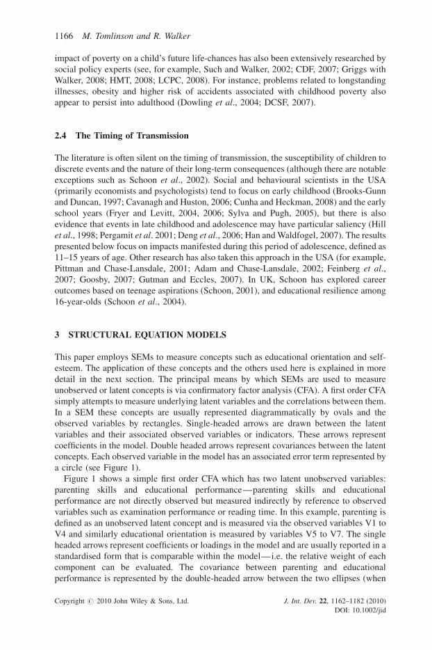
In a SEM these concepts are usually represented diagrammatically by ovals and the

observed variables by rectangles. Single-headed arrows are drawn between the latent

variables and their associated observed variables or indicators. These arrows represent

coefficients in the model. Double headed arrows represent covariances between the latent

concepts. Each observed variable in the model has an associated error term represented by

a circle (see Figure 1).

Figure 1 shows a simple first order CFA which has two latent unobserved variables:

parenting skills and educational performance—parenting skills and educational

performance are not directly observed but measured indirectly by reference to observed

variables such as examination performance or reading time. In this example, parenting is

defined as an unobserved latent concept and is measured via the observed variables V1 to

V4 and similarly educational orientation is measured by variables V5 to V7. The single

headed arrows represent coefficients or loadings in the model and are usually reported in a

standardised form that is comparable within the model—i.e. the relative weight of each

component can be evaluated. The covariance between parenting and educational

performance is represented by the double-headed arrow between the two ellipses (when


DOI: 10.1002/jid

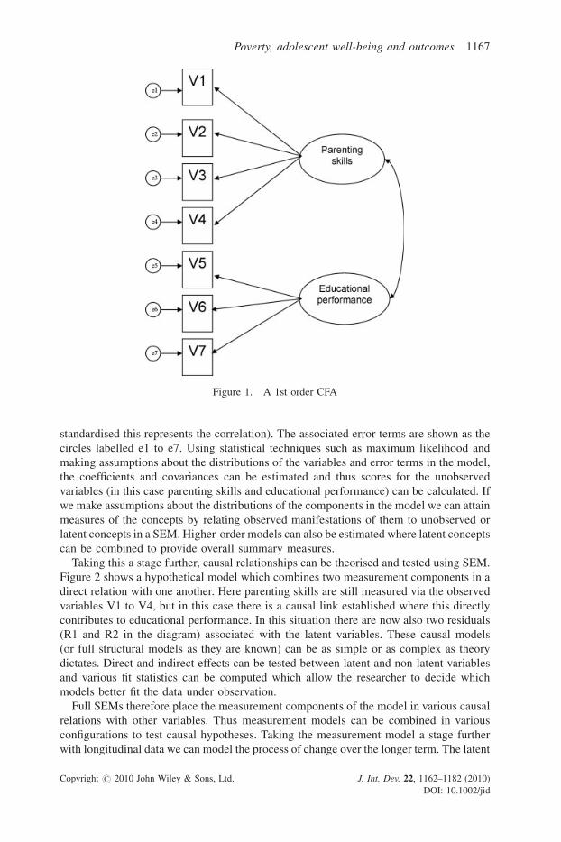
Figure 1. A 1st order CFA


standardised this represents the correlation). The associated error terms are shown as the

circles labelled e1 to e7. Using statistical techniques such as maximum likelihood and

making assumptions about the distributions of the variables and error terms in the model,

the coefficients and covariances can be estimated and thus scores for the unobserved

variables (in this case parenting skills and educational performance) can be calculated. If

we make assumptions about the distributions of the components in the model we can attain

measures of the concepts by relating observed manifestations of them to unobserved or

latent concepts in a SEM. Higher-order models can also be estimated where latent concepts

can be combined to provide overall summary measures.

Taking this a stage further, causal relationships can be theorised and tested using SEM.

Figure 2 shows a hypothetical model which combines two measurement components in a

direct relation with one another. Here parenting skills are still measured via the observed

variables V1 to V4, but in this case there is a causal link established where this directly

contributes to educational performance. In this situation there are now also two residuals

(R1 and R2 in the diagram) associated with the latent variables. These causal models

(or full structural models as they are known) can be as simple or as complex as theory

dictates. Direct and indirect effects can be tested between latent and non-latent variables

and various fit statistics can be computed which allow the researcher to decide which

models better fit the data under observation.

Full SEMs therefore place the measurement components of the model in various causal

relations with other variables. Thus measurement models can be combined in various

configurations to test causal hypotheses. Taking the measurement model a stage further

with longitudinal data we can model the process of change over the longer term. The latent


DOI: 10.1002/jid

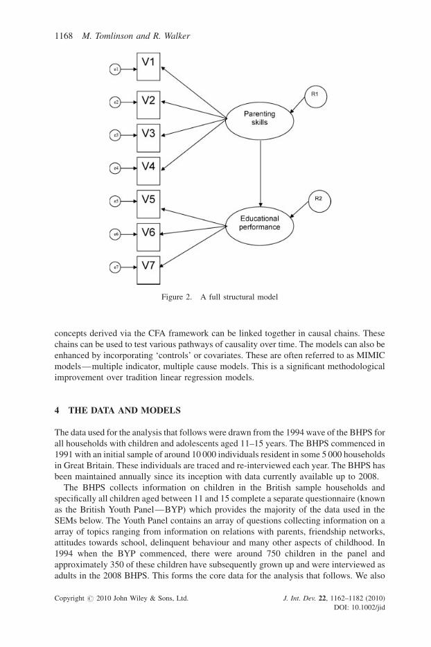
Figure 2. A full structural model


concepts derived via the CFA framework can be linked together in causal chains. These

chains can be used to test various pathways of causality over time. The models can also be

enhanced by incorporating ‘controls’ or covariates. These are often referred to as MIMIC

models—multiple indicator, multiple cause models. This is a significant methodological

improvement over tradition linear regression models.

4 THE DATA AND MODELS

The data used for the analysis that follows were drawn from the 1994 wave of the BHPS for

all households with children and adolescents aged 11–15 years. The BHPS commenced in

1991 with an initial sample of around 10 000 individuals resident in some 5 000 households

in Great Britain. These individuals are traced and re-interviewed each year. The BHPS has

been maintained annually since its inception with data currently available up to 2008.

The BHPS collects information on children in the British sample households and

specifically all children aged between 11 and 15 complete a separate questionnaire (known

as the British Youth Panel—BYP) which provides the majority of the data used in the

SEMs below. The Youth Panel contains an array of questions collecting information on a

array of topics ranging from information on relations with parents, friendship networks,

attitudes towards school, delinquent behaviour and many other aspects of childhood. In

1994 when the BYP commenced, there were around 750 children in the panel and

approximately 350 of these children have subsequently grown up and were interviewed as

adults in the 2008 BHPS. This forms the core data for the analysis that follows. We also


DOI: 10.1002/jid


estimate models from pooled data from the first three waves of the BYP which enabled the

sample size to be increased.

By linking together household level data from the 1994 BHPS to the individual data

from the 1994 BYP it is possible to include data on income, financial strain, parental

characteristics and poverty in the models. Furthermore by combining the BYP with the

data from later waves of the BHPS (in this case as late as 2008) childhood-level variables

can be linked with outcomes relating to educational attainment and labour market

participation in adulthood. By 2008, child respondents in the 1994 BYP were aged between

25 and 29 years old.

This type of analysis has two potential problems. First, there is a significant level of

attrition. We lose approximately half of the children between 1994 and 2008. However, an

examination of the households lost to attrition showed that there were no obvious

differences in the characteristics of these households when compared with those that

remained in the panel (whether the comparison was made by parental education,

occupation, housing tenure, employment status or household structure). Moreover, models

estimated using just the 1994 BYP (excluding the 2008 outcome variables) produce very

similar results to the restricted attrition based sample and have much higher numbers of

cases. This gives us confidence that the estimates derived from the structural models of

childhood experience are not influenced very much by attrition.

The second problem relates to the pooled data from 1994 to 1996 since cases in this

analysis are not independent as children are repeatedly interviewed over two or three

waves. There are two possible routes available to deal with this. One is to apply multi-level

modelling techniques that incorporate fixed or random child-specific effects to account for

unobserved differences between children, and the method, adopted here, that incorporates

robust standard errors that take into account the non-independence of cases.

The 1994 BYP data permit us to measure the following dimensions relating to childhood

well-being (these are summarised in Table 1).

4.1 Parental Guidance

The data from the BYP essentially reflect the child’s view of the world. There are no direct

measures of parenting. However, there are four variables that can be incorporated into a

measure of parental guidance: whether the child tells their parents where they are going

when they go out, whether the parents tell their children where they are going when they go

out, whether the child talks to their mother about things that matter to them, and whether

they talk to the father about things that matter to them. These variables capture the level and

effectiveness of communication between child and parent. All are measured on a 4-point

scale and, if the child respondent does not have a mother (or father), the latter two variables

are coded as the lowest category.

4.2 Self-esteem

Self-esteem is measured using six observed variables: whether the child feels that they have

good qualities, are likeable, how they feel about their appearance, their friends, life in

general and their schoolwork. The first two are measured on a 4-point scale and the rest on a

7-point scale.


DOI: 10.1002/jid

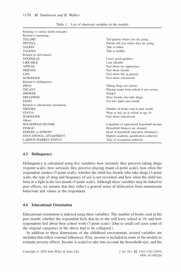
Table 1. List of observed variables in the models

Relating to various latent concepts:

Related to parenting:

TELLPRT Tell parents where you are going

PRTTELL Parents tell you where they are going

TALKPA Talk to father

TALKMA Talk to mother

Related to self-esteem:

GOODQUAL I have good qualities

LIKEABLE I am likeable

APPEAR Feel about my appearance

FRIENDS Feel about friends

LIFE Feel about life in general

SCHOOLWK Feel about schoolwork

Related to delinquency:

DRUG Taking drugs not serious

TRUANT Playing truant from school is not serious

SMOKER Smoker

DRUGFRND Have friends who take drugs

FIGHT Got into fights past month

Related to educational orientation:

NBOOKS Number of books read in past month

STAY16 Want to stay on at school at age 16

SCHOOLWK Feel about schoolwork

Others:

HOUSEHOLD INCOME Logarithm of equivalised household income

FINBAD Household finances are strained

EDHOH1 to EDHOH3 Head of household education (dummies)

EDUCATIONAL ATTAINMENT Highest academic qualification achieved

LABOUR MARKET STATUS Type of occupation achieved


4.3 Delinquency

Delinquency is calculated using five variables: how seriously they perceive taking drugs

(4-point scale), how seriously they perceive playing truant (4-point scale), how often the

respondent smokes (5-point scale), whether the child has friends who take drugs (3-point

scale, the type of drug and frequency of use is not recorded) and how often the child has

been in a fight in the last month (5-point scale). Although these variables may be linked to

peer effects, we assume that they reflect a general sense of dislocation from mainstream

behaviour and values in the respondent.

4.4 Educational Orientation

Educational orientation is indexed using three variables: The number of books read in the

past month; whether the respondent feels that he or she will leave school at 16; and how

respondents feel about their school work (7-point scale). (Due to small cell sizes some of

the original categories in the above had to be collapsed.)

In addition to these dimensions of the childhood environment, several variables are

included that reflect external influences. First, income is included in some of the models to

estimate poverty effects. Income is scaled to take into account the household size, and the


DOI: 10.1002/jid


logarithm taken to ensure that the distribution is not strongly skewed which interferes with

statistical estimation. To capture financial strain a dummy variable is included (FINBAD)

that is set to one if the household is not at least ‘getting by’ financially. To capture parental

endowments the educational level of the household head is included as three dummies.

EDHOH1 for ordinary/GCSE level, EDHOH2 for college/advanced level and EDHOH3

for further/higher level education (the base category is therefore no or only CSE-level

education). The head is used as a proxy for the household as a whole for, while other adults

in the household might be more suitable candidates, which particular adult would be best

cannot be ascertained. Finally the outcome variables in 2008 include educational

attainment and labour market status. Educational outcome is derived as a 4-point scale:

1: N

Cop

o education or CSE level (a low quality minimal educational qualification).

2: G
CSE level (a standard educational qualification for 16 year olds).
3: A
dvanced level (college—normally 18 years of age).
4: P
ost-college education (Further post-college and university education).
Labour market status is measured with respect to the most recent job the respondent had

in the respective year (2006–2008). This is measured on a 3-point scale:

1. S
emi or unskilled occupations.
2. S
killed manual and white-collar workers, armed forces.
3. P
rofessionals, technical and managerial workers.
Following the literature it is hypothesised that parental guidance and delinquency will

both affect educational orientation (although in different directions) and that there is

a direct effect from parental guidance to delinquency (which means, in effect, that

technically delinquency is treated as a moderator variable). It is further proposed that the

educational orientation of the child will have consequences for several outcomes.

Immediately, it will positively affect self-esteem. Again this is in accordance with

numerous behavioural studies as already discussed, but it is important to note the direction

of the effect for, when educational orientation is modelled as a consequence of self-esteem,

this relationship is not significant. In the longer term, having a positive educational

orientation in adolescence will result in higher educational attainment and improved

employment status in adulthood as suggested by much of the literature on the transmission

of disadvantage. The advantage of the approach taken here is that there is no reliance on

linear regression models where all the variables are simply included as determinants of

the individual outcomes. It is possible, using SEM, to determine the real structural

relationships between different elements of childhood and how they affect outcomes in

both the present and future simultaneously. In addition, we control for household income,

endowments and financial strain in several models to assess the potential influence of

household poverty and parental assets. Numerous alternative models were tested and

assessed and the best fit statistics indicated the configuration presented here was the one

best supported by the data.

5 RESULTS

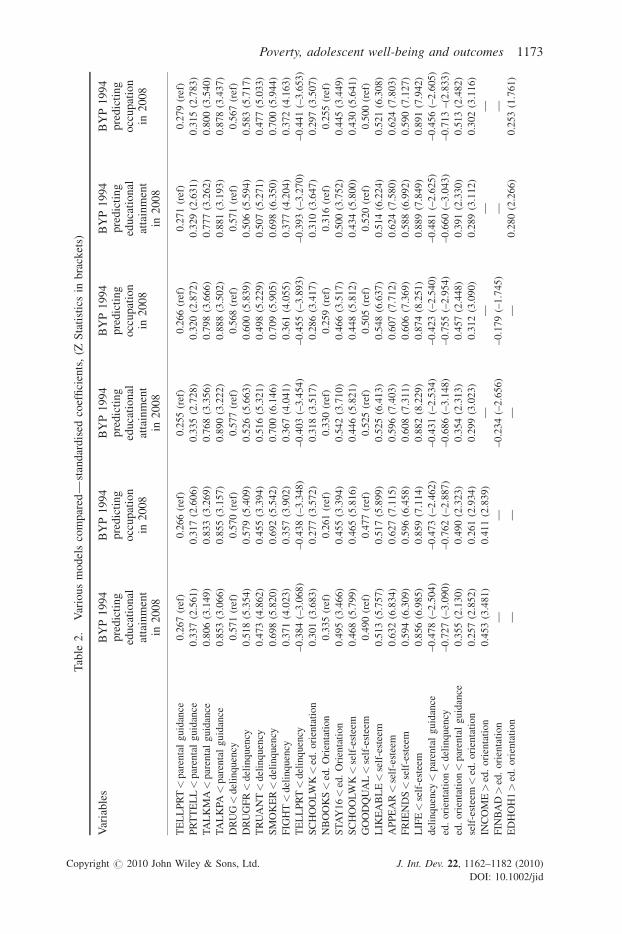
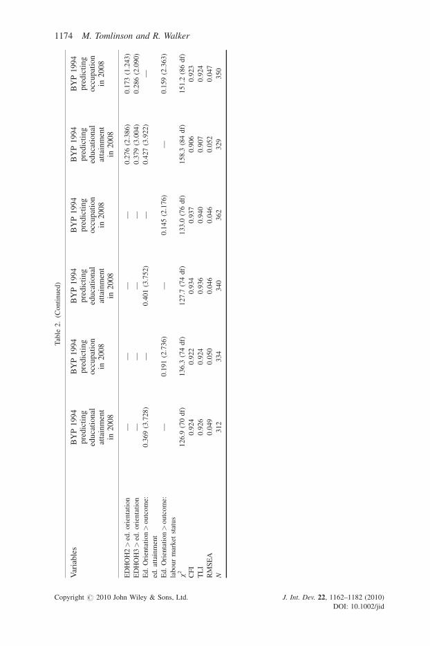
Figure 3 shows the results of a typical model relating outcomes in 2008 to circumstances in

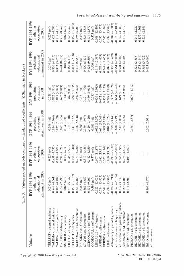
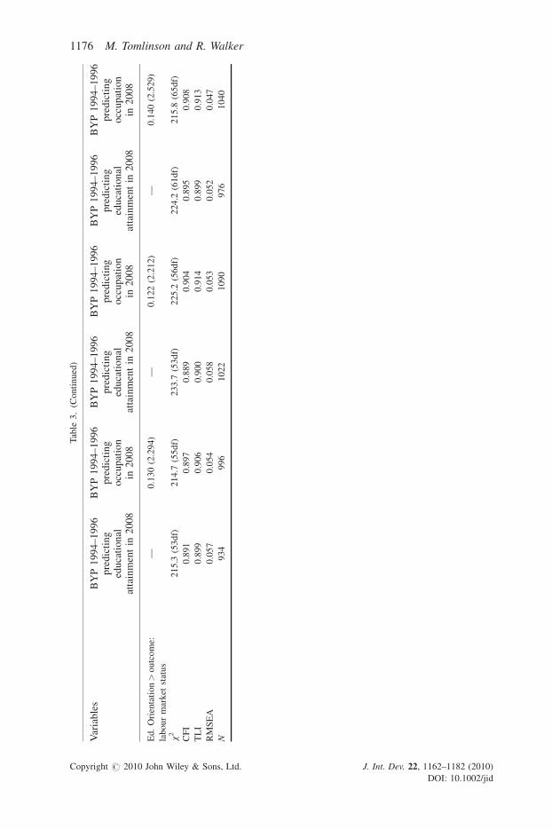
1994. More models with coefficients and Z statistics based on the 1994 data are shown in

Tables 2 and 3 for pooled data for 1994–1996. In the tables the standardized coefficients

yright # 2010 John Wiley & Sons, Ltd. J. Int. Dev. 22, 1162–1182 (2010)

DOI: 10.1002/jid

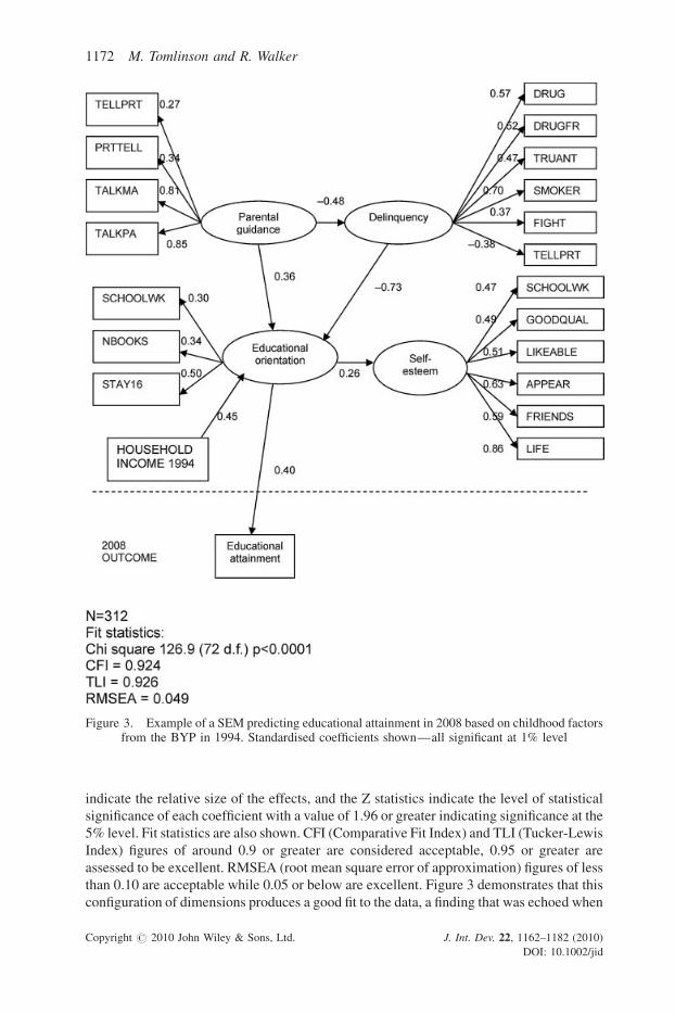
Figure 3. Example of a SEM predicting educational attainment in 2008 based on childhood factorsfrom the BYP in 1994. Standardised coefficients shown—all significant at 1% level


indicate the relative size of the effects, and the Z statistics indicate the level of statistical

significance of each coefficient with a value of 1.96 or greater indicating significance at the

5% level. Fit statistics are also shown. CFI (Comparative Fit Index) and TLI (Tucker-Lewis

Index) figures of around 0.9 or greater are considered acceptable, 0.95 or greater are

assessed to be excellent. RMSEA (root mean square error of approximation) figures of less

than 0.10 are acceptable while 0.05 or below are excellent. Figure 3 demonstrates that this

configuration of dimensions produces a good fit to the data, a finding that was echoed when


DOI: 10.1002/jid

Tab

le2

.V

ario

us

mo

del

sco

mp

ared

—st

and

ard

ised

coef

fici

ents

,(Z

Sta

tist

ics

inb

rack

ets)

Var

iab

les

BY

P1

99

4p

red

icti

ng

edu

cati

on

alat

tain

men

tin

20

08

BY

P1

99

4p

red

icti

ng

occ

up

atio

nin

20

08

BY

P1

99

4p

red

icti

ng

edu

cati

on

alat

tain

men

tin

20

08

BY

P1

99

4p

red

icti

ng

occ

up

atio

nin

20

08

BY

P1

99

4p

red

icti

ng

edu

cati

on

alat

tain

men

tin

20

08

BY

P1

99

4p

red

icti

ng

occ

up

atio

nin

20

08

TE

LL

PR

T<

par

enta

lg

uid

ance

0.2

67

(ref

)0

.266

(ref

)0

.255

(ref

)0

.266

(ref

)0

.271

(ref

)0

.279

(ref

)

PR

TT

EL

L<

par

enta

lg

uid

ance

0.3

37

(2.5

61)

0.3

17

(2.6

06)

0.3

35

(2.7

28

)0

.32

0(2

.87

2)

0.3

29

(2.6

31

)0

.315

(2.7

83)

TA

LK

MA<

par

enta

lg

uid

ance

0.8

06

(3.1

49)

0.8

33

(3.2

69)

0.7

68

(3.3

56

)0

.79

8(3

.66

6)

0.7

77

(3.2

62

)0

.800

(3.5

40)

TA

LK

PA<

par

enta

lg

uid

ance

0.8

53

(3.0

66)

0.8

55

(3.1

57)

0.8

90

(3.2

22

)0

.88

8(3

.50

2)

0.8

81

(3.1

93

)0

.878

(3.4

37)

DR

UG<

del

inq

uen

cy0

.57

1(r

ef)

0.5

70

(ref

)0

.577

(ref

)0

.568

(ref

)0

.571

(ref

)0

.567

(ref

)

DR

UG

FR<

del

inq

uen

cy0

.518

(5.3

54)

0.5

79

(5.4

09)

0.5

26

(5.6

63

)0

.60

0(5

.83

9)

0.5

06

(5.5

94

)0

.583

(5.7

17)

TR

UA

NT<

del

inq

uen

cy0

.473

(4.8

62)

0.4

55

(3.3

94)

0.5

16

(5.3

21

)0

.49

8(5

.22

9)

0.5

07

(5.2

71

)0

.477

(5.0

33)

SM

OK

ER<

del

inq

uen

cy0

.698

(5.8

20)

0.6

92

(5.5

42)

0.7

00

(6.1

46

)0

.70

9(5

.90

5)

0.6

98

(6.3

50

)0

.700

(5.9

44)

FIG

HT<

del

inq

uen

cy0

.371

(4.0

23)

0.3

57

(3.9

02)

0.3

67

(4.0

41

)0

.36

1(4

.05

5)

0.3

77

(4.2

04

)0

.372

(4.1

63)

TE

LL

PR

T<

del

inq

uen

cy–

0.3

84

(–3

.068

)–

0.4

38

(–3

.348

)–

0.4

03

(–3

.45

4)

–0

.45

5(–

3.8

93

)–

0.3

93

(–3

.27

0)

–0

.44

1(–

3.6

53

)

SC

HO

OL

WK<

ed.

ori

enta

tion

0.3

01

(3.6

83)

0.2

77

(3.5

72)

0.3

18

(3.5

17)

0.2

86

(3.4

17)

0.3

10

(3.6

47)

0.2

97

(3.5

07)

NB

OO

KS<

ed.

Ori

enta

tio

n0

.33

5(r

ef)

0.2

61

(ref

)0

.330

(ref

)0

.259

(ref

)0

.316

(ref

)0

.255

(ref

)

ST

AY

16<

ed.

Ori

enta

tio

n0

.495

(3.4

66)

0.4

55

(3.3

94)

0.5

42

(3.7

10

)0

.46

6(3

.51

7)

0.5

00

(3.7

52

)0

.445

(3.4

49)

SC

HO

OL

WK<

self

-est

eem

0.4

68

(5.7

99)

0.4

65

(5.8

16)

0.4

46

(5.8

21)

0.4

48

(5.8

12)

0.4

34

(5.8

00)

0.4

30

(5.6

41)

GO

OD

QU

AL<

self

-est

eem

0.4

90

(ref

)0

.477

(ref

)0

.525

(ref

)0

.505

(ref

)0

.520

(ref

)0

.500

(ref

)

LIK

EA

BL

E<

self

-est

eem

0.5

13

(5.7

57)

0.5

17

(5.8

99)

0.5

25

(6.4

13

)0

.54

8(6

.63

7)

0.5

14

(6.2

24

)0

.521

(6.3

08)

AP

PE

AR<

self

-est

eem

0.6

32

(6.8

34)

0.6

27

(7.1

15)

0.5

96

(7.4

03

)0

.60

7(7

.71

2)

0.6

24

(7.5

80

)0

.624

(7.8

03)

FR

IEN

DS<

self

-est

eem

0.5

94

(6.3

09)

0.5

96

(6.4

58)

0.6

08

(7.3

11)

0.6

06

(7.3

69)

0.5

88

(6.9

92)

0.5

90

(7.1

27)

LIF

E<

self

-est

eem

0.8

56

(6.9

85)

0.8

59

(7.1

14)

0.8

82

(8.2

29)

0.8

74

(8.2

51)

0.8

89

(7.8

49)

0.8

91

(7.9

42)

del

inq

uen

cy<

par

enta

lg

uid

ance

–0

.47

8(–

2.5

04

)–

0.4

73

(–2

.462

)–

0.4

31

(–2

.53

4)

–0

.42

3(–

2.5

40

)–

0.4

81

(–2

.62

5)

–0

.45

6(–

2.6

05

)

ed.

ori

enta

tio

n<

del

inq

uen

cy–

0.7

27

(–3

.090

)–

0.7

62

(–2

.887

)–

0.6

86

(–3

.14

8)

–0

.75

5(–

2.9

54

)–

0.6

60

(–3

.04

3)

–0

.71

3–

(2.8

33

)

ed.

ori

enta

tio

n<

par

enta

lg

uid

ance

0.3

55

(2.1

30)

0.4

90

(2.3

23)

0.3

54

(2.3

13

)0

.45

7(2

.44

8)

0.3

91

(2.3

30

)0

.513

(2.4

82)

self

-est

eem<

ed.

ori

enta

tion

0.2

57

(2.8

52)

0.2

61

(2.9

34)

0.2

99

(3.0

23)

0.3

12

(3.0

90)

0.2

89

(3.1

12)

0.3

02

(3.1

16)

INC

OM

E>

ed.

ori

enta

tion

0.4

53

(3.4

81)

0.4

11

(2.8

39)

——

——

FIN

BA

D>

ed.

ori

enta

tio

n—

—–

0.2

34

(–2

.65

6)

–0

.17

9(–

1.7

45

)—

—

ED

HO

H1>

ed.

ori

enta

tio

n—

——

—0

.280

(2.2

66

)0

.253

(1.7

61)

(Co

nti

nu

es)


Copyright # 2010 John Wiley & Sons, Ltd. J. Int. Dev. 22, 1162–1182 (2010

DOI: 10.1002/jid

)

Tab

le2

.(C

onti

nu

ed)

Var

iab

les

BY

P1

99

4p

red

icti

ng

edu

cati

on

alat

tain

men

tin

20

08

BY

P1

99

4p

red

icti

ng

occ

up

atio

nin

20

08

BY

P1

99

4p

red

icti

ng

edu

cati

on

alat

tain

men

tin

20

08

BY

P1

99

4pre

dic

ting

occ

up

atio

nin

20

08

BY

P1

99

4p

red

icti

ng

edu

cati

on

alat

tain

men

tin

20

08

BY

P1

99

4p

red

icti

ng

occ

up

atio

nin

20

08

ED

HO

H2>

ed.

ori

enta

tion

——

——

0.2

76

(2.3

86)

0.1

73

(1.2

43)

ED

HO

H3>

ed.

ori

enta

tion

——

——

0.3

79

(3.0

04)

0.2

86

(2.0

90)

Ed

.O

rien

tati

on>

ou

tco

me:

ed.

atta

inm

ent

0.3

69

(3.7

28

)—

0.4

01

(3.7

52)

—0

.427

(3.9

22)

—

Ed

.O

rien

tati

on>

ou

tco

me:

lab

ou

rm

ark

etst

atu

s

—0

.19

1(2

.73

6)

—0

.145

(2.1

76)

—0

.159

(2.3

63)

x2

12

6.9

(70

df)

13

6.3

(74

df)

12

7.7

(74

df)

13

3.0

(76

df)

15

8.3

(84

df)

15

1.2

(86

df)

CF

I0

.92

40

.922

0.9

34

0.9

37

0.9

06

0.9

23

TL

I0

.92

60

.924

0.9

36

0.9

40

0.9

07

0.9

24

RM

SE

A0

.04

90

.050

0.0

46

0.0

46

0.0

52

0.0

47

N3

12

33

43

40

36

23

29

35

0


DOI: 10.1002/jid


Tab

le3

.V

ario

us

po

ole

dm

od

els

com

par

ed—

stan

dar

dis

edco

effi

cien

ts,

(ZS

tati

stic

sin

bra

cket

s)

Var

iab

les

BY

P1

99

4–

19

96

pre

dic

tin

ged

uca

tio

nal

atta

inm

ent

in2

00

8

BY

P1

99

4–

19

96

pre

dic

tin

go

ccu

pat

ion

in2

00

8

BY

P1

99

4–

19

96

pre

dic

tin

ged

uca

tio

nal

atta

inm

ent

in2

00

8

BY

P1

99

4–

19

96

pre

dic

tin

go

ccu

pat

ion

in2

00

8

BY

P1

99

4–

19

96

pre

dic

tin

ged

uca

tio

nal

atta

inm

ent

in2

00

8

BY

P1

99

4–

19

96

pre

dic

tin

go

ccu

pat

ion

in2

00

8

TE

LL

PR

T<

par

enta

lg

uid

ance

0.2

40

(ref

)0

.229

(ref

)0

.249

(ref

)0

.22

8(r

ef)

0.2

44

(ref

)0

.227

(ref

)

TA

LK

MA<

par

enta

lg

uid

ance

0.8

49

(4.6

61

)0

.851

(4.5

92

)0

.814

(5.0

84)

0.8

32

(4.8

01)

0.8

26

(4.9

15)

0.8

27

(4.6

93

)

TA

LK

PA<

par

enta

lg

uid

ance

0.7

86

(4.7

89

)0

.794

(4.7

01

)0

.827

(5.1

69)

0.8

25

(4.8

95)

0.8

13

(5.0

70)

0.8

19

(4.8

13

)

DR

UG

FR<

del

inq

uen

cy0

.65

7(7

.89

5)

0.6

94

(8.3

21

)0

.672

(8.3

55)

0.6

97

(8.8

19)

0.6

94

(8.6

27)

0.7

18

(8.9

67

)

SM

OK

ER<

del

inq

uen

cy0

.842

(ref

)0

.839

(ref

)0

.848

(ref

)0

.84

2(r

ef)

0.8

48

(ref

)0

.841

(ref

)

FIG

HT<

del

inq

uen

cy0

.37

0(5

.84

7)

0.3

46

(5.6

67

)0

.362

(6.1

10)

0.3

46

(6.0

01)

0.3

61

(6.1

33)

0.3

45

(5.9

62

)

TE

LL

PR

T<

del

inq

uen

cy–

0.4

50

(–7

.18

2)

–0

.45

4(–

7.4

01

)–

0.4

41

(–7

.529

)–

0.4

56

(–7

.935

)–

0.4

43

(–7

.508

)–

0.4

59

(–7

.88

5)

SC

HO

OL

WK<

ed.

ori

enta

tio

n0

.32

0(5

.46

8)

0.2

79

(5.2

80

)0

.326

(5.5

08)

0.2

86

(5.4

25)

0.3

36

(5.9

58)

0.2

95

(5.7

03

)

NB

OO

KS<

ed.

Ori

enta

tio

n0

.367

(ref

)0

.330

(ref

)0

.363

(ref

)0

.33

1(r

ef)

0.3

69

(ref

)0

.330

(ref

)

ST

AY

16<

ed.

Ori

enta

tio

n0

.36

7(4

.65

9)

0.3

13

(4.4

55

)0

.379

(4.9

67)

0.3

21

(4.7

90)

0.4

00

(5.1

32)

0.3

26

(4.8

35

)

SC

HO

OL

WK<

self

-est

eem

0.4

37

(9.4

60

)0

.442

(8.9

50

)0

.429

(9.4

20)

0.4

39

(9.0

64)

0.4

26

(9.5

06)

0.4

34

(8.8

79

)

GO

OD

QU

AL<

self

-est

eem

0.5

89

(ref

)0.5

70

(ref

)0.6

01

(ref

)0.5

85

(ref

)0.5

90

(ref

)0.5

75

(ref

)

LIK

EA

BL

E<

self

-est

eem

0.6

23

(12

.02

5)

0.6

07

(11

.87

9)

0.6

32

(13

.072

)0

.626

(13

.083

)0

.619

(12

.387

)0

.60

8(1

2.4

05

)

AP

PE

AR<

self

-est

eem

0.6

84

(13

.92

3)

0.6

82

(13

.41

3)

0.6

71

(14

.668

)0

.672

(14

.420

)0

.687

(14

.479

)0

.69

5(1

3.9

77

)

FR

IEN

DS<

self

-est

eem

0.5

48

(11

.26

3)

0.5

52

(11

.14

8)

0.5

49

(12

.196

)0

.555

(12

.125

)0

.544

(11

.655

)0

.54

7(1

1.5

60

)

LIF

E<

self

-est

eem

0.7

94

(13

.86

3)

0.8

00

(13

.59

0)

0.8

10

(15

.324

)0

.798

(14

.879

)0

.809

(14

.342

)0

.79

9(1

3.9

60

)

del

inq

uen

cy<

par

enta

lg

uid

ance

–0

.29

9(–

3.2

13

)–

0.2

90

(–3

.10

5)

–0

.29

9(–

3.4

43

)–

0.3

02

(–3

.328

)–

0.3

10

(–3

.459

)–

0.3

07

(–3

.31

7)

ed.

ori

enta

tio

n<

del

inq

uen

cy–

0.6

40

(–5

.15

6)

–0

.66

6(–

5.0

29

)–

0.6

18

(–5

.193

)–

0.6

64

(–5

.268

)–

0.5

64

(–5

.030

)–

0.6

28

(–5

.01

1)

ed.

ori

enta

tio

n<

par

enta

lg

uid

ance

0.5

37

(3.8

32

)0

.666

(3.9

99

)0

.512

(4.0

23)

0.6

19

(4.1

02)

0.5

04

(4.0

09)

0.6

49

(4.0

89

)

self

-est

eem<

ed.

ori

enta

tio

n0

.25

8(4

.10

3)

0.2

76

(4.6

12

)0

.284

(4.4

65)

0.3

04

(5.0

86)

0.2

56

(4.2

05)

0.2

79

(4.8

12

)

INC

OM

E>

ed.

ori

enta

tio

n0

.21

4(2

.50

0)

0.1

03

(1.1

07

)—

——

—

FIN

BA

D>

ed.

ori

enta

tion

——

–0.1

85

(–2.8

71)

–0.0

97

(–1.3

12)

——

ED

HO

H1>

ed.

ori

enta

tion

——

——

0.3

21

(3.3

58)

0.2

46

(2.2

29)

ED

HO

H2>

ed.

ori

enta

tion

——

——

0.2

73

(3.1

44)

0.1

52

(1.5

01)

ED

HO

H3>

ed.

ori

enta

tion

——

——

0.3

62

(3.9

22)

0.2

26

(2.1

46)

Ed

.O

rien

tati

on>

ou

tco

me:

ed.

atta

inm

ent

0.3

64

(4.9

76

)—

0.3

62

(5.0

71)

—0

.433

(5.6

66)

— (Co

nti

nu

es)



DOI: 10.1002/jid

)

Tab

le3

.(C

onti

nu

ed)

Var

iab

les

BY

P1

99

4–

19

96

pre

dic

tin

ged

uca

tio

nal

atta

inm

ent

in2

00

8

BY

P1

99

4–

19

96

pre

dic

tin

go

ccu

pat

ion

in2

00

8

BY

P1

99

4–

19

96

pre

dic

tin

ged

uca

tio

nal

atta

inm

ent

in2

00

8

BY

P1

99

4–

19

96

pre

dic

tin

go

ccu

pat

ion

in2

00

8

BY

P1

99

4–

19

96

pre

dic

tin

ged

uca

tio

nal

atta

inm

ent

in2

00

8

BY

P1

99

4–

19

96

pre

dic

tin

go

ccu

pat

ion

in2

00

8

Ed

.O

rien

tati

on>

ou

tco

me:

lab

ou

rm

ark

etst

atu

s

—0

.13

0(2

.29

4)

—0

.122

(2.2

12)

—0

.140

(2.5

29)

x2

21

5.3

(53

df)

21

4.7

(55

df)

23

3.7

(53

df)

22

5.2

(56

df)

22

4.2

(61

df)

21

5.8

(65

df)

CF

I0

.891

0.8

97

0.8

89

0.9

04

0.8

95

0.9

08

TL

I0

.899

0.9

06

0.9

00

0.9

14

0.8

99

0.9

13

RM

SE

A0

.057

0.0

54

0.0

58

0.0

53

0.0

52

0.0

47

N9

34

99

61

02

21

09

09

76

10

40


DOI: 10.1002/jid


)


the 2008 outcome variables were excluded to increase the sample size and deal with the

impact of attrition as previously affirmed.

Parental guidance reduces delinquent behaviour in all the models; and parental guidance

and delinquency both have an impact on educational orientation. Parenting positively

increases educational orientation while delinquent behaviour decreases it. In terms of

outcomes it is clear that educational orientation in turn positively affects the three variables

of interest. It significantly contributes to enhanced self-esteem in childhood in all the

models and increases the likelihood of higher educational attainment and better labour

market status in adulthood. Presenting the same findings slightly differently, delinquency is

seen to have a negative impact on all three measures of achievement through its effect on

educational orientation. However, parental guidance can serve to reduce delinquent

behaviour while also directly enhancing a child’s educational orientation.

We also estimated models with controls for age and gender on all the latent concepts

(these models are not reported here). Although the fit statistics were reduced, the models

confirmed that, while delinquency increased with age, neither education nor self-esteem

varied between the ages of 11 and 16 and parental guidance was similarly invariant by age.

However, being a girl increased educational orientation and parental guidance while being

female also reduced self-esteem. The essence is that although there are gender differences,

for instance, in terms of self-esteem and educational orientation, they do not fundamentally

alter the logic of the model. In other words although gender may reduce a girl’s self-esteem

relative to a boy’s (all other things being equal) there is still a statistically significant

relationship between the factors conceptualised in the models which does not change.

Higher educational orientation will still lead to higher self-esteem despite gender.

In addition to this, from an examination of the controlling variables it is also evident that

income has an effect on educational orientation. Thus the poorer the household that the

child lives in the less likely it will be that the child will have a high educational orientation

(with the consequence that they will eventually perform less well in terms of final

educational attainment and labour market status). Financial strain has a similar impact, but

only in the models predicting educational achievement. Thus children in those households

that are not coping well with their finances are also statistically less likely to have high

educational orientation and to succeed in leaving education with high qualifications

Therefore even in households that may technically not be poor, but are nevertheless in

financial difficulty, children have a tendency to perform less well at school. Finally, as

would be expected, parent’s education is found to be associated with their child’s

educational outlook (Tables 2 and 3). Children in households headed by more educated

adults will have a greater chance of having a higher educational orientation.

However, the results of models with these controlling variables need to be treated with a

degree of caution. When income, education of the head of household and financial strain

are all included in the model together, only education tends to remain significant. This is no

doubt because there are very high correlations between these three variables. Thus it is

difficult to say with certainty, taking the income models in isolation, whether poverty is the

direct cause of the fall in educational orientation or whether it is due to other factors such as

status, class and education.

Nevertheless, the models do demonstrate that parental guidance and low levels of

delinquency can potentially offset some of the negative effects of low income and financial

hardship, although the routes by which this occurs remain to be investigated. In other words

(and in line with much of the literature) if a child in a poor household has dependable

parents and avoids delinquency then they will have a better chance of succeeding in the


DOI: 10.1002/jid


present (in terms of self-esteem) and in the future (in terms of crucial adult outcomes). This

is not to say that the benefits of good parenting outweigh the effects of poverty and

household financial pressures on children; indeed, comparing the size of the coefficients

shown in Figure 3 suggests that parental engagement is not in itself sufficient to prevent

delinquency or to neutralise its negative impact on a child’s educational orientation; and

also that extra income may have a more powerful positive effect on this aspect of child

well-being than good parenting alone. However, what is without doubt is that parenting,

access to resources via income and other parental endowments and the absence of

delinquent behaviour are all part of the explanation of what constitutes a good childhood.

6 CONCLUSIONS

It has been demonstrated that a SEM of adolescent circumstances and the transmission of

disadvantage can be used to reveal the potential impact of various individual and contextual

attributes on adult outcomes. If we take educational orientation and performance to be at

the crux of early determinants of academic and labour market performance then it has been

shown that parental guidance, parental endowments, household finances and the avoidance

of delinquency all play a significant part in the process. However, it is no simple matter to

determine which of these factors is more or less important for the child not least because

they tend to work in concert. One conclusion from these observations is that any policy

programme to address these issues would be more successful if it employed a

comprehensive package that includes poverty alleviation, alongside educational assistance,

improving parental relations in terms of communication, and financial support in order to

assuage the impact of disadvantage on future life chances in children. Not only is it likely to

be necessary to tackle multiple impediments but the effectiveness of one intervention may

be lessened if another is not in place.

The results suggest that dealing with low income alone will only be a partial solution at

best to problems of social mobility and the underachievement of children. How far these

results prove pertinent in other contexts particularly developing nations has yet to be

determined. However, there is a growing evidence of the cumulative effects of

disadvantage across the world and evidence is emerging that the influences and well-

being of children in the here and now are powerful predictors of their future life chances

irrespective of where they live (Harper and Marcus, 2003; Walker et al., 2007; Engle and

Black, 2008; Behman et al., 2010). The increasing availability of panel data, such as that in

Mexico and Guatemala, is beginning to facilitate research into the longer-term scarring

effects of poverty and disadvantage on children that in all probability reduce opportunities

and restrict constructive outcomes (Akee et al., 2010; Behman et al., 2010). Moreover, the

unique contribution of the techniques employed in this research is that they allow the

simultaneous investigation of the relative strengths of different childhood influences on

multiple future outcomes and permit the causal pathways to be validated. Not only does

this extend the power of explanatory models, the results may also help policymakers to

ascertain factors to which they should focus more resources and in what specific contexts

resources are constrained. For example, from the coefficients in our models it appears that

income is more important than parental guidance in shaping a child’s educational

orientation but that delinquency has the largest overall impact. This may not be the case in

other cultures. Perhaps inevitably, the results presented raise more questions than can be

answered with the current level of analysis, which is primarily cross-sectional. A deeper


DOI: 10.1002/jid


investigation of the longitudinal aspects of the BYP should enable us to disentangle to a

greater extent the true causes and determinants of childhood well-being and ultimately

critical outcomes later in life. Future research is planned to exploit the longitudinal nature

of the BYP and explore other controlling factors by including the personality of the child,

other parental characteristics and the child’s environmental situation in terms of

neighbourhood and housing. This will be undertaken in tandem with examining trajectories

of well-being in adolescence and their impact on later outcomes using a latent growth

modelling framework which takes the SEM method further by incorporating well-being

and poverty dynamics. Crucially a more multi-level approach to the data which can take

unobserved personal and household characteristics into account will take us another step

further in our understanding of the mechanisms which restrict children from realising their

ultimate potential.

REFERENCES

Aber JL, Jones SM, Cohen J. 2000. The impact of poverty on the mental health and development of

very young children. In Handbook of Infant Mental Health, 2nd edn, Zeanah CH, Jr (ed.). Guilford

Press: New York.

Adam EK, Chase-Lansdale PL. 2002. Home sweet home(s): parental separations, residential moves,

and adjustment problems in low-income adolescent girls. Developmental Psychology 38(5): 792–805.

Akee R, Copeland W, Keeler G, Angold A, Costello J. 2010. Parents’ incomes and children’s

outcomes: a quasi-experiment. American Economic Journal: Applied Economics 2(1): 86–115.

Barth R, Wildfire J, Green R. 2006. Placement into foster care and the interplay of urbanicity, Child

behavior problems, and poverty. American Journal of Orthopsychiatry 76(3): 358–366.

Behman J, Murphy A, Quisumbing A, Yount K. 2010. Mothers’ human capital and the intergenera-

tional transmission of poverty: the impact of mothers’ intellectual human capital and long-run

nutritional status on children’s human capital Guatemala. Working Paper 160, Chronic Poverty

Research Centre: Manchester.

Blanden J. 2006. ‘Bucking the trend’: what enables those who are disadvantaged in childhood to

succeed later in life? DWP Working Paper 31.

Blanden J, Gibbons S. 2006. The persistence of poverty across generations: a view from two British

cohorts. Policy Press: Bristol.

Blanden J, Gregg P. 2004. Family income and educational attainment: a review of approaches and

evidence from Britain. Oxford Review of Economic Policy 20(2): 245–263.

Bradshaw J, Hoelscher P, Richardson D. 2007. An index of child well-being in the European union.

Social Indicators Research 80: 133–177.

Bradshaw J, Mayhew E (eds). 2005. The Well-being of Children in the UK, 2nd edn. Save the

Children: London.

Breen R, Goldthorpe JH. 1999. Class inequality and meritocracy: a critique of Saunders and an

alternative analysis. British Journal of Sociology 50(1): 1–27.

Brooks-Gunn J, Duncan GJ. 1997. The effects of poverty on children. Future of Children 7: 55–71.

Camfield L, Streuli N, Woodhead M. 2009. ‘What’s the Use of ‘Well-Being’ in Contexts of Child

Poverty? Approaches to Research, Monitoring and Children’s Participation’. The International

Journal of Children’s Rights 17(1): 65–109.

Cavanagh SE, Huston A. 2006. Family instability and children’s early problem behavior. Social

Forces 85: 575–605.

CDF. 2007. Child Poverty in America. Children’s Defense Fund: Washington, DC.


DOI: 10.1002/jid


Clarke-Stewart A, Brentano C. 2006. Divorce: Causes and Consequences. Yale University Press:

Newhaven.

Craine S. 1997. The ‘black magic roundabout’: cyclical transitions social exclusion and alternative

careers. In Youth, the ‘Underclass’ and Social Exclusion, McDonald RM (ed.). Routledge: London.

Cunha F, Heckman JJ. 2008. Formulating, Identifying and Estimating the Technology of Cognitive

and Noncognitive Skill Formation. Journal of Human Resources, 43: (4).

Davies J, Brember I. 1998. National curriculum testing and self-esteem in year 2—the first five years:

a cross-sectional study. Educational Psychology 18: 365–375.

Davies J, Brember I. 1999. Reading and mathematics attainments and self-esteem in years 2 and 6: an

eight year cross-sectional study. Educational Studies 25: 145–157.

DCSF. 2007. Children and Young People Today, Evidence to Support the Development of the

Children’s Plan. Department for Children, Schools and Families: London.

Dean H. 1997. Underclassed or undermined? Young people and social citizenship. In McDonald RM

(ed.). Youth, the ‘Underclass’ and Social Exclusion. Routledge; London.

Deng S, Lopez V, Roosa MW, Ryu E, Burrell GL, Tein J, Crowder S. 2006. Family processes

mediating the relationship of neighborhood disadvantage to early adolescent internalizing

problems. The Journal of Early Adolescence 26: 206–231.

Dowling H, Joughin C, Logan S, Laing G, Roberts H. 2004. Financial Benefits and Child Health.

Barnardo’s: London.

Emler N. 2001. Self-esteem: The Costs and Causes of Low Self-worth. YPS for the Joseph Rowntree

Foundation: York.

Engle P, Black M. 2008. The effect of poverty on child development and educational outcomes.

Annals of the New York Academy of Sciences 1136: 243–256.

Erikson R, Goldthorpe JH. 2002. Intergenerational inequality: a sociological perspective. Journal of

Economic Perspectives 16(3): 31–44.

Ermisch J, Francesconi M, Pevalin DJ. 2001. Outcomes for Children in Poverty, DWP Research

Report No. 158, Corporate Document Services: Leeds.

Fahmy E. 2006. Youth, poverty and social exclusion. In Pantazis C, Gordon D, Levitas R (eds).

Poverty and Social Exclusion in Britain: The Millennium Survey. The Policy Press: Bristol.

Feinberg ME, Ridenour TA, Greenberg MT. 2007. Aggregating indices of risk and protection for

adolescent behaviour problems: the communities that care youth survey. Journal of Adolescent

Health 40: 506–513.

Flouri E. 2004. Subjective well-being in midlife: the role of involvement of and closeness to parents

in childhood. Journal of Happiness Studies 5: 335–358.

Flouri E, Buchanan A. 2004. Childhood families of homeless and poor adults in Britain: a prospective

study. Journal of Economic Psychology 25: 1–14.

Fryer R, Levitt SD. 2004. Understanding the Black-White test score gap in the first two years of

school. The Review of Economics and Statistics 86: 447–464.

Fryer RG, Levitt SD. 2006. The black-white test score gap through third grade. American Law and

Economics Review 8(2): 249–281.

Gallie D., 1999. ‘Unemployment and Social Exclusion in the European Union’. European Societies

1: 139–167.

Gallie D, Paugam S, Jacobs S. 2003. Unemployment, poverty and social isolation: is there a vicious

circle of social exclusion? European Societies 5(1): 1–32.

Gershoff ET, Aber JL, Raver CC. 2003. Child poverty in the United States: an evidence-based

conceptual framework for programs and policies. In Jacobs F Wertlieb D Lerner RM (eds). Handbook

of Applied Developmental Science: Promoting Positive Child, Adolescent, and Family Development

Through Research, Policies, and Programs, Vol. 2. Sage: Thousand Oaks, CA, pp. 81–136.


DOI: 10.1002/jid


Goosby BJ. 2007. Poverty duration, maternal psychological resources, and adolescent socioemo-

tional outcomes. Journal of Family Issues 28(8): 1113–1134.

Griggs J, Walker R, 2008. The Costs of Child Poverty for Individuals and Society: A Literature

Review. Joseph Rowntree Foundation: York.

Gutman LM, Eccles JS. 2007. Stage-environment fit during adolescence: Trajectories of family

relations and adolescent outcomes. Developmental Psychology 43(2): 522–537.

Han W-J, Waldfogel J. 2007. Parental work schedules, family process, and early adolescents’ risky

behaviour. Children and Youth Services Review 29: 1249–1266.

Haney P, Durlak JA. 1998. Changing self-esteem in children and adolescents: a meta-analytic review.

Journal of Clinical and Child Psychology 27: 423–433.

Hannon L. 2003. Poverty, delinquency, and educational attainment: cumulative disadvantage or

disadvantage saturation? Sociological Inquiry 73(4): 575–595.

Harper C, Marcus R. 2003. Enduring poverty and the conditions of childhood: lifecourse and

intergenerational poverty transmissions. World Development 31(3): 535–554.

Hill M, Hill D, Walker R. 1998. Intergenerational dynamics in the USA: poverty processes in young

adulthood. In Leisering L, Walker R (eds). The Dynamics of Modern Society: Poverty, Policy and

Welfare. Policy Press: Bristol, pp. 85–107

HMT. 2008. Ending Child Poverty: Everybody’s Business. HM Treasury, HMSO: London.

Hobcraft J. 1998. Intergenerational and life-course transmission of social exclusion: influences and

childhood poverty, family disruption and contact with the police. CASE Paper 15, London School

of Economics.

Istance D, Rees G, Williamson H. 1994. Young People Not in Education, Training or Employment in

South Glamorgan. South Glamorgan TEC/University of Wales: Cardiff.

Katz I, Corlyon J, La Placa V, Hunter S. 2007. The Relationship Between Parenting and Poverty.

Joseph Rowntree Foundation: York.

Lampard R. 1993. An examination of the relationship between marital dissolution and unemploy-

ment. In Social Change and the Experience of Unemployment. Gallie D, Marsh C, Vogler C (eds).

Oxford University Press: Oxford.

Land KC, Lamb VL, Meadows SO, Taylor A. 2006. Measuring trends in child well-being: An

evidence-based approach. Social Indicators Research 80: 105–132.

Layard R, Dunn J. 2009. A Good Childhood: Searching for Values in a Competitive Age. Penguin.

London.

LCPC (London Child Poverty Commission). 2008. Capital Gains: London Child Poverty Commis-

sion Final Report. London Child Poverty Commission.

Lister MRA. 2005. Investing in the citizen-workers of the future. In Child Welfare and Social Policy.

An Essential Reader, Hendrick H (ed.). Policy Press: Bristol.

Lloyd E. 2006. Children, poverty and social exclusion. In Pantazis C, Gordon D, Levitas R (eds).

Poverty and Social Exclusion in Britain: The Millennium Survey. Policy Press: Bristol.

Marsh HW. 1992. Content specificity of relations between academic achievement and academic self-

concept. Journal of Educational Psychology 84: 35–42.

Masten AS. 2001. Ordinary magic: resilience processes in development. American Psychologist 56:

227–238.

Masten AS, Coatsworth JD. 1998. The development of competence in favorable and unfavorable

environments: lessons from research on successful children. American Psychologist 53: 205–220.

Mayall B. 2002. Towards a Sociology for Childhood. Open University Press: Maidenhead.

McCulloch A, Joshi HE. 2001. Neighbourhood and family influences on the cognitive ability of

children in the British National Child Development Study. Social Science and Medicine 53(5):

579–591.


DOI: 10.1002/jid


McLennahan C, Irwing P, Stringer M, Giles M, Wilson R. 2003. Educational differences in self-

perceptions of adolescents in Northern Ireland. International Journal of Behavioral Development

27(6): 513–518.

Monk-Turner E. 1989. Effects of high school delinquency on educational attainment and adult

occupational status. Sociological Perspectives 32: 413–418.

Moore K. 2001. Frameworks for understanding the inter-generational transmission of poverty and

well-being in developing countries. CPRC Working Paper 8, International Development Depart-

ment, University of Birmingham.

Moore K. 2005. Thinking about youth poverty through the lenses of chronic poverty, life-course

poverty and inter-generational poverty. CPRC Working Paper 57, Institute for Development Policy

and Management, University of Manchester.

Paugam S. 1995. The spiral of precariousness: a multidimensional approach to the process of social

disqualification in France. In Room G (ed.). Beyond the Threshold: The Measurement and Analysis

of Social Exclusion. Policy Press: Bristol.

Pergamit M, Huang L, Lane J. 2001. The Long Term Impact of Adolescent Risky Behaviors and

Family Environment. ASPE/DHHS: Washington, DC.

Pittman LD, Chase-Lansdale PL. 2001. African American adolescent girls in impoverished com-

munities: parenting style and adolescent outcomes. Journal of Research on Adolescence, 11(2):

199–224.

Ridge T. 2002. Childhood Poverty and Social Exclusion. The Policy Press: Bristol.

Ross A, Schoon I, Martin P, Sacker A. 2009. Family and nonfamily role configurations in two British

cohorts. Journal of Marriage and Family 71 (February): 1–14.

Schoon I. 2001. Teenage job aspirations and career attainment in adulthood: A 17-year follow-up

study of teenagers who aspired to become scientists, health professionals, or engineers. Inter-

national Journal of Behavioural Development 25(2): 124–132.

Schoon I, Bynner J, Joshi H, Parsons S, Wiggins RD, Sacker A. 2002. The influence of context,

timing, and duration of risk experiences for the passage from childhood to midadulthood. Child

Development 73(5): 1486–1504.

Schoon I, Parsons S, Sacker A. 2004. Socioeconomic adversity, educational resilience, and

subsequent levels of adult adaptation. Journal of Adolescent Research 19(4): 383–404.

Stewart K. 2005. Towards and equal start? Addressing childhood poverty and deprivation. In Hills J,

Stewart K (eds). A More Equal Society? New Labour, Poverty, Inequality and Exclusion. Policy

Press: Bristol.

Such E, Walker R. 2002. Falling behind? Research on transmitted deprivation. Benefits 10(3): 185–

192.

Sylva K, Pugh G. 2005. Transforming the early years in England. Oxford Review of Education 31(1):

11–27.

Tanner J, Davies S, O’Grady B. 1999. What ever happened to yesterday’s rebels? Longitudinal effects

of youth delinquency on education and employment. Social Problems 46: 250–274.

Walker S, Wachs T, Gardner J, Lozoff B, Wasserman G, Pollitt E, Carter J. 2007. Child development:

risk factors for adverse outcomes in developing countries. The Lancet 369(January 13): 145–157.

Whelan C, Hannon DF, Creighton S. 1991. Unemployment, Poverty and Psychological Distress.

ESRI.: Dublin.

White H, Leavy J, Masters A. 2005. Comparative Perspectives on Child Poverty: A Review of Poverty

Measures. Institute of Development Studies, University of Sussex: Falmer.

Wyness M. 2006. Childhood and Society: An Introduction to the Sociology of Childhood. Palgrave

Macmillan: Basingstoke.


DOI: 10.1002/jid

Documents

Poverty, adolescent well-being and outcomes later in life