Potential world-wide effects of shale gas

Peter Hartley George & Cynthia Mitchell Professor, Economics Department

Academic Director, Shell Center for Sustainability

Rice Scholar in Energy Studies , James A Baker III Institute for Public Policy

Kenneth B. Medlock III James A Baker, III and Susan G Baker Fellow in Energy and Resource Economics,

James A Baker III Institute for Public Policy

Adjunct Assistant Professor, Economics Department

James A. Baker III Institute of Public Policy RICE UNIVERSITY

Some Shale Gas Basics

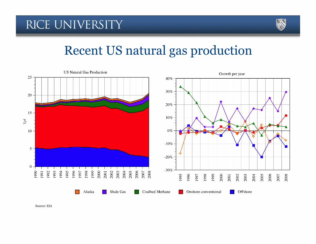
Recent US natural gas production

Source: EIA

Conventional versus Unconventional

!  Conventional reservoirs contain gas under pressure in interconnected pore spaces allowing flow to the wellbore

!  Unconventional reservoirs have low permeability, which must be enhanced to produce flow to the wellbore !  Tight Gas: Gas is sourced outside and migrates into the reservoir

!  CBM (or CSM): Coal seams act as source and reservoir of natural gas

!  Shale: Gas is sourced and trapped in a low permeability shale, which is usually either a source or a saturated cap spanning a large area

!  Hydraulic fracturing is a preferred method of stimulation !  Shale well water requirements (3-6 million gallons per well)

!  Some shales (e.g. Eagle Ford) have liquid-rich strata

Shale gas

!  Production from shale resembles a “just in time” manufacturing process !  Geologic uncertainty is lower

!  Fracing and production can be timed to maximize expected return

!  Initial production rates, and well productivity more generally, are growing due to innovations !  Examples include:

!  longer laterals: in Woodford, increased from 5 stages covering 2600 feet to 14 stages covering 6500 feet in the last 4 years

!  Multi-well pads !  Improved fracing fluids

Environmental concerns 1

!  Halliburton performed the first commercial “frac” in 1949 – it’s not new !  For shale gas, fracing regions are very deep – way below the water table

!  Fracing fluid is primarily water and sand or ceramics !  However, chemicals, some of which are toxic, are used to improve performance

!  While some fracing fluid chemicals remain in the shale, the majority of the fluid returns through the wellbore

!  Preventable problems can arise in the disposal process

!  Casing failures can also lead to contamination of near surface layers

!  CBM fracing can be more problematic than shale fracing because the coal is often closer to the surface (and can coincide with water aquifers)

!  CBM production also involves de-watering the coal to release the methane and this by-product needs treatment before being released

!  In some cases, however, treated water can be beneficial, for example for stock

Environmental concerns 2

!  In 2004 the US EPA found no evidence of contamination of drinking water from fracing

!  It nevertheless entered into a memorandum of agreement with CBM developers that precludes the use of diesel fuel in fracing fluids

!  The US EPA’s Underground Injection Control Program regulates !  Injection of fluids (Class II wells) to enhance oil and gas production

!  Fracturing used in connection with Class II and Class V injection wells to “stimulate” (open pore space in a formation)

!  Hydraulic fracturing to produce CBM in Alabama

!  The EPA Office of Research and Development is conducting a scientific study “to identify potential risks associated with Hydraulic Fracturing” and especially “the possible relationships between hydraulic fracturing and drinking water”

!  The state of New York announced a moratorium on hydraulic fracturing until the EPA study is completed

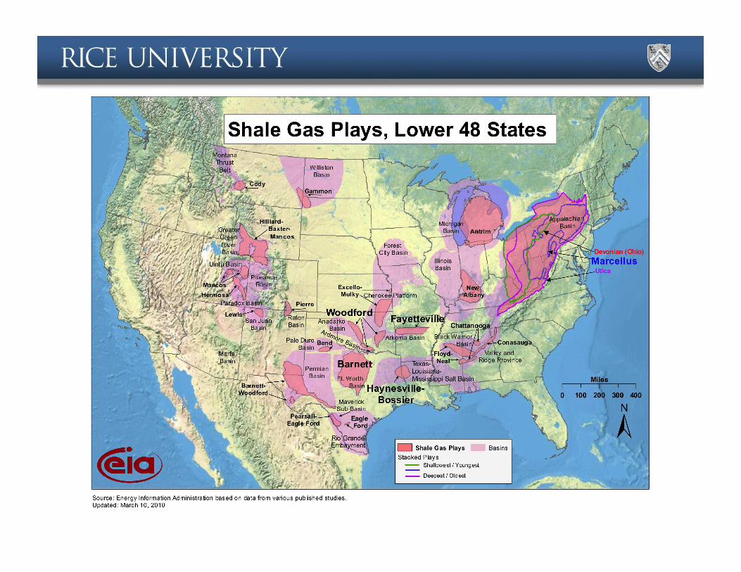
Shale is not confined to North America, and it has significant implications for the global gas market

Major North American Shale

Plays

European and Pacific Shale Plays

(Limited data available publicly)

North American Shale Gas

!  In 2005, most estimates placed the resource at about 140 tcf

!  The current resource assessment is large

!  The Rice model includes technically recoverable resources of 583 tcf

!  Some estimates are much higher

!  Navigant Consulting, Inc. (2008) estimated a mean of about 520 tcf

!  Potential Gas Committee (2009) over 680 tcf

!  Advanced Resources International estimate (2010) over 1000 tcf

The Global Shale Gas Resource

!  Rogner (1997) estimated over 16,000 tcf of shale gas resource in-place globally !  3842 North America

3528 China and India 2548 MENA 2313 Australasia 2117 Latin America 627 Former USSR 549 Europe 588 Other

!  Less that 10% was deemed technically recoverable and even less economically recoverable at current costs and prices

!  Only recently have innovations made this resource accessible

!  IEA recently estimated about 40% of the estimated resource in-place by Rogner (1997) will ultimately be technically recoverable

“Resource” vs. “Reserve” !  It is important to understand what these assessments are actually estimating

!  With shale gas, gas-in-place numbers are very large but the amount that is recoverable varies and depends costs and natural gas prices

Resource in Place

Resource endowment. Lots of uncertainty, but we can never get beyond this ultimate number.

Technically Recoverable Resource

This is the number that is being assessed. Lots of uncertainty, but experience has shown this number generally grows over time.

Economically Recoverable Resource

This will grow with decreasing costs and rising prices, but is bound by technology.

Proved Reserves

Connected and ready to produce.

Global shale gas resources in the Rice model

Country Basin/Region Mean Technically recoverable resource (tcf)

Austria Mikulov 30

Germany Lower Saxony 20

Poland Silurian 40

Sweden Alum 20

China South Central 30

Australia Cooper 40

The Rice World Gas Trade Model

The RWGTM

!  The Rice World Gas Trade Model (RWGTM) was developed to examine potential impacts of geopolitical, technological and other influences on the development of a global natural gas market

!  The model predicts regional prices, regional supplies and demands and inter-regional flows

!  Regions are defined at the country and sub-country level, with extensive representation of transportation infrastructure

!  The model is non-stochastic, but allows analysis of many different scenarios, including political actions that can trump economic outcomes

!  The model is constructed using the MarketBuilder software from Altos

!  Dynamic spatial general equilibrium linked through time by Hotelling-type optimization of resource extraction

!  Capacity expansion is determined by current and future prices along with capital costs of expansion, operating and maintenance costs of new and existing capacity, and revenues resulting from future outputs and prices.

The RWGTM: Demand •  Over 290 regions.

–  North America (residential, commercial, power generation and industrial sectors)

•  Natural gas demand functions estimated using longitudinal state and provincial data

–  Rest of World (Power Gen, Direct Use, EOR) •  Natural gas share of total energy increases with income, reflecting natural gas as a

premium fuel, but declines as relative price increases. The price elasticity is decreasing in the natural gas share of TPES. This captures rigidities associated with capital deployment.

•  Population growth taken from the UN median case projection to 2050

•  Economic growth is based on IMF forecasts and then a conditional growth convergence model

The RWGTM: Demand (cont.) !  Current economic and financial crisis is incorporated. We use the IMF outlook for growth

through 2014 for all countries. Beyond 2014, growth is governed by a model of conditional convergence. All GDP is in $2005PPP.

The RWGTM: Supply

!  Over 120 regions

!  Natural gas resources are represented as…

!  Conventional, CBM and shale in North America, China, Europe and Australia, and conventional gas deposits in the rest of the world

!  … in three categories

!  proved reserves (updated 2006 Oil & Gas Journal estimates)

!  growth in known reserves (P-50 USGS estimates and NPC estimates)

!  undiscovered resource (P-50 USGS estimates and NPC estimates)

!  North American cost-of-supply estimates were econometrically related to play-level geological characteristics and applied globally to generate costs for all regions of the world

!  Long run costs increase with depletion.

!  Short run adjustment costs limit the “rush to drill” phenomenon

!  We allow technological change to reduce mining costs longer term

Alternative technologies

!  In regions with substantial coal, we allow electricity generation demand to be lost to IGCC at a gas price of $6/mmbtu from 2010 !  However, IGCC is not much used before 2025

!  We also allow for unspecified new technologies to displace natural gas demand from 2020 at a price of $7/mmcf !  The unspecified backstop is not much used until after 2035

!  Work is in progress trying to better understand how alternative technologies may develop to displace natural gas demand

The RWGTM: Infrastructure

!  Required return on investment varies by region and type of project (using ICRG and World Bank data)

!  Detailed transportation network !  Pipelines are aggregated into corridors where appropriate, with the model choosing

utilization levels for current capacity and new pipeline links when profitable

!  Capital costs are based on an analysis of over 100 pipeline projects relating project cost to various factors

!  Tariffs are based on posted data, where available, and rate-of-return recovery

!  LNG is represented as a hub-and-spoke network, reflecting the assumption that capacity swaps will occur when profitable

!  LNG shipping rates based on lease rates and voyage time

!  For detailed information please see Peter Hartley and Kenneth B Medlock III, “The Baker Institute World Gas Trade Model” in The Geopolitics of Natural Gas, ed. Jaffe, Amy, David Victor and Mark Hayes, Cambridge University Press (2006)

Base case results

Base case results: Demand

Base case results: Supply

Base case results: North America wellhead supply

Base case results: European wellhead supply

Base case results: Trade

Base case results: LNG exports

Base case results: LNG imports

Base case results: Singapore flows

Base case results: Singapore regional LNG trades

Base case results: Select prices

Effects of excluding new shale production

Changes in North America wellhead supply

Changes in European wellhead supply

Changes in select prices

Overall supply changes

Demand changes

Increase in demand lost to alternatives

Changes in imports

Changes in exports

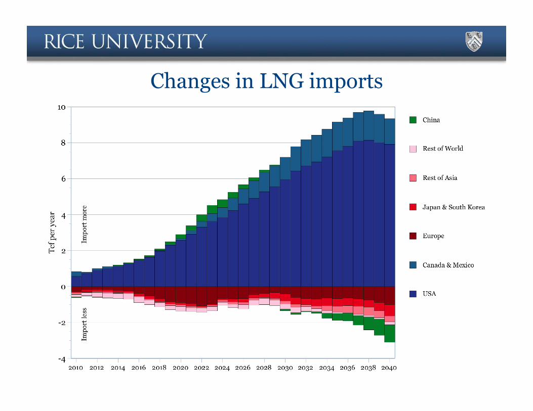
Changes in LNG imports

Changes in LNG exports

Concluding Remarks – Reference case !  As a premium fuel, natural gas demand generally grows faster than output

!  Asia is the largest source of growing demand

!  Gas prices steadily rise as a result of depletion and, around 2035 in our simulations, other energy sources become competitive and dampen gas demand growth

!  Supply growth is fastest in the Middle East and, to a lesser extent, Russia

!  LNG trade links prices around the world – the size of a link does not affect the possibility of arbitrage, only the speed of price adjustments

!  By 2036, LNG accounts for over 50% of all internationally traded natural gas

!  LNG exports grow fastest in the Middle East and Australia

!  LNG imports grow most in Europe & Asia; US regas terminal load factors remain low through the 2020s

!  Basis differentials largely reflect transportation costs, although lumpiness in investments can also play a role

!  Singapore is a hub of flows from several directions, with substantial LNG flows in the vicinity, making it a possible LNG price-setting focal point and natural gas trading center if it can encourage standardized contracts with transparent prices

Concluding Remarks – Consequences of shale

!  Likely development of US and Canadian shale gas resources, especially beyond 2015, limits the growth of LNG imports into the US

!  Nevertheless, declines in production from other sources eventually stimulate substantial growth in US LNG imports beyond 2025

!  If shale is not developed as forecast, for example for environmental reasons, North American LNG imports would be dramatically higher

!  Reduced shale gas would directly affect the Atlantic Basin LNG market, but trade would spread higher prices around the world, dampening demand in most places

!  Higher prices would also stimulate alternative supply, especially from Russia and the Middle East, but aggregate supply nevertheless would fall

!  Small reductions in imports, especially in Asia, would liberate some LNG to satisfy increased demand from North America

!  A small shift in European supply toward pipeline gas would also free some LNG for North America

!  A lack of shale development also would stimulate backstop demand