Potential slab avalanche release area identiﬁcation from ... · Received: 8 September 2015 ... which cause the vast majority of ... the fuzzy logic approach in an effort to deal

Nat. Hazards Earth Syst. Sci., 16, 2211–2225, 2016www.nat-hazards-earth-syst-sci.net/16/2211/2016/doi:10.5194/nhess-16-2211-2016© Author(s) 2016. CC Attribution 3.0 License.

Potential slab avalanche release area identification from estimatedwinter terrain: a multi-scale, fuzzy logic approachJochen Veitinger1, Ross Stuart Purves2, and Betty Sovilla1

1WSL Institute for Snow and Avalanche Research SLF, Davos, Switzerland2Department of Geography, University of Zurich, Zurich, Switzerland

Correspondence to: Jochen Veitinger ([email protected])

Received: 8 September 2015 – Published in Nat. Hazards Earth Syst. Sci. Discuss.: 29 October 2015Revised: 13 July 2016 – Accepted: 25 August 2016 – Published: 7 October 2016

Abstract. Avalanche hazard assessment requires a very pre-cise estimation of the release area, which still depends, toa large extent, on expert judgement of avalanche special-ists. Therefore, a new algorithm for automated identificationof potential avalanche release areas was developed. It over-comes some of the limitations of previous tools, which arecurrently not often applied in hazard mitigation practice. Byintroducing a multi-scale roughness parameter, fine-scale to-pography and its attenuation under snow influence is cap-tured. This allows the assessment of snow influence on ter-rain morphology and, consequently, potential release areasize and location. The integration of a wind shelter index en-ables the user to define release area scenarios as a function ofthe prevailing wind direction or single storm events. A casestudy illustrates the practical usefulness of this approach forthe definition of release area scenarios under varying snowcover and wind conditions. A validation with historical datademonstrated an improved estimation of avalanche releaseareas. Our method outperforms a slope-based approach, inparticular for more frequent avalanches; however, the appli-cation of the algorithm as a forecasting tool remains limited,as snowpack stability is not integrated. Future research activ-ity should therefore focus on the coupling of the algorithmwith snowpack conditions.

1 Introduction

Location and extent of avalanche starting zones are of cru-cial importance in order to correctly estimate the potentialdanger that avalanches pose to roads, railways and other in-frastructure. In current engineering practice for hazard map-

ping and planning of long-term mitigation measures, releasearea size is a key input in numerical models of avalanche dy-namics such as RAMMS (Christen et al., 2010) or SAMOS-AT (Sampl and Granig, 2009; Sampl and Zwinger, 2004).They allow the assessment of run-out, velocity, flow heightor impact pressure of avalanches, and are especially impor-tant when historical data are sparse or completely lacking.Studies of modelling extreme (Barbolini et al., 2000), as wellas small and frequent avalanches (Dreier et al., 2014), haverevealed high model sensitivity to changes of release areasize and location. Therefore, a very precise definition of po-tential release areas is not only crucial for hazard mappingor long-term mitigation purposes, but is a precondition forsuccessful integration of avalanche dynamics simulations inthe planning of more short-term mitigation measures, such asroad closures or ski resort safety, where small and frequentavalanches also pose a threat.

1.1 Modelling potential release areas

The complex task of release area estimation remains subjectto the individual judgement of avalanche experts. It is basedon terrain analysis, historical data, field visits and, for exam-ple, aerial photography of the winter surface. Nonetheless,with increasing availability of geographic information sys-tems (GISs) and digital terrain models (DEMs), the devel-opment of algorithms centred on automating the process ofrelease area definition has been attempted. Such algorithmsare mainly based on terrain parameters, such as slope, aspectand curvature derived from digital terrain models (DTMs)(Maggioni and Gruber, 2003; Bühler et al., 2012). Some au-thors use additional snow meteorological parameters such asthe duration of snow cover (Pistocchi and Notarnicola, 2013)

Published by Copernicus Publications on behalf of the European Geosciences Union.

2212 J. Veitinger et al.: Slab avalanche release area estimation

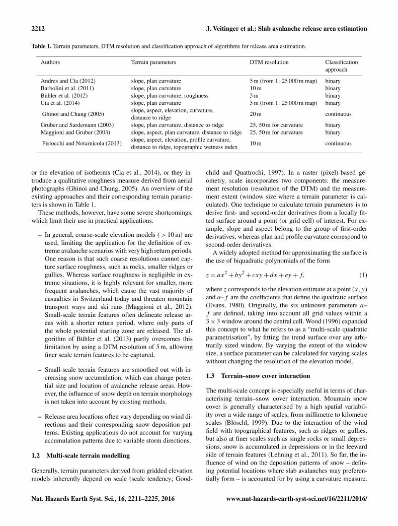
Table 1. Terrain parameters, DTM resolution and classification approach of algorithms for release area estimation.

Authors Terrain parameters DTM resolution Classificationapproach

Andres and Cía (2012) slope, plan curvature 5 m (from 1 : 25 000 m map) binaryBarbolini et al. (2011) slope, plan curvature 10 m binaryBühler et al. (2012) slope, plan curvature, roughness 5 m binaryCia et al. (2014) slope, plan curvature 5 m (from 1 : 25 000 m map) binary

Ghinoi and Chung (2005)slope, aspect, elevation, curvature,

20 m continuousdistance to ridge

Gruber and Sardemann (2003) slope, plan curvature, distance to ridge 25, 50 m for curvature binaryMaggioni and Gruber (2003) slope, aspect, plan curvature, distance to ridge 25, 50 m for curvature binary

Pistocchi and Notarnicola (2013)slope, aspect, elevation, profile curvature,

10 m continuousdistance to ridge, topographic wetness index

or the elevation of isotherms (Cia et al., 2014), or they in-troduce a qualitative roughness measure derived from aerialphotographs (Ghinoi and Chung, 2005). An overview of theexisting approaches and their corresponding terrain parame-ters is shown in Table 1.

These methods, however, have some severe shortcomings,which limit their use in practical applications.

– In general, coarse-scale elevation models (> 10 m) areused, limiting the application for the definition of ex-treme avalanche scenarios with very high return periods.One reason is that such coarse resolutions cannot cap-ture surface roughness, such as rocks, smaller ridges orgullies. Whereas surface roughness is negligible in ex-treme situations, it is highly relevant for smaller, morefrequent avalanches, which cause the vast majority ofcasualties in Switzerland today and threaten mountaintransport ways and ski runs (Maggioni et al., 2012).Small-scale terrain features often delineate release ar-eas with a shorter return period, where only parts ofthe whole potential starting zone are released. The al-gorithm of Bühler et al. (2013) partly overcomes thislimitation by using a DTM resolution of 5 m, allowingfiner scale terrain features to be captured.

– Small-scale terrain features are smoothed out with in-creasing snow accumulation, which can change poten-tial size and location of avalanche release areas. How-ever, the influence of snow depth on terrain morphologyis not taken into account by existing methods.

– Release area locations often vary depending on wind di-rections and their corresponding snow deposition pat-terns. Existing applications do not account for varyingaccumulation patterns due to variable storm directions.

1.2 Multi-scale terrain modelling

Generally, terrain parameters derived from gridded elevationmodels inherently depend on scale (scale tendency; Good-

child and Quattrochi, 1997). In a raster (pixel)-based ge-ometry, scale incorporates two components: the measure-ment resolution (resolution of the DTM) and the measure-ment extent (window size where a terrain parameter is cal-culated). One technique to calculate terrain parameters is toderive first- and second-order derivatives from a locally fit-ted surface around a point (or grid cell) of interest. For ex-ample, slope and aspect belong to the group of first-orderderivatives, whereas plan and profile curvature correspond tosecond-order derivatives.

A widely adopted method for approximating the surface isthe use of biquadratic polynomials of the form

z= ax2+ by2

+ cxy+ dx+ ey+ f, (1)

where z corresponds to the elevation estimate at a point (x, y)and a–f are the coefficients that define the quadratic surface(Evans, 1980). Originally, the six unknown parameters a–f are defined, taking into account all grid values within a3× 3 window around the central cell. Wood (1996) expandedthis concept to what he refers to as a “multi-scale quadraticparametrisation”, by fitting the trend surface over any arbi-trarily sized window. By varying the extent of the windowsize, a surface parameter can be calculated for varying scaleswithout changing the resolution of the elevation model.

1.3 Terrain–snow cover interaction

The multi-scale concept is especially useful in terms of char-acterising terrain–snow cover interaction. Mountain snowcover is generally characterised by a high spatial variabil-ity over a wide range of scales, from millimetre to kilometrescales (Blöschl, 1999). Due to the interaction of the windfield with topographical features, such as ridges or gullies,but also at finer scales such as single rocks or small depres-sions, snow is accumulated in depressions or in the leewardside of terrain features (Lehning et al., 2011). So far, the in-fluence of wind on the deposition patterns of snow – defin-ing potential locations where slab avalanches may preferen-tially form – is accounted for by using a curvature measure.

Nat. Hazards Earth Syst. Sci., 16, 2211–2225, 2016 www.nat-hazards-earth-syst-sci.net/16/2211/2016/

J. Veitinger et al.: Slab avalanche release area estimation 2213

A parameter capturing the exposure and sheltering effects ofterrain relative to a given wind direction could be, however,very beneficial to formulating release area scenarios. Terrain-based parameters with the aim of capturing wind shelter andexposure have been developed in the past (Winstral et al.,2002; Purves et al., 1998) and have been shown to capturewind sheltering effects and realistically produce accumula-tion patterns of snow (Schirmer et al., 2011; Erickson et al.,2005). They could hence easily be integrated into release areaestimation procedures.

Another result of irregular snow accumulation is a pro-gressive cancelling out of surface roughness, leading toincreasingly homogeneous snow deposition patterns (Mottet al., 2010). It is assumed that this may lead to a moreuniform slab thickness and, in combination with reducedsupport from the bed surface, to potentially larger releasearea sizes – in particular for surface slabs (McClung, 2001;Simenhois and Birkeland, 2008). Further, Veitinger et al.(2014) showed that the progressive smoothing of surfaceroughness can be captured by a multi-scale roughness pa-rameter. So far, roughness is only incorporated in some ap-proaches as a single-scale terrain parameter, often not reflect-ing the adequate scale of a given snow scenario.

1.4 Fuzzy logic modelling for natural hazards

Natural processes can rarely be described or modelled as aresult of sharply defined criteria or variables. Expert deci-sion making therefore contains significant degrees of uncer-tainty owing to the complex nature of the process and theparameters involved. Current algorithms often do not con-sider this uncertainty in input parameters as they incorporatebinary classification schemes, where the result strongly de-pends on the definition of thresholds. As a result, such algo-rithms can only distinguish between areas where avalanchesare possible and where they are not. Consequently, existingrelease area algorithms mainly produce worst case scenar-ios, including all possible areas that can potentially releaseavalanches. Whilst this may be appropriate for an extremesituation, it is not suited to delineate smaller release areas,where only parts of the potential area release avalanches.Such issues cannot be solved through a classical logic ap-proach; therefore, with this in mind, Zadeh (1965) introducedthe fuzzy logic approach in an effort to deal with such im-precise data or diffuse rules. This approach overcomes theconcept of sharp (so-called crisp) borders by introducing themembership concept. Every element, as opposed to belong-ing (or not) to a class, is attributed a degree of membershipbelonging to that class (referred to as a set in fuzzy set the-ory). This concept is very appealing for natural hazards ap-plications as it allows the integration of human reasoning ca-pabilities into knowledge–based expert systems. Moreover, ithas already been successfully applied to landslide suscepti-bility mapping (Schernthanner, 2007), risk modelling of wetsnow avalanches (Zischg et al., 2005) and avalanche release

area estimation (Ghinoi and Chung, 2005). Such an approachwould be particularly helpful for the definition of more fre-quent avalanches, where a differentiation between areas ofdifferent likelihoods of releasing avalanches is necessary.

Therefore, in this paper we present a new algorithm to de-fine potential release areas, which improves on existing ap-proaches by taking into account the effects of snow coverand wind transport on the summer terrain. Specifically, weintroduce a multi-scale roughness parameter, where scale isadjusted as a function of snow depth, and we include a windshelter index to define release area scenarios as a function ofvarying snow accumulation due to wind. This allows calcu-lation of potential release area size with a snow-distribution-dependent parameter. By using fuzzy logic to combine infor-mation we can further distinguish between different gradesof release propensity. Thus, our approach allows for a defi-nition of potential release areas, which goes beyond purelyterrain-based parameters. Such approaches are particularlyimportant for frequent avalanches and avalanche dynamicssimulations of short-term hazard, for example in the case ofroad closures.

2 Methods

2.1 Overview

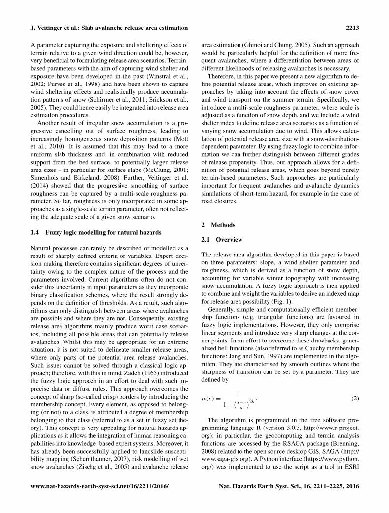
The release area algorithm developed in this paper is basedon three parameters: slope, a wind shelter parameter androughness, which is derived as a function of snow depth,accounting for variable winter topography with increasingsnow accumulation. A fuzzy logic approach is then appliedto combine and weight the variables to derive an indexed mapfor release area possibility (Fig. 1).

Generally, simple and computationally efficient member-ship functions (e.g. triangular functions) are favoured infuzzy logic implementations. However, they only compriselinear segments and introduce very sharp changes at the cor-ner points. In an effort to overcome these drawbacks, gener-alised bell functions (also referred to as Cauchy membershipfunctions; Jang and Sun, 1997) are implemented in the algo-rithm. They are characterised by smooth outlines where thesharpness of transition can be set by a parameter. They aredefined by

µ(x)=1

1+(x−ca

)2b . (2)

The algorithm is programmed in the free software pro-gramming language R (version 3.0.3, http://www.r-project.org); in particular, the geocomputing and terrain analysisfunctions are accessed by the RSAGA package (Brenning,2008) related to the open source desktop GIS, SAGA (http://www.saga-gis.org). A Python interface (https://www.python.org/) was implemented to use the script as a tool in ESRI

www.nat-hazards-earth-syst-sci.net/16/2211/2016/ Nat. Hazards Earth Syst. Sci., 16, 2211–2225, 2016

http://www.r-project.org

http://www.r-project.org

http://www.saga-gis.org

http://www.saga-gis.org

https://www.python.org/

https://www.python.org/


ArcGIS (ArcGIS 10.2 for Desktop). The model code of therelease area algorithm can be found in Veitinger et al. (2016).

In the next sections, the choice of the parameters, as wellas the selection of value ranges to define the membershipfunctions, is explained.

2.2 Parameter derivation

2.2.1 Slope

One of the most relevant terrain variables for the defini-tion of avalanche starting zones is slope. Slope maps areregularly consulted in current avalanche hazard mappingpractice as a basis for release area assessment. Generally,slab avalanches are released on slopes between 28 and 55◦

(Perla, 1977; Schweizer and Lütschg, 2001; Schweizer andJamieson, 2001). An increased release probability is gener-ally observed above 35◦ (Stoffel and Margreth, 2012). Withrespect to size, avalanches occurring below 35◦ are oftenlarge. For very steep regions (> 45◦), release probability forlarge avalanches decreases because of constant sluffing andavalanching, which prevent the formation of a continuousweak layer. Mostly small, frequent avalanches are observed.Above 55◦, sluffing hinders the formation of slabs (McClungand Schaerer, 2002), and only loose snow avalanches orsluffs are observed.

To calculate slope using quadratic parametrisation as pro-posed by Wood (1996), the magnitude (slope) of the steepestgradient at the central grid cell of the fitted surface needs tobe determined. To derive this, the rate of change in x andy direction is calculated as follows:

dzdxy=

√( dzdx

)2

+

(dzdy

)2 . (3)

The partial derivatives for x and y are noted as

dzdx= 2ax+ cy+ d, (4)

anddzdy= 2by+ cx+ e. (5)

In order to obtain the parameter at the central point ofthe surface (x= y= 0), Eqs. (4) and (5) are integrated intoEq. (3), and note

dzdxy=

√d2+ e2. (6)

Slope (α) is thus given as

α = arctan√d2+ e2. (7)

Likewise, aspect is defined as

β = arctane

d. (8)

The aforementioned definitions are consistent with others,as reported in the literature (Zevenbergen and Thorne, 1987).Based on multi-scale slope and aspect, several other terrainparameters such as roughness and wind shelter can be de-rived (see following sections).

In our algorithm, slope values between 28 and 60◦ are con-sidered to be potential release areas. The degree of member-ship µs(x) to the class PRA of slope is modelled using a gen-eralised bell membership function with the parameters a= 8,b= 3 and c= 40 (Fig. 2).

This function assigns the largest membership degrees toslopes of between 35 and 45◦. Slopes less steep than 30◦

and steeper than 55◦ are assigned low membership degreesas slab avalanches become increasingly unlikely for suchslopes.

2.2.2 Wind shelter

Wind–terrain interaction is often mentioned in literature asan important factor to explain the location of slab avalanches.Concave areas are generally considered to be more prone toavalanche release than convex terrain (Maggioni and Gruber,2003; Vontobel, 2011). One possible reason is that snow un-der wind influence is irregularly distributed and deposited,favouring leeward slopes, gullies or downslope terrain steep-ening. At a slope scale, wind drift (Gauer, 2001) and pref-erential deposition of precipitation (Lehning et al., 2008)are the main influencing processes for snow redistribution.Based on the importance of wind–terrain interaction for snowdistribution, we consider a wind shelter parameter to be supe-rior compared to a regular curvature measure for two reasons.

1. A wind shelter parameter accounts for sheltering ef-fects independent of the direction (downslope or across-slope) of a curvature measure.

2. Sheltering effects can be derived as a function of winddirection. This allows refined calculations, taking intoaccount local particularities such as the main wind di-rection.

In this study, the wind shelter parameter of Plattner et al.(2006) is utilised, based on the wind sheltering parameter ofWinstral et al. (2002) of the form

index(S)= arctanmax(z (x0)− z(x))

|x0− x|: x ∈ S, (9)

where S= S(x0, a, δa, d) is a subset of grid cells within adistance of δd and a range of direction of a± δa from thecentral cell x0. In our implementation we replaced the MAXfunction by the quantile function using the third quantile in-stead of the MAX. This accounts for the fact that locally,very large sheltering effects might be outweighed if the sur-rounding area is open to wind influence (e.g. large rocks inan otherwise open slope). The wind shelter index varies be-tween−1.5 and 1.5 for complex alpine terrain. Negative val-ues correspond to wind-exposed terrain, and positive values



Snow depth

Wind direction + tolerance

DTM (2m resolution)

Roughness

Slope

Wind shelter

Map ofpotential

release areas

Resamplingto 10 m +

slopecomputation

computation

Fuzzy logicoperator

Optional forestmask

Multi-scaleroughness

computation

Wind shelter

Figure 1. Schematic overview of the release area algorithm showing the input data (blue), processing steps (yellow) and output raster data(green).

Figure 2. Fuzzy membership function for slope.

to wind-sheltered terrain; therefore, the degree of member-ship µw(x) to the class PRA of wind shelter is modelled us-ing a generalised bell membership function with the param-eters a= 2, b= 3 and c= 2 (Fig. 3).

2.2.3 Roughness

Surface roughness was mentioned as early as 1959, dur-ing which time it was recognised as an important parameterfor avalanche release (Peev, 1959). In a shallow snowpack,terrain roughness can have a stabilising function, hinderingthe formation of continuous weak layers (Schweizer et al.,2003), as well as providing mechanical support to the snow-pack (McClung, 2001). However, increasing snow accumu-lation is known to smooth out surface roughness (Veitingeret al., 2014), reducing snowpack variability in the surfacelayers (Mott et al., 2010) and the mechanical support of aslab (van Herwijnen and Heierli, 2009). In this case, the sta-bilising effects of terrain roughness disappear or even reverse(McClung and Schaerer, 2002), and the formation of contin-uous weak layers and slabs, which favours fracture propa-gation (Simenhois and Birkeland, 2008), is facilitated. Thisaffects potential release area size and location – especially inthe case of surface slab avalanches. Therefore, it seems crit-

Figure 3. Fuzzy membership function for wind shelter.

ical to consider roughness together with its alteration due tosnow accumulation.

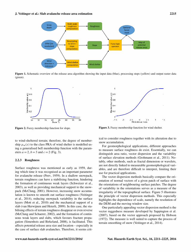
For geomorphological applications, different approachesto measure surface roughness do exist. Essentially, we candistinguish area ratio, vector dispersion and the variabilityof surface elevation methods (Grohmann et al., 2011). No-tably, other methods, such as fractal dimension or wavelets,are not directly linked to measurable geomorphological vari-ables, and are therefore difficult to interpret, limiting theiruse for practical applications.

The vector dispersion methods basically compare the ori-entation of normal vectors of a given patch of surface withthe orientations of neighbouring surface patches. The degreeof variability in the orientations serves as a measure of theirregularity of the topographical surface. Figure 5 illustratesthe principle of vector dispersion methods. This especiallyhighlights the dependence of scale, namely the resolution ofthe DEM and the moving window size.

One particularly appealing vector dispersion method is thevector ruggedness measure developed by Sappington et al.(2007), based on the vector approach proposed by Hobson(1972). The measure is well suited to capture the process ofterrain smoothing of snow (Veitinger et al., 2014).



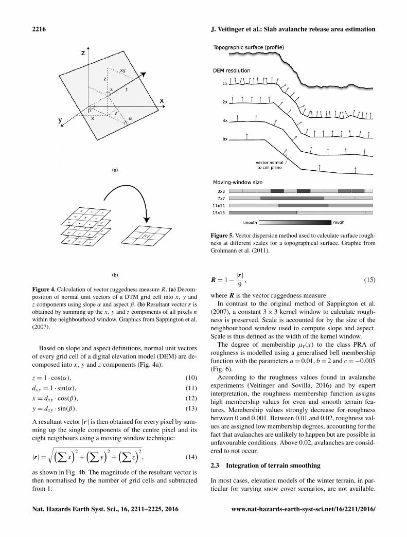
Figure 4. Calculation of vector ruggedness measure R. (a) Decom-position of normal unit vectors of a DTM grid cell into x, y andz components using slope α and aspect β. (b) Resultant vector r isobtained by summing up the x, y and z components of all pixels nwithin the neighbourhood window. Graphics from Sappington et al.(2007).

Based on slope and aspect definitions, normal unit vectorsof every grid cell of a digital elevation model (DEM) are de-composed into x, y and z components (Fig. 4a):

z= 1 · cos(α), (10)dxy = 1 · sin(α), (11)x = dxy · cos(β), (12)y = dxy · sin(β). (13)

A resultant vector |r| is then obtained for every pixel by sum-ming up the single components of the centre pixel and itseight neighbours using a moving window technique:

|r| =

√(∑x)2+

(∑y)2+

(∑z)2, (14)

as shown in Fig. 4b. The magnitude of the resultant vector isthen normalised by the number of grid cells and subtractedfrom 1:

Figure 5. Vector dispersion method used to calculate surface rough-ness at different scales for a topographical surface. Graphic fromGrohmann et al. (2011).

R = 1−|r|

9, (15)

where R is the vector ruggedness measure.In contrast to the original method of Sappington et al.

(2007), a constant 3× 3 kernel window to calculate rough-ness is preserved. Scale is accounted for by the size of theneighbourhood window used to compute slope and aspect.Scale is thus defined as the width of the kernel window.

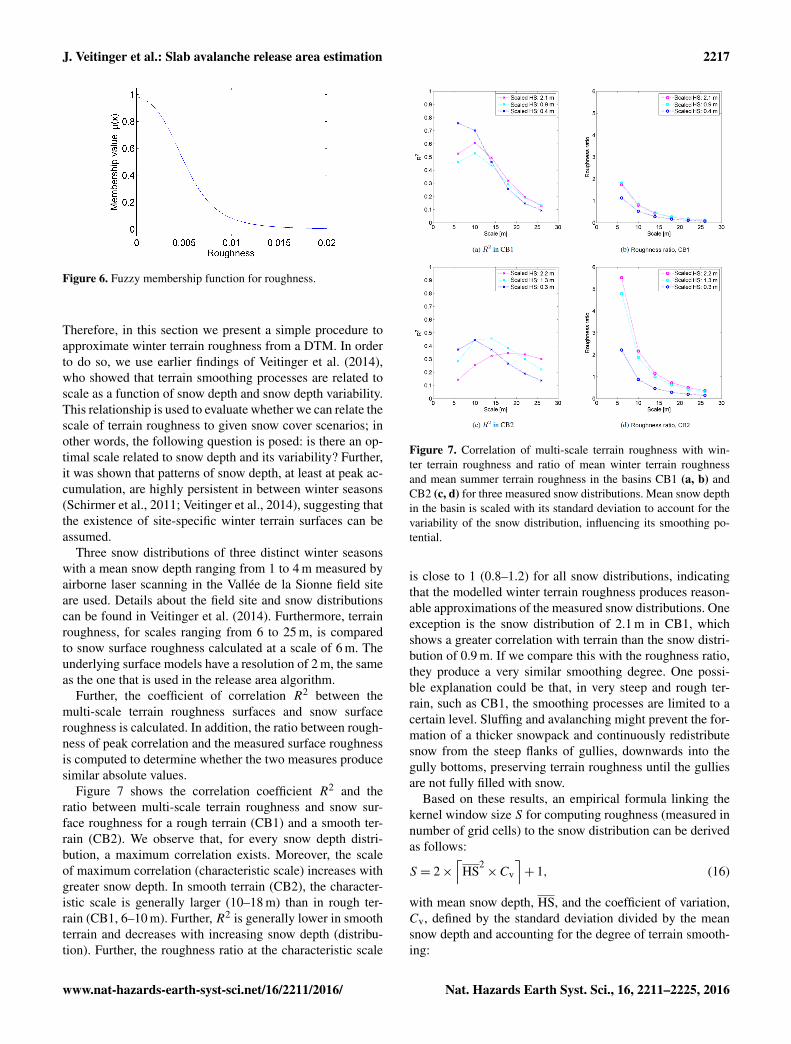
The degree of membership µr(x) to the class PRA ofroughness is modelled using a generalised bell membershipfunction with the parameters a= 0.01, b= 2 and c=−0.005(Fig. 6).

According to the roughness values found in avalancheexperiments (Veitinger and Sovilla, 2016) and by expertinterpretation, the roughness membership function assignshigh membership values for even and smooth terrain fea-tures. Membership values strongly decrease for roughnessbetween 0 and 0.001. Between 0.01 and 0.02, roughness val-ues are assigned low membership degrees, accounting for thefact that avalanches are unlikely to happen but are possible inunfavourable conditions. Above 0.02, avalanches are consid-ered to not occur.

2.3 Integration of terrain smoothing

In most cases, elevation models of the winter terrain, in par-ticular for varying snow cover scenarios, are not available.



Figure 6. Fuzzy membership function for roughness.

Therefore, in this section we present a simple procedure toapproximate winter terrain roughness from a DTM. In orderto do so, we use earlier findings of Veitinger et al. (2014),who showed that terrain smoothing processes are related toscale as a function of snow depth and snow depth variability.This relationship is used to evaluate whether we can relate thescale of terrain roughness to given snow cover scenarios; inother words, the following question is posed: is there an op-timal scale related to snow depth and its variability? Further,it was shown that patterns of snow depth, at least at peak ac-cumulation, are highly persistent in between winter seasons(Schirmer et al., 2011; Veitinger et al., 2014), suggesting thatthe existence of site-specific winter terrain surfaces can beassumed.

Three snow distributions of three distinct winter seasonswith a mean snow depth ranging from 1 to 4 m measured byairborne laser scanning in the Vallée de la Sionne field siteare used. Details about the field site and snow distributionscan be found in Veitinger et al. (2014). Furthermore, terrainroughness, for scales ranging from 6 to 25 m, is comparedto snow surface roughness calculated at a scale of 6 m. Theunderlying surface models have a resolution of 2 m, the sameas the one that is used in the release area algorithm.

Further, the coefficient of correlation R2 between themulti-scale terrain roughness surfaces and snow surfaceroughness is calculated. In addition, the ratio between rough-ness of peak correlation and the measured surface roughnessis computed to determine whether the two measures producesimilar absolute values.

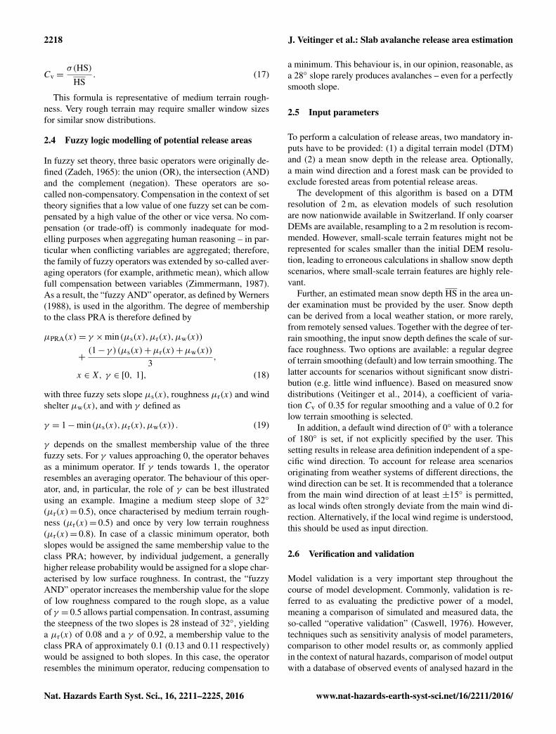
Figure 7 shows the correlation coefficient R2 and theratio between multi-scale terrain roughness and snow sur-face roughness for a rough terrain (CB1) and a smooth ter-rain (CB2). We observe that, for every snow depth distri-bution, a maximum correlation exists. Moreover, the scaleof maximum correlation (characteristic scale) increases withgreater snow depth. In smooth terrain (CB2), the character-istic scale is generally larger (10–18 m) than in rough ter-rain (CB1, 6–10 m). Further, R2 is generally lower in smoothterrain and decreases with increasing snow depth (distribu-tion). Further, the roughness ratio at the characteristic scale

Figure 7. Correlation of multi-scale terrain roughness with win-ter terrain roughness and ratio of mean winter terrain roughnessand mean summer terrain roughness in the basins CB1 (a, b) andCB2 (c, d) for three measured snow distributions. Mean snow depthin the basin is scaled with its standard deviation to account for thevariability of the snow distribution, influencing its smoothing po-tential.

is close to 1 (0.8–1.2) for all snow distributions, indicatingthat the modelled winter terrain roughness produces reason-able approximations of the measured snow distributions. Oneexception is the snow distribution of 2.1 m in CB1, whichshows a greater correlation with terrain than the snow distri-bution of 0.9 m. If we compare this with the roughness ratio,they produce a very similar smoothing degree. One possi-ble explanation could be that, in very steep and rough ter-rain, such as CB1, the smoothing processes are limited to acertain level. Sluffing and avalanching might prevent the for-mation of a thicker snowpack and continuously redistributesnow from the steep flanks of gullies, downwards into thegully bottoms, preserving terrain roughness until the gulliesare not fully filled with snow.

Based on these results, an empirical formula linking thekernel window size S for computing roughness (measured innumber of grid cells) to the snow distribution can be derivedas follows:

S = 2×⌈

HS2×Cv

⌉+ 1, (16)

with mean snow depth, HS, and the coefficient of variation,Cv, defined by the standard deviation divided by the meansnow depth and accounting for the degree of terrain smooth-ing:



Cv =σ(HS)

HS. (17)

This formula is representative of medium terrain rough-ness. Very rough terrain may require smaller window sizesfor similar snow distributions.

2.4 Fuzzy logic modelling of potential release areas

In fuzzy set theory, three basic operators were originally de-fined (Zadeh, 1965): the union (OR), the intersection (AND)and the complement (negation). These operators are so-called non-compensatory. Compensation in the context of settheory signifies that a low value of one fuzzy set can be com-pensated by a high value of the other or vice versa. No com-pensation (or trade-off) is commonly inadequate for mod-elling purposes when aggregating human reasoning – in par-ticular when conflicting variables are aggregated; therefore,the family of fuzzy operators was extended by so-called aver-aging operators (for example, arithmetic mean), which allowfull compensation between variables (Zimmermann, 1987).As a result, the “fuzzy AND” operator, as defined by Werners(1988), is used in the algorithm. The degree of membershipto the class PRA is therefore defined by

µPRA(x)= γ ×min(µs(x),µr(x),µw(x))

+(1− γ )(µs(x)+µr(x)+µw(x))

3,

x ∈X, γ ∈ [0, 1], (18)

with three fuzzy sets slope µs(x), roughness µr(x) and windshelter µw(x), and with γ defined as

γ = 1−min(µs(x),µr(x),µw(x)) . (19)

γ depends on the smallest membership value of the threefuzzy sets. For γ values approaching 0, the operator behavesas a minimum operator. If γ tends towards 1, the operatorresembles an averaging operator. The behaviour of this oper-ator, and, in particular, the role of γ can be best illustratedusing an example. Imagine a medium steep slope of 32◦

(µr(x)= 0.5), once characterised by medium terrain rough-ness (µr(x)= 0.5) and once by very low terrain roughness(µr(x)= 0.8). In case of a classic minimum operator, bothslopes would be assigned the same membership value to theclass PRA; however, by individual judgement, a generallyhigher release probability would be assigned for a slope char-acterised by low surface roughness. In contrast, the “fuzzyAND” operator increases the membership value for the slopeof low roughness compared to the rough slope, as a valueof γ = 0.5 allows partial compensation. In contrast, assumingthe steepness of the two slopes is 28 instead of 32◦, yieldinga µr(x) of 0.08 and a γ of 0.92, a membership value to theclass PRA of approximately 0.1 (0.13 and 0.11 respectively)would be assigned to both slopes. In this case, the operatorresembles the minimum operator, reducing compensation to

a minimum. This behaviour is, in our opinion, reasonable, asa 28◦ slope rarely produces avalanches – even for a perfectlysmooth slope.

2.5 Input parameters

To perform a calculation of release areas, two mandatory in-puts have to be provided: (1) a digital terrain model (DTM)and (2) a mean snow depth in the release area. Optionally,a main wind direction and a forest mask can be provided toexclude forested areas from potential release areas.

The development of this algorithm is based on a DTMresolution of 2 m, as elevation models of such resolutionare now nationwide available in Switzerland. If only coarserDEMs are available, resampling to a 2 m resolution is recom-mended. However, small-scale terrain features might not berepresented for scales smaller than the initial DEM resolu-tion, leading to erroneous calculations in shallow snow depthscenarios, where small-scale terrain features are highly rele-vant.

Further, an estimated mean snow depth HS in the area un-der examination must be provided by the user. Snow depthcan be derived from a local weather station, or more rarely,from remotely sensed values. Together with the degree of ter-rain smoothing, the input snow depth defines the scale of sur-face roughness. Two options are available: a regular degreeof terrain smoothing (default) and low terrain smoothing. Thelatter accounts for scenarios without significant snow distri-bution (e.g. little wind influence). Based on measured snowdistributions (Veitinger et al., 2014), a coefficient of varia-tion Cv of 0.35 for regular smoothing and a value of 0.2 forlow terrain smoothing is selected.

In addition, a default wind direction of 0◦ with a toleranceof 180◦ is set, if not explicitly specified by the user. Thissetting results in release area definition independent of a spe-cific wind direction. To account for release area scenariosoriginating from weather systems of different directions, thewind direction can be set. It is recommended that a tolerancefrom the main wind direction of at least ±15◦ is permitted,as local winds often strongly deviate from the main wind di-rection. Alternatively, if the local wind regime is understood,this should be used as input direction.

2.6 Verification and validation

Model validation is a very important step throughout thecourse of model development. Commonly, validation is re-ferred to as evaluating the predictive power of a model,meaning a comparison of simulated and measured data, theso-called “operative validation” (Caswell, 1976). However,techniques such as sensitivity analysis of model parameters,comparison to other model results or, as commonly appliedin the context of natural hazards, comparison of model outputwith a database of observed events of analysed hazard in the



past (event validation), can be considered proper validationtechniques (Rykiel Jr., 1996).

Further, in the case of a continuous model output, a divi-sion into several hazard classes is commonly requested bydecision makers for practical reasons (such as the planningof mitigation measures, for example). The selection of suchdecision thresholds depends on the context of application ofthe hazard model and the costs associated with the two errortypes (false positives/negatives) rather than on the character-istics of the model itself. Accordingly, in this vein, Beguería(2006) proposes the conduction of the model validation inde-pendently of various final thresholds, and to use such valida-tion output to propose decision thresholds, including associ-ated confidence measures for the end users of hazard models.

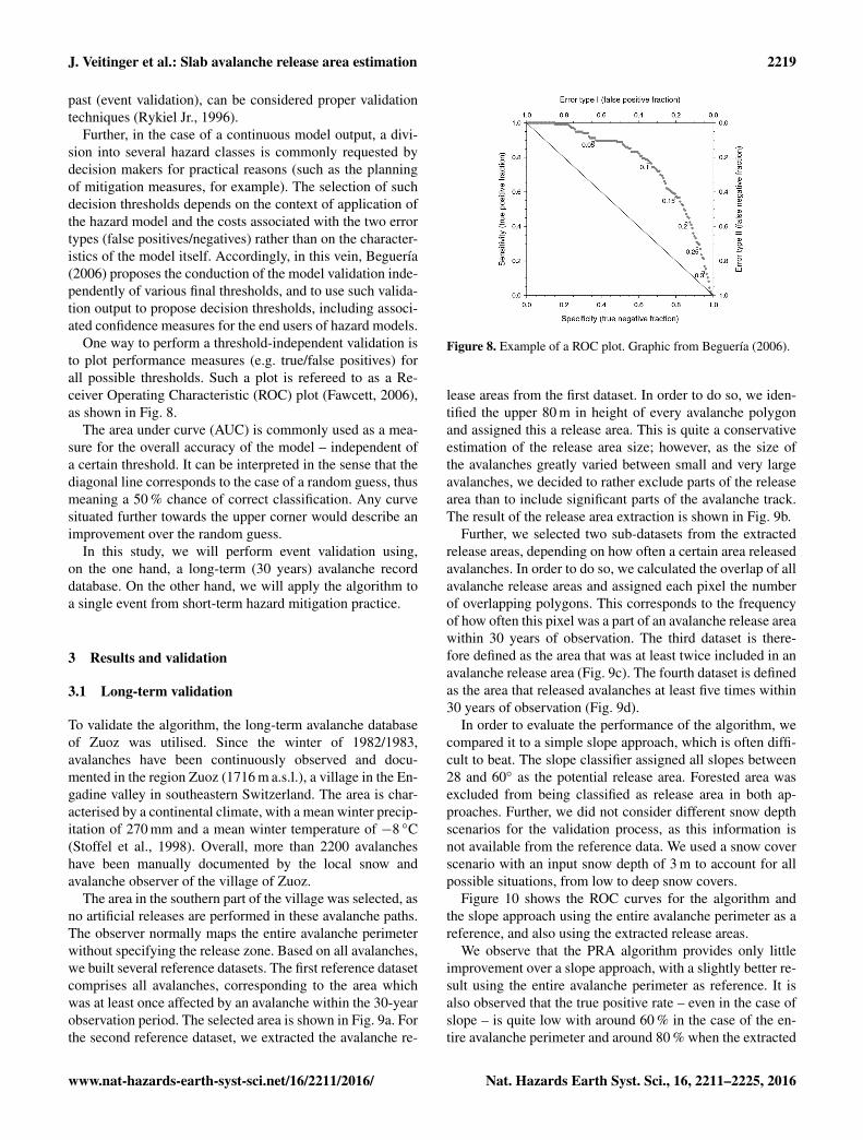
One way to perform a threshold-independent validation isto plot performance measures (e.g. true/false positives) forall possible thresholds. Such a plot is refereed to as a Re-ceiver Operating Characteristic (ROC) plot (Fawcett, 2006),as shown in Fig. 8.

The area under curve (AUC) is commonly used as a mea-sure for the overall accuracy of the model – independent ofa certain threshold. It can be interpreted in the sense that thediagonal line corresponds to the case of a random guess, thusmeaning a 50 % chance of correct classification. Any curvesituated further towards the upper corner would describe animprovement over the random guess.

In this study, we will perform event validation using,on the one hand, a long-term (30 years) avalanche recorddatabase. On the other hand, we will apply the algorithm toa single event from short-term hazard mitigation practice.

3 Results and validation

3.1 Long-term validation

To validate the algorithm, the long-term avalanche databaseof Zuoz was utilised. Since the winter of 1982/1983,avalanches have been continuously observed and docu-mented in the region Zuoz (1716 m a.s.l.), a village in the En-gadine valley in southeastern Switzerland. The area is char-acterised by a continental climate, with a mean winter precip-itation of 270 mm and a mean winter temperature of −8 ◦C(Stoffel et al., 1998). Overall, more than 2200 avalancheshave been manually documented by the local snow andavalanche observer of the village of Zuoz.

The area in the southern part of the village was selected, asno artificial releases are performed in these avalanche paths.The observer normally maps the entire avalanche perimeterwithout specifying the release zone. Based on all avalanches,we built several reference datasets. The first reference datasetcomprises all avalanches, corresponding to the area whichwas at least once affected by an avalanche within the 30-yearobservation period. The selected area is shown in Fig. 9a. Forthe second reference dataset, we extracted the avalanche re-

Figure 8. Example of a ROC plot. Graphic from Beguería (2006).

lease areas from the first dataset. In order to do so, we iden-tified the upper 80 m in height of every avalanche polygonand assigned this a release area. This is quite a conservativeestimation of the release area size; however, as the size ofthe avalanches greatly varied between small and very largeavalanches, we decided to rather exclude parts of the releasearea than to include significant parts of the avalanche track.The result of the release area extraction is shown in Fig. 9b.

Further, we selected two sub-datasets from the extractedrelease areas, depending on how often a certain area releasedavalanches. In order to do so, we calculated the overlap of allavalanche release areas and assigned each pixel the numberof overlapping polygons. This corresponds to the frequencyof how often this pixel was a part of an avalanche release areawithin 30 years of observation. The third dataset is there-fore defined as the area that was at least twice included in anavalanche release area (Fig. 9c). The fourth dataset is definedas the area that released avalanches at least five times within30 years of observation (Fig. 9d).

In order to evaluate the performance of the algorithm, wecompared it to a simple slope approach, which is often diffi-cult to beat. The slope classifier assigned all slopes between28 and 60◦ as the potential release area. Forested area wasexcluded from being classified as release area in both ap-proaches. Further, we did not consider different snow depthscenarios for the validation process, as this information isnot available from the reference data. We used a snow coverscenario with an input snow depth of 3 m to account for allpossible situations, from low to deep snow covers.

Figure 10 shows the ROC curves for the algorithm andthe slope approach using the entire avalanche perimeter as areference, and also using the extracted release areas.

We observe that the PRA algorithm provides only littleimprovement over a slope approach, with a slightly better re-sult using the entire avalanche perimeter as reference. It isalso observed that the true positive rate – even in the case ofslope – is quite low with around 60 % in the case of the en-tire avalanche perimeter and around 80 % when the extracted



Figure 9. Maps of observed avalanches within 30 years of observation south of Zuoz showing in red (a) the entire avalanche perimeter of allavalanches, (b) the extracted release areas of all avalanches, (c) the extracted avalanche release area that released avalanches at least twiceand (d) the extracted avalanche release area that released avalanches at least five times.

Figure 10. ROC curves for the PRA algorithm and slope for (a) the whole avalanche perimeter and (b) the extracted release areas.

release areas are taken as a reference. Whilst this can be ex-plained with the significant proportion of avalanche track andrun-out zone erroneously included in the reference datasetwhen using the full avalanche outline, this is not the case forthe extracted release areas. In actual fact, a true positive rateof 80 % for the slope classifier indicates that one-fifth of theavalanches were mapped in areas flatter than 28◦ or steeperthan 60◦. As avalanches are very unlikely in such regions,the deviations must be attributed to errors in the mappingprocess. As avalanches were mostly mapped from the roadin the valley bottom on a 1 : 25 000 m map, deviations up toseveral tens of metres in the location of the avalanches arelikely, explaining the erroneously mapped avalanches.

Figure 11 shows the classification result for the release ar-eas that occurred at least two and at least five times, respec-tively.

In this case, we observe that the PRA algorithm shows amore pronounced improvement compared to the slope classi-fier, suggesting that especially frequent avalanches are morereliably detected with the PRA algorithm. The fact that thetrue positive rate increases to around 90 % in the case of theavalanches that released avalanches at least five times showsthat the mapping error is reduced by taking the overlay ofseveral avalanches. Approximately 10 % of the avalanchesstill remain erroneously classified.



Figure 11. ROC curves for the PRA algorithm and slope for areas for which release occurred at least (a) twice and (b) five times.

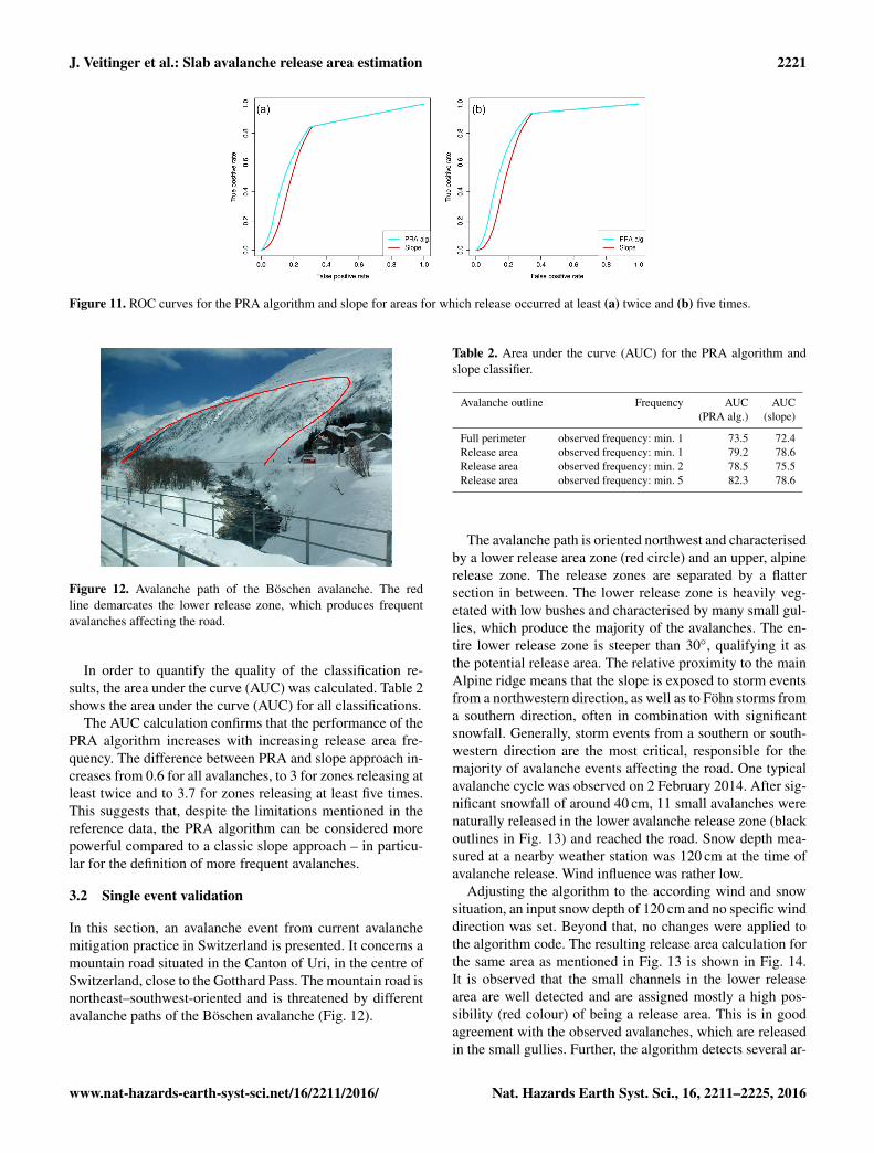
Figure 12. Avalanche path of the Böschen avalanche. The redline demarcates the lower release zone, which produces frequentavalanches affecting the road.

In order to quantify the quality of the classification re-sults, the area under the curve (AUC) was calculated. Table 2shows the area under the curve (AUC) for all classifications.

The AUC calculation confirms that the performance of thePRA algorithm increases with increasing release area fre-quency. The difference between PRA and slope approach in-creases from 0.6 for all avalanches, to 3 for zones releasing atleast twice and to 3.7 for zones releasing at least five times.This suggests that, despite the limitations mentioned in thereference data, the PRA algorithm can be considered morepowerful compared to a classic slope approach – in particu-lar for the definition of more frequent avalanches.

3.2 Single event validation

In this section, an avalanche event from current avalanchemitigation practice in Switzerland is presented. It concerns amountain road situated in the Canton of Uri, in the centre ofSwitzerland, close to the Gotthard Pass. The mountain road isnortheast–southwest-oriented and is threatened by differentavalanche paths of the Böschen avalanche (Fig. 12).

Table 2. Area under the curve (AUC) for the PRA algorithm andslope classifier.

Avalanche outline Frequency AUC AUC(PRA alg.) (slope)

Full perimeter observed frequency: min. 1 73.5 72.4Release area observed frequency: min. 1 79.2 78.6Release area observed frequency: min. 2 78.5 75.5Release area observed frequency: min. 5 82.3 78.6

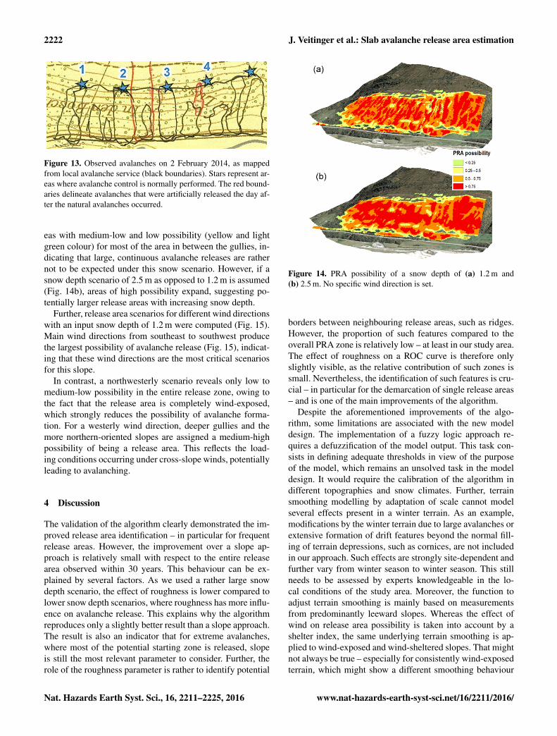
The avalanche path is oriented northwest and characterisedby a lower release area zone (red circle) and an upper, alpinerelease zone. The release zones are separated by a flattersection in between. The lower release zone is heavily veg-etated with low bushes and characterised by many small gul-lies, which produce the majority of the avalanches. The en-tire lower release zone is steeper than 30◦, qualifying it asthe potential release area. The relative proximity to the mainAlpine ridge means that the slope is exposed to storm eventsfrom a northwestern direction, as well as to Föhn storms froma southern direction, often in combination with significantsnowfall. Generally, storm events from a southern or south-western direction are the most critical, responsible for themajority of avalanche events affecting the road. One typicalavalanche cycle was observed on 2 February 2014. After sig-nificant snowfall of around 40 cm, 11 small avalanches werenaturally released in the lower avalanche release zone (blackoutlines in Fig. 13) and reached the road. Snow depth mea-sured at a nearby weather station was 120 cm at the time ofavalanche release. Wind influence was rather low.

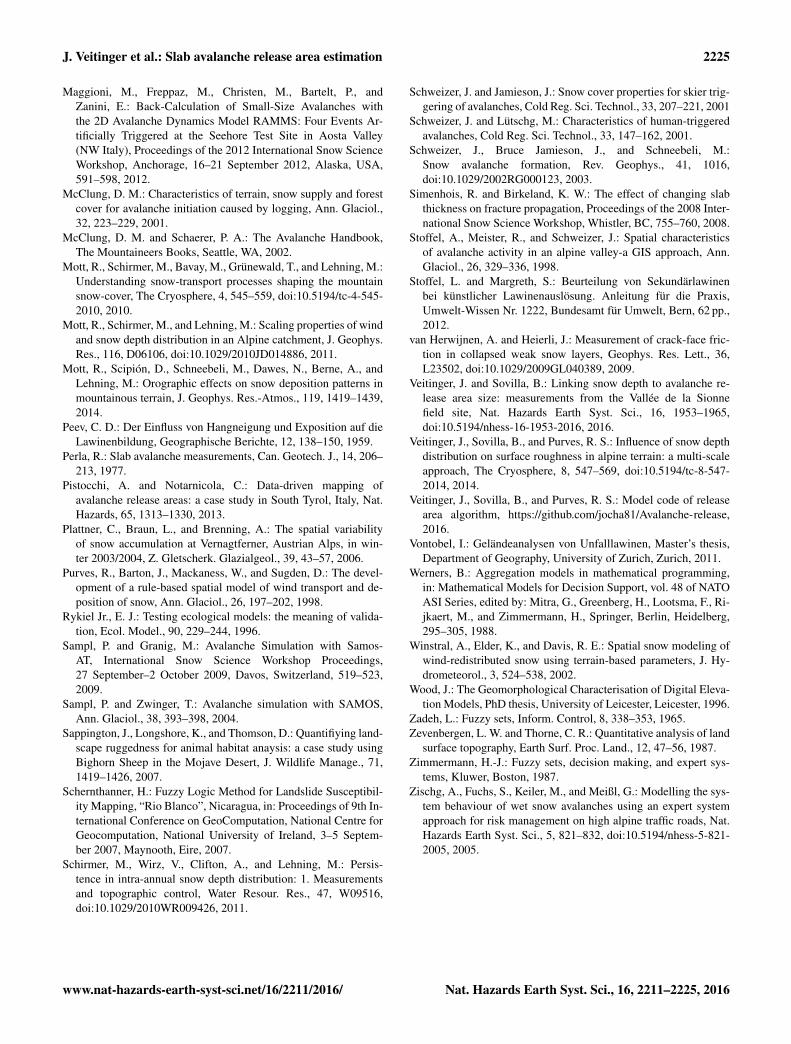
Adjusting the algorithm to the according wind and snowsituation, an input snow depth of 120 cm and no specific winddirection was set. Beyond that, no changes were applied tothe algorithm code. The resulting release area calculation forthe same area as mentioned in Fig. 13 is shown in Fig. 14.It is observed that the small channels in the lower releasearea are well detected and are assigned mostly a high pos-sibility (red colour) of being a release area. This is in goodagreement with the observed avalanches, which are releasedin the small gullies. Further, the algorithm detects several ar-



Figure 13. Observed avalanches on 2 February 2014, as mappedfrom local avalanche service (black boundaries). Stars represent ar-eas where avalanche control is normally performed. The red bound-aries delineate avalanches that were artificially released the day af-ter the natural avalanches occurred.

eas with medium-low and low possibility (yellow and lightgreen colour) for most of the area in between the gullies, in-dicating that large, continuous avalanche releases are rathernot to be expected under this snow scenario. However, if asnow depth scenario of 2.5 m as opposed to 1.2 m is assumed(Fig. 14b), areas of high possibility expand, suggesting po-tentially larger release areas with increasing snow depth.

Further, release area scenarios for different wind directionswith an input snow depth of 1.2 m were computed (Fig. 15).Main wind directions from southeast to southwest producethe largest possibility of avalanche release (Fig. 15), indicat-ing that these wind directions are the most critical scenariosfor this slope.

In contrast, a northwesterly scenario reveals only low tomedium-low possibility in the entire release zone, owing tothe fact that the release area is completely wind-exposed,which strongly reduces the possibility of avalanche forma-tion. For a westerly wind direction, deeper gullies and themore northern-oriented slopes are assigned a medium-highpossibility of being a release area. This reflects the load-ing conditions occurring under cross-slope winds, potentiallyleading to avalanching.

4 Discussion

The validation of the algorithm clearly demonstrated the im-proved release area identification – in particular for frequentrelease areas. However, the improvement over a slope ap-proach is relatively small with respect to the entire releasearea observed within 30 years. This behaviour can be ex-plained by several factors. As we used a rather large snowdepth scenario, the effect of roughness is lower compared tolower snow depth scenarios, where roughness has more influ-ence on avalanche release. This explains why the algorithmreproduces only a slightly better result than a slope approach.The result is also an indicator that for extreme avalanches,where most of the potential starting zone is released, slopeis still the most relevant parameter to consider. Further, therole of the roughness parameter is rather to identify potential

Figure 14. PRA possibility of a snow depth of (a) 1.2 m and(b) 2.5 m. No specific wind direction is set.

borders between neighbouring release areas, such as ridges.However, the proportion of such features compared to theoverall PRA zone is relatively low – at least in our study area.The effect of roughness on a ROC curve is therefore onlyslightly visible, as the relative contribution of such zones issmall. Nevertheless, the identification of such features is cru-cial – in particular for the demarcation of single release areas– and is one of the main improvements of the algorithm.

Despite the aforementioned improvements of the algo-rithm, some limitations are associated with the new modeldesign. The implementation of a fuzzy logic approach re-quires a defuzzification of the model output. This task con-sists in defining adequate thresholds in view of the purposeof the model, which remains an unsolved task in the modeldesign. It would require the calibration of the algorithm indifferent topographies and snow climates. Further, terrainsmoothing modelling by adaptation of scale cannot modelseveral effects present in a winter terrain. As an example,modifications by the winter terrain due to large avalanches orextensive formation of drift features beyond the normal fill-ing of terrain depressions, such as cornices, are not includedin our approach. Such effects are strongly site-dependent andfurther vary from winter season to winter season. This stillneeds to be assessed by experts knowledgeable in the lo-cal conditions of the study area. Moreover, the function toadjust terrain smoothing is mainly based on measurementsfrom predominantly leeward slopes. Whereas the effect ofwind on release area possibility is taken into account by ashelter index, the same underlying terrain smoothing is ap-plied to wind-exposed and wind-sheltered slopes. That mightnot always be true – especially for consistently wind-exposedterrain, which might show a different smoothing behaviour



Figure 15. PRA possibility of (a) a southerly wind direction, (b) a southwesterly wind direction, (c) a westerly wind direction and (d) anorthwesterly wind direction. Snow depth is set to 1.2 m.

to that found in our measurements. More studies in wind-exposed terrain would be necessary in an effort to understandterrain smoothing in such a type of terrain. Still, the practicalexample clearly demonstrates that terrain roughness, whenadjusted as a function of snow distribution, allows the as-sessment of the influence of terrain smoothing on potentialrelease area size and location.

It was further demonstrated that the integration of a windshelter parameter allows the definition of release area scenar-ios to be a function of a main wind direction. Yet it is evidentthat wind influence is strongly variable and often deviatesfrom the main wind direction (Mott and Lehning, 2011). Lo-cal winds strongly affect precipitation patterns near to theground (Mott et al., 2014). In addition, wind speeds andcoarse-scale sheltering effects through neighbouring moun-tain ridges also affect snow distribution. Such effects can-not be captured by a geomorphometric wind shelter index;this would require the physical modelling of the snow cover.Nevertheless, local experts aware of local wind effects andthe loading behaviours of avalanche-prone slopes may inte-grate this knowledge through adequate setting of the windshelter parameter.

5 Conclusions

We presented a new GIS tool for release area definition basedon a fuzzy logic classification approach. We implementeda roughness parameter in combination with a simple proce-dure to approximate winter terrain roughness from a summer

DTM. We showed that, for given snow cover scenarios, acharacteristic scale with maximum correlation between ter-rain roughness and snow surface roughness exists. This find-ing allows us to adapt the scale of the roughness parameter asa function of snow depth. In combination with a continuousclassification output, the algorithm improves the definition ofrelease areas, in particular for frequent avalanches.

Further, the algorithm can be applied in any mountainousareas where slab avalanches may occur. By modifying thefuzzy membership functions in Sect. 2.4, the algorithm couldbe easily adapted to other snow climates, such as coastal orHimalayan regions, where avalanches may occur in steeperareas than the Alps or the Rocky Mountains.

With regard to hazard mapping, the algorithm provides ad-ditional criteria for the partitioning of the whole potential re-lease in adequate sub-basins, by detecting fine-scale terrainfeatures, which serve as delimiting borders for less extremeavalanches. The algorithm further allows the assessment ofsnow influence on terrain morphology and, consequently, thepotential release area size and location for different snowcover scenarios. Both factors provide additional informationfor an avalanche expert in charge of designing design eventswith different return periods. This further enables avalancheexperts to objectivise and justify their decisions. However,the challenge of release area partitioning in very homoge-neous terrain remains, as the algorithm can only consider ter-rain changes as possible separation borders.

With respect to short-term hazard assessment, we couldshow that the new tool is able to potentially reproduceavalanche release areas, where microtopography plays a de-



cisive role. The preliminary results suggest that the influenceof the snow cover is realistically modelled. The integrationof a wind shelter index enables the user to define release areascenarios as a function of the main wind direction, enabling,for example, safety personnel, to assess release areas as afunction of single storm events. However, the algorithm isnot applicable as a forecasting tool, as snow stability is cur-rently not included in the parameters. In order to make thisapproach amenable, future research activity could thereforefocus on the coupling of the algorithm with snowpack condi-tions.

6 Data availability

The data used in this publication are property of the WSLInstitute for Snow and Avalanche Research SLF. The dataare available by submitting a specific request to Betty Sovilla([email protected]).

Acknowledgements. Funding for this research has been providedthrough the Interreg projects STRADA and STRADA 2.0 by thefollowing partners: Amt für Wald Graubünden, Canton du Valais –Service de forêts et paysage, Regione Lombardia, ARPA Lombar-dia, ARPA Piemonte and Regione Autonoma Valle d’Aosta. Theauthors thank Stefan Margreth for providing data for the practicalexample.

Edited by: S. TintiReviewed by: H. Schernthanner and one anonymous referee

References

Andres, A. J. and Cía, J. C.: Mapping of avalanche start zones sus-ceptibility: Arazas basin, Ordesa and Monte Perdido NationalPark (Spanish Pyrenees), J. Maps, 8, 14–21, 2012.

Barbolini, M., Gruber, U., Keylock, C. J., Naaim, M., and Savim, F.:Application of statistical and hydraulic-continuum dense-snowavalanche models to five real European sites, Cold Reg. Sci.Technol., 31, 133–149, 2000.

Barbolini, M., Pagliardi, M., Ferro, F., and Corradeghini, P.:Avalanche hazard mapping over large undocumented areas, Nat.Hazards, 56, 451–464, 2011.

Beguería, S.: Validation and evaluation of predictive models in haz-ard assessment and risk management, Nat. Hazards, 37, 315–329, 2006.

Blöschl, G.: Scaling issues in snow hydrology, Hydrol. Process., 13,2149–2175, 1999.

Brenning, A.: Statistical geocomputing combining R and SAGA:the example of landslide susceptibility analysis with general-ized additive models, in: SAGA – Seconds Out, vol. 19, editedby: Boehner, J., Blaschke, T., and Montanarella, L., HamburgerBeitraege zur Physischen Geographie und Landschaftsoekologie,Hamburg, Germany, 23–32, 2008.

Bühler, Y., Marty, M., and Ginzler, C.: High resolution DEM gener-ation in High-Alpine terrain using airborne remote sensing tech-niques, Trans. GIS, 16, 635–647, 2012.

Bühler, Y., Kumar, S., Veitinger, J., Christen, M., Stoffel, A., andSnehmani: Automated identification of potential snow avalancherelease areas based on digital elevation models, Nat. HazardsEarth Syst. Sci., 13, 1321–1335, doi:10.5194/nhess-13-1321-2013, 2013.

Caswell, H.: The validation problem, Syst. Anal. Simul. Ecol., 4,313–325, 1976.

Christen, M., Kowalski, J., and Bartelt, P.: RAMMS: numerical sim-ulation of dense snow avalanches in three-dimensional terrain,Cold Reg. Sci. Technol., 63, 1–14, 2010.

Cia, J. C., Andrés, A. J., and Magallón, A. M.: A proposal foravalanche susceptibility mapping in the Pyrenees using GIS: theFormigal-Peyreget area (Sheet 145-I; scale 1 : 25.000), J. Maps,10, 203–210, 2014.

Dreier, L., Bühler, Y., Steinkogler, W., Feistl, T., and Bartelt, P.:Modelling Small and Frequent Avalanches, Proceedings of the2014 International Snow Science Workshop, 29 September–3 October 2014, Banff, Alberta, Canada, 649–656, 2014.

Erickson, T. A., Williams, M. W., and Winstral, A.: Persistenceof topographic controls on the spatial distribution of snow inrugged mountain terrain, Colorado, US, Water Resour. Res., 41,W04014, doi:10.1029/2003WR002973, 2005.

Evans, I. S.: An integrated system of terrain analysis and slope map-ping, Z. Geomorphol. Supp., 36, 274–295, 1980.

Fawcett, T.: An introduction to ROC analysis, Pattern Recogn. Lett.,27, 861–874, 2006.

Gauer, P.: Numerical modeling of blowing and drifting snow inAlpine terrain, J. Glaciol., 47, 97–110, 2001.

Ghinoi, A. and Chung, C.-J.: STARTER: a statistical GIS-basedmodel for the prediction of snow avalanche susceptibility usingterrain features–application to Alta Val Badia, Italian Dolomites,Geomorphology, 66, 305–325, 2005.

Goodchild, M. F. and Quattrochi, D. A.: Scale, Multiscaling, Re-mote Sensing, and GIS, in: Scale in remote sensing and GIS,edited by: Goodchild, M. F. and Quattrochi, D. A., CRC Press,Boca Raton, FL, 1–11, 1997.

Grohmann, C., Smith, M., and Riccomini, C.: Multiscale analysis oftopographic surface roughness in the Midland Valley, Scotland,IEEE T. Geosci. Remote, 49, 1200–1213, 2011.

Gruber, U. and Sardemann, S.: High-frequency avalanches: releasearea characteristics and run-out distances, Cold Reg. Sci. Tech-nol., 37, 439–451, 2003.

Hobson, R. D.: Surface roughness in topography: a quantitative ap-proach, Harper and Row, Methuer, London, 221–245, 1972.

Jang, J.-S. R. and Sun, C.-T.: Neuro-fuzzy and soft computing: acomputational approach to learning and machine intelligence,Prentice-Hall, Inc., Upper Saddle River, NJ, USA, 1997.

Lehning, M., Löwe, H., Ryser, M., and Raderschall, N.:Inhomogeneous precipitation distribution and snow trans-port in steep terrain, Water Resour. Res., 44, W07404,doi:10.1029/2007WR006545, 2008.

Lehning, M., Grünewald, T., and Schirmer, M.: Mountainsnow distribution governed by an altitudinal gradientand terrain roughness, Geophys. Res. Lett., 38, L19504,doi:10.1029/2011GL048927, 2011.

Maggioni, M. and Gruber, U.: The influence of topographic param-eters on avalanche release dimension and frequency, Cold Reg.Sci. Technol., 37, 407–419, 2003.


http://dx.doi.org/10.5194/nhess-13-1321-2013


http://dx.doi.org/10.1029/2003WR002973

http://dx.doi.org/10.1029/2007WR006545

http://dx.doi.org/10.1029/2011GL048927


Maggioni, M., Freppaz, M., Christen, M., Bartelt, P., andZanini, E.: Back-Calculation of Small-Size Avalanches withthe 2D Avalanche Dynamics Model RAMMS: Four Events Ar-tificially Triggered at the Seehore Test Site in Aosta Valley(NW Italy), Proceedings of the 2012 International Snow ScienceWorkshop, Anchorage, 16–21 September 2012, Alaska, USA,591–598, 2012.

McClung, D. M.: Characteristics of terrain, snow supply and forestcover for avalanche initiation caused by logging, Ann. Glaciol.,32, 223–229, 2001.

McClung, D. M. and Schaerer, P. A.: The Avalanche Handbook,The Mountaineers Books, Seattle, WA, 2002.

Mott, R., Schirmer, M., Bavay, M., Grünewald, T., and Lehning, M.:Understanding snow-transport processes shaping the mountainsnow-cover, The Cryosphere, 4, 545–559, doi:10.5194/tc-4-545-2010, 2010.

Mott, R., Schirmer, M., and Lehning, M.: Scaling properties of windand snow depth distribution in an Alpine catchment, J. Geophys.Res., 116, D06106, doi:10.1029/2010JD014886, 2011.

Mott, R., Scipión, D., Schneebeli, M., Dawes, N., Berne, A., andLehning, M.: Orographic effects on snow deposition patterns inmountainous terrain, J. Geophys. Res.-Atmos., 119, 1419–1439,2014.

Peev, C. D.: Der Einfluss von Hangneigung und Exposition auf dieLawinenbildung, Geographische Berichte, 12, 138–150, 1959.

Perla, R.: Slab avalanche measurements, Can. Geotech. J., 14, 206–213, 1977.

Pistocchi, A. and Notarnicola, C.: Data-driven mapping ofavalanche release areas: a case study in South Tyrol, Italy, Nat.Hazards, 65, 1313–1330, 2013.

Plattner, C., Braun, L., and Brenning, A.: The spatial variabilityof snow accumulation at Vernagtferner, Austrian Alps, in win-ter 2003/2004, Z. Gletscherk. Glazialgeol., 39, 43–57, 2006.

Purves, R., Barton, J., Mackaness, W., and Sugden, D.: The devel-opment of a rule-based spatial model of wind transport and de-position of snow, Ann. Glaciol., 26, 197–202, 1998.

Rykiel Jr., E. J.: Testing ecological models: the meaning of valida-tion, Ecol. Model., 90, 229–244, 1996.

Sampl, P. and Granig, M.: Avalanche Simulation with Samos-AT, International Snow Science Workshop Proceedings,27 September–2 October 2009, Davos, Switzerland, 519–523,2009.

Sampl, P. and Zwinger, T.: Avalanche simulation with SAMOS,Ann. Glaciol., 38, 393–398, 2004.

Sappington, J., Longshore, K., and Thomson, D.: Quantifiying land-scape ruggedness for animal habitat anaysis: a case study usingBighorn Sheep in the Mojave Desert, J. Wildlife Manage., 71,1419–1426, 2007.

Schernthanner, H.: Fuzzy Logic Method for Landslide Susceptibil-ity Mapping, “Rio Blanco”, Nicaragua, in: Proceedings of 9th In-ternational Conference on GeoComputation, National Centre forGeocomputation, National University of Ireland, 3–5 Septem-ber 2007, Maynooth, Eire, 2007.

Schirmer, M., Wirz, V., Clifton, A., and Lehning, M.: Persis-tence in intra-annual snow depth distribution: 1. Measurementsand topographic control, Water Resour. Res., 47, W09516,doi:10.1029/2010WR009426, 2011.

Schweizer, J. and Jamieson, J.: Snow cover properties for skier trig-gering of avalanches, Cold Reg. Sci. Technol., 33, 207–221, 2001

Schweizer, J. and Lütschg, M.: Characteristics of human-triggeredavalanches, Cold Reg. Sci. Technol., 33, 147–162, 2001.

Schweizer, J., Bruce Jamieson, J., and Schneebeli, M.:Snow avalanche formation, Rev. Geophys., 41, 1016,doi:10.1029/2002RG000123, 2003.

Simenhois, R. and Birkeland, K. W.: The effect of changing slabthickness on fracture propagation, Proceedings of the 2008 Inter-national Snow Science Workshop, Whistler, BC, 755–760, 2008.

Stoffel, A., Meister, R., and Schweizer, J.: Spatial characteristicsof avalanche activity in an alpine valley-a GIS approach, Ann.Glaciol., 26, 329–336, 1998.

Stoffel, L. and Margreth, S.: Beurteilung von Sekundärlawinenbei künstlicher Lawinenauslösung. Anleitung für die Praxis,Umwelt-Wissen Nr. 1222, Bundesamt für Umwelt, Bern, 62 pp.,2012.

van Herwijnen, A. and Heierli, J.: Measurement of crack-face fric-tion in collapsed weak snow layers, Geophys. Res. Lett., 36,L23502, doi:10.1029/2009GL040389, 2009.

Veitinger, J. and Sovilla, B.: Linking snow depth to avalanche re-lease area size: measurements from the Vallée de la Sionnefield site, Nat. Hazards Earth Syst. Sci., 16, 1953–1965,doi:10.5194/nhess-16-1953-2016, 2016.

Veitinger, J., Sovilla, B., and Purves, R. S.: Influence of snow depthdistribution on surface roughness in alpine terrain: a multi-scaleapproach, The Cryosphere, 8, 547–569, doi:10.5194/tc-8-547-2014, 2014.

Veitinger, J., Sovilla, B., and Purves, R. S.: Model code of releasearea algorithm, https://github.com/jocha81/Avalanche-release,2016.

Vontobel, I.: Geländeanalysen von Unfalllawinen, Master’s thesis,Department of Geography, University of Zurich, Zurich, 2011.

Werners, B.: Aggregation models in mathematical programming,in: Mathematical Models for Decision Support, vol. 48 of NATOASI Series, edited by: Mitra, G., Greenberg, H., Lootsma, F., Ri-jkaert, M., and Zimmermann, H., Springer, Berlin, Heidelberg,295–305, 1988.

Winstral, A., Elder, K., and Davis, R. E.: Spatial snow modeling ofwind-redistributed snow using terrain-based parameters, J. Hy-drometeorol., 3, 524–538, 2002.

Wood, J.: The Geomorphological Characterisation of Digital Eleva-tion Models, PhD thesis, University of Leicester, Leicester, 1996.

Zadeh, L.: Fuzzy sets, Inform. Control, 8, 338–353, 1965.Zevenbergen, L. W. and Thorne, C. R.: Quantitative analysis of land

surface topography, Earth Surf. Proc. Land., 12, 47–56, 1987.Zimmermann, H.-J.: Fuzzy sets, decision making, and expert sys-

tems, Kluwer, Boston, 1987.Zischg, A., Fuchs, S., Keiler, M., and Meißl, G.: Modelling the sys-

tem behaviour of wet snow avalanches using an expert systemapproach for risk management on high alpine traffic roads, Nat.Hazards Earth Syst. Sci., 5, 821–832, doi:10.5194/nhess-5-821-2005, 2005.


http://dx.doi.org/10.5194/tc-4-545-2010

http://dx.doi.org/10.5194/tc-4-545-2010

http://dx.doi.org/10.1029/2010JD014886

http://dx.doi.org/10.1029/2010WR009426

http://dx.doi.org/10.1029/2002RG000123

http://dx.doi.org/10.1029/2009GL040389


http://dx.doi.org/10.5194/tc-8-547-2014

http://dx.doi.org/10.5194/tc-8-547-2014

https://github.com/jocha81/Avalanche-release



Documents

Potential slab avalanche release area identiﬁcation from ... · Received: 8 September 2015 ... which cause the vast majority of ... the fuzzy logic approach in an effort to deal