Embed Size (px)
Citation preview

remote sensing
Article
Potential of ENVISAT Radar Altimetry for WaterLevel Monitoring in the Pantanal Wetland
Denise Dettmering *, Christian Schwatke, Eva Boergens and Florian Seitz
Deutsches Geodätisches Forschungsinstitut der Technischen Universität München (DGFI-TUM),Arcisstrasse 21, 80333 München, Germany; [email protected] (C.S.); [email protected] (E.B.);[email protected] (F.S.)* Correspondence: [email protected]; Tel.: +49-89-23031-1198
Academic Editors: Javier Bustamante, Magaly Koch and Prasad S. ThenkabailReceived: 4 May 2016; Accepted: 11 July 2016; Published: 14 July 2016
Abstract: Wetlands are important ecosystems playing an essential role for continental waterregulation and the hydrologic cycle. Moreover, they are sensitive to climate changes as well asanthropogenic influences, such as land-use or dams. However, the monitoring of these regionsis challenging as they are normally located in remote areas without in situ measurement stations.Radar altimetry provides important measurements for monitoring and analyzing water levelvariations in wetlands and flooded areas. Using the example of the Pantanal region in SouthAmerica, this study demonstrates the capability and limitations of ENVISAT radar altimeter formonitoring water levels in inundation areas. By applying an innovative processing methodconsisting of a rigorous data screening by means of radar echo classification as well as an optimizedwaveform retracking, water level time series with respect to a global reference and with a temporalresolution of about one month are derived. A comparison between altimetry-derived heightvariations and six in situ time series reveals accuracies of 30 to 50 cm RMS. The derived waterlevel time series document seasonal height variations of up to 1.5 m amplitude with maximumwater levels between January and June. Large scale geographical pattern of water heights arevisible within the wetland. However, some regions of the Pantanal show water level variations lessthan a few decimeter, which is below the accuracies of the method. These areas cannot be reliablymonitored by ENVISAT.
Keywords: satellite altimetry; wetlands; Pantanal; water level; ENVISAT; inundation
1. Introduction
Radar altimetry was designed to provide highly accurate measurements of sea surface heightsover open ocean areas on a global scale. One important application of altimetry is still in thearea of oceanography where the datasets help to improve our knowledge of ocean circulation,mesoscale variability, ocean tides, sea level change, etc. [1–3]. However, since the launch of theTOPEX/Poseidon satellite in 1992 alternative application areas are grown and nowadays, satellitealtimetry is also used for the determination of ice sheet elevations and inland water level monitoring(e.g., [4,5]).
In contrast to open ocean altimeter measurements, reflected radar echoes (so-called waveforms)from other surface types show different shapes depending on the reflectors within the altimeterfootprint. A careful data editing and reprocessing is required in order to derive reliable and highlyaccurate range measurements from the received waveforms—a process called retracking. Within thelast decade, various investigations on new retracking algorithms have been made in order to enhancethe accuracy of coastal and inland water level estimation. In particular, progress has been maderegarding lakes and reservoirs (e.g., [6,7]) and large rivers (e.g., [8–10]). Actually, at least four global
Remote Sens. 2016, 8, 596; doi:10.3390/rs8070596 www.mdpi.com/journal/remotesensing

Remote Sens. 2016, 8, 596 2 of 21
databases exist providing inland water level time series for a variety of water bodies based on severalaltimeter missions [11–14]. Their results are highly valuable for applications in continental hydrology,especially given that other data sources such as in situ gauge stations are rapidly declining since about1980 [15].
In addition to water levels, information on the reflectivity of the surface can be derived fromsatellite altimetry. Over open ocean, the sea state, e.g., wind and waves, can be observed [16]and over land surfaces, the backscatter coefficient allows for the classification of different reflectors.For example, Papa et al. [17] used TOPEX/Poseidon dual-frequency backscatter values to investigatedifferent land surface types on a global scale. More recently, Le et al. [18] extended this study bymerging data from different missions (Jason-1, ENVISAT, and Jason-2). For both studies, the spatialresolution is sparse since only global or regional scales are examined.
Using radar altimetry for wetland water monitoring is both: (1) a great possibility for derivinghydrologic information in mostly remote areas where in large parts infrastructure is missing and noin situ observations are available and (2) a challenge for data processing as only small areas withopen water exist that change rapidly with time. Investigations using radar altimetry to study waterlevel variations of inundation areas and wetlands are rare. Smith and Berry [19] presented selectedwater level time series for various wetlands, among them the Pantanal. Their results are promisingbut a comprehensive validation of the results is missing. Moreover, some dedicated studies exist forthe Louisiana wetlands (e.g., Lee et al. [20] and Khajeh et al. [21]) and Poyang Lake watershed [22].Most of these studies do not provide satisfying results or lack comprehensive validations. Inaddition, some studies focused on rivers or river basins including inundation areas (floodplains)(e.g., Birkett et al. [23] and Frappart et al. [24], both using TOPEX/Poseidon data in the Amazonbasin.). The backscatter of radar altimeters was already used to study the variability of wetland extentas shown for example by Zakharova et al. [25] and Papa et al. [26]. However, due to the measurementgeometry along separate profiles a complete coverage of the area is not possible. Other remote sensingtechniques such as optical or radar images are more straight forward. Nevertheless, the altimeterbackscatter information is a valuable input for classifying inundation areas beneath the satellite trackand may help in fine-tuning the processing parameters to derive water levels from altimetry.
Focusing on the example of Pantanal, the present study investigates the capability of radaraltimetry to monitor water level variations of large inundation areas. The backscatter information isused to classify different inundation areas and to define water returns in order to perform a rigorousdata editing. The Pantanal is one of the largest wetlands worldwide. It is located in South America,mostly in Brazil with smaller parts in Bolivia and Paraguay. Several interesting studies exist on thisinundation area, mainly dealing with the extent of water areas and consequences for the ecosystem,among them Hamilton et al. [27], Hamilton et al. [28], Evans et al. [29], Evans and Costa [30],Girard et al. [31], and Padovani [32]. All these studies rely on sparse in situ gauging stations toderive water level time series. As far as the authors know, no dedicated and comprehensive study onusing radar altimetry for estimating water levels within the Pantanal exists.
This study proposes an innovative processing method based on automated altimeter dataselection by waveform classification and a dedicated waveform retracking. The results are carefullyvalidated and analyzed region-wide in order to detect spatial patterns of water level changes. Thepaper provides the first comprehensive study on the use of radar altimetry for estimating waterlevel variations within the Pantanal. However, the focus of the study is not on applications andmanagement of the Pantanal region but on the methodology and assessment of ENVISAT quality ininundated regions.
The paper is structured into four main parts: First, the study area and the used datasets areintroduced (Section 2). Afterwards, the data in the study area are analyzed concerning their capabilityto detect inundation areas (Section 3.1) as well as with respect to the spatial coverage (Section 3.2).Section 3 also presents the strategy for defining observation points (virtual stations). Section 4

Remote Sens. 2016, 8, 596 3 of 21
describes the method used for the computation of water level time series. The results are analyzedand discussed in Section 5.
2. Study Area and Used Datasets
2.1. The Pantanal
The Pantanal is one of the world’s largest wetlands. It is located in the center of South Americaand comprises an area of about 400 km × 250 km [33]. Since 2000, the Pantanal is a UNESCOBiosphere Reserve as well as partially a World Heritage Site. The whole region is characterized byseasonal inundation and desiccation with episodes of standing water and episodes of dry surfaceand subsurface water level below the rooting zone. The Pantanal is a complex of floodplains fromdifferent rivers and the inundation patterns vary depending on the source of floodwater [28]. For allsub-regions a fractional inundation area of at least 50% is reached for several months in most yearsbetween 1979 and 1987 [27]. The Pantanal is drained by the Paraguay River flowing in North-Southdirection. Its major tributaries are five larger rivers flowing mainly from east to west. Water levelseasonal fluctuations within the region are maximal for the Paraguay River with 2–5 m [33].
The region of the Pantanal floodplains is relatively flat with elevations between 80 to 150 m andterrain slopes of only 25 cm/km [33] with some isolated mountains (up to about 800 m) interspersed.The Pantanal is located within tropical climate and exhibits a marked wet season between Novemberand March and an annual rainfall of 1000–1500 mm across the whole basin [33]. The most commonvegetation in the Pantanal are savanna and mixtures of grassland with semi-deciduous forest. Treesusually have sparse canopies [27].
The present study comprises the whole Pantanal as well as the surrounding region within anarea between 22◦ and 15.5◦ southern latitude and between 60◦ and 54.5◦ western longitude. Thestudy area is illustrated in Figure 1.
−60˚
−60˚
−59˚
−59˚
−58˚
−58˚
−57˚
−57˚
−56˚
−56˚
−55˚
−55˚
−22˚
−21˚
−20˚
−19˚
−18˚
−17˚
−16˚
0 100
km
N
220
607P1
P2
Caceres
Cuiaba
Corumba
Porto Jofre
Sao Vicente
Coxim
Puerto Quijarro
Miranda
Campo Grande
Rondonopolis
Bahia Negra
Porto Murtinho
Caceres
Porto Cercado
Sao Jeronimo
Posada Taiama
Sao Francisco
Ladario
1 2
3 4 5
6 7 8
0
50
100
150
200
250
300
350
400
450
500
550
600
650
700
750
800
m
Figure 1. The Pantanal region with main settlements (black squares) and major rivers (blue).Background colors indicate topography taken from ETOPO01 [37]. ENVISAT satellite tracks areshown with gray lines and in situ gauging stations are illustrated by red triangles. Track parts of pass220 and 607 are highlighted by bold lines. The locations of the stations used in Section 4.3 (P1 and P2)are marked by black crosses. Crossover locations used for validation are numbered and indicated bygray circles.

Remote Sens. 2016, 8, 596 4 of 21
2.2. Altimeter Datasets
The study uses ENVISAT RA-2 [34] observations for estimating water levels in the Pantanal.This satellite altimetry mission provides profiled measurements along the satellites tracks with analong-track spatial resolution, which could reach to about 350 m (18 Hz measurements). Thecross-track resolution is lower (about 80 km) and depends on the satellite’s orbit. In principle,the missions ERS-2 and SARAL (using the same orbit as ENVISAT) are usable to extend the timeseries. Moreover, data from TOPEX/Poseidon and its successors Jason-1 and Jason-2 might be usedto improve the spatial and temporal resolution. However, this study focuses on ENVISAT since thedata quality of ERS is still not good enough, SARAL is not directly connected to ENVISAT (data gap2011/2012), and there are only two tracks of TOPEX/Jason over the Pantanal. The ENVISAT satellitetracks are illustrated in Figure 1.
All investigations are based on high-frequent altimeter waveforms extracted from SensorGeophysical Data Records (SGDR) version 2.1 files provided by ESA. The dataset covers a timeperiod of about eight years (2003–2010). For analyzing the spatial distribution of open water, Ku-bandaltimeter backscatter values from ice-1 retracking [34] are additionally used.
In order to correct the altimeter ranges for geophysical effects, external models are applied. Thisholds especially for the atmospheric corrections (troposphere delay as well as ionosphere delay)since radiometer and dual-frequency corrections are not reliable over inland areas. No sea statebias (SSB) corrections and no dynamic atmospheric corrections (DAC) are applied. Even thoughno multi-mission approach is followed, inter-mission biases are taken into account by applying radialerror corrections to all measurements. These corrections are computed by a global multi-missioncrossover analysis as described in Bosch et al. [35]. Their application ensures the estimation ofabsolute water levels, since the known offset (about 0.5 m) of ENVISAT heights is taken intoaccount. The ellipsoidal heights were converted to physical heights (i.e., normal heights) using the“EIGEN6c3stat“ geoid [36]. All geophysical corrections used within this study are summarized inTable 1.
Table 1. Geophysical corrections used in the study.
Correction Source/Model Reference
Wet troposphere ECMWF (2.5◦ × 2.0◦) for Vienna Mapping Functions (VMF1) Boehm et al. [38]Dry troposphere ECMWF (2.5◦ × 2.0◦) for Vienna Mapping Functions (VMF1) Boehm et al. [38]Ionosphere NOAA Ionosphere Climatology 2009 (NIC09) Scharroo and Smith [39]Solid Earth tides IERS Conventions 2003 McCarthy and Petit [40]Pole tides IERS Conventions 2003 McCarthy and Petit [40]Range bias MMXO14 Bosch et al. [35]
3. Inundation Patterns and Definition of Virtual Stations
Due to the satellite’s orbits a complete coverage of the whole area is not possible. Only a fewdedicated profiles can be measured. However, the spatial resolution along these profiles is extremelyhigh. A challenging task is the localization of open water areas and the definition of virtual stations.Since the inundation area changes significantly with time and most regions are not continuouslycovered by water it is difficult to define distinct measurement points. Moreover, the intention of thisstudy is to catch as much information as possible and to derive water levels also for occasionallyflooded locations.
Usually the definition of virtual stations is done manually or by using a map, e.g., Google Earthimagery [8]. This is difficult or even impossible in wetland areas due to small-scale temporal waterfluctuations. However, the altimeter instrument itself already provides some information on thereflectors within its footprint. The altimeter waveforms may be classified to separate different surfaceproperties (e.g., Desai et al. [41]). As an alternative, derived quantities such as the radar backscattercan be used.

Remote Sens. 2016, 8, 596 5 of 21
3.1. Inundation Pattern Along the Satellite Ground Tracks
The radar echoes as measured by the altimeter can be used to extract information on theproperties of the reflecting Earth surface. This can be done directly based on the waveforms or byinterpretation of derived quantities such as the backscatter coefficient σ0. The latter method is theeasiest way since one can use the given data sets and an own reprocessing is not required. Figure 2shows the Ku-band backscatter from ice-1 retracker for a short part (about 100 km) of one ENVISATtrack (pass 607; location highlighted in Figure 1). By defining a threshold (in this case 32 dB is used)one can classify measurements with large backscatters as water return with specular reflections [23].However, as can be seen from the negative values in the figure, the absolute level of the given valuesis not correct. Moreover, a direct comparison with other missions is not always possible. That is thereason for using waveform properties for the classification. In this paper, a combination of variouswaveform parameters (such as peakiness and maximum power) is used to define water returns (moredetails in Section 4.1). The results are very similar to the backscatter-based classification.
year
2004 2006 2008 2010
latitu
de [deg]
-17.2
-17.1
-17
-16.9
-16.8
-16.7
-16.6
-16.5
-16.4
-16.3
backscatter [dB]
-20
-10
0
10
20
30
40
50
60
longitude [deg]
-56.6 -56.5 -56.4 -56.3-17.2
-17.1
-17
-16.9
-16.8
-16.7
-16.6
-16.5
-16.4
-16.3
water returns [%]
0 50 100-17.2
-17.1
-17
-16.9
-16.8
-16.7
-16.6
-16.5
-16.4
-16.3
ETOPO01 height [m]
120 130-17.2
-17.1
-17
-16.9
-16.8
-16.7
-16.6
-16.5
-16.4
-16.3
Figure 2. Identification of water returns for part of ENVISAT pass 607. The left plot shows Ku-bandice-1 backscatter in [dB] for each measurement of each overflight. The second plot depicts thepercentage of water returns (hydroperiod) per 0.05 degree track segment as defined by waveformclassification. On the middle right the location of the measurements (red track) can be seen. Riversare taken from HydroSHEDS [42]. The last plot shows the terrain heights (from ETOPO01) along theENVISAT track.
In Figure 2 one can define some points along the track with permanent open water (rivers),since they show high backscatters over the whole time span. For other areas periodic changes ofbackscatter can be seen indicating regions with seasonal flooding. The location of rivers classified bythe altimetry backscatter is in good agreement with the rivers provided by HydroSHEDS [42]. Onlyone river (at latitude −16.88 degree) cannot be seen by the altimeter. It is not located in a valley andprobably very small. It is also not part of the CIA World data bank (WDB II) as used e.g., by GenericMapping Tools (GMT) [43]. However, this example illustrates that ENVISAT is able to detect riversand small open water areas without additional external information.
Thus, radar altimetry can be used to map the temporal variability of water areas in wetlands andto provide information on flood frequency and flood duration. In hydrology, different (non-tidal)wetland types are defined based on their hydroperiods, i.e., the percentage of time that water isstanding. In U.S. EPA [44], seven types are listed based on the general relationship between wetlandwater levels and hydric states. It is difficult to group the altimetry results into the seven originalclasses as long as the flood duration is not analyzed in detail. In this study, a classification into fourgroups is performed based on the percentage of water returns per track segment over the whole time

Remote Sens. 2016, 8, 596 6 of 21
span. This defines the inundation frequency for the different areas. If altimetry detects water inless than 20% of the time, the segment is classified as “mostly dry”. In cases where water is in thesegment for up to 50% of the time, the segment is “temporarily flooded”. This class also incorporates“intermittently flooded” areas. An area is defined as “seasonally flooded” when water is detected for50% to 90% of the time. At last, a segment is “permanently flooded” in case water is present in morethan 90% of the time. The definition of the four classes used is summarized in Table 2. Naturally, theclass limits are somehow arbitrary, since a distinct separation is hardly possible.
Table 2. Inundation classes derived from altimetry waveform classification.
Class Description Hydroperiod
1 mostly dry <20%2 temporarily flooded 20%–50%3 seasonally flooded 50%–90%4 open water or permanently flooded >90%
The corresponding classification results are shown in Figure 3. The left part of the figure showsthe percentage of water returns in small track segments and the middle part displays the derivedinundation classes. One can clearly identify the extent of the wetland even if no external informationon the boundaries are used to generate these plots. In addition, areas with open water throughout thewhole years can be identified: one around the Rio Paraguay South of Caceres and another at the lowerRio Taquari around 100 km North-East of Corumba. On the right-hand side of Figure 3 an externalclassification from GIEMS-D15 [45,46] is provided showing three states of inundation extent. As theseresults are mostly based on satellite images, they cover the whole Pantanal area. The spatial resolutionof about 450 m is the same for both data sets, however, the time periods differ significantly: whileGIEMS-D15 is based on data between 1993 and 2004 the altimetry data are from 2002–2011. Moreover,the inundation frequency is not necessarily directly connected to the inundation extent. This mightexplain some of the differences visible mainly in the central part of the Pantanal. ENVISAT classifieslarge parts west of Sao Vicente and north of Rio Taquari as open water whereas in GIEMS-D15 mainlythe Rio Taquari itself is visible. Since this region is characterized by many small rivers and small areasof standing open water it is not clear why it is not visible in GIEMS-D15. Similar discrepancies canalso be seen comparing GIEMS-D15 with MODIS-based results from Padovani [32] as presented inFluet-Chouinard et al. [45] (Figure 7, page 358). Moraes et al. [47] also reported open water betweenSao Francisco and Sao Vicente.
Figure 3. Percentage of water returns per 0.1 degree track segment (left) and derived inundationclasses (middle); both from waveform classification. The third plot (right) shows the GIEMS-D15inundation classes for comparison.

Remote Sens. 2016, 8, 596 7 of 21
3.2. Definition of Virtual Stations: Track Segmentation Concept
Radar altimetry can only provide water levels when the satellite’s footprint covers open water.In order to derive water level times series of inland waters so-called virtual stations (e.g., [48]) aredefined at locations where the satellite track crosses a lake or a river. Classically, this is done usinggiven time-independent water body maps or remote sensing images. Since the inundation patternwithin wetlands changes rapidly from one location to the next, it is challenging to define virtualstations offside larger rivers and lakes. However, these are the most interesting regions since no insitu datasets exist.
Instead of selecting single virtual stations all satellite tracks are separated in regular piecesof 0.05 degree (corresponding to about 6 km) and each of these track segments define one virtualstation. This ensures around 17 measurements per segment and overflight. The segmentation size is acompromise between a good data coverage and a high along-track spatial resolution. Small segmentsensure homogeneous conditions within the single compartments, e.g., similar hydrological conditionsand no terrain slope. Since clearly not all virtual stations will contain open water a careful datapre-processing is necessary in order to get rid of land-contaminated observations (see Section 4.1).
Due to the sparse cross-track spatial resolution of satellite altimetry some regions will be missedeven when using more than one repeat-track mission. This is related to the nadir measurementprinciple and the orbits of satellite altimetry and cannot be avoided.
The location of crossover points (where ascending and descending passes are crossing eachother) can be used to perform a validation (see Section 4.4.1).
4. Computation of Water Level Time Series
For each 0.05◦ track segment one time series of water level is computed. For this purpose, acareful data pre-processing is required since the data quality over inland water targets is not asgood as over open ocean. Especially waveforms contaminated by land should be excluded fromcomputations. Moreover, a dedicated retracking is recommended in order to increase the data quality.
For many applications the derivation of accuracies along with water levels is valuable. Thus, anerror information for each water height is derived in addition to the water level itself.
4.1. Waveform Classification
Since the definition of virtual stations is done automatically and not only in permanently floodedareas, not all altimeter measurements are usable. Due to the diversity of reflecting surfaces (e.g., openwater, swimming vegetation, flooded areas covered by vegetation, land,...) the altimeter waveformsshow a rich variety and different qualities. The elimination of unusable data from the processing isrealized by waveform classification.
This is done by applying selected thresholds on waveform-related statistical parameters suchas skewness, kurtosis, peakiness, maximum power, and signal-to-noise ratio. The method dividesthe altimeter returns into four major classes, one of them called “single peak” containing purequasi-specular waveforms as returned from small inland open water reflectors. This is the only classused in this study. Thus, the identification of the other classes is not discussed here. The identificationof the quasi-specular waveforms is based on the normalized peakiness that is computed from thewaveform power wi for i = 1...n and n = number o f bins by dividing the maximum power of thewaveform by the sum of the waveform power following Equation (1).
peakiness =max(wi)
∑ni=1 wi
(1)
A threshold of 0.5 is defined to identify inland water reflectors. Figure 4 shows two waveformexamples registered over inland. On the left-hand side a specular waveform with a peakiness of 0.53is plotted. The right-hand side displays a corrupted waveform (peakiness of 0.04). In this study,

Remote Sens. 2016, 8, 596 8 of 21
only waveforms with peakiness parameters larger than 0.5 are used. This implies the rejection ofocean-like returns. Thus, larger water bodies such as major lakes cannot be covered by this approach.
0
15000
30000
45000
60000
[pow
er
counts
]
0 20 40 60 80 100 120
[bins]
0
1000
2000
3000
4000
5000
[pow
er
counts
]
0 20 40 60 80 100 120
[bins]
Figure 4. Two examples of ENVISAT waveforms: quasi-specular waveform over water (left) andcorrupted waveform over land (right).
4.2. Retracking
All remaining waveforms classified as inland water returns are retracked in order to deriveprecise altimeter ranges and water heights. For this purpose, the altimeter waveforms are analyzedin order to extract the travel time of the signal coming from the main reflector. For ocean waveformsthis is defined by the mid point of the waveform’s leading edge. For specular waveforms it is thewaveform’s peak location itself. In order to avoid the use of different retrackers and problems withunknown retracker biases [49] only one retracker is used for all waveforms. To be more precise, animproved threshold retracker [50] is applied. It uses the subwaveform with the most pronouncedpeak to derive the range and a threshold of 100%, i.e., the location of the peak itself. This is possiblesince only specular waveforms with one dominant peak pass the classification (cf. Section 4.1).
Since the retracking is not performed analytically or by fitting a function to the waveform it is notpossible to estimate an error information for each retracked range. Consequently, no range accuracycan be computed based on the retracking. Therefore, an alternative method for the generation of thewater level error per overflight is necessary.
Before computing the water level time series, each retracked range has to be corrected by theordinary geophysical corrections (cf. Section 2.2). Moreover, normal heights are computed using thesatellite’s height and a geoid model. The measurements and models used are listed in Table 1.
4.3. Generation of Water Levels and Error Information
Since the pre-processing yields a precise and reliable dataset without many outliers thecomputation of water level time series can be done with a simple median approach. All pre-processedobservations from one track segment are used to compute the median of heights as well as a standarddeviation to represent the precision of the derived water level.
Figure 5 shows two example time series computed for two different locations along ENVISATPass 220, both classified as inundation class 3 or 4 (permanently or seasonally flooded). The northernstation is located in the floodplains of Rio Paraguay whereas the southern station lies near a smallerriver called Corixo do Guira. The locations of both stations are indicated by black crosses in Figure 1.

Remote Sens. 2016, 8, 596 9 of 21
2003 2004 2005 2006 2007 2008 2009 2010
wa
ter
leve
l [m
]
97
98
99
100
101
102
2003 2004 2005 2006 2007 2008 2009 2010
err
or
[m]
0
0.2
0.4
0.6
2003 2004 2005 2006 2007 2008 2009 2010
wa
ter
leve
l [m
]
90
91
92
93
94
95
2003 2004 2005 2006 2007 2008 2009 2010
err
or
[m]
0
0.2
0.4
0.6
302.322° W / -17.525° S
302.486° W / -16.825° S
mean = 0.23 m
mean = 0.10 m
mean = 99.56 m
P1
P2mean = 91.84 m
Figure 5. Water level time series (top) and formal errors (bottom) of two track segments (P1 and P2)along ENVISAT Track 220. The estimated water levels are given in black. The red dotted lines indicatefitted annual signals with constant amplitudes. For the station locations refer to Figure 1.
Both stations show different flooding behavior. The first location shows a regular annualvariation with an amplitude of 0.47 m and maximum water levels around February/March. Thesecond station has larger variations with a mean annual amplitude of 1.08 m. Here, the epoch ofthe maximum water level differs significantly between years. In most years, the maximum waterlevel is reached later than in the case of the northern station (around April). The standard deviationscomputed along with the median from all water heights within one track segment (denoted as errorin Figure 5) are larger for the northern station –probably due to smaller water extent. Both error timeseries show a negative correlation with the water level, thus, the errors are larger in the case of lowerwater levels.
The use of more advanced processing such as implemented in the DAHITI software [14] canslightly improve the quality of the time series. However, for most track segments, this computationeffort is not worthwhile.
Figure 6 displays a part of Pass 220 between −17.9 degree and −16.5 degree latitude. Thegeographical location of the track can be seen in Figure 1. The plot summarizes results of 28 tracksegments, 78.6% of them in inundation class 3 or 4. For a minority of stations, only land returns or novalid data is available and visible as white spots in the plot.

Remote Sens. 2016, 8, 596 10 of 21
height variations [m]
year
2004 2006 2008 2010
latitu
de
[d
eg
]
-17.8
-17.6
-17.4
-17.2
-17
-16.8
-16.6
-3
-2
-1
0
1
2
3
height [m]
90 95 100la
titu
de
[d
eg
]
-17.8
-17.6
-17.4
-17.2
-17
-16.8
-16.6
Figure 6. Water levels along ENVISAT Track 220. The right part shows the mean heights per tracksegment. The height variations (heights subtracted by the mean height) are plotted in the left part ofthe Figure.
4.4. Validation
As described before, for each water level an error estimate is computed in order to provideinformation on the quality of the heights. The mean standard deviation of all time series at locationsin inundation class 2–4 (at least temporarily flooded) yields 0.4 m with 94.6% of the values below 1 m.Neglecting the outliers an average precision of 0.3 m can be reached. The best time series shows amean standard deviations of 7 cm. These error estimates are in the same order of magnitude with thequality documented for permanent inland water bodies [14].
Now it has to be checked whether these formal errors really represent the accuracies ofthe time series. Usually this validation is done by a comparison to external and independentdatasets. However, in remote areas such as the Pantanal only sparse coverage with in situ gaugingstations exists.
Before doing the validation, the uncertainty of water levels will be evaluated by comparing timeseries at crossover points, thus, between ascending and descending passes of one mission. Eventhough these comparisons cannot reveal any information on the external accuracy of the time series,the internal accuracy (or precision) can be estimated.
4.4.1. Comparisons at Crossover Points
In the study area a few crossover points between satellite tracks are available. These locationscan be used to compare the time series originating from different tracks or different missions. Whendoing so it has to be taken into account that the observations neither cover exactly the same locations(as they are measured on 6 km long inclined tracks) nor the same times. Nevertheless, the comparisonreveals interesting information on the uncertainties of the time series.
From the 18 ENVISAT passes within the study area 30 crossovers can be built. However, most ofthem are located in inundation class 1 (mostly dry). Only at eight crossover points both tracks haveenough water returns to allow for reliable time series estimates. The locations of theses crossoverpoints are highlighted in Figure 1. Comparing the respective time series, correlation coefficients (R)
Remote Sens. 2016, 8, 596 11 of 21
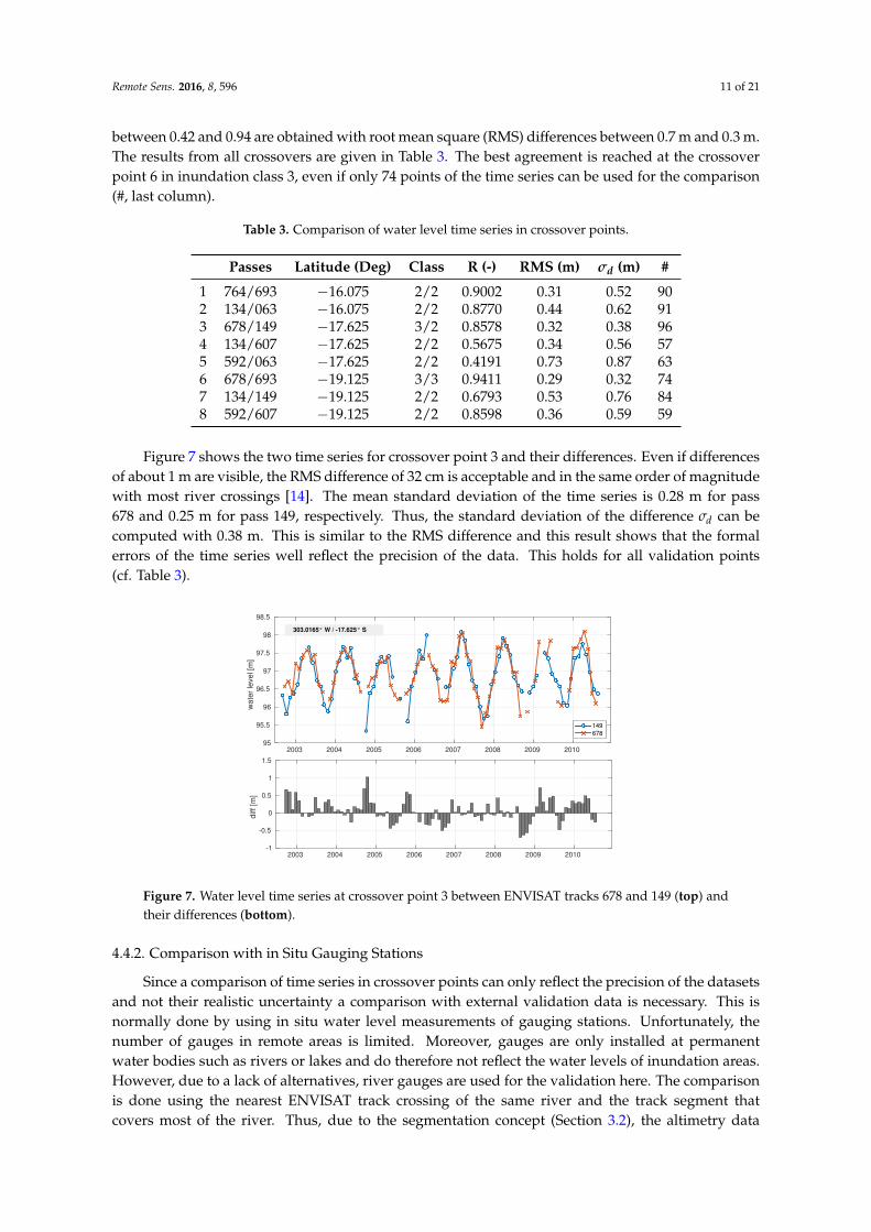
between 0.42 and 0.94 are obtained with root mean square (RMS) differences between 0.7 m and 0.3 m.The results from all crossovers are given in Table 3. The best agreement is reached at the crossoverpoint 6 in inundation class 3, even if only 74 points of the time series can be used for the comparison(#, last column).
Table 3. Comparison of water level time series in crossover points.
Passes Latitude (Deg) Class R (-) RMS (m) σd (m) #
1 764/693 −16.075 2/2 0.9002 0.31 0.52 902 134/063 −16.075 2/2 0.8770 0.44 0.62 913 678/149 −17.625 3/2 0.8578 0.32 0.38 964 134/607 −17.625 2/2 0.5675 0.34 0.56 575 592/063 −17.625 2/2 0.4191 0.73 0.87 636 678/693 −19.125 3/3 0.9411 0.29 0.32 747 134/149 −19.125 2/2 0.6793 0.53 0.76 848 592/607 −19.125 2/2 0.8598 0.36 0.59 59
Figure 7 shows the two time series for crossover point 3 and their differences. Even if differencesof about 1 m are visible, the RMS difference of 32 cm is acceptable and in the same order of magnitudewith most river crossings [14]. The mean standard deviation of the time series is 0.28 m for pass678 and 0.25 m for pass 149, respectively. Thus, the standard deviation of the difference σd can becomputed with 0.38 m. This is similar to the RMS difference and this result shows that the formalerrors of the time series well reflect the precision of the data. This holds for all validation points(cf. Table 3).
2003 2004 2005 2006 2007 2008 2009 2010
wa
ter
leve
l [m
]
95
95.5
96
96.5
97
97.5
98
98.5
149
678
2003 2004 2005 2006 2007 2008 2009 2010
diff
[m]
-1
-0.5
0
0.5
1
1.5
303.0165° W / -17.625° S
Figure 7. Water level time series at crossover point 3 between ENVISAT tracks 678 and 149 (top) andtheir differences (bottom).
4.4.2. Comparison with in Situ Gauging Stations
Since a comparison of time series in crossover points can only reflect the precision of the datasetsand not their realistic uncertainty a comparison with external validation data is necessary. This isnormally done by using in situ water level measurements of gauging stations. Unfortunately, thenumber of gauges in remote areas is limited. Moreover, gauges are only installed at permanentwater bodies such as rivers or lakes and do therefore not reflect the water levels of inundation areas.However, due to a lack of alternatives, river gauges are used for the validation here. The comparisonis done using the nearest ENVISAT track crossing of the same river and the track segment thatcovers most of the river. Thus, due to the segmentation concept (Section 3.2), the altimetry data

Remote Sens. 2016, 8, 596 12 of 21
used for processing the time series is not directly located above the river and can also comprise riverfloodplains. Moreover, a validation of time series offside larger rivers is impossible.
Within the Pantanal, data of about 25 river gauging stations are provided by Agencia Nacionalde Aguas [51]. After rejecting all datasets that do not overlap with ENVISAT over more than one yearonly six stations remain in the central area of the Pantanal with measurements starting in 2005. Theyare distributed along three different rivers in the region. Since all six in situ time series are of minorquality (especially in the first years) and show a lot of outliers and unreliable data points a rigorousdata screening is required. This is performed based on daily data sets by means of a 3σ-outlier test(taking annual variations into account) and a manual post-processing. The amount of rejected outliersvaries between 3.5% for station Posada Taiama and 23.8% for Porto Cercado.
Table 4 summarizes the comparison. In addition to information on the gauge (station name,river, and location), the distance to the altimetry target and the ENVISAT track number are provided.A large distance will for sure have a negative influence on the similarity of the time series since theconditions at the two locations cannot assume to be equal. It is worth mentioning, that the distanceis computed from a straight line to the next ENVISAT crossing of the same river. The distance alongthe river will be much longer in most cases. The last three columns of the table show some statisticsfrom the time series comparisons (RMS difference, correlation coefficient R, and number of points forthe comparison). With one exception, the RMS differences are between 30 and 50 cm. These valuesare in the same order of magnitude with the results from the crossover analysis (Section 4.4.1) and theformal errors of the altimetry time series.
Table 4. Comparison of water level time series at in situ stations.
Station River Lon/Lat ENVISAT Distance RMS R #(Deg) Track (km) (m) (-)
Caceres Rio Paraguay −57.7522/−16.0758 149 64 0.49 0.9511 43Porto Cercado Rio Cuiaba −56.3756/−16.5119 607 26 0.40 0.9189 35Sao Jeronimo Rio Piquiri −56.0086/−17.2017 134 17 0.32 0.9388 42Posada Taiama Rio Cuiaba −56.7747/−17.3656 678 31 0.35 0.9487 52Sao Francisco Rio Paraguay −57.3841/−18.3939 693 22 0.29 0.9870 47Ladario Rio Paraguay −57.5942/−19.0017 693 30 0.96 0.8188 31
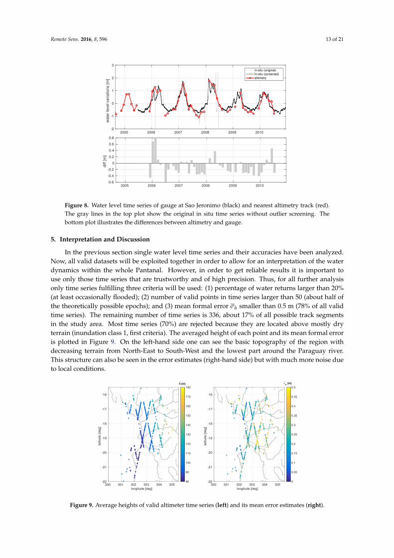
Good agreement between altimetry and in situ data is observed for station Sao Jeronimo at theRio Piquiri. Here, the distance to the nearest altimeter track segment close to the river is around 17 kmupstream. Moreover, there is almost no meander between the two locations and similar conditionscan be assumed. The two time-series are shown in Figure 8.
They have about five years overlapping time for comparison. Since the absolute level of thein situ data is unknown, both time series are reduced by their means and only height variationsare compared. Due to the different temporal resolutions the in situ data were interpolated to thealtimeter time tags and 42 data points are compared. The RMS differences yield 32 cm with the largestdifferences during the low water periods. This is in line with the formal errors of the altimeter timeseries (see Section 4.3). It should be considered, that the altimetry time series is not computed directlyover the river but at the nearest track segment defined in Section 3.2. Thus, they cannot optimallyrepresent the river. This will add an additional error contribution to the uncertainties of water levelmeasurements of altimeter and gauging station. Keeping this in mind, an accuracy of 30 cm is verygood, since it is in the same order of magnitude with results for dedicated river time series [10,14].
In order to evaluate the quality of the water level time series, the RMS should be related to theheight variations itself. In case of larger variations, a higher RMS is acceptable since the variation isstill well depicted. Thus, for the areas with small water level amplitudes of only a few decimeters theaccuracies are within the range of the signal itself. Here, an interpretation of the results is difficult.
Remote Sens. 2016, 8, 596 13 of 21
2005 2006 2007 2008 2009 2010
wa
ter
leve
l va
ria
tio
ns [
m]
-2
-1
0
1
2
3
in-situ (original)
in-situ (screened)
altimetry
2005 2006 2007 2008 2009 2010
diff
[m]
-0.6
-0.4
-0.2
0
0.2
0.4
0.6
0.8
Figure 8. Water level time series of gauge at Sao Jeronimo (black) and nearest altimetry track (red).The gray lines in the top plot show the original in situ time series without outlier screening. Thebottom plot illustrates the differences between altimetry and gauge.
5. Interpretation and Discussion
In the previous section single water level time series and their accuracies have been analyzed.Now, all valid datasets will be exploited together in order to allow for an interpretation of the waterdynamics within the whole Pantanal. However, in order to get reliable results it is important touse only those time series that are trustworthy and of high precision. Thus, for all further analysisonly time series fulfilling three criteria will be used: (1) percentage of water returns larger than 20%(at least occasionally flooded); (2) number of valid points in time series larger than 50 (about half ofthe theoretically possible epochs); and (3) mean formal error σh smaller than 0.5 m (78% of all validtime series). The remaining number of time series is 336, about 17% of all possible track segmentsin the study area. Most time series (70%) are rejected because they are located above mostly dryterrain (inundation class 1, first criteria). The averaged height of each point and its mean formal erroris plotted in Figure 9. On the left-hand side one can see the basic topography of the region withdecreasing terrain from North-East to South-West and the lowest part around the Paraguay river.This structure can also be seen in the error estimates (right-hand side) but with much more noise dueto local conditions.
longitude [deg]
300 301 302 303 304 305
latitu
de
[d
eg
]
-22
-21
-20
-19
-18
-17
-16
h [m]
80
90
100
110
120
130
140
150
160
170
180
longitude [deg]
300 301 302 303 304 305
latitu
de
[d
eg
]
-22
-21
-20
-19
-18
-17
-16
σh
[m]
0
0.05
0.1
0.15
0.2
0.25
0.3
0.35
0.4
0.45
0.5
Figure 9. Average heights of valid altimeter time series (left) and its mean error estimates (right).
Remote Sens. 2016, 8, 596 14 of 21
5.1. Harmonic Fitting
The common interpretation of all time series is demanding since the local conditions differsignificantly from each other and the time series show quite different behavior. In order to analyzethe results the time series are represented by harmonic functions. A fitting by linear or splineinterpolation is not used because they produce unreliable results in the case of data gaps that arefrequent in the time series, especially in areas that are only occasionally flooded.
A Fourier Series is fitted to each time series using Equation (2) with six terms (k = 6), i.e.,13 unknown parameters are estimated representing one constant (describing the mean height), sixamplitudes, and six phases. The fundamental period of the function is fixed to one year (w = 2π) inorder to represent seasonal variations.
f (t) = c +k
∑i=1
ai cos (iwt) + bi sin (iwt) = c +k
∑i=1
Ai cos (iwt + φi) (2)
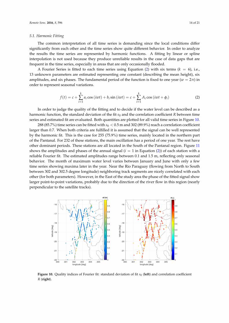
In order to judge the quality of the fitting and to decide if the water level can be described as aharmonic function, the standard deviation of the fit s0 and the correlation coefficient R between timeseries and estimated fit are evaluated. Both quantities are plotted for all valid time series in Figure 10.
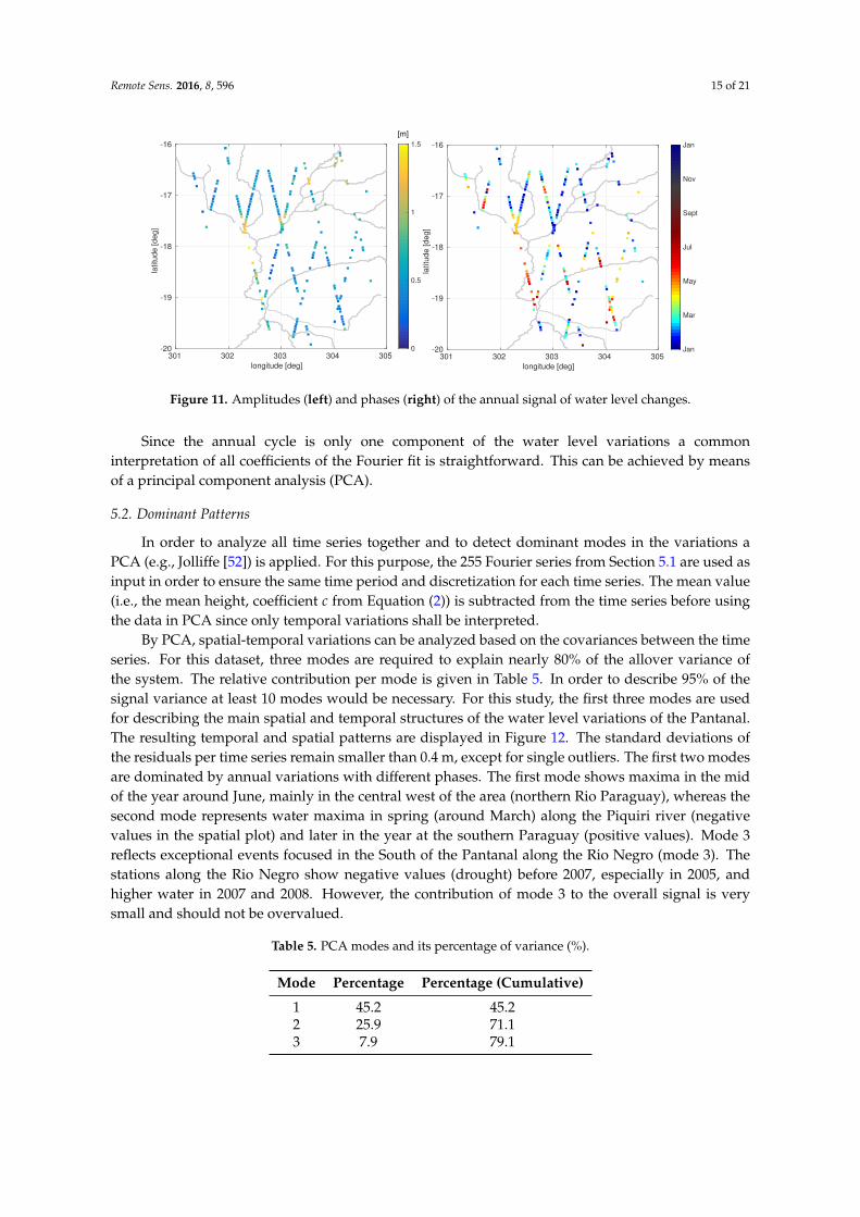
288 (85.7%) time series can be fitted with s0 < 0.5 m and 302 (89.9%) reach a correlation coefficientlarger than 0.7. When both criteria are fulfilled it is assumed that the signal can be well representedby the harmonic fit. This is the case for 255 (75.9%) time series, mainly located in the northern partof the Pantanal. For 232 of these stations, the main oscillation has a period of one year. The rest haveother dominant periods. These stations are all located in the South of the Pantanal region. Figure 11shows the amplitudes and phases of the annual signal (i = 1 in Equation (2)) of each station with areliable Fourier fit. The estimated amplitudes range between 0.1 and 1.5 m, reflecting only seasonalbehavior. The month of maximum water level varies between January and June with only a fewtime series showing maxima later in the year. Near the Rio Paraguay (flowing from North to Southbetween 302 and 302.5 degree longitude) neighboring track segments are nicely correlated with eachother (for both parameters). However, in the East of the study area the phase of the fitted signal showlarger point-to-point variations, probably due to the direction of the river flow in this region (nearlyperpendicular to the satellite tracks).
longitude [deg]
300 301 302 303 304 305
latitu
de [deg]
-22
-21
-20
-19
-18
-17
-16
s0 [m]
0
0.1
0.2
0.3
0.4
0.5
0.6
0.7
0.8
0.9
1
longitude [deg]
300 301 302 303 304 305
latitu
de [deg]
-22
-21
-20
-19
-18
-17
-16
R [-]
0
0.1
0.2
0.3
0.4
0.5
0.6
0.7
0.8
0.9
1
Figure 10. Quality indices of Fourier fit: standard deviation of fit s0 (left) and correlation coefficientR (right).
Remote Sens. 2016, 8, 596 15 of 21
longitude [deg]
301 302 303 304 305
latitu
de [deg]
-20
-19
-18
-17
-16
0
0.5
1
1.5
longitude [deg]
301 302 303 304 305
latitu
de [deg]
-20
-19
-18
-17
-16
Jan
Mar
May
Jul
Sept
Nov
Jan
[m]
Figure 11. Amplitudes (left) and phases (right) of the annual signal of water level changes.
Since the annual cycle is only one component of the water level variations a commoninterpretation of all coefficients of the Fourier fit is straightforward. This can be achieved by meansof a principal component analysis (PCA).
5.2. Dominant Patterns
In order to analyze all time series together and to detect dominant modes in the variations aPCA (e.g., Jolliffe [52]) is applied. For this purpose, the 255 Fourier series from Section 5.1 are used asinput in order to ensure the same time period and discretization for each time series. The mean value(i.e., the mean height, coefficient c from Equation (2)) is subtracted from the time series before usingthe data in PCA since only temporal variations shall be interpreted.
By PCA, spatial-temporal variations can be analyzed based on the covariances between the timeseries. For this dataset, three modes are required to explain nearly 80% of the allover variance ofthe system. The relative contribution per mode is given in Table 5. In order to describe 95% of thesignal variance at least 10 modes would be necessary. For this study, the first three modes are usedfor describing the main spatial and temporal structures of the water level variations of the Pantanal.The resulting temporal and spatial patterns are displayed in Figure 12. The standard deviations ofthe residuals per time series remain smaller than 0.4 m, except for single outliers. The first two modesare dominated by annual variations with different phases. The first mode shows maxima in the midof the year around June, mainly in the central west of the area (northern Rio Paraguay), whereas thesecond mode represents water maxima in spring (around March) along the Piquiri river (negativevalues in the spatial plot) and later in the year at the southern Paraguay (positive values). Mode 3reflects exceptional events focused in the South of the Pantanal along the Rio Negro (mode 3). Thestations along the Rio Negro show negative values (drought) before 2007, especially in 2005, andhigher water in 2007 and 2008. However, the contribution of mode 3 to the overall signal is verysmall and should not be overvalued.
Table 5. PCA modes and its percentage of variance (%).
Mode Percentage Percentage (Cumulative)
1 45.2 45.22 25.9 71.13 7.9 79.1

Remote Sens. 2016, 8, 596 16 of 21
Figure 12. First three modes of PCA. Left-hand side: Principal Components (PC) representingthe temporal patterns; right-hand side: Empirical Orthogonal Functions (EOF) showing the spatialpatterns of water level variations.
5.3. Comparison with Mass Changes Derived from Gravity Recovery and Climate Experiment(GRACE) Mission
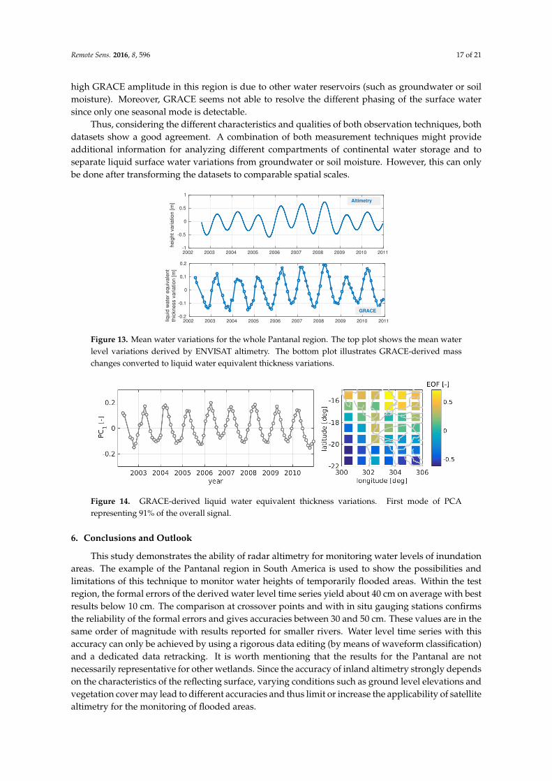
In order to evaluate the altimetry-derived water level changes they are compared to masschanges observed by the GRACE mission [53]. Monthly GRACE gridded land fields [54] are usedto compare liquid water equivalent thickness (LWE) variations with water level variations. Theresults are based on the solution of GFZ (Deutsches Geoforschungszentrum). However, no significantdifferences can be seen when analyzing one of the other two solutions. Figure 13 shows thealtimetry-derived water level variations (top) and the GRACE-derived LWE (bottom) for the wholestudy area. The first plot is computed by averaging all time series from Section 5.2 (as used forPCA). Both time series shows similar variations with a clear seasonality. For the years 2006 to 2008larger amplitudes can be seen in both time series. The correlation coefficient R yields 0.95. However,the absolute amplitudes differ by a factor of about two. This may be related to two main facts:(1) the altimetry time series do not represent the whole area as they are only provided at dedicatedstations; and (2) the GRACE time series is smoothed due to the data sampling and post-processing(e.g., de-striping and filtering) even though the recommended scale factor is applied. Moreover, themeasured quantities of the two time series are not directly comparable: GRACE observes total masschanges whereas altimetry can only measure surface waters. Thus, a reasonable comparison is onlypossible on a relative level without taking the absolute values into account.
In a next step, a PCA is applied to the GRACE dataset (given on a 1-degree grid) in orderto analyze the spatial variability of the data. Figure 14 illustrates the result. The first PCA moderepresents 90.8% of the signal, thus, all further modes are negligible and will not be interpreted.Comparing the spatial pattern to the altimetry result (Figure 12) one can detect some congruences.The largest GRACE amplitudes can be seen in the northern part of the region and along the RiverParaguay. This also holds for altimetry even though separated to different modes: mode 1 showsthe largest amplitudes along the Paraguay and mode 2 in the northeast (Rio Cuiaba). However,the altimetry results indicate higher water level variations along the Paraguay than along the RioCuiaba. Moreover, only moderate amplitudes are visible in the north and northwest. Probably, the
Remote Sens. 2016, 8, 596 17 of 21
high GRACE amplitude in this region is due to other water reservoirs (such as groundwater or soilmoisture). Moreover, GRACE seems not able to resolve the different phasing of the surface watersince only one seasonal mode is detectable.
Thus, considering the different characteristics and qualities of both observation techniques, bothdatasets show a good agreement. A combination of both measurement techniques might provideadditional information for analyzing different compartments of continental water storage and toseparate liquid surface water variations from groundwater or soil moisture. However, this can onlybe done after transforming the datasets to comparable spatial scales.
2002 2003 2004 2005 2006 2007 2008 2009 2010 2011
he
igh
t va
ria
tio
n [
m]
-1
-0.5
0
0.5
1
2002 2003 2004 2005 2006 2007 2008 2009 2010 2011liqu
id w
ate
r e
qu
iva
len
t
thic
kn
ess v
aria
tio
n [
m]
-0.2
-0.1
0
0.1
0.2
Altimetry
GRACE
Figure 13. Mean water variations for the whole Pantanal region. The top plot shows the mean waterlevel variations derived by ENVISAT altimetry. The bottom plot illustrates GRACE-derived masschanges converted to liquid water equivalent thickness variations.
Figure 14. GRACE-derived liquid water equivalent thickness variations. First mode of PCArepresenting 91% of the overall signal.
6. Conclusions and Outlook
This study demonstrates the ability of radar altimetry for monitoring water levels of inundationareas. The example of the Pantanal region in South America is used to show the possibilities andlimitations of this technique to monitor water heights of temporarily flooded areas. Within the testregion, the formal errors of the derived water level time series yield about 40 cm on average with bestresults below 10 cm. The comparison at crossover points and with in situ gauging stations confirmsthe reliability of the formal errors and gives accuracies between 30 and 50 cm. These values are in thesame order of magnitude with results reported for smaller rivers. Water level time series with thisaccuracy can only be achieved by using a rigorous data editing (by means of waveform classification)and a dedicated data retracking. It is worth mentioning that the results for the Pantanal are notnecessarily representative for other wetlands. Since the accuracy of inland altimetry strongly dependson the characteristics of the reflecting surface, varying conditions such as ground level elevations andvegetation cover may lead to different accuracies and thus limit or increase the applicability of satellitealtimetry for the monitoring of flooded areas.

Remote Sens. 2016, 8, 596 18 of 21
Due to its measurement geometry along dedicated satellite ground tracks, satellite altimetryis not able to provide a complete data coverage of the Pantanal. Even though a high along-trackresolution of a few km is possible, the cross-track resolution depends on the orbit of the mission(s)used. This study is limited to ENVISAT data. The use of additional missions such as Jason-2 orSentinel-3 might improve the spatial (and temporal) data coverage. Of course, altimetry can onlyprovide water levels if the area within the footprint is partly covered by water – at least for a certainperiod of time.
Since it is not possible to use a constant land-water mask to define flooded areas, externaldatasets are necessary. This study uses the altimetry returns themselves to identify open waterreturns: waveform classification or backscatter analysis show similar results and are both suitable forthis purpose. A separation of the Pantanal in four inundation classes based on altimeter waveformclassification shows a good agreement to classifications based on imaging data (GIEMS-D15).
Using altimetry, seasonal water level variations as well as particular events can be detected. Itallows for analyzing floods in space and time. For the Pantanal, most areas show a clear annualcycle with maximum water levels between January (north/east of the region) and June (south). Theamplitudes can reach up to about 1.5 m for larger rivers and their floodplains. However, substantialareas of the Pantanal show smaller water level variations (only a few decimeters), which are in thesame order of magnitude with the accuracies of inland radar altimetry. For these parts of the Pantanal,no reliable water height information is extractable. Further investigations are necessary to improvethe results in these areas. The usage of delay-doppler altimeter data (such as measured by the recentlylaunched Sentinel-3 mission) might improve the along-track resolution and the extraction of waterreturns in vegetated areas.
A combination of altimeter-derived water levels with surface water extent from imaging sensorsor databases will enable to estimate water storage and its variations solely based on remote sensingdata. These information are very valuable for understanding the continental and global watercycle. This metric on water storage within the flooded area may be interpreted together withGRACE-derived mass changes and other external data (such as precipitation and evaporation) inorder to derive and evaluate hydrological water balances.
Acknowledgments: The authors thank the following people and institutions for providing data and models:ESA for operating the ENVISAT mission and for disseminates the SGDR datasets. E. Fluet-Chouinard et al.for developing and providing the GIEMS-D15 model. U.S. Geological Survey (USGS) and World WildlifeFund (WWF) for providing HydroSHEDS [42,55]. Agencia Nacional de Aguas [51] for providing the in situgauging datasets. GRACE Tellus Level-3 gridded land fields are available at PODAAC [54], supported by theNASA MEaSUREs Program. Moreover, we want to thank Anne Braakmann-Folkmann for her contributionto the early stage of the study. This study is part of the project WLDYN that is funded by the DeutscheForschungsgemeinschaft DFG, grant SE1916/4-1. We thank four anonymous reviewers for their valuablecomments that helped to improve the manuscript.
Author Contributions: Denise Dettmering led the study, computed the water level time series, analyzed thedata and wrote the majority of the paper. Christian Schwatke developed the waveform classification and codedthe altimeter retracker; Eva Boergens, Christian Schwatke, and Florian Seitz helped with discussions on themethod and results. All authors contributed to the writing of the manuscript.
Conflicts of Interest: The authors declare no conflict of interest.
References
1. Fu, L.L.; Cazenave, A. Satellite Altimetry and Earth Sciences: A Handbook of Techniques and Applications;International Geophysics Series; Academic Press: Waltham, MA, USA, 2001.
2. Ablain, M.; Cazenave, A.; Larnicol, G.; Balmaseda, M.; Cipollini, P.; Faugere, Y.; Fernandes, M.J.; Henry, O.;Johannessen, J.A.; Knudsen, P.; et al. Improved sea level record over the satellite altimetry era (1993–2010)from the Climate Change Initiative project. Ocean Sci. 2015, 11, 67–82.
3. Woodworth, P.L.; Menendez, M. Changes in the mesoscale variability and in extreme sea levels over twodecades as observed by satellite altimetry. J. Geophys. Res. 2015, 120, 64–77.

Remote Sens. 2016, 8, 596 19 of 21
4. Davis, C.H.; Ferguson, A.C. Elevation change of the Antarctic ice sheet, 1995–2000, from ERS-2 satelliteradar altimetry. IEEE Trans. Geosci. Remote Sens. 2004, 42, 2437–2445.
5. Berry, P.A.M.; Garlick, J.D.; Freeman, J.A.; Mathers, E.L. Global inland water monitoring frommulti-mission altimetry. Geophys. Res. Lett. 2005, 32, doi:10.1029/2005GL022814.
6. Crétaux, J.F.; Birkett, C. Lake studies from satellite radar altimetry. Comptes Rendus Geosci. 2006,338, 1098–1112.
7. Uebbing, B.; Kusche, J.; Forootan, E. Waveform retracking for improving level estimations fromTOPEX/Poseidon, Jason-1, and Jason-2 altimetry observations over African lakes. IEEE Trans. Geosci.Remote Sens. 2015, 53, 2211–2224.
8. Santos da Silva, J.; Calmant, S.; Seyler, F.; Rotunno Filho, O.C.; Cochonneau, G.; Mansur, W.J.J. Water levelsin the Amazon basin derived from the ERS 2 and ENVISAT radar altimetry missions. Remote Sens. Environ.2010, 114, 2160–2181.
9. Becker, M.; da Silva, J.S.; Calmant, S.; Robinet, V.; Linguet, L.; Seyler, F. Water level fluctuations in theCongo Basin derived from ENVISAT satellite altimetry. Remote Sens. 2014, 6, 9340–9358.
10. Boergens, E.; Dettmering, D.; Schwatke, C.; Seitz, F. Treating the hooking effect in satellite altimetry data:A case study along the Mekong River and its tributaries. Remote Sens. 2016, 8, 91.
11. Berry, P.; Wheeler, J. Development of Algorithms for the Exploitation of JASON2-ENVISAT Altimetry for theGeneration of a River and Lake Product; Product Handbook 3.05 Internal Report DMU-RIVL-SPE-03-110,ESA; De Montfort University: Leicester, UK, 2009.
12. Birkett, C.M.; Reynolds, C.; Beckley, B.; Doorn, B. From research to operations: The USDA global reservoirand lake monitor. In Coastal Altimetry; Vignudelli, S., Kostianoy, A.G., Cipollini, P., Benveniste, J., Eds.;Springer: Berlin, Germany; Heidelberg, Germany, 2011; pp. 19–50.
13. Crétaux, J.F.; Jelinski, W.; Calmant, S.; Kouraev, A.; Vuglinski, V.; Bergé-Nguyen, M.; Gennero, M.C.;Nino, F.; Rio, R.A.D.; Cazenave, A.; et al. SOLS: A lake database to monitor in the Near Real Time waterlevel and storage variations from remote sensing data. Adv. Space Res. 2011, 47, 1497–1507.
14. Schwatke, C.; Dettmering, D.; Bosch, W.; Seitz, F. DAHITI—An innovative approach for estimating waterlevel time series over inland waters using multi-mission satellite altimetry. Hydrol. Earth Syst. Sci. 2015,19, 4345–4364.
15. GRDC. Global Runoff Data Base—Statistics 2013.16. Chelton, D.; Ries, J.; Haines, B.; Fu, L.L.; Callahan, P. Satellite Altimetry and Earth Sciences. A Handbook of
Techniques and Applications; Academic Press: Waltham, MA, USA, 2001; Chapter Satellite Altimetry.17. Papa, F.; Legrésy, B.; Rémy, F. Use of the Topex–Poseidon dual-frequency radar altimeter over land surfaces.
Remote Sens. Environ. 2003, 87, 136–147.18. Le, Y.; Qinhuo, L.; Jing, Z.; Lifeng, B. Global Land Surface Backscatter at Ku-Band Using Merged Jason1,
Envisat, and Jason2 Data Sets. IEEE Trans. Geosci. Remote Sens. 2015, 53, 784–794.19. Smith, R.; Berry, P. Contribution to wetland monitoring of multi-mission satellite radar altimetry. In
Proceedings of the Hydrospace07 Workshop, Geneva, Switzerland, 12–14 November 2007.20. Lee, H.; Shum, C.K.; Yi, Y.; Ibaraki, M.; Kim, J.W.; Braun, A.; Kuo, C.Y.; Lu, Z. Louisiana Wetland Water
Level Monitoring Using Retracked TOPEX/POSEIDON Altimetry. Mar. Geodesy 2009, 32, 284–302.21. Khajeh, S.; Jazireeyan, I.; Ardalan, A. Applying Satellite Altimetry to Wetland Water Levels Monitoring
(Case Study: Louisiana Wetland). IEEE Geosci. Remote Sens. Lett. 2014, 11, 1475–1478.22. Cai, X.; Ji, W. Wetland hydrologic application of satellite altimetry—A case study in the Poyang Lake
watershed. Progr. Natural Sci. 2009, 19, 1781–1787.23. Birkett, C.M.; Mertes, L.A.K.; Dunne, T.; Costa, M.H.; Jasinski, M.J. Surface water dynamics in the Amazon
Basin: Application of satellite radar altimetry. J. Geophys. Res. Atmos. 2002, 107, LBA 26–1–LBA 26–21.24. Frappart, F.; Seyler, F.; Martinez, J.M.; León, J.G.; Cazenave, A. Floodplain water storage in the Negro River
basin estimated from microwave remote sensing of inundation area and water levels. Remote Sens. Environ.2005, 99, 387–399.
25. Zakharova, E.A.; Kouraev, A.V.; Rémy, F.; Zemtsov, V.A.; Kirpotin, S.N. Seasonal variability of the WesternSiberia wetlands from satellite radar altimetry. J. Hydrol. 2014, 512, 366–378.
26. Papa, F.; Prigent, C.; Rossow, W.B.; Legresy, B.; Remy, F. Inundated wetland dynamics over boreal regionsfrom remote sensing: The use of Topex-Poseidon dual-frequency radar altimeter observations. Int. J.Remote Sens. 2006, 27, 4847–4866.
Remote Sens. 2016, 8, 596 20 of 21
27. Hamilton, S.K.; Sippel, S.J.; Melack, J.M. Inundation patterns in the Pantanal wetland of South Americadetermined from passive microwave remote sensing. Arch. Hydrobiol. 1996, 137, 1–23.
28. Hamilton, S.K.; Sippel, S.J.; Melack, J.M. Comparison of inundation patterns among major South Americanfloodplains. J. Geophys. Res. Atmos. 2002, 107, LBA 5:1–LBA 5:14.
29. Evans, T.L.; Costa, M.; Silva, T.; Telmer, K. Using PALSAR and RADARSAT-2 to map land cover andinundation in the Brazilian Pantanal. In Proceedings of the 3o Simpósio de Geotecnologias no Pantanal,Caceres, Brazil, 16–20 October 2010; pp. 485–494.
30. Evans, T.L.; Costa, M. Landcover classification of the Lower Nhecolândia subregion of the BrazilianPantanal Wetlands using ALOS/PALSAR, RADARSAT-2 and ENVISAT/ASAR imagery. Remote Sens.Environ. 2013, 128, 118–137.
31. Girard, P.; Fantin-Cruz, I.; de Oliveira, S.; Hamilton, S. Small-scale spatial variation of inundation dynamicsin a floodplain of the Pantanal (Brazil). Hydrobiologia 2010, 638, 223–233.
32. Padovani, C. Dinamica Espaco-Temporal das Inundacoes do Pantanal. Ph.D. Thesis, Escola Superiorde Agricultura “Luiz de Queiroz”, Centro de Energia Nuclear na Agricultura, University of Sao Paulo,Sao Paulo, Brazil, 2010.
33. Hamilton, S.K. Hydrological controls of ecological structure and function in the Pantanal wetland (Brazil).In The Ecohydrology of South American Rivers and Wetlands; IAHS Special Publication: Wallingford, UK, 2002.
34. ESA. ENVISAT RA2/MWR Product Handbook; Technical Report Issue 2.2; ESA: Paris, France, 2007.35. Bosch, W.; Dettmering, D.; Schwatke, C. Multi-Mission Cross-Calibration of Satellite Altimeters:
Constructing a Long-Term Data Record for Global and Regional Sea Level Change Studies. Remote Sens.2014, 6, 2255–2281.
36. Förste, C.; Bruinsma, S.; Flechtner, F.; Marty, J.; Lemoine, J.; Dahle, C.; Abrikosov, O.; Neumayer, H.;Biancale, R.; Barthelmes, F.; et al. A new release of EIGEN-6C. In Proceedings of the AGU Fall Meeting2012, San Francisco, CA, USA, 3–7 December 2012.
37. Amante, C.; Eakins, B. ETOPO1 1 Arc-Minute Global Relief Model: Procedures, Data Sources and Analysis;NOAA Technical Memorandum NESDIS NGDC-24; National Geophysical Data Center, NOAA: Boulder,CO, USA, 2009.
38. Boehm, J.; Kouba, J.; Schuh, H. Forecast Vienna Mapping Functions 1 for real-time analysis of spacegeodetic observations. J. Geodesy 2009, 83, 397–401.
39. Scharroo, R.; Smith, W.H.F. A global positioning system-based climatology for the total electron content inthe ionosphere. J. Geophys. Res. 2010, 115, 16.
40. McCarthy, D.D.; Petit, G. Eds. IERS Conventions (2003); IERS Technical Note 32; Verlag des Bundesamts fürKartographie und Geodäsie: Frankfurt am Main, Germany, 2004.
41. Desai, S.; Chander, S.; Ganguly, D.; Chauhan, P.; Lele, P.D.; James, M.E. Waveform Classification andWater-Land Transition over the Brahmaputra River using SARAL/AltiKa & Jason-2 Altimeter. J. IndianSoc. Remote Sens. 2015, 43, 475–485.
42. Lehner, B.; Verdin, K.; Jarvis, A. New Global Hydrography Derived From Spaceborne Elevation Data. EosTrans. Am. Geophys. Union 2008, 89, 93.
43. Wessel, P.; Smith, W.H.F. Free software helps map and display data. Eos Trans. Am. Geophys. Union 1991,72, 441–446.
44. U.S. EPA. Methods for Evaluating Wetland Condition: Wetland Hydrology; Technical Report EPA-822-R-08-024;Office of Water, U.S. Environmental Protection Agency (EPA): Washington, DC, USA, 2008.
45. Fluet-Chouinard, E.; Lehner, B.; Rebelo, L.M.; Papa, F.; Hamilton, S.K. Development of a global inundationmap at high spatial resolution from topographic downscaling of coarse-scale remote sensing data. RemoteSens. Environ. 2015, 158, 348–361.
46. Prigent, C.; Papa, F.; Aires, F.; Rossow, W.B.; Matthews, E. Global inundation dynamics inferred frommultiple satellite observations, 1993–2000. J. Geophys. Res. 2007, 112, D12107.
47. Moraes, E.C.; Pereira, G.; Cardoso, F.D.S. Evaluation of reduction of Pantanal wetlands in 2012. Geografia2013, 38, 81–94.
48. Frappart, F.; Calmant, S.; Cauhopé, M.; Seyler, F.; Cazenave, A. Preliminary results of ENVISATRA-2-derived water levels validation over the Amazon basin. Remote Sens. Environ. 2006, 100, 252–264.
Remote Sens. 2016, 8, 596 21 of 21
49. Crétaux, J.F.; Calmant, S.; Romanovski, V.; Shabunin, A.; Lyard, F.; Bergé-Nguyen, M.; Cazenave, A.;Hernandez, F.; Perosanz, F. An absolute calibration site for radar altimeters in the continental domain:Lake Issykkul in Central Asia. J. Geodesy 2009, 83, 723–735.
50. Hwang, C.; Guo, J.; Deng, X.; Hsu, H.Y.; Liu, Y. Coastal Gravity Anomalies from Retracked Geosat/GMAltimetry: Improvement, Limitation and the Role of Airborne Gravity Data. J. Geodesy 2006, 80, 204–216.
51. ANA. National Water Agency. Available online: http://ana.gov.br (accessed on 12 July 2016).52. Jolliffe, I.T. Principal Component Analysis, Second Edition; Springer: Berlin, Germany, 2002.53. Tapley, B.D.; Bettadpur, S.; Watkins, M.; Reigber, C. The gravity recovery and climate experiment: Mission
overview and early results. Geophys. Res. Lett. 2004, 31.54. Swenson, S. GRACE Monthly Land Water Mass Grids NETCDF RELEASE 5.0. Ver. 5.0. PO.DAAC, CA,
USA. Available online: http://dx.doi.org/10.5067/TELND-NC005 (accessed on 21 April 2016).55. HydroSHEDS. Hydrological Data and Maps Based on Shuttle Elevation Derivatives at Multiple Scales.
Available online: http://hydrosheds.cr.usgs.gov (accessed on 12 July 2016).
c© 2016 by the authors; licensee MDPI, Basel, Switzerland. This article is an open accessarticle distributed under the terms and conditions of the Creative Commons Attribution(CC-BY) license (http://creativecommons.org/licenses/by/4.0/).