Potential impacts of electric vehicles on air quality and

Potential impacts of electric vehicles on air quality and health endpoints in the Greater Houston Area in 2040

Center for Transportation, Environment, and Community Health Final Report

by Shuai Pan, H. Oliver Gao

December 30, 2019

DISCLAIMER The contents of this report reflect the views of the authors, who are responsible for the facts and the accuracy of the information presented herein. This document is disseminated in the interest of information exchange. The report is funded, partially or entirely, by a grant from the U.S. Department of Transportation’s University Transportation Centers Program. However, the U.S. Government assumes no liability for the contents or use thereof.

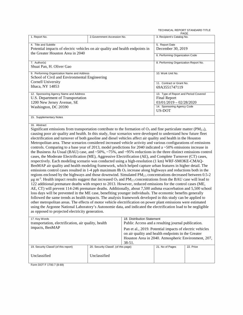
TECHNICAL REPORT STANDARD TITLE PAGE

1. Report No. 2.Government Accession No. 3. Recipient’s Catalog No. 4. Title and Subtitle 5. Report Date Potential impacts of electric vehicles on air quality and health endpoints in the Greater Houston Area in 2040

December 30, 2019 6. Performing Organization Code

7. Author(s) 8. Performing Organization Report No. Shuai Pan, H. Oliver Gao

9. Performing Organization Name and Address 10. Work Unit No. School of Civil and Environmental Engineering Cornell University Ithaca, NY 14853

11. Contract or Grant No. 69A3551747119

12. Sponsoring Agency Name and Address 13. Type of Report and Period Covered U.S. Department of Transportation 1200 New Jersey Avenue, SE Washington, DC 20590

Final Report 03/01/2019 – 02/28/2020 14. Sponsoring Agency Code US-DOT

15. Supplementary Notes 16. Abstract Significant emissions from transportation contribute to the formation of O3 and fine particulate matter (PM2.5), causing poor air quality and health. In this study, four scenarios were developed to understand how future fleet electrification and turnover of both gasoline and diesel vehicles affect air quality and health in the Houston Metropolitan area. These scenarios considered increased vehicle activity and various configurations of emissions controls. Comparing to a base year of 2013, model predictions for 2040 indicated a ~50% emissions increase in the Business As Usual (BAU) case, and ~50%, ~75%, and ~95% reductions in the three distinct emissions control cases, the Moderate Electrification (ME), Aggressive Electrification (AE), and Complete Turnover (CT) cases, respectively. Each modeling scenario was conducted using a high-resolution (1 km) WRF-SMOKE-CMAQ-BenMAP air quality and health modeling framework, which helped capture urban features in higher detail. The emissions control cases resulted in 1-4 ppb maximum 8h O3 increase along highways and reductions both in the regions enclosed by the highways and those downwind. Simulated PM2.5 concentrations decreased between 0.5-2 μg m-3. Health impact results suggest that increased O3 and PM2.5 concentrations from the BAU case will lead to 122 additional premature deaths with respect to 2013. However, reduced emissions for the control cases (ME, AE, CT) will prevent 114-246 premature deaths. Additionally, about 7,500 asthma exacerbation and 5,500 school loss days will be prevented in the ME case, benefiting younger individuals. The economic benefits generally followed the same trends as health impacts. The analysis framework developed in this study can be applied to other metropolitan areas. The effects of motor vehicle electrification on power plant emissions were estimated using the Argonne National Laboratory’s Autonomie data, and indicated the electrification load to be negligible as opposed to projected electricity generation. 17. Key Words 18. Distribution Statement transportation, electrification, air quality, health impacts, BenMAP

Public Access and a resulting journal publication.

Pan et al., 2019. Potential impacts of electric vehicles on air quality and health endpoints in the Greater Houston Area in 2040. Atmospheric Environment, 207, 38-51.

19. Security Classif (of this report) 20. Security Classif. (of this page) 21. No of Pages 22. Price

Unclassified Unclassified

Form DOT F 1700.7 (8-69)

4

Potential impacts of electric vehicles on air quality and health

endpoints in the Greater Houston Area in 2040

Abstract

Significant emissions from transportation contribute to the formation of O3 and fine particulate

matter (PM2.5), causing poor air quality and health. In this study, four scenarios were developed to

understand how future fleet electrification and turnover of both gasoline and diesel vehicles affect air

quality and health in the Houston Metropolitan area. These scenarios considered increased vehicle

activity and various configurations of emissions controls. Comparing to a base year of 2013, model

predictions for 2040 indicated a ~50% emissions increase in the Business As Usual (BAU) case, and

~50%, ~75%, and ~95% reductions in the three distinct emissions control cases, the Moderate

Electrification (ME), Aggressive Electrification (AE), and Complete Turnover (CT) cases, respectively.

Each modeling scenario was conducted using a high-resolution (1 km) WRF-SMOKE-CMAQ-BenMAP

air quality and health modeling framework, which helped capture urban features in higher detail. The

emissions control cases resulted in 1-4 ppb maximum 8h O3 increase along highways and reductions

both in the regions enclosed by the highways and those downwind. Simulated PM2.5 concentrations

decreased between 0.5-2 μg m-3. Health impact results suggest that increased O3 and PM2.5

concentrations from the BAU case will lead to 122 additional premature deaths with respect to 2013.

However, reduced emissions for the control cases (ME, AE, CT) will prevent 114-246 premature deaths.

Additionally, about 7,500 asthma exacerbation and 5,500 school loss days will be prevented in the ME

case, benefiting younger individuals. The economic benefits generally followed the same trends as

health impacts. The analysis framework developed in this study can be applied to other metropolitan

areas. The effects of motor vehicle electrification on power plant emissions were estimated using the

Argonne National Laboratory’s Autonomie data, and indicated the electrification load to be negligible as

opposed to projected electricity generation.

Keywords: transportation, electrification, air quality, health impacts, BenMAP, WRF-SMOKE-CMAQ

1. Introduction

Estimating transportation emissions trends and associated air quality impacts can provide

important insights for requisite control policy. The transportation sector is a major contributor to the

concentrations of both nitrogen oxides (NOx) and volatile organic compounds (VOCs), which react in

the presence of sunlight to form ozone (O3). Vehicular traffic also emits important components of fine

particulate matter (PM2.5) such as organic and elemental carbon (Roy et al., 2011; U.S. EPA, 2017a).

Both O3 and PM2.5 are known to be harmful to human health, causing premature deaths (Bell et al.,

2005; Krewski et al., 2009) and severe and minor morbidities (e.g., hospital admissions and asthma

exacerbations) (Katsouyanni et al., 2009; Mortimer et al., 2002). The adoption of electric vehicles can

lead to significant emissions reductions in the transportation sector (Huo et al., 2012; Nichols et al.,

2015). As of 2017, electric vehicles accounted for ~1% of new car sales in the United States (and much

5

higher in other markets, such as Norway with nearly 30% market share) (Vaughan, 2017). A Bloomberg

New Energy Finance report (BNEF, 2016) estimated that 35% of global new car sales would be electric-

powered in 2040, that was adjusted to 54% in 2017 considering falling battery costs and possible

consumer adoption growth (BNEF, 2017). Policymakers from several countries have announced their

commitments of a transition to electric vehicles. For example, Norway has called for all new car sales to

be electric by 2025; France, the U.K., and the state of California set goals to achieve the same by 2040;

and China aims to electrify 20% of its new cars by 2025 (Walsh, 2017). The implementation of these

policies will have large impact on transportation emissions, air quality, and human health.

Several previous studies have assessed the potential impacts of electric vehicles on air quality in

various regions. Thompson et al. (2009) found that replacing 20% of the gasoline vehicles with electric

vehicles over the northeastern U.S. could reduce MDA8 O3 by 2-6 ppb, barring a few episodes of

significant O3 increases around Newark and Philadelphia. Brinkman et al. (2010) reported that 100%

penetration of electric vehicles in Denver would lower the summertime MDA8 O3 by 2-3 ppb, excluding

a 1-2 ppb increase over the downtown area. Li et al. (2016) reported that fully electrifying all light-duty

vehicles would lead to reductions in MDA8 O3 of 1-2 ppb and mean peak-time O3 of as much as 7 ppb

across Taiwan, except in central metropolitan Taipei (an increase of < 2 ppb). Their findings also

indicated that electrification would reduce the annual number of days of O3 pollution episodes by 40%

and PM2.5 pollution episodes by 6-10%. Nopmongcol et al. (2017) indicated that 17% of light-duty and

8% of heavy-duty vehicle miles traveled and 17-79% of various off-road equipment types would be

targeted for electrification in the U.S. by the year 2030. They reported that electrification would reduce

O3 by less than 1 ppb and PM2.5 by 0.5 µg m-3.

To date, no similar quantitative evaluation has been conducted for the Houston Metropolitan

Area. This is the 4th largest urban area in the United States and classified as a nonattainment area for

ozone (O3) by the United States Environmental Protection Agency (U.S. EPA) (U.S. EPA Green Book,

2017). It is classified as “Marginal” with a current design value (2015-2017) of 80 ppb. It is also in

borderline attainment for fine particulate matter (PM2.5). As indicated by the 2013 Houston Galveston

Area Council (H-GAC) Regional Goods Movement Plan, the population of the Houston area is

projected to grow by 50% in 2040, which will result in increased motor vehicle activity and goods

movement in the region if the projections hold true. Their study also projected a doubling of the number

of trucks in the region by 2040. Another study by the Texas Transportation Institute projected that the

number of trucks in the Houston area would increase by 40%-80% and the number of gasoline vehicles

by 30% to 50% by 2040 (TCEQ, 2015). Thus, the Houston Metropolitan Area provides a valuable

opportunity to evaluate the impact of increased transportation activity and control strategies (e.g., fleet

electrification) on air quality and the subsequent health effects.

In this study, we apply relatively large fleet penetrations of electric vehicles, including a

moderate fraction (35%) and an aggressive one (70%), to on-road mobile source sectors in the Greater

Houston Area for the year 2040. For assessing the future emissions, another important factor that needs

to be considered is fleet turnover, where older motor vehicles are replaced with newer technology,

resulting in a significant reduction in emissions (Roy et al., 2014; Liu et al., 2015). Previous studies have

6

assessed the impact of electrification on transportation emissions (Huo et al., 2012; Nichols et al., 2015)

and air quality (Thompson et al., 2011; Soret et al., 2014; Nopmongcol et al., 2017), but few have

investigated the corresponding health and economic benefits. Pan et al. (2017b) developed and evaluated

a fine-resolution (1×1 km) WRF-SMOKE-CMAQ air quality modeling system to gain an understanding

of the concentrations of O3 and the processes over Houston that drove O3 formation in September 2013.

In this study, we extend this framework by adding a health/benefits model to assess motor vehicle

emissions, fleet electrification and turnover, and their associated air quality and health impacts. This

study aims to answer the following questions:

(1) How would the mobile activity (e.g., vehicle miles traveled) change in the Houston area by 2040?

What are the possible future scenarios corresponding to varying degrees of emission control, fleet

electrification and turnover for gasoline and diesel vehicles? Under these scenarios, how would the

emissions change in 2040?

(2) What are the magnitudes and spatial distributions of changes in regional O3 and its precursors as well

as PM2.5 and its speciated components?

(3) What are the magnitudes of changes in premature mortality, morbidities, and consequent economic

benefits? What are the primary factors affecting the health impact results? How do the health results

vary by county?

2. Methodology

2.1. Air quality modeling system setup and observational data

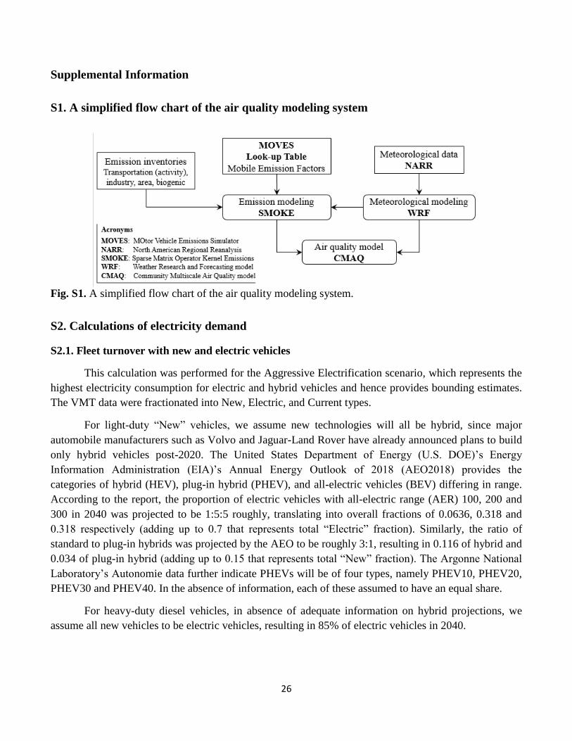
This study employed a WRF-SMOKE-CMAQ modeling system that included meteorological,

emissions, and chemical transport modeling (a simplified flow chart in Fig. S1). Here, we used the U.S.

EPA Community Multi-scale Air Quality (CMAQ) model (Byun and Schere, 2006) version 5.0.2 to

model chemical transport, the Carbon Bond 5 (CB05) (Yarwood et al., 2005) and AERO6 mechanisms

to simulate gas and aerosol chemistry, respectively, and the Weather Research and Forecasting (WRF)

model version 3.7 (Skamarock and Klemp, 2008) to simulate meteorology. This study used the National

Centers for Environmental Prediction (NCEP) North American Regional Reanalysis (NARR) data

(Mesinger et al., 2004) as input for the WRF model. Emission inputs were prepared using the Sparse

Matrix Operator Kernel Emissions (SMOKE) system version 3.6 (Houyoux et al., 2000) using the U.S.

EPA 2011 National Emission Inventory (NEI-2011) (U.S. EPA, 2015a; 2015b). Details of WRF physics

options and CMAQ configurations are listed in Pan et al. (2017b) and used in previous air quality

modeling studies (Li et al., 2016; Pan et al., 2017a).

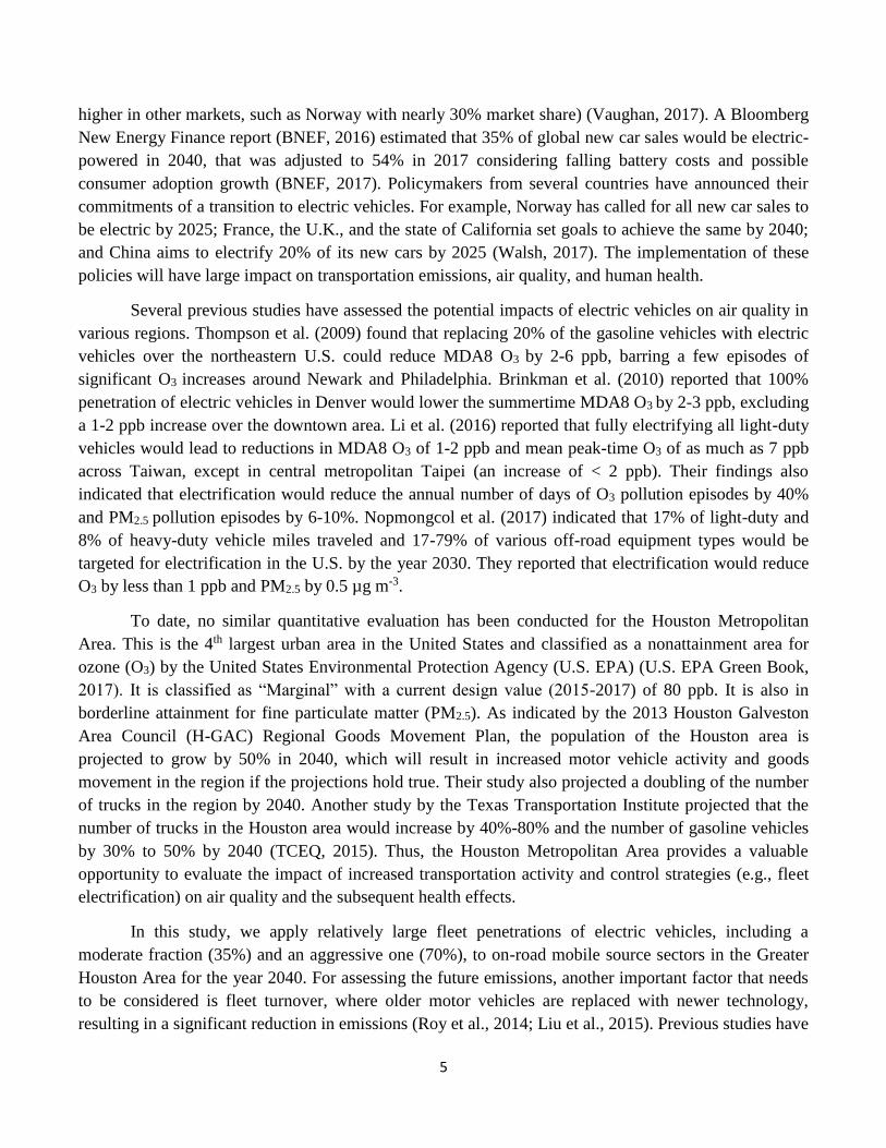
The 1 km resolution simulation domain covered the eight-county Houston-Galveston-Brazoria

(HGB) nonattainment area depicted in Fig. 1. Initial and boundary conditions were obtained from the

Air Quality Forecasting system at the University of Houston (AQF-UH) (http://spock.geosc.uh.edu/,

Choi et al., 2016) over a larger 12 km grid covering the United States, southern Canada, and northern

Mexico (left panel in Fig. 1). Model-measurement evaluation was conducted using the Texas

Commission on Environmental Quality (TCEQ) Continuous Ambient Monitoring Stations (CAMS)

http://spock.geosc.uh.edu/

7

network, which provided in-situ ground-level measurements for several chemical species such as NOx,

O3, and a large suite of VOCs, and the U.S. EPA AirNow network, which provided surface PM2.5

measurements.

Fig. 1. Horizontal domains of WRF and CMAQ at various grid resolutions; the HGB 1 km is used in

this study while the U.S. 12 km is used to provide boundary conditions. In the zoomed-in plot on the

right, roadways are represented in orange and county boundaries in purple.

2.2. Mobile source emissions processing

The air quality simulations in this study used emissions from all major sectors, including mobile,

point, area, and biogenic sectors. Here, the calculations of on-road mobile emissions were specifically

described as we focused on the future change in the transportation sector. This study employed the U.S.

EPA Motor Vehicle Emissions Simulator (MOVES) (U.S. EPA, 2016) and SMOKE models to prepare

on-road mobile emissions. The MOVES model was ran by U.S. EPA to provide emission factors (EF)

look-up tables for mobile emissions as a function of speed, fuel type, vehicle type, road type, and

meteorological conditions. The major fuel types include gasoline and diesel, and the vehicle types

include motorcycle, passenger car/truck, light commercial truck, intercity/transit/school bus, and

medium/heavy duty short-haul/long-haul truck.

In Fig. 2, the “rate-per-distance” (RPD) sector represents on-roadway mobile sources and

emission processes. These emissions are located along the roadway networks inside the simulation

domain. RPD emissions can be calculated using the following simplified formula:

𝐸𝑚𝑖𝑠𝑠𝑖𝑜𝑛𝑅𝑃𝐷 = 𝐸𝐹𝑅𝑃𝐷 × ℎ𝑜𝑢𝑟𝑙𝑦 𝑉𝑀𝑇 (1)

where the unit of 𝐸𝐹𝑅𝑃𝐷 is g mile-1 and 𝑉𝑀𝑇 represents vehicle miles traveled.

The “rate-per-vehicle” (RPV) sector represents off-network mobile emissions, which were

predominantly concentrated in the urban locations and estimated as follows:

𝐸𝑚𝑖𝑠𝑠𝑖𝑜𝑛𝑅𝑃𝑉 = 𝐸𝐹𝑅𝑃𝑉 × 𝑉𝑃𝑂𝑃 (2)

8

where the unit of 𝐸𝐹𝑅𝑃𝑉 is g vehicle-1 hour-1, and 𝑉𝑃𝑂𝑃 denotes the vehicle population in numbers.

Two other mobile sectors were included: the “rate-per-profile” (RPP), which represents off-

network vapor-venting emissions from parked vehicles, was estimated in the same way as RPV; and the

“rate-per-hour” (RPH), which includes only extended idle exhaust emissions from on-roadway long-haul

trucks, also known as “hoteling”. The unit of the emission factor for the RPH is g hour-1, and the RPH’s

activity data are hoteling hours (Hoteling).

Fig. 2. Spatial distributions of NO emissions from various mobile source sectors at 1400 CST on

September 1, 2013. The left panel depicts rate-per-distance and the right panel plots rate-per-vehicle.

The sectors include both gasoline and diesel sources.

The activity data (e.g., VMT, VPOP, and Hoteling) came from NEI-2011 and varied by county,

month, and source attributes such as fuel type, vehicle type, road type, and emission processes. The

activity data were originally submitted by state/local/tribal air agencies to the U.S. EPA. The SMOKE

model took EF (the output from MOVES), county-level monthly activity data, and temperature data and

produced hourly gridded CMAQ-ready emissions.

2.3. Projections of mobile activity data

Future projections for VMT and VPOP were estimated from calculations performed by the Texas

Transportation Institute (TTI) for the Texas Commission on Environmental Quality (TCEQ, 2015). The

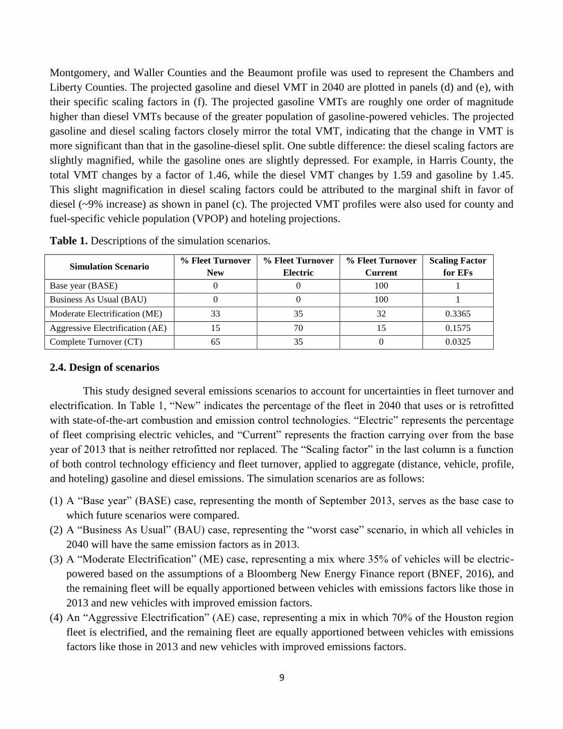
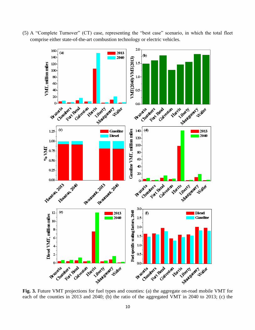
results are plotted in Fig. 3. Here, panel (a) represents the aggregate VMT (gasoline+diesel) for each of

the counties, and panel (b) represents the scaling factors, indicating an increase in VMT from 2013 to

2040 by 30%-80% over the eight-county area. Two surrogate gasoline-diesel split profiles, Houston and

Beaumont, were developed for the eight-county area. In panel (c), the gasoline-diesel split for VMT was

93%-7% for Houston and 82%-18% for Beaumont in 2013. The split changes marginally in favor of

diesel in 2040, 92%-8% for Houston and 81%-19% for Beaumont. The diesel fractions are higher over

suburban Beaumont while gasoline activities are significantly higher in the urban region (i.e., the city of

Houston). The Houston profile was used to represent the Brazoria, Fort Bend, Galveston, Harris,

9

Montgomery, and Waller Counties and the Beaumont profile was used to represent the Chambers and

Liberty Counties. The projected gasoline and diesel VMT in 2040 are plotted in panels (d) and (e), with

their specific scaling factors in (f). The projected gasoline VMTs are roughly one order of magnitude

higher than diesel VMTs because of the greater population of gasoline-powered vehicles. The projected

gasoline and diesel scaling factors closely mirror the total VMT, indicating that the change in VMT is

more significant than that in the gasoline-diesel split. One subtle difference: the diesel scaling factors are

slightly magnified, while the gasoline ones are slightly depressed. For example, in Harris County, the

total VMT changes by a factor of 1.46, while the diesel VMT changes by 1.59 and gasoline by 1.45.

This slight magnification in diesel scaling factors could be attributed to the marginal shift in favor of

diesel (~9% increase) as shown in panel (c). The projected VMT profiles were also used for county and

fuel-specific vehicle population (VPOP) and hoteling projections.

Table 1. Descriptions of the simulation scenarios.

Simulation Scenario % Fleet Turnover

New

% Fleet Turnover

Electric

% Fleet Turnover

Current

Scaling Factor

for EFs

Base year (BASE) 0 0 100 1

Business As Usual (BAU) 0 0 100 1

Moderate Electrification (ME) 33 35 32 0.3365

Aggressive Electrification (AE) 15 70 15 0.1575

Complete Turnover (CT) 65 35 0 0.0325

2.4. Design of scenarios

This study designed several emissions scenarios to account for uncertainties in fleet turnover and

electrification. In Table 1, “New” indicates the percentage of the fleet in 2040 that uses or is retrofitted

with state-of-the-art combustion and emission control technologies. “Electric” represents the percentage

of fleet comprising electric vehicles, and “Current” represents the fraction carrying over from the base

year of 2013 that is neither retrofitted nor replaced. The “Scaling factor” in the last column is a function

of both control technology efficiency and fleet turnover, applied to aggregate (distance, vehicle, profile,

and hoteling) gasoline and diesel emissions. The simulation scenarios are as follows:

(1) A “Base year” (BASE) case, representing the month of September 2013, serves as the base case to

which future scenarios were compared.

(2) A “Business As Usual” (BAU) case, representing the “worst case” scenario, in which all vehicles in

2040 will have the same emission factors as in 2013.

(3) A “Moderate Electrification” (ME) case, representing a mix where 35% of vehicles will be electric-

powered based on the assumptions of a Bloomberg New Energy Finance report (BNEF, 2016), and

the remaining fleet will be equally apportioned between vehicles with emissions factors like those in

2013 and new vehicles with improved emission factors.

(4) An “Aggressive Electrification” (AE) case, representing a mix in which 70% of the Houston region

fleet is electrified, and the remaining fleet are equally apportioned between vehicles with emissions

factors like those in 2013 and new vehicles with improved emissions factors.

10

(5) A “Complete Turnover” (CT) case, representing the “best case” scenario, in which the total fleet

comprise either state-of-the-art combustion technology or electric vehicles.

Fig. 3. Future VMT projections for fuel types and counties: (a) the aggregate on-road mobile VMT for

each of the counties in 2013 and 2040; (b) the ratio of the aggregated VMT in 2040 to 2013; (c) the

11

gasoline-diesel split of VMT; (d) similar to panel (a) but for gasoline VMT; (e) similar to panel (a) but

for diesel VMT; (f) similar to panel (b) but for gasoline and diesel separately. These projections are

based on calculations performed by the Texas Transportation Institute (TTI) for the Texas Commission

on Environmental Quality (TCEQ, 2015).

For all future year scenarios, mobile activity data (e.g., VMT, VPOP, and Hoteling) were increased to

the 2040 level, and projections of coal and natural gas EGUs were also applied.

2.5. Scaling factors for mobile emission factors

The effective emission factor calculation as described in the U.S. EPA’s National Mobile

Inventory Model (NMIM) is as follows:

𝐸𝐹𝑖(2040) = 𝐸𝐹𝑖(2013)[𝑓𝑟𝑒𝑝𝑙𝑎𝑐𝑒𝑑(1 − 𝑓𝑐𝑜𝑛𝑡𝑟𝑜𝑙) + 1 − 𝑓𝑟𝑒𝑝𝑙𝑎𝑐𝑒𝑑] (3)

where 𝐸𝐹𝑖(2040) and 𝐸𝐹𝑖(2013) are the emission factors for 2040 and 2013, respectively, 𝑓𝑟𝑒𝑝𝑙𝑎𝑐𝑒𝑑

represents the cumulative fraction of the fleet that has been replaced by newer, lower emitting sources

between 2013 and 2040, and 𝑓𝑐𝑜𝑛𝑡𝑟𝑜𝑙 represents the fractional reduction of emissions brought about by

this fleet replacement. The value of 𝑓𝑐𝑜𝑛𝑡𝑟𝑜𝑙 was assumed to be 95% based on Roy et al. (2014). To

include the portion of electric vehicles, the original Equation (3) was modified as follows:

𝐸𝐹𝑖(2040) = 𝐸𝐹𝑖(2013)[𝑓𝑁𝑒𝑤(1 − 𝑓𝑐𝑜𝑛𝑡𝑟𝑜𝑙) + 𝑓𝐸𝑙𝑒𝑐𝑡𝑟𝑖𝑐 × 0 + 𝑓𝐶𝑢𝑟𝑟𝑒𝑛𝑡] (4)

where 𝑓𝑁𝑒𝑤, 𝑓𝐸𝑙𝑒𝑐𝑡𝑟𝑖𝑐, and 𝑓𝐶𝑢𝑟𝑟𝑒𝑛𝑡 are the percentage fleet turnover values in Table 1. The scaling factor

values listed in Table 1 were obtained using equation (4). For instance, the scaling factor in the ME case

was:0.33 × (1 − 0.95) + 0.35 × 0 + 0.32 = 0.3365. It should be noted here we assumed zero

emissions from electric vehicles for easier demonstration. Electric vehicles produce no tailpipe exhaust

emissions. However, non-exhaust emissions (e.g., particulate matter emissions from brake and tire wear)

would not be significantly reduced and require technology improvement from those emission modes

(Soret et al., 2014).

2.6. Electricity demand and projections of EGUs

The added electricity required to power the motor vehicle fleet could potentially result in

increased emissions from Electricity Generating Units (EGUs). However, projections by the Electricity

Reliability Council of Texas (ERCOT, Borkar, et al., 2016) have indicated that the projected electricity

generation will be in western Texas, resulting in no new emissions in the eight-county area.

Additionally, ERCOT projections indicate a significant retirement of fossil-fired capacity for

southeastern Texas. Despite adding future capacity in the Houston region in our simulations, we needed

to account for capacity downsizing in order to represent a more realistic scenario in 2040. Assuming a

linear decline trend starting from 2013, we estimated factors of 0.89 and 0.99 (11% and 1% reductions)

and applied them to future EGUs powered by coal and natural gas, respectively.

Even though ERCOT projections indicate no new emissions in the Houston area, it is still

necessary to calculate the incremental electricity demand due to the vehicle electrification. Here, the

12

calculation was performed for the Aggressive Electrification scenario, which represented the highest

electricity consumption for electric vehicles and hence provided bounding estimates. The VMT data

from Fig. 3 were fractionated into New, Electric, and Current types. Each vehicle type was multiplied

using its specific energy consumption value per unit mile. Projections for electricity consumption (Wh

mile-1) for cars were taken from the Argonne National Laboratory (ANL)’s Autonomie model output.

For this, the Autonomie data on vehicle types had to be mapped to its MOVES counterpart. For

example, the energy consumption for a MOVES passenger car was assumed to be half that of

Autonomie compact and midsize combined. The mapping is detailed in Table S1. Electricity data for

trucks were adopted from the ANL’s AFLEET model (Burnham, 2017). The energy consumption values

(in Table S2 and S3) for each vehicle type, per unit mile, were multiplied with their specific VMT

values and summed up across all vehicle types to get a total electricity requirement. Additional details

for this calculation are listed in Section S2 of the Supplemental Information. The calculations for

additional electricity requirement indicated projected electrification load to be negligible (< 1%) of the

existing power plant generation. The reasons behind the low fraction could be the fact that Autonomie

projections account for improved technology and efficiency in 2040 representing lower energy

consumption. This coincides with the BNEF calculations that even as EVs represent 53% of global new

car sales, they only take up a small faction (~5%) of global power generation in 2040 (BNEF, 2017).

Hence, the incremental electricity demand was not considered in our simulations.

2.7. The health impact model

To evaluate the impact of these various scenarios on health and economic costs in the year 2040,

we used the U.S. EPA Environmental Benefits Mapping and Analysis Program (BenMAP) Community

Edition version 1.3 (U.S. EPA, 2017b). The air quality inputs of the model include a baseline scenario

(without control) and a control scenario (with an emission control policy implemented). In this study,

the base year case (2013) is the baseline scenario and the future year cases are different control

scenarios. The health impact calculations in BenMAP are based on concentration-response (C-R)

functions, typically representing a decrease in adverse health effects with a concentration of air

pollutants (Fann et al., 2012). One group of widely used C-R functions are in the log-linear format:

∆𝑦 = (1 − 𝑒−𝛽∙∆𝑥) × 𝑦0 × 𝑃𝑜𝑝 (5)

where ∆𝑦 represents the change in the incidence of adverse health effects, 𝛽 the concentration-response

coefficient, ∆𝑥 change in air quality (e.g., O3 concentrations), 𝑦0 the baseline incidence rates, and 𝑃𝑜𝑝

the affected population. The relationship between changes in air pollutant concentrations and incidence

of health outcome (i.e., 𝛽) are usually assessed in epidemiological studies. Additionally, the BenMAP

model calculates the economic cost of avoided premature mortality using a “value of statistical life”

(VSL) approach, which is the aggregate monetary value that a large group of people would be willing to

pay to slightly reduce the risk of premature death in the population (U.S. EPA, 2017b). The economic

costs for morbidities were estimated using the cost of illness, which includes direct medical costs and

lost earnings associated with illness.

13

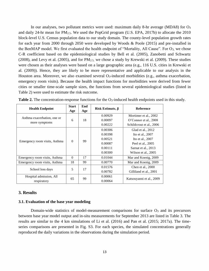
In our analyses, two pollutant metrics were used: maximum daily 8-hr average (MDA8) for O3

and daily 24-hr mean for PM2.5. We used the PopGrid program (U.S. EPA, 2017b) to allocate the 2010

block-level U.S. Census population data to our study domain. The county-level population growth rates

for each year from 2000 through 2050 were developed by Woods & Poole (2015) and pre-installed in

the BenMAP model. We first evaluated the health endpoint of “Mortality, All Cause”. For O3, we chose

C-R coefficient based on the epidemiological studies by Bell et al. (2005), Zanobetti and Schwartz

(2008), and Levy et al. (2005), and for PM2.5, we chose a study by Krewski et al. (2009). These studies

were chosen as their analyses were based on a large geographic area (e.g., 116 U.S. cities in Krewski et

al. (2009)). Hence, they are likely to be more representative and applicable to our analysis in the

Houston area. Moreover, we also examined several O3-induced morbidities (e.g., asthma exacerbation,

emergency room visits). Because the health impact functions for morbidities were derived from fewer

cities or smaller time-scale sample sizes, the functions from several epidemiological studies (listed in

Table 2) were used to estimate the risk outcome.

Table 2. The concentration-response functions for the O3-induced health endpoints used in this study.

Health Endpoint Start

Age

End

Age Risk Estimate, β Reference

Asthma exacerbation, one or

more symptoms 6 18

0.00929

0.00097

0.00222

Mortimer et al., 2002

O’Connor et al., 2008

Schildcrout et al., 2006

Emergency room visits, Asthma 0 99

0.00306

0.00398

0.00521

0.00087

0.00111

0.00300

Glad et al., 2012

Ito et al., 2007

Ito et al., 2007

Peel et al., 2005

Sarnat et al., 2013

Wilson et al., 2005

Emergency room visits, Asthma 0 17 0.01044 Mar and Koenig, 2009

Emergency room visits, Asthma 18 99 0.00770 Mar and Koenig, 2009

School loss days 5 17 0.01576

0.00782

Chen et al., 2000

Gilliland et al., 2001

Hospital admission, All

respiratory 65 99

0.00061

0.00064 Katsouyanni et al., 2009

3. Results

3.1. Evaluation of the base year modeling

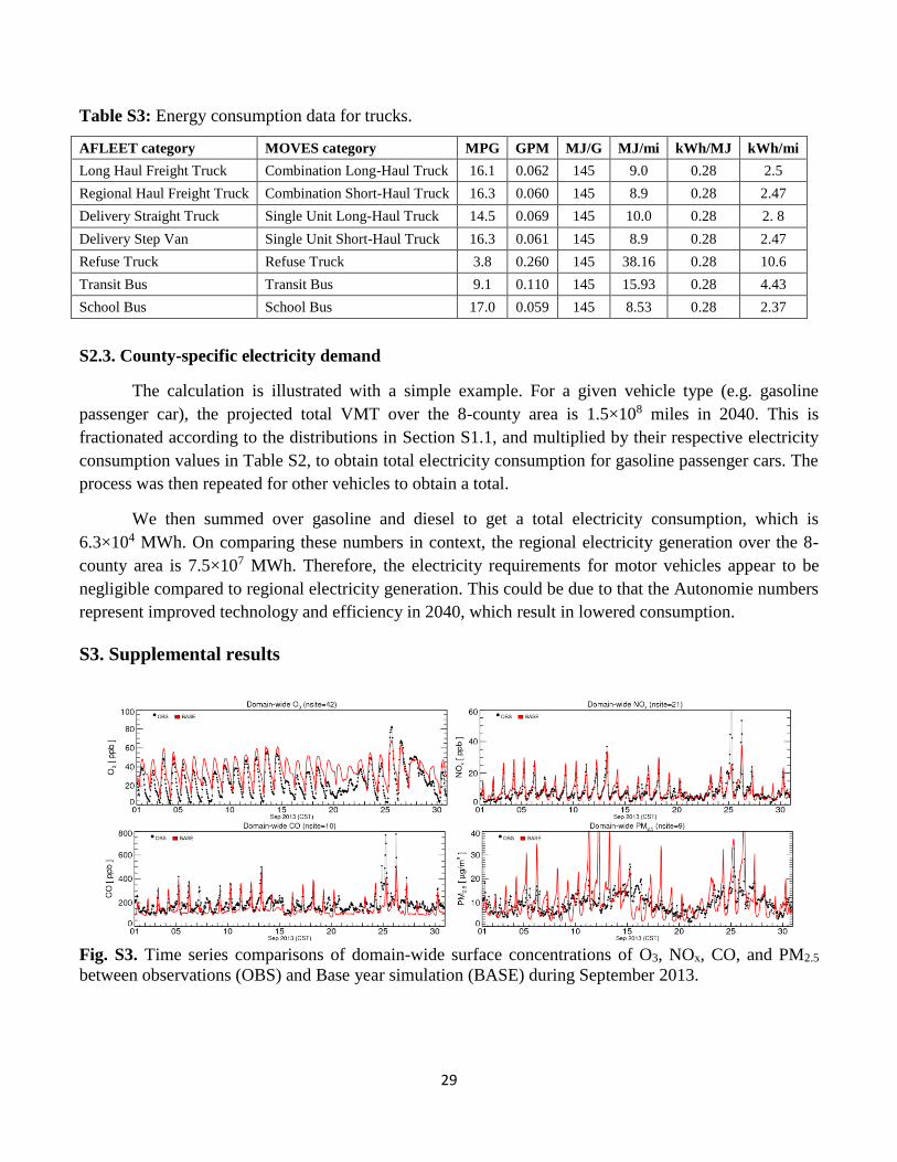
Domain-wide statistics of model-measurement comparisons for surface O3 and its precursors

between base year model output and in-situ measurements for September 2013 are listed in Table 3. The

results are similar to the 4 km simulations of Li et al. (2016) and Pan et al. (2015; 2017a). The time-

series comparisons are presented in Fig. S3. For each species, the simulated concentrations generally

reproduced the daily variations in the observations during the simulation period.

14

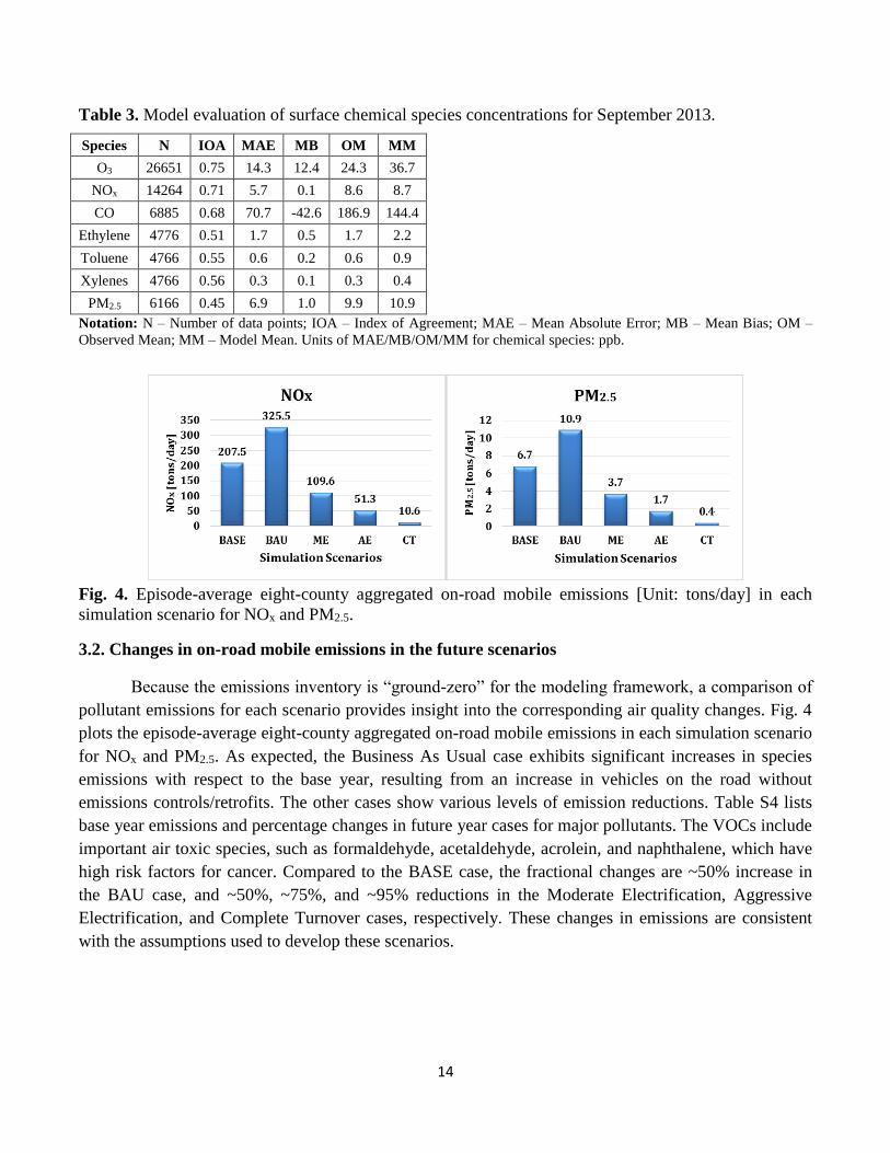
Table 3. Model evaluation of surface chemical species concentrations for September 2013.

Species N IOA MAE MB OM MM

O3 26651 0.75 14.3 12.4 24.3 36.7

NOx 14264 0.71 5.7 0.1 8.6 8.7

CO 6885 0.68 70.7 -42.6 186.9 144.4

Ethylene 4776 0.51 1.7 0.5 1.7 2.2

Toluene 4766 0.55 0.6 0.2 0.6 0.9

Xylenes 4766 0.56 0.3 0.1 0.3 0.4

PM2.5 6166 0.45 6.9 1.0 9.9 10.9

Notation: N – Number of data points; IOA – Index of Agreement; MAE – Mean Absolute Error; MB – Mean Bias; OM –

Observed Mean; MM – Model Mean. Units of MAE/MB/OM/MM for chemical species: ppb.

Fig. 4. Episode-average eight-county aggregated on-road mobile emissions [Unit: tons/day] in each

simulation scenario for NOx and PM2.5.

3.2. Changes in on-road mobile emissions in the future scenarios

Because the emissions inventory is “ground-zero” for the modeling framework, a comparison of

pollutant emissions for each scenario provides insight into the corresponding air quality changes. Fig. 4

plots the episode-average eight-county aggregated on-road mobile emissions in each simulation scenario

for NOx and PM2.5. As expected, the Business As Usual case exhibits significant increases in species

emissions with respect to the base year, resulting from an increase in vehicles on the road without

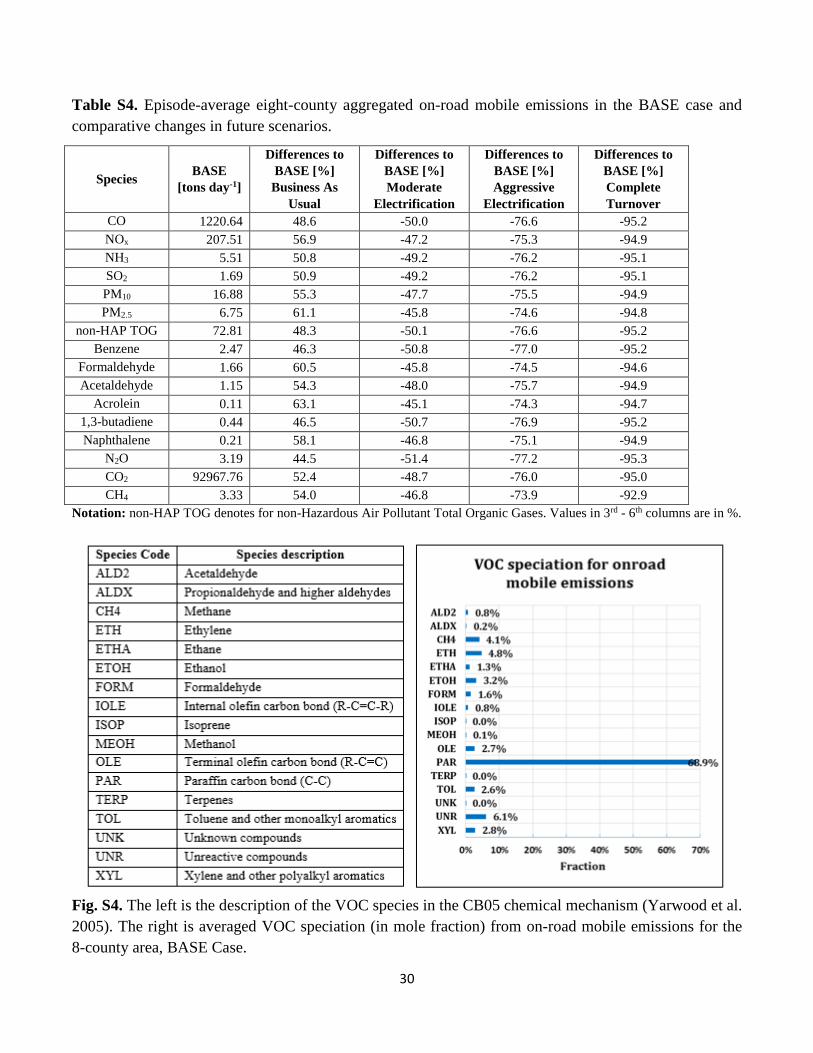
emissions controls/retrofits. The other cases show various levels of emission reductions. Table S4 lists

base year emissions and percentage changes in future year cases for major pollutants. The VOCs include

important air toxic species, such as formaldehyde, acetaldehyde, acrolein, and naphthalene, which have

high risk factors for cancer. Compared to the BASE case, the fractional changes are ~50% increase in

the BAU case, and ~50%, ~75%, and ~95% reductions in the Moderate Electrification, Aggressive

Electrification, and Complete Turnover cases, respectively. These changes in emissions are consistent

with the assumptions used to develop these scenarios.

15

Fig. 5. Spatial distributions of the surface concentrations of monthly average MDA8 O3, NOx, CO,

ethylene, toluene, xylenes, formaldehyde, isoprene, and terpenes during September 2013 for the BASE

case.

3.3. Spatial distributions of pollutants concentrations and projected future changes

3.3.1. Ozone and its precursors

Because O3 is a secondary pollutant, understanding the distributions of O3 precursors such as

NOx and dominant highly reactive VOC species is useful. Fig. S4 lists the descriptions of VOC species

in the CB05 chemical mechanism and the averaged VOC speciation from on-road mobile emissions in

the BASE case. The major highly reactive VOCs are ethylene (ETH, 4.8%), olefin (OLE+IOLE, 3.5%),

toluene (TOL, 2.6%), and xylenes (XYL, 2.8%). The paraffin (PAR, or alkanes) are only weakly

16

reactive with OH and ionic substances, even though they account for ~70% of the total on-road mobile

emissions. Fig. 5 plots the spatial distributions of base year surface O3 and its precursors (e.g., NOx, CO,

and several highly reactive VOC species). The MDA8 O3 hotspots are located northwest of the urban

center, where predominant wind originates from Galveston Bay and the Gulf of Mexico to the southeast

(Pan et al., 2017a). High NOx and CO concentrations are located over the urban area because of high

motor vehicle emissions. It is important to identify that NOx contours are steeper than CO due to the

shorter lifetime of NOx. While elevated ethylene concentrations are predicted over industrial regions,

toluene and xylenes concentrations are high over both industrial regions and urban road networks.

Formaldehyde hotspots coincide with non-point source oil and gas production regions, and isoprene and

terpenes concentrations are high over the northern part of the domain, resulting from significant

biogenic emissions generated by large forest cover.

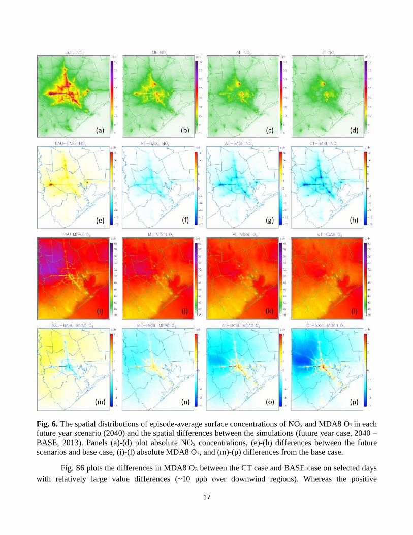
Fig. 6 plots the CMAQ-simulated NOx and MDA8 O3 concentrations for each scenario. The

results, shown in panels (a)-(d), plot a decrease in absolute NOx concentrations with increasing fleet

turnover, electrification, and control. For example, concentration hotspots are predicted over all highway

loops over Houston for the BAU case, and are predicted to significantly decrease in the CT case. In

other words, partial fleet electrification accompanied by complete fleet turnover result in lower NOx

emissions and thus, lower concentrations. Panels (i)-(l), which plot O3 concentrations, tell a different

story. The BAU case shows lowered MDA8 O3 concentrations over the highway loops and higher

concentrations elsewhere. Because highways have significant NOx emissions, they are NOx-saturated. In

such areas, O3 and NOx concentrations are inversely correlated, as previous studies (e.g., Choi et al.,

2012) illustrated. In addition, panel (i) illustrates increased O3 concentrations over regions northwest of

the loop, resulting from O3 formation in the outflow of NOx-saturated areas. The outflow regions are

NOx-limited and provide favorable conditions for O3 formation. With tighter controls, increased fleet

turnover, and decreasing NOx concentrations, O3 concentrations increase along the highway loop and

decrease over the outflow. Similar findings are corroborated in panels (m)-(p), which show the effects of

the O3 impacts vis-à-vis the 2013 base case. It is predicted that O3 concentrations resulting from

increased motor vehicle emissions decrease in the BAU case over the NOx-saturated areas by 1-3 ppb

while increasing 1-2 ppb over the outflow. Increasing controls, retrofits, electrification, and turnover

lead to lower NOx emissions and an increase in O3 concentrations by 1-3 ppb over the highways but

decrease over the entire outflow surrounding the highway loop, as well as the areas enclosed by the

loop. Notably, the CT case exhibit a decrease of 3-4 ppb over the northwestern outflow, the same region

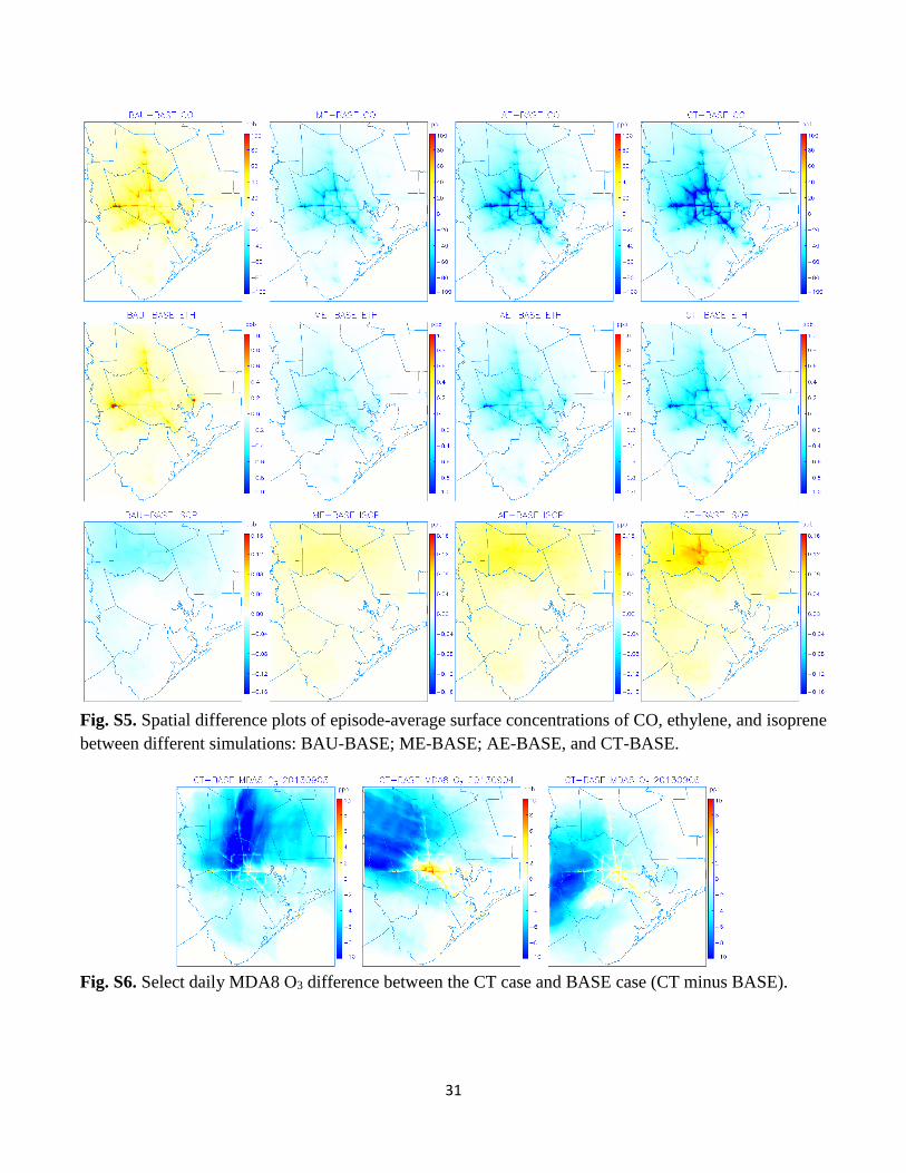
where a significant O3 increase is predicted in the BAU case. Fig. S5 displays the spatial differences for

CO, ethylene, and isoprene. The distributions of the change in CO and ethylene concentrations in future

year cases are similar to those in NOx concentrations. Whereas large positive changes in simulated

isoprene concentrations exist for the control cases over the northern domain, the decrease in isoprene

concentrations in the BAU case could be attributed to more indirect reactions with the enhanced NOx

emissions and concentrations (Diao et al., 2016). In high-NOx conditions, NOx serves as a sink for

isoprene. Isoprene reaction with hydroxyl radical (OH) in the presence of nitrogen oxide (NO) forms

isoprene nitrate or converts NO to NO2, which can undergo photolysis to form O3.

17

Fig. 6. The spatial distributions of episode-average surface concentrations of NOx and MDA8 O3 in each

future year scenario (2040) and the spatial differences between the simulations (future year case, 2040 –

BASE, 2013). Panels (a)-(d) plot absolute NOx concentrations, (e)-(h) differences between the future

scenarios and base case, (i)-(l) absolute MDA8 O3, and (m)-(p) differences from the base case.

Fig. S6 plots the differences in MDA8 O3 between the CT case and BASE case on selected days

with relatively large value differences (~10 ppb over downwind regions). Whereas the positive

18

difference areas are always located over the NOx-saturated urban roadways, the large negative areas

vary spatially because of day-to-day changes in wind direction, suggesting daily negative differences

(~10 ppb) could be much larger than episode-average MDA8 O3 reductions (3-4 ppb, in the last panel of

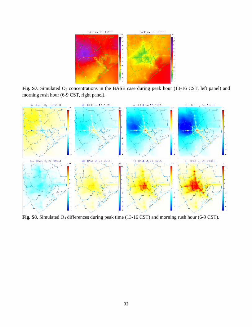
Fig. 6). Fig. S7 depicts the simulated base year O3 during the peak time (13-16 CST) and morning rush

hour (6-9 CST), and Fig. S8, the difference plots, illustrate the corresponding changes in future year

scenarios. The spatial distribution patterns of the BASE and difference O3 during the peak time are

similar to those of the MDA8 O3, but with higher magnitudes. During the morning rush hour, however,

the average O3 concentrations increase by ~10 ppb in the CT case, which results from NOx reductions

and less titration (last panel of Fig. S8). The morning O3 increase due to NOx reduction is also reported

by the study of vehicle electrification over the Yangtze River Delta region in China by Ke et al. (2017).

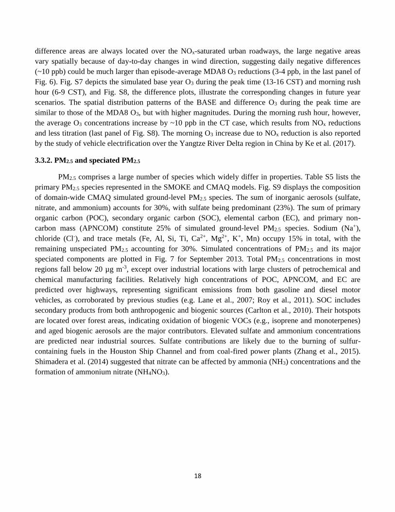
3.3.2. PM2.5 and speciated PM2.5

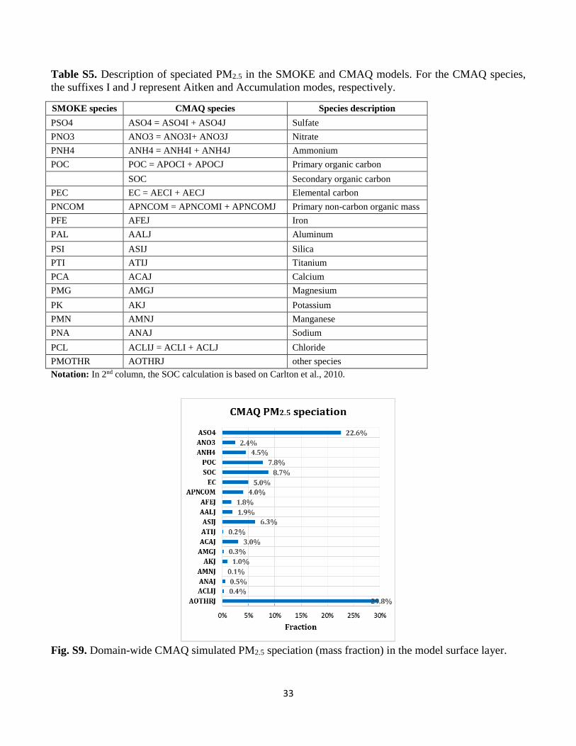
PM2.5 comprises a large number of species which widely differ in properties. Table S5 lists the

primary PM2.5 species represented in the SMOKE and CMAQ models. Fig. S9 displays the composition

of domain-wide CMAQ simulated ground-level PM2.5 species. The sum of inorganic aerosols (sulfate,

nitrate, and ammonium) accounts for 30%, with sulfate being predominant (23%). The sum of primary

organic carbon (POC), secondary organic carbon (SOC), elemental carbon (EC), and primary non-

carbon mass (APNCOM) constitute 25% of simulated ground-level PM2.5 species. Sodium (Na+),

chloride (Cl-), and trace metals (Fe, Al, Si, Ti, Ca2+, Mg2+, K+, Mn) occupy 15% in total, with the

remaining unspeciated PM2.5 accounting for 30%. Simulated concentrations of PM2.5 and its major

speciated components are plotted in Fig. 7 for September 2013. Total PM2.5 concentrations in most

regions fall below 20 µg m-3, except over industrial locations with large clusters of petrochemical and

chemical manufacturing facilities. Relatively high concentrations of POC, APNCOM, and EC are

predicted over highways, representing significant emissions from both gasoline and diesel motor

vehicles, as corroborated by previous studies (e.g. Lane et al., 2007; Roy et al., 2011). SOC includes

secondary products from both anthropogenic and biogenic sources (Carlton et al., 2010). Their hotspots

are located over forest areas, indicating oxidation of biogenic VOCs (e.g., isoprene and monoterpenes)

and aged biogenic aerosols are the major contributors. Elevated sulfate and ammonium concentrations

are predicted near industrial sources. Sulfate contributions are likely due to the burning of sulfur-

containing fuels in the Houston Ship Channel and from coal-fired power plants (Zhang et al., 2015).

Shimadera et al. (2014) suggested that nitrate can be affected by ammonia (NH3) concentrations and the

formation of ammonium nitrate (NH4NO3).

19

Fig. 7. Spatial distributions of surface concentrations of monthly average PM2.5 and major speciated

PM2.5 during September 2013 in the BASE case. (Acronyms: POC - primary organic carbon; APNCOM

- primary non-carbon mass; EC - elemental carbon; SOC - secondary organic carbon; AOTHRJ - other

unspeciated species).

20

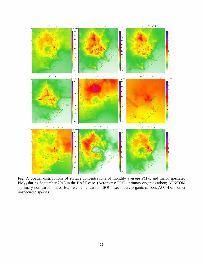
Fig. 8. The spatial difference of surface concentrations of monthly average total PM2.5, EC, POC, and

sulfate between different simulations: BAU-BASE; ME-BASE; AE-BASE, and CT-BASE.

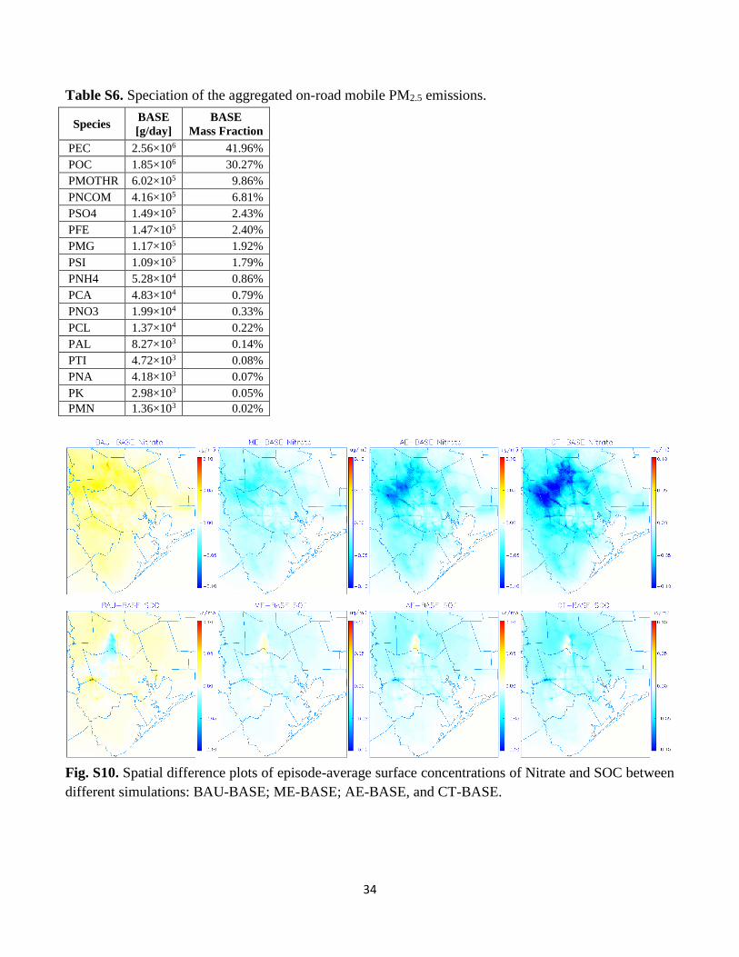
Because of the changes in mobile PM2.5 emissions in the future year cases, understanding the

major species that make up mobile emissions is useful and important. The SPECIATE databases (U.S.

EPA, 2017a) have reported that elemental carbon (EC) and organic carbon (OC) have high weight

fractions for PM2.5 speciation in transportation sources, such as Heavy Duty Diesel Vehicles (HDDV)

21

exhaust (EC: 77%; OC: 17.5%), Light Duty Diesel Vehicles (LDDV) exhaust (EC: 51.4%; OC: 35.5%),

and on-road gasoline exhaust (EC: 19%; OC: 55%). Here, we calculated the mass fraction of each PM2.5

component in the aggregated on-road mobile emissions in Table S6. Species with higher fractions will

undergo a relatively substantial change in the future year cases, as opposed to those with lower fractions.

Similarly, the two biggest components of PM2.5 are elemental carbon (42%) and primary organic carbon

(30%). Thus, the changes in total PM2.5 concentrations are mainly associated with changes in

carbonaceous species. Fig. 8 plots the differences between the projected scenarios and the base 2013

case. Panels (a)-(d) represent total PM2.5 concentrations. The BAU case results in an increase in PM2.5

concentrations of 1-2 μg m-3, while the control scenarios show decreases in PM2.5 concentrations ranging

from 0.5-2 μg m-3. The most dramatic changes occur on highways because of reductions in motor

vehicle emissions, corroborated in the plots for EC (panels (e)-(h)) and POC (panels (i)-(l)). The

changes in sulfate also mirror those of EC and POC, but one additional important point is the reduction

in sulfate hotspots over regions with EGU emissions, due to the reduction in coal capacity over these

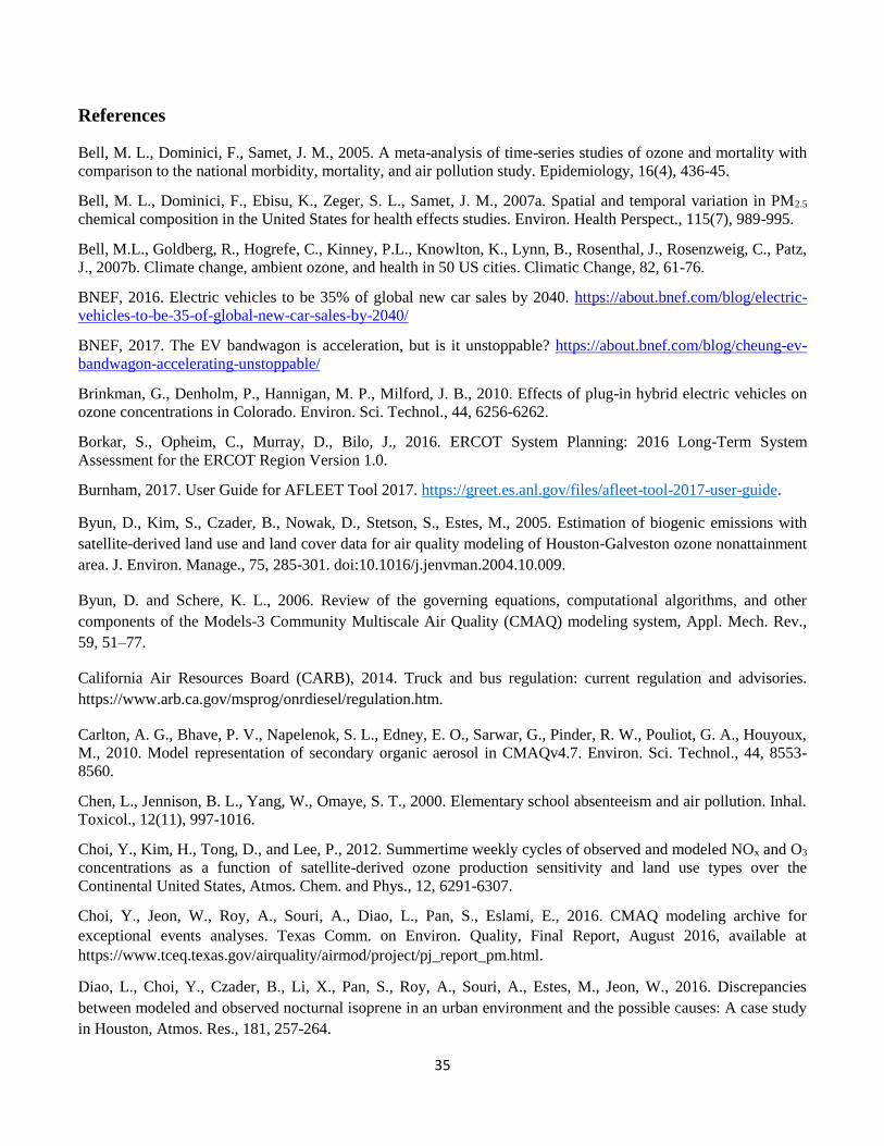
areas. The changes in PM2.5 concentrations could also be attributable to other chemical reactions

associated with gas-to-particle conversion (e.g., HNO3(g)→nitrate). In all the control scenarios, the

reduced NOx, a precursor for HNO3, contributed to the decreased nitrate concentrations over the

downwind northwest (Fig. S10). Moreover, the decreased VOCs emissions in the urban area also lead to

reduction in the concentrations of secondary organic carbon.

3.4. Evaluation of the changes in health endpoints and benefits

The health impact calculations in BenMAP are based on concentration-response (C-R) functions,

which represent a decrease in health incidence with air pollutant concentrations. Based on these

calculations, the BAU case would likely result in an increased number of premature deaths with respect

to 2013. All of the control scenarios, however, would result in prevented mortality, as shown in Table 4.

For PM2.5, the table shows about 121 more premature deaths in the BAU case over greater Houston, and

109, 177, and 229 prevented premature deaths in the ME, AE, and CT cases, respectively. These

findings coincide with trends in PM2.5 concentration, as depicted in panels (a)-(d) in Fig. 8. The findings

also roughly correspond to a 61% increase in PM2.5 emissions in the BAU case, and 46%, 75%, and 95%

reductions in the ME, AE, and CT cases listed in Table S4.

Interpreting the O3 results, however, is more complicated because the trends of O3 change vary

spatially (panels (m)-(p) of Fig. 6). For instance, in the BAU case, BenMAP predicts an increase in

adverse health effects over downwind areas because of O3 increases, while predicting a decrease of

damage in the urban and major highways. The net number of premature deaths is negligible at -0.04, and

indicates that the downwind negative impact is barely larger than the positive impacts in the urban area.

In contrast, for the other scenarios with emissions reductions (i.e., the ME, AE, and CT cases), the gains

in health endpoints in downwind areas are all greater than the losses over the urban highways, resulting

in about 5, 11, and 17 prevented premature deaths, respectively. We may expect more health benefits if

the simulation domain were to cover more downwind areas. It should be noted that even in the case of

an increase in O3 concentrations over the urban highways, reductions in air toxics emissions would

occur, which would lead to more health benefits not studied here because the health impact functions for

22

these air toxics are not available in the current BenMAP model. The economic cost (benefit) values

generally coincide with premature mortality results.

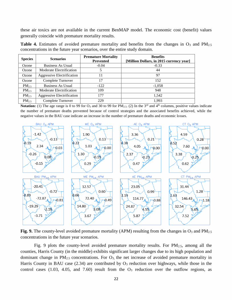
Table 4. Estimates of avoided premature mortality and benefits from the changes in O3 and PM2.5

concentrations in the future year scenarios, over the entire study domain.

Species Scenarios Premature Mortality

Prevented

Benefits

[Million Dollars, in 2015 currency year]

Ozone Business As Usual -0.04 -0.33

Ozone Moderate Electrification 5 44

Ozone Aggressive Electrification 11 97

Ozone Complete Turnover 17 152

PM2.5 Business As Usual -122 -1,058

PM2.5 Moderate Electrification 109 948

PM2.5 Aggressive Electrification 177 1,542

PM2.5 Complete Turnover 229 1,993

Notation: (1) The age range is 0 to 99 for O3 and 30 to 99 for PM2.5. (2) In the 3rd and 4th columns, positive values indicate

the number of premature deaths prevented because of control strategies and the associated benefits achieved, while the

negative values in the BAU case indicate an increase in the number of premature deaths and economic losses.

Fig. 9. The county-level avoided premature mortality (APM) resulting from the changes in O3 and PM2.5

concentrations in the future year scenarios.

Fig. 9 plots the county-level avoided premature mortality results. For PM2.5, among all the

counties, Harris County (in the middle) exhibits significant larger changes due to its high population and

dominant change in PM2.5 concentrations. For O3, the net increase of avoided premature mortality in

Harris County in BAU case (2.34) are contributed by O3 reduction over highways, while those in the

control cases (1.03, 4.05, and 7.60) result from the O3 reduction over the outflow regions, as

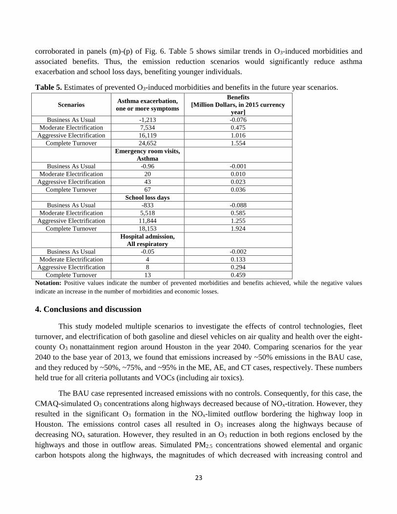
23

corroborated in panels (m)-(p) of Fig. 6. Table 5 shows similar trends in O3-induced morbidities and

associated benefits. Thus, the emission reduction scenarios would significantly reduce asthma

exacerbation and school loss days, benefiting younger individuals.

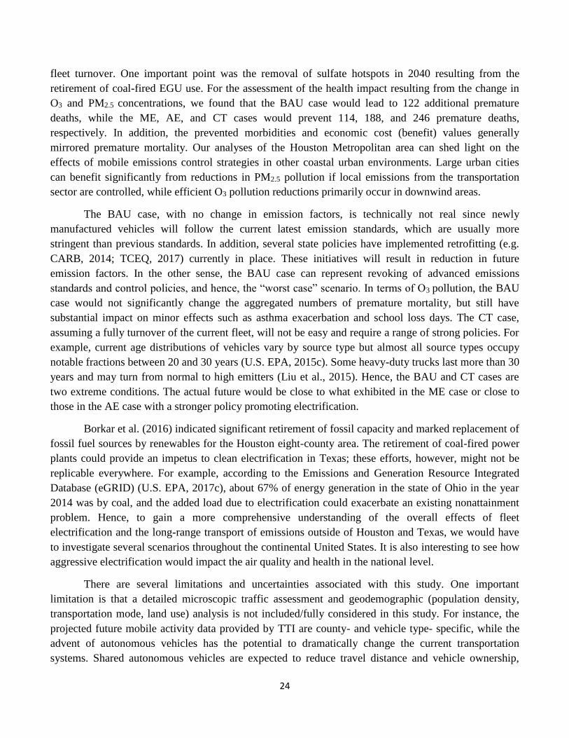
Table 5. Estimates of prevented O3-induced morbidities and benefits in the future year scenarios.

Scenarios Asthma exacerbation,

one or more symptoms

Benefits

[Million Dollars, in 2015 currency

year]

Business As Usual -1,213 -0.076

Moderate Electrification 7,534 0.475

Aggressive Electrification 16,119 1.016

Complete Turnover 24,652 1.554

Emergency room visits,

Asthma

Business As Usual -0.96 -0.001

Moderate Electrification 20 0.010

Aggressive Electrification 43 0.023

Complete Turnover 67 0.036

School loss days

Business As Usual -833 -0.088

Moderate Electrification 5,518 0.585

Aggressive Electrification 11,844 1.255

Complete Turnover 18,153 1.924

Hospital admission,

All respiratory

Business As Usual -0.05 -0.002

Moderate Electrification 4 0.133

Aggressive Electrification 8 0.294

Complete Turnover 13 0.459

Notation: Positive values indicate the number of prevented morbidities and benefits achieved, while the negative values

indicate an increase in the number of morbidities and economic losses.

4. Conclusions and discussion

This study modeled multiple scenarios to investigate the effects of control technologies, fleet

turnover, and electrification of both gasoline and diesel vehicles on air quality and health over the eight-

county O3 nonattainment region around Houston in the year 2040. Comparing scenarios for the year

2040 to the base year of 2013, we found that emissions increased by ~50% emissions in the BAU case,

and they reduced by ~50%, ~75%, and ~95% in the ME, AE, and CT cases, respectively. These numbers

held true for all criteria pollutants and VOCs (including air toxics).

The BAU case represented increased emissions with no controls. Consequently, for this case, the

CMAQ-simulated O3 concentrations along highways decreased because of NOx-titration. However, they

resulted in the significant O3 formation in the NOx-limited outflow bordering the highway loop in

Houston. The emissions control cases all resulted in O3 increases along the highways because of

decreasing NOx saturation. However, they resulted in an O3 reduction in both regions enclosed by the

highways and those in outflow areas. Simulated PM2.5 concentrations showed elemental and organic

carbon hotspots along the highways, the magnitudes of which decreased with increasing control and

24

fleet turnover. One important point was the removal of sulfate hotspots in 2040 resulting from the

retirement of coal-fired EGU use. For the assessment of the health impact resulting from the change in

O3 and PM2.5 concentrations, we found that the BAU case would lead to 122 additional premature

deaths, while the ME, AE, and CT cases would prevent 114, 188, and 246 premature deaths,

respectively. In addition, the prevented morbidities and economic cost (benefit) values generally

mirrored premature mortality. Our analyses of the Houston Metropolitan area can shed light on the

effects of mobile emissions control strategies in other coastal urban environments. Large urban cities

can benefit significantly from reductions in PM2.5 pollution if local emissions from the transportation

sector are controlled, while efficient O3 pollution reductions primarily occur in downwind areas.

The BAU case, with no change in emission factors, is technically not real since newly

manufactured vehicles will follow the current latest emission standards, which are usually more

stringent than previous standards. In addition, several state policies have implemented retrofitting (e.g.

CARB, 2014; TCEQ, 2017) currently in place. These initiatives will result in reduction in future

emission factors. In the other sense, the BAU case can represent revoking of advanced emissions

standards and control policies, and hence, the “worst case” scenario. In terms of O3 pollution, the BAU

case would not significantly change the aggregated numbers of premature mortality, but still have

substantial impact on minor effects such as asthma exacerbation and school loss days. The CT case,

assuming a fully turnover of the current fleet, will not be easy and require a range of strong policies. For

example, current age distributions of vehicles vary by source type but almost all source types occupy

notable fractions between 20 and 30 years (U.S. EPA, 2015c). Some heavy-duty trucks last more than 30

years and may turn from normal to high emitters (Liu et al., 2015). Hence, the BAU and CT cases are

two extreme conditions. The actual future would be close to what exhibited in the ME case or close to

those in the AE case with a stronger policy promoting electrification.

Borkar et al. (2016) indicated significant retirement of fossil capacity and marked replacement of

fossil fuel sources by renewables for the Houston eight-county area. The retirement of coal-fired power

plants could provide an impetus to clean electrification in Texas; these efforts, however, might not be

replicable everywhere. For example, according to the Emissions and Generation Resource Integrated

Database (eGRID) (U.S. EPA, 2017c), about 67% of energy generation in the state of Ohio in the year

2014 was by coal, and the added load due to electrification could exacerbate an existing nonattainment

problem. Hence, to gain a more comprehensive understanding of the overall effects of fleet

electrification and the long-range transport of emissions outside of Houston and Texas, we would have

to investigate several scenarios throughout the continental United States. It is also interesting to see how

aggressive electrification would impact the air quality and health in the national level.

There are several limitations and uncertainties associated with this study. One important

limitation is that a detailed microscopic traffic assessment and geodemographic (population density,

transportation mode, land use) analysis is not included/fully considered in this study. For instance, the

projected future mobile activity data provided by TTI are county- and vehicle type- specific, while the

advent of autonomous vehicles has the potential to dramatically change the current transportation

systems. Shared autonomous vehicles are expected to reduce travel distance and vehicle ownership,

25

impacting on land use (e.g., parking infrastructure) and travel patterns (Shaheen and Cohen, 2013;

Fagnant and Kockelman, 2014). Hence, the diurnal and spatial patterns of mobile emissions may also

change. In addition, the population growth rates in the health impact model are at county-level, while the

distribution of population could possibly change within each county. In this study, we made projections

for on-road mobile and EGUs sectors, the emissions for other sectors were fixed to present levels. The

meteorological conditions and chemical boundaries were also kept unchanged. These would affect the

future total air quality levels (Bell et al., 2007a; 2007b). Another uncertainty is that we applied fixed

fractional rates of fleet turnover and control factor. The actual vehicle fleet composition may vary in the

future and largely depend on policy, pricing, and technology. But the future emissions should fall

between our four scenarios here. Also if technologies are not ready in 2040 to reduce non-exhaust

emissions (e.g., PM2.5 emissions from brake and tire wear) from electric fleet, the corresponding change

in PM2.5 concentrations and health outcomes would likely be smaller than the numbers reported in this

study.

In the health impact analysis, the C-R relationships are derived from long-term air quality

measurements and health records data, while only one month simulations were used here because the

1×1 km simulations were too computational expensive. Hence the health impact results may be over- or

under- estimated if seasonal variation of air pollutants concentrations are considered. In addition, the

uncertainties in emissions may impact the air quality and health outcomes. For instance, McDonald et al.

(2018) reported the over-prediction of NOx mobile emissions in the National Emission Inventory. In our

study, if the NOx mobile emissions are over-predicted in the base case, then the change in NOx

emissions or concentrations between the base and future year cases would be smaller than the numbers

reported in this study, resulting potential less change in O3 concentrations and subsequent over-

prediction of the health outcomes. While also as suggested by McDonald et al. (2018), reduction in

mobile source NOx emissions could help reducing the number of high O3 days in the Eastern U.S. and

meeting more stringent O3 standards in the future. In our cases, the fleet electrification could possibly

lead to less emissions accumulation during the meteorological conditions favoring O3 production (e.g.,

land-bay/sea breeze recirculation, early morning low wind speeds), and potential less events of O3

exceedance. Overall, this study provides proof-of-concept of how the combined effects of a greening

grid, emissions control, and fleet electrification can improve air quality and human health.

Acknowledgements

The authors acknowledge the support from the U.S. Department of Transportation (DOT) Center

for Transportation, Environment, and Community Health (CTECH). The authors thank the contributions

from Anirban Roy, Yunsoo Choi, and Ebrahim Eslami (University of Houston), Stephanie Thomas and

Thomas Smith (Public Citizen), Xiangyu Jiang (University at Buffalo), Dennis Perkinson (Texas

Transportation Institute), and Warren Lasher (Electric Reliability Council of Texas).

26

Supplemental Information

S1. A simplified flow chart of the air quality modeling system

Fig. S1. A simplified flow chart of the air quality modeling system.

S2. Calculations of electricity demand

S2.1. Fleet turnover with new and electric vehicles

This calculation was performed for the Aggressive Electrification scenario, which represents the

highest electricity consumption for electric and hybrid vehicles and hence provides bounding estimates.

The VMT data were fractionated into New, Electric, and Current types.

For light-duty “New” vehicles, we assume new technologies will all be hybrid, since major

automobile manufacturers such as Volvo and Jaguar-Land Rover have already announced plans to build

only hybrid vehicles post-2020. The United States Department of Energy (U.S. DOE)’s Energy

Information Administration (EIA)’s Annual Energy Outlook of 2018 (AEO2018) provides the

categories of hybrid (HEV), plug-in hybrid (PHEV), and all-electric vehicles (BEV) differing in range.

According to the report, the proportion of electric vehicles with all-electric range (AER) 100, 200 and

300 in 2040 was projected to be 1:5:5 roughly, translating into overall fractions of 0.0636, 0.318 and

0.318 respectively (adding up to 0.7 that represents total “Electric” fraction). Similarly, the ratio of

standard to plug-in hybrids was projected by the AEO to be roughly 3:1, resulting in 0.116 of hybrid and

0.034 of plug-in hybrid (adding up to 0.15 that represents total “New” fraction). The Argonne National

Laboratory’s Autonomie data further indicate PHEVs will be of four types, namely PHEV10, PHEV20,

PHEV30 and PHEV40. In the absence of information, each of these assumed to have an equal share.

For heavy-duty diesel vehicles, in absence of adequate information on hybrid projections, we

assume all new vehicles to be electric vehicles, resulting in 85% of electric vehicles in 2040.

27

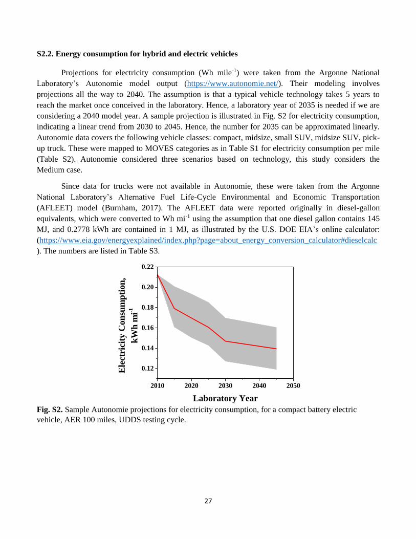
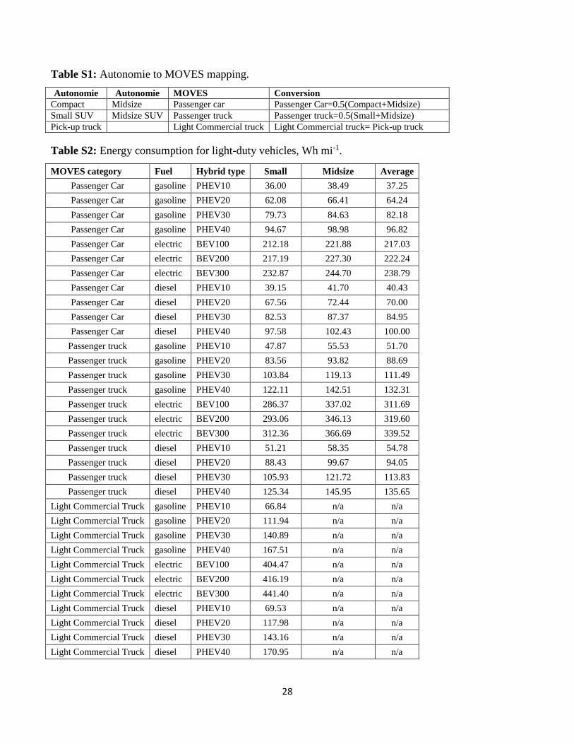
S2.2. Energy consumption for hybrid and electric vehicles

Projections for electricity consumption (Wh mile-1) were taken from the Argonne National

Laboratory’s Autonomie model output (https://www.autonomie.net/). Their modeling involves

projections all the way to 2040. The assumption is that a typical vehicle technology takes 5 years to

reach the market once conceived in the laboratory. Hence, a laboratory year of 2035 is needed if we are

considering a 2040 model year. A sample projection is illustrated in Fig. S2 for electricity consumption,

indicating a linear trend from 2030 to 2045. Hence, the number for 2035 can be approximated linearly.

Autonomie data covers the following vehicle classes: compact, midsize, small SUV, midsize SUV, pick-

up truck. These were mapped to MOVES categories as in Table S1 for electricity consumption per mile

(Table S2). Autonomie considered three scenarios based on technology, this study considers the

Medium case.

Since data for trucks were not available in Autonomie, these were taken from the Argonne

National Laboratory’s Alternative Fuel Life-Cycle Environmental and Economic Transportation

(AFLEET) model (Burnham, 2017). The AFLEET data were reported originally in diesel-gallon

equivalents, which were converted to Wh mi-1 using the assumption that one diesel gallon contains 145

MJ, and 0.2778 kWh are contained in 1 MJ, as illustrated by the U.S. DOE EIA’s online calculator:

(https://www.eia.gov/energyexplained/index.php?page=about_energy_conversion_calculator#dieselcalc

). The numbers are listed in Table S3.

2010 2020 2030 2040 2050

0.12

0.14

0.16

0.18

0.20

0.22

Ele

ctri

city

Con

sum

pti

on

,

kW

h m

i-1

Laboratory Year Fig. S2. Sample Autonomie projections for electricity consumption, for a compact battery electric

vehicle, AER 100 miles, UDDS testing cycle.

https://www.autonomie.net/

https://www.eia.gov/energyexplained/index.php?page=about_energy_conversion_calculator#dieselcalc

https://www.eia.gov/energyexplained/index.php?page=about_energy_conversion_calculator#dieselcalc

28

Table S1: Autonomie to MOVES mapping.

Autonomie Autonomie MOVES Conversion

Compact Midsize Passenger car Passenger Car=0.5(Compact+Midsize)

Small SUV Midsize SUV Passenger truck Passenger truck=0.5(Small+Midsize)

Pick-up truck Light Commercial truck Light Commercial truck= Pick-up truck

Table S2: Energy consumption for light-duty vehicles, Wh mi-1.

MOVES category Fuel Hybrid type Small Midsize Average

Passenger Car gasoline PHEV10 36.00 38.49 37.25




Passenger Car electric BEV100 212.18 221.88 217.03



Passenger Car diesel PHEV10 39.15 41.70 40.43




Passenger truck gasoline PHEV10 47.87 55.53 51.70




Passenger truck electric BEV100 286.37 337.02 311.69



Passenger truck diesel PHEV10 51.21 58.35 54.78




Light Commercial Truck gasoline PHEV10 66.84 n/a n/a




Light Commercial Truck electric BEV100 404.47 n/a n/a



Light Commercial Truck diesel PHEV10 69.53 n/a n/a




29

Table S3: Energy consumption data for trucks.

AFLEET category MOVES category MPG GPM MJ/G MJ/mi kWh/MJ kWh/mi

Long Haul Freight Truck Combination Long-Haul Truck 16.1 0.062 145 9.0 0.28 2.5

Regional Haul Freight Truck Combination Short-Haul Truck 16.3 0.060 145 8.9 0.28 2.47

Delivery Straight Truck Single Unit Long-Haul Truck 14.5 0.069 145 10.0 0.28 2. 8

Delivery Step Van Single Unit Short-Haul Truck 16.3 0.061 145 8.9 0.28 2.47

Refuse Truck Refuse Truck 3.8 0.260 145 38.16 0.28 10.6

Transit Bus Transit Bus 9.1 0.110 145 15.93 0.28 4.43

School Bus School Bus 17.0 0.059 145 8.53 0.28 2.37

S2.3. County-specific electricity demand

The calculation is illustrated with a simple example. For a given vehicle type (e.g. gasoline

passenger car), the projected total VMT over the 8-county area is 1.5×108 miles in 2040. This is

fractionated according to the distributions in Section S1.1, and multiplied by their respective electricity

consumption values in Table S2, to obtain total electricity consumption for gasoline passenger cars. The

process was then repeated for other vehicles to obtain a total.

We then summed over gasoline and diesel to get a total electricity consumption, which is

6.3×104 MWh. On comparing these numbers in context, the regional electricity generation over the 8-

county area is 7.5×107 MWh. Therefore, the electricity requirements for motor vehicles appear to be

negligible compared to regional electricity generation. This could be due to that the Autonomie numbers

represent improved technology and efficiency in 2040, which result in lowered consumption.

S3. Supplemental results

Fig. S3. Time series comparisons of domain-wide surface concentrations of O3, NOx, CO, and PM2.5

between observations (OBS) and Base year simulation (BASE) during September 2013.

30

Table S4. Episode-average eight-county aggregated on-road mobile emissions in the BASE case and

comparative changes in future scenarios.

Species BASE

[tons day-1]

Differences to

BASE [%]

Business As

Usual

Differences to

BASE [%]

Moderate

Electrification

Differences to

BASE [%]

Aggressive

Electrification

Differences to

BASE [%]

Complete

Turnover

CO 1220.64 48.6 -50.0 -76.6 -95.2

NOx 207.51 56.9 -47.2 -75.3 -94.9

NH3 5.51 50.8 -49.2 -76.2 -95.1

SO2 1.69 50.9 -49.2 -76.2 -95.1

PM10 16.88 55.3 -47.7 -75.5 -94.9

PM2.5 6.75 61.1 -45.8 -74.6 -94.8

non-HAP TOG 72.81 48.3 -50.1 -76.6 -95.2

Benzene 2.47 46.3 -50.8 -77.0 -95.2

Formaldehyde 1.66 60.5 -45.8 -74.5 -94.6

Acetaldehyde 1.15 54.3 -48.0 -75.7 -94.9

Acrolein 0.11 63.1 -45.1 -74.3 -94.7

1,3-butadiene 0.44 46.5 -50.7 -76.9 -95.2

Naphthalene 0.21 58.1 -46.8 -75.1 -94.9

N2O 3.19 44.5 -51.4 -77.2 -95.3

CO2 92967.76 52.4 -48.7 -76.0 -95.0

CH4 3.33 54.0 -46.8 -73.9 -92.9

Notation: non-HAP TOG denotes for non-Hazardous Air Pollutant Total Organic Gases. Values in 3rd - 6th columns are in %.

Fig. S4. The left is the description of the VOC species in the CB05 chemical mechanism (Yarwood et al.

2005). The right is averaged VOC speciation (in mole fraction) from on-road mobile emissions for the

8-county area, BASE Case.

31

Fig. S5. Spatial difference plots of episode-average surface concentrations of CO, ethylene, and isoprene

between different simulations: BAU-BASE; ME-BASE; AE-BASE, and CT-BASE.

Fig. S6. Select daily MDA8 O3 difference between the CT case and BASE case (CT minus BASE).

32

Fig. S7. Simulated O3 concentrations in the BASE case during peak hour (13-16 CST, left panel) and

morning rush hour (6-9 CST, right panel).

Fig. S8. Simulated O3 differences during peak time (13-16 CST) and morning rush hour (6-9 CST).

33

Table S5. Description of speciated PM2.5 in the SMOKE and CMAQ models. For the CMAQ species,

the suffixes I and J represent Aitken and Accumulation modes, respectively.

SMOKE species CMAQ species Species description

PSO4 ASO4 = ASO4I + ASO4J Sulfate

PNO3 ANO3 = ANO3I+ ANO3J Nitrate

PNH4 ANH4 = ANH4I + ANH4J Ammonium

POC POC = APOCI + APOCJ Primary organic carbon

SOC Secondary organic carbon

PEC EC = AECI + AECJ Elemental carbon

PNCOM APNCOM = APNCOMI + APNCOMJ Primary non-carbon organic mass

PFE AFEJ Iron

PAL AALJ Aluminum

PSI ASIJ Silica

PTI ATIJ Titanium

PCA ACAJ Calcium

PMG AMGJ Magnesium

PK AKJ Potassium

PMN AMNJ Manganese

PNA ANAJ Sodium

PCL ACLIJ = ACLI + ACLJ Chloride

PMOTHR AOTHRJ other species

Notation: In 2nd column, the SOC calculation is based on Carlton et al., 2010.

Fig. S9. Domain-wide CMAQ simulated PM2.5 speciation (mass fraction) in the model surface layer.

34

Table S6. Speciation of the aggregated on-road mobile PM2.5 emissions.

Species BASE

[g/day]

BASE

Mass Fraction

PEC 2.56×106 41.96%

POC 1.85×106 30.27%

PMOTHR 6.02×105 9.86%

PNCOM 4.16×105 6.81%

PSO4 1.49×105 2.43%

PFE 1.47×105 2.40%

PMG 1.17×105 1.92%

PSI 1.09×105 1.79%

PNH4 5.28×104 0.86%

PCA 4.83×104 0.79%

PNO3 1.99×104 0.33%

PCL 1.37×104 0.22%

PAL 8.27×103 0.14%

PTI 4.72×103 0.08%

PNA 4.18×103 0.07%

PK 2.98×103 0.05%

PMN 1.36×103 0.02%

Fig. S10. Spatial difference plots of episode-average surface concentrations of Nitrate and SOC between

different simulations: BAU-BASE; ME-BASE; AE-BASE, and CT-BASE.

35

References

Bell, M. L., Dominici, F., Samet, J. M., 2005. A meta-analysis of time-series studies of ozone and mortality with

comparison to the national morbidity, mortality, and air pollution study. Epidemiology, 16(4), 436-45.

Bell, M. L., Dominici, F., Ebisu, K., Zeger, S. L., Samet, J. M., 2007a. Spatial and temporal variation in PM2.5

chemical composition in the United States for health effects studies. Environ. Health Perspect., 115(7), 989-995.

Bell, M.L., Goldberg, R., Hogrefe, C., Kinney, P.L., Knowlton, K., Lynn, B., Rosenthal, J., Rosenzweig, C., Patz,

J., 2007b. Climate change, ambient ozone, and health in 50 US cities. Climatic Change, 82, 61-76.

BNEF, 2016. Electric vehicles to be 35% of global new car sales by 2040. https://about.bnef.com/blog/electric-

vehicles-to-be-35-of-global-new-car-sales-by-2040/

BNEF, 2017. The EV bandwagon is acceleration, but is it unstoppable? https://about.bnef.com/blog/cheung-ev-

bandwagon-accelerating-unstoppable/

Brinkman, G., Denholm, P., Hannigan, M. P., Milford, J. B., 2010. Effects of plug-in hybrid electric vehicles on

ozone concentrations in Colorado. Environ. Sci. Technol., 44, 6256-6262.

Borkar, S., Opheim, C., Murray, D., Bilo, J., 2016. ERCOT System Planning: 2016 Long-Term System

Assessment for the ERCOT Region Version 1.0.

Burnham, 2017. User Guide for AFLEET Tool 2017. https://greet.es.anl.gov/files/afleet-tool-2017-user-guide.

Byun, D., Kim, S., Czader, B., Nowak, D., Stetson, S., Estes, M., 2005. Estimation of biogenic emissions with

satellite-derived land use and land cover data for air quality modeling of Houston-Galveston ozone nonattainment

area. J. Environ. Manage., 75, 285-301. doi:10.1016/j.jenvman.2004.10.009.

Byun, D. and Schere, K. L., 2006. Review of the governing equations, computational algorithms, and other

components of the Models-3 Community Multiscale Air Quality (CMAQ) modeling system, Appl. Mech. Rev.,

59, 51–77.

California Air Resources Board (CARB), 2014. Truck and bus regulation: current regulation and advisories.

https://www.arb.ca.gov/msprog/onrdiesel/regulation.htm.

Carlton, A. G., Bhave, P. V., Napelenok, S. L., Edney, E. O., Sarwar, G., Pinder, R. W., Pouliot, G. A., Houyoux,

M., 2010. Model representation of secondary organic aerosol in CMAQv4.7. Environ. Sci. Technol., 44, 8553-

8560.

Chen, L., Jennison, B. L., Yang, W., Omaye, S. T., 2000. Elementary school absenteeism and air pollution. Inhal.

Toxicol., 12(11), 997-1016.

Choi, Y., Kim, H., Tong, D., and Lee, P., 2012. Summertime weekly cycles of observed and modeled NOx and O3

concentrations as a function of satellite-derived ozone production sensitivity and land use types over the

Continental United States, Atmos. Chem. and Phys., 12, 6291-6307.

Choi, Y., Jeon, W., Roy, A., Souri, A., Diao, L., Pan, S., Eslami, E., 2016. CMAQ modeling archive for

exceptional events analyses. Texas Comm. on Environ. Quality, Final Report, August 2016, available at

https://www.tceq.texas.gov/airquality/airmod/project/pj_report_pm.html.

Diao, L., Choi, Y., Czader, B., Li, X., Pan, S., Roy, A., Souri, A., Estes, M., Jeon, W., 2016. Discrepancies

between modeled and observed nocturnal isoprene in an urban environment and the possible causes: A case study

in Houston, Atmos. Res., 181, 257-264.

https://about.bnef.com/blog/electric-vehicles-to-be-35-of-global-new-car-sales-by-2040/

https://about.bnef.com/blog/electric-vehicles-to-be-35-of-global-new-car-sales-by-2040/

https://about.bnef.com/blog/cheung-ev-bandwagon-accelerating-unstoppable/

https://about.bnef.com/blog/cheung-ev-bandwagon-accelerating-unstoppable/

https://greet.es.anl.gov/files/afleet-tool-2017-user-guide

36

Elgowainy, A., Han, J., Poch, L., Wang, M., Vyas, A., Mahalik, M., Rousseau, A., 2010.Well-to-Wheels Analysis

of Energy Use and Greenhouse Gas Emissions of Plug-In Hybrid Electric Vehicles.

https://greet.es.anl.gov/publication-xkdaqgyk.

Fagnant, D. J., and Kockelman, K. M., 2014. The travel and environmental implications of shared autonomous

vehicles, using agent-based model scenarios. Trans. Res. Part C, 40, 1-13.

Fann, N., Baker, K. R., Fulcher, C. M., 2012. Characterizing the PM2.5-related health benefits of emission

reductions for 17 industrial, area and mobile emission sectors across the U.S., Environment International, 49, 141-

151.

Fann, N., Fulcher, C. M., Baker, K., 2013. The recent and future health burden of air pollution apportioned across

US Sectors. Environ. Sci. Technol., 47(8), 3580–3589.

Gilliland, F. D., Berhane, K., Rappaport, E. B., Thomas, D. C., Avol, E., Gauderman, W. J., London, S. J.,

Margolis, H. G., McConnell, R., Islam, K. T., Peters, J. M., 2001. The effects of ambient air pollution on school

absenteeism due to respiratory illness. Epidemiology, 12(1), 43-54.

Glad, J. A., Brink, L. L., Talbott, E. O., Lee, P. C., Xu, X., Saul, M., Rager, J., 2012. The relationship of ambient

ozone and PM2.5 levels and asthma emergency department visits: possible influence of gender and ethnicity.

Arch. Environ. Occup. Health, 67(2):103-8.

Huo, H., Zhang, Q., Liu, F., He, K., 2013. Climate and environmental effects of electric vehicles versus

compressed natural gas vehicles in China: a life-cycle analysis at provincial level. Environ. Sci. Technol., 47,

1711-1718.

Ito, K., Thurston, G. D., Silverman, R. A., 2007. Characterization of PM2.5, gaseous pollutants, and

meteorological interactions in the context of time-series health effects models. J. Expo. Sci. Environ. Epidemiol.,

17 Suppl 2, S45-60.

Ji., S., Cherry, C. R., Bechle, M. J., Wu, Y., Marshall, J. D., 2012. Electric vehicles in China: emissions and

health impacts. Environ. Sci. Technol., 46, 2018-2024.

Katsouyanni, K., Samet, J. M., Anderson, H. R., Atkinson, R., Tertre, A. L., Medina, S., et al., 2009. Air pollution

and health: A European and North American Approach (APHENA). Health Effects Institute.

Ke, W., Zhang, S., Wu, Y., Zhao, B., Wang, S., Hao, J., 2016. Assessing the future vehicle fleet electrification:

the impacts on regional and urban air quality. Environ. Sci. Technol., 51, 1007-1016.

Krewski D, Jerrett M, Burnett R, et al., 2009. Extended follow-up and spatial analysis of the American Cancer

Society linking particulate air pollution and mortality. Health Effects Institute, Cambridge, MA.

Lane, T. E., Pinder, R. W., Shrivastava, M., Robinson, A. L., Pandis, S. N., 2007. Source contributions to primary

organic aerosol: comparison of the results of a source-resolved model and the chemical mass balance approach.

Atmos. Environ., 41, 18, 3758-3776.

Levy, J. I., Chemerynski, S. M., Sarnat, J. A., 2005. Ozone exposure and mortality: an empiric bayes

metaregression analysis. Epidemiology, 16(4): 458-68.

Li, N., Chen, J.-P., Tsai, I-C., He, Q., Chi, S.-Y., Lin, Y.-C., Fu, T.-M., 2016. Potential impacts of electric

vehicles on air quality in Taiwan. Sci. of the Total Environ., 566-567, 919-928.

https://greet.es.anl.gov/publication-xkdaqgyk

37

Li, X., Choi, Y., Czader, B., Roy, A., Kim, H., Lefer, B., Pan, S., 2016. The impact of observation nudging on

simulated meteorology and ozone concentrations during DISCOVER-AQ 2013 Texas campaign. Atmos. Chem.

Phys., 16, 3127-3144. doi:10.5194/acp-16-3127-2016.

Liu, L., Hwang, T., Lee, S., Ouyang, Y., Lee, B., Smith, S. J., Yan, F., Daenzer, K., Bond, T. C., 2015. Emission

projections for long-haul freight trucks and rail in the United States through 2050. Environ. Sci. Technol.,

49,11569-11576.

Loughner, C. P., Follette-Cook, M. B., Fried, A., Pickering, K., Gilliam, R., Mackay, J., 2015. The role of bay

breezes on a high surface ozone episode during the Houston, Texas DISCOVER-AQ field campaign, 7th

International Workshop on Air Quality Forecasting Research, September 3, 2015, available at

http://www.arl.noaa.gov/IWAQFR_Presentations_2015.php.

Mar, T. F., and Koenig, J. Q., 2009. Relationship between visits to emergency departments for asthma and ozone

exposure in greater Seattle, Washington. Annals of Allergy, Asthma, and Immunology, 103, 474-479.

McDonald, B. C., McKeen, S. A., Cui, Y. Y., Ahmadov, R., Kim, S.-W., Frost, G. J., Pollack, I. B., Peischl, J.,

Ryerson, T. B., Holloway, J. S., Graus, M., Warneke, C., Gilman, J. B., de Gouw, J. A., Kaiser, J., Keutsch, F. N.,

Hanisco, T. F., Wolfe, G. M., Trainer, M., 2018. Modeling ozone in the Eastern U.S. using a fuel-based mobile

source emissions inventory. Environ. Sci. Technol., 52, 7360-70.

Mesinger F. et al, NORTH AMERICAN REGIONAL REANALYSIS: A long-term, consistent, high-resolution

climate dataset for the North American domain, as a major improvement upon the earlier global reanalysis

datasets in both resolution and accuracy, submitted to BAMS 2004. Available at: http://www.esrl.noaa.gov/psd/.

Mortimer, K. M., Neas, L. M., Dockery, D. W., Redline, S., Tager, I. B., 2002. The effect of air pollution on

inner-city children with asthma. Eur. Respir. J., 19(4), 699-705.

Nichols, B. G., Kockelman, K. M., Reiter, M., 2015. Air quality impacts of electric vehicle adoption in Texas.

Transportation Research Part D, 34, 208-218.

Nopmongcol, U., Grant, J., Knipping, E., Alexander, M., Schurhoff, R., Young, D., Jung, J., Shah, T., Yarwood,

G., 2017. Air quality impacts of electrifying vehicles and equipment across the United States. Environ. Sci.

Technol., 51, 2830-2837.

O’Connor G. T., Neas, L., et al., 2008. Acute respiratory health effects of air pollution on children with asthma in

US inner cities. J. Allergy Clin. Immunol., 121(5), 1133-1139.

Olaguer E. P., Rappenglueck B., Lefer B., Stutz J., Dibb J., Griffin R., Brune B., Shauck M., Buhrg M., Jeffries

H., Vizuete W., Pinto J., 2009. Deciphering the role of radical sources during the Second Texas Air Quality

Study, J. of the Air and Waste Manage. Assoc., 59, 11, 1258-1277.

Palmer, K., Tate, J. E., Wadud, Z., Nellthorp, J., 2018. Total cost of ownership and market share for hybrid and

electric vehicles in the UK, US and Japan. Applied Energy, 209, 108-119.

Pan, S., Choi, Y., Roy, A., Li, X., Jeon, W., Souri, A. H., 2015. Modeling the uncertainty of several VOC and its

impact on simulated VOC and ozone in Houston, Texas. Atmos. Environ., 120, 404-416.

http://www.arl.noaa.gov/IWAQFR_Presentations_2015.php

http://www.esrl.noaa.gov/psd/

38

Pan, S., Choi, Y., Jeon, W., Roy, A., Westenbarger, D. A., Kim, H. C., 2017a. Impact of high-resolution sea

surface temperature, emission spikes and wind on simulated surface ozone in Houston, Texas during a high ozone

episode. Atmos. Environ., 152, 362-376.

Pan, S., Choi, Y., Roy, A., Jeon, W., 2017b. Allocating emissions to 4 km and 1 km horizontal spatial resolutions

and its impact on simulated NOx and O3 in Houston, TX. Atmos. Environ., 164, 398-415.

Peel, J. L., Tolbert, P. E., Klein, M., et al., 2005. Ambient air pollution and respiratory emergency department

visits. Epidemiology. 16(2):164-74.

Roy, A. A., Wagstrom, K. M., Adams, P. J., Pandis, S. N., Robinson, A. L., 2011. Quantification of the effects of

molecular marker oxidation on source apportionment estimates for motor vehicles, Atmospheric Environment, 45,

3132-3140.

Roy, A. A., Adams, P. J., Robinson, A. L., 2014. Air pollutant emissions from the development, production, and

processing of Marcellus Shale nature gas. J. of the Air and Waste Manage. Assoc., 64:1, 19-37.

Shaheen, S. and Cohen, A., 2013. Innovative mobility carsharing outlook. Transportation Sustainability Research

Center, University of California at Berkeley.

Sarnat, J. A., Sarnat, S. E., Flanders, W. D., Chang, H. H., Mulholland, J., Baxter, L., Isakov, V., Ozkaynak, H.,

2013. Spatiotemporally resolved air exchange rate as a modifier of acute air pollution-related morbidity in

Atlanta. J. Expo. Sci. Environ. Epidemiol. 23, 606-615.

Schildcrout, J. S., Sheppard, L., Lumley, T., Slaughter, J. C., Koenig, J. Q., Shapiro, G. G., 2006. Ambient air

pollution and asthma exacerbations in children: an eight-city analysis. Am. J. Epidemiol., 164(6), 505-517.

Shimadera, H., Hayami, H., Chatani, S., Morino, Y., Mori, Y., Morikawa, T., Yamaji, K., Ohara, T., 2014.

Sensitivity analyses of factors influencing CMAQ performance for fine particulate nitrate. J. Air and Waste

Manage. Assoc., 64:4, 374-387.

Skamarock, W. C., and Klemp, J. B., 2008. A time-split non-hydrostatic atmospheric model for weather research

and forecasting applications. J. Comput. Phys., 227, 3465-3485.

Soret, A., Guevara, M., Baldasano, J.M., 2014. The potential impacts of electric vehicles on air quality in the

urban areas of Barcelona and Madrid (Spain). Atmos. Environ., 99, 51-63.

TCEQ, 2015. On Road, Mobile Source Trend Emissions Inventories for All 254 Counties in Texas for 1999 –

2050. Prepared by the Texas Transportation Institute, August 2015.

https://www.tceq.texas.gov/assets/public/implementation/air/am/contracts/reports/mob/5821111226FY1514-

20150807-tti-MOVES2014_Onroad_EI_Trends_1990_2050.pdf

TCEQ, 2001. Texas Emissions Reduction Plan (TERP). https://www.tceq.texas.gov/airquality/terp/.

Tessum, C. W., Hill, J. D., Marshall, J. D., 2014. Life cycle air quality impacts of conventional and alternative

light-duty transportation in the United States. Proceedings of the National Academy of Sciences, 111, 52, 18490-

18495.

Thompson, T., Webber, M., Allen, D. T., 2009. Air quality impacts of using overnight electricity generation to

charge plug-in hybrid electric vehicles for daytime use. Environ. Res. Lett., 4, 014002.

https://www.tceq.texas.gov/assets/public/implementation/air/am/contracts/reports/mob/5821111226FY1514-20150807-tti-MOVES2014_Onroad_EI_Trends_1990_2050.pdf

https://www.tceq.texas.gov/assets/public/implementation/air/am/contracts/reports/mob/5821111226FY1514-20150807-tti-MOVES2014_Onroad_EI_Trends_1990_2050.pdf

39

Thompson, T. M., King, C. W., Allen, D. T., Webber, M. E., 2011. Air quality impacts of plug-in hybrid electric

vehicles in Texas: evaluating three battery charging scenarios. Envrion. Res. Lett., 6, 024004.

U.S. DOE, 2018. Energy Information Administration (EIA)’s Annual Energy Outlook of 2018 (AEO2018).

https://www.eia.gov/outlooks/aeo/pdf/AEO2018.pdf.

U.S. EPA, 2015a. Technical support document: preparation of emissions inventories for the version 6.2, 2011

emissions modeling platform, August, 2015.

U.S. EPA, 2015b. 2011 National Emissions Inventory, version 2, technical support document, August, 2015.

U.S. EPA, 2015c. Population and Activity of On-road Vehicles in MOVES2014, Draft Report. EPA-420-D-15-

001, July, 2015.

U.S. EPA, 2016. MOVES2014a: Latest Version of MOtor Vehicle Emission Simulator (MOVES).

https://www.epa.gov/moves/moves2014a-latest-version-motor-vehicle-emission-simulator-moves

U.S. EPA, 2017a. SPECIATE Data Browser. https://cfpub.epa.gov/speciate/

U.S. EPA, 2017b. Environmental Benefits Mapping and Analysis Program: Community Edition (BenMAP-CE)

User Manual and Appendices. Research Triangle Park, NC, USA. April, 2017.

U.S. EPA, 2017c. Emissions and Generation Resource Integrated Database (eGRID), eGRID2014, version 2, Feb

27, 2017. https://www.epa.gov/energy/emissions-generation-resource-integrated-database-egrid

U.S. EPA Green Book, 2017. 8-Hr Ozone (2008) Nonattainment State/Area/County Report, as of September 30,

2017. http://www.epa.gov/airquality/greenbook/hncs.html#TEXAS.

Vaughan, A, 2017. Norway leads way on electric cars: ‘it’s part of a green taxation shift’. The Guardian, Dec 25,

2017. https://www.theguardian.com/environment/2017/dec/25/norway-leads-way-electric-cars-green-taxation-

shift.

Walsh, M. P., 2017. Carlines. http://walshcarlines.com/index.html.

Wilson A. M., Wake, C. P., Kelly, T., et al, 2005. Air pollution and weather, and respiratory emergency room

visits in two northern New England cities: an ecological time-series study. Environ. Res., 97(3): 312-21.

Woods & Poole Economics Inc., 2015. Complete Demographic Database. Washington, DC.

https://www.woodsandpoole.com/

Yarwood, G., Rao, S., Yocke, M., Whitten, G.Z., 2005. Updates to the Carbon Bond chemical mechanism: CB05.

Final Report to the US EPA, RT-0400675, December 8, 2005.

http://www.camx.com/publ/pdfs/CB05_Final_Report_120805.pdf.

Zanobetti, A., and Schwartz, J., 2008. Mortality displacement in the association of ozone with mortality: an

analysis of 48 cities in the United States. Am J Respir Crit Care Med, 177, 184-189.

Zhang, R., Wang, G., Guo, S., Zamora, M. L., Ying, Q., Lin, Y., Wang, W., Hu, M., Wang, Y., 2015. Formation

of urban fine particulate matter, Chem. Rev., 115, 3803-3855.

https://www.eia.gov/outlooks/aeo/pdf/AEO2018.pdf

https://www.epa.gov/moves/moves2014a-latest-version-motor-vehicle-emission-simulator-moves

https://cfpub.epa.gov/speciate/

https://www.epa.gov/energy/emissions-generation-resource-integrated-database-egrid

http://www.epa.gov/airquality/greenbook/hncs.html#TEXAS

https://www.theguardian.com/environment/2017/dec/25/norway-leads-way-electric-cars-green-taxation-shift

https://www.theguardian.com/environment/2017/dec/25/norway-leads-way-electric-cars-green-taxation-shift

http://walshcarlines.com/index.html

Documents

Potential impacts of electric vehicles on air quality and