Post processing field spectra in MATLABGuidelines for the FSF Post Processing Toolbox

I. Robinson and A. Mac ArthurField Spectroscopy Facility, Natural Environment Research Council, 2011

1 Introduction

The Field Spectroscopy Facility (FSF) Post Processing Toolbox is a MATLAB toolbox con-taing functions for importing spectra from field-portable specroradiometers and processingthem. The following spectrometer file formats are supported:

• FieldSpec 3 and FieldSpec Pro, Analytical Spectral Devices

• GER 1500, Spectra Vista Corporation

• GER 3700, Spectra Vista Corporation

• HR-1024, Spectra Vista Corporation

Spectra acquired in the field must usually be post processed to select ‘useful’ spectra,remove invalid data, perform calibrations, make other calculations or apply processingfunctions. MATLAB provides an ideal environment for all these functions, as it incorpo-rates many of the tools required for plotting, analysis and processing these data. Thistoolbox provides extra functions to perform the following tasks:

• Importing data from spectrometer data files directly into the MATLAB workspace

• Joining spectral regions of different detectors.

• Calculation of relative reflectance from target and reference spectra

• Calculation of absolute reflectance using a refrence panel calibration file

• Removal of erroneous water band data from reflectance spectra

• Savitzky–Golay smoothing

• Convolution of field spectra with the spectral response function (bands) of airborneand satellite instruments

This document outlines the installation, and use of these functions. The functions can beused for handling individual spectra or arrays of many spectra (up to several hundred). Asfield spectra are usually processed in batches, this documentation will describe the importand processing of multiple spectra together.

2 Installation

2.1 Check requirements

The functions require MATLAB 7.7 (R2008b) or later. The Savitzky–Golay smoothingfunctions additionally require the Signal Processing Toolbox.

For handling files from Analytical Spectral Devices (ASD) spectrometers ViewSpec Pro isrecommended to convert ASD’s binary format to the more easily-readible text format.

1

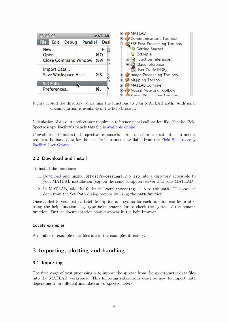
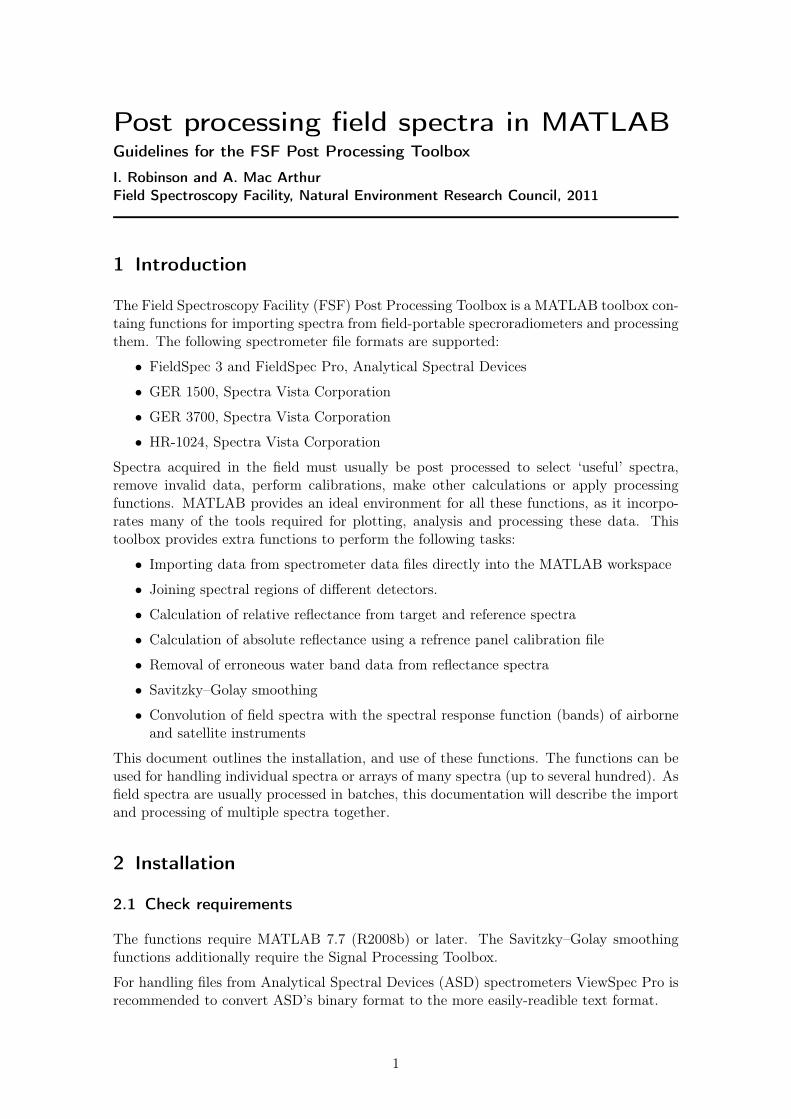
Figure 1: Add the directory containing the functions to your MATLAB path. Additionaldocumentation is available in the help broswer.

Calculation of absolute reflectance requires a reference panel calibration file. For the FieldSpectroscopy Facility’s panels this file is available online.

Convolution of spectra to the spectral response functions of airborne or satellite instrumentsrequires the band data for the specific instrument, available from the Field SpectroscopyFacility User Group.

2.2 Download and install

To install the functions:

1. Download and unzip FSFPostProcessing1.2.5.zip into a directory accessible toyour MATLAB installation (e.g. on the same computer/server that runs MATLAB).

2. In MATLAB, add the folder FSFPostProcessing1.2.5 to the path. This can bedone from the Set Path dialog box, or by using the path function.

Once added to your path a brief description and syntax for each function can be printedusing the help function; e.g. type help smooth for to check the syntax of the smoothfunction. Further documentation should appear in the help browser.

Locate examples

A number of example data files are in the examples directory.

3 Importing, plotting and handling

3.1 Importing

The first stage of post processing is to import the spectra from the spectrometer data filesinto the MATLAB workspace. This following subsections describe how to import datadepending from different manufacturers’ spectrometers.

2

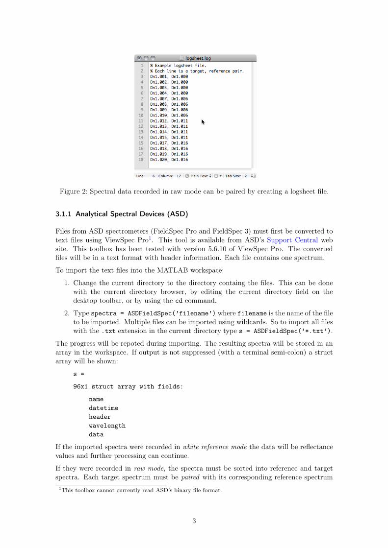
Figure 2: Spectral data recorded in raw mode can be paired by creating a logsheet file.

3.1.1 Analytical Spectral Devices (ASD)

Files from ASD spectrometers (FieldSpec Pro and FieldSpec 3) must first be converted totext files using ViewSpec Pro1. This tool is available from ASD’s Support Central website. This toolbox has been tested with version 5.6.10 of ViewSpec Pro. The convertedfiles will be in a text format with header information. Each file contains one spectrum.

To import the text files into the MATLAB workspace:

1. Change the current directory to the directory containg the files. This can be donewith the current directory browser, by editing the current directory field on thedesktop toolbar, or by using the cd command.

2. Type spectra = ASDFieldSpec(’filename’) where filename is the name of the fileto be imported. Multiple files can be imported using wildcards. So to import all fileswith the .txt extension in the current directory type s = ASDFieldSpec(’*.txt’).

The progress will be repoted during importing. The resulting spectra will be stored in anarray in the workspace. If output is not suppressed (with a terminal semi-colon) a structarray will be shown:

s =

96x1 struct array with fields:

namedatetimeheaderwavelengthdata

If the imported spectra were recorded in white reference mode the data will be reflectancevalues and further processing can continue.

If they were recorded in raw mode, the spectra must be sorted into reference and targetspectra. Each target spectrum must be paired with its corresponding reference spectrum

1This toolbox cannot currently read ASD’s binary file format.

3

using information from a logsheet recorded in the field. This information must be recordedin a separate text file. Figure 2 shows an example of a file called logsheet.log. Thisfile can be used to sort and pair the imported spectra by typing [tar, ref] = pair(s,’logsheet.log’). The original spectra will then be sorted and paired according to thepairings specified in the file:

tar =

1x16 struct array with fields:

namedatetimeheaderwavelengthdatapair

ref =

1x4 struct array with fields:

namedatetimeheaderwavelengthdata

Note that the target spectra have a field called pair which stores the name of the corre-sponding reference spectrum. This value is used later to calculate reflectance spectra.

3.1.2 Spectra Vista Corporation (SVC)

Files from SVC spectrometers (GER 1500, GER 3700 and HR-1024) are stored in thesignature format. This is a text format with header information. Each file contains twospectra: a target spectrum and a reference spectrum.

To import the text files into the MATLAB workspace:

1. Change the current directory to the directory containg the files. This can be donewith the current directory browser, by editing the current directory field on thedesktop toolbar, or by using the cd command.

2. Type [tar, ref] = SVCmodel(‘filename’) where model is the model of the spec-trometer and filename is the name of the file to be imported. Multiple files can beimported using wildcards. For example, to import spectra recorded on a GER1500spectrometer type [tar, ref] = SVCGER1500(‘*.sig’).

The progress will be repoted during importing. As each file contains a target spectrum anda reference specturm, the spectra are returned as two separate struct arrays for referenceand target spectra respectively:

tar =

1x7 struct array with fields:

namedatetime

4

headerpairwavelengthdata

ref =

1x7 struct array with fields:

namedatetimeheaderwavelengthdata

Note that the reference spectra may contain duplicates. This is because SVC signaturefiles always contain the previously-recorded reference spectrum for each target spectrum.

When importing spectra from models with multiple detectors, such as the HR-1024, theremay be overlapped data in the spectra. This occurs at the joins between the differentdetectors. The presence of overlapped data in imported spectra depends on the setting ofthe OverlapDataHandling.

Signature files from SVC instruments contain one target spectrum and its correspondingreference spectrum. Where the same reference spectrum is used for multiple target spec-trum there will therefore be multiple copies of the reference spectrum in different files.This will lead to duplicates in the structure array of reference spectra when imported.

3.2 Plotting

To plot a struct array s of spectra type plot([s.wavelength], [s.data]). This plotsspectral data columns againt a common set of wavelength values in the column vector w. .in the array. To plot an individual spectrum, say the sixth, type: plot(s(6).wavelength,s(6).data). To plot a range of spectra, say the second to the fourth (inclusive), type:plot([s(4:6).wavelength], [s(4:6).data]).

When plotting reflectance data, it may be preferable to multiply the data values by 100 toproduce a reflectance plot in per cent: plot([s.wavelength], 100*[s.data])

To change the horizontal scale from the default nanometres (nm) to micrometres (µm):plot(0.001*[s.wavelength], [s.data])

A legend can be added to the graph using MATLAB’s legend function. For example, toadd a legend showing the names of the spectra type: legend(spectra.name)

Axes labels, ranges and titles can be added using MATLAB’s built-in comands or the ploteditor. For example, the plot shown in Figure 3 was produced by typing:

plot([tar.wavelength], [tar.data]);legend(tar.name);xlabel(’Wavelength (nm)’);ylabel(’Intensity (a.u.)’);title(’Target spectra recorded on SVC GER 1500’);

5

200 300 400 500 600 700 800 900 1000 11000

2

4

6

8

10

12

14

16x 104

Wavelength (nm)

Inte

nsity

(a.u

.)

Target spectra recorded on SVC GER 1500

11−Jun−2010 12:52:3411−Jun−2010 12:52:4411−Jun−2010 12:53:3911−Jun−2010 12:53:5611−Jun−2010 12:54:5611−Jun−2010 12:55:0811−Jun−2010 12:55:33

Figure 3: Plot of seven target spectra from a SVC GER 1500 spectrometer.

3.3 Handling spectra

Imported data are stored in a MATLAB structure array. This ensures that importantheader information (such as the name, date and integration times) is kept together with thespectral data (wavelength and data). There are a number of ways to view and manipulatespectrum data in the workspace, described in the following subsections.

3.3.1 Structures

The spectra are stored as structures. A single spectrum would be a single structure,whereas multiple spectra are an array of structures (struct array).

The data are stored in the following fields:

• name is the name of the spectrum (usually taken from the filename)

• datetime is the date and time the spectrum was recorded2.

• header is a struct containing all the header information from the original file.

• pair appears only in target spectra from SVC data files. It gives the name of thecorresponding reference spectrum.

• wavelength is a column vector of wavelengths in nanometres.

• data is a column vector of the corresponding values. These will generally be uncal-ibrated digital numbers. For ASD spectrometers running in white reflectance modethese values will be reflectances in the range 0–1.

2The source of this data may be the spectrometer’s internal clock, or may be the clock of the computeror PDA used to record the spectrum.

6

Figure 4: Use the headers function to combine all headers into a single table.

3.3.2 Workspace browser

Open the workspace broswer by selecting Workspace from the Desktop menu, or typethe command workspace. The spectra will be visible as struct arrays with the namesgiven when imported. Double-click a struct array to browse its contents. If the strucurecontains multiple spectra, they will be listed as a row vector. Double-clock to open aspecific spectrum.

3.3.3 Listing fields

The fields of individual spectra can be viewed as a comma separated list. For example,typing s.name lists the names of all spectra in the structure ref.

>‌> s.name

ans =gr061110_000_reference

ans =gr061110_001_reference

...

Similarly, typing s.header lists the headers of all spectra.

Whilst this is practical when working with a few spectra, for large numbers of spectra itwill produce too much output. Instead data can be rearranged to a more suitable formatas described in the following subsections.

3.3.4 Creating a table of header information

A function called headers provides a method to copy all header information into a single(large) cell array. For example, typing H = headers(s) will create a cell array H containing

7

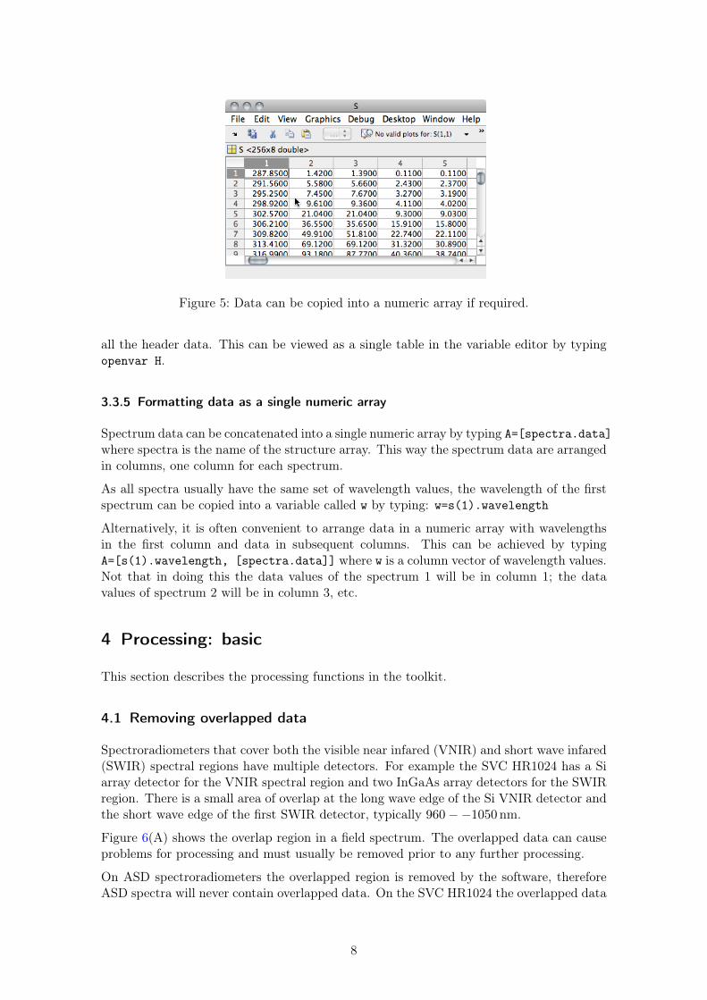
Figure 5: Data can be copied into a numeric array if required.

all the header data. This can be viewed as a single table in the variable editor by typingopenvar H.

3.3.5 Formatting data as a single numeric array

Spectrum data can be concatenated into a single numeric array by typing A=[spectra.data]where spectra is the name of the structure array. This way the spectrum data are arrangedin columns, one column for each spectrum.

As all spectra usually have the same set of wavelength values, the wavelength of the firstspectrum can be copied into a variable called w by typing: w=s(1).wavelength

Alternatively, it is often convenient to arrange data in a numeric array with wavelengthsin the first column and data in subsequent columns. This can be achieved by typingA=[s(1).wavelength, [spectra.data]] where w is a column vector of wavelength values.Not that in doing this the data values of the spectrum 1 will be in column 1; the datavalues of spectrum 2 will be in column 3, etc.

4 Processing: basic

This section describes the processing functions in the toolkit.

4.1 Removing overlapped data

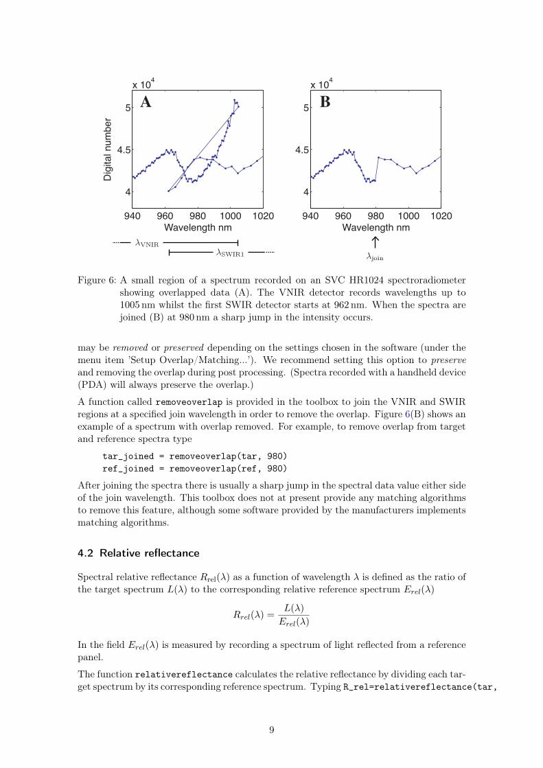
Spectroradiometers that cover both the visible near infared (VNIR) and short wave infared(SWIR) spectral regions have multiple detectors. For example the SVC HR1024 has a Siarray detector for the VNIR spectral region and two InGaAs array detectors for the SWIRregion. There is a small area of overlap at the long wave edge of the Si VNIR detector andthe short wave edge of the first SWIR detector, typically 960−−1050 nm.

Figure 6(A) shows the overlap region in a field spectrum. The overlapped data can causeproblems for processing and must usually be removed prior to any further processing.

On ASD spectroradiometers the overlapped region is removed by the software, thereforeASD spectra will never contain overlapped data. On the SVC HR1024 the overlapped data

8

940 960 980 1000 1020

4

4.5

5

x 104

Wavelength nm

Dig

ital n

umbe

r

940 960 980 1000 1020

4

4.5

5

x 104

Wavelength nm

A B

Figure 6: A small region of a spectrum recorded on an SVC HR1024 spectroradiometershowing overlapped data (A). The VNIR detector records wavelengths up to1005 nm whilst the first SWIR detector starts at 962 nm. When the spectra arejoined (B) at 980 nm a sharp jump in the intensity occurs.

may be removed or preserved depending on the settings chosen in the software (under themenu item ’Setup Overlap/Matching...’). We recommend setting this option to preserveand removing the overlap during post processing. (Spectra recorded with a handheld device(PDA) will always preserve the overlap.)

A function called removeoverlap is provided in the toolbox to join the VNIR and SWIRregions at a specified join wavelength in order to remove the overlap. Figure 6(B) shows anexample of a spectrum with overlap removed. For example, to remove overlap from targetand reference spectra type

tar_joined = removeoverlap(tar, 980)ref_joined = removeoverlap(ref, 980)

After joining the spectra there is usually a sharp jump in the spectral data value either sideof the join wavelength. This toolbox does not at present provide any matching algorithmsto remove this feature, although some software provided by the manufacturers implementsmatching algorithms.

4.2 Relative reflectance

Spectral relative reflectance Rrel(λ) as a function of wavelength λ is defined as the ratio ofthe target spectrum L(λ) to the corresponding relative reference spectrum Erel(λ)

Rrel(λ) =L(λ)

Erel(λ)

In the field Erel(λ) is measured by recording a spectrum of light reflected from a referencepanel.

The function relativereflectance calculates the relative reflectance by dividing each tar-get spectrum by its corresponding reference spectrum. Typing R_rel=relativereflectance(tar,

9

ref) calculates relative reflectance spectra from the target spectra tar and reference spec-tra ref. Each spectrum in the struct array tar must have a field called pair which definesthe corresponding reference spectrum in the series ref.

4.3 Absolute reflectance

Absolute spectral reflectance Rabs(λ) as a function of wavelength λ is the ratio of the targetspectrum L to the spectral irradiance E(λ). However, in the field it is usually the relativereference spectrum Erel(λ) which is measured. This is the spectral irradiance which isreflected by the panel

Erel(λ) = Rpanel(λ)E(λ)

where Rpanel(λ) is the spectral reflectance of the panel.

The absolute reflectance can be calculated from the relative reflectance

Rabs(λ) =L(λ)

E(λ)= Rpanel(λ)

L(λ)

Erel(λ)= Rpanel(λ)Rrel(λ)

Therefore to convert absolute reflectance to relative reflectance the spectrum must bemultiplied by the reflectance of the panel that was used to record it. The panel reflectancedata are provided by a panel calibration file which records the panel reflectance over a setof wavelengths Rpanel(λ). If the calibration file is recorded with the same spectrometer asthe field spectrum the set of wavelengths λ will be the same for both spectrum and panel.Otherwise the panel spectrum must be interpolated to the wavelengths of the relativereflectance spectrum.

Panel calibration files can be provided in one of two formats:

1. A comma-separated values (CSV) file with a header that gives some metadata aboutthe panel.

2. An Excel spreadsheet downloaded form the Field Spectroscopy Facility’s web siteweb site (for the Facility’s panels).

For a file in CSV format, the file format is as follows:

rt the panel calibration file type

Panel calibration file for FSF Post Processing ToolboxName: SRT #011Date of calibration: 2011-04-03350,0.980351,0.980352,0.981

...and so on. The first column is wavelength and the second is reflectance (in the range0–1). Noe that the header data is required.

To import the panel calibration from a CSV file type

p = importpanelcalibration(’panel.csv’)

From an Excel spreadsheet the serial number of the panel must also be specified

P = importpanelcalibration(’FSF Ref Panel Cal Data 2010_1.xls’, ’SRT#008’)

10

MATLAB may give several warnings when importing an Excel spreadsheet. However ifthe import is successful these may be ignored.

The panel calibration spectrum can be plotted

plot(P.wavelength, P.data)

Once panel data are loaded, the absolute reflectance can be calculated using the functionabsolutereflectance. Typing

R_abs=absolutereflectance(R_rel, P)

calculates the absolute reflectance from the struct array or relative reflectance spectrumusing the panel calibration data in the specified spreadsheet. ’SERIAL’ is the serial numberof the panel, e.g. ’SRT #004’.

Once calculated, absolute reflectance can be plotted using MATLAB’s plot function. Re-flectance values are (normally) in the range 0–1. A graph of reflectance as a percentagecan be plotted by multiplying the reflectance values by 100:

plot([R_abs.wavelength], 100*[R_abs.data]);legend(R_abs.name);xlabel(’Wavelength (nm)’);ylabel(’Absolute reflectance (%)’);title(’Reflectance spectra recorded on SVC GER 1500’);

4.4 Smoothing

The function smooth smooths spectra with Savitzky–Golay smoothing [1]. Typing S=sgsmooth(R_abs)smooths a struct array of spectra R_abs, returning a struct array of smoothed spectra S.The smoothing reduces the wavelength range of the spectra, so the spectra in S will havea new wavelength scale.

4.5 Removing water bands

The function removewater deletes data in the water band regions which are usually erro-neous. Type W=removewater(S) to delete water bands from a struct array S, returning anew struct array W.

The data points are removed by replacing them with the special value not a number (NaN).This special value is used to indicate that data have been removed. Further processing ofdata in this region causes NaN.

5 Processing: advanced

5.1 Convolution

The function convolve provides a means to convolve a spectrum [2] or spectra with thespectral response functions of airborne or satellite instruments. This procedure is used tocompare data from high-resolution field-portable spectroradiometers with lower-resolutioninstruments.

11

The first step in this processing function is to download the spectral response functions(bands) for the specific instrument. These data are provided as XML files and are listedon the Field Spectroscopy Facility’s web site.

The class Band can be used to load response data into MATLAB. For example, to loadspectral response data for the POLDER instrument type

POLDER = Band(’http://fsf.nerc.ac.uk/user_group/bands/POLDER.xml’)

By default the response data are normalized such that the area under each curve is 1. ThenormalizeHeight method can be used to normalize such that the height of each responsefunction is 1:

POLDER.plotPOLDER.normalizeHeight.plot

To convolve with a spectrum S, type

T = convolve(S, POLDER)

If the spectrum S and the bands POLDER are defined on different wavelength scales, thebands will be interpolated.

To plot the output spectrum T

plot(T.wavelength, T.data)

Note that the convolve function cannot be used on spectra where there are overlappingdata.

5.2 Feature depth estimation

The depth of an absorption feature in a spectrum can be estimated using the methoddescribed by Clark and Roush [3]. The function featuredepth provides an illustration ofthe method.

References

[1] Savitzky, Abraham and Golay, M J E, “Smoothing and Differentiation of Data bySimplified Least Squares Procedures.” Analytical Chemistry, volume 36, no. 8, pp. 1627–1639, 1964

[2] James, J F, Spectrograph Design Fundamentals, Cambridge University Press, 2007

[3] Clark, R N and Roush, T L, “Reflectance spectroscopy: quantitative analysis techniquesfor remote sensing applications,” J Geophys Res, volume 89, p. 6329, 1984

Appendix: normalization of ASD spectra in raw mode

ASD spectra recorded in raw mode must be normalized to account for the different re-sponses of the detectors. The normalization is performed during import and the code iscontained in the function ASDFieldSpec. (Reflectance spectra recorded in white referencemode are not normalized.)

12

The ASD FieldSpec 3 and FieldSpec Pro spectroradiometers have three separate detectorsfor three different spectral regions. A silicon photodiode array detects light in the visible-near-infrared (VNIR) region. Two InGaAs photodiodes cover two short wave infraredspectral regions labelled SWIR1 and SWIR2.

VNIR SWIR1 SWIR2

λ1 and λ2 are the join wavelengths. These may be different for different instruments, butthe values are saved in ASD spectrum files. They can be found in the header structure infields named Join1Wavelength and Join2Wavelength.

The pixel values DN are normalized differently in each spectral region:

DNnorm(λ) =

DN(λ)TVNIR

λ 6 λ1GSWIR1DN(λ)

2048 λ1 < λ 6 λ2GSWIR2DN(λ)

2048 λ2 < λ

where TVNIR is the integration time of the VNIR photodiode array, GSWIR1 is the gain ofthe SWIR1 photodiode and GSWIR2 is the gain of the SWIR2 photodiode. These values aresaved in ASD spectrum files, and are imported into the MATLAB workspace as fields in theheader structure called VNIRIntegrationTime, SWIR1Gain and SWIR2Gain respectively.

13