Portfolio Optimization with an

Envelope-based Multi-objective Evolutionary Algorithm

J. Branke1, B. Scheckenbach1,2, M. Stein1, K. Deb3, H. Schmeck1

1 Institute AIFB, University of Karlsruhe, Germany

2 SAP AG, Walldorf, Germany

3 Kanpur Institute of Technology, India

Abstract

The problem of portfolio selection is a standard problem in financial engineering and has

received a lot of attention in recent decades. Classical mean-variance portfolio selection aims

at simultaneously maximizing the expected return of the portfolio and minimizing portfolio

variance. In the case of linear constraints, the problem can be solved efficiently by parametric

quadratic programming (i.e., variants of Markowitz’ critical line algorithm). However, there

are many real-world constraints that lead to a non-convex search space, e.g. cardinality

constraints which limit the number of different assets in a portfolio, or minimum buy-in

thresholds. As a consequence, the efficient approaches for the convex problem can no longer

be applied, and new solutions are needed.

In this paper, we propose to integrate an active set algorithm optimized for portfolio

selection into a multi-objective evolutionary algorithm (MOEA). The idea is to let the MOEA

come up with some convex subsets of the set of all feasible portfolios, solve a critical line

algorithm for each subset, and then merge the partial solutions to form the solution of the

original non-convex problem. We show that the resulting envelope-based MOEA significantly

outperforms existing MOEAs.

1

1 Introduction

In finance, a portfolio is a collection of assets held by an institution or a private individual. The

portfolio selection problem seeks an optimal way to distribute a given budget on a set of available

assets.

The problem usually has two criteria: Expected return (mean profit) is to be maximized, while

the risk is to be minimized. The optimal solution depends on the user’s risk aversion. As it is

often difficult to weigh the two criteria before the alternatives are known, it is common to search

for the whole set of efficient or Pareto-optimal solutions, i.e. all solutions that can not be improved

upon in both objectives simultaneously. This set of solutions is often called “efficient frontier”,

or “Pareto-optimal front”. Another motivation for searching for the whole efficient frontier stems

from the fact that in many applications, a set of solutions with different trade-offs with respect

to the optimization criteria are desired, e.g. because a bank wants to offer its customers different

choices depending on their risk aversion.

A natural measure for risk is the variance of the portfolio return. Mean-variance optimization

is probably the most popular approach to portfolio selection. It was introduced more than 50

years ago in the pioneering work by Markowitz (1952, 1956). The basic assumptions in his theory

are a rational investor with either multivariate normally distributed asset returns or, in the case of

arbitrary returns, a quadratic utility function (Huang and Litzenberger, 1988). It has been shown

that if these assumptions are valid, the optimal portfolio for the investor lies on the mean-variance

efficient frontier.

The basic mean-variance portfolio selection problem we consider in this paper can be formalized

as follows:

min V (w) = wT Qw (minimize portfolio variance) (1a)

max wT µ = E (maximize expected return) (1b)

subject to

wT e = 1 (budget constraint) (1c)

0 ≤ wi ≤ 1 i = 1, . . . , N (1d)

where N is the number of assets to choose from, Q denotes the covariance matrix of all

investment alternatives, µi is the expected return of asset i, and e is the unit vector. The decision

2

variables wi determine what share of the budget should be distributed to asset i, and Eq.1c makes

sure that the sum of all wi is equal to one, i.e. that the whole budget is invested.

Computationally efficient algorithms that calculate a single point or even the whole efficient

frontier of this basic portfolio selection problem have been discussed in a large number of publi-

cations. For a basic introduction to portfolio selection see e.g. Elton et al. (2003). The algorithm

to compute the whole efficient frontier (critical line algorithm) is described in detail in Markowitz

(1987). The result of this algorithm is a sequence of so-called corner portfolios. These cor-

ner portfolios define the complete efficient frontier as all other points on the frontier are convex

combinations of the two adjacent corner portfolios.

However, these highly efficient algorithms can not take into account more complex constraints

that lead to a non-convex search space, henceforth called non-convex constraints. Examples for

such constraints which are commonly used in mutual fund management include:

1. Cardinality constraints restrict the number of securities which are allowed in the portfolio.

Often, the maximal number of securities in the portfolio is limited to reduce the management

cost e.g. for monitoring the performance of the companies in the portfolio.

2. The 5-10-40 constraint is based on §60(1) of the German investment law (InvG, 2004).

It defines an upper limit for each individual asset and for the sum of all “heavyweights” in

the portfolio. More specifically, securities of the same issuer are allowed to amount to 5% of

the net asset value of the mutual fund. They are allowed to amount to 10%, however, if the

total share of all assets with a share between 5% and 10% is less than 40% of the net asset

value.

3. Buy-in thresholds demand that if an asset is included in the portfolio, at least some

amount l should be bought. The main reason for such a constraint is to reduce transaction

costs. In principle, this constraint could also be handled by our approach in a straightforward

manner, but is not considered further in this paper.

For convex portfolio selection problems, the critical line algorithm is able to generate the com-

plete (continuous) efficient frontier. In the presence of non-convex constraints, most approaches

found in the literature are based on the ε-constraint method (see e.g. Miettinen (1998)): Instead

of optimizing both criteria simultaneously, they set the expected return to a constant (i.e. Eq. 1b

3

becomes a constraint), and solve the resulting quadratic optimization problem to minimize the

variance. Of course, this only generates a single solution on the efficient frontier, and the algorithm

has to be applied many times with different expected returns to obtain a reasonable approxima-

tion of the true efficient frontier. Furthermore, as the solution of each quadratic sub-problem is

computationally complex in the presence of non-convex constraints1, usually heuristics are used

to solve the individual sub-problems, which means that the generated solutions don’t necessarily

lie on the true efficient frontier. Some heuristic approaches like evolutionary algorithms allow to

consider multiple objectives simultaneously, generating a set of solutions approximating the effi-

cient frontier in one run. However, they are still point-based, generating a finite set of alternative

portfolios.

In this paper, we propose to combine multi-objective evolutionary algorithms with an em-

bedded critical line algorithm to solve complex portfolio selection problems with non-convex con-

straints. The basic idea is to let the EA handle the non-convex constraints and to basically divide

the problem into a set of problems with convex constraints, which can be solved optimally with a

critical line algorithm. The overall solution to the problem is then the combination of the solutions

to the individual convex problems. As we will demonstrate, the approach significantly outper-

forms other state-of-the-art evolutionary algorithms. Furthermore, to our knowledge, this is the

first approach to non-convex portfolio selection yielding a continuous solution set, as opposed to

the discrete solution set generated by the point based approaches.

Our paper is structured as follows. First, we provide a brief overview on approaches to portfolio

selection subject to non-convex constraints. A short introduction to multi-objective evolutionary

algorithms is provided in Section 3, followed in Section 4 by a short description of a state-of-the-art

point-based MOEA which will be used as a reference later on. Our approach, called envelope-based

multi-objective evolutionary algorithm (E-MOEA) is presented in Section 5. Section 6 reports on

the empirical evaluation of our approach. The paper concludes in Section 7 with a summary and

some ideas for future work.

1In fact, some variants are NP-complete, e.g. the cardinality constrained portfolios if the maximum cardinality

is a fraction of the total number of assets (Bienstock, 1996)

4

2 Related work

The work on non-convex portfolio selection problems can be roughly divided into mixed integer

approaches and metaheuristics which will be discussed in turn.

2.1 Mixed Integer Approaches

By adding integer variables, the convex problem presented in the previous section can be extended

to take non-convex constraints into account. For example, buy-in thresholds and cardinality

constraints can be modeled as follows:

min V (w) = wT Qw (2a)

subject to

wT µ = E (2b)

wT e = 1 (2c)

n∑i=1

ρi ≤ N (2d)

lρi ≤ wi ≤ uρi i = 1, . . . , N (2e)

ρi ∈0, 1 i = 1 . . . N (2f)

where ρi is the binary variable that specifies whether asset i should be included in the portfolio,

and l and u are the lower and upper bounds for the weights if the corresponding asset is included.

The modelling of the 5-10-40 constraint as MIQP is not as straightforward, and requires to

5

triple the number of variables:

min V (w) = wT Qw (3a)

subject to

wT µ = E (3b)

wT e = 1 (3c)

w − 0.05ρ ≤ 0.05e (3d)

t− 0.1ρ ≤ 0 (3e)

t−w ≤ 0 (3f)

w + 0.1ρ− t ≤ 0.1e (3g)

tT e ≤ 0.4 (3h)

w, t ≥ 0 (3i)

ρi ∈0, 1 i = 1, . . . , N (3j)

Thereby, ρi = 1 implies that asset i is allowed up to 10%, while ρi = 0 restricts asset i to

5%. If ρi = 0, Inequality 3e requires ti = 0, otherwise ti = wi by Inequalities 3e, 3f, and 3g.

Inequalities 3h and 3i restrict the “heavyweights” to 10% and their sum to 40%.

Once formulated appropriately, any of the available mixed integer quadratic programming

(MIQP) solvers can be used to solve the model. Software packages that contain such a solver

can be found at NEOS Guide (2006), although – compared to the number of available QP-

solvers – there are by far fewer programs with the required capability. In any case, there is

no guarantee for getting the optimal portfolio quickly. If there is not enough time to allow the

algorithm to terminate regularly, the best valid portfolio calculated so far can be used instead — a

normal practice when working with mixed integer solvers. Of course, this abandons the optimality

guarantee.

For further information about the mixed integer approach to the cardinality constrained prob-

lem without using an external MIQP-solver, the reader is referred to Bienstock (1996). Bienstock

examined the computational complexity of the problem, tested a self-developed branch-and-cut

algorithm using disjunctive cuts, and discussed some of the implementation problems that oc-

curred.

Jobst et al. (2001) use a branch-and-bound algorithm to solve the cardinality constrained

6

problem with buy-in thresholds as well as an index tracking problem, where a portfolio subject

to cardinality constraints should perform as closely as possible to an index in terms of mean and

variance. As they calculate many points on the efficient frontier, the available time is too short

for individually solving each MIQP to optimality. Therefore, they limit the number of nodes in

the search tree of the branch-and-bound algorithm for each given expected return E. To speed

up the algorithm further, a previously calculated solution for an adjacent point is used as a warm

start solution for the new value of expected return.

Advantages of the mixed integer approaches are certainly that optimality is guaranteed if the

algorithm terminates. On the other hand, running time is difficult to predict, and modelling

complex constraints is not always straightforward. Finally, the efficient frontier can only be

calculated pointwise, a mixed integer version of the critical line algorithm is not known.

2.2 Metaheuristics

Because of the potentially extensive running times of the mixed integer approaches and their

complex implementation, many researchers have turned to metaheuristics. The term metaheuristic

usually describes a generic optimization principle that is widely applicable to many different

problem domains. Very often, the basic idea behind a metaheuristic is inspired by nature, be it a

physical process like simulated annealing (SA) or biologically inspired algorithms like ant colony

optimization (ACO) or evolutionary algorithms (EAs). Such metaheuristics do not guarantee

optimality, but it is hoped that they find reasonable solutions quickly.

There are several publications discussing the use of metaheuristics to solve non-convex portfolio

selection problems. Most of them apply the metaheuristic just to solve the MIQP with a given

desired expected return, i.e. to generate a single point of the efficient frontier in mean-variance

objective space.

Chang et al. (2000) compare an EA, tabu search, and SA to solve portfolio selection problems

where each solution has to contain a predetermined number of assets. Because none of the ap-

proaches turned out to be a clear winner, they suggest to run all three and combine the results.

Schaerf (2002) improves on the work of Chang et al. by testing several neighborhood relations for

tabu search. Crama and Schyns (2003) apply simulated annealing to a portfolio selection problem

with cardinality constraints as well as turnover and trading restrictions. They particularly focused

7

on ways to handle constraints, partially by enforcing feasibility, partially by introducing penalties.

A hybrid between SA and EA is proposed in Maringer and Kellerer (2003). In Maringer (2002),

ACO is used only to determine the relevant assets for a cardinality-constrained portfolio selection

problem, while the weights are determined with a conventional QP solver. The only authors who,

to our knowledge, address the 5-10-40 constraint are Derigs and Nickel (2001). They use SA for

optimization, but do not provide details on how they ensure feasibility of solutions. In Derigs

and Nickel (2003), they expand their previous work, but the focus is put on developing a decision

support system for portfolio selection. In Ehrgott et al. (2004), a problem with five objectives and

non-convex constraints is considered, but the five objectives are accumulated into one based on

multiattribute utility theory. Then local search, SA, tabu search and an EA are used to solve the

resulting single-objective mixed-integer problem.

Eddelbuttel (1996) uses a QP solver within a genetic algorithm to solve the index-tracking

problem. Here, the GA determines which assets should be included in the portfolio, while the

optimal weights are calculated by the QP solver.

Instead of setting the expected return E as constant and then solving a separate single-objective

optimization problem for several E as do all of the above methods, Streichert et al. (2003, 2004a,b),

apply a multi-objective evolutionary algorithm (MOEA). MOEAs are variants of EAs that exploit

the fact that EAs work with a population of solutions, and simultaneously search for a set of

efficient alternatives in a multi-objective setting, see also the following section. Note that while

this approach generates several solutions along the efficient frontier in one run, it is still point-

based (i.e. it only generates a discrete set of solutions). Since we will use this algorithm for

empirical comparison with our approach, it will be discussed in more depth below.

Other publications reporting on the use of MOEAs for portfolio selection include Lin and Wang

(2002) who consider roundlots2, and Fieldsend et al. (2004), who address the cardinality issue but

consider the number of allowed assets, K, as a third objective to be minimized. Armananzas and

Lozano (2005) apply multi-objective variants of greedy search, SA and ACO to the cardinality-

constrained portfolio selection problem. Schlottmann and Seese (2005) consider credit portfolio

optimization and use a gradient-based local search within their MOEA.

General advantages of metaheuristic approaches are certainly their flexibility. It would be

2In a portfolio selection problem with roundlots, an asset can only be bought in multiples of a minimum lot.

This problem has been proven to be NP-complete.

8

straightforward e.g. to use alternative, risk measures. Also, the multi-objective versions allow to

generate a whole set of solutions, approximating the efficient frontier with a single run.

3 Multi-objective evolutionary algorithms

Although a detailed introduction into multi-objective evolutionary algorithms (MOEAs) would

exceed the scope of this paper, in this section we will briefly introduce the main ideas which are

needed as foundation for the subsequent sections. For a more detailed introduction to MOEAs,

the reader is referred to Deb (2001) or Coello et al. (2002). A survey on MOEA applications in

finance can be found in Schlottmann and Seese (2004).

Evolutionary algorithms are stochastic iterative optimization heuristics inspired by natural

evolution. Starting with a set of candidate solutions (population), in each iteration (generation),

promising solutions are selected as potential parents (mating selection), and new solutions (indi-

viduals) are created by mixing information from the parents (crossover) and slightly modifying

them (mutation). The resulting offspring are then inserted into the population, replacing some

old or less fit solutions (environmental selection). By continually selecting good solutions for re-

production and then creating new solutions based on the knowledge represented in the selected

individuals, the solutions “evolve” and become better and better adapted to the problem to be

solved, just like in nature, where the individuals become better and better adapted to their envi-

ronment through the means of evolution.

The basic operations of an evolutionary algorithm can be described as follows:

t := 0

initialize P (0)

evaluate P (0)

WHILE (termination criterion not fulfilled) DO

copy selected individuals into mating pool: M(t) := s(P (t))

crossover: M ′(t) := c(M(t))

mutation: M ′′(t) := m(M ′(t))

evaluate M ′′(t)

update population: P (t + 1) := u(P (t) ∪M ′′(t))

9

t := t + 1

DONE

with t denoting the generation counter, P (t) the population at generation t, and s, c, m, and

u representing the different genetic operators. Evolutionary algorithms have proven successful in

a wide variety of applications. For a more detailed introduction to EAs, the reader is referred to

Eiben and Smith (2003).

Because EAs maintain a population of solutions throughout the run, they can also be used to

simultaneously search for a set of solutions approximating the efficient frontier of a multi-objective

problem.

The main difference between single objective EAs and MOEAs is the way they rank their

solutions for selection. While in single objective EAs the ranking is unambiguously defined by the

solution quality, this is not so straightforward in the case of multiple objectives. MOEAs have

two goals: they want to drive the population towards the efficient frontier, while at the same

time maintaining a diverse set of alternative solutions. To achieve the first goal, most MOEA

implementations rely on the concept of dominance. Solution A dominates solution B if A is at

least as good as B in all objectives, and better in at least one objective. A solution is called

non-dominated with respect to a set of solutions if and only if it is not dominated by any other

solution in that set.

One particularly popular MOEA variant is the non-dominated sorting genetic algorithm (NSGA-

II), see Deb (2001). It ranks individuals according to two criteria. First, individuals are ranked

according to non-dominancy: All non-dominated individuals are assigned to Front 1, then they are

removed from the population, again all non-dominated solutions are determined and are assigned

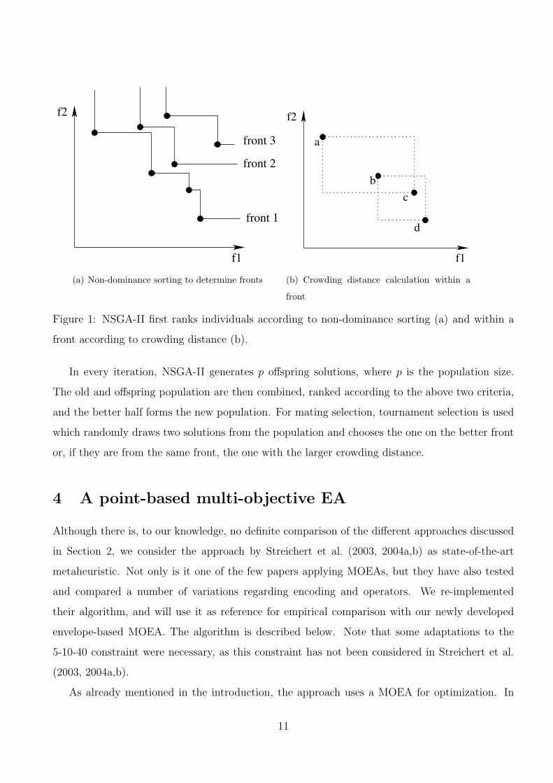
Front 2, etc. until the population is empty. The result of this process is illustrated in Figure 1(a).

Within a front, solutions are ranked according to the crowding distance, which is defined as the

circumference of the rectangle defined by their left and right neighbors, and infinity if there is

no neighbor. This concept is illustrated in Figure 1(b). Individuals with high crowding distance

are preferred, as they are in more isolated regions of the objective space. In the example in Fig-

ure 1(b), individuals a and d have the highest priority within the front, followed by individual b

and then c because the rectangle defined by the respective left and right neighbor is larger for

individual b.

10

f1

f2

front 3

front 1

front 2

(a) Non-dominance sorting to determine fronts

f1

f2

a

b

c

d

(b) Crowding distance calculation within a

front

Figure 1: NSGA-II first ranks individuals according to non-dominance sorting (a) and within a

front according to crowding distance (b).

In every iteration, NSGA-II generates p offspring solutions, where p is the population size.

The old and offspring population are then combined, ranked according to the above two criteria,

and the better half forms the new population. For mating selection, tournament selection is used

which randomly draws two solutions from the population and chooses the one on the better front

or, if they are from the same front, the one with the larger crowding distance.

4 A point-based multi-objective EA

Although there is, to our knowledge, no definite comparison of the different approaches discussed

in Section 2, we consider the approach by Streichert et al. (2003, 2004a,b) as state-of-the-art

metaheuristic. Not only is it one of the few papers applying MOEAs, but they have also tested

and compared a number of variations regarding encoding and operators. We re-implemented

their algorithm, and will use it as reference for empirical comparison with our newly developed

envelope-based MOEA. The algorithm is described below. Note that some adaptations to the

5-10-40 constraint were necessary, as this constraint has not been considered in Streichert et al.

(2003, 2004a,b).

As already mentioned in the introduction, the approach uses a MOEA for optimization. In

11

particular, it is based on the standard non-dominated sorting genetic algorithm (NSGA-II and its

predecessor NSGA) as described above.

As genetic representation, Streichert et al. (2003, 2004a,b) recommend to use a hybrid binary/real-

valued encoding, which is also used by several other successful approaches like Chang et al. (2000).

With this encoding, a solution is defined by a vector of continuous variables c = (c1, . . . , cN)T

representing the weights of the individual assets. An additional vector of binary variables k =

(k1, . . . , kN)T is used to indicate if the asset is included in the portfolio at all. The latter vector

allows the EA to easily add or remove an asset by simply flipping the corresponding bit, and thus

facilitates the handling of cardinality constraints.

For a portfolio selection problem that contains a cardinality constraint and buy-in thresholds,

the decoding of the two vectors to get the actual portfolio works as follows (see e.g. Chang et al.

(2000); Streichert et al. (2004a)):

1. All ci are set to zero if ki = 0.

2. If∑N

i=1 sign(kici) is more or less than the required cardinality, the solution is repaired by

changing some elements of c. For the maximum cardinality problem, elements are set to 0

in the order of increasing ci (i.e. the assets with the smallest share are set to zero).

3. The vector c is normalized:

c′i =ci∑ci

(4)

4. The final weight wi is calculated:

wi =

l + c′i (1− |Υ|l) if i ∈ Υ

0 otherwise(5)

where l is the minimum buy-in threshold and |Υ| denotes the number of elements in Υ.

The 5-10-40 constraint has not yet been considered by Streichert et al., and thus we had to

adapt the decoding and repair mechanism. It works in 7 steps as follows.

1. All ci are set to zero if ki = 0.

2. The vector c is normalized:

wi =ci∑ci

12

3. The surplus amount exceeding the 10% threshold is calculated, Ω =∑

wi>0.1

(wi − 0.1). All

wi > 0.1 are set to 0.1.

4. the surplus Ω has to be redistributed to the weights below 10%. Each weight below 10% is

raised by the amount (0.1− wi) · ΩΨ, where Ψ =

∑0<wi<0.1

(0.1− wi). If Ψ < Ω, no weight will

have a value above 10% after the first step.

5. In the group with more than 5%, we only accept the assets with the largest weights such

that the sum is still less than or equal to 40%. All others are capped to 5% and the excess

weight is distributed to the the other assets analogously to the above step.

6. If there is not enough room for all the excess weight to be redistributed among the assets

with less than 5%, the remaining is used to fill up the assets between 5% and 10% up to

10% in order of decreasing weight.

7. The previous step may again lead to a violation of the 5-10-40 constraint. In this case, assets

are removed from the 5-10% group in order of increasing weights, and the weight in excess

of 5% is distributed to the other assets in the 5-10% group similar to the previous step.

Note that any valid portfolio for the problem with 5-10-40 constraint contains at least 16

different assets (4 times 10% plus 12 times 5%). If this is the case, the above decoding will result

in a feasible portfolio. By appropriate mutation and crossover operators (see below) we make sure

that the binary string has always at least 16 bits set to “1”.

For both cardinality constraints and the 5-10-40 constraint, the weights after the above repair

steps are written back into the weight-vector of the genotype and overwrite the original values.

This allows the information gained by the repair mechanism to be inherited to the offspring

(Lamarckism) and has been recommended in Streichert et al. (2004b).

For mutation, simple bit flip is used on the binary vector, and Gaussian mutation on the

real-valued vector. For crossover, we use N-point crossover independently on both real-valued and

binary vector. In Streichert et al. (2004a), this crossover operator was reported to be competitive to

other, more complex crossover operators. We follow this suggestion for the cardinality constrained

problem. For the 5-10-40 constraint, as explained above, we need at least 16 assets with ki = 1

for a feasible solution. Therefore, for this constraint we modify the operators on the bit string as

13

follows. The crossover operator first transfers all bits to the child where both parents are equal.

The remaining bits are traversed in random order and randomly taken from either parent until

the maximum number of zeros has been reached (i.e. N − 16 if N is the number of assets). Any

remaining bits are set to 1. If after mutation the resulting bit string contains less than 16 ones,

some of the performed 1 to 0 bit flips are reversed to make the string valid.

In the remainder of this paper, we will denote this point-based MOEA as P-MOEA.

5 Envelope-based multi-objective evolutionary algorithm

In this section, we will present our new envelope-based multi-objective evolutionary algorithm (E-

MOEA) for portfolio selection problems. It combines the efficiency of the critical line algorithm for

calculating the whole continuous front with the ability of multi-objective evolutionary algorithms

to take complex constraints into account and to generate multiple solutions within a single run.

The main idea of our paper is to use the MOEA to define suitable convex subsets of the original

search space, run the critical line algorithm on every subset, and then recombine the partial

solutions to form the complete front.

A single solution (individual of the MOEA) defines a convex subset by specifying how the

non-convex constraints are to be handled. In case of a cardinality constraint, a solution defines

which assets are allowed a weight greater than zero. The corresponding convex problem is just the

standard problem which contains only those variables not forced to zero. Note that, in particular

if the allowed cardinality is much smaller than the total number of available assets, this means

that the generated sub-problem is much smaller than the original problem, which results in a

tremendous reduction of the running time of the critical line algorithm.

For the case of the 5-10-40 constraint, a solution defines which assets are allowed up to 10%

and hence have to be included in the 40% constraint. All other assets are restricted to at most

5%.

For each subset, the critical line algorithm can be used to efficiently calculate the whole efficient

frontier of the corresponding standard mean-variance portfolio selection problem. For more details

to the critical line algorithm, the reader is referred to Markowitz (1987). Because we apply the

critical line algorithm to every individual generated by the EA, an efficient implementation is

crucial. We use a modified variant of the algorithm described by Best, M. J. and Kale, J. K.

14

(2000). For an in-depth discussion of implementation intricacies see Stein et al. (2006).

The result of the critical line algorithm is a front in the mean-variance space which is efficient

for the sub-problem, but not necessarily for the overall problem with non-convex constraints. We

call such a partial front an envelope. The EA is now used to find a collection of such envelopes

which together form a solution to the overall problem.

For this purpose, we use a multi-objective EA based also on the general framework of NSGA-II

(Deb, 2001). But instead of a solution being represented by a single point in the mean-variance

space, now every solution is represented by an envelope in the mean-variance space. An exemplary

population is depicted in Figure 2(a). The example shows that situations where envelopes entirely

dominate other envelopes occur very rarely. Instead, at many points, envelopes intersect with

other envelopes. Even without intersections, many envelopes have dominated and non-dominated

parts. Thus, we had to adapt the non-dominated sorting and crowding distance calculation to

work with envelopes. The basic idea can be described as follows.

We are interested in the non-dominated part of the set union of all envelopes. Let us denote

the non-dominated part of the unit set of all envelopes as (first) aggregated front. Following the

idea of non-dominated sorting, we assign Rank 1 to all individuals contributing at least partially

to the first aggregated front. Then, we iteratively remove these individuals/envelopes from the

population, and determine the aggregated front of the remaining individuals, assigning them the

next higher rank, etc. The resulting ranking and the generated aggregated fronts are depicted in

Figure 2(b).

It is clear that different individuals contribute differently to an aggregated front. Some may

contribute only a small segment of the front, some may contribute large segments. Also, some

parts of the aggregated front may be represented by several individuals. We use this information

to rank the individuals within a front (substituting the crowding distance sorting in NSGA-II).

For this purpose, we determine for each individual the length of the contributed segment of the

aggregated front3. Parts common to several individuals are shared among those individuals. For

example, if the part contributed solely by an individual i has length 5, and a part with length 4 is

shared with another individual j, the overall contribution of individual i is 5 + 4/2 = 7. Within a

3Although in principle it would be possible to calculate the true length of a segment, for reasons of simplicity

we approximated the length by the Euclidean distance between the end points. Another possible criterion would

have been the reduction in hypervolume if the individual is removed.

15

0.0005

0.001

0.0015

0.002

0.0025

0.003

0.0035

-0.003 -0.002 -0.001 0 0.001 0.002 0.003 0.004

V(w

)

E(w)

(a) A population of envelopes.

0.0005

0.001

0.0015

0.002

0.0025

0.003

0.0035

-0.003 -0.002 -0.001 0 0.001 0.002 0.003 0.004

V(w

)

E(w)

4

3 2

1

112

4

5

(b) Corresponding aggregated fronts and as-

signed ranks.

Figure 2: Ten randomly initialized envelopes and the five corresponding aggregated fronts for the

max-card problem with k = 4 for the Nikkei dataset.

front, individuals contributing more are considered more important. Parts of the efficient frontier

not belonging to the aggregated front are not taken into account. The actual implementation of the

above envelope-based non-dominated sorting is rather tricky, the reader is referred to Scheckenbach

(2006).

5.1 Representation and genetic operators

As discussed above, the EA is only responsible for handling the non-convex constraints, the ap-

propriate weights are then determined by a critical line algorithm. Thus, in principle, a simple

binary encoding would be sufficient. However, we wanted to feed back some information from the

critical line algorithm to the evolutionary algorithm. For this reason, we are using a permutation

encoding. Then, for the maximum cardinality constraint, simply the first K assets are used in

the portfolio. For the 5-10-40 constraint, the first K assets are considered potential heavyweights,

with a share of at most 10%4 and inclusion in the 40% constraint, while all others are restricted

to less than 5%. The parameter K here is variable and also part of the solution encoding.

After the critical line algorithm has been applied, the permutation is sorted with respect to the

average weight an asset had in all corner portfolios that are part of the aggregated front. Thus, an

4Note that the weight of these assets can be set below 5% by the critical line algorithm, although they are still

included in the 40% constraint. This helps in the sorting, as such an asset is then moved behind more important

assets that are set to 5%, leading to a smaller chance to be included again after mutation.

16

asset which received a high weight will appear early on the permutation, and subsequently have

a higher probability to be among the first K after crossover and mutation.

As genetic operators, we use the uniform order based crossover and swap mutation. For the

latter, an asset that belongs to the first K is swapped with an arbitrary other asset. For the

5-10-40 constraint, the parameter K is modified by adding a Gaussian number with mean 0 and

standard deviation Pm. The size is then rounded and capped if necessary.

To further improve the efficiency of our algorithm, we introduced two additional concepts:

duplicate elimination and a variable population size. In duplicate elimination, we remove indi-

viduals that share a part of an aggregated front with another individual, but which are nowhere

better than the other individual. The variable population size allows us to increase the number

of individuals in the population if the current first aggregated front consists of more individuals

than would fit into the population. Keeping a fixed population size would then mean to delete

a valuable part of the solution. Note that because our approach is envelope-based, it requires a

much smaller population size than point-based approaches anyway. The alternative to an adaptive

population size, namely to work with an equally large population as the point-based approaches

from the beginning, would have slowed down convergence unnecessarily. Independent of the pop-

ulation size, the number of offspring generated in every iteration remains constant and equal to

the original population size.

6 Empirical evaluation

6.1 Benchmark problems and performance measure

Many authors test their approaches on the publicly available benchmarks provided in the OR-

library (Beasley, 2006). We will also use some of these benchmarks, namely

P1 The smallest problem, the Hang Seng benchmark consisting of 31 assets.

P2 The S&P benchmark consisting of 98 assets

P3 The largest problem in the OR-library, the Nikkei benchmark consisting of 225 assets.

Because we want to show that our algorithm also scales well, we additionally tested it on

17

E(x)

V(x)

ideal delta-area

max. delta-area

ideal frontaggregated

front

share with highest variance

share with lowest yield

highest variance ofideal front

lowest yield ofideal front

Figure 3: Ideal and maximum ∆-area.

P4 a benchmark with 500 assets, generated according to a method described in Hirschberger

et al. (ming) and generously provided by Ralph Steuer.

For the cardinality constrained problems, we set the maximum cardinality to K = 4 for P1 and

P2, and to K = 8 for P3 and P4.

Measuring performance in a multi-objective setting is difficult, because it requires the compar-

ison of frontiers (not only solutions). A number of possible performance measures are discussed

e.g. in Zitzler et al. (2003). In the following, we will judge a generated front by its deviation

from the ideal front, which is defined as the efficient frontier of the problem without non-convex

constraints5. This ideal front is an upper bound on the performance and can be computed effi-

ciently with the critical line algorithm. To measure the deviation, we calculate the area between

the resulting front and the ideal front. One difficulty with area-based methods is to define the

maximum variance and minimum return boundaries to calculate the area, see Figure 3. If these

values are set far apart, extreme portfolios have a very large impact on solution quality. If they

are set too close, some parts of the front may be cut off. Since the appropriate borders are not

clear, we report on two values here: The area using the maximum variance and minimum yield

portfolios from the ideal front (ideal delta-area), and the maximum variance and minimum yield

from any asset in the available universe.

5For the problem with 5-10-40 constraint, all assets are restricted by 10%.

18

6.2 Parameter settings

For P-MOEA, we use the same parameter settings as in Streichert et al. (2004a), i.e. a population

size of 250 and tournament size of 8. For the bit string, bit flip mutation with mutation probability

for each bit 2/(number of assets) and N-point crossover with probability 1.0 are applied. For the

real-valued string, mutation is done by adding a value from a Normal distribution with σ = 0.05

to each weight, crossover is again N-point crossover with probability 1.0.

For E-MOEA, the following parameter settings have been chosen without much testing. The

initial population size is set to 30, and 30 individuals are generated in every iteration.

The mutation and crossover operators have been described above. Probability to swap each

of the first K assets for the cardinality problem is 1/K, for the 5-10-40 constrained problem,

probability to swap any of the heavyweights is 1/7.

As discussed before, P-MOEA requires a significantly larger population size, as each individual

only represents a single point, as opposed to a whole envelope as in E-MOEA.

All reported results are averages over 30 runs. Experiments were conducted on a PC with AMD

Sempron 1.6 GHz processor and 1 GB RAM. Maximum allowed running time for the problem with

5-10-40 constraint was set to 500, 1000, 2000, and 4000 CPU seconds for P1, P2, P3, and P4,

respectively. Since the cardinality constrained problem seemed easier, we allowed only half the

running time for each problem.

6.3 Test results

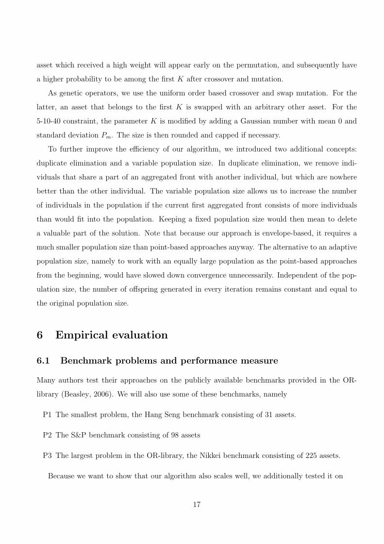
The results on all 4 benchmark problems are summarized in Tables 1 to 4. Table 1 reports on

the max-delta-area, i.e. the area between obtained efficient frontier and ideal front with wide

margins, for the cardinality constrained problem at the end of the run. The same information,

but with respect to ideal-delta-area, is provided in Table 2. As can be seen, E-MOEA significantly

outperforms P-MOEA on all benchmark problems. In terms of the ideal-delta-area, the relative

performance of P-MOEA is somewhat better, indicating that it particularly has a problem in

finding the portfolios with high expected return or low variance.

The results for the problem with 5-10-40 constraint look similar (see Tables 3 and 4), although

the differences between P-MOEA and E-MOEA are generally smaller.

Typically obtained efficient frontiers for P1 and P3 with cardinality constraint are depicted in

19

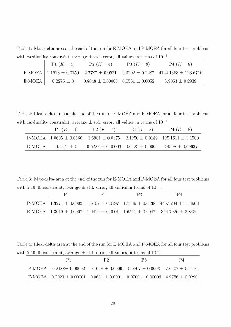
Table 1: Max-delta-area at the end of the run for E-MOEA and P-MOEA for all four test problems

with cardinality constraint, average ± std. error, all values in terms of 10−6.

P1 (K = 4) P2 (K = 4) P3 (K = 8) P4 (K = 8)

P-MOEA 1.1613 ± 0.0159 2.7787 ± 0.0521 9.3292 ± 0.2287 4124.1363 ± 123.6716

E-MOEA 0.2275 ± 0 0.8048 ± 0.00003 0.0561 ± 0.0052 5.9063 ± 0.2939

Table 2: Ideal-delta-area at the end of the run for E-MOEA and P-MOEA for all four test problems

with cardinality constraint, average ± std. error, all values in terms of 10−6.

P1 (K = 4) P2 (K = 4) P3 (K = 8) P4 (K = 8)

P-MOEA 1.0605 ± 0.0160 1.6981 ± 0.0175 2.1250 ± 0.0189 125.1611 ± 1.1580

E-MOEA 0.1371 ± 0 0.5222 ± 0.00003 0.0123 ± 0.0003 2.4398 ± 0.09637

Table 3: Max-delta-area at the end of the run for E-MOEA and P-MOEA for all four test problems

with 5-10-40 constraint, average ± std. error, all values in terms of 10−6.

P1 P2 P3 P4

P-MOEA 1.3274 ± 0.0002 1.5107 ± 0.0197 1.7339 ± 0.0138 446.7284 ± 11.4963

E-MOEA 1.3019 ± 0.0007 1.2416 ± 0.0001 1.6511 ± 0.0047 344.7926 ± 3.8489

Table 4: Ideal-delta-area at the end of the run for E-MOEA and P-MOEA for all four test problems

with 5-10-40 constraint, average ± std. error, all values in terms of 10−6.

P1 P2 P3 P4

P-MOEA 0.2188± 0.00002 0.1028 ± 0.0009 0.0807 ± 0.0003 7.6607 ± 0.1116

E-MOEA 0.2023 ± 0.00001 0.0631 ± 0.0001 0.0700 ± 0.00006 4.9756 ± 0.0290

20

0.0008

0.001

0.0012

0.0014

0.0016

0.0018

0.004 0.005 0.006 0.007 0.008

varia

nce

expected return

P-MOEAE-MOEA

ideal front

0.0002

0.0004

0.0006

0.0008

0.001

0.0012

0.0014

0.0016

0.0018

0 0.001 0.002 0.003 0.004

varia

nce

expected return

P-MOEAE-MOEA

ideal front

Figure 4: Typical fronts obtained on test problem P1 (left) and test problem P3 (right) with

cardinality constraint.

Figure 4. As can be seen, for the small problem (P1), both algorithms perform quite well. In fact,

the figure zooms in on only a part on the front, as on a plot of the whole front, the differences

would be hard to see. Still, E-MOEA clearly outperforms P-MOEA and is indistinguishable from

the ideal front over large parts. For the larger problem, P-MOEA does not seem to be able to

come close to the performance of E-MOEA. In particular in the area of higher returns, there are

clear deficiencies. It seems that P-MOEA does not scale very well to larger problem sizes6. One

reason may be that there are usually only few assets with a high return, and exactly those have to

be combined in the portfolio to obtain an overall high return. Identifying the high-return assets

out of a large set may prove difficult for the P-MOEA. E-MOEA on the other hand finds solutions

hardly distinguishable from the ideal front also for the larger problems.

For the 5-10-40 constraint, the fronts obtained by P-MOEA and E-MOEA are much closer

to each other, and further away from the ideal front. Still, the front obtained by E-MOEA

dominates P-MOEA’s front basically everywhere. Note that again for visibility, the plot for the

larger problem only shows a segment of the overall front.

When looking at the obtained solution quality in terms of max-delta-area over running time,

it is clear that the advantage of E-MOEA over P-MOEA is significant throughout the run. Fig-

ure 6(a) looks at P3 with cardinality constraint. Clearly, E-MOEA starts out much better, and

converges much faster than P-MOEA (for the small problem, E-MOEA even found the best so-

6In Streichert et al. (2004a,b, 2003), the algorithm was only tested on small problems with up to 81 assets.

21

0.0007

0.0008

0.0009

0.001

0.0011

0.0012

0.0013

0.003 0.004 0.005 0.006

varia

nce

expected return

P-MOEAE-MOEA

ideal front

0.00036

0.00038

0.0004

0.00042

0.00044

0.00046

0.00048

0.0005

0.0016 0.0018 0.002 0.0022 0.0024

varia

nce

expected return

P-MOEAE-MOEA

ideal front

Figure 5: Typical fronts obtained on test problem P1 (left) and test problem P3 (right) with

5-10-40 constraint.

lution within 5 out of the allowed 250 seconds in every single run). Note that we plot against

running time. Because E-MOEA has to run a critical line algorithm for every individual, it can

only evaluate about 13500 individuals during the 1000 seconds allowed, while P-MOEA generates

and evaluates approx. 1,945,000 individuals in the same time frame.

For the problem P3 with 5-10-40 constraint, E-MOEA also starts better than P-MOEA, then

P-MOEA quickly catches up only to fall behind again (see Figure 6(b)). The difference in the

number of individuals evaluated is even more striking here than for P3 with cardinality constraint,

because the 5-10-40 constraint does not allow to remove a large fraction of the assets for the

critical line algorithm. While E-MOEA can generate only about 3000 individuals in the given

2000 seconds, P-MOEA generates approx. 3,475,000.

One explanation for the superiority of E-MOEA, besides being envelope-based, is certainly

its in-built weight optimization by the critical line algorithm. This effect is visible in Figure 7,

which compares the solution quality or randomly generated solutions with both, the P-MOEA and

the E-MOEA. Clearly, E-MOEA has a much better start, as the majority of randomly generated

envelopes is clearly better than the majority of randomly generated portfolios.

22

0

2e-06

4e-06

6e-06

8e-06

1e-05

1.2e-05

1.4e-05

1.6e-05

0 100 200 300 400 500 600

max

. del

ta-a

rea

time

P-MOEAE-MOEA

1.6e-06

1.8e-06

2e-06

2.2e-06

2.4e-06

0 200 400 600 800 1000

max

. del

ta-a

rea

time

P-MOEAE-MOEA

Figure 6: Convergence curves for P3 with cardinality constraint (left) and 5-10-40 constraint

(right).

0.0007

0.0008

0.0009

0.001

0.0011

0.0012

0.0013

0.0014

0.0015

0.0016

0.002 0.0025 0.003 0.0035 0.004 0.0045 0.005 0.0055 0.006

V(w

)

E(w)

ideal front500 random envelopes

200,000 random portfolios

Figure 7: Randomly initialized populations of envelopes and portfolios for the 5-10-40 problem

and the Hang Seng Dataset.

23

7 Conclusion

The critical line algorithm is a very efficient algorithm to calculate the whole efficient frontier for a

standard mean-variance portfolio selection problem. However, this method is no longer applicable

if practical real-world constraints such as maximum cardinality constraint, buy-in thresholds, or

the 5-10-40 rule from the German investment law have to be considered, because such constraints

render the search space non-convex. Researchers have therefore resorted to solving these problems

point-based, approximating the efficient frontier by iteratively solving a sub-problem with a fixed

expected return, for many different settings of the expected return. Because even the sub-problems

are rather complex, often meta-heuristics are used.

In this paper, we have proposed a new envelope-based multi-objective evolutionary algorithm

(E-MOEA), which is a combination of a multi-objective algorithm with an embedded algorithm

for parametric quadratic programming. The task of the MOEA is to define a set of convex subsets

of the search space. Then, for each subsets the critical line algorithm can efficiently generate an

efficient frontier which we call envelope. The combination of all generated envelopes then forms

the overall solution to the problem.

To our knowledge, our approach is the first metaheuristic approach which is not point-based,

but which is capable of generating a continuous front of alternatives for portfolio selection problems

with non-convex constraints. Compared with a state-of-the-art point-based MOEA, E-MOEA was

shown to find significantly better frontiers in a shorter time.

As future work, we are planning to integrate a more intelligent mutation operator that uses

shadow prices to influence mutation probabilities. Also, the ideas of envelope-based MOEAs

should be transferred to other applications. In particular, we are planning to consider portfolio

re-balancing problems that include consideration of fixed and variable transaction costs.

Acknowledgements: We would like to thank Ralph Steuer for providing us the large bench-

mark test cases.

References

Armananzas, R. and Lozano, J. A. (2005). A multiobjective approach to the portfolio optimization problem. In

Congress on Evolutionary Computation, pages 1388–1395. IEEE.

24

Beasley, J. E. (2006). Or-library. online, http://people.brunel.ac.uk/∼mastjjb/jeb/info.html.

Best, M. J. and Kale, J. K. (2000). Quadratic Programming for Large-Scale Portfolio Optimization. In Keyes, J.,

editor, Financial Services Information Systems, pages 513–529. CRC Press LLC.

Bienstock, D. (1996). Computational study of a family of mixed-integer quadratic programming problems. Math-

ematical Programming, 74(2):121–140.

Chang, T.-J., Meade, N., Beasley, J. B., and Sharaiha, Y. (2000). Heuristics for cardinality constrained portfolio

optimisation. Computers & Operations Research, 27:1271–1302.

Coello, C. C., Veldhuizen, D. A. V., and Lamont, G. B. (2002). Evolutionary Algorithms for solving multi-objective

problems. Kluwer.

Crama, Y. and Schyns, M. (2003). Simulated annealing for complex portfolio selection problems. European Journal

of Operational Research, 150(3):546–571.

Deb, K. (2001). Multi-Objective Optimization using Evolutionary Algorithms. Wiley.

Derigs, U. and Nickel, N.-H. (2001). On a metaheuristic-based DSS for portfolio optimization and managing

investment guideleines. In Metaheuristics International Conference.

Derigs, U. and Nickel, N.-H. (2003). Meta-heuristic based decision support for portfolio optimization with a case

study on tracking error minimization in passive portfolio management. OR Spectrum, 25:345–378.

Eddelbuttel, D. (1996). A hybrid genetic algorithm for passive management. Computing in economics and finance,

Society of Computational Economics.

Ehrgott, M., Klamroth, K., and Schwehm, C. (2004). An MCDM approach to portfolio optimization. European

Journal of Operational Research, 155:752–770.

Eiben, A. E. and Smith, J. E. (2003). Introduction to evolutionary computing. Springer.

Elton, E., Gruber, M., Brown, S., and Goetzmann, W. (2003). Modern Portfolio Theory and Investment Analysis.

John Wiley and Sons, 6th edition.

Fieldsend, J. E., Matatko, J., and Peng, M. (2004). Cardinality constrained portfolio optimisation. In Yang, Z. R.,

Everson, R. M., and Yin, H., editors, Intelligent Data Engineering and Automated Learning, volume 3177 of

LNCS, pages 788–793. Springer.

Hirschberger, M., Qi, Y., and E., S. R. (forthcoming). Randomly generating portfolio-selection covariance matrices

with specified distributional characteristics. European Journal of Operational Research.

25

Huang, C.-f. and Litzenberger, R. H. (1988). Foundations for Financial Economics. Elsevier Science Publishing

Co., Inc.

InvG (2004). Investmentgesetz (InvG). online: http://www.bafin.de/gesetze/invg.htm.

Jobst, N. J., Horniman, M. D., Lucas, C. A., and Mitra, G. (2001). Computational aspects of alternative portfolio

selection models in the presence of discrete asset choice constraints. Quantitative Finance, 1:489–501.

Lin, D. and Wang, S. (2002). A genetic algorithm for portfolio selection problems. Advanced Modeling and

Optimization, 4(1):13–27.

Maringer, D. and Kellerer, H. (2003). Optimization of cardinality constrained portfolios with a hybrid local search

algorithm. OR Spectrum, 25:481–495.

Maringer, D. G. (2002). Werpapierselektion mittels Ant Systems. Zeitschrift fur Betriebswirtschaft, 72(12):1221–

1240.

Markowitz, H. M. (1952). Portfolio selection. Journal of Finance, 7:77–91.

Markowitz, H. M. (1956). The Optimization of a Quadratic Function Subject to Linear Constraints. Naval Research

Logistics Quarterly, 3:111–133.

Markowitz, H. M. (1987). Mean-Variance Analysis in Portfolio Choice and Capital Markets. Blackwell Publishers.

Miettinen, K. (1998). Nonlinear multiobjective optimization. Kluwer.

NEOS Guide (2006). Optimization software guide. online:

http://www-fp.mcs.anl.gov/otc/Guide/SoftwareGuide/.

Schaerf, A. (2002). Local search techniques for constrained portfolio selection problems. Computational Economics,

20(3):170–190.

Scheckenbach, B. (2006). Envelope-based portfolio optimization with complex constraints. Master’s thesis, Institute

AIFB, University of Karlsruhe, Germany.

Schlottmann, F. and Seese, D. (2004). Financial applications of multi-objective evolutionary algorithms: recent

development and future research directions. In Coello-Coello, C. and Lamont, G., editors, Applications of

Multi-Objective Evolutionary Algorithms, pages 627 – 652. World Scientific.

Schlottmann, F. and Seese, D. (2005). A hybrid heuristic approach to discrete multi-objective optimization of

credit portfolios. Computational Statistics Data Analysis, 47(2):373 – 399.

Stein, M., Branke, J., and Schmeck, H. (2006). Efficient implementation of an active set algorithm for large scale

portfolio selection. Technical report, Institute AIFB, University of Karlsruhe.

26

Streichert, F., Ulmer, H., and Zell, A. (2003). Evolutionary algorithms and the cardinality constrained portfolio

optimization problem. In GOR Operations Research Conference, pages 253–260. Springer.

Streichert, F., Ulmer, H., and Zell, A. (2004a). Comparing discrete and continuous genotypes on the constrained

portfolio selection problem. In Genetic and Evolutionary Computation Conference, volume 3103 of LNCS, pages

1239–1250.

Streichert, F., Ulmer, H., and Zell, A. (2004b). Evaluating a hybrid encoding and three crossover operators on the

constrained portfolio selection problem. In Congress on Evolutionary Computation, volume 1, pages 932–939.

IEEE Press.

Zitzler, E., Thiele, L., Laumanns, M., Fonseca, C. M., and da Fonseca, V. G. (2003). Performance assessment of

multiobjective optimizers: An analysis and review. IEEE Transactions on Evolutionary Computation, 7(2):117–

132.

27