Embed Size (px)
Citation preview

1
Yongqiang Cui, Shuai Zhai
Professor Marcel Blais
Math 574
12/1/16
Portfolio Optimization Project Report
Abstract
In this project, we close the portfolio established in the Portfolio Optimization Project. A
complete analysis of our portfolio including the construction, week-to-week performance,
week-to-week rebalancing process and overall performance will be given in this report. Ratio
analysis, Leverage analysis and basic risk measure are conducted by analyzing the portfolio
returns in time series. At the end of the project, a good-of-fit hypothesis test was performed to
determine the returns distribution’s consistence with our fitted distributions.
Introduction
The portfolio that we used to analyze is generated from Markowitz optimal portfolio from the
Portfolio Optimization Project. On 11/09/2016, The portfolio was constructed with calculated
weight of twenty stocks. The weight of different stocks was rebalanced each week until
12/06/2016, the date on which portfolio was closed. The total return of holding this portfolio
in this month is $22,923, with the initial capital of $500,000. Our portfolio value is increased
by 4.58% in the holding period. We choose S&P 500 as the market portfolio which grows
from 2,163.26 to 2,212.23 in the last month, with an increase of 2.25%. Thus, the overall
performance of our portfolio is good as it has a higher growth rate than our chosen market
portfolio.
Methodology
Our portfolio is formed based on the Modern portfolio theory, or mean-variance analysis,
introduced by Harry Markowitz in 1952. It is a mathematical framework for assembling a
portfolio of assets to maximize the expected return for a given level of risk, defined as
variance. (Markowitz, 1952)
Historical stock price of last one year was used to in our project to estimate the weights in
Markowitz optimal portfolio. We first use our data of stock price to calculate the optimal
portfolio with different expected return and variance, code listed in appendix (1). Then
combine the optimal portfolios to create an efficient frontier, code in appendix (2). Tangency
line with the intercept of risk-free rate of the efficient frontier, which is called the tangency
portfolio could be found using code appendix (3). After that, construct the Markowitz optimal
portfolio with the weights of tangency portfolio. In each of the following week, we will add
the stocks’ price of the new week into historical data and rebalance the weight of stocks in
the portfolio. The market value of stocks and the portfolio was recorded for analyzing
purpose.
2
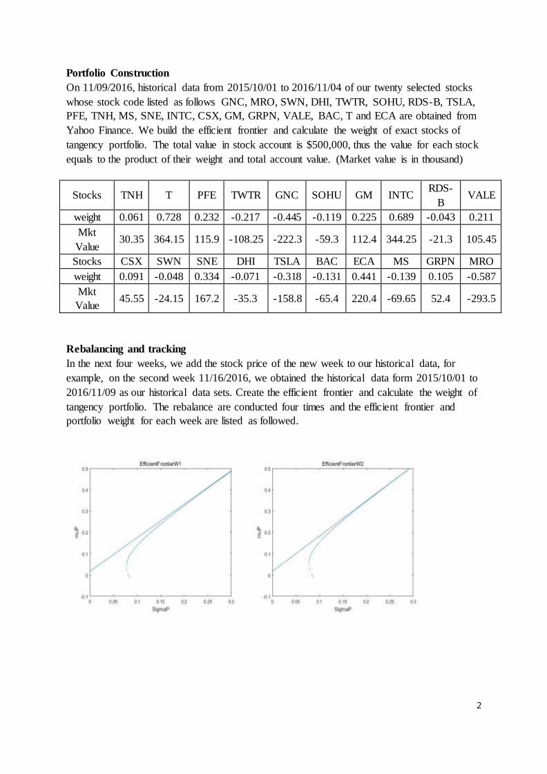
Portfolio Construction
On 11/09/2016, historical data from 2015/10/01 to 2016/11/04 of our twenty selected stocks
whose stock code listed as follows GNC, MRO, SWN, DHI, TWTR, SOHU, RDS-B, TSLA,
PFE, TNH, MS, SNE, INTC, CSX, GM, GRPN, VALE, BAC, T and ECA are obtained from
Yahoo Finance. We build the efficient frontier and calculate the weight of exact stocks of
tangency portfolio. The total value in stock account is $500,000, thus the value for each stock
equals to the product of their weight and total account value. (Market value is in thousand)
Stocks TNH T PFE TWTR GNC SOHU GM INTC RDS-
B VALE
weight 0.061 0.728 0.232 -0.217 -0.445 -0.119 0.225 0.689 -0.043 0.211
Mkt
Value 30.35 364.15 115.9 -108.25 -222.3 -59.3 112.4 344.25 -21.3 105.45
Stocks CSX SWN SNE DHI TSLA BAC ECA MS GRPN MRO
weight 0.091 -0.048 0.334 -0.071 -0.318 -0.131 0.441 -0.139 0.105 -0.587
Mkt
Value 45.55 -24.15 167.2 -35.3 -158.8 -65.4 220.4 -69.65 52.4 -293.5
Rebalancing and tracking
In the next four weeks, we add the stock price of the new week to our historical data, for
example, on the second week 11/16/2016, we obtained the historical data form 2015/10/01 to
2016/11/09 as our historical data sets. Create the efficient frontier and calculate the weight of
tangency portfolio. The rebalance are conducted four times and the efficient frontier and
portfolio weight for each week are listed as followed.

3
Date 11/9/2016 11/16/2016 11/23/2016 12/1/2016
Min up 0.0396 0.0511 0.051 0.0621
Min Variance 0.006 0.0061 0.0061 0.0061
From the comparison of efficient frontier, minimum variances are almost constant and its
corresponded portfolio returns increase in the last four weeks.
And the corresponding tangency portfolio weights are listed as followed:
2016/11/9 2016/11/16 2016/11/23 2016/11/30 Average
MRO -0.5870 -0.2965 -0.2843 -0.2231 -0.3477
GNC -0.4446 -0.3018 -0.2898 -0.2085 -0.3112
TWTR -0.2165 -0.1697 -0.1540 -0.1434 -0.1709
BAC -0.1308 0.2814 0.4481 0.5072 0.2765
SWN -0.0483 -0.1852 -0.1832 -0.1313 -0.1370
MS -0.1393 -0.0334 0.0847 -0.0648 -0.0382
SOHU -0.1186 -0.2562 -0.2887 -0.2137 -0.2193
DHI -0.0706 -0.4836 -0.3367 -0.2988 -0.2974
TSLA -0.3176 -0.3158 -0.3518 -0.2278 -0.3033
RDS B -0.0426 -0.1951 -0.2877 -0.2620 -0.1969
TNH 0.0607 0.1067 0.0758 0.0757 0.0797
CSX 0.0911 0.3590 0.2184 0.1932 0.2154
PFE 0.2318 0.2207 -0.0162 -0.0225 0.1035
GM 0.2248 0.4276 0.2434 0.2199 0.2789
SNE 0.3344 0.2072 0.1198 0.0357 0.1743
T 0.7283 0.8825 1.2254 1.1876 1.0060
INTC 0.6885 0.1652 0.1812 0.0938 0.2822
GRPN 0.1048 0.0602 0.0398 0.0330 0.0595
VALE 0.2109 0.1697 0.1457 0.1451 0.1679
ECA 0.4408 0.3570 0.4100 0.3045 0.3781

4
We attempted to keep the data period of exact one year by delating a week’s data at the
beginning and adding one week’s date at present. However, the results run by our Markowitz
Optimal Model do not make us satisfied. The weight of portfolio for a new week changes too
much too rebalance on Interactive Brokers. Thus, we choose to update new weeks’ stock
price and extend the period of our historical stock price. The returns covariance matrix does
not change a lot.
Portfolio Performance
From the total value of Interactive Brokers Accounts which consists of $504,128 cash and
$499,823 Stock in the first week. The total account value ends up in $1,026,814, the invest
return of holding this portfolio for one month is $22,923. Our portfolio value is increased by
2.28% within the holding period. Compared to our chosen market portfolio S&P 500 which
grows from 2,163.26 to 2,212.23 in the last month, with an increase of 2.25%. The overall
performance of our portfolio is good as it has a higher rate of return.
Ratio Analysis:
We use the S&P 500 as benchmark and in our models, we use sample mean return estimate
p , use sample standard deviation of returns to estimate volatility and use the 10-year Treasury
Yield as our risk-free rate f :

5
Date Portfolio Return Market Return
Excess Return(up-
um)
Excess Return(up-
uf)
2016/12/6 0.001000514 0.003410879435 -0.002410365435 0.000921929058
2016/12/5 0.010795234 0.005821300668 0.004973933332 0.01071664906
2016/12/2 0.001143647 0.0003970644614 0.0007465825386 0.001065062058
2016/12/1 -0.038764015 -0.00351553795 -0.03524847705 -0.03884259994
2016/11/30 -0.005836422 -0.002653470376 -0.003182951624 -0.005915006942
2016/11/29 0.029008915 0.001335319659 0.02767359534 0.02893033006
2016/11/28 0.016074101 -0.005254478505 0.02132857951 0.01599551606
2016/11/25 0.021870169 0.003914329257 0.01795583974 0.02179158406
2016/11/23 -0.007135212 0.0008080111124 -0.007943223112 -0.007213796942
2016/11/22 0.02008148 0.002165427763 0.01791605224 0.02000289506
2016/11/21 0.007069175 0.007461386865 -0.0003922118647 0.006990590058
2016/11/18 0.007708739 -0.002386700318 0.01009543932 0.007630154058
2016/11/17 0.003950144 0.004676288736 -0.0007261447356 0.003871559058
2016/11/16 0.039926843 -0.001582285738 0.04150912874 0.03984825806
2016/11/15 -0.00288217 0.007480824323 -0.01036299432 -0.002960754942
2016/11/14 -0.030046657
-
0.0001155027836 -0.02993115422 -0.03012524194
2016/11/11 -0.035896756 -0.001397936775 -0.03449881923 -0.03597534094
2016/11/10 -0.011609604 0.001950759502 -0.0135603635 -0.01168818894
Mean 0.001469895833 0.001250871074 0.0002190247591 0.001391310891
Standard
Dev 0.02128609889 0.003713625597 0.020881997 0.02128609889
The plots of the portfolio returns are showed as followed:
Then we use the following measures to analyze our portfolio:
-0.06
-0.04
-0.02
0
0.02
0.04
0.06
11/1
0/20
16
11/1
1/20
16
11/1
2/20
16
11/1
3/20
16
11/1
4/20
16
11/1
5/20
16
11/1
6/20
16
11/1
7/20
16
11/1
8/20
16
11/1
9/20
16
11/2
0/20
16
11/2
1/20
16
11/2
2/20
16
11/2
3/20
16
11/2
4/20
16
11/2
5/20
16
11/2
6/20
16
11/2
7/20
16
11/2
8/20
16
11/2
9/20
16
11/3
0/20
16
12
/1/2
01
6
12
/2/2
01
6
12
/3/2
01
6
12
/4/2
01
6
12
/5/2
01
6
12
/6/2
01
6
Daily Return

6
(1) Sharpe Ratio: p f
p
RS
(2) Treynor Ratio: p f
p
RT
,
2
PMp
M
(3) Information Ratio p f
Rp RM
RI
(4) Sortino Ratio:
Definition:The dispersion of X from a given value a is
2 2( ) ( )a x a f x dx
.
In finance, we are concerned about downside dispersion from some value a i.e. X taking
values in ( , ]a define the semi variance of X about a is
2 2( ) ( )a x a f x dx
.
Given sample R1, R2, R3…Rn of returns with some distribution f(x), Define ,
,
i
i
i i
a R ay
R R a
,
then the downside sample semi variance is
2 2 2
1 1
1 1( ) [min(0, )]n n
a i i i iS y a R an n
So, we use
f
p f
S
to estimate the Sortiono Ratio
0
0p
r
r
.
Outcomes:
Sharp Ratio Treynor Ratio Information Ratio Sortino Ratio
0.06390022971 0.001292279398 0.008901856247 0.09195970697
The Sortino Ratio is a modification of the Sharpe Ratio but penalizes only those returns falling
below our expected return, while the Sharpe ratio penalizes both upside and downside volatility
equally. The difference between the Sharpe ratio and the Information Ratio is that the
Information Ratio aims to measure the risk-adjusted return in relation to a benchmark. A
variation of the Sharpe ratio is the Sortino ratio, which removes the effects of upward price
movements on standard deviation to measure only return against downward price volatility and
uses the semi variance in the denominator. The Treynor ratio uses systematic risk, or beta (β)
instead of standard deviation as the risk measure in the denominator.

7
Comparing through these ratios, it shows that all the ratios are all positive indicating that our
portfolio perform well. However, these values of ratios are not very high, Treynor Ratio and
Information Ratio are even around zero. We could conclude that although our portfolio could
make money, we still take additional risks.
(5) Maximum drawdown:
The maximum drawdown (MDD) up to time T is,
(0, ) (0, )( ) max[max ( ) ( )]
T tMDD T X t X
Peak value valley value Maximum drawdown Maximum drawdown/Peak Value
992236 925201 67035 6.76%
During this period, huge loss was suffered in our portfolio with a maximum drawdown of 6.76%
within four trading days.
(6) Portfolio alpha and beta
It is based on Jensen performance measure,
( )p p f p m f
Portfolio Beta 0.03333847659
Portfolio Alpha 0.0001460887197
With a positive Alpha 0.0001460887197, it means although our portfolio performs better than
the benchmark, its value is around 0 which means our portfolio’s performance is very close
to the market performance. And the Beta is 0.03, indicating that our portfolio return has
potential risk in some way.
(7) Comparison of our portfolio performance to industry benchmarks
As far as we are concerned, by comparing to the benchmarks, the overall performance of our
portfolio is very close to the benchmarks’. But we take additional risks comparing to the market.
850000900000950000
100000010500001100000
11/1
0/20
16
11/1
1/20
16
11/1
2/20
16
11/1
3/20
16
11/1
4/20
16
11/1
5/20
16
11/1
6/20
16
11/1
7/20
16
11/1
8/20
16
11/1
9/20
16
11/2
0/20
16
11/2
1/20
16
11/2
2/20
16
11/2
3/20
16
11/2
4/20
16
11/2
5/20
16
11/2
6/20
16
11/2
7/20
16
11/2
8/20
16
11/2
9/20
16
11/3
0/20
16
12/1
/201
6
12/2
/201
6
12/3
/201
6
12/4
/201
6
12/5
/201
6
12/6
/201
6
Market value

8
(8) While trading on Interactive Brokers, we are limited by the Margin calls. The portfolio
weight calculated by Markowitz Optimal Model sometimes cannot be exercised because you
need to short too much stocks. The margin calls will appear for some unreasonable weight of
portfolio. We adjust our portfolio by changing one or several stocks and calculate the weight
for new portfolio. Usually, we delate the stocks which requires to do more short position from
the Model. Repeat this process until we found an exercisable weight of tangency portfolio.
Leverage Analysis
Date Total Debt
Leverage
Ratio
2016/12/6 2336947.85 2.33694785
2016/12/5 2314261.48 2.31426148
2016/12/2 2287899.17 2.28789917
2016/12/1 2303301.716 2.303301716
2016/11/30 2696540.848 2.696540848
2016/11/29 2654664.216 2.654664216
2016/11/28 2673747.689 2.673747689
2016/11/25 2703091.755 2.703091755
2016/11/23 2691175.457 2.691175457
2016/11/22 2826370.712 2.826370712
2016/11/21 2795538.602 2.795538602
2016/11/18 2748163.639 2.748163639
2016/11/17 2747769.797 2.747769797
2016/11/16 2732490.91 2.73249091
2016/11/15 2574427.828 2.574427828
2016/11/14 2538839.014 2.538839014
2016/11/11 2534622.348 2.534622348
2016/11/10 2531621.124 2.531621124
2016/11/9 2516046.038 2.516046038
The leverage ratio of our portfolio stays around 2.5, which is the highest level that avoid the
margin calls. A higher leverage ratio will cause margin calls and we need to adjust the portfolio
0
1
2
3
11/9/20…
11/11/2…
11/13/2…
11/15/2…
11/17/2…
11/19/2…
11/21/2…
11/23/2…
11/25/2…
11/27/2…
11/29/2…
12/1/20…
12/3/20…
12/5/20…
Leve
rage
Rat
io
Date
Leverage Ratio vs. Date
Leverage Ratio

9
composition by changing several stocks.
Capstone Part
Basic risk Measure
In this part, we use volatility of returns, Value-at-risk (VaR) and Conditional value-at- risk
(CVaR) as the weekly risk measures of our portfolio. For VaR and CVaR, we use the parametric
method to estimate them with both a normal and a student-t returns distribution and three
different confidence level (1%, 5%, 10%).
Method introduction:
Gaussian VaR and CVaR
Let 2-x /21
2e
(x)= denote the PDF of the standard normal distribution, and let (x)
denote the corresponding CDF with ' . The Gaussian quantile function ( )Q is the
function satisfying the condition
( ( ))Q
for all : 0 1 .
In the case of a Gaussian distribution with mean and variance 2 , the quantile function
of that distribution is then ( )Q and the corresponding “Value at Risk”, or VaR, is just
the negative of the quantile, which is
( ) ( )VaR Q
The CVaR is a related entity, giving the average in a tail bounded by the corresponding VaR
level. In general, for a density function ( )f x linked to a random variable X, we would need to
know
( )1[ | ( )] ( )
Q
E X X Q xf x dx
In the case, because ' x , so that for a standard normal distribution
1[ | ( )] ( ( ))E X X Q Q
and applying a scaling and translation to get the general case gives us, for the loss
( ) ( ( ))CVaR Q
In the case of a Gaussian system, there is no substantive diff erence between the VaR and CVaR

10
measures: both take the form
( ) ( )Risk
where ( ) ( )Q in the case of VaR and 1
( ) ( ( ))Qu
in the case of CVaR.
Student’s T VaR and CVaR
The pdf of the Student’s T distribution is
2 ( 1)/2
1 [( 1) / 2] 1( , )
[ / 2] (1 / ) v
vh t v
v t vv
It is like the pdf function in Gaussian case. Define the quantile function ( , )TQ n for a standard
univariate T distribution (n is the degree of freedom). If we wish to parametrize the problem
again by mean and standard deviation, the VaR will be given by
2( ) ( , )T
nVaR Q n
n
The relevant function for this case is not the (negative of the) standard T quantile but the
negative of the scaled unit variance T quantile
2( ) ( , ) ( , )T
nQ n Q n
n
:
The VaR measure of risk is now in standard form ( ) .
For the CVaR, we need to find the integral of ( , )nh n and we can find the function
1
/2 2 2 21
( )( )2( , )
2 ( )2
v vv v t
k t vv
Then the CVaR with mean and variance 2 is now
2 1( ) ( , )T
nCVaR k Q n
n
( ),
and now the 2 1
( ) ( , )T
nk Q n
n
( ),
By calculation by MATLAB, we get the four weeks’ VaR and CVaR. (William, 2011)

11
Volatility analysis:
We compare the volatility of our portfolio returns with the market volatility, which in our case
is the volatility of the S&P500 index.
Week1 Week2 Week3 Week4
Portfolio Return Volatility 2.99% 0.97% 2.75% 0.56%
Market Volatility 0.37% 0.37% 0.38% 0.27%
By comparing across weeks, the Week4 has the smallest volatility (0.56%), and the Week2 also
has a smaller volatility (0. 97%).The volatilities of week1 and week3 are near 3%. As the result,
the Week2 and Week4 shows the lower risk of all four weeks. So, our portfolio has a relevantly
high volatility to the market performance. And comparing to the market performance, our
portfolio has a relevantly high volatility to the market volatility. Our portfolio shows higher
risk than it should have. (Wagner, 2007)
VaR analysis:
We sort the four weeks VaR data and plot them.
The degree of freedom of T distribution is 3 according to the MATLAB function mle ().
VaR(Gaussian) VaR(T)
Confidence level 1% 5% 10% Confidence level 1% 5% 10%
Week1 0.0777 0.0573 0.0464 Week1 0.086 0.0547 0.0422
Week2 0.0165 0.0098 0.0063 Week2 0.0192 0.009 0.0049
Week3 0.0595 0.0408 0.0308 Week3 0.0672 0.0385 0.054
Week4 0.0087 0.0049 0.0029 Week4 0.0104 0.0033 9.85E-04
2.99%
0.97%
2.75%
0.56%
0.00%
0.50%
1.00%
1.50%
2.00%
2.50%
3.00%
3.50%
Week1 Week2 Week3 Week4
Volalitility

12
To explain the VaR clearly, we choose the VaR(Gaussian) with the confidence level 5% of the
Week1 as an example, 0.0573 means that there is a 0.05 probability that the portfolio return
will fall by more than 0.0573 this week. It can also be said that with 95% confidence that the
worst daily loss will not exceed 0.0573. So for the same confidence leve, the high VaR means
the higher potential risk that the porfolio has.
By comparing the tables and plots, with the same confidence and distribution, the VaR of
Week2 and Week4 is always very small. With the 5% and 10% confidence level of T
distributuion, we find that the returns of Week2 and Week4 still show lower risks.
CVaR analysis:
The CVaR is the second name of Expected Shortfall (ES). For example, with 5% level, the
"expected shortfall at 5% level" is the expected return on the portfolio in the worst 5% of cases.
So, with the same confidence level, the higher the CVaR, the lower the risk of the portfolio has.
For the tendency of the CVaR is same for the different confidence level. We choose the case
with 5% confidence level to analyze. (Carlo & Dirk, 2002).
5% confidence level CVaR(Gaussian) CVaR(T)
Week1 -0.98 -1.02
Week2 -0.33 -0.55
Week3 -0.91 -0.94
Week4 -0.19 -0.37
0.0777
0.0165
0.0595
0.0087
0.0573
0.0098
0.0408
0.0049
0.0464
0.0063
0.0308
0.0029
0
0.02
0.04
0.06
0.08
0.1
0.12
0.14
0.16
0.18
0.2
Week1 Week2 Week3 Week4
VaR(Gaussian)
1% 5% 10%
0.086
0.0192
0.0672
0.0104
0.0547
0.009
0.0385
0.0033
0.0422
0.0049
0.054
9.85E-04
0
0.02
0.04
0.06
0.08
0.1
0.12
0.14
0.16
0.18
0.2
Week1 Week2 Week3 Week4
VaR(T)
1% 5% 10%

13
`
By comparing the table and plots with two distributions, the Week2 and Week4 suffer from the
lower expected loss. Meanwhile, the Week1 and Week3 have higher risks.
Goodness-of fit Hypothesis
Form a time series of daily returns from our factor modeling project. Here we choose the
French and Fama model include F1 (Short-Term Reversal Factor). Time series of daily
returns and the bate values of this model are both obtained from factor modeling project.
French&F1 beta0 Mkt-RF SMB HML ST_Rev E(R)
VALE 0.000314 0.014083 -0.004220 0.009180 0.018838 -0.002803
ECA 0.001019 0.012178 0.013284 0.026709 0.018977 -0.003691
GRPN 0.000135 0.008741 0.007860 -0.003348 0.007406 -0.004060
MRO 0.000738 0.014722 0.008103 0.021085 0.012380 -0.003185
SWN 0.000840 0.009314 0.010014 0.020318 0.021306 -0.005241
BAC 0.000176 0.013188 0.001662 0.007796 -0.002979 0.000468
TWTR 0.000152 0.008076 0.011793 -0.005722 0.007450 -0.002960
TSLA -0.000204 0.010725 -0.002283 -0.008123 0.002006 0.001080
MS 0.000205 0.015092 0.003453 0.007975 -0.003709 -0.000358
CSX 0.000105 0.011817 0.000131 0.003794 0.001772 -0.001069
DHI 0.000070 0.012115 0.004077 0.000071 -0.000445 0.000955
TNH 0.000180 0.004035 0.001439 0.004614 0.005232 -0.001230
-1.20
-1.00
-0.80
-0.60
-0.40
-0.20
0.00
Week1 Week2 Week3 Week4
CVaR
CVaR(Gaussian) CVaR(T)

14
T 0.000012 0.007878 -0.001435 0.002348 -0.001589 0.000227
INTC -0.000029 0.009575 -0.002245 0.000318 0.000403 0.000390
GM 0.000012 0.010057 -0.002267 0.001510 0.001890 -0.000126
GNC 0.000317 0.010536 0.015396 0.001217 0.001803 -0.001497
PFE -0.000110 0.008961 -0.000972 -0.004850 0.001589 -0.000093
SNE -0.000046 0.011447 -0.002676 -0.001292 0.003126 -0.000470
RDS-B 0.000327 0.009771 0.001995 0.010535 0.005610 -0.001448
SOHU 0.000160 0.006784 0.003418 -0.000794 0.012175 0.000764
Fit our returns distribution to both normal and a t density distribution. For normal distribution,
we calculate the mean, standard deviation and the z value to create the plot. For Student T
distribution, degree of freedom is required to be considered. We calculated it using MATLAB
function mle () which turns out to be 8.3174.
0123456789
-2.8
2828
0613
-2.6
239
-2.4
195
-2.2
152
-2.0
108
-1.8
064
-1.6
020
-1.3
977
-1.1
933
-0.9
889
-0.7
846
-0.5
802
-0.3
758
-0.1
714
0.03
29
0.2
373
0.4
417
0.6
460
0.85
04
1.05
48
1.2
592
1.4
635
1.6
679
1.87
23
2.07
66
2.2
810
2.4
854
2.6
898
2.89
41
3.09
85
3.30
29
PDF&Histogram of Normal Dist
0123456789
-2.8
2828
0613
-2.6
239
-2.4
195
-2.2
152
-2.0
108
-1.8
064
-1.6
020
-1.3
977
-1.1
933
-0.9
889
-0.7
846
-0.5
802
-0.3
758
-0.1
714
0.03
29
0.23
73
0.44
17
0.64
60
0.85
04
1.05
48
1.25
92
1.46
35
1.66
79
1.87
23
2.07
66
2.28
10
2.48
54
2.68
98
2.89
41
3.09
85
3.30
29
CDF&Histogram of Student's T Dist

15
Then use the time series of daily returns to perform a goodness- of-fit hypothesis test. Assign
data to 60 intervals in a histogram and acquire the frequency for each interval. Then denote Pi
as the probability of normal distribution with Cumulative Distribution Function F, calculate Pi
for each interval i using formula. (Jensen, 1968)
1
t
( ) ( ) ( )i i i
i hIn erval
P f y dy F y F y
iN Pg =theoretical frequency.
Chi-square test statistic:
22
1
( )n i i
ii
u N P
N P
g
g
Use the same formula to calculate the 2 value for Student-t distribution
0
2
4
6
8
10
12
14
-0.0
270
-0.0
243
-0.0
216
-0.0
189
-0.0
162
-0.0
135
-0.0
108
-0.0
081
-0.0
054
-0.0
027
0.00
00
0.00
27
0.00
54
0.00
82
0.01
09
0.01
36
0.01
63
0.01
90
0.02
17
0.02
44
0.02
71
Histogram of Original Data
Frequency
0
0.2
0.4
0.6
0.8
1
1.2
-0.03 -0.02 -0.01 0 0.01 0.02 0.03 0.04
CDF
Normal Student-T
16
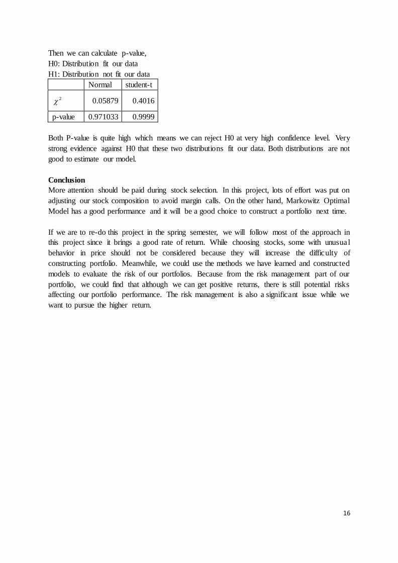
Then we can calculate p-value,
H0: Distribution fit our data
H1: Distribution not fit our data
Normal student-t
2 0.05879 0.4016
p-value 0.971033 0.9999
Both P-value is quite high which means we can reject H0 at very high confidence level. Very
strong evidence against H0 that these two distributions fit our data. Both distributions are not
good to estimate our model.
Conclusion
More attention should be paid during stock selection. In this project, lots of effort was put on
adjusting our stock composition to avoid margin calls. On the other hand, Markowitz Optimal
Model has a good performance and it will be a good choice to construct a portfolio next time.
If we are to re-do this project in the spring semester, we will follow most of the approach in
this project since it brings a good rate of return. While choosing stocks, some with unusua l
behavior in price should not be considered because they will increase the difficulty of
constructing portfolio. Meanwhile, we could use the methods we have learned and constructed
models to evaluate the risk of our portfolios. Because from the risk management part of our
portfolio, we could find that although we can get positive returns, there is still potential risks
affecting our portfolio performance. The risk management is also a significant issue while we
want to pursue the higher return.

17
Appendix:
m-files
1.
(1).
function [ optimalWeights ] = optimalPortfolio( expReturns, CovMatrix, expPortfolioReturn)
mu = expReturns ;
Omega = CovMatrix;
N=length(mu);
muP=expPortfolioReturn;
One = ones(length(mu),1) ;
invOmega = inv(Omega) ;
A = One'*invOmega*mu ;
B = mu'*invOmega*mu ;
C = One'*invOmega*One ;
D = B*C - A^2 ;
h=invOmega*(C*mu/D-A*One/D);
g=invOmega*(B*One/D-A*mu/D);
optimalWeights =h*muP+g;
end
(2).
N=length(expPortfolioReturn);
for i=1:N
[ optimalWeights] = optimalPortfolio( expReturns, CovMatrix, expPortfolioReturn(i));
SigmaStar(i)=sqrt(optimalWeights'*CovMatrix*optimalWeights);
end
plot(SigmaStar,expPortfolioReturn)
title('efficientFrontier')
xlabel('SigmaP')
ylabel('muP')
(3). function [ TangencyWeights ] = TangencyPortfolio( expReturns, CovMatrix,muf)
mu = expReturns ;
Omega = CovMatrix;
N=length(mu);
One = ones(length(mu),1) ;
invOmega = inv(Omega) ;
A = One'*invOmega*mu ;
B = mu'*invOmega*mu ;
C = One'*invOmega*One ;
D = B*C - A^2 ;
h=invOmega*(C*mu/D-A*One/D);
g=invOmega*(B*One/D-A*mu/D);

18
w=invOmega*(mu-muf*One);
TangencyWeights=w/(One'*w);
end
2.
function [ Sharp,Treynor,Sortino,Alpha,Beta ] = Ratios( Rp, Rm,uf)
n=length(Rp);
uRp=mean(Rp);
StDRp=std(Rp);
uRm=mean(Rm);
StDRm=std(Rm);
ExcessRpm=Rp-Rm;
uExcessRpm=mean(ExcessRpm);
StDexcess=std(ExcessRpm);
Sharp=(uRp-uf)/StDRp;
A=cov(Rp,Rm);
B=A(1,2)/var(Rm);
for i=1:n
Rpf(i)=Rp(i)-uf;
end
meanRpf=mean(Rpf);
Treynor =meanRpf/B;
Information=ExcessRpm/StDexcess;
Beta=A(1,2)/var(ExcessRpm);
Alpha=uExcessRpm-uf+Beta*(uRm-uf);
for i=1:n
if (Rp(i)-uf)<0
negative(i)=Rp(i)-uf;
end
end
Downside=(sumsqr(negative)/n)^0.5;
Sortino=meanRpf/Downside;
end
2.
function [VaRnormal,CVaRnormal,VaRt,CVaRt,CVaRTt] = ValueAtRisk(returns,alpha,v)
n=length(returns);
m=mean(returns);
sigma=std(returns);
S=sqrt(sigma^2*n/(n-1));
x=norminv([alpha 1-alpha],0,1);

19
t=tinv(alpha,v);
C=x(1);
VaRnormal=-m-sigma*C;
CVaRnormal=-m+sigma*C/alpha;
VaRt=-m-sigma*sqrt((v-2)/v)*t;
CVaRTt=(-((v^(-1/2)*(v+t^2)))/(alpha*beta(v/2,1/2)*(n-1)))*((1+t^2/n)^(-(v+1/2)));
end
Reference
1. Markowitz, H. (1952). Portfolio Selection. The Journal of Finance, 7(1), 77.
doi :10.2307/2975974
2. Wagner, H. (2007). Volatility's Impact On Market Returns. Retrieved December 12, 2016,
from http://www.investopedia.com/articles/financial-theory/08/volatility.asp
3. Carlo Acerbi; Dirk Tasche (2002). "Expected Shortfall: a natural coherent alternative to
Value at Risk" (pdf). Economic Notes. 31: 379–388. doi:10.1111/1468-0300.00091
4. William T. S. (2011). Risk, VaR, CVaR and their associated Portfolio Optimizations when
Asset Returns have a Multivariate Student T Distribution;
5. Jensen, M.C. (1968), “The Performance of Mutual Funds in the Period 1945-1964,”
Journal of Finance 23, 1968, pp. 389-416.