Portfolio Allocation over Life-Cycle with Multiple Late-in-Life

Saving Motives

Minjoon Lee∗

November 22, 2015

Job Market Paper

Link to the latest version

Abstract

Older households face health-related risks, including risk of being in need of long-term care and

mortality risk. Portfolio choice depends on the interaction between these health-related risks and

household preferences for long-term care and bequests. Using linked survey-administrative data

on clients of a mutual fund company, this paper finds that the desire to have enough resources

for long-term care and bequests are overall strong but also heterogeneous across households.

The estimated relationship between actual stock share of households and the strength of these

preferences is qualitatively similar but quantitatively much weaker compared to the predictions

from the life-cycle model with the estimated preference heterogeneity. Based on the predictions

from the model, this paper discusses what financial instruments would better meet the needs of

households.

∗University of Michigan (e-mail: minjoon@umich.edu). This research is supported by a program project grant fromthe National Institute of Aging P01-AG026571. The Vanguard Group Inc. supported the data collection through theVRI (Vanguard Research Initiative). Vanguards Client Insight Group and IPSOS SA were responsible for implementingthe VRI survey and provided substantial input into its design. John Ameriks, Andrew Caplin, and Matthew Shapiroare co-principal investigators of the VRI. I gratefully acknowledge their role in this project and advice on this research.The design of the VRI benefited from the collaboration and assistance of Joseph Briggs, Wandi Bruine de Bruin, AlyciaChin, Mi Luo, Brooke Helppie McFall, Ann Rodgers, and Christopher Tonetti as part of the program project, fromAnnette Bonner (Vanguard), and Wendy O’Connell (IPSOS SA). I am grateful to Stefan Nagel and John Laitner forcomments on earlier draft. I gratefully acknowledge financial support from the Korea Foundation for Advanced Studiesduring my Ph.D. For documentation of the VRI, including a dynamic link to the survey instrument, see http://ebp-projects.isr.umich.edu/VRI/.

1 Introduction

Older households face multiple risks in retirement. Most importantly, they face health-related risks,

including considerable expenditure risk associated with long-term care (LTC) and mortality risk.

Given the high cost of LTC, the risk of being in need of LTC effectively increases households’ risk

aversion, limiting their ability to take additional risks in the financial market for a higher expected

return. Mortality risk adds another layer of uncertainty that may further reduce room for risky assets

in households’ financial portfolio. In household portfolio choice literature, relatively little attention has

been given to the implications of these health-related background risks on portfolio choice, in particular

on the choice of the share of risky assets. Instead, most research on household portfolio choice has

focused on the effects of labor income uncertainty (see Benzoni, Collin-Dufresne, and Goldstein, 2007;

Bodie, Merton, and Samuelson, 1992; Cocco, Gomes, and Maenhout, 2005; and Viceira, 2001, among

others), which is not a major source of background risk for households that are near or in retirement.

This study addresses this gap in the literature by examining how these health-related background

risks affect portfolio allocation over the life-cycle.

Health-related risks have complex effects on decisionmaking of households because they likely affect

preferences directly. Hence, how they affect asset accumulation, portfolio choices, and spending will

depend on preferences about related expenditures. For example, for households who have a preference

for high-quality, expensive service when they need LTC, the same probability of being in need of LTC

implies effectively a much larger expenditure risk. Similarly, two households with equal mortality risk

may choose different portfolios depending on the strength of the bequest motive. Moreover, the paper

will show that there are complicated and subtle interactions of preferences over LTC and bequests

with health-related risks.

This paper uses distinctive modeling approach and measurement infrastructure to study the

financial decisionmaking of households facing these late-in-life risks. The approach uses novel survey

instruments to identify preferences relevant to late-in-life portfolio choices. It uses survey responses

to quantify the distribution of these preferences in the population and then to relate these preferences

to choices and outcomes in a new dataset—the Vanguard Research Initiative (VRI)—that combines

survey and administrative account information on a large population of older Americans who have

sufficient financial assets to make these portfolio choices highly relevant.

Specifically, I first estimate households’ preferences for expenditures in the LTC state and bequests

using responses to hypothetical survey questions. Estimated utility functions for LTC expenditures

1

and bequests not only show the strength of the precautionary saving motive for LTC and the bequest

motive over the life-cycle, but also govern households’ exposure to health-related background risks

for a given amount of resources. I then investigate the empirical relationship between the estimated

strength of these two saving motives and actual stock share of households to see whether households’

actual portfolio choice responds to health-related background risks. I also study how the optimal

stock share should respond to the strength of these saving motives using a life-cycle portfolio choice

model with the estimated preference heterogeneity. Lastly, I contrast the findings from the empirical

and theoretical analyses to derive implications for a better design of financial advice and financial

products.

I begin by finding empirical evidence that the preferences for LTC expenditures and bequests are

both strong but also heterogeneous among households. For many households, the estimated preference

parameters suggest that their life-cycle saving is mainly driven by a precautionary motive associated

with LTC or a bequest motive. On the other hand, a non-trivial fraction of households appear to

put much larger weight on their consumption in the state of good health than LTC expenditures or

bequests.

My analysis using the life-cycle model with the estimated preference heterogeneity suggests that

both a stronger preference for LTC expenditures and a stronger bequest motive imply lower optimal

stock share. The more households care about expenditures in the LTC state, the more painful a

combination of a negative stock return shock and an LTC shock is. The impact of the LTC preference is

limited for households with fewer resources, because for them publicly-funded nursing home functions

as a partial insurance against negative stock return shocks. The mechanism behind the effect of the

bequest motive is subtler. On one hand, most households consider bequest as a luxury good, which

effectively makes households who put more weight on bequests than consumption less risk averse.

On the other hand, the existence of retirement income and LTC risk under the presence of mortality

risk makes households with a stronger bequest motive more reluctant to take risks in the financial

market, compared to households who mainly care about own consumption. I show that the latter

effect dominates the former in my calibrated model, so a stronger bequest motive lowers the optimal

stock share.

I find that the relationship between observed actual household portfolio choice and estimated

preferences is qualitatively similar but quantitatively weaker than suggested by the life-cycle model.

To be specific, a stronger preference for LTC expenditure is associated with lower stock share, though

2

the size of the estimated effect is overall much smaller than the predictions from the model. I

do not find a significant relationship between the preference for bequests and actual stock share.

The discrepancy between the empirical results and the theoretical results might indicate that what

households actually do is different from what they should do, which, in turn, suggests a necessity for

better design of financial instruments (Campbell, 2006). Using simulated life-cycle profiles from the

model solutions, I show that financial instruments need to incorporate implications of the estimated

preference heterogeneity not only in determining the initial level of stock market exposure but also in

the adjustment of stock share over the life-cycle.

The structure of the rest of the paper is as follows. Section 2 discusses the related literature.

Section 3 describes the VRI. In Section 4, I explain my methodology of structural preference parameter

estimation and present the estimation results. The empirical relationship between household stock

share and the preference parameters is discussed in Section 5. In Section 6, I derive the theoretical

effects of preference heterogeneity on portfolio choices using a life-cycle model. I discuss the

implications of the gap between empirical and theoretical findings in Section 7.

2 Literature

The preference parameter estimation in this paper is based on the methodology of Barsky, Juster,

Kimball, and Shapiro (1997, hereafter BJKS) and Kimball, Sahm, and Shapiro (2008, hereafter KSS).

They estimate the distribution of risk preference parameter using survey responses and allowing

for survey response errors. KSS also construct individual cardinal proxies for the risk preference

parameters using the estimates from the structural model, which can be used as a right-hand side

variable in a linear regression without concerns about an attenuation bias. This paper extends their

methodology to the case with multiple preference parameters.

This paper is also related to the literature on the estimation of health-state-dependent and

bequest utility functions. De Nardi, French, and Jones (2010), Ameriks, Caplin, Laufer, and van

Nieuwerburgh (2011), Lockwood (2014) and Ameriks, Briggs, Caplin, Shapiro, and Tonetti (2015a)

estimate preference parameters for a health-state-dependent utility function and/or bequest utility

function by either using a structural model only or combining a structural model with SSQs, but they

do not allow for heterogeneity in these preferences. Ameriks, Briggs, Caplin, Shapiro, and Tonetti

(2015b) estimate heterogeneity in risk preference, precautionary saving motive for LTC, and bequest

3

motive using the SSQs from the VRI. This study differs from theirs in that I examine the impact

of preferences on portfolio allocations, while they examine the impact of preferences on demand

for LTC insurance as well as annuities. In addition, I estimate the population distribution of the

preference parameters following the method outlined in KSS, while Ameriks, Briggs, Caplin, Shapiro,

and Tonetti (2015b) estimate their parameters at the individual level. In Appendix D, I provide a

detailed comparison of the two estimation methodologies. Finally, my study addresses Finkelstein,

Luttmer, and Notowidigdo’s (2009) conclusion that using the observed demand for assets with state-

dependent returns is the most promising approach in estimating health-state-dependent utility. The

SSQs allow us to use this approach in this study.

This paper also adds to the literature that empirically analyzes the effects of health-related

risks and bequest motives on households stock share by distinguishing the role played by preference

heterogeneity from that due to other channels. There is a large body of research, including Rosen and

Wu (2004), Berkowitz and Qiu (2006), Fan and Zhao (2009), Love and Smith (2010), and Goldman

and Maestas (2013), that studies how actual changes in health status (or expected health-related

expenditures) affect the stock holdings of households. The literature suggests either no effect or a

small negative effect. There is not as much work on the effect of bequest motives on stock share.

Hurd (2002) finds no evidence that intended bequests have an effect on stock share, while Spaenjers

and Spira (2014) find that households with children tend to have a higher stock share. In most

of these empirical studies, the main explanatory variables are remote proxies for (expected) health

expenditures and bequests. The remote nature of these proxies makes it challenging to identify the

channel behind any observed effect. This paper clearly identifies the effects of preference heterogeneity,

controlling for other channels such as effects of different economic and demographic conditions, using

responses to the SSQs.

Finally, this paper contributes to the theoretical life-cycle portfolio choice literature by

investigating the implications of heterogeneous saving motives. Bodie, Merton, and Samuelson

(1992), Viceira (2001), Cocco, Gomes, and Maenhout (2005) and Benzoni, Collin-Dufresne, and

Goldstein (2007) use a life-cycle portfolio choice model to analyze the effect of labor income on

the optimal stock share. In these papers, retirement is simply considered to be a period without

background risk. By contrast, my study provides a more precise understanding of older households

by examining how health-expenditure and mortality risk impact portfolio choices. Ding, Kingston,

and Purcal (2014) investigate the effect of a bequest motive on the optimal stock share in the absence

4

of health expenditure shocks and income flow. Pang and Warshawsky (2010) and Reichling and

Smetters (2015) study annuity demand using a life-cycle model with exogenous health expenditure

risk and bequest motives. This paper solves for the optimal stock share under a life-cycle model that

features realistically-calibrated processes for health and income, options for LTC service, and, most

importantly, preference heterogeneity estimated from the VRI data.

3 Data

The paper uses the Vanguard Research Initiative (VRI) to estimate the distribution of the structural

preference parameters as well as the empirical relationship between households stock share and

heterogeneous preferences for LTC expenditures and bequests. The VRI is a linked survey-

administrative dataset on more than 9,000 Vanguard account holders who are at least 55 years old.

The VRI is an Internet survey. There have been three surveys to date on different subject areas. The

administrative account data provides both the sample frame and monthly account balance data.

This dataset is appropriate for the research question of this paper for several reasons. First,

it contains ample observations of wealthholders, for whom LTC precautionary saving motives and

bequest motives are operative. Second, the Strategic Survey Question responses from the VRI survey

allow us to estimate preference parameters. Finally, it includes comprehensive and accurate measures

of wealth and stock shares for the account holders. In the following, I discuss each of these features

in greater detail.1

3.1 Sample Composition: Ample Observations of Wealthholders

By design, the VRI collects data on households with non-negligible wealth that are facing key financial

decisions in retirement such as annuitization, the purchase of long-term care insurance, or portfolio

allocation choices. In contrast, the Health and Retirement Study (HRS), the leading representative

survey of older Americans, has a large fraction of households with not enough financial wealth to face

such decisions (Poterba, Venti, and Wise, 2011).

The goal of obtaining ample observations of wealthholders is achieved as the VRI is roughly

representative of top 50 percent of households in the wealth distribution. The sampling screen that

is used to target wealthholders—the requirement that they have at least $10,000 in their Vanguard

1See Ameriks, Caplin, Lee, Shapiro, and Tonetti (2014) for complete description.

5

accounts—made the VRI sample wealthier by its construction than the more representative samples,

such as the HRS and Survey of Consumer Finances (SCF). Ameriks, Caplin, Lee, Shapiro, and Tonetti

(2014) show that the VRI is broadly representative of the top half of the wealth distribution and with

the similar sampling screens HRS and SCF respondents have similar characteristics as the VRI. In

addition, about half of the VRI sample between the ages of 55 and 64 is composed of those who have

only employer-sponsored accounts at Vanguard. For this group the selection would be less an issue,

and Ameriks, Caplin, Lee, Shapiro, and Tonetti (2014) actually show that their characteristics are

even closer to those of the comparable subsets of the HRS and SCF.

3.2 Strategic Survey Questions

In its second survey (conducted in winter 2014), the VRI implemented Strategic Survey Questions

(SSQs) to elicit information regarding preferences about risk, expenditures on LTC, and bequests. In

the following I briefly introduce aspects of the SSQs that are relevant for this paper (see Ameriks,

Briggs, Caplin, Shapiro, and Tonetti, 2015b for a thorough description of these SSQs).

SSQs put respondents in hypothetical situations so that cross-sectional differences in responses

can be interpreted as signals of preference heterogeneity. Under hypothetical situations that are not

related to their actual financial situations and demographics (including age and health conditions),

respondents are asked to choose between hypothetical financial products.

This paper uses three types of SSQs:

• A gamble on consumption to elicit risk preference (SSQ1)

• A trade-off between expenditures in a state of good health versus those in the LTC state, to

elicit state-dependent preference for LTC (SSQ2)

• A trade-off between expenditures in the LTC state and bequests to measure the strength of the

bequest motive (SSQ3)

The responses to SSQs can be used to identify the preference parameters in the three utility

functions, one for expenditures in the healthy state, one for expenditures in the LTC state, and one

6

for bequests. To do so, I use the fully parametric functional forms:

U(X) =(X + κ)1−1/γ

1− 1/γ

ULTC(X) = θLTC(X + κLTC)1−1/γ

1− 1/γ

UBeq(X) = θBeq(X + κBeq)

1−1/γ

1− 1/γ,

(1)

where the X is expenditure in each health state, i.e., good health, LTC state, and bequest/death. γ

is risk tolerance parameter, θ is a utility multiplier governing the strengths of the precautionary LTC

saving and bequest motives, and κ is a necessity parameter for each utility function, determining

whether the expenditures are considered necessities or luxuries (κ being negative means the

expenditures are necessaries, while it being positive means they are luxuries). The functional form

for the LTC state and bequest utility functions are the same as those in Ameriks, Briggs, Caplin,

Shapiro, and Tonetti (2015a, 2015b). For reasons that will be clear, this paper includes a necessity

parameter κ in the healthy state utility function to explain the increase in risk aversion with lower

resources found in SSQ1.

In the following, I describe key aspects of setups of each SSQ and distribution of responses. (Table

A1 in Appendix A shows the exact setups and wording for each SSQ.) I will also discuss which moment

of the SSQ response distributions mainly identifies each preference parameter. I defer more detailed

explanation on the modeling of preference heterogeneity, the modeling of survey response errors and

the preference parameter estimation procedure to Section 4.

In SSQ1, the key elements of the hypothetical situation are as following. Respondents are at age

80; they live alone and rent their home; it is assumed that they will be healthy for the following

year. Respondents have to choose between Plan A and Plan B, where Plan A guarantees a fixed level

of consumption ($W ) while Plan B has a 50 percent chance of doubling it ($2W ) and a 50 percent

chance of reducing it by x percent ($(1− 0.01x)W ) for the following year. Since the question is asked

for a sequence of values of x where the sequence depends on the respondent’s previous responses, it

provides a risk range ([xmin, xmax]) which encapsulates the respondents indifference point.2

Figure 1(a) shows two noticeable patterns in the distribution of responses to the SSQ1. The vast

majority of respondents are not willing to take more than 33 percent of risk to have a chance to

2The setup of SSQ1 draws on the hypothetical question used in BJKS and KSS, with a difference that the questionused in their papers is about a gamble on income not consumption.

7

double their consumption, implying they are overall quite risk intolerant. In addition, when the same

question is asked with a relatively lower initial consumption level ($50,000 instead of $100,000), the

results show that respondents tend to be more risk averse. This phenomenon is inconsistent with a

homothetic utility function under which we should observe the same response distribution regardless

of initial consumption level, motivating the necessity parameter in the healthy-state utility function.

In terms of mapping to the preference parameters in the healthy-state utility function, the overall

level of risk a respondent is willing to take in SSQ1 identifies γ while how much she become more risk

averse with a lower initial consumption level identifies κ.

In SSQ2, it is assumed that respondents will need a LTC service with probability π in the coming

year. There is no publicly-funded LTC service and no one can take care of the respondent for free.

They have to allocate the given resources ($W ) between Plan C and Plan D, where Plan C pays the

respondent $(1/π) for every $1 of investment only if the respondent needs an LTC service and Plan

D pays $1 for every $1 of investment only if the respondent is healthy in the coming year. In the LTC

state, respondents need to finance both their LTC expenditures and their other consumption needs

out of returns from Plan C. Responses to SSQ2 are measured as the amount of money they choose to

invest in Plan C.

Figure 1(b) shows that, in SSQ2, the median respondent allocates resources in such a way that

they secure more resources in the LTC state than in the healthy state. For example, when respondents

are given W = $100, 000 with an LTC probability of π = 1/4 , to have the same amount of resources

across two states, they should invest $20,000 in Plan C. That is indeed close to one of two modal

allocations in the distribution, but the majority of respondents invest more than that. This implies

level of θLTC greater than one. How much the share allocated to Plan C changes across different

values of W and π identifies κLTC .

Lastly, in SSQ3, respondents are assumed to be in the last year of their lives and in need of an

LTC service for the entire year. Again there is no publicly-funded LTC service and no informal care.

Respondents need to allocate the given resources ($W ) between Plan E and Plan F, where money in

Plan E will be used to finance their own needs while that in Plan F will be bequeathed. Responses

to SSQ3 are measured as the amount of money they choose to put in Plan E.

Figure 1(c) shows that, in SSQ3, when the given resources (W ) is $100,000, many respondents

choose not to leave a bequest, but the number of respondents choosing to leave a bequest increases

as W increases. This suggests that bequests may be perceived as luxury goods rather than necessary

8

expenditures (hence κBeq is positive). Among those who leave bequests, many leave sizeable bequests,

implying that once the bequest motive becomes active (i.e., once they have enough resources) it tends

to be strong (hence θBeq is greater than one).

The SSQs have the following common features for eliciting preferences. Each type of SSQ is asked

multiple times with different amounts of given initial resources ($W ) and/or with the likelihood of

relevant events (π). In addition to identifying preference parameters as just discussed, this test-retest

feature enables us to separately identify the distribution of survey response errors. The SSQ scenarios

are also stationary questions embedded in a life-cycle setting. Except for SSQ3 (where it is assumed

that respondents die at the end of the following year), it is assumed that the same situation repeats

at the end of the following year. Respondents do not have any other resources than what is given

in the assumed situations; they are not allowed to either borrow from future or save for future. By

shutting down borrowing and lending, responses to SSQs can be interpreted as solutions of single-

period maximization problems.3

The VRI survey takes a number of steps to make the SSQ scenarios more understandable. In the

administration of the survey, respondents are provided with the scenario-specific rules prior to making

their decisions. They are also allowed to refer back to the rules via a hover button at any point in the

decision process. The survey also tests understanding of scenarios before asking SSQs. A majority of

respondents were able to give correct answers to more than 80 percent of the verification questions.

Since the survey is conducted on the Internet, it takes advantage of the ability to visualize the

trade-offs of the SSQs. In SSQ2 and SSQ3, participants are asked to make their choices using a novel

slider interface (see Figure A1 in Appendix A). This interface dynamically informs participants of the

resources they will have in each state as a result of the current allocation.4

3.3 Wealth and Stock Share Measurement

The wealth and stock share measures are from the first survey of the VRI (conducted in fall 2013).

The measures cover the entire financial portfolio and housing wealth of the households.

The wealth and stock share measures of the VRI are based on a comprehensive account-by-account

3Note that with constant amount of resources, the life-cycle solution will not involve much borrowing or lendingunless the interest rate is different from time discount rate, so the assumption of no borrowing and lending is notdrastically counterfactual.

4See Ameriks, Briggs, Caplin, Shapiro, and Tonetti (2015b) for more detail about verification of rule understanding,the slider interface, and the other mechanisms used for the SSQs. They also show that the SSQ responses are coherentboth internally (i.e., there is a strong positive correlation among answers within each SSQ type) and externally (i.e.,characteristics that might affect relevant preferences do have predictive power on responses).

9

approach. Respondents are asked about the types of accounts they have (e.g., IRAs, savings, mutual

funds), the number of accounts of each type, and the balance and stock share of each account. This

account-by-account format matches the way respondents keep track of their own wealth and does not

require them to sum balances across accounts to provide total figures for asset categories that are

familiar to economists but not necessarily to survey respondents.

The accuracy of the wealth and stock measures is validated by comparing them to the Vanguard

administrative account records for those accounts they indicate are held at Vanguard. The comparison

shows that the survey measure of wealth is very accurate: the median percentage difference between

the survey and administrative measures of total assets held at Vanguard is essentially zero while the

length of the interquartile range is only several percentage points.5

This paper uses the stock share of households’ entire financial portfolio measured from the survey

as the main dependent variable in the empirical analysis.

3.4 Characteristics of the Sample

In addition to the SSQ responses and wealth measures, I use information on household demographics

as well as subjective probability measures regarding their longevity and future need for a LTC service.

Table 1 presents the distribution of the variables used in this study beyond the SSQs.

Almost everyone in the VRI is a stock holder, which is not surprising given that the sample

is composed of Vanguard clients. Therefore, the identification of any effect on stock holding comes

through the intensive margin rather than through the extensive margin, so the interpretation of results

of this paper is free from participation cost issues (see Vissing-Jorgensen, 2002). The demographic

composition of the VRI sample is as follows. About two-thirds are coupled and two-thirds are male.

By design, the VRI respondents are evenly distributed across the following age bins: [55, 59], [60,

64], · · · , and 75+. Furthermore, again by design, about half of those below age 65 are from the

employer-sponsored sample. Most 401(k) participants roll over to an IRA when they retire, so there

are few employer-sponsored accounts for those aged over 65. As a result, about 20 percent of the

entire sample are from the employer-sponsored sample. In terms of health, the vast majority of the

sample report that their health is better than or equal to good (using a five-point scale excellent, very

good, good, fair, and poor). About 40 percent have a post college degree while another 33 percent

have a college degree. Finally, the median (mean) household annual income and financial wealth are

5See Ameriks, Caplin, Lee, Shapiro, and Tonetti (2014) for more details on the wealth measurement in the VRI.

10

$83,443 ($126,132) and $723,665 ($1,101,468).

As another measure of heterogeneity in household health, the VRI survey asks each participant to

estimate her probability of needing at least one year of LTC service as well as her prediction of how

likely it is that she will reach a certain age. The results for the VRI sample show that 45 percent

expect to require at least one year of LTC service, with remarkable heterogeneity across responses

(the interquartile range is [15%, 75%]). The subjective probability questions about reaching certain

ages are asked for a set of ages determined as ({75, 85, 95} ∩ {t|t ≥ current age + 5}). The median

response for the lowest age asked (the measure used in this study) is 85 percent.

Finally, to control for the heterogeneous exposure to LTC expenditure risk caused by LTC

insurance, I include the indicator variable of having LTC insurance. Twenty-three percent of the

respondents have a LTC insurance policy.

4 Estimation of Structural Preference Parameters

In this section I estimate distributions of the structural preference parameters that govern the

preferences for LTC expenditures and bequests, based on the methodology of Barsky, Juster, Kimball,

and Shapiro (1997, hereafter BJKS) and Kimball, Sahm, and Shapiro (2008, hereafter KSS). The

estimates obtained in this section are used to construct the regressors in the empirical analysis in

Section 5 and to calibrate the life-cycle model in Section 6.

4.1 Methodology

I extend the methodology of BJKS and KSS to estimate joint distribution of multiple preference

parameters. I model the respective strengths of the preference for LTC expenditure and that for

bequests using a utility multiplier and a necessity parameter for the utility function representing each

motivation. Using MLE, I jointly estimate the distributions of these parameters as well as that of

the risk preference parameter. Having multiple observations for each type of SSQ enables us also to

identify the distribution of the survey response errors.6 Cardinal proxies for the preference parameters

are calculated as the conditional expectations using the estimated distributions. In the following, I

explain each element of the estimation methodology in detail.

6To be more specific, to identify distributions of N parameters in addition to survey response errors, we need at leastN + 1 observed responses per individual. In other words, the distribution of SSQ responses should have at least onemore degree of freedom than can be explained solely by the distributions of the true preference parameters, to allowroom for survey response errors.

11

Utility functions As I previewed in Section 3, I assume three utility functions, one for expenditures

in the healthy state, one for expenditures in the LTC state, and one for bequests:

Ui(X) =(X + κ)1−1/γi

1− 1/γi

ULTC,i(X) = θLTC,i(X + κLTC,i)

1−1/γi

1− 1/γi

UBeq,i(X) = θBeq,i(X + κBeq,i)

1−1/γi

1− 1/γi,

(2)

where subscript i denotes each individual.

The necessity parameter (κ) in the healthy-state utility function has important implications for

portfolio choice. Merton (1971) shows that, in a continuous-time model with stock return risk (modeled

as an i.i.d. process) as the only uncertainty, for a household with the utility function I assume for the

state of good health, the optimal stock share is determined as:

π =µsσ2η

γ(1 +(Y + κ)(1− er(t−T ))

rW), (3)

where µs is the risk premium, ση is the standard deviation of the stock return, Y is the income

flow without uncertainty, t is the current time, T is the end of the investment horizon, and W is

current wealth. The role of κ is obtained through the ratio between income plus κ and wealth (Y+κW ).

Intuitively, we expect that a higher income-to-wealth ratio should imply a higher optimal stock share,

as the present value of the income flow (human capital) becomes a close substitute for a risk-free asset

in the absence of income uncertainty.7 According to (2), what is compared to wealth is not the gross

level of income but rather the income net of the subsistence level of consumption (negative of κ).8

Identification Here I briefly review which moment of the SSQ response distribution mainly

identifies each preference parameter.9 The risk tolerance parameter (γ) is mainly identified by the

7This intuition holds even with income uncertainty as long as income shocks are not highly correlated with stockreturn shocks (Viceira, 2001; Cocco, Gomes, and Maenhout, 2005).

8It should be noted that a negative κ (−κ) can also be interpreted as (slow-moving) habit in consumption.Habit formation has been used to explain macroeconomic phenomena such as a high risk premium (Campbell andCochrane, 1999). Both Gomes and Michaelides (2003) and Polkovnichenko (2007) examine the effect of habit formationon household portfolio choices, while Brunnermeier and Nagel (2008) test the microeconomic implications of habitformation. Although I do not explicitly model (the negative of) κ as a time-varying habit, this study provides empiricalevidence for this necessity parameter. In a related paper, Wachter and Yogo (2010) explain why more affluent householdshave a higher stock share using a two-good—basic and luxury—model, where households are less risk averse over luxurygood consumption. κ can be considered to be a reduced form representation of this two-good model, since both modelsgenerate lower risk aversion for households with larger wealth.

9The full relationship between survey responses and preference parameters is complex and non-linear, in particularunder the presence of survey response errors. Later in this section, I provide detailed explanations regarding how I

12

level of risk that respondents are willing to take in SSQ1. The necessity parameter in the healthy state

utility function (κ) is identified by the effect of the initial resource level on the responses in SSQ1. It

should be noted that since SSQ1 consists of only two questions, we cannot estimate the distributions

of both γ and κ and identify survey response errors at the same time. Therefore, I assume that there

is heterogeneity only in γ (hence no subscript i for κ in (2)).10 The utility multipliers for LTC state

expenditure (θLTC) and bequest (θBeq) are mainly identified by the average share of resources that

respondents allocate for LTC expenditures and bequests in SSQ2 and SSQ3. The necessity parameters

for those two utility functions (κLTC , κBeq) are mainly identified by how the level of given resources

affects responses in SSQ2 and SSQ3.

Modeling heterogeneity in preference parameters Following KSS, I model the cross-person

heterogeneity of preference parameter as draws from probability distributions. I assume the

distribution of the risk tolerance parameter and those of the utility multipliers on LTC expenditure and

bequest to be log-normal, while those of the necessity parameters for LTC expenditure and bequest

to be normal:

log(γi) ∼ N(µγ , σ2γ) (4)

log(θLTC,i) ∼ N(µLTC , σ2LTC) (5)

log(θBeq,i) ∼ N(µBeq, σ2Beq) (6)

κLTC,i ∼ N(µκ,LTC , σ2κ,LTC) (7)

κBeq,i ∼ N(µκ,Beq, σ2κ,Beq). (8)

Log-normality assumption prevents the risk preference parameter and utility multipliers from being

negative. These functional form assumptions are also consistent with shape of survey responses

distributions shown in Figure 1. I also assume that the preference parameters are statistically

independent, except for potential dependence through observed covariates.11

model preference heterogeneity and the survey response process.10When I estimate the distributions of the parameters conditional on the covariates used in the stock share regression,

I assume that κ is homogenous conditional on the covariates (i.e., κ is a deterministic function of these covariates). Themotivation for estimating the distributions conditional on the covariates is explained in Section 5.

11As will be explained below, in one version of estimation I model the mean (µ) parameter of each of these distributionsas a linear function of all the covariates used in the stock share regression. Hence I do allow for correlations betweenpreference parameters through these covariates.

13

Modeling of survey response errors I model the survey responses as the sum of the solutions

of the underlying optimization problems for the SSQs and “trembling-hand” type survey response

errors, where “trembling-hand” means that error terms are added to the survey responses (instead of

preference parameters or utilities). Given the realizations of the preference parameters from (4)-(8),

we can determine the solutions of the optimization problems underlying the SSQs. I assume that

survey response errors are independent across questions and normally distributed with a mean of

zero:

εi,kj ∼ N(0, σε,kj), (9)

where kj denotes the jth question of SSQ type k.

In the following, I show how to map the SSQ responses to the solutions of the corresponding

optimization problems under the presence of the survey response errors.

1) SSQ1: Let W1j be the amount of consumption given in the jth question in SSQ1. Given γi and κ,

the level of risk (in terms of the percentage loss associated with the risky gamble) at which individual

i becomes indifferent between the risky gamble and the guaranteed consumption can be determined

as x∗i,1j ,12 such that:

(W1j + κ)1−1/γi

1− 1/γi= 0.5

(2W1j + κ)1−1/γi

1− 1/γi+ 0.5

((1− x∗i,1j)W1j + κ)1−1/γi

1− 1/γi. (10)

The indifference point that is actually used in answering the survey question, xi,1j , is determined as:

xi,1j = x∗i,1j + εi,1j . (11)

This determines the risk range within which the observed response falls.

2) SSQ2: The underlying optimization problem for the jth question of SSQ2 is:

Maxx (1− π2j)(W2j − xi,2j + κ)1−1/γi

1− 1/γi+ π2jθLTC,i

( 1π2jxi,2j + κLTC,i)

1−1/γi

1− 1/γi

s.t. 0 ≤ xi,2j ≤W2j ,

(12)

where x is the amount invested in Plan C that pays the respondent when she needs a LTC

12Note that the unit of x is share, not percentage.

14

service and π2j is the likelihood of being in need of a LTC service for the following year. Let

x∗i,2j denote the individual i’s solution for (12). We can then denote the observed response as

Rbri,2j = min(max(0, x∗i,2j+εi,2j),W2j), which is the sum of the optimal solution and a survey response

error subject to the boundary conditions, where br indicates that the response is before rounding.

Rounding responses is prevalent in SSQ2 and SSQ3, so in the estimation procedure I need to address

the issue of rounding in the estimation procedure. I explain how I do so after introducing the model

for SSQ3.

3) SSQ3: The structure for the optimization problem for SSQ3 is similar to that of SSQ2. The

underlying maximization problem for the jth question of SSQ3 is:

Maxx θBeq,i(W3j − xi,3j + κBeq,i)

1−1/γi

1− 1/γi+ θLTC,i

(xi,3j + κLTC,i)1−1/γi

1− 1/γi

s.t. 0 ≤ xi,3j ≤W3j .

(13)

The observed response, before rounding, is assumed to be generated through Rbri,3j =

min(max(0, x∗i,3j + εi,3j),W3j), where x∗i,3j is the solution for (13).

4) Rounding of responses: The distribution of SSQ responses suggests that participants round their

answers. For example, Figure 1 shows a bunching of responses at $100,000 in the second question of

SSQ3. This bunching likely reflects rounding since the number of these responses is too high to be

generated from smooth distributions of the underlying parameters and survey response errors.

To address this issue, I follow Manski and Molinari (2010) and define the degree of rounding for

each respondent using the highest level of precision the respondent provides, separately for SSQ2 and

SSQ3. For SSQ2, I set three levels of precision: rounding to multiples of $25K, rounding to multiples

of $10K, and no rounding. For example, if all of a respondent’s answers are multiples of $25K, then I

determine that this is her level of rounding. Then, for this respondent, Ri,2j = $50K would imply that

Rbri,2j = [50K-$12.5K, 50K+$12.5K], with the latter interval used to calculate the likelihood function.

If a respondent gives an answer that is neither a multiple of $25K nor of $10K, then I assume that

she does not round her responses. Using this procedure, I find that 7 percent of respondents round

to multiples of $25K and 8 percent round to multiples of $10K for SSQ2. For SSQ3, I apply the same

logic but allow a higher level of rounding to multiples of $50K. Doing so, I find that 20 percent of

respondents round to multiples of $50K, 9 percent to multiples of $25K, and 19 percent to multiples

of $10K.

15

Maximum likelihood estimation algorithm Let Ri,mj be the response observed for the jth

question of SSQ type m, for individual i (m ∈ {1, 2, 3} and j ∈ {1, 2, 3} (j ∈ {1, 2} for m = 1)).

Given the parameter values governing the distribution of the preference parameters and survey

response errors, Θ ≡ {µγ , σγ , κ, µLTC , σLTC , µκ,LTC , σκ,LTC , µBeq, σBeq, µκ,Beq, σκ,Beq, {σεmj}m,j} , I

can calculate the likelihood of having the observed responses in the data. I estimate Θ by maximum

likelihood estimation. The following summarizes the algorithm.

1. Guess initial values for Θ.13

2. Given Θ, generate K nodes {γk, θkLTC , θkBeq, κkLTC , κkBeq}Kk=1 in the preference parameter

distribution and corresponding probabilities {πk}Kk=1 such that∑Kk=1 πk = 1, using Gaussian

Quadrature.

3. For each node k and individual i, calculate {ε∗i,mj,k}mj such that these realizations of the survey

response error support the observed responses under {γk, θkLTC , θkBeq, κkLTC , κkBeq}Kk=1.14

4. Calculate the joint likelihood of the realization of the error terms in step 3. If πεi,k denotes this

joint likelihood, then:

πεi,k = Πm,jπεi,mj,k, (14)

where πεi,mj,k is the likelihood of drawing ε∗i,mj,k.15

5. Calculate the likelihood function for individual i as:

Li =

K∑k=1

πεi,kπk. (15)

Then the likelihood function for the entire set of observations is calculated as L = ΠiLi.

13I tried various sets of values for initial guesses and found that the estimation results are robust with respect to theinitial guess.

14In SSQ2 and SSQ3, if the respondent provides an internal response and we determine that she does not round herresponses, the corresponding survey response error takes a single value. For all the other cases, including all the casesfor SSQ1, the survey response error takes values in an interval.

15SSQ1 has two questions while SSQ2 and SSQ3 have three questions. Hence, I weight the likelihood from SSQ1,i.e., I use (πεi,mj,1)3/2 in place of πεi,mj,1. Then the likelihood function evenly represents the information contained ineach type of SSQ. Intuitively, this weighting scheme is equivalent to assuming that there is a third question in SSQ1that contains exactly the same information as in the first two questions of SSQ1. Note that the weighting does nothave any direct effect on the estimation of parameters related to LTC or bequest preferences, because SSQ1 does notinvolve these parameters (although it can indirectly affect the estimation of these parameters through the estimationof the SSQ1-related parameters). Without weighting, the estimate for κ is not in line with the pattern we observe inSSQ1, though the identification of that parameter should mainly come from SSQ1. One alternative to weighting is toestimate κ using SSQ1 only, and impose this estimate in the joint estimation. The results for the stock share regressionbased on this approach are fairly similar to those obtained from the estimation based on weighting.

16

6. Using the Berndt-Hall-Hall-Hausman algorithm (Berndt, Hall, Hall, and Hausman, 1974),

update the guess for Θ. If the new guess is sufficiently close to values assumed in step 1,

stop. Otherwise go back to step 2 with the updated values.

Construction of the Cardinal Proxies for the Preference Parameters Once I obtain the

estimates Θ, I then calculate the cardinal proxies for the preference parameters conditional on observed

responses using Bayes’s rule:

E[θi|Ri,mj ] =

∑Kk=1 θ

kπkπεi,k

Li(16)

for θ ∈ {logγ, logθLTC , logθBeq, κLTC , κBeq}.16 Note that when I estimate the distributions

conditional on the covariates used in the stock-share regression, the same algorithm applies, but the

means of the preference parameter distributions {µγ , µLTC , µκ,LTC , µBeq, µκ,Beq} and κ are modeled

as linear functions of those covariates.

4.2 Estimation Results

In this section, I present the results of the estimation. The results in Table 2 show the estimated

distributions of the preference parameters and survey response errors. (Appendix B shows the

estimates conditional on the covariates.) Panel (a) of Table 2 shows the estimated moments of the

distributions while Panel (b) shows the distributions of the preference parameters implied by these

moments.

The necessity parameter for the healthy-state utility function, κ, is estimated to be −$10.82K,

implying that $10.82K per year is the subsistence level of consumption. The interquartile range for

the risk tolerance parameter is [0.17, 0.43], which can be translated into a relative risk aversion of

[2.70, 6.67] ([3.03, 7.69]) under the estimated κ and a consumption level of $100K ($50K). Although

this range is slightly lower than the interquartile range from the KSS estimates ([3.84, 10.00]) that

are obtained from the entire HRS sample, the difference is small.

The fact that the VRI and HRS have similar distributions of risk preference has the following two

important implications. First, it suggests that low stock holdings in the HRS is mainly due to low

wealth level or other economic factor, not different risk preference than found in the VRI. Second,

16For parameters that I assume to be log-normally distributed, I use log of the parameters in the empirical analysisin Section 5. In calculating cardinal proxies for these cases, I use logθk instead of θk in (15).

17

it suggests that the findings from the VRI sample can be extrapolated to the population because

risk preference is similar to that found in a representative population despite the higher wealth and

education of the VRI population.

Furthermore, we see from the estimation results that there is a substantial heterogeneity in

each of the utility multipliers. At the 10th percentiles, respondents do not put much weight on

LTC expenditures/bequests (θLTC = 0.19, θBeq = 0.12) compared to expenditure in the healthy

state. By contrast, at the 90th percentiles, respondents place great weight on these expenditures

(θLTC = 70.91, θBeq = 1134.69). For respondents with these preference parameter values, the

importance of expenditure in the healthy state is dwarfed by the importance of these expenditures.

For the necessity parameters of LTC-state and bequest utility functions (κLTC and κBeq), the

mean of the former is smaller than κ and that for the latter is larger than κ, implying that the

average respondent considers LTC expenditures as a necessity and bequests as a luxury in comparison

to spending in the state of good health. But there are also strong heterogeneities in both of these

parameters. The interquartile ranges are [-52.61K, -19.33K] for κLTC and [8.32K, 69.16K] for κBeq.

There are also some households that consider expenditures in the LTC state as a luxury good compared

to spending in the state of good health (i.e., κLTC ≥ κ ), as well as some households that consider

bequests as a necessity compared to spending in the healthy state (i.e., κBeq ≤ κ ).

Given that both the utility multipliers and the necessity parameters govern the respective strengths

of the saving motivations, just looking at the distribution of each parameter separately is not enough

to understand the degree of heterogeneities in these motivations. To show the implications of the

estimated distributions of the parameters more clearly, in Appendix C I solve a static optimization

problem for a one-year period where each household allocates its given wealth into expenditures in

the healthy state, expenditures in the LTC state, and bequest and present the distribution of these

allocations.

5 The Empirical Relationship between Stock Share and

Saving Motives

How does the estimated strong heterogeneity in preferences relate to the actual portfolio choices of

households? In this section I answer this question by relating stock share to SSQ responses, both

using the raw SSQ responses as a reduced form analysis and the cardinal proxies for the preference

18

parameters as a structural analysis.

5.1 Analysis Using Raw SSQ Responses

For the reduced form analysis, I define the SSQ1 regressor based on categories of how much risk the

respondent is willing to take to have a 50 percent chance of doubling her income, with W1 = $100K

(the most risk averse category, i.e., 0-10%, is the omitted category). For SSQ2, I use the fraction of

wealth that the respondent allocates to the LTC state (averaged over three questions). Finally, for

SSQ3, I use the share of wealth bequeathed (averaged over three questions).

The results in Table 3 show a statistically significant relationship between the proportion of stock

in a households portfolio and the raw responses to SSQ1 and SSQ2. Specifically, I find that risk

tolerance is positively related to the stock share. Willingness to take the risk of losing 33-50% of

income, compared to 0-10%, increases the stock share by 6 percentage points (5 percentage points

after controlling for the covariates). I also find that the willingness to allocate more resources to

LTC expenditures, proxied by SSQ2, is negatively related to the stock share; this result becomes only

marginally significant at the 10% level when I control for covariates. Giving 10% more of wealth to

the LTC state in SSQ2 is associated with an approximate 0.5 percentage point (0.3 when using the

covariates) decrease in the stock share. Finally, I find no significant relation between the willingness

to bequeath, proxied by SSQ3, and the stock share, with point estimates close to zero.

While these results are indicative of the effect of preference heterogeneity on stock share of

households, the use of raw responses limits analysis due to attenuation bias caused by survey response

errors as well as the difficulty in quantitatively interpreting the regression results without mapping

the SSQ responses to the structural preference parameters. For these reasons, I turn to analyses using

the cardinal proxies for the preference parameters.

5.2 Analysis Using Cardinal Proxies

The cardinal proxies are generated regressors. Nonetheless, we can still obtain unbiased estimates

using them. If the difference between a generated regressor and the true variable is a classical

measurement error then using the generated regressor instead of the true variable yields an

attenuation bias. The cardinal proxies for the preference parameters constructed under the estimation

methodology of this paper, however, are free from this issue. They are calculated as conditional

expectations, so by construction, the difference between the latent variables and the proxies is

19

uncorrelated with the proxies. Appendix D extends this discussion.

Table 4 shows the results from analyses using the cardinal proxies for the preference parameters.

Specification 1 includes only the cardinal proxies while Specification 2 also includes the control

variables. For Specification 2, I use the cardinal proxies from the structural preference parameter

estimations conditional on these same controls. As stressed by KSS, when the preference parameter

proxies are to be included as a regressor in an equation of interest, the proxies must be constructed

conditional on all the covariates in the question of interest. Otherwise, deviation of the proxy from

its true value will be correlated with covariates, which biases the coefficient estimates in the equation

of interest.

These analyses yield qualitatively similar results to those using the raw responses. That is, I again

find that risk tolerance is positively correlated with the stock share while the utility multiplier for the

LTC state is negatively correlated with the stock share. The relation between risk tolerance and the

stock share is similar to what theoretical models predict (see (3) for example). For LTC expenditures,

given the same probability of being in need of a LTC service, a larger θLTC is related to the larger

effective size of the expenditure shock associated with this health shock. Finally, I find that neither

the necessity parameter for the LTC state (κLTC) nor the multiplier (θBeq) or necessity parameter

(κBeq) for the bequest utility has an effect on portfolio composition.

Since the coefficients in Table 4 do not clearly show the quantitative implications of preference

heterogeneity on portfolio composition, I calculate the implied change in the stock share when each

cardinal proxy is increased by two standard deviations and present the results in Table 5. Two-

standard-deviation increase in γ increases the stock share by about 3.7 percentage points. The increase

yields a slightly larger effect for θLTC , decreasing the stock share by about 4.6 percentage points. The

other parameters yield smaller effects.

In this section I showed how actual stock share responds to the preference heterogeneity in the

VRI sample. In the following section I will investigate the theoretical implication of the preference

heterogeneity and then compare those findings with the empirical findings.

20

6 Life-cycle Portfolio Choice Model with Multiple Late-in-

Life Saving Motives

To investigate the theoretical implications of heterogeneous saving motives on the optimal stock

share of a household’s portfolio, I build a life-cycle portfolio choice model featuring the preference

heterogeneity estimated from the VRI. Overall, the results from the model are qualitatively in line

with the empirical results. But I also find that the theoretical model predicts larger quantitative

effects of the heterogeneous saving motives on portfolio choices than those found in the empirical

analysis.

6.1 Model

In the life-cycle portfolio choice model, households are subject to aggregate stock market return risk as

well as idiosyncratic health, mortality and labor income risks. In each period in the model, households

must determine how much to save and consume and how much of their savings to be invested in

stocks. Households in an LTC state must also determine whether to use a private LTC service after

paying costs out of pocket or a means-tested, publically-funded LTC service after forfeiting the entire

wealth. The amount of LTC expenditures in the case of using a private LTC service is endogenously

determined, based on the utility function for the LTC state. Any wealth remaining at the end of life is

assumed to be bequeathed. To assess the effect of heterogeneous saving motives on the optimal stock

share, I compare the policy functions across individuals who differ only in their preference parameters.

Health transitions and preferences In this model, a household is composed of a single member.17

The model starts from age 55, which is the lowest age observed in the VRI, and the household can

live up to age 110. Each period, the health status (s) of a household takes one value from the set

{G,B,LTC,D}, where each state means good health, bad health, LTC state, and death, respectively.

The health state evolves following a first-order Markov process with the transition matrix πss′ where

D is an absorbent state. The transition matrix πss′ is also a function of age (t) and gender (g).

Households discount the next period utility by the time discount factor β.

In this model, the utility function depends on the health state, as specified in (2). When s = G or

17This is to avoid complications arising from modeling joint survival probabilities and spousal benefits for SocialSecurity and defined benefit pension plans. The estimated relationship between the stock share and preferenceparameters is not appreciably different between single households and coupled households.

21

B, the utility function is Ui, while with s = LTC it becomes ULTC,i. In the LTC state, the (subjective)

minimum required LTC expenditure is captured in the negative of the necessity parameter (−κLTC,i).

The amount a household chooses to spend on LTC service in addition to −κLTC,i depends on other

parameter values, in particular θLTC,i.18 In the LTC state, a household also has the option of using a

publicly-funded LTC service after forfeiting all of its wealth. In this case, the value of the public LTC

service expressed in the expenditure equivalence is parameterized as PC, so that the corresponding

utility becomes ULTC,i(PC).19 When a household draws s = D for the first time, it leaves all its wealth

as bequests, with the utility determined by UBeq,i and no utility obtained in subsequent periods.

Labor income process The model assumes that a household retires at age 65. Until then, its labor

income is exogenously determined as:

log(Yit) = log(yi) + νit, νit ∼ N(0, σ2ν), ∀t < 65, (17)

where yi is the mean income before retirement and νit is a temporary shock. Given that households

have only 10 years until retirement in this model, I abstract from permanent income shocks. After

retirement, a household receives a retirement income that captures both Social Security income and a

defined benefit pension income and hence comes with no uncertainty. This annuity income is modeled

as a fraction (λ) of the mean income before retirement:

log(Yit) = log(λ) + log(yi), ∀t ≥ 65. (18)

Financial Assets Households can invest in two different assets: a riskless asset and a risky asset,

where the latter represents stocks.20 The gross real return on the risk-free asset is set as the constant

Rf . The distribution of the real gross return on the risky asset, Rt, is modeled as:

Rt = µs + Rf + ηt, ηt ∼ N(0, σ2η), (19)

where µs is the risk premium and ηt is an i.i.d. stock return shock. Following Cocco, Gomes, and

Maenhout (2005), I assume that the aggregate stock return shock is uncorrelated with the idiosyncratic

18Other than −κLTC,i and −κ, I do not explicitly model mandatory and uninsured health cost.19I do not explicitly model welfare in the other health states given that the sample is affluent enough to finance

expenditures of at least −κ every period. In the model, the lowest support for the income process is set to be largerthan −κ for all the ages considered.

20I abstract from housing wealth in this model.

22

labor income shock.

Optimization problem of households To specify the optimization problem, I begin by letting

Wit represent the beginning-of-period financial wealth of a household, and αit be the share of savings

invested in stocks, with Govit indicating whether a household chooses to use a publicly-funded LTC

service in the LTC state (Govit = 1 means it uses a publicly funded LTC service, while Govit = 0

means it purchases a private service). The optimization problem, omitting the subscripts i and t, can

then be written as:

V (W, t, s, g) = maxX,W ′,α,Gov

Is=LTC(1−Gov)ULTC(X) + Is=LTCGovULTC(PC) + Is=G,BU(X)

+ βE[∑

s′=G,B,LTC

πss′(t, g)V (W ′, t+ 1, s′, g) + πsDUBeq(W′)]

s.t. W ′ = (1−Gov)[(W −X)((1− α)Rf + αRs)] + y′, X ≤W, α ∈ [0, 1].

(20)

Note that I do not allow borrowing or the short-sale of stocks; hence the last constraint is imposed.

Computation I solve for the optimal policy function numerically using backward induction. Since

the last period maximization problem is static the value function is trivially obtained. This value

function is used as a continuation value for the maximization problem of the penultimate period. I

repeat this until the maximization problem at the first period is solved.

For the choice over continuous spaces (i.e., over X and α), the optimization is done using a grid

search. Normal distributions for labor income and stock return risks are approximated as discrete

processes using a Gaussian quadrature.

Calibration To understand the effects of heterogeneous preferences on the optimal stock share of a

household’s portfolio, I solve the model for various sets of preference parameter values that reflect the

range of estimates in the VRI. I focus on the effect of being one standard deviation away (both up and

down) from the mean of each preference parameter distribution, so that I can compare the effect of

two-standard-deviation difference in each preference parameter to the results in Table 5. The necessity

parameter for the ordinary utility function (κ) is fixed at the value estimated from the VRI (−10.82K).

The time discount factor (β) is set at 0.96, a value typically used in the literature for annual models.

I calibrate the value of a publicly-funded nursing home to be equivalent to that of spending slightly

23

more than the subjective minimum expenditure on a private LTC service (PC = −κLTC + 10K).21

The health transition Markov process matrix πss′ is estimated from the HRS (1994-2010). I first

estimate a multinomial logit model for the biannual transition process conditional on age, gender, and

current health status, and then transform the estimated biannual transition matrix into annual one.

See Appendix E for a detailed explanation of this estimation process.

The calibration of asset returns is mainly based on Cocco, Gomes, and Maenhout (2005). A risk-

free return (Rf ) is set at 1.02. The standard deviation of the risky asset return (ση) is set at 0.17.

Since the focus of this paper is to analyze the effects of different saving motives at the intensive margin

rather than solving the risk premium puzzle, I set the risk premium (µs) to be lower (0.02) than the

0.04 used in Cocco, Gomes, and Maenhout (2005).22 23 With this risk premium, the stock share in

the model around the median level of financial wealth observed in the VRI (about $700K) is close to

the mean value in the VRI (about 0.55).

I use three values for the mean annual income before retirement (y): $45K, $90K, and $120K.

These values are the median and the interquartile income distribution range in the VRI. To calibrate

the replacement rate after retirement (λ), I calculate the ratio between the expected annuity income

(Social Security income plus the defined benefit pension income) and the current household income.

The parameter is calibrated to the mean of the distribution of this ratio, 0.5. Finally, the transitory

income shock variance (σ2ν) is set at 0.07, close to the value used in Cocco, Gomes, and Maenhout

(2005).24

Table 6 outlines the parameter calibration. Panel A summarizes the values used for the

heterogeneous preference parameters while Panel B shows the other parameter values.

6.2 Results

By comparing policy functions across households with different preference parameters, I first find that

both a stronger precautionary saving motive for LTC and a stronger bequest motive lower the optimal

21Note that, at the median of κLTC , this value of PC becomes close to what Ameriks, Briggs, Caplin, Shapiro, andTonetti (2015b) estimate using a SSQ not used in this paper.

22When µs = 0.04, for the range of the risk preference parameter estimated from the VRI, households choose to investtheir entire savings in stocks, not allowing variations at the intensive margin. Cocco, Gomes, and Maenhout (2005) stillobtain an interior solution with this risk premium by calibrating the relative risk aversion at 10. However, this value isout of the range supported by the VRI estimates.

23A lower risk premium can be considered a reduced form representation of ambiguity aversion among householdswith respect to the mean of stock return distribution. In addition to the risk modeled in (18), if there is additionaluncertainty (ambiguity) about the value of µs, and if respondents have aversions to this ambiguity, their portfolio choiceshould resemble that of those who believe µs to be low without ambiguity (see Klibanoff, Marinacci, and Mukerji, 2005).

24They estimate this to be 0.058 for college graduates. I set it slightly higher here given that my model does not havepermanent income shocks.

24

stock share. I then investigate the mechanism behind these effects by shutting off some risks in the

model. I also find that the slope of the life-cycle profile of stock share depends on the strength of each

saving motivation.

6.2.1 Effect of Preference Heterogeneity on the Optimal Stock Share

To put the results in the context of the literature, I first investigate how the optimal stock share

changes over income, wealth, and age for households with the median values for all the preference

parameters. Figure 2 shows the stock share policy functions for males in good health with median

preferences. Panel (a) is for age 55, while (b) is for age 80.

The main driving force behind the differences in the optimal stock share in this figure is the ratio

between a households financial wealth and the value of human capital, where the latter is a present

value sum of labor and retirement income. When there is no risk in retirement income, and when

labor income risk is not correlated with stock returns, human capital functions as a close substitute

for risk-free assets.25 In this case, a household with more human capital should have a higher optimal

stock share in its financial portfolio. Hence, higher wealth should be associated with a lower stock

share given income levels, while higher income and a younger age should be associated with a higher

stock share given wealth levels. This is the mechanism that Cocco, Gomes, and Maenhout (2005) and

Viceira (2001) focus on.

Now I investigate the effects of the preference heterogeneity. Figure 3 shows how the optimal

stock share changes when we increase risk tolerance and decrease the strength of each saving motive

(i.e., decrease each utility multiplier and increase each necessity parameter), for age 55 and selected

combinations of wealth and income. When I analyze the effect of one preference parameter, the other

parameters are set at the median values. The changes reflect the effects of two-standard-deviation

changes in the preference parameters for ease in comparing them to the empirical estimates in Table

5.

Qualitatively, the results for the effect of the risk tolerance and the precautionary saving motive

for LTC are similar to what I find from the empirical analysis. Being more risk tolerant increases

the optimal stock share, while having a higher θLTC implies a lower stock share, as in the empirical

analysis. For the other parameters, I find patterns that are not found in the empirical analysis. A lower

κLTC has an effect similar to a higher θLTC : when the subjective minimum requirement expenditure

25Viceira (2001) shows that this is still the case even with moderate correlation between labor income and stockreturn processes.

25

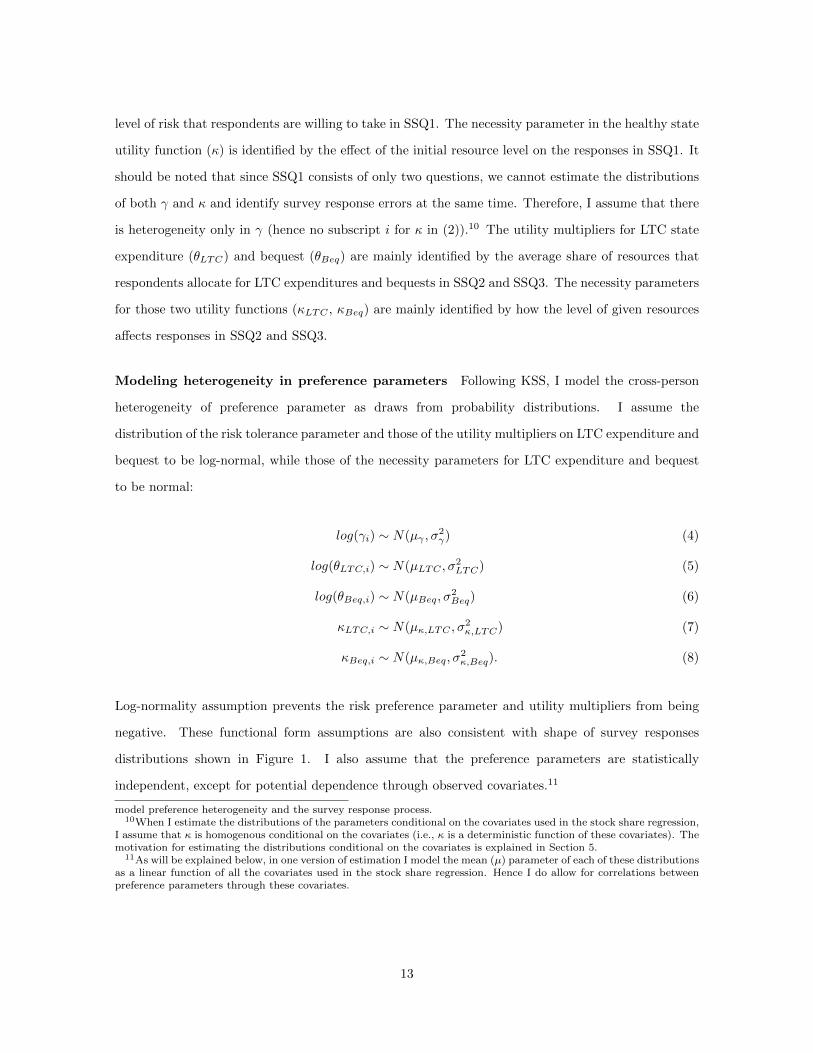
in the LTC state is higher, the optimal stock share is lower. The effects of both θBeq and κBeq show

that a stronger bequest motive is associated with a lower stock share.

For all the parameters, the model predicts greater effects than found in the actual behavior of the

VRI sample. Increasing risk tolerance by two standard deviations in the model is associated with a

more than 40 percentage point increase in the stock share across wealth and income levels, compared

to the 3.2 percentage point increase found in the empirical analysis in Section 5. The heterogeneity

in the other parameters have smaller but still substantial effects. For example, heterogeneity in

precautionary saving motives for LTC, expressed as differences in θLTC , creates about a 7 percentage

point difference in the stock share for many wealth and income levels, while the difference can be as

large as 15 percentage points.26 The corresponding numbers for κLTC are much larger—10 percentage

points for many wealth-income combinations and more than 20 percentage points for some cases. Note

that the numbers from the empirical analysis were similar (though somewhat smaller) in the case of

θLTC (4.1 percentage points), while negligible for κLTC (1.7 percentage points). Finally, the effects

of heterogeneity in θBeq and κBeq are smaller compared to that of θLTC and κLTC , but in many

cases they are still larger than the numbers from the empirical analysis and the direction is actually

opposite to what the point estimates from the empirical analysis suggest.

I find almost the same pattern for age 80 (Figure 4). Overall, the size of the effect is reduced in

terms of percentage point differences, but this is mainly due to that older households have a lower

stock share than younger households because of the reduced value of human capital (see Figure 2(b)).

In terms of percent difference (not percentage point difference) in stock share, the effects have similar

magnitudes. Notice that the chance of having a negative health shock increases with age, but at the

same time the chance of having a long sequence of LTC shock (which is the most catastrophic event)

decreases due to increased mortality risk. Given that an LTC shock plays an important role in the

negative effect of both of the saving motives, as will be explained below, the similar results for the

age 55 and age 80 groups may reflect these factors canceling each other out for the older group.

6.2.2 Mechanisms Behind the Effects

Negative impact of a stronger LTC precautionary motive on the optimal stock share A

higher θLTC or lower κLTC means that households face larger background risk, since an endogenously-

26When the income level is high and the wealth level is low, the effect is zero, since for these households, under therange of values of θLTC used in this analysis, the optimal stock share is 100 percent. Large effect of heterogeneity inθLTC for these households will be obtained if I allow for leveraging. The same caveat applies to the analyses for theother preference parameters.

26

determined LTC expenditure is larger when households are hit by an LTC shock. Therefore, those

with higher θLTC or lower κLTC want to reduce their exposure to financial market risk.

For those who do not have enough resources, the availability of publicly-funded LTC service reduces

this effect. This fact is well demonstrated in the effect of κLTC at age 80. For the low-wealth and

low-income combination, larger required expenditures in the LTC state (i.e., lower κLTC) is associated

with a higher optimal stock share (see Figure 4(e)). When both the wealth and income levels are low,

and if they are going to spend significant money on LTC service when they are hit by a LTC shock,

it is more likely that they will end up using the option of a public LTC service. Consequently, this

household would be less affected by the combination of a negative stock return shock and an LTC

shock since it would forfeit its wealth anyway upon choosing to use the public LTC service.

Negative impact of a stronger bequest motive on the optimal stock share The negative

effect of a stronger bequest motive on the optimal stock share, in particular that of θBeq, may seem

puzzling given that the medium value of κBeq is positive. Since a bequest is a luxury good, higher

weight on the bequest motive should imply lower effective risk aversion. Ding, Kingston, and Purcal

(2014) have a similar finding in an environment without health and mortality risks and income.

The negative effect comes from the two elements of the model: the existence of retirement income

and LTC risk under the presence of mortality risk. First, to understand the role played by the

retirement income, suppose that a household that invested its entire wealth in stocks experiences

a negative ten percent stock return. If that household has mainly been saving to finance its own

consumption rather than to bequeath its wealth, this loss of stock value will not translate into a

ten percent reduction in permanent consumption as long as the household has significant retirement

income from either Social Security or defined benefit pensions, which is not affected by the stock

market performance. If that household has mainly saved to leave bequests, however, the loss in

stock value can be translated into about a ten percent reduction in bequests, in particular when the

household dies soon after that, because unrealized retirement income cannot be bequeathed. In short,

the existence of unrealized retirement income and mortality risk can increase the effective risk of a

negative stock market return for those with stronger bequest motives.27

Second, the effective risk of the same LTC shock is larger for a household with larger θBeq because

when a household is hit by a LTC shock, the amount of wealth that can be bequeathed is dramatically

27It is clear that the size of this effect should depend on the replacement rate (λ) of retirement income. Hence, wecan predict that the transition from a DB-pension to a DC-pension system should reduce the effect of this channel.

27

reduced and, at the same time, mortality risk is increased. They would not have enough time to

accumulate their wealth again until they die. For those who mainly care about their own consumption

(i.e., those with lower θBeq), however, the fact that an LTC shock accompanies the increase mortality

risk is functioning as an insurance since the chance that they will outlive their resources is reduced

with the higher mortality risk.

To measure the effect of an LTC shock on bequests, I ran 10,000 simulations for each value of θBeq

and calculated the average bequest conditional on the age at death, θBeq, and also on whether the

household ever had an LTC shock in its lifetime or not (see Section 6.2.3 for details on the setup of

the simulations). Figure 5(a) shows the result. (Figure 5(b) plots the survival rate up to each age to

show the likelihoods of dying at different ages.) Having an LTC shock in their lives reduces bequests

on average about $100K for all the θBeq values and for most of ages at death, while the effect gets

larger for those whose age at death is higher than 95. In terms of proportion rather than absolute

value, the size of the shock on bequest gets larger as they die at higher ages. And this shock is more

painful to those with high θBeq values.

To test the strength of these channels, I shut off LTC and bequest risks and revisit the effect of

θBeq (Figure 5(c)). In the absence of these risks, we see that the stronger bequest motive implies

higher stock share, as in Ding, Kingston, and Purcal (2014), though the effect is in general very small.

Small effect of bequest motive Though a strong bequest motive lowers the optimal stock share,

overall the size of the effect is not large. To investigate the reason for this small effect, in Figure 6

I separately calculate the effect of one-standard-deviation differences of θBeq in its lower range (low

θBeq - medium θBeq) and higher range (medium θBeq - high θBeq). The figure shows that the effect of

θBeq is non-linear: the effect is almost null until it becomes large enough. Almost the entire effects of

two-standard-deviation differences in θBeq are from the one-standard deviation differences in its higher

range. Since the median LTC precautionary saving motive is already strong enough to leave sizeable

accidental bequests as long as they do not live up to very high ages and/or they are not hit by a long

sequence of LTC shocks, when the bequest motive is not strong, it is already saturated with these

accidental bequests. This can be seen from the fact that one-standard-deviation difference in θBeq

in its lower range does not affect the accumulation of wealth and hence in the amount of accidental

bequests (Figure 5(a)). Once θBeq is large enough, it starts to affect both wealth accumulation and

portfolio allocation.

28

6.3 Life-Cycle Profile of Stock Share

To summarize the effect of the preference heterogeneity on stock share of households over life-

cycle, I generate life-cycle profiles of stock share by simulating the model to investigate the model’s

implications for the design of life-cycle financial advice. For each combination of parameter values

considered in Figure 3 and 4, I simulate 10,000 households using the policy functions for saving and

portfolio choices and then take the average to obtain the profiles. The simulation starts from age 55

with a wealth level of $700K. I set y to be $90K. In Figure 6, I show profiles across different θLTC

(Panel (a) and (b)) and θBeq (Panel (c) and (d)).

In Panel (a) I first show the average wealth profile since different preference parameter values affect

wealth-to-income ratio and the latter, in turn, affects the optimal stock share. Households accumulate

wealth before retirement (age 65) and then decumulate afterward. With a stronger precautionary

saving motive associated with LTC (i.e. higher θLTC), the accumulation rate is faster while the

decumulation rate is slower, leading to an overall higher wealth level.

Accumulation of wealth and approaching retirement together can explain the downward sloping

stock share profile before retirement depicted in Panel (b). In this phase, the slope is the same across

different values of θLTC . Furthermore, the profile in this phase is fairly close to the often-mentioned

rule of thumb for life-cycle funds, which says that stock share in terms of percentage should be

determined by subtracting one’s age from 100.

After retirement, however, the slope depends on the strength of the precautionary saving motive.

At the median preference, the slope becomes flat after retirement. With a strong precautionary saving

motive for LTC, the slope is negative; the opposite is true when this saving motive is weak. Differences

in the slopes, again, mainly reflect differences in the wealth-to-human-capital ratio across different

groups. Those with a stronger precautionary saving motive for LTC save more, and an increased

wealth-to-human-capital ratio implies a lower stock share.

Panel (c) and (d) show that I obtain similar results over θBeq. One noticeable difference is that

until θBeq becomes large enough, the effect of that preference parameter on both wealth accumulation

and portfolio allocation is limited, given the strength of the median precautionary saving motive for

LTC.

This exercise shows that there is no uniform rule for stock share adjustment over the life-cycle that

can be applied to every household. The rules, on the one hand, should consider differences in optimal

stock share, given wealth level, across households with different motivations for saving (reflected in

29

different initial levels of stock share profiles in Figure 7(b) and 7(d)), and on the other hand, the

rules should also consider different wealth-to-human capital ratios that result from the heterogeneity

in motivations for saving (reflected in different slopes of stock share profiles in Figure 7(b) and 7(d)).

7 Conclusion

I find evidence that both the preferences for LTC expenditures and bequests are overall strong but

also heterogeneous across households. The former implies that older households are on average

substantially exposed to health-related risks including LTC risk and mortality risk, while the latter

implies that there is large heterogeneity in their exposures to these risks. The life-cycle portfolio choice

model with the estimated preference heterogeneity predicts that the optimal stock share is lower for

a household with either a stronger LTC precautionary saving motive or a stronger bequest motive. I

find a qualitatively similar pattern in the relationship between the households’ actual stock share and

the estimated preference parameters. The size of the response, however, turns out to be much smaller

than the prediction from the model.

This paper has three broad findings concerning LTC risk. First, the interaction of LTC risk and

health-dependent utility substantially affects portfolio choice and wealth accumulation in an otherwise

standard life-cycle model. Second, there is substantial heterogeneity in preferences for spending in

the LTC state. Put together, these findings imply that household portfolio choices should be strongly

affected by these preferences and should vary across households in accordance with their preferences.

The third finding, however, is that in a large sample of households with sufficient financial resources

where these choices and risks should be highly relevant, the actual response of portfolios to preference

heterogeneity is in the direction implied by the life-cycle model, but substantially attenuated relative

to the predictions from the model. One possible reason for this low-powered response of choices

to the stated preference is that financial advice does not sufficiently take into account of LTC risk.

This risk can take the form either of high probability of needing LTC or, as this paper emphasizes,

preference for large spending should LTC be needed. The theoretical findings of this paper imply that

portfolio advice should be conditioned on these preferences and risks. The paper, by documenting the

heterogeneity in preferences and by showing its implications for portfolios for households in different

circumstances, provides a roadmap for improving the financial advice to and financial products for

households who need to manage financial assets during retirement while facing multiple risks.

30

References

[1] Ameriks, John, Joseph Briggs, Andrew Caplin, Matthew D. Shapiro, and Christopher Tonetti

(2015a): “Long-Term Care Utility and Late in Life Saving,” Vanguard Research Initiative

Working Paper.

[2] Ameriks, John, Joseph Briggs, Andrew Caplin, Matthew D. Shapiro, and Christopher Tonetti

(2015b): “Late-in-Life Risks and the Under-Insurance Puzzle,” Vanguard Research Initiative

Working Paper.

[3] Ameriks, John, Andrew Caplin, Steven Laufer, and Stijn van Nieuwerburgh (2011): “The Joy

of Giving or Assisted Living? Using Strategic Surveys to Separate Public Care Aversion from

Bequest Motives,” Journal of Finance, 66, 519-561.

[4] Ameriks, John, Andrew Caplin, Minjoon Lee, Matthew D. Shapiro, and Christopher Tonetti

(2014): “The Wealth of Wealthholders,” Vanguard Research Initiative Working Paper.

[5] Barsky, Robert B., F. Thomas Juster, Miles S. Kimball, and Matthew D. Shapiro (1997):

“Preference Parameters and Behavioral Heterogeneity: An Experimental Approach in the Health

and Retirement Study,” Quarterly Journal of Economics, 112, 537-579.

[6] Benzoni, Luca, Pierre Collin-Dufresne, and Robert S. Goldstein (2007): “Portfolio Choice over

the Life-Cycle when the Stock and Labor Markets are Cointegrated,” Journal of Finance, 62,

2123-2167.

[7] Berkowitz, Michael K. and Jiaping Qiu (2006): “A Further Look at Household Portfolio Choice

and Health Status,” Journal of Banking and Finance, 30, 1201-1217.

[8] Berndt, Ernst R., Bronwyn H. Hall, Robert E. Hall, and Jerry A. Hausman (1974): “Estimation

and Inferences in Nonlinear Structural Models,” Annals of Economic and Social Measurement,

3, 653-665.

[9] Bodie, Zvi, Robert C. Merton, and William F. Samuelson (1992): “Labor Supply Flexibility

and Portfolio Choice in a Life Cycle Model,” Journal of Economic Dynamics and Control, 16,

427-449.

31

[10] Brunnermeier, Markus K. and Stefan Nagel (2008): “Do Wealth Fluctuations Generate Time-

Varying Risk Aversion? Micro-Evidence on Individuals Asset Allocation,” American Economic

Review, 98, 713-736.

[11] Campbell, John Y. (2006): “Household Finance,” Journal of Finance, 61, 1553-1604.

[12] Campbell, John Y. and John H. Cochrane (1999): “By Force of Habit: A Consumption-Based

Explanation of Aggregate Stock Market Behavior,” Journal of Political Economy, 107, 205-251.

[13] Cocco, Joao F., Francisco J. Gomes, and Pascal J. Maenhout (2005): “Consumption and Portfolio

Choice over the Life Cycle,” Review of Financial Studies, 18, 491-533.

[14] De Nardi, Mariacristina, Eric French, and John B. Jones (2010): “Why Do the Elderly Save?

The Role of Medical Expenses,” Journal of Political Economy, 118, 39-75.

[15] De Nardi, Mariacristina, Eric French, and John B. Jones (2013): “Medicaid Insurance in Old

Age,” NBER Working Paper, 19151.

[16] Ding, Jie, Geoffrey Kingston, and Sachi Purcal (2014): “Dynamic Asset Allocation when

Bequests are Luxury Goods,” Journal of Economic Dynamics and Control, 38, 65-71.

[17] Fan, Elliott and Ruoyun Zhao (2009): “Health Status and Portfolio Choice: Causality or

Heterogeneity?” Journal of Banking and Finance, 33, 1079-1088.

[18] Finkelstein, Amy, Erzo F. P. Luttmer, and Matthew J. Notowidigdo (2009): “Approaches to

Estimating the Health State Dependence of the Utility Function,” American Economic Review,

99, 116-121.

[19] Goldman, Dana and Nicole Maestas (2013): “Medical Expenditure Risk and Household Portfolio

Choice,” Journal of Applied Econometrics, 28, 527-550.

[20] Gomes, Francisco and Alexander Michaelides (2003): “Portfolio Choice with Internal Habit

Formation: A Life-cycle Model with Uninsurable Labor Income Risk,” Review of Economic

Dynamics, 6, 729-766.

[21] Huang, Huaxiong and Moshe A. Milevsky (2008): “Portfolio Choice and Mortality-contingent

Claims: The General HARA Case,” Journal of Banking and Finance, 32, 2444-2452.

32

[22] Hurd, Michael D. (2002): “Portfolio Holdings of the Elderly,” In: Luigi Guiso, Michael Haliassos

and Tullio Jappelli (eds.), Households Portfolios, Cambridge: MIT Press, 27-54.

[23] Kimball, Miles S., Claudia R. Sahm, and Matthew D. Shapiro (2008): “Imputing Risk Tolerance

from Survey Responses,” Journal of the American Statistical Association, 103, 1028-1038.

[24] Klibanoff, Peter, Massimo Marinacci, and Sujoy Mukerji (2005): “A Smooth Model of Decision

Making Under Ambiguity,” Econometrica, 73, 1849-1892.

[25] Lockwood, Lee (2014): “Bequest Motives and the Choice to Self-Insure Late-Life Risks,” working

paper.

[26] Love, David A. and Paul A. Smith (2010): “Does Health Affect Portfolio Choice?”, Health

Economics, 19, 1441-1460.

[27] Manski, Charles F. and Francesca Molinari (2010): “Rounding Probabilistic Expectations in

Survey,” Journal of Business and Economic Statistics, 28, 219-231.

[28] Merton, Robert C. (1971): “Optimum Consumption and Portfolio Rules in a Continuous-Time

Model,” emphJournal of Economic Theory, 3, 373-413.

[29] Pang, Gaobo and Mark Warshawsky (2010): “Optimizing the Equity-Bond-Annuity Portfolio in

Retirement: The Impact of Uncertain Health Expenses,” Insurance: Mathematics and Economics,

46, 198-209.

[30] Polkovnichenko, Valery (2007): “Life-cycle Portfolio Choice with Additive Habit Formation

Preferences and Uninsurable Labor Income Risk,” Review of Financial Studies, 20, 83-124.

[31] Poterba, James, Steven Venti, and David Wise (2011): “The Composition and Drawdown of

Wealth in Retirement,” Journal of Economic Perspectives, 25, 95-118.

[32] Reichling, Felix and Kent Smetters (2015): “Optimal Annuitization with Stochastic Mortality

and Correlated Medical Costs,” American Economic Review, 105, 3273-3320.

[33] Rosen, Harvey S. and Stephen Wu (2004): “Portfolio Choice and Health Status,” Journal of

Financial Economics, 72, 457-484.

[34] Spaenjers, Christophe and Sven Michael Spira (2014): “Subjective Life Horizon and Portfolio

Choice,” HEC Paris Research Paper, No. FI-2013-985.

33

[35] Viceira, Luis M. (2001): “Optimal Portfolio Choice for Long-Horizon Investors with Nontradable

Labor Income,” Journal of Finance, 56, 433-470.

[36] Vissing-Jorgensen, Annette (2002): “Towards an Explanation of Household Portfolio Choice

Heterogeneity: Nonfinancial Income and Participation Cost Structures,” NBER Working Paper

8884.

[37] Wachter, Jessica A. and Motohiro Yogo (2010): “Why Do Household Portfolio Shares Rise in

Wealth?” Review of Financial Studies, 23, 3929-3965.

34

Table 1: Summary Statistics

PercentilesMean 10 25 50 75 90

Stock Share 0.548 0.189 0.378 0.553 0.743 0.905Coupled 0.673Male 0.647Age 68.0 58 62 67 73 78Employer- 0.219sponsored sampleHealth (≥ Good) 0.948Education 0.404(Post college)Education 0.330(College)Income($) 126,132 28,740 50,000 83,443 125,000 250,000Financial Wealth ($) 1,101,468 153,000 344,000 723,665 1,356,211 2,399,317Prob. need LTCa 0.430 0.05 0.15 0.45 0.75 0.85Prob. live approx. 0.753 0.45 0.65 0.85 0.95 0.9510 more yearsb

Having LTC 0.234insurance

Notes: The tabulation is conditioned on having responses to all the variables used in this paper (all theSSQs in addition to the variables in this table). N=5,471.a The subjective probability of being in need of a LTC service at least for 1 year in the remaining life.b The subjective probability of living up to at least age min({75, 85, 95} ∩ {t|t ≥ age+ 5}). For example,for a respondent whose age is 75, it is the probability of living up to age 85.

35

Table 2: Estimated Distributions of the Preference Parameters and Survey Response Errors

(a) Estimated distribution parameters

Parameter Estimate S.E.µγ -1.322 (0.013)σγ 0.691 (0.007)κ -10.82K (0.43K)µLTC 1.292 (0.034)σLTC 2.317 (0.029)µκ,LTC -35.97K (0.64K)σκ,LTC 24.67K (0.29K)µBeq 2.487 (0.042)σBeq 3.548 (0.047)µκ,Beq 38.74K (1.11K)σκ,Beq 45.10K (0.69K)σε11 0.177 (0.002)σε12 0.109 (0.001)σε21 14.98K (0.14K)σε22 11.98K (0.15K)σε23 8.11K (0.09K)σε31 15.24K (0.14K)σε32 9.84K (0.17K)σε33 19.33K (0.25K)N 5,471Log-likelihood -125,903

(b) Implied distributions of preference parameters

PercentilesParameter 10 25 50 75 90 Meanγi 0.11 0.17 0.27 0.43 0.65 0.34θLTC,i 0.19 0.76 3.64 17.37 70.91 53.32θBeq,i 0.12 1.10 12.03 131.65 1134.69 6510.37κLTC -67.59K -52.61K -35.97K -19.33K -4.35K -35.97KκBeq -19.06K 8.32K 38.74K 69.16K 96.54K 38.74K

36

Table 3: Stock Share Regression: Using Raw Responses to SSQs

1 2SSQ1 (10-20%) 0.028*** 0.016

(0.010) (0.010)SSQ1 (20-33%) 0.048*** 0.034***

(0.010) (0.010)SSQ1 (33-50%) 0.059*** 0.046***

(0.012) (0.012)SSQ1 (50-75%) 0.081*** 0.070***

(0.013) (0.013)SSQ1 (75-100%) 0.037 0.037

(0.026) (0.026)SSQ2 -0.048** -0.034*(Share of wealth for LTC) (0.020) (0.020)SSQ3 0.008 0.015(Share of wealth for bequest) (0.015) (0.015)Coupled -0.017**

(0.008)Male 0.024***

(0.008)Age -0.000

(0.001)Employer-sponsored -0.046***

(0.009)Health (Good) -0.020

(0.016)Post college degree 0.034**

(0.015)College degree 0.027*

(0.014)Log income 0.014***

(0.005)Log wealth 0.015***

(0.004)LTC prob. -0.023**

(0.012)Longevity prob. 0.044***

(0.017)LTCI -0.013

(0.008)N 5471 5471R2 0.011 0.031

Note: For SSQ1, the most risk averse category (i.e., willing to risk0-10% of their income to have a 50% chance of doubling income)is the omitted category. For SSQ2 the raw response is defined asthe share of wealth the respondent allots for the LTC state, aver-aged over the three questions. For SSQ3, it is the share of wealthbequeathed, averaged over the three questions. For a descriptionof the controls, see the note to Table 1.*= p<0.1, **=p<0.05, ***=p<0.01

37

Table 4: Stock Share Regression: Using Estimated Preference Parameters (Cardinal Proxies)

1 2logγ 0.027*** 0.023***

(0.006) (0.006)logθLTC -0.010*** -0.009***

(0.002) (0.002)logθBeq 0.002 0.001

(0.002) (0.002)κLTC 0.034 0.038(in $100K) (0.023) (0.023)κBeq -0.029* -0.010(in $100K) (0.015) (0.016)Coupled -0.016

(0.010)Male 0.014

(0.011)Age -0.000

(0.001)Employer-sponsored -0.036**

(0.015)Health (Good) -0.011

(0.020)Post college degree 0.020

(0.018)College degree 0.020

(0.016)Log income 0.012*

(0.007)Log wealth 0.015***

(0.005)LTC prob. -0.032***

(0.010)Longevity prob. 0.035*

(0.019)LTCI -0.011

(0.008)N 5471 5471R2 0.009 0.029

Note: See Section 4 for construction of the cardinal prox-ies. For a description of the controls, see the note to Ta-ble 1. Standard errors are bootstrapped, with 100 repe-titions.*= p<0.1, **=p<0.05, ***=p<0.01

38

Table 5: Implied Changes in Stock Share by a Two-standard-deviation Increase in Each PreferenceParameters

1 2(without control) (with control)

logγ 0.037 0.032logθLTC -0.046 -0.041logθBeq 0.012 0.011κLTC 0.017 0.019κBeq -0.026 -0.009

Table 6: Calibration of Parameters for Baseline Model

(a) Heterogeneous preference parameters

Parameter Valueγ High 0.53

Medium 0.27Low 0.13

θLTC High 36.93Medium 3.64

Low 0.36θBeq High 418.80

Medium 12.03Low 0.34

κLTC High -11.30KMedium -35.97K

Low -60.64KκBeq High 83.84K

Medium 38.74KLow -6.36K

Note: For each parameter, medium value is the mean value of the distribution (exponential of meanif the distribution of the parameter is log-normal) while high (low) value is the mean plus (minus)one standard deviation (again exponential of those values if the distribution of the parameters islog-normal).

(b) Other parameters

Parameters Value Target/Sourceκ -10.82K VRI estimationβ 0.96 StandardPC −κLTC + 10K Ameriks et al. (2015b)πss′ HRS estimationRf 1.02 Cocco et al. (2005)ση 0.17 Cocco et al. (2005)µs 0.02 VRI stock share levely {$45K, $90K, $120K} VRI dataλ 0.5 VRI dataσ2nu 0.07 Cocco et al. (2005)

39

Figure 1: Distribution of Responses to SSQs

(a) SSQ1

Note: Risk categories show the downside risk that is accepted for a 50 percent

chance of doubling income. 0-10% is the most risk averse group while 75-100% is

the most risk tolerant one.

(b) SSQ2

40

(c) SSQ3

41

Figure 2: Stock Share Policy Functions (under the median preference parameters)

(a) Age 55

(b) Age 80

Note: Figure shows the optimal stock share policy function for healthy males, under various values of

average income and median preferences. The horizontal axis is financial wealth at the beginning of the

period (in $1,000s), and the vertical axis is the optimal stock share.

42

Figure 3: Effects of Heterogeneous Preference Parameters on Optimal Stock Share (age 55, healthy,male)

(a) Effect of γ

(b) Effect of θLTC

43

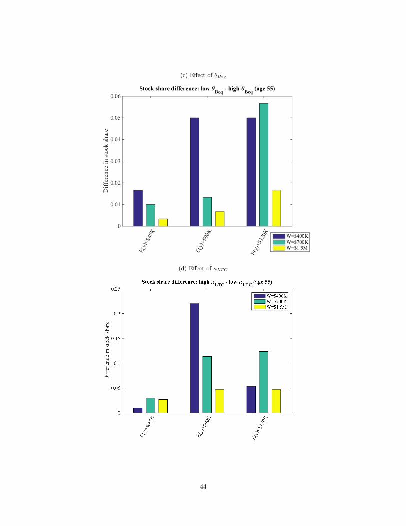
(c) Effect of θBeq

(d) Effect of κLTC

44

(e) Effect of κBeq

Note: Figure shows the difference in the optimal stock share across different values for preference

parameters, under various wealth and mean income levels, at age 55 for healthy males.

45

Figure 4: Effects of Heterogeneous Preference Parameters on Optimal Stock Share (age 80, healthy,male)

(a) Effect of γ

(b) Effect of θLTC

46

(c) Effect of θBeq

(d) Effect of κLTC

47

(e) Effect of κBeq

Note: Figure shows the difference in the optimal stock share across different values for preference

parameters, under various wealth and mean income levels, at age 80 for healthy males.

48

Figure 5: Mechanism Behind the Effect of θBeq

(a) Effect of LTC shock on bequests

Note: Figure shows the average amount of bequest conditional on age at death, θBeq, and whether the

household ever had LTC shock during its lifetime. Averages are calculated from 10,000 simulations for each

θBeq value. Each simulation starts with wealth of $700,000 and y = $90, 000.

(b) Survival rate

49

(c) Effect of θBeq under no health-related risks

Note: Figure shows the difference in the optimal stock share across different values of θBeq under no LTC

risk and mortality risk. A household lives up to age 110 and then dies with probability one. The figure is

drawn for healthy males at age 55, with y = $90, 000, under various wealth levels.

50

Figure 6: Effect of one-standard-deviation difference in θBeq

(a) Limited effects in the lower range of θBeq

(b) Larger effects in the higher range of θBeq

Note: Figure is constructed in the same way as in Figure 5(c), but in this Figure I calculate the effect of

one-standard-deviation differences in θBeq.

51

Figure 7: Life-cycle profiles for wealth and stock share under various θLTC and θBeq

(a) Wealth with various θLTC

(b) Stock share with various θLTC

52

(c) Wealth with various θBeq

(d) Stock share with various θBeq

Note: Figure shows the life-cycle profiles of wealth and stock share under various values of θLTC and θBeq.

Profiles are calculated from 10,000 simulations for each parameter value. Each simulation starts with wealth

of $700,000 and y = $90, 000.

53

A Appendix: Details on Strategic Survey Questions (SSQs)

Table A1 shows the exact wordings and parameter values used for each type of SSQ. Each type is

asked multiple times with different amounts of given resources (W ) and/or different likelihoods of

relevant events (π).

Figure A1 shows an example of the interface—a bar with a slider—that is used in SSQ2 and SSQ3

to help respondents understand the underlying trade-off in allocating their resources. In this figure, a

respondent is answering the first question of SSQ2 (allocating $100,000 between Plan C and Plan D,

where the chance of needing a LTC service in the next year is 25%). When the respondent first sees

this screen, it does not have a slider and there is only an empty bar. Once the respondent clicks on

the bar, the slider appears where she clicked. The purpose of this design is to prevent any anchoring

effect of an arbitrarily-chosen initial location. After the initial click, the respondent can move the

slider to the left and right to adjust the allocation. Whenever the slider is moved, the numbers below

the bar, which show the amount of resources available for each state under the current allocation,

automatically update. In this way, the respondent can see the consequence of her decision without

needing to make complex calculations.

54

Table A1: Strategic Survey Questions

(a) SSQ1 (Risk tolerance)

Set up Suppose you are 80 years old. Suppose, further, that for the next year:• You live alone, rent your home, and pay all your own bills.• You are in good health and will remain in good health.• You will have no medical bills or other unexpected expenses.• You do not work.

Hypothetical • Plan A guarantees that you will have $W for spending next year.financial • Plan B will possibly provide you with more money, but is less certain.products There is a 50% chance that Plan B would double your money, leaving you with $2W ,

and a 50% chance that it would cut it by x%, leaving you with $(1− 0.01× x)W .Rules • You have no other assets or income, and so the only money you have available for all your

spending next year is from either Plan A or Plan B.• Any money that is not spent at the end of next year cannot be saved for the future.• You cannot give any money away or leave it as a bequest.• If you need anything next year, you have to pay for it. No one else can buy anything for you.• At the end of next year you will be offered the same choice with another $W for following year.

Parameters W = $100, 000 and $50, 000.asked

(b) LTC-state utility function

Set up • You are 80 years old, live alone, rent your home, and pay all your own bills.• There is a π chance that you will need help with ADLs for all of next year.• There is a (1− π) chance that you will not need any help at all with ADLs for all of next year.• You have $W to divide between two plans for the next year.• At the end of next year you will be offered the same choice with another $W for following year.

Hypothetical • Plan C is hypothetical ADL insurance that gives you $(1/π) for each dollar invested if you dofinancial need help with ADLs.products • Plan D gives you $1 for each dollar invested only if you do not need help with ADLs.Rules • You can only spend money from Plan C or Plan D next year. You do not have any other money.

• Any money that is not spent at the end of next year cannot be saved for the future, given away,or left as a bequest.• Regardless of whether or not you need help with ADLs, your hospital, doctor bills, and

medications are completely paid by insurance.• Other than Plan C, you have no other resources available to help with your long-term care.

You have to pay for any long-term care you may need from Plan C.• There is no public-care option or Medicaid if you do not have enough money to pay for

a nursing home or other long-term care.• An impartial third party that you trust will verify whether or not you need help with ADLs

immediately, impartially, and with complete accuracy.Parameters (W,π) = ($100, 000, 25%), ($100, 000, 50%), and ($50, 000, 25%).asked

55

(c) SSQ3 (Bequest utility function)

Set up • You are 85 years old, live alone, rent your home, and pay all your own bills.• You know with certainty that you will live for only 12 more months and that you will need

help with ADLs for the entire 12 months.• You have $W to split into the following two plans.

Hypothetical • Plan E is reserved for your spending. From Plan E, you will need to pay all of your expenses,financial including long-term care and any other wants, needs, and discretionary purchases.products • Plan F is an irrevocable bequest.Rules • You have no money other than $W .

• No one—including friends or family—can take care of you for free. Long-term care must bepurchased at market rates.• Any money in Plan E that you do not spend cannot be given away or left as a bequest.• Bequests from Plan F are not subject to any taxation.• You have full insurance that covers all of your hospital, doctor, and medications, but you have

no long-term care insurance.• There is no public-care option or Medicaid if you do not have enough money to pay for a nursing

home or other long-term care.Parameters W = $100, 000, $150, 000, and $200, 000.asked

56

Figure A1: Example of the SSQ Interface

57

B Appendix: Estimation of Preference Parameter

Distribution Conditional on Covariates

Table B1 shows the results from the estimation conditional on the covariates. For most of the

covariates, they have offsetting effects on the multiplier and the necessity parameter so their effect

on each saving motivation is ambiguous. For example, for more educated respondents, the utility

multiplier for the LTC state tends to be smaller while the corresponding necessity parameter tends to

be more negative (i.e., the minimum expenditure in the LTC state increases).

The following variables have unambiguous effects on the saving motives. Older respondents tend

to be more risk averse. They also have a stronger precautionary saving motive for LTC and a

stronger bequest motive. The strength of the bequest motive is also associated with a more pessimistic

expectation regarding their own health (both LTC and longevity expectations) and a lower income

level.

58

Table B1: Estimated Distributions of the Preference Parameters and Survey Response Errors,Conditional on Covariates

Preference Parametersµγ κ µLTC µκ,LTC µBeq µκ,Beq

Constant -1.147*** -12.473* 2.693*** -16.710 4.140*** 16.937(0.214) (7.192) (0.558) (10.242) (0.761) (16.451)

Coupled -0.025 2.594*** 0.077 2.704** 0.641*** 1.498(0.025) (0.883) (0.072) (1.210) (0.088) (1.678)

Male 0.239*** -1.475* -0.798*** -9.527*** -0.579*** -15.097***(0.023) (0.849) (0.071) (1.238) (0.091) (1.731)

Age -0.003* -0.118* 0.033*** -0.099 0.032*** -0.352***(0.002) (0.061) (0.005) (0.079) (0.006) (0.122)

Employer-sponsored -0.108*** 6.624*** 0.496*** 12.407*** 0.424*** 0.596(0.030) (1.147) (0.077) (2.077) (0.097) (2.127)

Health (≥Good) -0.219*** 8.963*** 0.489*** 14.679*** 1.238*** 18.509***(0.049) (1.491) (0.162) (2.077) (0.200) (2.607)

Post college degree 0.205*** -9.270*** -0.778*** -15.812*** -0.741*** -10.092***(0.037) (1.543) (0.114) (2.192) (0.152) (3.443)

College degree 0.085** -5.000*** -0.558*** -7.088*** -0.558*** -7.771**(0.034) (1.497) (0.103) (2.102) (0.145) (3.300)

Log income 0.015 -0.589 -0.261*** -2.211** -0.277** 0.209(0.014) (0.494) (0.029) (0.734) (0.054) (1.263)

Log wealth -0.028*** 0.113 0.027 1.851*** -0.084** -5.913***(0.011) (0.400) (0.025) (0.560) (0.034) (0.795)

LTC prob. 0.061* -1.726 -0.296** -12.479*** 0.409*** -7.569***(0.034) (1.177) (0.102) (1.674) (0.122) (2.344)

Longevity prob. 0.316*** -7.851*** -0.650*** -11.733*** -0.861*** 3.876(0.046) (1.728) (0.143) (2.383) (0.174) (3.680)

LTCI -0.119*** 3.590*** -0.199** -2.340* -0.173* -2.961(0.025) (0.952) (0.089) (1.314) (0.105) (1.910)

Heterogeneityσ 0.679*** n/a 2.286*** 24.599*** 3.530*** 43.332***

(0.007) (0.029) (0.405) (0.046) (0.674)Measurement errorσε11 0.176***

(0.002)σε12 0.109***

(0.001)σε21 14.660***

(0.138)σε11 11.834***

(0.147)σε11 7.994***

(0.091)σε11 15.081***

(0.147)σε11 9.703***

(0.164)σε11 19.204***

(0.234)Log-likelihood -125,659

59

C Appendix: Distribution of Expenditure Shares from a

Static Problem

To show the implications of the estimated parameter distributions more clearly, following Ameriks,

Briggs, Caplin, Shapiro, and Tonetti (2015a), I conduct the following exercise. I assume the following

maximization problem:

Maxx1,x2(x1 − κ)1−1/γi

1− 1/γi+ θLTC,i

(x2 − κLTC,i)1−1/γi1− 1/γi

+ θBeq,i(W − x1 − x2 − κBeq,i)1−1/γi

1− 1/γi

s.t. 0 ≤ x1, x2,≤W(C.1)

which is a static problem with no uncertainty. The household should divide the given resource W

into three expenditures: expenditures in the healthy state (x1), expenditures in the LTC state (x2),

and bequests (W − x1 − x2). Although this problem is unrealistic, the solution can demonstrate the

strength of each saving motivation under the estimated parameters. For each individual, I solve (C.1)

under W = $400K and $1M and the proxy values of the preference parameters.28

In Figure C1, I show the distribution of expenditure shares. Under W = $400K, many respondents

spend more than 40 percent of their wealth for expenditure in the LTC state. About 30 percent of

respondents do not leave any bequests. Not many respondents spend a large fraction of their resources

in the healthy state. When they have more resources (W = $1M), the share of expenditure in the

LTC state tends to go down while the share of bequest tends to go up. These changes are driven

by the differences in the necessity parameters, which make, on average, bequests luxury goods, and

expenditures in the LTC state necessary goods.

28For the parameters that are assumed to have log-normal distribution, I take the expectation of log of the parametersand take the exponential of it, to avoid Jensen’s inequality. The proxy calculated in this way matches the median ofthe estimated distribution, though it misses the mean, in terms of the level of the parameter. Furthermore, sincethe proxies are calculated as conditional expectations, it has mean reversion compared to the estimated distribution.Hence plugging these proxies directly into (C.1) would yield less heterogeneity in saving motives compared to what theestimated distributions imply. To correct this problem, in the case of log-normally distributed parameters, before I takeexponential of the conditional expectation of the log of the parameter, I convert it by logh′ = logh + (logh − µθ) σθ

σhwhere logh is the expected value of the log of the parameter, µθ is the estimated mean of the log-normal distribution,σh is the standard deviation of logh and σθ is the estimated standard deviation of the log-normal distribution. ThenI take the exponential of logh′ to calculate cardinal proxies for this exercise. For normally distributed parameters, Iapply the same procedure except for that log operators are dropped in the above formula and do not take exponentialat the end.

60

Figure C1: Distribution of Expenditure Share in the Static Problem

(a) Share of expenditure in the healthy state

(b) Share of expenditure in the LTC state

61

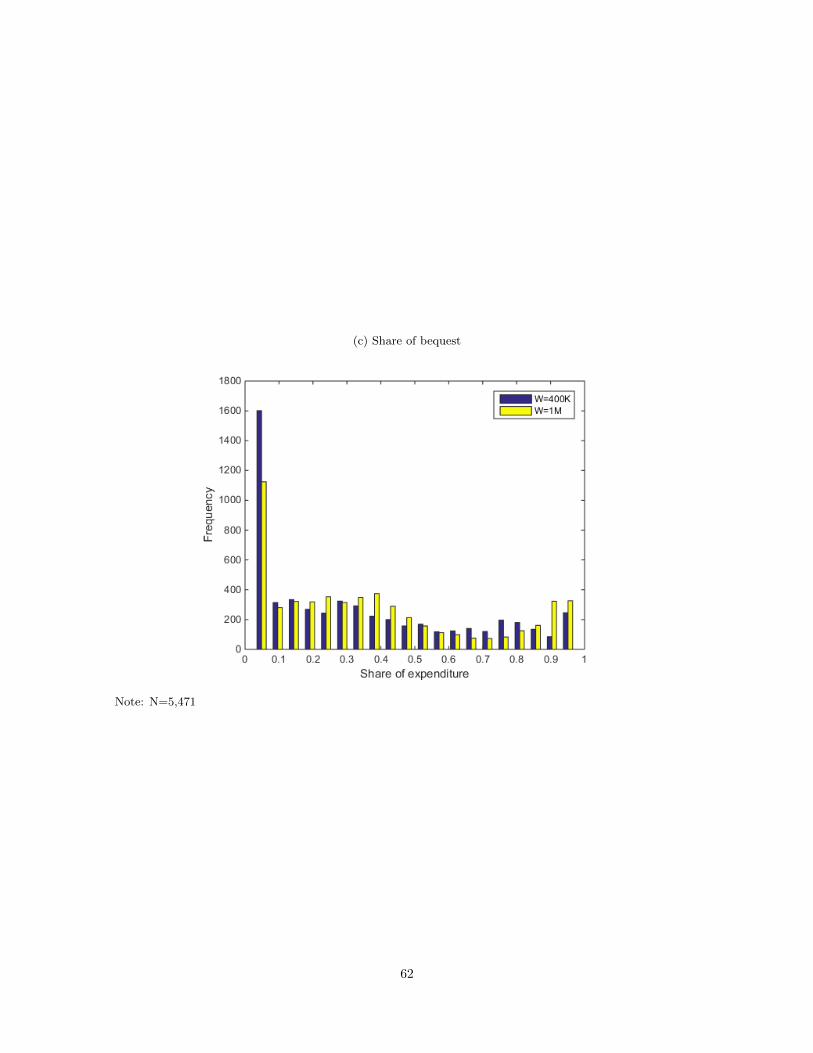
(c) Share of bequest

Note: N=5,471

62

D Appendix: Properties of the Cardinal Proxies Constructed

Based on the KSS Approach

In this appendix I explain how using cardinal proxies, constructed under the KSS approach, in place of

the true preference parameters can yield unbiased estimates in a linear regression.29 I also compare the

KSS method used in this paper and the individual-level estimation used in Ameriks, Briggs, Caplin,

Shapiro, and Tonetti (2015b).

Let θ denote the true preference parameter. When θ is observable, we can run the following

regression:

y = βθ + ε (D.1)

to estimate the relationship between dependent variable of interest (y) and θ. In this paper, I cannot

observe θ, so instead I use the proxy h = E[θ|R] where R represents responses to the survey questions.

Let u ≡ θ − h. Then the actual regression I am running is:

y = βh+ ν (D.2)

where ν = βu + ε. If u is a classical measurement error such that it is correlated with h, then h is

positively correlated with ν so the regression yields an attenuation bias. One important virtue of the

KSS approach—estimating the population distribution of the parameters first and then calculating

cardinal proxies as conditional expectations—is that the resulting cardinal proxy h is uncorrelated

with u by construction because h is the result of projection and u is the error term in that projection.

Instead, u is correlated with the true preference parameter θ.

To show this property visually, I run the following simulation. I assume that the true preference

parameter is distributed as log(θi) ∼ N(µ, σ2). I do not observe true preference parameter, but I

observe a survey response generated as Ri = θi + εi, εi ∼ N(0, σ2ε). I assume that µ and σ2 are

unknown while σ2ε is known. I estimate the unknown parameters using the KSS method and then

construct the cardinal proxy h for θ. Figure D1(a) shows the scatter plot of h and θ. Given any

level of h, distribution of observations is symmetric across the 45-degree line, showing that there is

no correlation between h and u. It is also clear that u is correlated with θ: for large values of θ

the observations are much more likely to be below the 45-degree line, while the opposite is true for

29This discussion is based on Kimball, Sahm, and Shapiro (2008).

63

small values of θ.30 This is because of mean reversion in h, which comes from the fact that h is

calculated as a conditional expectation. A downside of the KSS method is that, due to this mean

reversion, the proxy values should not be directly used to calibrate parameters at the individual level

in a heterogeneous agent model. The degree of heterogeneity in h is much smaller than the estimated

heterogeneity in the population distribution.

An alternative approach is the individual-level estimation used in Ameriks, Briggs, Caplin, Shapiro,

and Tonetti (2015b). The underlying model—utility functions and survey response generation

processes—is almost the same as that used in this paper. The main difference is that, instead of

estimating the population distribution of the parameters, it directly estimates preference parameters at

the individual level, using the responses of each individual only. The likelihood function is maximized

over individual preference parameters, not over moments of population distribution of the parameters.

The parameters estimated in this way can also be considered as the cardinal proxies (h) for the

parameters for each individual. One advantage of this approach is that it does not make any functional

form assumption for the population distribution. Also, there is no mean reversion in h since h is not

calculated as conditional expectation anymore. The absence of mean reversion makes the estimates

attractive for calibrating a heterogeneous agent model at the individual level as in Ameriks, Briggs,

Caplin, Shapiro, and Tonetti (2015b). One main disadvantage is that now h is positively correlated

with u, since survey response error directly affects both the point estimate (and hence the proxy) for

each individual and the difference between the proxy and the true parameter. The correlation between

h and u makes the estimates improper as regressors in a linear regression. Figure D1(b) shows the

scatter plot between h and u under the individual-level estimation, in the same exercise as in D1(a).

(In D1(b), h is nothing but R.) Under this method, u is uncorrelated with θ: given any level of θ,

the distribution of observations is symmetrical with respect to the 45-degree line. In contrast, this

distribution is correlated with h: for a large value of h the observations are more likely to be above

the 45-degree line and the opposite is true for a small value of h.

This discussion shows that the choice of the estimation method should be based on how estimates

will be used in the analysis.

30Note that in a linear regression that also has other covariates in the RHS, u can be correlated with those controlsthrough θ, resulting in biased estimates. To correct this, I make the mean of the parameter distributions (µ) a linearfunction of the controls that will be included in the second stage regression. This would enable us to obtain unbiasedestimates in that u would not be correlated with any of the controls or with the proxy.

64

Figure D1: Scatter plot of true parameter (θ) and cardinal proxy (h)

(a) KSS method

(b) Individual-level estimation

65

E Appendix: Estimation of Health State Transition Matrix

Using the HRS

I use an approach similar to that in De Nardi, French, and Jones (2013). To define health

status, I use the self-reported subjective health data from the HRS: s = G corresponds to

{Excellent, V ery Good, Good} in the subjective health report and s = B to {Fair, Poor}. As

long as a respondent reports that she requires help for at least one activity of daily living (ADL), then

she is classified as s = LTC.31 The transition to death (s = D) is identified with the exit report in

the HRS.

Let x be a vector that includes a constant, age, gender, and square of age and interactions of these

variables, as well as indicators for previous health status and previous health interacted with age. I

estimate a multinomial logit model, such that for i = {G,B,LTC} and j = {G,B,LTC,D},

πij = Pr(s′ = j|s = i)

= γij/∑

k∈{G,B,LTC,D}

γik

γiD ≡ 1, ∀i

γik ≡ exp(xβk), ∀i, k ∈ {G,B,LTC}

(E.1)

where {βk}k∈{G,B,LTC} are sets of coefficient vectors and of course Pr(s′ = D|s = D) = 1.

Note that what I need is an annual transition matrix while the HRS data have information on

biannual transitions. These two transition processes are linked, however, by:

Pr(s′′ = j|s = i) =∑k

Pr(s′′ = j|s′ = k)Pr(s′ = k|s = i)

=∑k

πkj,t+1πik,t

(E.2)

where the subscript t shows that the transition probability is a function of age (which is part of

x). (E.1) and (E.2) allow us to estimate {βk}k∈{G,B,LTC} directly from the data using maximum

likelihood estimation. The transition matrix is built on the estimated coefficients.

31This definition of the LTC state is the closest to that in the VRI survey.

66