Life-Cycle Asset Allocation: A Model with Borrowing

Constraints, Uninsurable Labor Income Risk and

Stock-Market Participation Costs∗

Francisco Gomes†

London Business School

and

Alexander Michaelides‡

University of Cyprus, London School of Economics and CEPR

January 2002

∗We would like to thank Lorenzo Forni, Luigi Guiso, Michael Haliassos, Pascal Maenhout, Monica Paiella,

Raman Uppal, Tan Wang and seminar participants at the May 2001 Asset and Liability Management Con-

ference at the University of Cyprus, the Ente-Einaudi Center, Leicester University and the LSE for helpful

comments and suggestions. The second author acknowledges funding from a University of Cyprus Research

grant and European Union funding through the HERMES Center. We are responsible for any remaining

errors or omissions.†Address: London Business School, Regent’s Park, London NW1 4SA, United Kingdom. Phone: (44)

2072625050. E-mail: fgomes@london.edu‡Address: Department of Economics, London School of Economics, Houghton Street, London, WC2A

2AE, United Kingdom. Email: A.Michaelides@lse.ac.uk.

1

Abstract

We study life-cycle asset allocation in the presence of liquidity constraints and undi-

versifiable labor income risk. We find that small stock-market entry costs can explain the

zero-median stockholding puzzle. Households start saving in the riskless asset and enter

the stock market later in life. Moreover, the presence of human capital rationalizes the

asset allocation puzzle of Canner, Mankiw and Weil (1997). Nevertheless, conditional on

participation, the portfolio allocation remains heavily skewed towards equities. Extensions

that generate a larger co-existence of cash and stocks imply a counterfactually high stock

market participation rate. These results suggest that simultaneously matching stock market

participation and asset allocation remains a challenge.

JEL Classification: G11.

Key Words: Life-Cycle Asset Allocation, Liquidity Constraints, Stock Market Participa-

tion Costs, Uninsurable Labor Income Risk.

1 Introduction

According to the most recent empirical evidence on life-cycle asset allocation, at least 50%

of the population (in any country) does not own equities. Stock-market participation rates

are very low among young households, and they increase significantly during working life.

Furthermore, even those households that do own equities, still invest a large fraction of their

financial wealth in alternative assets.1 These facts are at odds with the predictions of existing

life-cycle asset allocation models.

A seminal reference addressing the problem of portfolio choice over the life-cycle is

Samuelson (1969). Under the assumptions of independently and identically distributed re-

turns, homothetic preferences, and the absence of labor income, he concludes that the optimal

asset allocation should remain constant over time. However, in practice, labor income (or

human capital) constitutes a crucial asset for most households. To the extent that the level

and risk of the labor income stream change over the life-cycle, this can provide a rationale

for age-varying investment strategies. If markets are complete so that labor income risk can

be insured, its role is well understood from the seminal work by Merton (1971). However,

the incomplete markets case remained unsolved for many years.

Following Deaton (1991) and Carroll (1992), a large successful literature on buffer stock

saving with undiversifiable labor income risk has emerged.2 More recently these models have

been extended to include an asset allocation decision, both in an infinite-horizon setting (see

Haliassos and Michaelides (2002), Viceira (2001), Michaelides (2001), Heaton and Lucas

(2000, 1997 and 1996), Koo (1998), Lucas (1994) or Telmer (1993)) and in a finite-horizon

life-cycle setting (see Campbell, Cocco, Gomes and Maenhout (2001), Storesletten, Telmer

and Yaron (2001), Dammon, Spatt and Zhang (2001), Cocco, Gomes and Maenhout (1999),

Hochguertel (1999), or Gakidis (1998)).3

Consistent with the intuition in Jagannathan and Kocherlakota (1996), and with the1This evidence is discussed in more detail below.2See, for instance Cagetti (2001), Gourinchas and Parker (2001), Ludvigson and Michaelides (2001),

Carroll (1997), Carroll and Samwick (1997), or Hubbard, Skinner and Zeldes (1995).3Constantinides, Donaldson and Mehra (2001) and Bertaut and Haliassos (1997) analyze three period

models where each period amounts to 20 years.

3

recommendations offered by financial advisors (see for example, Malkiel, 1999), these mod-

els predict that the optimal share of wealth invested in equities is roughly decreasing during

(working) life.4 Nevertheless, as mentioned above, several important predictions of the model

are still at odds with empirical regularities. First, the zero median stock holding puzzle

(Mankiw and Zeldes (1991)) persists. The latest Survey of Consumer Finances reports that

only around 49 percent of US households hold stocks either directly or indirectly (through

pension funds, for instance). Yet, the frictionless portfolio choice model predicts that, given

the equity premium, all households should participate in the stock market as soon as saving

takes place. Second, in the model, households first enter the stock market and only later

decrease their exposure to stocks. This is a prediction that runs counter both to casual ob-

servation about stockholding patterns and to the evidence reported by Poterba and Samwick

(1999) and Ameriks and Zeldes (2001), who find that equity ownership increases with age,

at least until households reach retirement. Third, given the equity premium, households

invest almost all of their wealth in stocks, and this result is particularly stronger for young

households. Again, this is contrary to both casual empirical observation and more formal

evidence (see Poterba and Samwick (1999) or Ameriks and Zeldes (2001), for instance).

In this paper we attempt to improve the performance of the existing life-cycle asset alloca-

tion models with respect to these puzzles. We start by examining the potential for one-time,

fixed, stock market entry costs to generate significant non-participation. A large literature

has concluded that some level of fixed costs seems to be necessary to improve the empir-

ical performance of asset pricing models (see, among others, Brav, Constantinides, Geczy

(2002), Polkovnichenko (2000), Basak and Cuoco (1998), Vayanos (1998), Luttmer (1996,

1999), Heaton and Lucas (1996), He and Modest (1995), Aiyagari and Gertler (1991) or Con-

stantinides (1986)).5 With respect to asset allocation, empirical work by Vissing-Jorgensen4This intution can also be obtained from Merton (1971), in a complete markets setting.5In this paper we take a partial equilibrium approach thereby eliminating our ability to explicitly say

anything about asset pricing. However, the excessive demand for equities predicted by asset allocation

models, is the portfolio-demand manifestation of the equity premium puzzle. Therefore, to the extent that a

partial equilibrium model generates a more balanced portfolio which matches more closely the microeconomic

data on portfolio demands, we move closer towards building a general equilibrium model that could eventually

jointly match portfolio demands and asset returns.

4

(2002) and Paiella (1999) shows that small entry costs can rationalize the observed low

stock market participation rates6, while Attanasio, Banks and Tanner (2002) argue that

the implications of the Consumption Capital Asset Pricing Model cannot be rejected for

households predicted to hold both stocks and bonds (“shareholders”). However, Campbell,

Cocco, Gomes and Maenhout (2001) introduce such a fixed-cost in the life-cycle asset allo-

cation model, and find that it has a very small impact on the participation decision. On the

other hand, Haliassos and Michaelides (2002) argue that, in an infinite horizons model with

impatient households (as defined in Deaton (1991)), a small one-time entry cost can generate

stock market non-participation. In the infinite horizons model, the consumer/investor can

smooth idiosyncratic labor income risk by accumulating a small buffer of assets (Deaton,

1991), and therefore, the benefit from participating in the stock market is much lower.

Contrary to the results in Campbell et al. (2001), we find that small one-time stock mar-

ket participation costs can generate stock market entry later in life. The difference in the

results arises from changing (in plausible directions) the structural parameters that control

the strength of the precautionary savings motive. In particular, we reduce the coefficient

of relative risk aversion, thus weakening the desire to accumulate precautionary wealth bal-

ances. As a result, a small entry cost becomes important enough to generate stock market

participation only late in life, when sufficient wealth has been accumulated, making the

benefit strong enough to warrant paying the entry cost. More specifically, stock market

participation typically peaks at around ages 45− 65, depending on the parameters affectingthe precautionary savings motive and impatience. Given that surveys usually sample the

population between ages 25 and 75, we view this result as moving the model in the right di-

rection for explaining this puzzle. On the negative side, the model still predicts that, by age

65, all households will have paid the stock market cost and will have become stockholders.

Conditional on participation, the model still predicts (counterfactually) large equity hold-

ings. Motivated by this result, we consider three different extensions of the baseline model.

First, we increase background risk by allowing for a positive probability of a disastrous la-

bor income shock. In this case, the agent saves more, generating significant riskless asset6Degeorge, Jenter, Moel and Tufano (2002), estimate such a fixed-cost in the context of a specific even

study and obtain relatively modest values.

5

holdings, particularly for high values of risk aversion. However, the higher level of savings

induces a stronger incentive to enter the stock market, and therefore stock market partici-

pation takes place much earlier. The same result is obtained by increasing risk aversion, and

the intuition is again the same. From this analysis we conclude that other extensions along

the same lines, namely introducing consumption risk (taste shocks or housing, for instance)

or allowing for uncertainty about the parameters of the labor income process, will lead to the

same results: greater co-existence of cash and stocks in the portfolio but a counterfactually

high stock market participation rate over the life cycle on account of the higher level of

savings.

In our second extension we try to avoid this trade-off, by considering changes in the risk of

the stock-return process itself. In particular, we allow for large positive correlation between

stock returns and permanent earnings shocks, since the existing literature shows that this

will have a direct impact on the optimal portfolio allocation without significantly affecting

the consumption decision (Viceira (1999)), and therefore without increasing precautionary

saving. The model can generate large riskless asset holdings, but only for moderately large

levels of risk aversion, the ones for which we also obtain (counterfactually) large participation

rates. For low values of risk aversion the portfolio rule is only marginally changed, and

therefore the results are virtually the same as in the baseline case.

Finally we introduce a third financial asset in model, which we calibrate using data

on long-term government bonds. We find that, immediately after paying the fixed cost,

households invest almost all of their wealth in stocks. The desire to pay the fixed is motivated

by the willingness to hold stocks, not long-term bonds. As a result, the participation rate

(defined as percentage of households which have paid the fixed cost) is virtually the same as

in the 2-asset model. Nevertheless, for the households that have incurred the fixed cost, long-

term bonds become a substitute for cash. Specifically, the share of wealth invested in stocks

is not affected by the presence of this new asset, cash is replaced by bonds, and the share of

financial wealth allocated to cash drops almost to zero. These results rationalize the asset

allocation puzzle identified by Canner, Mankiw and Weil (1997): popular financial advisors

recommend that more risk-averse investors should allocate a higher fraction of their risky

portfolio (stocks plus bonds) to bonds. This is inconsistent with the predictions of the static

6

and frictionless Capital Asset Pricing Model which implies that all investors should hold the

same combination of risky assets; risk aversion only determines the size of the investment to

the risky assets as a whole. Brennan and Xia (2002 and 2000), Campbell, Chan and Viceira

(2002) and Campbell and Viceira (2001) show how this result can be derived in the context

of an intertemporal asset allocation model with time-varying expected returns. In this paper

we show that the presence of undiversifiable human capital also rationalizes this puzzle.

Moreover, Canner et al. (1997) restate this puzzle as implying that the ratio of bonds

to stocks should increase when the ratio of stocks to total financial wealth falls. In the

context of our model, the ratio of stocks to total financial wealth falls at mid-life, as the

ratio of human capital to financial wealth falls and the investor is less willing to take risks.

The decrease in stock holdings is compensated by higher bond holdings, thus leading to an

increase in the ratio of bonds to stocks, as recommended by financial advisors.

The paper is organized as follows. Section 2 summarizes results from the existing empiri-

cal literature on life-cycle asset allocation. Section 3 lays out the microeconomic consumption

and portfolio choice model, describes the process of wealth accumulation and outlines the

numerical solution method, while the corresponding results are shown and discussed in Sec-

tion 4. Section 5 provides some robustness/sensitivity analysis by varying some structural

parameters of interest, while Section 6 considers extensions to the baseline model. Section 7

concludes.

2 Empirical Evidence on Life-Cycle Asset Allocation

and Stock Market Participation

In most industrialized countries, stock market participation rates have increased substantially

during the last decade.7 Nevertheless, the majority of the population still does not own any

stocks (either directly or indirectly through pension funds), and the participation decision

occurs gradually over the life cycle. The empirical evidence on life-cycle asset allocation is7See Hong, Kubik and Stein (2001) for a model of time-varying participation that rationalizes this be-

havior.

7

significantly constrained by data limitations and important identification problems.8 Figures

1.1 and 1.2 summarize evidence reported in Ameriks and Zeldes (2001). Figure 1.1 plots the

estimated average equity holdings (as a share of total financial wealth) over the life cycle,

based on the 1989, 1992 and 1995 waves of the Survey of Consumer Finances (SCF).9 With

respect to the life-cycle profile, the results are particularly sensitive to the inclusion of time

dummies versus the inclusion of cohort dummies. In both cases, the average stock holdings

are quite low. Figure 1.2 plots the corresponding stock market rate participation rate, based

on the same data.10 These results are less sensitive to the choice of time versus cohort

dummies. As expected, a very large fraction of the population does not own equities. In

both cases the participation rate gradually increases until approximately age 50. When

including cohort dummies, the profile is flat after age 50, while with time dummies it is

decreasing. Ameriks and Zeldes (2001) obtain exactly these same results using TIAA-CREF

data from 1987-1996, and so do Poterba and Samwick (1999), using SCF data. The next two

figures (1.3 and 1.4) report evidence from Guiso, Haliassos and Japelli (2001), using cross-

sectional information for five different countries (U.S.A., U.K., Netherlands, Germany and

Italy). Figure 1.3 plots equity holdings as a fraction of total financial wealth, conditional on

stock market participation. We observe an increasing pattern for 4 countries (the U.K. is the

exception), and again a very low level of stock holdings.11 Figure 1.4 plots the participation

rates for the different countries. Virtually all of them show an increasing participation rate

until age 60.12 After that, 4 out of 5 countries have a decreasing participation rate, which

could be due to cohort effects.

Although several other papers have contributed to this research, our objective here is to

briefly report the main results, rather than provide a detailed literature survey.13 We can8Ameriks and Zeldes (2001) provide a good discussion and illustration of the problems associated with

identifying time, cohort and age effects in the context of life-cycle asset allocation.9The profiles were estimated by running an OLS regression.10The profiles were obtained by running a Probit regression.11Note that, even ignoring time and cohort effects, Figures 1a and 1c are not directly comparable because

Figure 1c also conditions on stock market participation, which explains the higher level of stockholdings.12For all of them the participation rate is higher for the age bracket 50-60 than for the age bracket 20-30.13Other important papers on this topic include Heaton and Lucas (2000) and Guiso, Jappelli and Terlizzese

(1996) (which focus mostly on the impact of background risk on asset allocation), Bertaut and Haliassos

8

summarize the existing evidence as follows. First, at least 50% of the population does not

own equities. Second, participation rates increase significantly during working life and there

is some evidence suggesting that they might decrease during retirement although this might

be due to cohort effects. Third, conditional on stock market participation, households invest

a large fraction of their financial wealth in alternative assets but there is no clear pattern of

equity holdings over the life-cycle.14

3 The Model

This section presents the model of individual consumption behavior. The framework extends

a life-cycle model of buffer stock saving (Gourinchas and Parker (2001)) to include portfolio

choice between a riskless and risky asset (Cocco, Gomes and Maenhout (1999) and Gakidis

(1998)) in the presence of a one-time, fixed, stock-market-entry cost.

3.1 Preferences

Time is discrete and t denotes adult age.15 Households have Epstein-Zin-Weil utility func-

tions (Epstein and Zin (1989) and Weil (1989)) defined over one single non-durable con-

sumption good:

Ut = {(1− β)C1−1/ψt + β(Et[U

1−ρt+1 ])

1−1/ψ1−ρ } 1

1−1/ψ (1)

where ρ is the coefficient of relative risk aversion, ψ is the elasticity of intertemporal substi-

tution, β is the discount factor and Ct is the consumption level at time t.16

(1997) and King and Leape (1998).

14These conclusions remain valid if we consider alternative classifications of risky assets, for example by

including long-term government bonds or even business income (see Ameriks and Zeldes (2001), Guiso,

Haliassos and Japelli (2001), Heaton and Lucas (2000), Poterba and Samwick (1999), or Bertaut and Halias-

sos(1997)).15Following the typical convention in this literature, adult age corresponds to effective age minus 19.16For ρ = 1/ψ we have the standard, power (CRRA) utility specification.

9

3.2 Retirement and Bequests

The agent lives for a maximum of T periods, and retirement occurs at time K, K < T.

For simplicity K is assumed to be exogenous and deterministic. We allow for uncertainty

in T in the manner of Hubbard, Skinner and Zeldes (1995). The probability that a con-

sumer/investor is alive at time (t + 1) conditional on being alive at time t is denoted by pt

(p0 = 1). Although the numerical solution can easily accommodate a bequest motive, we set

it to zero in this model.

3.3 Labor Income Process

The labor income process is the same as the one used by Gourinchas and Parker (2001), or

Cocco, Gomes and Maenhout (1999). Before retirement, the exogenous stochastic process

for individual labor income is given by

Yit = PitUit (2)

Pit = exp(f(t, Zit))Pit−1Nit (3)

where f(t, Zit) is a deterministic function of age and household characteristics Zit, Pit is a

“permanent” component, and Uit a transitory component. We assume that the lnUit, and

lnNit are each independent and identically distributed with mean {−.5 ∗σ2u,−.5 ∗σ2n}17,andvariances σ2u, and σ2n, respectively. The log of Pit, evolves as a random walk with a deter-

ministic drift, f(t, Zit).

Given these assumptions, the growth in individual labor income follows

∆ lnYit = f(t, Zit) + lnNit + lnUit − lnUit−1, (4)

and its unconditional variance equals (σ2n+2σ2u). This process has a single Wold representa-

tion that is equivalent to the MA(1) process for individual earnings growth estimated using

household level data (MaCurdy (1982), Abowd and Card (1989), and Pischke (1995)).18

17With this specification the mean of the level of the log random variables equals 1.18Although these studies generally suggest that individual income changes follow a MA(2), the MA(1) is

found to be a close approximation.

10

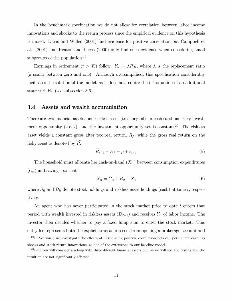
In the benchmark specification we do not allow for correlation between labor income

innovations and shocks to the return process since the empirical evidence on this hypothesis

is mixed. Davis and Willen (2001) find evidence for positive correlation but Campbell et

al. (2001) and Heaton and Lucas (2000) only find such evidence when considering small

subgroups of the population.19

Earnings in retirement (t > K) follow: Yit = λPiK , where λ is the replacement ratio

(a scalar between zero and one). Although oversimplified, this specification considerably

facilitates the solution of the model, as it does not require the introduction of an additional

state variable (see subsection 3.6).

3.4 Assets and wealth accumulation

There are two financial assets, one riskless asset (treasury bills or cash) and one risky invest-

ment opportunity (stock), and the investment opportunity set is constant.20 The riskless

asset yields a constant gross after tax real return, Rf , while the gross real return on the

risky asset is denoted by fR. eRt+1 −Rf = µ+ εt+1 (5)

The household must allocate her cash-on-hand (Xit) between consumption expenditures

(Cit) and savings, so that

Xit = Cit +Bit + Sit (6)

where Sit and Bit denote stock holdings and riskless asset holdings (cash) at time t, respec-

tively.

An agent who has never participated in the stock market prior to date t enters that

period with wealth invested in riskless assets (Bit−1) and receives Yit of labor income. The

investor then decides whether to pay a fixed lump sum to enter the stock market. This

entry fee represents both the explicit transaction cost from opening a brokerage account and19In Section 6 we investigate the effects of introducing positive correlation between permanent earnings

shocks and stock return innovations, as one of the extensions to our baseline model.20Later on will consider a set-up with three diferent financial assets but, as we will see, the results and the

intuition are not significantly affected.

11

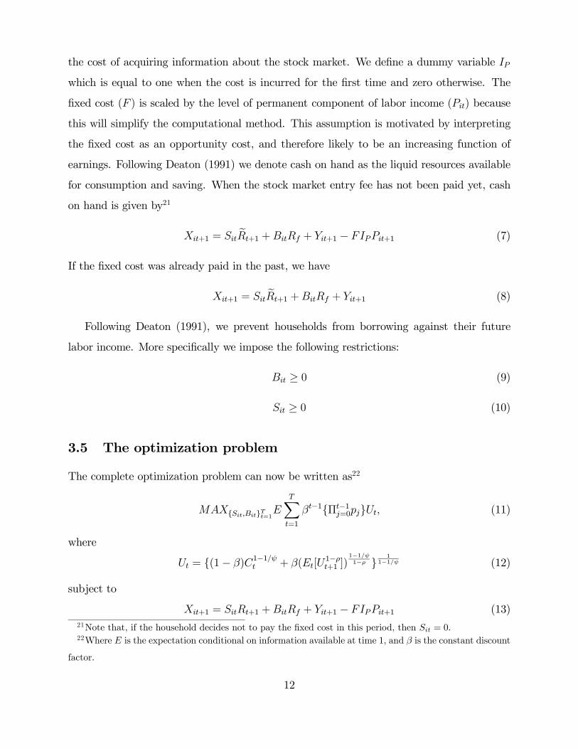
the cost of acquiring information about the stock market. We define a dummy variable IP

which is equal to one when the cost is incurred for the first time and zero otherwise. The

fixed cost (F ) is scaled by the level of permanent component of labor income (Pit) because

this will simplify the computational method. This assumption is motivated by interpreting

the fixed cost as an opportunity cost, and therefore likely to be an increasing function of

earnings. Following Deaton (1991) we denote cash on hand as the liquid resources available

for consumption and saving. When the stock market entry fee has not been paid yet, cash

on hand is given by21

Xit+1 = Sit eRt+1 +BitRf + Yit+1 − FIPPit+1 (7)

If the fixed cost was already paid in the past, we have

Xit+1 = Sit eRt+1 +BitRf + Yit+1 (8)

Following Deaton (1991), we prevent households from borrowing against their future

labor income. More specifically we impose the following restrictions:

Bit ≥ 0 (9)

Sit ≥ 0 (10)

3.5 The optimization problem

The complete optimization problem can now be written as22

MAX{Sit,Bit}Tt=1ETXt=1

βt−1{Πt−1j=0pj}Ut, (11)

where

Ut = {(1− β)C1−1/ψt + β(Et[U

1−ρt+1 ])

1−1/ψ1−ρ } 1

1−1/ψ (12)

subject to

Xit+1 = SitRt+1 +BitRf + Yit+1 − FIPPit+1 (13)21Note that, if the household decides not to pay the fixed cost in this period, then Sit = 0.22Where E is the expectation conditional on information available at time 1, and β is the constant discount

factor.

12

Xit = Sit +Bit + Cit (14)

where IP is a dummy variable that equals one when the household enters the stock market

for the very first time.

Bit ≥ 0 (15)

Sit ≥ 0 (16)

eRt+1 −Rf = µ+ εt+1 (17)

where εt ∼ N(0,σ2ε).If t 6 K

Yit = PitUit (18)

Pit = exp(f(t, Zit))Pit−1Nit (19)

while if t > K

Yit = λPiK (20)

The share of liquid wealth invested in the stock market at age t is denoted by αit.

3.6 Solution Method

Analytical solutions to this problem do not exist. We therefore use a numerical solution

method based on the maximization of the value function to derive optimal policy functions

for total savings and the share of wealth invested in the stock market. The details are given

in appendix A, and here we just present the main idea.

We first simplify the solution by exploiting the scale-independence of the maximization

problem and rewriting all variables as ratios to the permanent component of labor income

(Pit). The equations of motion and the value function can then be rewritten as normalized

variables and we use lower case letters to denote them (for instance, xit ≡ XitPit). This allows

us to reduce the number of state variables to three: age (t), normalized cash-on-hand (xit)

and participation status (whether the fixed cost has already been paid or not). In the last

period the policy functions are trivial (the agent consumes all available wealth) and the

value function corresponds to the indirect utility function. We can use this value function to

13

compute the policy rules for the previous period and given these, obtain the corresponding

value function. This procedure is then iterated backwards. We optimize over the different

choices using grid search.

3.7 Parameter Calibration

We begin by solving the model under a set of “baseline” parameter assumptions at an annual

frequency but we also investigate how our results vary when these parameter values are

changed. For the return process we consider a mean equity premium (µ) equal to 6 percent,

a standard deviation of the risky investment (σε) equal to 18 percent, and a constant real

interest rate (r) of 2 percent. The benchmark preference parameters we use are a coefficient

of relative risk aversion (ρ) equal to 2, an elasticity of intertemporal substitution (ψ) equal to

0.5 and a discount factor (β) equal to 0.95. With these preference parameters the Epstein-

Zin-Weil utility function becomes the standard power utility with a coefficient of relative

risk aversion of 2.

Carroll (1992) estimates the variances of the idiosyncratic shocks using data from the

Panel Study of Income Dynamics, and our baseline simulations use values close to those:

0.1 percent per year for σu and 0.08 percent per year for σn. The deterministic labor

income profile reflects the hump shape of earnings over the life-cycle, and the corresponding

parameter values, just like the retirement transfers (λ), are taken from Cocco, Gomes and

Maenhout (1999).23 It is common practice to estimate different labor income profiles for

different education groups (college graduates, high-school graduates, households without

a high-school degree). For most of the paper we will report the results obtained with the

parameters estimated for the sub-sample of high-school graduates as the results for the other

two groups are very similar. With respect to the fixed cost of participation we consider two

cases; one where the cost is zero and one where it equals 0.1, corresponding to 10% of the

household’s expected annual income.23Cocco, Gomes and Maenhout (1999) report their estimated parameter values and their results are con-

sistent with other studies (for instance, Hubbard, Skinner and Zeldes (1995), Carroll (1997), Gourinchas and

Parker (2001), or Storesletten, Telmer and Yaron (2001)).

14

4 Portfolio Choice and StockMarket Participation over

the Life-Cycle

In this section we discuss the implications of the model with respect to consumption, port-

folio holdings and stock market participation over the life-cycle using computed transition

distributions of cash on hand from one age to the next.

4.1 Computing Transition Distributions

It is common practice for researchers to simulate a model over the life-cycle for a large number

of individuals (say 10000) to compute the statistics of interest (mean wealth holdings, for

instance) for any given age. We propose an alternative method of computing various statistics

that is based on explicitly calculating the transition distribution of cash on hand from one

age to the next.

The numerical details are delegated to Appendix A but the idea is quite simple. Given

that normalized cash on hand is a stationary process, it becomes easy to compute the tran-

sition probability from one cash on hand state to another from period to period once the

optimal policy functions have been computed. Given an initial distribution of cash on hand,

the new distribution will be the product of the transition and initial distribution; this will

then become the initial distribution for the next period.

There are a number of important advantages in using the transition distributions rather

than simulation in this analysis. First, computing the transition distributions is computa-

tionally efficient since it avoids the simulation of a large number of individual life histories.

Second, there is no need to use an interpolation procedure at any stage (see appendix B),

thereby avoiding potential numerical approximation errors that might arise from interpola-

tion. Third, the distributions provide an explicit metric of inequality for different variables

over time and therefore can potentially be more suitable in matching the model to the data.

15

4.2 Results without Fixed Participation Cost

When we consider the case where the fixed participation cost is set equal to zero the results

are similar to the ones previously obtained in this literature.24 Figures 2.1 and 2.2 plot some

of the distributions of normalized cash on hand for different ages during working life and

during retirement, respectively. The distributions can best be thought of as the distributions

of cash on hand that would result if a large number of individuals were born at the same time

(that is, the evolution of the distribution for cash on hand for a particular cohort). Figure 2.1

shows how wealth accumulation affects the distribution of wealth; as wealth accumulation

begins to take place with aging, there is a shift of mean cash on hand to a higher level with

age while at the same time the cash on hand distribution widens.25 Figure 2.2 illustrates

the wealth decumulation that should occur during retirement; mean cash on hand now is

reduced towards mean pensions as the individual ages, while the distribution of cash on hand

is now compressed with age. As the terminal age 100 approaches, the distribution collapses

to a single point (the pension level).

These distributions can now be used to compute the relevant statistics of interest for

the different variables in the model. For instance, mean consumption for this cohort at age

50,denoted by c50, can be computed as26

c50 =JXj=1

π50,j ∗ c(xj, 50) (21)

where c(xj, 50) is the consumption policy rule as a function of the two state variables (nor-

malized cash on hand and age) and π50,j is the probability mass of households aged 50 at

state xj. Using this method, mean normalized consumption and mean normalized wealth are

computed and plotted in Figure 2.3, while Figure 2.4 graphs the mean equity allocation.27

24In this section we only report results using the labor income process estimated for high school graduates.

The results for the other groups are discussed below.25This process continues until retirement when the maximum mean cash on hand is attained. We did not

plot those distributions here to avoid cluttering.26Where J is the number of grid points used in the discretization of normalized cash on hand.27We compute the mean equity allocation across households as total equity holdings divided by total wealth,

and therefore individuals that do not save are automatically excluded. Naturally for these households the

share of wealth in stocks is undefined.

16

The qualitative results are similar to the ones previously obtained in this literature.

Even though earnings risk is uninsurable, labor income is a closer substitute for the risk-

free asset than for equities. As a result, the presence of future labor income against which

the individual cannot borrow, increases the demand for stocks and the share invested in

equities is a decreasing function of cash-on-hand. As the investor approaches retirement,

discounted future labor income is falling and accumulated financial wealth is rising fast.

Therefore the implicit risk-free asset holdings represented by the labor income process become

a less important component of total financial wealth and risk free assets are replenished by

increasing the holdings of the riskless financial asset. Once retired, the household increases

the share of wealth allocated to stocks because labor income uncertainty is eliminated.28

Given our combination of parameter values (less labor income risk and lower prudence)

the typical household accumulates less wealth than in Cocco et. al. (1999) or Campbell

et. al. (2001). As a result, we expect that the investor will allocate a larger fraction of

savings in the risky asset since the optimal share invested in equities is a decreasing function

of cash-on-hand. Furthermore we have a smaller degree of risk aversion and less background

risk which should magnify this portfolio choice effect. Consistent with this intuition, Figure

2.4 identifies a very strong preference for stocks, reflecting the equity premium puzzle from

a portfolio demand perspective.

4.3 Results with Fixed Participation Cost

We next introduce a positive fixed cost of stock market participation. We set this cost equal

to 10% of the household’s expected annual income.

4.3.1 Transition Distributions with the Participation Cost.

Appendix B explains how the initial saving decision generates a distribution for cash on

hand. At the beginning of life (t = 1), the participation rate (defined as the proportion of28See Heaton and Lucas (2000) for the negative effects of background risk on equity investment from a

theoretical and empirical perspective, and Guiso, Japelli and Terlizzese (1996) for further empirical evidence

on the temperance effect of earnings risk on risky asset holdings.

17

households that have incurred the fixed cost at any point in the past) is zero. LetΠOt denote

the mass of agents at each cash on hand state and each age (t), which have not yet paid the

fixed cost yet and therefore are out of the stock market. Given the new distribution for cash

on hand for those out of the market, we can compute the proportion of households who would

be willing to incur the fixed cost; typically, households with high labor income realizations

or high accumulated liquid wealth will find it more beneficial to enter the stock market.

Specifically, the percentage of households that optimally choose to incur the fixed cost and

participate in the stock market can be found by computing the sum of the probabilities

in ΠOt for which x > x∗, where x∗ is the trigger point that causes participation (given by

the optimal participation policy rule). The participation rate can then be computed by

adding to the previous period participation rate, the percentage of households that choose

to pay the fixed cost times the percentage of households who have never paid the cost in the

past. We then compute the distributions for both participants and non-participants, and use

the participation rate to weight each of these distributions in computing the unconditional

distribution of wealth in the economy. Appendix B describes the specific computations in

detail.

4.3.2 Benchmark Case

We first plot the evolution for the distributions of cash on hand for the two types of agents:

participants and non-participants in the stock market. Figure 3.1 illustrates some of the

results by plotting the distributions of normalized cash on hand for individuals aged 30 who

have incurred the fixed cost and those who have not. These are conditional distributions

and the participation rate can be used as a probability weight to generate the unconditional

distribution of cash on hand in the cohort. One recurring feature of the figure is that the

distribution of cash on hand conditional on participation in the stock market has a higher

variance than the wealth distribution for the households which have not participated in the

stock market. Figure 3.2 plots the distributions of cash on hand for ages 50 for both types

of agents. There is now a pronounced spike at around the normalized cash on hand level of

1.42; beyond that level of cash on hand, stock market participation becomes optimal and

18

the two distributions only overlap for a very small interval representing the incurrence of the

fixed entry cost. The distribution is now made up almost completely by rich stockholders

and poor non-stockholders.

Figure 3.3 plots the unconditional mean wealth and consumption over the life-cycle.

The distributions for participants and non-participants are used to compute the respective

means in the two types and then the proportion of stockholders (the participation rate)

is used to take the unconditional average over the two groups. Specifically, let θt denote

the stock market participation rate in the cohort at time (age) t. The unconditional mean

consumption for age t can then be computed as29

ct = θt

(JXj=1

πIt,j ∗ cI(xj, t))+ (1− θt)

(JXj=1

πOt,j ∗ cO(xj, t))

(22)

Figure 3.3 illustrates that the wealth accumulation profile has the same shape as in the

model without the fixed cost (Figure 2.3). In particular, it is useful to note that wealth

accumulation starts to take place at around age 40, and rises quite fast from age 45 onwards,

as households begin to complement their precautionary saving with retirement saving, gen-

erating a substantial wealth accumulation, thus increasing the incentive to enter the stock

market.30

Figure 3.4 plots the unconditional portfolio allocation over the life-cycle31 and the port-

folio allocation conditional on participating in the stock market.32 Even though the share of29Superscript I denotes a variable for households participating in the stock market while superscript O

denotes households out of the stock market.30This is broadly consistent with the results of Cagetti (2001) and Gourinchas and Parker (2001), who

study a model without portfolio choice, and find that saving for retirement takes place at around ages 45−50and 40− 45, respectively.31For a given age t, the unconditional portfolio allocation is computed as:

θt ∗ {PJj=1 π

It,j ∗ αI(xj , t) ∗ (xj − cI(xj , t))}

θt ∗PJ

j=1[πIt,j ∗ (xj − cI(xj , t))] + (1− θt) ∗

PJj=1[π

Ot,j ∗ (xj − cO(xj , t))]

32For a given age t, the portfolio allocation conditional on participation is computed as:

{PJj=1 π

It,j ∗ αI(xj , t) ∗ (xj − cI(xj , t))}

{PJj=1 π

It,j ∗ (xj − cI(xj, t))}

19

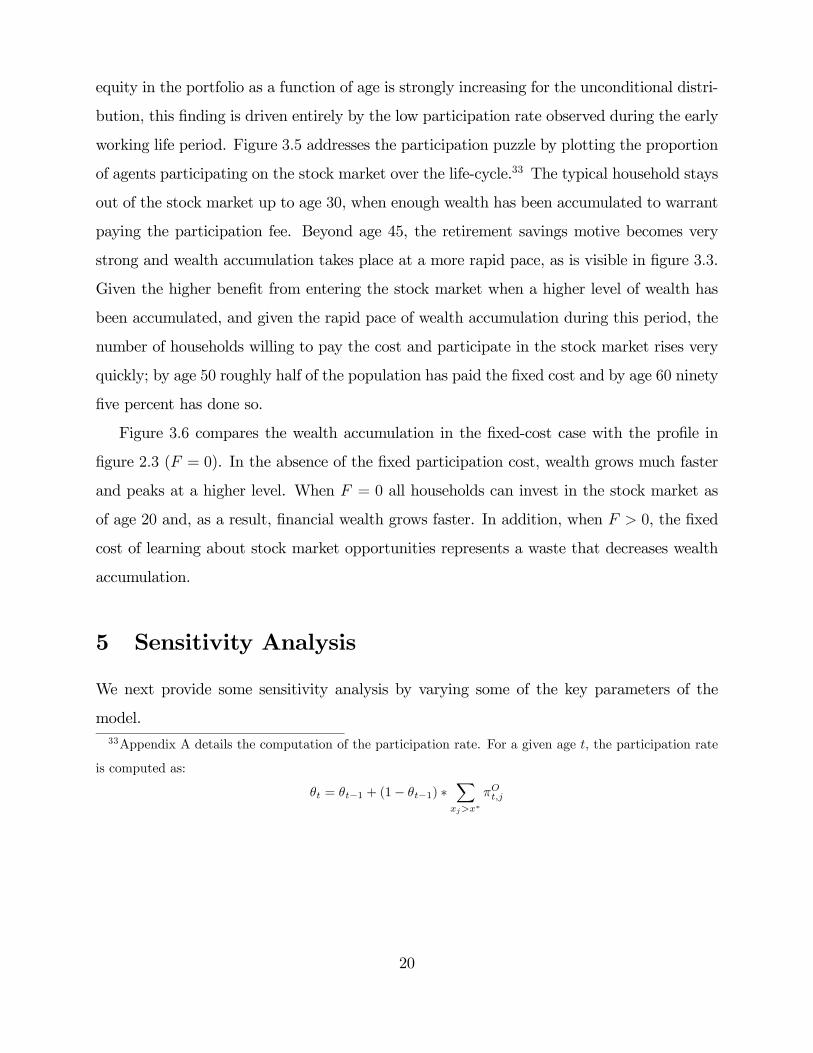
equity in the portfolio as a function of age is strongly increasing for the unconditional distri-

bution, this finding is driven entirely by the low participation rate observed during the early

working life period. Figure 3.5 addresses the participation puzzle by plotting the proportion

of agents participating on the stock market over the life-cycle.33 The typical household stays

out of the stock market up to age 30, when enough wealth has been accumulated to warrant

paying the participation fee. Beyond age 45, the retirement savings motive becomes very

strong and wealth accumulation takes place at a more rapid pace, as is visible in figure 3.3.

Given the higher benefit from entering the stock market when a higher level of wealth has

been accumulated, and given the rapid pace of wealth accumulation during this period, the

number of households willing to pay the cost and participate in the stock market rises very

quickly; by age 50 roughly half of the population has paid the fixed cost and by age 60 ninety

five percent has done so.

Figure 3.6 compares the wealth accumulation in the fixed-cost case with the profile in

figure 2.3 (F = 0). In the absence of the fixed participation cost, wealth grows much faster

and peaks at a higher level. When F = 0 all households can invest in the stock market as

of age 20 and, as a result, financial wealth grows faster. In addition, when F > 0, the fixed

cost of learning about stock market opportunities represents a waste that decreases wealth

accumulation.

5 Sensitivity Analysis

We next provide some sensitivity analysis by varying some of the key parameters of the

model.33Appendix A details the computation of the participation rate. For a given age t, the participation rate

is computed as:

θt = θt−1 + (1− θt−1) ∗Xxj>x∗

πOt,j

20

5.1 Varying Risk Aversion and the Elasticity of Intertemporal

Substitution

5.1.1 CRRA utility function

We start by increasing the coefficient of relative risk aversion (ρ) to 5 while reducing the

elasticity of intertemporal substitution (ψ) to 0.2, thus maintaining the CRRA assumption

(this corresponds to the parameter values used in Campbell et. al. (2001)). A higher ρ

generates both more prudence and more risk aversion. Increasing prudence leads to higher

wealth accumulation over the life-cycle, and consequently increases the demand for stocks

(in levels). On the other hand, higher risk aversion leads to a reduction in the share of

wealth invested in equities. The balance between these effects will, in general, determine the

optimal time at which the fixed entry cost is paid.

Figure 4.1 illustrates that, since wealth accumulation is substantially higher for ρ = 5

than for ρ = 2, the household finds it optimal to enter the stock market at very young ages:

the benefit from utilizing the stock market as a saving vehicle is now higher. As a result,

by age 30, around 50 percent of investors have become participants, while the rate of new

entrants is so fast that by age 35 almost the whole population has entered the stock market

(figure 4.1). The increased rate of stock market participation beyond age 30 is directly

associated with the very fast rate with which wealth accumulation takes place beyond that

age.

Figure 4.2 plots, for comparison purposes, the unconditional share of wealth invested in

the equity market when ρ = 2 and ρ = 5. Given that stock market participation takes place

earlier in life when ρ = 5, the share of wealth in stocks rises beyond that entry point and

there is a complete portfolio allocation to stocks by age 35. As retirement approaches, the

implicit risk free asset in the form of labor income is reduced and there is a shift towards

greater holdings of the riskless asset in the financial portfolio. During retirement, background

labor income risk is eliminated, and the propensity to hold stocks increases.

Figure 4.3 plots the share of wealth invested in stocks conditional on participation. Even

though stronger risk aversion generally reduces the share of wealth invested in equities at

mid-life, the model still predicts excessive stock holding conditional on participation.

21

5.1.2 Non-CRRA utility function

Motivated by the previous results we now deviate from the CRRA framework. By increasing

risk aversion and decreasing the EIS we can reduce the willingness to hold stocks without

increasing saving. Our goal is to increase the coefficient of relative risk aversion above

our benchmark level of ρ = 2, thereby reducing the share of wealth allocated in stocks

due to stronger risk aversion. By simultaneously reducing the elasticity of intertemporal

substitution, we decrease the level of savings (from the weaker motive to smooth consumption

intertemporally), and therefore prevent the participation rate from increasing. It is important

to remember however that with a CRRA utility function, a higher risk aversion coefficient

already implies a low value of the EIS. In particular, for ρ = 5 (ψ = 0.2), we cannot reduce

ψ substantially given that ψ must be non-negative.

Tables 1.1 through 1.4 show, respectively, the mean consumption, mean wealth, mean

portfolio allocation in stocks and the participation rate for different values of ρ and ψ, for

different age groups. Changing ψ has a very small impact on the wealth accumulation of

the young. These households are liquidity constrained, and they only save for precautionary

motives. Consistent with this finding, wealth accumulation increases substantially if we raise

ρ. As a result, ψ has a very small impact on the participation rate which, as seen before, is

an increasing function of ρ. At mid-life, a lower EIS leads to a lower consumption level, as

households want to have a smoother transition to retirement. As a result there is more wealth

accumulation and the portfolio allocation to stocks is reduced. However, as expected, the

improvement is quite marginal and overall the results are very similar to the ones obtained

before.

5.2 Varying the Discount Factor

The previous results show that the participation rate is essentially driven by wealth accumu-

lation. This suggests that if we decrease the discount factor (β) and increase the coefficient of

relative risk aversion, we can simultaneously match participation rates (by reducing wealth

accumulation) and match asset allocation conditional on participation. Figure 4.4 plots the

results of such an attempt. We find that, with a high coefficient of relative risk aversion

22

(ρ = 10), we need a very low discount factor (0.7) to match the participation rates obtained

in the baseline case. Furthermore, the asset allocation conditional on participation is still

extremely high, despite the high coefficient of risk aversion. By reducing wealth accumu-

lation we also reduce the ratio of current financial wealth to future labor income, and this

induces the household to follow a more aggressive investment strategy, offsetting the high

risk aversion effect.

The low discount factor can be viewed as a short-cut representation for tastes shocks such

as housing consumption that requires households to increase their expenditures early in life

and at mid-life. Our results show that such representation does a good job of matching wealth

accumulation and consequently of helping the model to match stock market participation.

However this comes at a cost, as the model’s predictions with respect to asset allocation are

now even more at odds with the data. By reducing financial wealth accumulation over the

life-cycle model we make the portfolio choice puzzles even harder to solve.34

5.3 Other Education Groups

Figure 4.5 shows the participation rate and the mean portfolio allocation when considering

the labor income process of the other two education groups: college graduates and high-

school drop-outs. For the sample of the less educated households (no high-school degree)

stock market participation starts picking up between ages 40 and 50, but it never reaches

100%. The mean allocation to stocks follows a similar pattern and it is actually very close

to 1 from ages 55 through 75. The profiles for college graduates are very similar. For this

group we start the simulation at age 22 since the estimated labor income profile is only valid

from that age onwards. Furthermore, this group has a very steep labor income profile early

in life (see, for example, Cocco et. al. (1999)) and as such they will accumulate less wealth

in the first stage of the life-cycle. Consequently, stock market participation starts later in

life, between ages 45 and 55, but it picks up quite fast.

It is important to remember that the fixed cost in our model is proportional to the level34This is consistent with the results of Cocco (2000). He introduces housing in a life-cycle model of

asset allocation and finds that this improves the model’s ability to match the participation rate. However,

conditional on participation, the model now predicts even larger equity holdings.

23

of income, reflecting an opportunity cost of time devoted to the gathering and processing

of information. However, even though we expect that the absolute value of the opportunity

cost increases with the income level, we also expect that the relative cost will decrease with

the education level. By setting a lower value of F for college graduates and a higher value for

the no high-school group, we would obtain a more intuitive prediction: higher participation

rates for more educated households at every given age. Overall, the results are fairly similar

to the ones obtained in the benchmark case and therefore, for the remainder of the paper,

we will only report results for high-school graduates.

6 Extensions

Our baseline model can match stock-market participation better than previous life-cycle

asset allocation models but, conditional on participation, it still predicts that households

will invest virtually all of their wealth in stocks. Furthermore, it still predicts that all

investors will eventually hold stocks, at some stage of their life. In this section we try to

improve upon these predictions by considering different extensions of the baseline model.35

6.1 Fat Tails in the Distribution of Labor Income Shocks

Empirical evidence suggests that labor income innovations have non-normal distributions.

In particular, earnings are characterized by negative skewness (see, for instance, Chamberlain

and Hirano (1999)). Carroll (1992) estimates that with a probability (p) equal to 0.5 percent,

the transitory labor income shock equals zero (at an annual frequency). The stochastic

process for the innovations to the transitory log labor income shocks is then given by:

ln(Uit) =

ln(U∗it) ∼ N(−0.5σ2u∗,σ2u∗) with probability 1− pη with probability p

(23)

where η is a very small number, and in particular we can consider η = 0. Carroll motivates

this adverse shock as representing layoff risk, but we can also think of it as a reduced form35Given the results in the previous section we will always restrict the analysis to the case of CRRA utility.

Therefore, since we have ψ = 1/ρ, we will refer to the value of ρ.

24

representation a more complicated process, such as the one identified in Chamberlain and

Hirano (1999).

Figures 5.1 and 5.2 plot the life-cycle asset allocation obtained when considering the

specification given by (23), for ρ = 2 and ρ = 5, respectively. For ρ = 2, the co-existence

of cash and stocks in the portfolio begins to be generated, but the magnitude of this effect

is very small. The participation rate also remains close to what is obtained in the baseline

model. Given that the agent is not very risk averse, the effect of dramatically increasing

background labor income risk is negligible. On the other hand, when risk aversion is stronger

(ρ = 5), the possibility of a disastrous labor income shock crowds out stock-holding by a

significant amount. However, the stock market participation rate rises very quickly with age,

implying that the lower participation rates observed in the data cannot be explained by this

alternative specification.

These results suggest that a more detailed calibration of labor income uncertainty is not

likely to improve the performance of the model. If we increase the background risk that

the agent faces, then we can obtain co-existence of cash and stocks in the portfolio, but

we cannot explain non-participation. Risk aversion is driving both results. In the face of a

disastrous labor income shock, albeit transitory, the agent builds up a buffer stock of riskless

asset holdings, generating the co-existence result. However, she also saves more and this

creates a stronger incentive to enter the stock market. Therefore stock market participation

takes place earlier than in the benchmark case. This trade-off was already visible when

we compared the results obtained with different coefficients of risk aversion. These results

are consistent with the ones obtained in sections 5.1 and 5.2, and suggest that any other

extension along the same lines, namely introducing uncertainty about the parameters of the

labor income process, or introducing consumption risk (taste shocks, for instance), is likely

to face the same trade-off.36

36One natural extension along these lines would be to consider explicitly the role of housing consumption

or family-size shocks. Cocco (2000) introduces housing in life-cycle model of asset allocation and finds that

this improves the model’s ability to match the participation rate. However, conditional on participation,

the model now predicts even larger equity holdings. Hu (2001) introduces a renting option in the housing

model, and she requires households to pay a cost if they increase the mortgage size. These two features

generate a positive demand for cash and reduce the demand for equity. However, in her model, there is no

25

6.2 Correlation Between Labor Income Shocks and Stock Returns

The previous results suggest that if we want to improve the empirical performance of the

model, we need to reduce the desirability of owning stocks without, however, simultaneously

increasing the demand for precautionary (or retirement) savings, so as to keep the partici-

pation rate over the life-cycle as in the baseline model. Positive correlation between stock

returns and permanent earnings shocks is a good candidate since it does not affect the con-

sumption policy rule (and therefore does not affect total precautionary saving) but does have

substantial effects on the portfolio allocation between stocks and cash. Moreover, a number

of recent theoretical papers argue for the importance of positive correlation between stock

returns and earnings shocks on portfolio choice.37 Motivated by this literature we extend the

model to allow for positive correlation between permanent labor income shocks and stock

returns.38 More formally, we let the permanent earnings innovation follow:

lnNit = (φεtσε+ (1− φ2)1/2 lnN∗

it)σn (24)

where lnN∗it follows a standard normal, and φ is the correlation coefficient between lnNit

and εtσε.

It should be noted that the existing empirical evidence is mixed. Davis and Willen

stock market entry cost. If such a cost did exist, then naturally, the participation results would be weaker

than the ones obtained in Cocco (2000). Again, the same trade-off between matching participation rates

and asset allocation conditional on participation is obtained.37Viceira (2001), Michaelides (2001), Heaton and Lucas (2000), Campbell, Cocco, Gomes and Maenhout

(2000), Cocco, Gomes and Maenhout (1999), Haliassos and Michaelides (2002) conclude that when stock

returns are positively correlated with labor income shocks, the implied negative hedging demands can be

quite large, thus significantly crowding-out stock holdings, without a first-order impact on the consumption

decision. Large positive correlation between wages and stock returns is also generated endogenously in general

equilibrium models with a Cobb-Douglas production technology (Storesletten, Telmer, Yaron (2001)) and

substantially affects the optimal asset allocation over the life-cycle.38We consider correlation with the permanent labor income shocks as opposed to transitory shocks for

two reasons. First, theory suggests that this correlation should lead to substantial hedging demands (we

have indeed considered correlation between stock returns and transitory labor income shocks, and found

that it has virtually no impact on the optimal asset allocation). Second, this is consistent with the existing

empirical evidence (Davis and Willen (2001)).

26

(2001) estimate significant positive correlations, while Campbell et. al. (2001) and Heaton

and Lucas (2000), obtain mostly small and insignificant values, except for some subgroups

of the population (e.g. self-employed households or households with private businesses).

The results are reported in Figures 6.1 and 6.2.39 For ρ = 5, the negative hedging demand

is substantial and stockholdings are significantly reduced (figure 6.2). Given that total saving

is not affected, the stock market participation decision remains roughly unchanged and all

households participate in the stock market by age 35. However, with a lower risk aversion

coefficient, (ρ = 2), the correlation does not generate a substantial hedging demand since

the agent is not very risk averse (consistent with the results of Viceira (2001)). Therefore,

the stock market participation decision also remains unchanged from the baseline case, and

predicts an upward sloping participation profile over the life-cycle.

We conclude that, even though positive correlation can generate co-existence of cash

and stocks over the life-cycle for higher levels of risk aversion, the stock market participa-

tion decision remains roughly unchanged from the benchmark model for these risk aversion

parameter choices, implying (counterfactually) that all households participate in the stock

market by around age 35.40

6.3 Introducing a third financial asset: long-term bonds

In this section we introduce a third financial asset in model, which we will call (long-term)

bonds. The return process is calibrated to match the historical mean and standard deviation39We set the correlation coefficient (φ) equal to 0.5, a magnitude that we view as an upper bound, given

the empirical evidence.40Another extension along the same lines would be to allow for uncertainty about the structural parameters

of the model. Barberis (2000), Lewellen and Shanken (2000), Pástor (2000) and Kandell and Stambaugh

(1996) among others, have shown how parameter uncertainty can have a strong impact on the optimal

portfolio allocation. The results (not reported here, but available upon request) are virtually the same as

for the positive correlation case. For low values of risk aversion (γ = 2) there is no significant impact.

For moderately high levels of risk aversion (ρ = 5) the co-existence of cash and stocks can be obtained.

Nevertheless, this prediction comes again at the cost of a stock-market participation profile that peaks very

early (by age 40 everyone participates in the stock market).

27

of long-term government bonds in the US:41

eRbt+1 −Rf = µb + εbt+1 (25)

where εbt ∼ N(0,σ2εb), µb = 2%, and σεb = 8%.42

The investor must pay the fixed cost if she wishes to invest in either bonds or stocks.

The motivation is the same as before: the fixed cost represents the direct financial cost and

the opportunity of setting up a broker’s account and “understanding” how the risky assets

work.43

The simulation results are shown in figures 7.1 and 7.2, respectively for ρ = 2 and ρ = 5,

and can be summarized as follows. First, immediately after paying the fixed cost, households

invest almost all of their wealth in stocks. The desire to pay the cost is motivated by the

willingness to hold stocks, not long-term bonds. Second, the participation rate (defined

as the percentage of households that have paid the fixed cost) is virtually the same as in

the 2-asset model. This follows as a natural consequence of the first result. Third, for the

households that have paid the fixed cost, long-term bonds are a substitute for cash, rather

than a substitute for stocks. The share of wealth invested in stocks is not affected by the

presence of this new asset, while cash is replaced by bonds with its share dropping almost

to zero.

These results rationalize the asset allocation puzzle identified by Canner, Mankiw and

Weil (1997): popular financial advisors recommend that more risk-averse investors should

allocate a higher fraction of their risky portfolio (stocks plus bonds) to bonds. This is

inconsistent with the predictions of static and frictionless Capital Asset Pricing Model which

implies that all investors should hold the same combination of risky assets. Their risk aversion41For this calibration we used the returns on 20-year notes as reported by CRSP. The values are not very

sensitive to the choice of the maturity date.42With this specification we abstract from term structure considerations since we are not interested in

market timing issues (see, among others, Campbell, Chan and Viceira (2002), Brennan and Xia (2002),

Campbell and Viceira (2001), or Brennan, Schwartz and Lagnado (1997)).43One could argue that the fixed cost is smaller for government bonds than for stocks and this could

potentially help to improve the predictions of the model. Since the cost is already hard to calibrate, we

decided not to pursue this possibility further at this stage.

28

should only determine the size of their investment to the risky assets as a whole. Our results

show that the presence of undiversifiable human capital rationalizes this puzzle.

Canner et. al. (1997) also restate this puzzle as implying that the ratio of bonds to stocks

should increase when the ratio of stocks to total financial wealth falls. In the context of our

model we do not need heterogeneity in risk aversion to generate this prediction. The ratio

of stocks to total financial wealth falls at mid-life, as the ratio of human capital to financial

wealth falls and the investor is less willing to take risks. The decrease in stock holdings is

compensated by higher bond holdings, thus leading to an increase in the ratio of bonds to

stocks, as recommended by financial consultants.

7 Conclusion

This paper studies optimal consumption and portfolio choice over the life-cycle in the pres-

ence of non-diversifiable idiosyncratic labor income risk, borrowing and short sale constraints

and fixed, one-time, transaction costs associated with stock market participation. We find

that, for plausibly calibrated parameters, stock market participation takes place later in life

typically peaking at around ages 45− 65. Given that surveys usually sample the populationbetween ages 25 and 75, we view this result as moving the model in the right direction for

explaining the median stock-holding puzzle. Moreover, given that entry occurs late in life,

small initial savings is first invested in the riskless asset market and not in the stock market

as the frictionless model would predict.

On the negative side, the model still predicts that all households will have paid the

stock market cost by the time of retirement. Furthermore, conditional on stock market

participation, the share of wealth invested in equities is counterfactually high, generating in

most cases a complete portfolio specialization in stocks. Attempts to generate co-existence of

cash and stocks in the portfolio by increasing the degree of background risk or risk aversion

are moderately successful along that dimension, but fail in generating non-participation,

even very early in working life. Allowing for a (counterfactually) large positive correlation

between stock returns and labor income shocks generates very large riskless asset holdings

only for large values of risk aversion, which are associated with very high participation rates.

29

For low values of risk aversion the impact of the added uncertainty is of second order.

Introducing long-term government bonds in the model, does not alter the basic prediction

of the model that, conditional on stock market participation, households invest almost all

of their wealth in stocks. The desire to pay the fixed cost is driven by willingness to hold

stocks, not long-term bonds; as a result, the participation rate (defined as the percentage

of households which have paid the fixed cost) is virtually the same as in the 2-asset model.

Nevertheless, stock-holders in the 3-asset model, substitute cash with long-term bonds and

increase the share of bond holdings as a fraction of total financial wealth as they age, helping

to rationalize the asset allocation puzzle identified by Canner, Mankiw and Weil (1997).

Overall, the results in this paper suggest that explaining participation rates and asset

allocation simultaneously is still challenging and, in particular, that explanations based solely

on the role of background risk are unlikely to succeed.

30

A Numerical Solution

We first simplify the solution by exploiting the scale-independence of the maximization

problem and rewriting all variables as ratios to the permanent component of labor income

(Pit). The equations of motion and the value function can then be rewritten as normalized

variables and we use lower case letters to denote them (for instance, xit ≡ XitPit). This allows

us to reduce the number of state variables to three; one continuous state variable (cash on

hand) and two discrete state variables (age and participation status). The relevant policy

functions can then be computed as functions of the three state variables: age (t), normalized

cash-on-hand (xit), and participation status (whether the fixed cost has already been paid

or not). In the last period the policy functions are trivial (the agent consumes all available

wealth) and the value function corresponds to the indirect utility function. We can use this

value function to compute the policy rules for the previous period and given these, obtain

the corresponding value function. This procedure is then iterated backwards.

We discretize the state-space (cash-on-hand) and use Gaussian quadrature to approxi-

mate the distributions of the innovations to the labor income process and risky asset returns

(Tauchen and Hussey (1991)). In every period t prior to T , and for each admissible combina-

tion of the state variables, we compute the value associated with each level of consumption,

the decision to pay the fixed cost of entering the stock market, and the share of liquid wealth

invested in stocks. This value is equal to current utility plus the expected discounted con-

tinuation value. To compute this continuation value for points which do not lie on the grid

for the state space we use a univariate cubic spline interpolation procedure along the cash

on hand dimension. The participation decision is obtained by comparing the value functions

for stock market participants (adjusting for the entry cost) and for non-participants. We

optimize over the different choices using grid search.

31

B Computing the Transition Distributions

To find the distribution of cash on hand, we first compute the relevant optimal policy rules;

bond and stock policy functions for stock market participants and non-participants and the

{0, 1} participation rule as a function of cash on hand. Let bI(x) and sI(x) denote thecash and stock policy rules for individuals participating in the stock market respectively and

let bO(x) be the savings decision for the individual out of the stock market. We assume

that households start their working life with zero liquid assets. During working life, for the

households that have not paid the fixed cost, the evolution of normalized cash on hand is

given by44

xt+1 = [bO(xt)Rf ]

½PtPt+1

exp(f(t, Zt))

exp(f(t+ 1, Zt+1))

¾+ Ut+1

= w

µxt| PtPt+1

,exp(f(t, Zt))

exp(f(t+ 1, Zt+1))

¶+ Ut+1

where w(x) is defined by the last equality and is conditional on { PtPt+1

} and the determinis-tically evolving exp(f(t,Zt))

exp(f(t+1,Zt+1)). Denote the transition matrix of moving from xj to xk,45 con-

ditional on being in the bond market as TOkj. Let ∆ denote the distance between the equally

spaced discrete points of cash on hand. The random permanent shock PtPt+1

is discretized

using Gaussian quadrature with m∗ points: PtPt+1

= {Nm}m=m∗m=1 . TOkj = Pr(xt+1=k|xt=j) is

found using46m=m∗Xm=1

Pr

µxt+1|xt, Pt

Pt+1= Nm

¶∗ Pr

µPtPt+1

= Nm

¶(26)

Numerically, this probability is calculated using

TOkjm = Pr

µxk +

∆

2> xt+1 > xk − ∆

2|xt = xj, Pt

Pt+1= Nm

¶Making use the approximation that for small values of σ2u, U ∼ N(exp(µu+ .5∗σ2u), (exp(2∗µu + (σ

2u)) ∗ (exp(σ2u)− 1))), and denoting the mean of U by U and its standard deviation

44To avoid cumbersome notation, the subscript i that denotes a particular individual is omitted in what

follows.45The normalized grid is discretized between (xmin, xmax) where xmin denotes the minimum point on

the equally spaced grid and xmax the maximum point.46The dependence on the determinastically evolving exp(f(t,Zt))

exp(f(t+1,Zt+1))is implied and is omitted from what

follows for expositional clarity.

32

by σ, the transition probability conditional on Nm equals

TOkjm = Φ

Ãxk +

∆2− w(xt|Nm)− U

σ

!− Φ

Ãxk − ∆

2− w(xt|Nm)− U

σ

!

where Φ is the cumulative distribution function for the standard normal. The unconditional

probability from xj to xk is then given by

TOkj =m=m∗Xm=1

TOkjmPr(Nm) (27)

Given the transition matrix TO (letting the number of cash on hand grid points equal to J ,

this is a J by J matrix; TOkj represents the {kth,jth} element), the next period probabilities

of each of the cash on hand states can be found using

πOkt =Xj

TOkj ∗ πOjt−1 (28)

We next use the vector ΠOt (this is a J by 1 vector representing the mass of the population

out of the stock market at each grid point; πOkt represents the {kth} element at time t) and the

participation policy rule to determine the percentage of households that optimally choose

to incur the fixed cost and participate in the stock market. This is found by computing

the sum of the probabilities in ΠOt for which x > x

∗, x∗ being the trigger point that causes

participation (x∗ is determined endogenously through the participation decision rule). These

probabilities are then deleted from ΠOt and are added to Π

It , appropriately renormalizing

both {ΠOt ,Π

It} to sum to one. The participation rate (θt) can be computed at this stage as

θt = θt−1 + (1− θt−1) ∗Xxj>x∗

πOt,j

The same methodology (but with more algebra and computations) can then be used to

derive the transition distribution for cash on hand conditional on being in the stock market

TIt . For stock market participants, the normalized cash on hand evolution equation is

xt+1 = [b(xt)Rf + s(xt) eRt+1]½ PtPt+1

exp(f(t, Zt))

exp(f(t+ 1, Zt+1))

¾+ Ut+1 (29)

= w

µxt| eRt+1, Pt

Pt+1

¶+ Ut+1

33

where w(x) is now conditional on { eRt+1, PtPt+1

}47. The random processes eR and PtPt+1

are

discretized using Gaussian quadrature withm∗ points: R = {Rl}l=m∗l=1 and PtPt+1

= {Nm}m=m∗m=1 .

T Ikj = Pr(xt+1=k|xt=j) is found usingl=m∗Xl=1

m=m∗Xm=1

Pr

µxt+1|xt, eRt+1 = Rl, Pt

Pt+1= Nm

¶∗ Pr( eRt+1 = Rl) ∗ Prµ Pt

Pt+1= Nm

¶(30)

where the independence of PtPt+1

from eRt+1 was used.48 Numerically, this probability is cal-culated using

T Ikjlm = Pr

µxk +

∆

2> xt+1 > xk − ∆

2|xt = xj, Pit

Pit+1= Nm, Rt+1 = Rl

¶The transition probability conditional on Nm and Rl equals

T Ikjlm = Φ

Ãxk +

∆2− w(xt|Nm, Rl)− U

σ

!− Φ

Ãxk − ∆

2− w(xt|Nm, Rl)− U

σ

!

The unconditional probability from xj to xk is then given by

T Ikj =l=10Xl=1

m=10Xm=1

T IkjlmPr(Nm) Pr(Rl) (31)

Given the matrix TI , the probabilities of each of the states are updated by

πIkt+1 =Xj

T Ikj ∗ πIjt (32)

47The dependence on the non-random earnings component is omitted to simplify notation.48The methodology can be applied for an arbitrary correlation structure between the stock market and

permanent shock innovation.

34

References

[1] Abowd, John and David Card. 1989. “On the Covariance Structure of Earnings and

Hours Changes.” Econometrica 57: 411-45.

[2] Aiyagari, Rao, S. and Gertler, Mark. 1991. “Asset Returns With Transactions Costs

and Uninsured Individual Risk.” Journal of Monetary Economics, 27(3), pp. 311-31.

[3] Ameriks, John and Zeldes, Stephen. 2001. “How Do Household Portfolio Shares Vary

With Age?” Working Paper, Columbia Business School.

[4] Attanasio, Orazio; Banks, James; and Tanner, Sarah. 2002. “Asset Holding and Con-

sumption Volatility” Journal of Political Economy, forthcoming.

[5] Barberis, Nicholas. 2000. “Investing for the Long-Run when Returns are Predictable.”

Journal of Finance 55, 225-264.

[6] Basak, Suleyman and Cuoco, Domenico. 1998. “An Equilibrium Model with Restricted

Stock Market Participation.” Review of Financial Studies, 11(2), pp. 309-41.

[7] Bertaut, C. and Michael Haliassos. 1997. “Precautionary Portfolio Behavior from a

Life-Cycle Perspective.” Journal of Economic Dynamics and Control, 21, 1511-1542.

[8] Brav, Alon, Constantinides, George M. and Geczy, Christopher C. 2002. “Asset Pric-

ing with Heterogeneous Consumers and Limited Participation: Empirical Evidence.”

Journal of Political Economy, forthcoming.

[9] Brennan, Michael and Yihong Xia, 2002, “Dynamic Asset Allocation Under Inflation.”

Journal of Finance, forthcoming.

[10] Brennan, Michael and Yihong Xia, 2000, “Stochastic Interest Rates and Bond-Stock

Mix.” European Finance Review, 4, 197-210.

[11] Brennan, M., E. Schwartz and R. Lagnado. 1997. “Strategic Asset Allocation.” Journal

of Economic Dynamics and Control 21, 1377-1403.

35

[12] Cagetti, Marco. 2001. “Wealth Accumulation over the life cycle and Precautionary Sav-

ings” UVA working paper.

[13] Campbell, John, Y. Lewis Chan and Luis Viceira. 2002. “A Multivariate Model of

Strategic Asset Allocation.” Journal of Financial Economics, forthcoming.

[14] Campbell, John, Joao Cocco, Francisco Gomes and Pascal Maenhout. 2001. “Investing

Retirement Wealth: A Life-Cycle Model.” In “Risk Aspects of Social Security Reform.”

University of Chicago Press.

[15] Campbell, John and Luis Viceira. 2001 “Who Should Buy Long-Term Bonds?” Amer-

ican Economic Review, 91, 99-127.

[16] Canner, Niko, N. Gregory Mankiw and David N. Weil, “An Asset Allocation Puzzle,”

American Economic Review, 1997, 87, 181-191.

[17] Carroll, Christopher D.. 1992. “The Buffer-Stock Theory of Saving: Some Macroeco-

nomic Evidence.” Brookings Papers on Economic Activity no. 2: 61-156.

[18] Carroll, Christopher D.. 1997. “Buffer Stock Saving and the Life-Cycle / Permanent

Income Hypothesis.” Quarterly Journal of Economics CXII no. 1: 3-55.

[19] Carroll, Christopher and Andrew Samwick. 1997. “The Nature of Precautionary

Wealth.” Journal of Monetary Economics, 40(1).

[20] Chamberlain, G. and K. Hirano. 1999. “Predictive Distributions Based on Longitudinal

Earnings Data.” Annals of Economics and Statistics Sep-Dec, 211-242.

[21] Cocco, Joao. 2000. “Portfolio Choice in the Presence of Housing.” Working Paper.

London Business School.

[22] Cocco, J., F. Gomes and P. Maenhout. 1999. “Portfolio Choice Over The Life-Cycle.”

Working Paper. Harvard University.

[23] Constantinides, George. 1986. “Capital Market Equilibrium with Transaction Costs.”

Journal of Political Economy; 94, pages 842-62.

36

[24] Constantinides, George, Donaldson John and Mehra Rajnish. 2001. “Junior Can’t Bor-

row: A New Perspective on the Equity Premium Puzzle.” Quarterly Journal of Eco-

nomics.

[25] Dammon, Robert, Chester Spatt and Harold Zhang. 2001. “Optimal Consumption and

Investment with Capital Tax Gains” Review of Financial Studies, forthcoming.

[26] Davis, S. and P. Willen. 2001. “Occupation-level Income Shocks and Asset Returns:

Their Covariance and Implications for Portfolio Choice.” Working Paper, University of

Chicago.

[27] Deaton, Angus. 1991. “Saving and Liquidity Constraints.” Econometrica 59(5): 1221-

48.

[28] Degeorge, Francois, Dirk Jenter, Alberto Moel and Peter Tufano. 2002. “Selling Com-

pany Shares to Reluctant Employees: France Telecom’s Experience.” Working Paper,

HEC and Harvard University.

[29] Epstein, Lawrence and Stanley Zin. 1989. “Substitution, Risk Aversion, and the Tempo-

ral Behavior of Consumption and Asset Returns: A Theorethical Framework.” Econo-

metrica, 57, 937-969.

[30] Gakidis, Haralabos. 1998. “Stocks for the Old? Earnings Uncertainty and Life-Cycle

Portfolio Choice.” MIT doctoral thesis.

[31] Gourinchas Pierre-Olivier and Jonathan Parker. 2001. “Consumption over the Life-

Cycle.” Econometrica, forthcoming.

[32] Guiso, Luigi, Tullio Jappelli and Daniele Terlizzese. 1996. “Income Risk, Borrowing

Constraints and Portfolio Choice.” American Economic Review vol. 86, pp. 158-172.

[33] Guiso, Luigi, Michael Haliassos and Tullio Japelli. 2001. “Household Portfolios: An

International Comparison.” in Household Portfolios, eds. Luigi Guiso, Michael Haliassos

and Tullio Japelli, MIT Press.

37

[34] Haliassos, Michael and Alexander Michaelides. 2002. “Portfolio Choice and Liquidity

Constraints.” International Economic Review, forthcoming.

[35] He, Hua and Modest, David, M. 1995. “Market Frictions and Consumption-Based Asset

Pricing.” Journal of Political Economy, 103(1), pp. 94-117.

[36] Heaton John, and Deborah Lucas. 1996. “Evaluating the Effects of Incomplete Markets

on Risk Sharing and Asset Pricing.” Journal of Political Economy, 104(3), pp. 443-87.

[37] Heaton John, and Deborah Lucas. 1997. “Market Frictions, Savings Behavior, and Port-

folio Choice.” Macroeconomic Dynamics, 1(1): 76-101.

[38] Heaton John, and Deborah Lucas. 2000. “Portfolio Choice and Asset Prices: The Im-

portance of Entrepreneurial Risk.” Journal of Finance, 55: 1163-1198.

[39] Hong, Harrison, Jeffrey Kubik, and Jeremy Stein. 2001. “Social Interaction and Stock

Market Participation.” Working Paper, Stanford University, Syracuse University and

Harvard University.

[40] Hochguertel, Stefan. 1999. “A Buffer-Stock Model with Portfolio Choice: Implications

of Income Risk and Liquidity Constraints.” Working-Paper, Tilburg University.

[41] Hu, Xiaoqing. 2001. “Portfolio Choices for Home Owners.” Working Paper. Northwest-

ern University.

[42] Hubbard, Glenn, Jonathan Skinner, and Stephen Zeldes. 1995. “Precautionary Saving

and Social Insurance.” Journal of Political Economy, 103: 360-399.

[43] Jagannathan, R. and N. R. Kocherlakota. 1996. “Why Should Older People Invest Less

in Stocks Than Younger People?” Federal Reserve Bank of Minneapolis, Quarterly

Review, 11-23.

[44] Kandel, S. and Stambaugh, R. F. 1996. “On the Predictability of Stock Returns: An

Asset Allocation Perspective.” Journal of Finance, 51, 385-424.

38

[45] Koo, H. K. 1998. “Consumption and Portfolio Selection with Labor Income: A Contin-

uous Time Approach.” Mathematical Finance, 8, 49-65.

[46] King, Mervyn and Jonathan Leape. 1998. “Wealth and Portfolio Composition: Theory

and Evidence.” Journal of Public Economics, 69, 155-193.

[47] Lewellen, Jonathan and Jay Shanken. 2000. “Estimation Risk, Market Efficiency and

the Predictability of Returns.” Working Paper, M.I.T. and University of Rochester.

[48] Lucas, Deborah. 1994. “Asset Pricing with Undiversifiable Risk and Short Sales Con-

straints: Deepening the Equity Premium Puzzle”, Journal of Monetary Economics, 34,

325-41.

[49] Ludvigson, Sydney and Alexander Michaelides. 2001. “Does Buffer Stock Saving Explain

the Smoothness and Excess Sensitivity of Conumption?” American Economic Review,

91(3), pp. 631-647.

[50] Luttmer, Erzo, G, J. 1996. “Asset Pricing in Economies with Frictions.” Econometrica,

64(6), pp. 1439-67.

[51] Luttmer, Erzo, G, J. 1999. “What Level of Fixed Costs Can Reconcile Consumption

and Stock Returns?” Journal of Political Economy, 107(5), pp. 969-97.

[52] MaCurdy, T. E.. 1981. “The use of time series processes to model the error structure of

earnings in longitudinal data analysis.” Journal of Econometrics, 18: 83-114.

[53] Malkiel, G., Burton. 1999. “A RandomWalk DownWall Street.” 7th edition, New York:

Norton.

[54] Mankiw, N. Gregory and Stephen Zeldes. 1991. “The Consumption of Stockholders and

Non-Stockholders.” Journal of Financial Economics, 29, 97-112.

[55] Merton, Robert C. 1971. “Optimum Consumption and Portfolio Rules in a Continuous-

Time Model.” Journal of Economic Theory, 3, 373-413.

39

[56] Michaelides, Alexander. 2001. “Portfolio Choice, Liquidity Constraints and Stock Mar-

ket Mean Reversion.” CEPR Discussion Paper No. 2823.

[57] Paiella, Monica. 2000. “Transaction Costs and Limited Stock Market Participation to

Reconcile Asset Prices and Consumption Choices.” Working Paper.

[58] Pástor, ,Luboš. 2000. “Portfolio Selection and Asset Pricing Models.” Journal of Finance

55, 179-223.

[59] Pischke Jörn-Steffen. 1995. “Individual Income, Incomplete Information and Aggregate

Consumption,” Econometrica. Vol.63, No.4, 805-840.

[60] Polkovnichenko, Valery. 2000. “Heterogeneous Labor Income and Preferences: Implica-

tions for Stock Market Participation.” University of Minnesota Working Paper.

[61] Poterba, James and Andrew Samwick. 1999. “Household Portfolio Allocation over the

Life-Cycle.” NBER Working Paper 6185.

[62] Samuelson, P. A. 1969. “Lifetime Portfolio Selection by Dynamic Stochastic Program-

ming.” Review of Economics and Statistics, 51, 239-46.

[63] Storesletten, Kjetil, Telmer Chris and Yaron Amir. 2001. “Persistent Idiosyncratic

Shocks and Incomplete Markets.” Working paper, Carnegie Mellon University, Stock-

holm School of Economics and The Wharton School.

[64] Tauchen, G. and R. Hussey. 1991. “Quadrature-Based Methods for Obtaining Approx-

imate Solutions to Nonlinear Asset Pricing Models.” Econometrica, 59, 371-396.

[65] Telmer, Chris . 1993. “Asset-Pricing Puzzles and Incomplete Markets.” Journal of Fi-

nance, 48, 1803-32.

[66] Vayanos. Dimitri. 1998. “Transaction Costs and Asset Prices: A Dynamic Equilibrium

Model.” Review of Financial Studies, 11(1), pp. 1-58.

[67] Viceira, Luis. 2001. “Optimal Portfolio Choice for Long-Horizon Investors with Non-

tradable Labor Income.” Journal of Finance, 55, 1163-98.

40

[68] Vissing-Jorgensen, Annette. 2002. “Limited Asset Market Participation and the Elas-

ticity of Intertemporal Substitution.” Journal of Political Economy, Forthcoming.

[69] Weil, Phillipe. 1989. “The Equity Premium Puzzle and the Risk-Free Rate Puzzle.”

Journal of Monetary Economics, 24, 401-421.

41

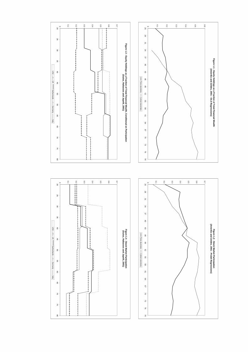
Figure 1.1 - Equity Holdings as a Fraction of Total Financial W

ealth(A

meriks and Zeldes, 2001 - O

LS Regressions)

0

0.1

0.2

0.3

0.4

0.5

0.6

2528

3134

3740

4346

4952

5558

6164

6770

7376

79

Time dum

mies

Cohort dum

mies

Figure 1.2 - Stock Market Participation

(Am

eriks and Zeldes, 2001 - Probit Regressions)

0

0.1

0.2

0.3

0.4

0.5

0.6

0.7

2528

3134

3740

4346

4952

5558

6164

6770

7376

79

Time dum

mies

Cohort dum

mies

Figure 1.3 - Equity Holdings as a Fraction of Total Financial W

ealth, Conditional on Participation

(Guiso, H

aliassos and Japelli, 2001)

0

0.1

0.2

0.3

0.4

0.5

0.6

0.7

2025

3035

4045

5055

6065

7075

80

USA

UK

Netherlands

Germ

anyItaly

Figure 1.4 - Stock Market Participation

(Guiso, H

aliassos and Japelli, 2001)

0

0.1

0.2

0.3

0.4

0.5

0.6

0.7

2025

3035

4045

5055

6065

7075

80

USA

UK

Netherlands

Germ

anyItaly

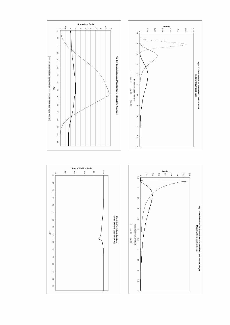
Fig 2.1: Distributions for N

ormalized C

ash on Hand

Model w

ithout fixed cost

0

0.02

0.04

0.06

0.08

0.1

0.12

0.140.51

1.52

2.53

3.54

4.55

5.56

Norm

alized Cash on H

and

Density

Age 25Age 35

Age 45

Fig 2.2: Distributions for N

ormalized C

ash on Hand (R

etirement stage)

Model w

ithout the fixed cost

0

0.01

0.02

0.03

0.04

0.05

0.06

0.07

0.080.51

1.52

2.53

3.54

4.55

5.56

Norm

alized Cash on H

and

Density

Age 80Age 75

Fig. 2.4: Portfolio Allocation

Model W

ithout the Fixed Cost

0%

20%

40%

60%

80%

100%

2227

3237

4247

5257

6267

7277

8287

9297

Age

Share of Wealth in Stocks

Fig. 2.3: Consum

ption and Wealth M

odel without the fixed cost

0

0.5 1

1.5 2

2.5 3

3.5 4

4.5 5

2227

3237

4247

5257

6267

7277

8287

9297

Age

Normalized Cash

Mean N

ormalized consum

ptionM

ean normalized liquid w

ealth

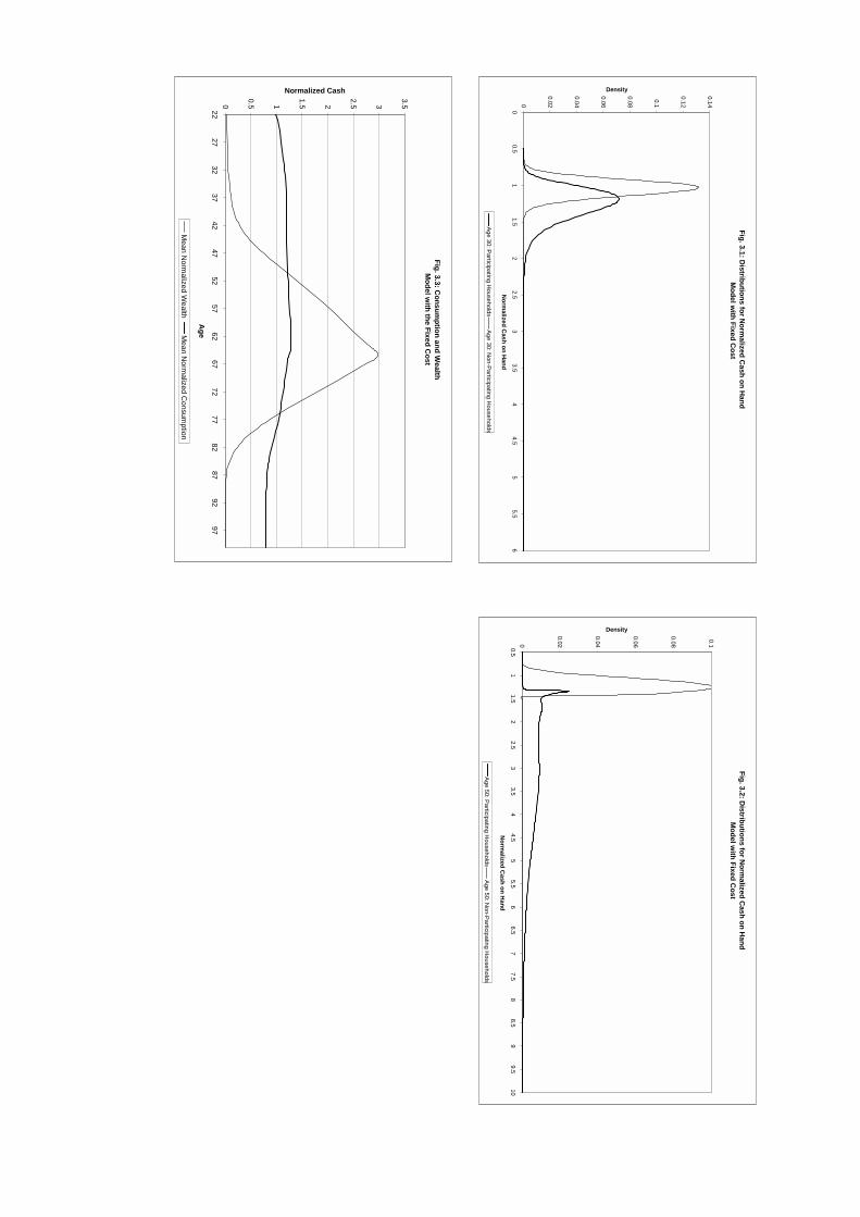
Fig. 3.1: Distributions for N

ormalized C

ash on Hand

Model w

ith Fixed Cost

0

0.02

0.04

0.06

0.08

0.1

0.12

0.14

00.5

11.5

22.5

33.5

44.5

55.5

6

Norm

alized Cash on H

and

Density

Age 30: Participating Households

Age 30: Non-Participating H

ouseholds

Fig. 3.2: Distributions for N

ormalized C

ash on Hand

Model w

ith Fixed Cost

0

0.02

0.04

0.06

0.08

0.10.51

1.52

2.53

3.54

4.55

5.56

6.57

7.58

8.59

9.510

Norm

alized Cash on H

and

Density

Age 50: Participating Households

Age 50: Non-Participating H

ouseholds

Fig. 3.3: Consum

ption and Wealth

Model w

ith the Fixed Cost

0

0.5 1

1.5 2

2.5 3

3.5

2227

3237

4247

5257

6267

7277

8287

9297

Age

Normalized Cash

Mean N

ormalized W

ealthM

ean Norm

alized Consum

ption

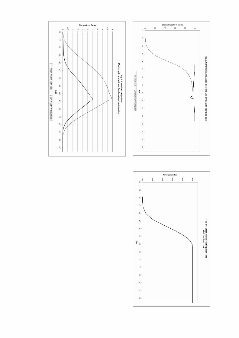
Fig. 3.5: Stock Market Participation R

ateW

ith the fixed cost

0%

20%

40%

60%

80%

100%

2227

3237

4247

5257

6267

7277

8287

9297

Age

Participation Rate

Fig. 3.4: Portfolio Allocation over the Life-C

ycle with the fixed cost

0

0.2

0.4

0.6

0.8 1

2227

3237

4247

5257

6267

7277

8287

9297

Age

Share of Wealth in Stocks

Unconditional

Conditional on Participation

Fig 3.6: Wealth C

omparison

Models w

ith and without fixed costs of participation

0

0.5 1

1.5 2

2.5 3

3.5 4

4.5 5

2227

3237

4247

5257

6267

7277

8287

9297

Age

Normalized Cash

Mean W

ealth (with cost)

Mean W

ealth Without C

ost

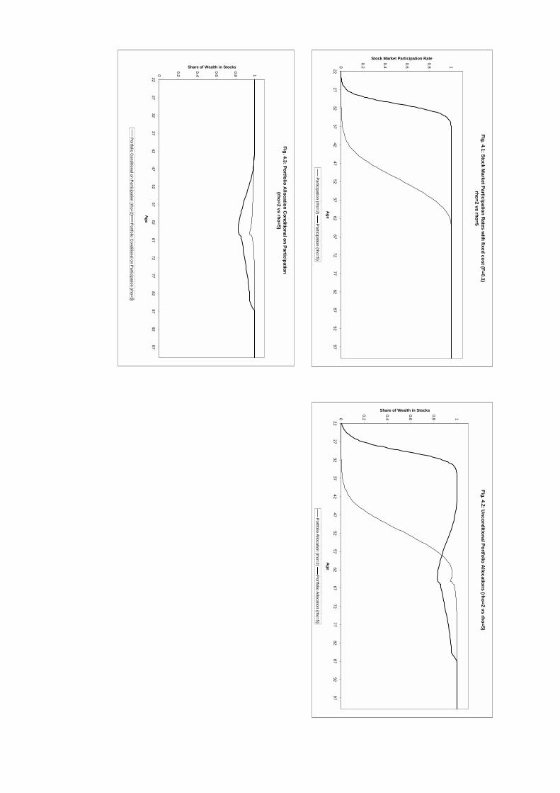
Fig. 4.1: Stock Market Participation R

ates with fixed cost (F=0.1)

rho=2 vs rho=5

0

0.2

0.4

0.6

0.8 1

2227

3237

4247

5257

6267

7277

8287

9297

Age

Stock Market Participation Rate

Participation (rho=2)Participation (rho=5)

Fig. 4.2: Unconditional Portfolio A

llocations (rho=2 vs rho=5)

0

0.2

0.4

0.6

0.8 1

2227

3237

4247

5257

6267

7277

8287

9297

Age

Share of Wealth in Stocks

Portfolio Allocation (rho=2)Portfolio Allocation (rho=5)

Fig. 4.3: Portfolio Allocation C

onditional on Participation (rho=2 vs rho=5)

0

0.2

0.4

0.6

0.8 1

2227

3237

4247

5257

6267

7277

8287

9297

Age

Share of Wealth in Stocks

Portfolio Conditional on Participation (rho=2)

Portfolio Conditional on Participation (rho=5)

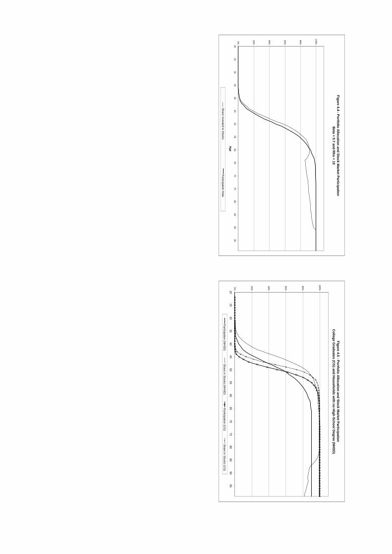
Figure 4.4 - Portfolio Allocation and Stock M

arket Participation B

eta = 0.7 and Rho = 10

0%

20%

40%

60%

80%

100%

2025

3035

4045

5055

6065

7075

8085

9095

Age

Share Invested in StocksParticipation R

ate

Figure 4.5 - Portfolio Allocation and Stock M

arket ParticipationC

ollege Graduates (C

G) and H

ouseholds with no H

igh-School Degree (N

HSD

)

0%

20%

40%

60%

80%

100%

2025

3035

4045

5055

6065

7075

8085

9095

Participation (NH

SD)

Share in Stocks (NH

SD)

Participation (CG

)Share in Stocks (C

G)

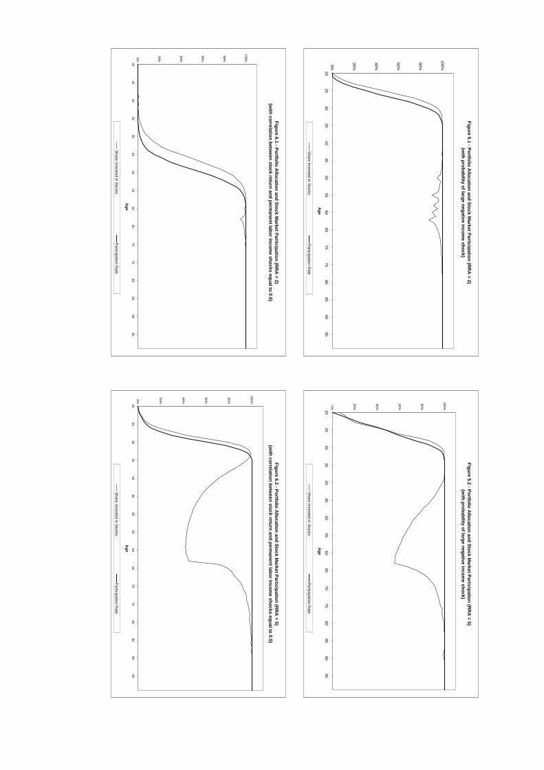
Figure 5.1 - Portfolio Allocation and Stock M

arket Participation (RR

A = 2)

(with probability of large negative incom

e shock)

0%

20%

40%

60%

80%

100%

2025

3035

4045

5055

6065

7075

8085

9095

Age

Share Invested in StocksParticipation R

ate

Figure 5.2 - Portfolio Allocation and Stock M

arket Participation (RR

A = 5)

(with probability of large negative incom

e shock)

0%

20%

40%

60%

80%

100%

2025

3035

4045

5055

6065

7075

8085

9095

Age

Share Invested in StocksParticipation R

ate

Figure 6.1 - Portfolio Allocation and Stock M

arket Participation (RR

A = 2)

(with correlation betw

een stock return and permanent labor incom

e shocks equal to 0.5)

0%

20%

40%

60%

80%

100%

2025

3035

4045

5055

6065

7075

8085

9095

Age

Share Invested in StocksParticipation R

ate

Figure 6.2 - Portfolio Allocation and Stock M

arket Participation (RR

A = 5)

(with correlation betw

een stock return and permanent labor incom

e shocks equal to 0.5)

0%

20%

40%

60%

80%

100%

2025

3035

4045

5055

6065

7075

8085

9095

Age

Share Invested in StocksParticipation R

ate

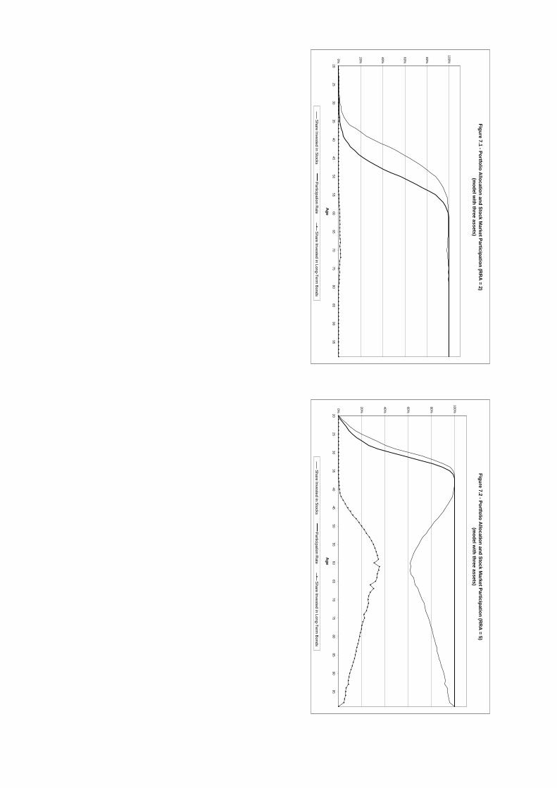
Figure 7.2 - Portfolio Allocation and Stock M

arket Participation (RR

A = 5)

(model w

ith three assets)

0%

20%

40%

60%

80%

100%

2025

3035

4045

5055

6065

7075

8085

9095

Age

Share Invested in StocksParticipation R

ateShare Invested in Long-Term

Bonds

Figure 7.1 - Portfolio Allocation and Stock M

arket Participation (RR

A = 2)

(model w

ith three assets)

0%

20%

40%

60%

80%

100%

2025

3035

4045

5055

6065

7075

8085

9095

Age

Share Invested in StocksParticipation R

ateShare Invested in Long-Term

Bonds

Table 1.1 - Mean Normalized Consumption for different age groups.

Results are shown for different values of the elasticity of intertemporal

substitution (in columns), and different values of the coefficient of relative

risk aversion (in rows).

Ages 20 to 350.75 0.5 0.25 0.1

4/3 1.401 1.402 1.399 1.4002 1.365 1.399 1.397 1.3924 1.287 1.735 1.725 1.339

10 1.237 1.249 1.251 1.227

Ages 36 to 500.75 0.5 0.25 0.1

4/3 1.775 1.782 1.785 1.7862 1.675 1.697 1.733 1.7464 1.835 2.069 1.999 1.726

10 1.912 1.984 1.899 1.766

Ages 51 to 650.75 0.5 0.25 0.1

4/3 1.566 1.619 1.627 1.6292 1.991 1.699 1.662 1.6654 2.167 1.921 1.879 1.944

10 2.175 2.159 2.143 1.962

Ages 66 to 800.75 0.5 0.25 0.1

4/3 1.163 1.036 1.029 1.0262 1.873 1.539 1.285 1.1844 1.959 1.213 1.255 1.839

10 1.849 1.668 1.781 1.880

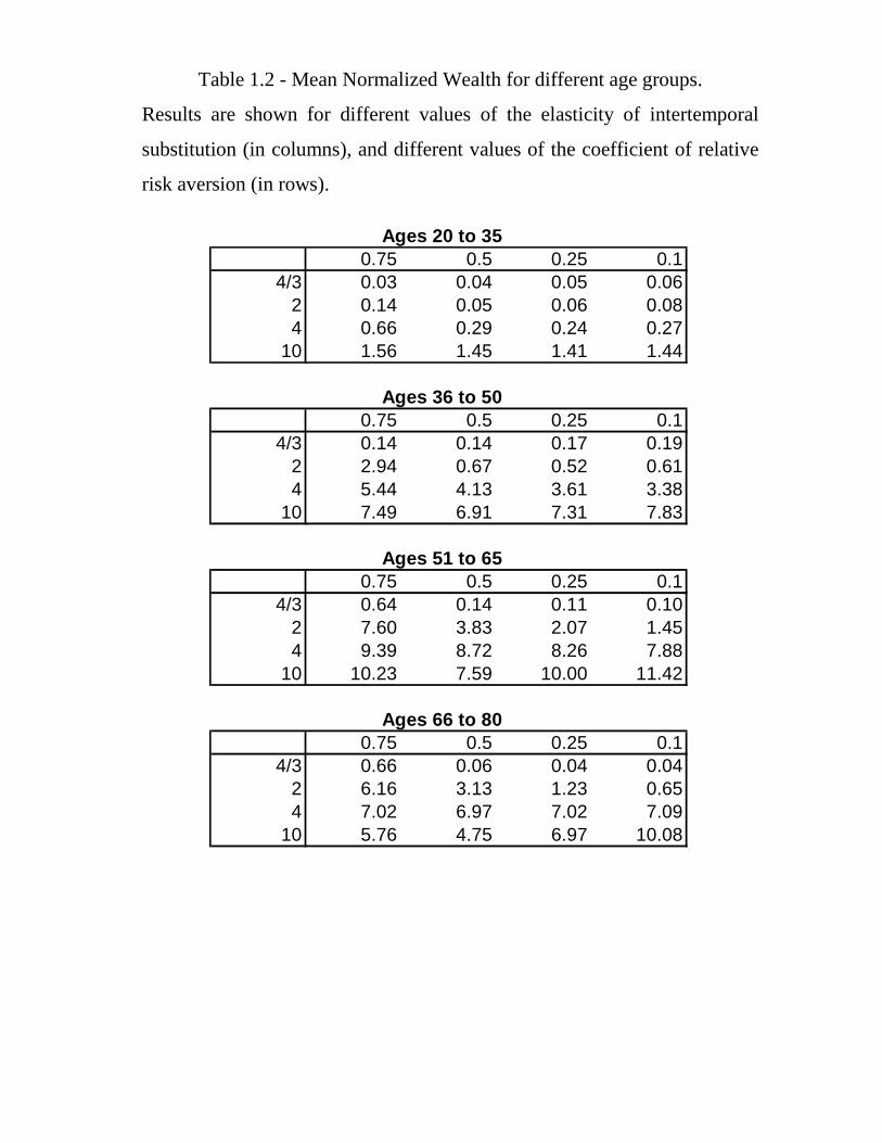
Table 1.2 - Mean Normalized Wealth for different age groups.

Results are shown for different values of the elasticity of intertemporal

substitution (in columns), and different values of the coefficient of relative

risk aversion (in rows).

Ages 20 to 350.75 0.5 0.25 0.1

4/3 0.03 0.04 0.05 0.062 0.14 0.05 0.06 0.084 0.66 0.29 0.24 0.27

10 1.56 1.45 1.41 1.44

Ages 36 to 500.75 0.5 0.25 0.1

4/3 0.14 0.14 0.17 0.192 2.94 0.67 0.52 0.614 5.44 4.13 3.61 3.38

10 7.49 6.91 7.31 7.83

Ages 51 to 650.75 0.5 0.25 0.1

4/3 0.64 0.14 0.11 0.102 7.60 3.83 2.07 1.454 9.39 8.72 8.26 7.88

10 10.23 7.59 10.00 11.42

Ages 66 to 800.75 0.5 0.25 0.1

4/3 0.66 0.06 0.04 0.042 6.16 3.13 1.23 0.654 7.02 6.97 7.02 7.09

10 5.76 4.75 6.97 10.08

Table 1.3 - Mean Share of Wealth Invested in Stocks for different age groups.

Results are shown for different values of the elasticity of intertemporal

substitution (in columns), and different values of the coefficient of relative

risk aversion (in rows).

Ages 20 to 350.75 0.5 0.25 0.1

4/3 0% 0% 0% 0%2 51% 4% 0% 0%4 78% 55% 31% 38%

10 77% 76% 77% 76%

Ages 36 to 500.75 0.5 0.25 0.1

4/3 14% 0% 0% 0%2 99% 60% 29% 24%4 100% 100% 99% 99%

10 80% 92% 87% 54%

Ages 51 to 650.75 0.5 0.25 0.1

4/3 58% 0% 0% 0%2 97% 99% 95% 87%4 92% 92% 90% 85%

10 56% 70% 52% 33%

Ages 66 to 800.75 0.5 0.25 0.1

4/3 98% 0% 0% 0%2 99% 100% 100% 100%4 97% 95% 94% 91%

10 73% 78% 67% 57%

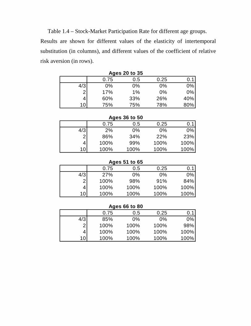
Table 1.4 – Stock-Market Participation Rate for different age groups.

Results are shown for different values of the elasticity of intertemporal

substitution (in columns), and different values of the coefficient of relative

risk aversion (in rows).

Ages 20 to 350.75 0.5 0.25 0.1

4/3 0% 0% 0% 0%2 17% 1% 0% 0%4 60% 33% 26% 40%

10 75% 75% 78% 80%

Ages 36 to 500.75 0.5 0.25 0.1

4/3 2% 0% 0% 0%2 86% 34% 22% 23%4 100% 99% 100% 100%

10 100% 100% 100% 100%

Ages 51 to 650.75 0.5 0.25 0.1

4/3 27% 0% 0% 0%2 100% 98% 91% 84%4 100% 100% 100% 100%

10 100% 100% 100% 100%

Ages 66 to 800.75 0.5 0.25 0.1

4/3 85% 0% 0% 0%2 100% 100% 100% 98%4 100% 100% 100% 100%

10 100% 100% 100% 100%