Embed Size (px)
Citation preview
Pore-Scale Model for Rate Dependence of Two-Phase Flow in Porous Media
Mohammed Al-Gharbi
Supervisor: Prof. Martin Blunt
Presentation outline
• Why rate-dependent effects are important
• Methodology for rate-dependent modelling
• Project structure
• Future development of the model
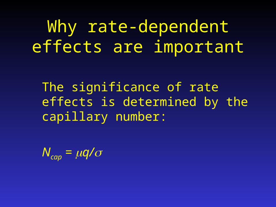
Why rate-dependent effects are important
The significance of rate effects is determined by the capillary number:
Ncap = q/
Why rate-dependent effects are important
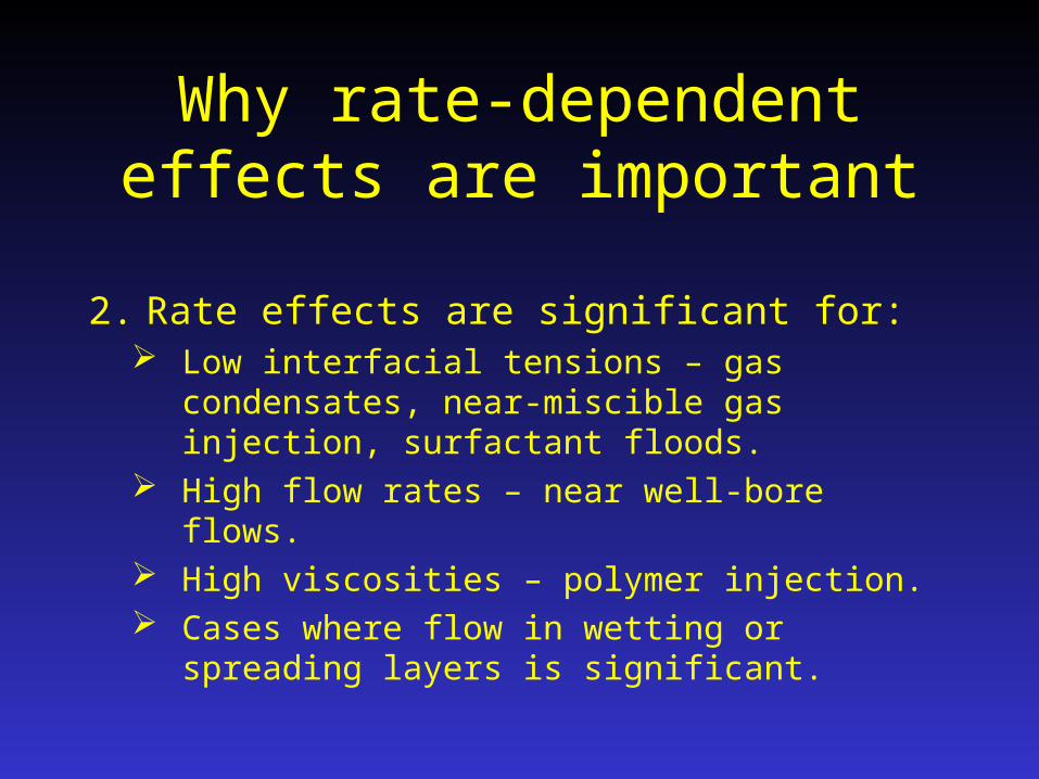
2. Rate effects are significant for: Low interfacial tensions – gas condensates,
near-miscible gas injection, surfactant floods. High flow rates – near well-bore flows. High viscosities – polymer injection. Cases where flow in wetting or spreading
layers is significant.

Why rate-dependent effects are important
1. Lab exp.: Richardson (1952) Aim: Effect of displacement rate on residual
saturation. Result: Less trapping as flow rate increases. Deduction: Rel.perm. & residual So = f(Qinj).
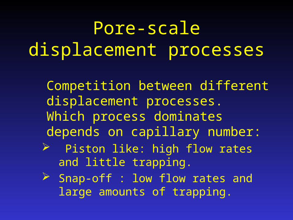
Pore-scale displacement processes
Competition between different displacement processes. Which process dominates depends on capillary number:
Piston like: high flow rates and little trapping.
Snap-off : low flow rates and large amounts of trapping.
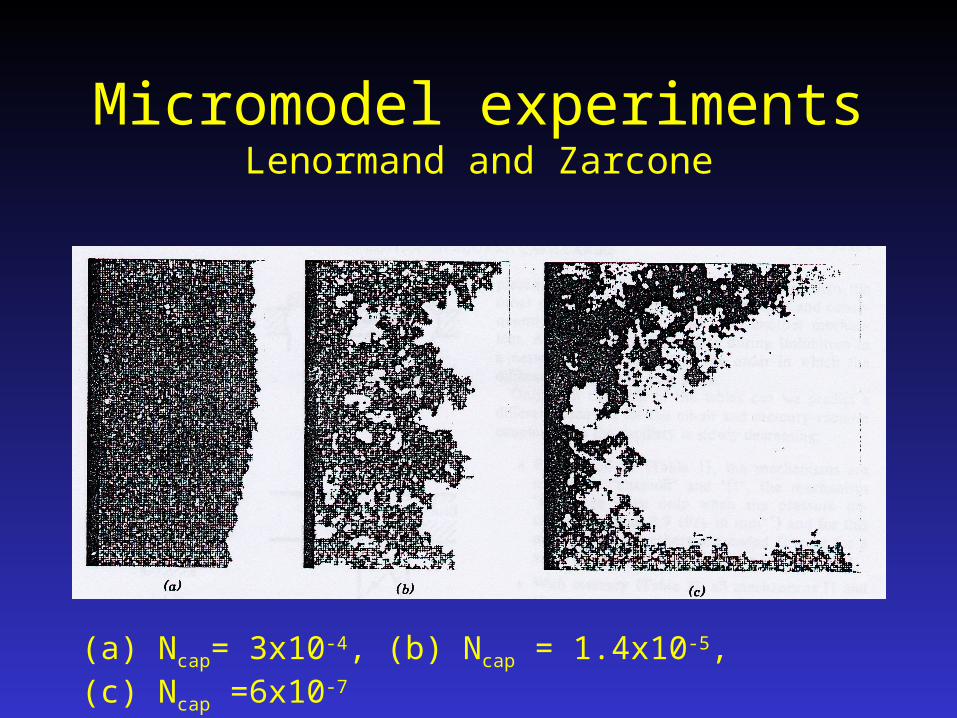
Micromodel experimentsLenormand and Zarcone
(a) Ncap= 3x10⁻⁴, (b) Ncap = 1.4x10⁻⁵, (c) Ncap =6x10⁻⁷
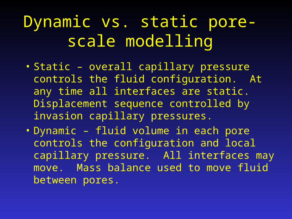
Dynamic vs. static pore-scale modelling
• Static – overall capillary pressure controls the fluid configuration. At any time all interfaces are static. Displacement sequence controlled by invasion capillary pressures.
• Dynamic – fluid volume in each pore controls the configuration and local capillary pressure. All interfaces may move. Mass balance used to move fluid between pores.
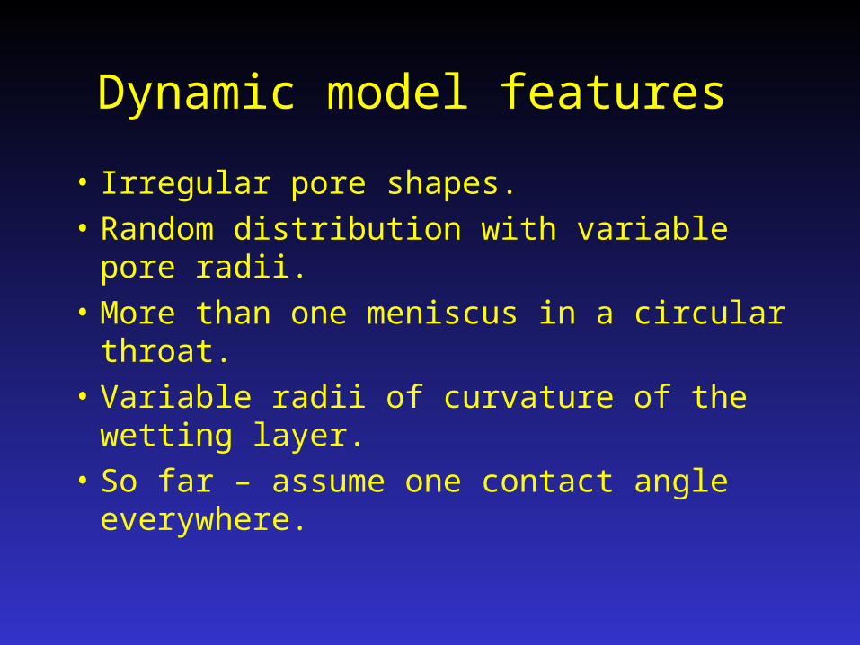
Dynamic model features
• Irregular pore shapes.
• Random distribution with variable pore radii.
• More than one meniscus in a circular throat.
• Variable radii of curvature of the wetting layer.
• So far – assume one contact angle everywhere.
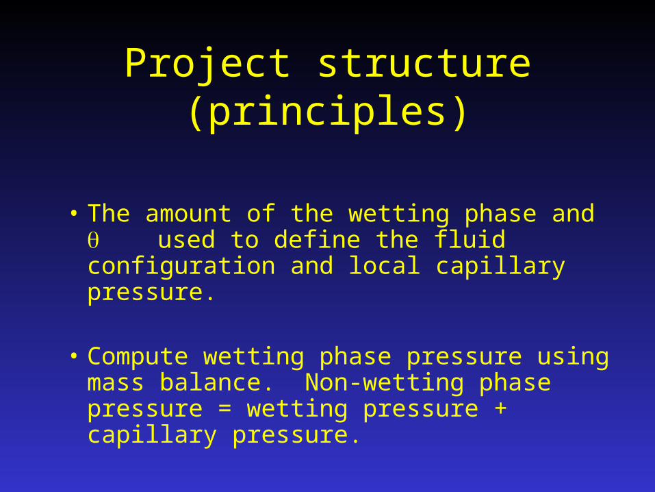
Project structure(principles)
• The amount of the wetting phase and used to define the fluid configuration and local capillary pressure.
• Compute wetting phase pressure using mass balance. Non-wetting phase pressure = wetting pressure + capillary pressure.
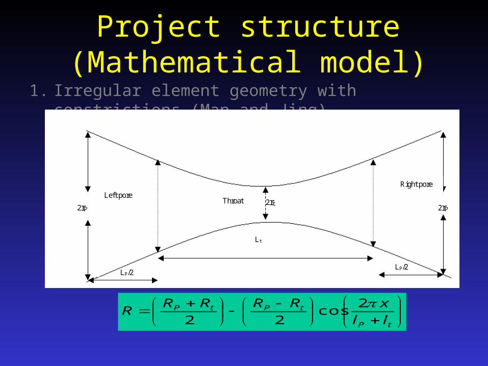
Project structure(Mathematical model)
1. Irregular element geometry with constrictions (Man and Jing).
2rP2rP
Left pore
Right pore
LP/2LP/2
Throat 2rt
Lt
tP
tPtP
ll
xRRRRR
2cos
22
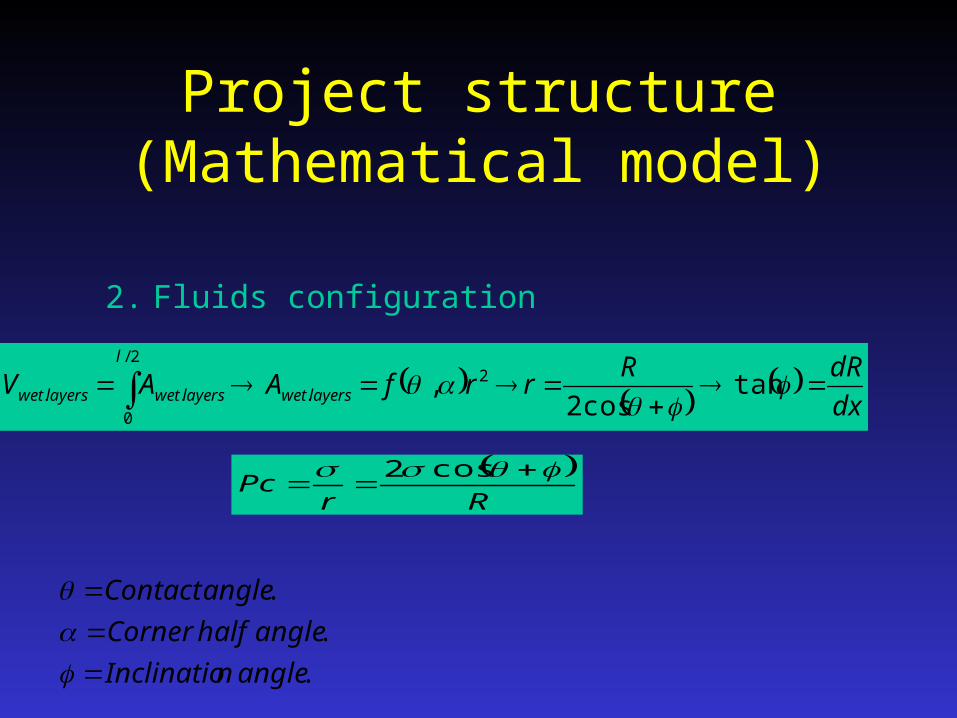
Project structure(Mathematical model)
2. Fluids configuration
dx
dRRrrfAAV layerswet
l
layerswetlayerswet
tancos2
, 2.
2/
0
..
Rr
Pc
cos2
.
.
.
anglenInclinatio
anglehalfCorner
angleContact
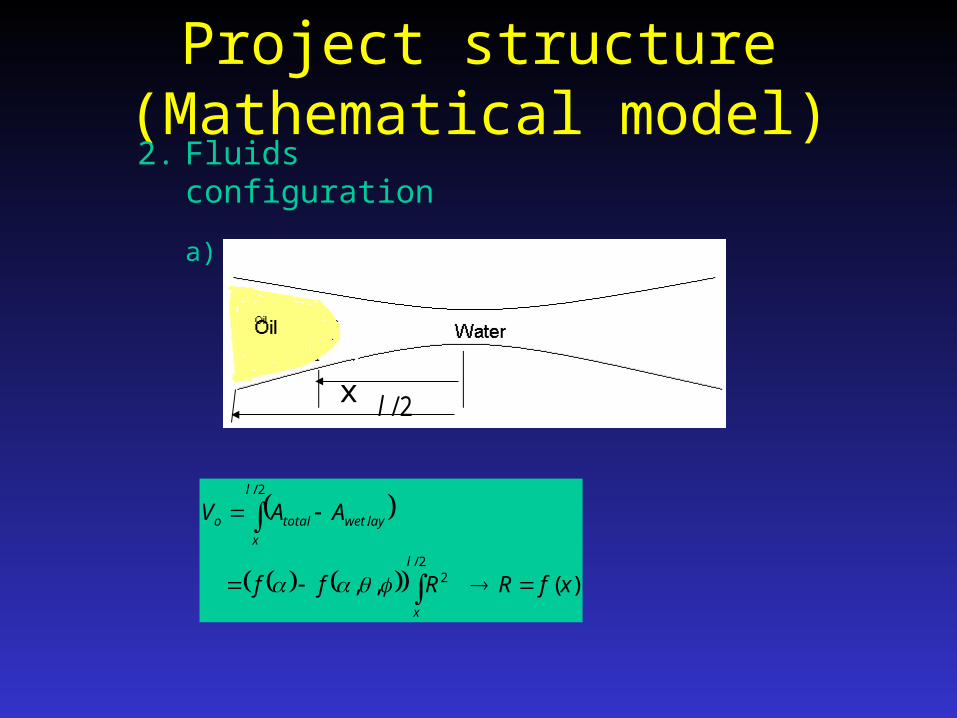
Project structure(Mathematical model)
2. Fluids configuration
a) General case:
x 2/l
)(,,2/
2
2/
.
xfRRff
AAV
l
x
l
x
laywettotalo
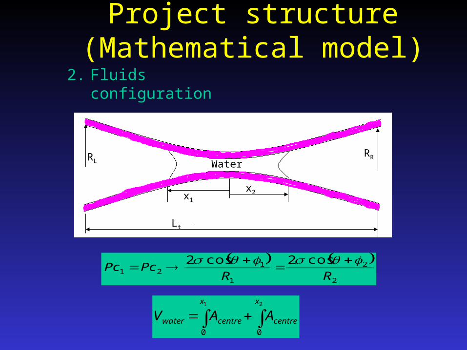
Project structure(Mathematical model)
2
2
1
121
cos2cos2
RRPcPc
1 2
0 0
x x
centrecentrewater AAV
2. Fluids configuration
b) special case:
Water
x2x1
Lt
RLRR
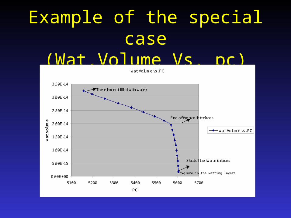
Example of the special case(Wat.Volume Vs. pc)
wat. Volume vs. PC
0.00E+00
5.00E-15
1.00E-14
1.50E-14
2.00E-14
2.50E-14
3.00E-14
3.50E-14
5100 5200 5300 5400 5500 5600 5700
PC
wa
t. v
olu
me
wat. Volume vs. PC
End of the two interfaces
Start of the two interfaces
The element filled with water
Volume in the wetting layers
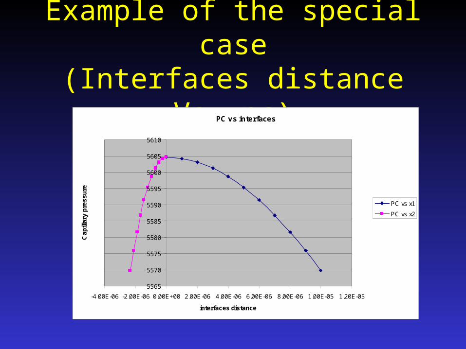
Example of the special case(Interfaces distance Vs. pc)
PC vs interfaces
5565
5570
5575
5580
5585
5590
5595
5600
5605
5610
-4.00E-06 -2.00E-06 0.00E+00 2.00E-06 4.00E-06 6.00E-06 8.00E-06 1.00E-05 1.20E-05
interfaces distance
Ca
pill
ary
pre
ss
ure
PC vs x1
PC vs x2
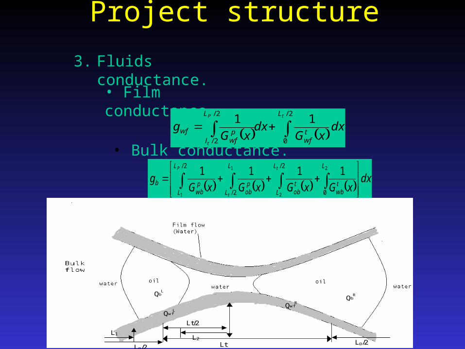
Project structure
3. Fluids conductance.
• Film conductance.
2/
0
2/
2/
11 tP
t
L
twf
L
lp
wfwf dx
xGdx
xGg
• Bulk conductance.
dxxGxGxGxG
gP
t
tL
L
L
L
L
L
L
twb
tob
pob
pwb
b
2/
2/
2/
01
1
2
2 1111
Lt
Lt/2
Q wf L Q wf R
Q b L Q b
R
Lp/2 Lp/2
L1 L2

Project structure(Mathematical model)
4. Computing the volumetric rates and pressures.
SPPg
QQQw
tw
P
oilwatertotal
o
c
g
PS
01
n
ii
wti
wPtotal SPPgQ
cappillarywateroil PPP
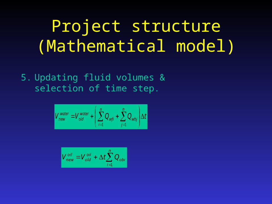
Project structure(Mathematical model)
5. Updating fluid volumes & selection of time step.
tQQVVn
i
n
jwbjwfi
waterold
waternew
1 1
n
iobi
oilold
oilnew QtVV
1
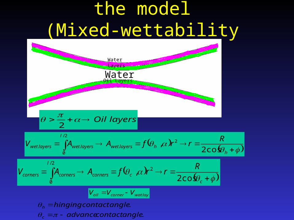
Future development of the model(Mixed-wettability system)
hhlayerswet
l
layerswetlayerswet
RrrfAAV
cos2, 2
.
2/
0
..
cccorners
l
cornerscorners
RrrfAAV
cos2, 2
2/
0
laywatcorneroil VVV .
.
.
anglecontactadvance
anglecontacthinging
c
h
Water Layers
Oil LayersWater
layersOil 2
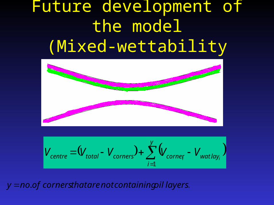
Future development of the model(Mixed-wettability system)
y
ilaywatcornercornerstotalcentre ii
VVVVV1
.
.. layersoilcontainingnotarethatcornersofnoy
Recap
• Presented methodology for a general rate-dependent pore-scale model.
• Shown how to compute configuration (interface location) and capillary pressure from known wetting phase volume.
• Next steps: compute conductance and from this use mass balance to move fluid between pores.