Embed Size (px)
Citation preview
POPULATION GROWTH AND ITS EFFECT ON LABOUR PRODUCTIVITY
IN GHANA
SUZZIE ABLORDEPPEY
Bachelor of Arts, Kwame Nkrumah University of Science and Technology, 2016
A thesis submitted
in partial fulfillment of the requirement for the degree
MASTER OF ARTS
in
ECONOMICS
Department of Economics
University of Lethbridge
LETHBRIDGE, ALBERTA, CANADA
© Suzzie Ablordeppey, 2021

POPULATION GROWTH AND ITS EFFECT ON LABOUR PRODUCTIVITY IN
GHANA.
SUZZIE ABLORDEPPEY
Date of Defence: June 7, 2021.
Dr. R. Mueller Professor Ph.D.
Thesis Supervisor
Dr. D. Rockerbie Professor Ph.D.
Thesis Examination Committee Member
Dr. K. Tran Professor Ph.D.
Thesis Examination Committee Member
Dr. D. Le Roy Associate Professor Ph.D.
Chair, Thesis Examination Committee

iii
ABSTRACT
This study analyzes population growth and its effect on labour productivity in
Ghana. In addition to the main objective, the study looks at the various factors
affecting overall labour productivity, labour productivity in the manufacturing and
agricultural sectors. The factors included in this study are government size, gross fixed
investment, human capital, inflation, and trade openness. The study is founded on the
data in Ghana from 1980-2019 by using the autoregressive distributed lag (ARDL)
model to define the long-run association between the variables. According to the
empirical evidence, increased population growth would reduce overall labour
productivity in Ghana’s economy in the long-run. No significant long-run impact was
observed between population growth rate and labour productivity in the
manufacturing sector. Finally, the research revealed that an increase in population
growth would have more than a proportionate fall on agricultural labour productivity
in the long-run.

iv
ACKNOWLEDGEMENTS
Firstly, I want to express my gratitude to the Almighty God for His grace
throughout my academic life and for making this thesis a success. My heartfelt thanks
go to my supervisor, Dr. R. Mueller, for his constructive comments, which helped to
improve this piece. To my father, Kwesi Ablordeppey, my brother, Kenny
Ablordeppey and my friend, Derrick Asafo-Adjei, thank you for your tremendous
support and encouragement. Finally, I would like to express my heartfelt appreciation
to Dr. D. Rockerbie and Dr. K. Tran, members of my thesis committee.

v
TABLE OF CONTENTS
Abstract .............................................................................................................................. iii
Acknowledgements ............................................................................................................. iv
Table of Contents ................................................................................................................. v
List of Tables ....................................................................................................................viii
List of Figures ..................................................................................................................... ix
CHAPTER 1 ........................................................................................................................ 1
1.1 Introduction ................................................................................................................ 1
1.2 Statement of Problem ................................................................................................. 4
1.3 Objectives of the Study .............................................................................................. 6
1.4 Research Questions .................................................................................................... 7
1.5 Significance of the Study ........................................................................................... 7
1.6 Organization of the Study .......................................................................................... 8
CHAPTER 2 ........................................................................................................................ 9
2.1 Theoretical Literature ................................................................................................. 9
2.1.1 Theories of Population ........................................................................................ 9
2.1.2 Human Capital Theory ...................................................................................... 12
2.2 Empirical Literature Review .................................................................................... 13
2.2.1 Empirical Evidence on Population and Economic Growth ............................... 13
2.2.2 Literature on Labour Productivity ..................................................................... 16

vi
2.2.3 Determinants of Labour Productivity ................................................................ 19
2.2.4 Literature on Labour Productivity in Ghana ..................................................... 25
CHAPTER 3 ...................................................................................................................... 27
3.1 Introduction .............................................................................................................. 27
3.2 Model Specification ................................................................................................. 27
3.3 Definition of Variables ............................................................................................. 28
3.3.1 Dependent Variables ......................................................................................... 30
3.3.2 Explanatory Variables ....................................................................................... 32
3.4 Data Sources ............................................................................................................ 35
3.5 Estimation Technique .............................................................................................. 35
3.5.1 Unit Root Tests .................................................................................................. 36
3.5.2 ARDL Bounds Test for Co-integration ............................................................. 37
3.6 Diagnostic Test ........................................................................................................ 42
3.7 Descriptive Statistics ................................................................................................ 46
CHAPTER 4 ...................................................................................................................... 49
4.1 Introduction .............................................................................................................. 49
4.2 Trend Analysis for Labour Productivity and other Key Variables .......................... 49
4.3 Unit Root Test .......................................................................................................... 52
4.4 ARDL Bounds Test for Cointegration ..................................................................... 54
4.5 Results of The Long-run and Short-run relationship ............................................... 57
4.5.1 Analysis of The Long and Short-run Estimates ................................................ 59
vii
4.6 Diagnostic Tests ....................................................................................................... 63
CHAPTER 5 ...................................................................................................................... 65
5.1 Introduction .............................................................................................................. 66
5.2 Summary of Research Findings ............................................................................... 66
5.3 Conclusion ............................................................................................................... 68
5.4 Limitations of the Study ........................................................................................... 68
5.5 Policy Recommendations ......................................................................................... 69
References .......................................................................................................................... 70
Appendix: Stability Test for Model 1-3 ............................................................................. 78

viii
LIST OF TABLES
Table 3.1: Description of Variables, their Acronyms, and Sources of Data………. 30
Table 3.2: Summary Statistics……………………………………………………… 46
Table 4.1: Stationarity Test Results…………………………………………………52
Table 4.2: Bounds Test Results…………………………………………………….. 55
Table 4.3: Long-run and Short-run Estimates……………………………………… 57
Table 4.4: Results of Diagnostic Tests………………………………………………63
ix
LIST OF FIGURES
Figure 2.1: Population and GDP Growth Rate from 1961-2019…………………… 15
Figure 4.1: Trend in Overall Labour productivity, Labour Productivity in the
Agricultural Sector, and Labour Productivity in the Manufacturing Sector in Ghana
(1980-2019)…………………………………………………………………………...49
Figure 4.2: Trend in The Growth of Labour Productivity, Human Capital, and
Population…………………………………………………………………………... ..51
Figure A.1: CUSUM and CUSUMSQ Test for Model 1……………………………..81
Figure A.2: CUSUM and CUSUMSQ Test for Model 2……………………………..82
Figure A.3: CUSUM and CUSUMSQ Test for Model 3……………………………..83
1
CHAPTER 1
1.1 Introduction
One fundamental factor influencing businesses' profit margin in most
developing countries and some advanced countries is labour productivity. The
variation in productivity rates in certain or all economic sectors affects the existence
and maintenance of inequality. Any attempt to reduce economic inequalities will mean
an investigation into the factors that help determine labour productivity. Polyzos and
Arabatzis (2006:4) saw productivity as an “expression of the degree of exploitation of
the most important coefficient in the productive process”. One of the most important
determining factors of an economy’s total output is productivity. Workforce
productivity is sought after in every economy to guarantee development. Quality
education is one important factor of labour productivity, which impacts development
in every economy. However, the degree of skills and knowledge positively affects
development compared to just educational accomplishment (Hanushek and
Woessman, 2020).
“Labour productivity is defined as the output level produced per unit of labour
inputs employed in production” (Kahyarara, 2020:1). Polyzos and Arabatzis (2006)
confirmed that the term is used interchangeably to depict labour productivity and other
production factors. Labour, technology, and capital are commonly calculated using the
ratio of outputs divided by the unit of input employed in the productivity activity. A
productive and efficient labour force is said to be the one that has developed the
necessary training and skills, and this leads to economic growth (Heshmati and
Rashidghalam, 2018). As the population of most developing countries increases, due
to high birth rates, it is expected that the amount of labour employed for economic
activities will also increase (Maestas, et al. 2016).
2
Some theories find a rise in population growth to adversely impact economic
growth with the explanation that, with immense population growth, each worker will
have other factors of production to work with (Hamza, 2015). Other theories suggest
that population growth will lead to greater labour productivity either by producing or
inducing innovations (Hamza, 2015). While some studies testing these theories have
found population growth to impact labour productivity positively, others found the
effect of population growth on labour productivity to be small or non-existent.
Population growth in most sub-Saharan African countries is alarming as most of them
are not equipped to handle the dramatically increased needs for food, water, sanitation,
education, and employment. Slower growth in population will guarantee that more
individuals will gain access to social amenities and medical care (Population Impact
Project, 1994).
The population dynamics of most developing countries keep changing due to
the rising birth rate as against the low death rate which hinders development.
Economic activities within most African countries have increased and due to that, the
demand for labour has also increased. As indicated by Kahyarara (2020), most
developing countries rely on the agricultural sector and activities in this sector are
concentrated in the rural areas. In Ghana, most of the people who migrate to the urban
centres are in the informal sector and economic activities within the informal and
agricultural sectors are predominantly reliant on unskilled labour. 60% of employment
is contributed by the informal sector with about 90% from the micro-and medium-
scale sectors, despite the recent increase in economic growth in South Africa, Ghana,
Uganda, and Tanzania (Danquah, Schotte and Sen, 2019). An increase in the amount
of labour is, however, expected to either affect labour productivity negatively or
positively (Hamza, 2015).
3
Amade and Bakari (2019) also indicates that although the theoretical
association between output (GDP) and population growth is negative, empirically the
relationship is inconclusive. However, recent studies show that due to technological
advancement and population growth countries such as India and China have
experienced development. This benefit has allowed for more workforce participation
and, ultimately, increasing productivity (Kahyarara, 2020). India, and China are
countries that have contradicted this position as population seems to affect growth
positively.
There are numerous studies on the impact of population growth on economic
growth in most sub-Saharan African countries (e.g., Akintunde, Olomola and Oladeji,
2013; Cist, Mora and Engelman, 2017; Hamza, 2015) but the exact relationship
between population growth on economic growth in these countries remain to be
inconclusive. The difference in these studies lies in how economic growth is measured
and the methodology and estimation technique used.
In calculating economic growth, much research has used GDP or GDP per
capita (Amade and Bakari, 2019; Rahman, et al. 2017; Azuh, et al. 2016). While the
connection between economic growth and population has been largely examined,
studies examining the link between population growth and labour productivity have
been fewer. According to Kahyarara (2020), the few studies that sought to investigate
the impact of population growth on labour productivity have brought about some
controversies in their labour productivity measurement. The first controversy is how
best to measure output, and the second is defining labour input. The two options are
the value-added and the gross output. The gross output is “the number of goods and
services produced while ignoring the total intermediate inputs used” (Attar, et al.

4
2012). This research looks at Ghana’s population growth on labour productivity by
measuring labour productivity as gross output per employed person (GDPPEP).
Similar to this is the empirical study of Guest and Swift (2008).
1.2 Statement of Problem
Studies show that countries such as India, China, and Brazil have proved that
countries have profited from increased labour force growth from an increased
population. The influence of population growth rate on macro and microeconomic
factors has been well established in the literature. The investigation focuses on
economic growth, labour force participation, manufacturing productivity, and
agricultural productivity. Since the publication of Rev. Malthus' work on population in
1798, the impacts of population growth on economic parameters have been subjected
to empirical debate. Some people argue that population has a positive correlation with
labour productivity, some argue that the relationship is negative, and others believe
that the relationship between the two is insignificant. Dawson (1998:149) pointed out
that most textbooks on development economics have sections dedicated to the
connection between population and growth. They highlight the importance of the
population to the development of an economy. According to Thornton (2001) and
Amade and Bakari (2015), population growth can affect diverse ways of economic
performance. Population growth is one of the ways through which productivity is
affected.
Productivity is one of the ways through which the output of the economy can
be increased. This is because increased productivity enhances overall growth hence
helping to reduce poverty and unemployment, improving living standards and well-
being. Labour is central in development process and the process of learning new skills
5
and gaining information that is relevant to a specific technology. All productivity
measures share the relationship between output and inputs required in production
(Boadu, 1994). The question asked is how much output is produced by each unit of
labour, which gives rise to the definition of labour productivity. Such a definition of
labour productivity has brought much argument concerning how best to measure
productivity and define labour input.
According to Attar, et al. (2012), there is no universally accepted definition
and measurement for labour productivity. The definition and measurement of
productivity can center on the individual, the firm, and the whole economy. Kahyarara
(2020) states that to measure labour productivity, gross domestic product (GDP) and
value-added measures have been the widely used measures of productivity. The GDP
measure of productivity focuses on the number of goods and services produced
without considering the intermediate inputs used. According to Attar, et al. (2012), the
reliance on gross output as a measure of labour productivity is mainly due to the
availability of data. Studies that use gross output do not struggle to get data to be used
as a proxy for labour productivity. Much of the concentration has been on value-added
and gross output (e.g., Kahyarara 2020; Hamza 2015).
While most literature has focused widely on economic growth and population
growth in most Asia and Latin American Countries (LAC) (e.g., Thornton, 2001;
Hsieh, 2002; Timmer and Akkus, 2008; Adullah, et al. 2015; Üngor, 2017) quite a
number have also concentrated on Africa and sub-Saharan Africa (e.g., Amade and
Bakari, 2015; Hamza, 2015; Rahman, et al. 2017). However, the connection between
population and labour productivity has not been examined in Ghana.
Concerning population growth and labour productivity, much emphasis has
then again been placed on Latin American countries (LAC) and Asia countries (e.g.,
6
Jha, 2006; Imai, Gaiha and Bresciani, 2018; Dua and Garg, 2017) and on some
African countries (e.g., Polyzos and Arabatzis, 2006; Diao, et al. 2018; Kahyarara,
2020). Studies' examining the connection between population growth and labour
productivity have not been few in Ghana. There is, therefore, the need to investigate
the impact that population growth rate has on labour productivity in Ghana. With the
Statistical Service of Ghana estimating the country's total population to be about 30
million, it is important to examine if the growth in population is equivalent to a higher
level of labour productivity within the agricultural and manufacturing sectors of
Ghana since the agriculture sector employs about 60% of the population and the
manufacturing sector 23% (GSS, 2015). In addition to the above, this study further
examines the disagreement among several other studies on population growth and its
effect on labour productivity in Ghana.
1.3 Objectives of the Study
The main goal of the research is to examine how population growth affect
labour productivity. Specifically, this research seeks to:
1. Identify the factors influencing labour productivity in Ghana.
2. Examine the trend analysis on labour productivity and some
determinants of labour productivity.
3. Examine the factors that affect the agricultural sector’s labour
productivity in the long run.
4. Examine the factors that determine the manufacturing sector’s labour
productivity in the long run.
7
1.4 Research Questions
1. What are the determinants of labour productivity?
2. What is the trend between labour productivity and some of the
determinants of labour productivity?
3. What are the factors that affect labour productivity in the agricultural
and manufacturing sectors in the long run?
1.5 Significance of the Study
The study of population growth and its effect on labour productivity in Ghana
has much significance. Several factors determine labour productivity, and quite a
number of studies have examined various determinants of labour productivity,
especially in Latin America (LAC), Asia, North America and Middle East. These
studies have either been examined at the individual, the firm, and the economy level.
Surprisingly, there has been no study conducted within the Ghanaian context. This
thesis will add to the literature by examining the extent to which population growth
affects labour productivity in the Ghanaian economy and help identify the factors
responsible for determining labour productivity in Ghana. Also, we will investigate
factors responsible for labour productivity in the agricultural and manufacturing
sectors and how that impacts the economy. With this evidence the policymakers will
be able to make sector-specific, agricultural, and manufacturing policies that will go a
long way to affect overall productivity and economic growth. Again, this study is
significant because it will contribute in several says to this area of study.

8
1.6 Organization of the Study
This thesis is divided into five chapters, with the first chapter capturing the
introduction, background, problem statement, objectives, research questions, the
significance and the organization of the study. The relevant theoretical and empirical
literature is reviewed in chapter two. The methods, data, and procedures are discussed
in chapter 3. Presentation and discussion of results are done with reference to the
literature in chapter four. The summary, conclusions and policy recommendations are
presented in chapter five.
9
CHAPTER 2
2.1 Theoretical Literature
This section looks at theories put forward to explain population growth and
labour productivity.
2.1.1 Theories of Population
Pessimistic Theory
The pessimistic theory can be traced back to an essay written by English
scholar Reverend Thomas Malthus in 1798, titled “An Essay on the Principle of
Population”. In the face of an ever-increasing population, Malthus wondered whether
society could change in the future. He came to the popular conclusion that the
demands of a rapidly increasing population would soon overwhelm food production.
To put it another way, “the scenario of arithmetic increases in food production
combined with simultaneous exponential or geometric increases in population
expected a future in which humans will be unable to feed themselves”. According to
Malthus, population growth could reduce per capita output because the output growth
rate cannot match up with the population growth rate (Landreth and Colander, 1989).
Thus, although population growth is supposed to increase output per capita there will
be more people added to the workforce and this will lead to the limitation or
unavailability of capital and decreasing marginal returns to labour (Landreth and
Colander, 1989). To maintain the natural balance between production and
consumption, he asserted that preventive and positive controls on population growth
are needed (Malthus, 1826).

10
An extension to Malthus' theory was a work by Ehrlich (1968) in his book
titled "The Population Bomb" where he predicted that millions of people will die of
starvation in the 1970s due to overpopulation. He asserted population control as the
only way to save humanity from self-destruction. Many pessimists believe that
reducing population is the most significant step toward increasing economic growth,
and improving living conditions (Easterlin, 1997). A significant amount of research
has projected that population growth would have a net negative impact. The
pessimistic theory implies that a rise in population growth would have a detrimental
impact on labour productivity.
Pessimistic advocates explain that, in relation to the effects of overall
population growth on wealth, there is possible negative relationship between capital
and population growth in an economy (Palumbo, et al. 2010). Increased population
necessitates the renting of more factories and the construction of more facilities to
meet the needs of people in the economy, which could result in lower standard of
living.
Optimistic Theory
Optimistic theory can be found in the work of Danish economist Ester
Boserup, who used similar claims to transform the Malthusian view. Rather than being
influenced by agriculture, as Malthus (1798) believed, Boserup (1996) claimed that
growth in population is a positive determinant of agricultural productivity. The study
argued against the assumption of Malthus and claimed that higher population growth
might lead to an efficient division of labour and increase agricultural productivity.
“Necessity is the mother of invention”, she stated, because population growth puts
11
strain on resources, it will encourage people to be resourceful and innovative,
particularly in difficult times (Boserup, 1996).
According to Kuznets (1960:2), “an increase in population will lead to an
increase in the labour force of an economy”. He claimed that “if the labour force
grows at the same level as population, it would be able to produce the same amount of
output or more output per labour”.
Another criticism of Malthus’ theory, which predicted misfortune as
population grows, is Julian Simon’s book, “The Ultimate Resource”. Simon (1976)
claimed that technological progress was dependent on population size, and that a
rising population continues to advance in knowledge overtime, increasing
productivity. He came to the conclusion that as population grows, people will continue
to create new resources, recycle old ones, and find new creative solutions. As a result,
the idea that population growth would lead to human stagnation was wrong.
The Neutralist Theory
The neutralist theory’s underlying principle is that population growth is
independent of output (Bloom, et al. 2003). Since the mid-1980s, the neutralist theory
has become the dominant viewpoint (Bloom and Freeman, 1988). Despite the
variations within the neutralist school, the National Academy of Sciences (NAS)
maintained that “slower population growth would be beneficial to the economic
development of most developing countries” (National Research Council, 1986).
According to Kelley (2001), natural resources negatively affect population growth
since, as population grows, natural resources are depleted as people require more
farmlands, space for habitation, and a variety of other activities. The optimistic theory
of population growth did not look into this. Multi-country research found no proof of

12
pessimists’ perceived resource diversification from more efficient sector to less
productive sectors such as education, medical care and safety measures. According to
Kelley (2001), the results of these findings, along with the claims by Simon and
Bartlett (1985), were significant reasons for the progress of neutralist ideas. The
authors claim that, “the scarcity of resources increases the cost of a product, thereby
creating the incentive to find alternative materials”.
2.1.2 Human Capital Theory
Human capital is characterized as "productive wealth embodied in labour,
skills and knowledge" (OECD, 2001), and it refers to acquired knowledge, or
characteristics related to an individual (Garibaldi, 2006). The idea that education
which is referred to as human capital has an economic effect started from a consistent
research program in the 1950s. Allan Fisher (1946) emphasized the importance of
considering education on economic policy. Human capital, according to Becker
(1997), is described as "activities that influence future monetary and income by
increasing resources in people" with schooling and on-the-training as the most
common types.
Human capital theory, as established by Schultz (1971), Sakamota and Powers
(1995) and Psacharopoulos and Woodhall (1997), is based on the premise that
education is extremely useful and even indispensable for improving an individual’s
production ability. In a nutshell, human capital researchers argue that a well-educated
population is more profitable since thispopulation is perceived to boost production in
an economy. Human capital theory emphasizes how education boosts people's
efficiency and competitiveness by enhancing efficient human capability, which is a
result of investment and natural abilities. The acquisition of formal schooling and
13
training demonstrates an efficient investment in human resources, which the theory’s
authors consider to be more equally valuable than physical capital, since physical
capital only has to do with the investments in assets, such as buildings, machinery and
vehicles used in production processes. These also need experienced and well-educated
labour to operate, which is the outcome of human capital.
The theory proposes that as investment in human capital rises then the
individual is expected to engage in the labour market (Becker, 1997). This is due to
the fact that skills and expertise increase an individual’s productivity and therefore
their earning power in the labour market. As a result, people with higher education
would be more active and make more money on the job than people with lower
education.
2.2 Empirical Literature Review
2.2.1 Empirical Evidence on Population and Economic Growth
This section reviews literature on the relationship between population growth
and economic growth. It is critical to examine the relationship between population and
economic growth since population is believed to be an incentive for production and
could have a positive impact on output and productivity.
Dao (2012) used data from World Bank’s World Development Indicators on
43 countries to examine the economic effect of demographic change in developed
countries and discovered that population growth is positively linked to GDP per
capita. Several other studies have found the negative impact of population growth on
GDP growth rate. Hamza (2015) used GDP growth rate to determine how economic
growth and population growth are linked and indicated a significant negative
relationship between economic growth and population growth. Hamza used panel data
14
on a cross-section of 30 developing countries for 14-years, with these countries
selected from Africa, Asia, and Latin America. Population parameters such as birth
rates, death rates and net migration were negatively related to economic growth, with
only the death rate being statistically significant. Similar results were observed by
Cist, Mora and Engelman (2017) and Akintunde, Olomola and Oladeji (2013) who
also observed that most sub-Saharan African countries have a negative relationship
between economic growth and population growth.
Brückner and Schwandt (2015) performed a panel data analysis covering 139
countries from 1960-2007, looking at the income-population relationship. The two
variables had a positive relationship, according to the researchers. The relationship
indicates that when population in a country rises, GDP per capita growth rises as well.
Nwosu, et al. (2014) and Tartiyus, et al. (2015), found a long run significant positive
effect between economic growth and population growth.
Abdullah, et al. (2015) found the opposite results in Bangladesh. Their
findings, based on data from 1980 to 2005 and a multiple linear regression model,
show that economic growth and population growth are negatively related, meaning
that an increase in Bangladesh’s population would have a negative effect on the
country’s economic growth.
The figure below shows the link between population and GDP growth rate in
Ghana.

15
Figure 2.1: Population and GDP growth rate from 1961-2019
Source: World Bank, WDI (2020)
Figure 2.1 shows the population and GDP growth rate for Ghana. The key
drivers of Ghana’s population growth are fertility rate, death rate and net migration. In
Ghana, migration from other countries to Ghana is extremely rare, with only few cases
of migration from countries within Africa. Ghana's population growth rate has been
stable from 1984 after a drastic decline in growth rate in 1975, the lowest the country
has ever witnessed. The drastic decline in GDP growth rate in 1975 was due to
political unrest and upheavals. The post-independence conditions of the country were
better, with the highest growth rate in 1962 (3.21%), declining to 2.29% in 1968. This
rose further to 2.81% in 1972, declining drastically to 1.85% in 1978. Thereafter, the
population growth rate has been stable. According to Jong-a-Pin (2009), a high level
of political uncertainty delays economic growth. Darko (2015) confirms that the time
between the 1970s and the early 1980s was highly volatile due to political turmoil,
which had a great impact on the GDP growth rate. Darko (2015: 4) reports Anyemedu
(1993) as indicating that "the economy of Ghana was nearly at the verge of collapse in
1983 when the inflation rate was high to 123%". Darko (2015:4) indicates that,
although Anyemedu indicates that "this was as a result of the devastating drought
-15
-10
-5
0
5
10
15
20
19
61
19
64
19
67
19
70
19
73
19
76
19
79
19
82
19
85
19
88
19
91
19
94
19
97
20
00
20
03
20
06
20
09
20
12
20
15
20
18
Pro
po
rtio
n (
An
nu
al %
)
GDP growth (annual %) Population growth (annual %)
16
which reduced the production of main agricultural commodities and other export crops
like cocoa", clearly, from the population growth rate observed above, the period of
slow economic growth corresponded to rising population growth rates. When the
population growth rate was declining from 1975, with the lowest growth rate in 1977,
the economy was growing at a rate of 8.48 %. At the lowest growth rate of -12.48%,
population growth rate was fairly stable. This shows that population had no significant
impact on economic growth. The highest growth rate experienced by the country was
14.07% in 2011 when the country commenced oil production. From thence, economic
growth has been declining sharply, with a lower economic growth rate of 2.27% in
2015 rising thereafter.
2.2.2 Literature on Labour Productivity
Using data from the Groningen Growth and Development Centre, Diao, et al.
(2018) looked at the level of agricultural and industrial sectors productivity of a few
African countries. For countries that have effectively industrialized, the authors
discovered a positive association between the manufacturing and agricultural labour
productivities. Similarly, Schultz (1953) stated that advancement in agricultural
productivity is necessary for improving sustained economic growth for countries with
a closed economy. This became the benchmark for several other studies
predominantly featured (Johnson and Kilby, 1975; Johnson and Mellor,1961). Unlike
Schultz (1953), Lewis (1954) believes that low agriculture labour productivity will
continue until non-agricultural labour force expands to absorb population growth in
the rural sector, and that industrialization will easily help increase productivity in the
agriculture sector by reducing the amount of labour in the sector. Several other studies
have analyzed the relationship between agricultural productivity and economic growth
17
concentrating on an open economy rather than the closed economy model (e.g.,
Matsuyama, 1992; Wright, 1979).
Settsu and Takashima (2020) examined labour productivity growth and its
long run impact in Japan from 1600 to 1909 using regional panel data for sector share.
The results suggest that the Tokugawa period’s industrial system was fairly stable.
They show that an increase in population provides adequate labour for different
sectors of the economy, resulting in increased performance.
Broadberry and Irwin (2005) also looked at whether labour efficiency in the
US and UK differed during the 19th century. According to the authors, the UK had
higher efficiency of labour in the industrial sector while the US had higher efficiency
of labour in the service sectors. The agricultural labour efficiency on the other hand,
was comparable in both countries. The conclusion from the findings was that the UK
had higher aggregate labour efficiency in the industrial sector, and the US had a higher
share of the work force in the low value-added agricultural sector in the mid-
nineteenth century.
Moussir and Chatri (2019) examined the differences in labour productivity
between the traditional and modern sectors of the Moroccan economy by investigating
the structural changes of the economy using an input-output model. The authors found
that structural change, which is the reallocation of resources from the agricultural
sector to the non-agricultural sector of the country, has significantly impacted the
overall level of labour productivity growth which is explained largely by intra-sector
growth. They indicate that although overall labour productivity growth for the country
has improved, there are some aspects of the economy that makes use of unskilled
labour in the traditional sectors. Timmer and Akkus (2008) showed that structural
18
transformation, especially among developing countries through investment in human
capital, improved technologies, and lowered transaction costs, facilitated the
integration of economic activities and the efficient allocation of resources, and hence
improved labour productivity. Also, the United Nations Industrial Development
Organization (UNIDO, 2012) says that structural transformation of an economy is a
key source of productivity growth and increased per capita income.
Jha (2006) also examined agricultural labour productivity in India with
changes in the real wages of agricultural workers while investigating the movement
out of agricultural employment. The findings show that the proportion of women
working in agriculture is decreasing, resulting in a drop in labour productivity.
Concerning the movement out of agricultural employment, both small, marginal
farmers, and agricultural workers have been moving between and within work and
regions. This, therefore, could not result in a balance in the regional development of
agriculture. Although the study examined female labour productivity in the
agricultural sector, it did not investigate the factors influencing labour productivity.
Imai, Gahia and Bresciani (2018) investigated the gap between labour
productivity within the agricultural and non-agricultural sectors of thirty-seven Asian
countries using panel data. The findings suggest that for some selected Asian
countries, the gap within the agricultural and non-agricultural sectors has widened.
The authors, however, did not investigate the determinants of labour productivity
among the thirty-seven Asian countries, including India.
Using the World Bank’s Enterprise Survey database for 2013, Heshmati and
Rashidghalam (2018) investigated the effect of labour productivity on the service and
manufacturing sectors of Kenya’s economy. The authors found that as the ratio of

19
female-to-male workers in the labour force increases, labour productivity declines.
While the study identified the factors that influence labour productivity, they did not
examine the difference in labour productivity for the manufacturing sector.
2.2.3 Determinants of Labour Productivity
This section assesses the empirical evidence on the determinants of labour
productivity.
One of the key determining factor of the profitability, competitiveness and the
growth of enterprises, firms, and/or businesses is labour productivity. Some
international organizations mention the importance of labour productivity. The United
Nations noted the importance of labour productivity through one of its Sustainable
Development Goals (SDGs) target. Labour productivity is the most essential
component of production (OECD, 2001). It is also mentioned by the International
Labour Organization (ILO) that labour productivity measures efficiency to produce
goods and services and reflects the standards of living (ILO, 2016). Therefore, it is
necessary to analyze the determinants of labour productivity.
A study by Dua and Garg (2017) identified the determinants of labour
productivity in developed and developing countries. The authors used panel
cointegration and group-mean fully modified ordinary least squares estimation to
analyze the data. The result showed that trade openness, technology, capital,
government spending and human capital significantly affect labour productivity in
developed and developing countries, but the impact is different.
Population growth impacts the environment, economy, and society in different
ways; for developed, and developing countries, according to Rawat (2014). Kahyarara
20
(2020), using time series data from 1967 to 2012 and a Cobb-Douglas production
function, examined the effects of population growth on economy-wide productivity.
The author analyzed how changes in population increased labour force participation
which led to an increase in productivity. Findings from the study revealed a positive
effect of population on labour productivity after controlling for other inputs like raw
materials and capital. Because of the positive effects of population growth on the
economy through increased productivity, the author advocates for the need to intensify
labour productivity in the establishment of new economic enterprises and or
businesses. Rawat (2014) found that population impacts productivity positively and
hence on the economic growth rate, however, this varies at country level since
countries vary in their endowments. The relationship is negative for China, India,
Japan, Nigeria, and Brazil, but positive for United States, Pakistan, Bangladesh,
Russia and Mexico.
Goedhuys, et al. (2014) looked into the factors that influence productivity in
Tazanian manufacturing firms. Using cross-sectional data at the firm level, the authors
examined how advancement in technology and the environment in which firms
operate affect their efficiency. They found that among the technological variables,
research and development (R&D), innovation, technology, and training of employees
have no impact on productivity, but rather higher educational level of management
and foreign ownership have an impact.
Fallahi, et al. (2010) used a cross-sectional regression model with a sample of
12,299 manufacturing firms to investigate the determinants of labour productivity.
The authors found that labour productivity and education, R&D activity, wage, capital
per employee, and export orientation of the labour force are positively related. They
21
noted further that, although R&D expenditure of the firm, the level of information
technology (IT) of the firm, and the size of the firm are widely recognized factors that
affect the productivity of labour, it is education, and training of human resources that
"has a special place over the above-mentioned factors" (Fallahi, et al. 2010: 3). They
believe that a well-educated labour force is capable of operating physical capital as
well as creating or using new technology in the production process. And, as such, any
activity of the firm that is not geared towards expanding the skill and knowledge base
of labour would imply a reduction in the profitability of the firm due to the increased
cost of production. Similarly, Aggrey, et al. (2014) stated that human capital
development contributes significantly to output and labour productivity just like any
other factors of production such as technology and innovation. They were quick to add
that the latter is dependent on the development of human capital through education
and training. Also, Mahmood and Afza (2008) indicated that secondary education
enrollment had a positive effect on total factor productivity.
Corvers (1997), in discussing the determinants of labour productivity,
identified education and training as one of the unique determinants of labour
productivity. He identified four effects that human capital has on labour productivity.
These four effects include worker effect, allocation effect, diffusion effect, and
research effect. To him, these four effects work to determine the quality of labour for
an enterprise or business. He indicated that it is through the allocation effect and
worker effect that human resources contribute to the level of productivity and the
growth of productivity through diffusion and research effects.
Another determinant of labour productivity widely investigated in literature is
the capital of the firm. Wijaya (2019) found that capital formation, a proxy to capital,
22
has a positive impact in the short run and long-run on the productivity of labour.
According to the study, higher capital formation led to higher labour productivity, i.e.,
higher capital formation itself can be generated from an improvement in a total of the
net inventory changes and fixed asset accumulation such as construction of railways,
roads, public and private buildings, machinery, and land improvements. Similarly,
Papadogonas and Voulgaris (2005), in examining the effect of capital equipment on
industrial firms of Greece, found that increasing the capital equipment of firms causes
labour productivity to improve.
Using dynamic ordinary least squares to analyze panel data from 1980-2014,
Samargandi (2018) examined the determinants of labour productivity in North Africa
and Middle East countries. The author found that human capital and capital stock
positively impacts labour productivity. Furthermore, it was found by the author that
financial growth, trade openness and industrial value addition have a substantial effect
in boosting labour productivity, and innovation is an important factor in increasing
labour productivity.
According to Jiang (2010), trade openness has a positive impact on labour
productivity in China. The author used a dynamic panel data approach and compiled
data from 29 provinces in China over the period 1984 to 2008. Also, Saha (2012)
studied the effect of trade openness on total factor productivity in India. Applying
ordinary least squares and Granger causality tests, the results showed that there was a
one-way relationship and a significantly positive effect between trade openness and
total factor productivity. On the contrary, Ishmail, et al. (2011) found trade openness
have a negative and substantial impact on labour productivity. The authors employed
panel data and a multiple regression model to estimate labour productivity in the
23
Malaysian manufacturing industries from 1985 to 2008. The result indicated that
globalization indicators such as trade openness and foreign direct investment had a
significant negative effect on labour productivity. Although Irwin and Tervio (2002),
Rodriguez and Rodrik (2001), and Rodrik (2000) argued that trade openness is an
insignificant determinant of labour productivity, particularly when a proxy to capital is
used or when quality of institutions and climate controls are included in the empirical
study.
Many economists believe that high inflation rates create distortions that result
in unproductive resource allocation and hence reduce productivity (Sbordone and
Kuttner, 1994). In consequence, as they examined the post war relationship between
inflation and productivity in the US, they found a negative relationship between
inflation and labour productivity resulting from a monetary contraction where
inflation remains high as output contracts. They explained that each one percent
increase in the annual inflation rate was accompanied by a reduction in labour
productivity growth of about one-quarter percent per year. Following this are
theoretical reasons that inflation has been the major cause of productivity slowdown,
such that Konya, et al. (2019) for 22 OECD countries established that productivity
increase also induces inflation to fall. On the contrary, Freeman and Yerger’s (2000)
analysis with 12 countries of the OECD did not support the assertion that there exists
an inverse relationship between inflation and labour productivity growth. In their
bivariate and multivariate tests of inflation and productivity, they revealed no proof of
a consistent relationship between inflation and productivity growth.
Smoluk and Andrews (2005) in examining the factors that affect labour
productivity among 48 states in the US from 1993 to 2000, used a Constant Elasticity

24
of Substitution (CES) production function framework by building upon the empirical
study of Carlino and Voith (1992). The authors concentrated on the impact of
population density and education on labour productivity while introducing a state tax
burden variable in the empirical model. Their findings show that labour productivity is
positively related to the percentage of population with a bachelor's degree.
Wijaya (2019), using time series data from 1978 to 2017 and an ARDL model,
identified government expenditure as a determinant of labour productivity in
Indonesia. In the study, he observed that in both the short run and long run,
government expenditure had a positive effect on labour productivity. The findings
indicate that a rise in government spending will lead to an enhancement in labour
productivity, but the findings are contradictory to Dua and Garg (2017), who provided
evidence of a negative impact of government expenditure on labour productivity in
both upper-middle-income economies and developed economies. In the case of lower-
middle economies, their analysis gave the same results. Awotunde (2018) proved that
government expenditure that goes into labour issues such as health affects labour
productivity positively. Hence, spending more on sectors that are related to labour
issues such as health, education and training programs, social etc., seems to be the
channel through which labour productivity can be encouraged.
Dhiman and Sharma (2017) also looked into the Indian textile industry’s
productivity patterns and determinants. The study used labour and capital productivity
levels in the Indian textile industry to examine how efficient labour and capital were,
as well as their effect on the economy. The study found that both labour and capital
productivity levels in industries have been decreasing, using a time series regression
model with a cointegration test. According to the authors, productivity varies by
25
industry and is dependent to a large extent on the productive existence of labour and
capital in the Indian labour market.
2.2.4 Literature on Labour Productivity in Ghana
Teal (1999) discovered that there had been no increase in technical efficiency
among Ghanaian companies, but that production growth had been balanced by
sufficient increases in labour and capital inputs. He also discovered no evidence that
smaller businesses expand at a faster rate than larger businesses. Also, Sodërbom and
Teal (2004) accessed the impact of the level of technology and allocative efficiency in
the manufacturing sector. They found that large firms face a far higher relative cost of
labour than small firms; hence labour productivity is higher for large manufacturing
firms in Ghana. Using a Crépon-Duguet-Mairesse (CDM) structural model to examine
the effect of innovation on 501 manufacturing firms in Ghana, Xiaolan, et al. (2018)
found a positive effect of innovations on manufacturing firms in Ghana. They indicate
that informal firms are less productive compared to formal firms, and that innovations
affect the productivity level of formal firms more than informal firms. Similarly,
Agyapong, et al. (2017) found a positive association between different forms of
innovation and success in small and medium enterprises in Ghana in a cross-sectional
analysis of 500 micro and small-scale businesses.
Codjoe (2006) investigated the effects of population dynamics in Ghana’s
Volta basin, and found that there had been a rapid rise in population in these areas
between 1960 and 2010. The size of the agricultural labour force, as well as
productivity, increased as the Volta basin’s population grew rapidly. The rise in
population also increased the availability and engagement of labour in agriculture,
26
forest reserves and water resources along the Volta basin, and this trend is expected to
continue as the majority of people in the area are drawn to this sector.
Aragón and Rud (2011) examined the extent to which pollution from
manufacturing industries affects agricultural productivity. Using an agricultural
production function, the authors showed that agricultural lands for farming purposes
located in areas close to industries had their total factor productivity reduced by
almost 40 percent between 1997-2005. This means that industrial pollution has a
negative effect on agricultural labour productivity. In addition, Hanna and Olivia
(2011) and Graff and Neidell (2012) found that air pollution negatively affects labour
supply and agricultural productivity.
The findings from the empirical literature on how population growth predicts
labour productivity is inconclusive. In Ghana, the majority of the studies that have
examined population growth have limited the study to economic growth, which is
measured by either Gross Domestic Product (GDP), and or GDP per capita. However,
there are no studies that address the relationship between population growth and
labour productivity in the case of Ghana. To date, only one study has looked into this
problem with the Tanzanian population. Since the labour force structures in Tanzania
and Ghana are so close, it is reasonable to believe that the relationship between
population and labour productivity found in Tanzania can also be found in Ghana.
Therefore, having a deeper understanding of the condition of population and labour
productivity in Ghana is necessary to fill the gap and contribute to further policy
decisions.
The next chapter goes through the data sources, variables, and research
methods that will be used for the estimations.
27
CHAPTER 3
3.1 Introduction
This chapter discusses the methodology and data employed for the study. More
specifically, it describes the empirical model underpinning the effects of population
growth and some determinants of Ghana's labour productivity. The study further
examines labour productivity in the agriculture and manufacturing sectors. It discusses
some of the determinants of labour productivity in these two sectors as these two
sectors are labour-intensive. It also discusses the econometric techniques used in
addressing the research questions, specifies the models to be estimated, and describes
the variables employed for the study, the sources of data, and the means of estimating
the various parameters.
3.2 Model Specification
In this study, the empirical model used is similar to Wijaya (2019) and Dua
and Garg (2017). The study specifies labour productivity as a function of population
growth, government size, trade openness, inflation, human capital, and gross fixed
investment. The study defines labour productivity to be gross domestic product per the
number of people employed, consistent with the work of Wijaya (2019). The
equations below show that labour productivity is influenced by inflation, government
size, trade openness, human capital, gross fixed investment, and population growth.
The study further estimates two separate models using labour productivity in
the agricultural and manufacturing sectors to determine some of the determinants of
labour productivity in the sectors where all variables are as defined in equation 3.1.
The separate models in 3.2 and 3.3 will help capture the different effects of all the
variables defined on Ghana's labour productivity in two sectors of the economy.
28
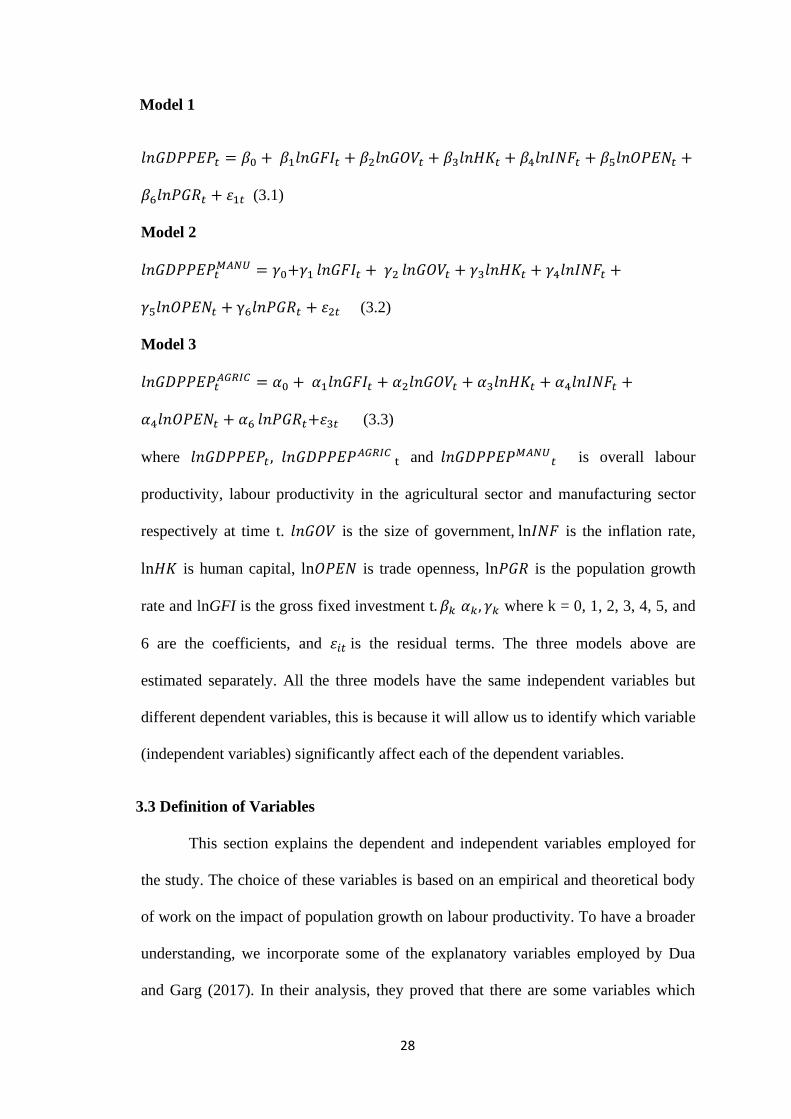
Model 1
𝑙𝑛𝐺𝐷𝑃𝑃𝐸𝑃𝑡 = 𝛽0 + 𝛽1𝑙𝑛𝐺𝐹𝐼𝑡 + 𝛽2𝑙𝑛𝐺𝑂𝑉𝑡 + 𝛽3𝑙𝑛𝐻𝐾𝑡 + 𝛽4𝑙𝑛𝐼𝑁𝐹𝑡 + 𝛽5𝑙𝑛𝑂𝑃𝐸𝑁𝑡 +
𝛽6𝑙𝑛𝑃𝐺𝑅𝑡 + 휀1𝑡 (3.1)
Model 2
𝑙𝑛𝐺𝐷𝑃𝑃𝐸𝑃𝑡𝑀𝐴𝑁𝑈 = 𝛾0+𝛾1 𝑙𝑛𝐺𝐹𝐼𝑡 + 𝛾2 𝑙𝑛𝐺𝑂𝑉𝑡 + 𝛾3𝑙𝑛𝐻𝐾𝑡 + 𝛾4𝑙𝑛𝐼𝑁𝐹𝑡 +
𝛾5𝑙𝑛𝑂𝑃𝐸𝑁𝑡 + γ6𝑙𝑛𝑃𝐺𝑅𝑡 + 휀2𝑡 (3.2)
Model 3
𝑙𝑛𝐺𝐷𝑃𝑃𝐸𝑃𝑡𝐴𝐺𝑅𝐼𝐶 = 𝛼0 + 𝛼1𝑙𝑛𝐺𝐹𝐼𝑡 + 𝛼2𝑙𝑛𝐺𝑂𝑉𝑡 + 𝛼3𝑙𝑛𝐻𝐾𝑡 + 𝛼4𝑙𝑛𝐼𝑁𝐹𝑡 +
𝛼4𝑙𝑛𝑂𝑃𝐸𝑁𝑡 + 𝛼6 𝑙𝑛𝑃𝐺𝑅𝑡+휀3𝑡 (3.3)
where 𝑙𝑛𝐺𝐷𝑃𝑃𝐸𝑃𝑡 , 𝑙𝑛𝐺𝐷𝑃𝑃𝐸𝑃𝐴𝐺𝑅𝐼𝐶 t and 𝑙𝑛𝐺𝐷𝑃𝑃𝐸𝑃𝑀𝐴𝑁𝑈
𝑡 is overall labour
productivity, labour productivity in the agricultural sector and manufacturing sector
respectively at time t. 𝑙𝑛𝐺𝑂𝑉 is the size of government, ln𝐼𝑁𝐹 is the inflation rate,
ln𝐻𝐾 is human capital, ln𝑂𝑃𝐸𝑁 is trade openness, ln𝑃𝐺𝑅 is the population growth
rate and lnGFI is the gross fixed investment t. 𝛽𝑘 𝛼𝑘, 𝛾𝑘 where k = 0, 1, 2, 3, 4, 5, and
6 are the coefficients, and 휀𝑖𝑡 is the residual terms. The three models above are
estimated separately. All the three models have the same independent variables but
different dependent variables, this is because it will allow us to identify which variable
(independent variables) significantly affect each of the dependent variables.
3.3 Definition of Variables
This section explains the dependent and independent variables employed for
the study. The choice of these variables is based on an empirical and theoretical body
of work on the impact of population growth on labour productivity. To have a broader
understanding, we incorporate some of the explanatory variables employed by Dua
and Garg (2017). In their analysis, they proved that there are some variables which

29
had a significant impact on labour productivity such as gross fixed investment (proxy
for capital), human capital, government expenditure, institutional quality, and trade
openness. Regarding the data availability, we use human capital, population growth,
gross fixed investment, size of government, inflation, and trade openness. The
description of these variables and their sources of data are provided in Table 3.1

30
Table 3. 1 Description of Variables, their acronyms, and sources of data (1980- 2019).
VARIABLES ACRONYM DESCRIPTION EXPECTED
SIGNS
SOURCE(S) OF
DATA
Labour
productivity GDPPEP
The ratio of real
GDP (measured
in constant 2010
prices) to the
total number of
employed
persons (between
15-64 years)
World Bank
Development
Indicators (WDI,
2019), Ghana
Statistical Service
(GSS,2019)
Labour
productivity in
the
agricultural
sector
GDPPEPAGRIC
The GDP
contribution of
the agricultural
sector per unit of
an employed
person (between
15-64 years) in
the sector
WDI (2019), GSS
(2019)
Labour
productivity in
the
manufacturing
sector
GDPPEPMANU
The GDP
contribution of
the
manufacturing
sector per unit of
an employed
person (between
15-64 years) in
the sector
WDI (2019), GSS
(2019)
Population
growth rate PGR
Annual
percentage
change in a
country's
population
- WDI (2019)
Inflation INF
Annual
percentage
change in
consumer price
index (CPI)
- WDI (2019)
Trade
openness OPEN
Trade openness
is the sum of
exports and
imports of goods
and services
measured as a
percentage of
GDP
+ WDI (2019)
Human capital HK
Human capital is
measured as
gross enrolment
in secondary and
tertiary
education
+ WDI (2019)
Government
size GOV
The general
government final
consumption
- WDI (2019)

31
expenditure is
expressed as a
ratio of GDP
Gross fixed
investment GIF
The annual
percentage
change in capital
stock (it includes
land
improvements,
plants and
machinery)
+ WDI (2019)

32
3.3.1 Dependent Variables
The dependent variables in this study are labour productivity, and labour
productivity in the agriculture and manufacturing sectors.
Following Guest and Swift (2008), labour productivity is a continuous variable
that is measured as gross domestic product (GDP) per employed person (between 15-
64 years).
Manufacturing and agricultural labour productivity is measured by computing
the total output of the agricultural and manufacturing sectors divided by the number of
people employed (between 15-64 years) within the sector.
3.3.2 Explanatory Variables
3.3.2.1 Population Growth Rate (PGR)
Several studies have found a connection between labour productivity and
population growth. 'Population optimists' believe that increased population makes
labour more innovative and makes countries take advantage of economies of scale,
both of which increase labour productivity. It is also believed that population growth
reduces the number of resources available to labour and hence makes labour
unproductive. However, it is unclear whether there is a negative or positive
relationship with labour productivity. The average percentage change in population is
used to calculate the population growth rate.
3.3.2.2 Size of Government (GOV)
The size of government is considered as a fiscal indicator that is important in
determining productivity within an economy. The effect of this indicator on
productivity can either be beneficial or harmful depending on the level of efficiency of
33
government expenditure. For instance, when the government sector competes with the
private sector for existing limited resources, productivity might be reduced if the
government does not spend efficiently (Dua and Garg, 2017). However, if government
expenditure is efficient, this might translate into an increase in private sector
investment and result in higher productivity levels, other factors being held constant.
A study by Awotunde (2018) proved that government expenditure that goes to health
affects labour productivity positively. Hence, spending more on sectors which are
related to labour issues such as health, education and training program, social, etc.
seems to be a channel through which labour productivity can be encouraged. Landau
(1983), on the other hand, found that the share of government expenditure on
consumption affects labour productivity hence economic growth negatively.
Therefore, the impact of the government size is calculated in terms of
government consumption expenditure as a percentage of GDP (Loko and Diouf,
2009).
3.3.2.3 Inflation (INF)
Inflation is defined as “the persistent increase in the general price level of
goods and services over a period”. Various authors such as Banerji and Dua (2004),
and Tang (2014) have assessed the effect of inflation on labour productivity. Anytime
there is increased inflation, it is assumed that resources are diverted to unproductive
activities that are the cost of fighting inflation rather than towards activities that
improve productivity (Jarrett and Selody, 1982). A persistent increase in the price
level results in uncertainties that discourage the urge to invest by the private sector. In
situations where investments are carried out, inputs are not combined to achieve their
34
maximum outputs, which impacts the productivity of labour and other inputs in the
long run.
3.3.2.4 Human Capital (HK)
Human capital is measured by the gross enrollment in secondary and tertiary
education in the country (Dua and Garg, 2017). This includes vocational and technical
education. Several studies on productivity have established the positive relationship
between human capital and productivity.
3.3.2.5 Trade Openness (OPEN)
The summation of exports and imports as a percentage of GDP is the measure
of trade openness. It is argued that an economy that opens up to the rest of the world
tends to benefit from the resources of other parts of the world. For instance, a country
that opens up and imports machinery and other capital goods can build the economy's
technological base, which in turn increases productivity. Additionally, an economy
that exports its goods and services to other parts of the world enjoys the benefit of
producing more goods and services when demand increases. Also, localized
businesses become competitive, which in turn improves their productivity.
Comparative advantage theory argues that international trade makes an
economy produce more output in areas where it has a comparative advantage. Studies
on the effect of trade openness on labour productivity show that trade openness has a
significant positive effect on labour productivity (e.g., Valadkhani, 2005; Dimelis and
Papaioannou, 2010; and Fraga, 2016), while some others obtained the opposite result.
Follmi, et al. (2018) discovered that real and nominal trade openness is not
significantly related to labour productivity in Switzerland at the aggregate level, and
35
Ishmail, Rosa and Sulaiman (2011) using manufacturing industries found a negative
relationship between trade openness and labour productivity in Malaysia.
3.3.2.6 Gross Fixed Investment (GFI)
Capital is a key variable in production, and it refers to assets or goods that
have already been produced and are used in the production of other goods and
services. Gross fixed investment as a percentage of GDP is used as proxy for capital
in this study, and it represents percentage change in capital stock over a period. This is
believed to affect labour productivity as labour tends to be more productive with an
increase in the share of capital used in the production process.
3.4 Data Sources
The data for this study is sourced from the World Bank World Development
Indicators (WDI) database and the Ghana Statistical Service (GSS) database. All the
variables are sourced from World Bank World Development Indicators except
employment which is sourced from the GSS. The employment data is sourced from
GSS due to the availability of data for the time period which is not available in the
WDI database. The dependent variables are labour productivity, and labour
productivity in the manufacturing and agricultural sectors. The explanatory variables
are population growth, government size, human capital, inflation, trade openness and
gross fixed investment. Annual data spanning from 1980-2019 are employed in the
study. The selection of the time period is largely based on data availability.
3.5 Estimation Technique
The variables are subjected to preliminary tests to ensure that the parameters
calculated using time series data from the described econometric model are consistent
36
and accurate. The tests consist of stationarity and cointegration tests. The former will
help us avoid estimating a spurious regression, while the latter will help establish
cointegration among the variables in the models (i.e., whether there is a long run
impact among the variables).
3.5.1 Unit Root Tests
Stationarity tests are important when studying time series data because
macroeconomic data usually tend to either increase or decrease over time and might
also be trended, thus making it possible for time-series data to be non-stationary. The
stationarity test helps us test for model specification to avoid misleading conclusions
from a spurious regression analysis. The study employed the two most robust and
commonly used stationarity tests for time series data (i.e., the Phillips-Perron (PP) and
the Augmented Dickey-Fuller (ADF) tests) since they ensure that the test for
stationarity is more reliable than other tests of stationarity. The ADF and PP tests are
identical, but they vary in how they deal with autocorrelation in the error term. The PP
test is used to solve the problem of heteroscedasticity but the ADF test does not solve
this problem. The PP test, unlike the ADF test, assumes that the error terms are
weakly dependent and heterogeneously distributed, yielding more accurate estimates
than the ADF which assumes the error terms are independent. In addition, with the PP
test, we do not need to define the lag length for the test regression.
Unit root test are used to avoid spurious estimation, which is a common
problem when working with time series data (Gujarati, 2007). It is also needed for
analyzing long-run connections between two or more time-series data (Engle and
Granger, 1987). For example, the autoregressive distributed lag (ARDL) bounds test
needs that the variables be incorporated of order one, order zero or a combination of
37
both, and this is confirmed by the unit root test. The stationarity properties of each of
the variables in question are tested with and without a time trend and constant. The
Akaike Information Criterion and the Newey- West bandwidth selects the automatic
lag length for the ADF and PP tests.
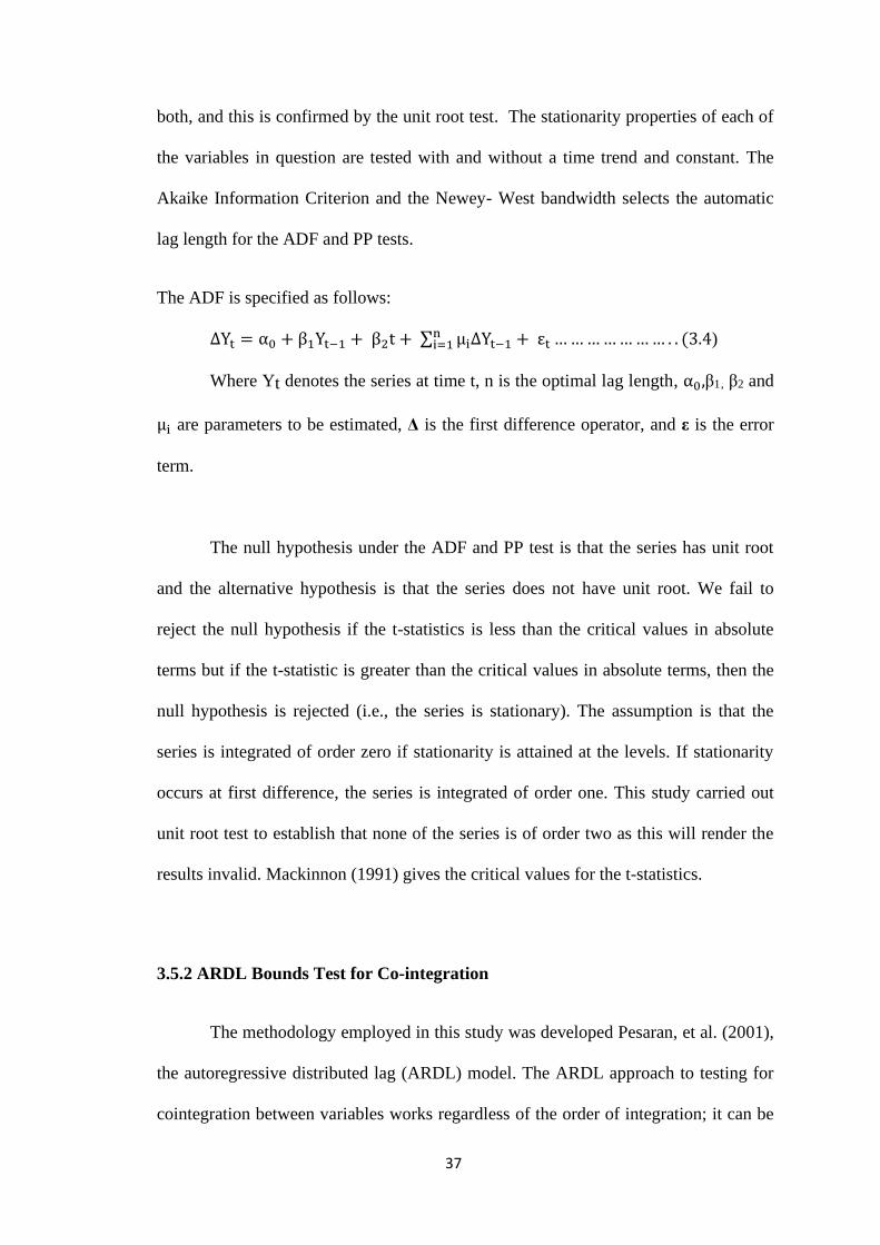
The ADF is specified as follows:
∆Yt = α0 + β1Yt−1 + β2t + ∑ µi∆Yt−1ni=1 + εt … … … … … … … . . (3.4)
Where Yt denotes the series at time t, n is the optimal lag length, α0,β1, β2 and
µi are parameters to be estimated, Δ is the first difference operator, and ε is the error
term.
The null hypothesis under the ADF and PP test is that the series has unit root
and the alternative hypothesis is that the series does not have unit root. We fail to
reject the null hypothesis if the t-statistics is less than the critical values in absolute
terms but if the t-statistic is greater than the critical values in absolute terms, then the
null hypothesis is rejected (i.e., the series is stationary). The assumption is that the
series is integrated of order zero if stationarity is attained at the levels. If stationarity
occurs at first difference, the series is integrated of order one. This study carried out
unit root test to establish that none of the series is of order two as this will render the
results invalid. Mackinnon (1991) gives the critical values for the t-statistics.
3.5.2 ARDL Bounds Test for Co-integration
The methodology employed in this study was developed Pesaran, et al. (2001),
the autoregressive distributed lag (ARDL) model. The ARDL approach to testing for
cointegration between variables works regardless of the order of integration; it can be
38
integrated of order one I (1), I (0) or a combination of both. The ARDL bounds test
approach to cointegration is chosen over other approaches like Engle and Granger
(1987) and Johansen (1991) because of its multiple advantages.
The ARDL bounds test is a useful method for determining cointegration
relationship in a small sample. The ARDL bounds test can also be used to establish an
unrestricted error correction model through a simple linear change. The error
correction model combines the short run dynamics and the long run equilibrium
without sacrificing long run information.
The results from the bounds test will determine if we are to specify either
short-run (ARDL model) or both short-run and long-run (error correction model)
model. Hence, if the results show that the variables are cointegrated then we specify
both the short-run and long-run models. We only use the short-run (ARDL) model if
the variables are not cointegrated.
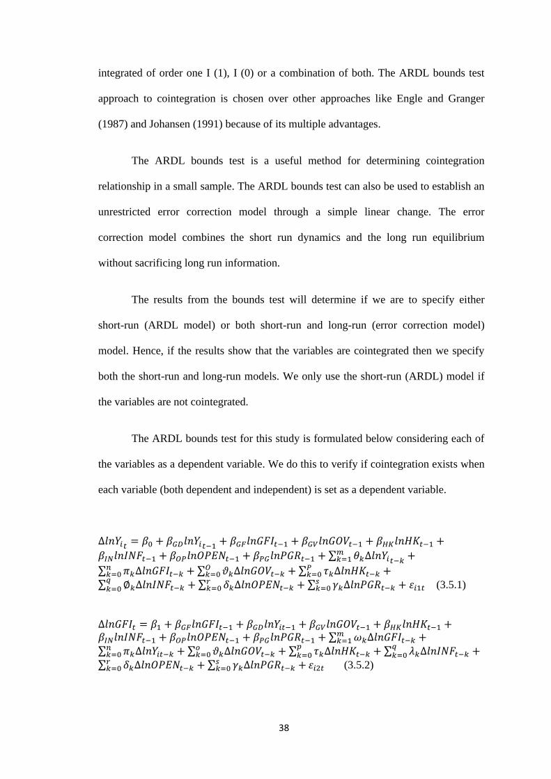
The ARDL bounds test for this study is formulated below considering each of
the variables as a dependent variable. We do this to verify if cointegration exists when
each variable (both dependent and independent) is set as a dependent variable.
∆𝑙𝑛𝑌𝑖𝑡= 𝛽0 + 𝛽𝐺𝐷𝑙𝑛𝑌𝑖𝑡−1
+ 𝛽𝐺𝐹𝑙𝑛𝐺𝐹𝐼𝑡−1 + 𝛽𝐺𝑉𝑙𝑛𝐺𝑂𝑉𝑡−1 + 𝛽𝐻𝐾𝑙𝑛𝐻𝐾𝑡−1 +
𝛽𝐼𝑁𝑙𝑛𝐼𝑁𝐹𝑡−1 + 𝛽𝑂𝑃𝑙𝑛𝑂𝑃𝐸𝑁𝑡−1 + 𝛽𝑃𝐺𝑙𝑛𝑃𝐺𝑅𝑡−1 + ∑ 𝜃𝑘∆𝑙𝑛𝑌𝑖𝑡−𝑘𝑚𝑘=1 +
∑ 𝜋𝑘∆𝑙𝑛𝐺𝐹𝐼𝑡−𝑘𝑛𝑘=0 + ∑ 𝜗𝑘∆𝑙𝑛𝐺𝑂𝑉𝑡−𝑘
𝑂𝑘=0 + ∑ 𝜏𝑘∆𝑙𝑛𝐻𝐾𝑡−𝑘
𝑃𝑘=0 +
∑ ∅𝑘∆𝑙𝑛𝐼𝑁𝐹𝑡−𝑘𝑞𝑘=0 + ∑ 𝛿𝑘∆𝑙𝑛𝑂𝑃𝐸𝑁𝑡−𝑘
𝑟𝑘=0 + ∑ 𝛾𝑘∆𝑙𝑛𝑃𝐺𝑅𝑡−𝑘
𝑠𝑘=0 + 휀𝑖1𝑡 (3.5.1)
∆𝑙𝑛𝐺𝐹𝐼𝑡 = 𝛽1 + 𝛽𝐺𝐹𝑙𝑛𝐺𝐹𝐼𝑡−1 + 𝛽𝐺𝐷𝑙𝑛𝑌𝑖𝑡−1 + 𝛽𝐺𝑉𝑙𝑛𝐺𝑂𝑉𝑡−1 + 𝛽𝐻𝐾𝑙𝑛𝐻𝐾𝑡−1 +𝛽𝐼𝑁𝑙𝑛𝐼𝑁𝐹𝑡−1 + 𝛽𝑂𝑃𝑙𝑛𝑂𝑃𝐸𝑁𝑡−1 + 𝛽𝑃𝐺𝑙𝑛𝑃𝐺𝑅𝑡−1 + ∑ 𝜔𝑘Δ𝑙𝑛𝐺𝐹𝐼𝑡−𝑘
𝑚𝑘=1 +
∑ 𝜋𝑘Δ𝑙𝑛𝑌𝑖𝑡−𝑘𝑛𝑘=0 + ∑ 𝜗𝑘Δ𝑙𝑛𝐺𝑂𝑉𝑡−𝑘
𝑜𝑘=0 + ∑ 𝜏𝑘Δ𝑙𝑛𝐻𝐾𝑡−𝑘
𝑝𝑘=0 + ∑ 𝜆𝑘Δ𝑙𝑛𝐼𝑁𝐹𝑡−𝑘 +𝑞
𝑘=0
∑ 𝛿𝑘Δ𝑙𝑛𝑂𝑃𝐸𝑁𝑡−𝑘 + ∑ 𝛾𝑘Δ𝑙𝑛𝑃𝐺𝑅𝑡−𝑘 +𝑠𝑘=0
𝑟𝑘=0 휀𝑖2𝑡 (3.5.2)
39
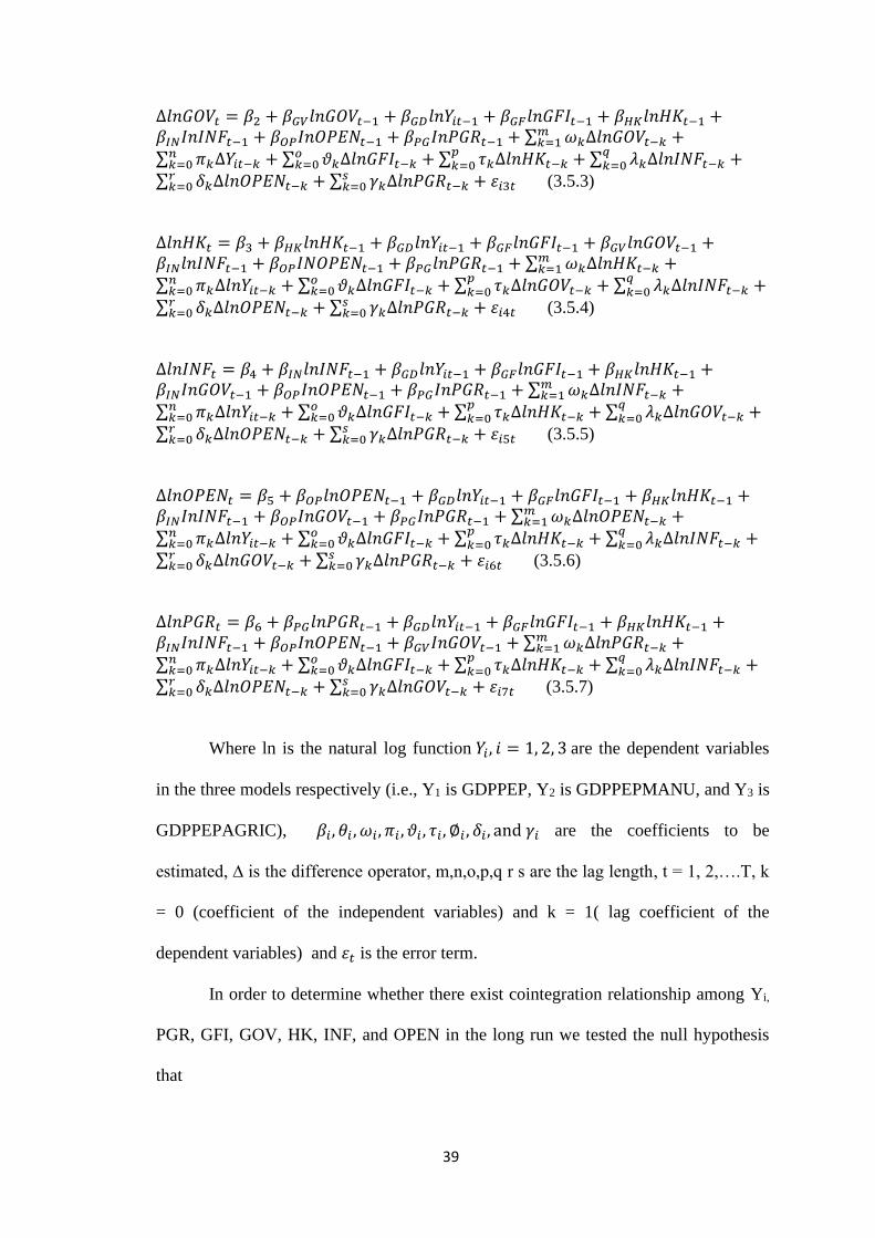
∆𝑙𝑛𝐺𝑂𝑉𝑡 = 𝛽2 + 𝛽𝐺𝑉𝑙𝑛𝐺𝑂𝑉𝑡−1 + 𝛽𝐺𝐷𝑙𝑛𝑌𝑖𝑡−1 + 𝛽𝐺𝐹𝑙𝑛𝐺𝐹𝐼𝑡−1 + 𝛽𝐻𝐾𝑙𝑛𝐻𝐾𝑡−1 +𝛽𝐼𝑁𝐼𝑛𝐼𝑁𝐹𝑡−1 + 𝛽𝑂𝑃𝐼𝑛𝑂𝑃𝐸𝑁𝑡−1 + 𝛽𝑃𝐺𝐼𝑛𝑃𝐺𝑅𝑡−1 + ∑ 𝜔𝑘Δ𝑙𝑛𝐺𝑂𝑉𝑡−𝑘
𝑚𝑘=1 +
∑ 𝜋𝑘Δ𝑌𝑖𝑡−𝑘𝑛𝑘=0 + ∑ 𝜗𝑘Δ𝑙𝑛𝐺𝐹𝐼𝑡−𝑘
𝑜𝑘=0 + ∑ 𝜏𝑘Δ𝑙𝑛𝐻𝐾𝑡−𝑘
𝑝𝑘=0 + ∑ 𝜆𝑘Δ𝑙𝑛𝐼𝑁𝐹𝑡−𝑘
𝑞𝑘=0 +
∑ 𝛿𝑘Δ𝑙𝑛𝑂𝑃𝐸𝑁𝑡−𝑘𝑟𝑘=0 + ∑ 𝛾𝑘Δ𝑙𝑛𝑃𝐺𝑅𝑡−𝑘
𝑠𝑘=0 + 휀𝑖3𝑡 (3.5.3)
∆𝑙𝑛𝐻𝐾𝑡 = 𝛽3 + 𝛽𝐻𝐾𝑙𝑛𝐻𝐾𝑡−1 + 𝛽𝐺𝐷𝑙𝑛𝑌𝑖𝑡−1 + 𝛽𝐺𝐹𝑙𝑛𝐺𝐹𝐼𝑡−1 + 𝛽𝐺𝑉𝑙𝑛𝐺𝑂𝑉𝑡−1 +𝛽𝐼𝑁𝑙𝑛𝐼𝑁𝐹𝑡−1 + 𝛽𝑂𝑃𝐼𝑁𝑂𝑃𝐸𝑁𝑡−1 + 𝛽𝑃𝐺𝑙𝑛𝑃𝐺𝑅𝑡−1 + ∑ 𝜔𝑘Δ𝑙𝑛𝐻𝐾𝑡−𝑘
𝑚𝑘=1 +
∑ 𝜋𝑘Δ𝑙𝑛𝑌𝑖𝑡−𝑘𝑛𝑘=0 + ∑ 𝜗𝑘Δ𝑙𝑛𝐺𝐹𝐼𝑡−𝑘
𝑜𝑘=0 + ∑ 𝜏𝑘Δ𝑙𝑛𝐺𝑂𝑉𝑡−𝑘
𝑝𝑘=0 + ∑ 𝜆𝑘Δ𝑙𝑛𝐼𝑁𝐹𝑡−𝑘
𝑞𝑘=0 +
∑ 𝛿𝑘Δ𝑙𝑛𝑂𝑃𝐸𝑁𝑡−𝑘𝑟𝑘=0 + ∑ 𝛾𝑘Δ𝑙𝑛𝑃𝐺𝑅𝑡−𝑘
𝑠𝑘=0 + 휀𝑖4𝑡 (3.5.4)
∆𝑙𝑛𝐼𝑁𝐹𝑡 = 𝛽4 + 𝛽𝐼𝑁𝑙𝑛𝐼𝑁𝐹𝑡−1 + 𝛽𝐺𝐷𝑙𝑛𝑌𝑖𝑡−1 + 𝛽𝐺𝐹𝑙𝑛𝐺𝐹𝐼𝑡−1 + 𝛽𝐻𝐾𝑙𝑛𝐻𝐾𝑡−1 +𝛽𝐼𝑁𝐼𝑛𝐺𝑂𝑉𝑡−1 + 𝛽𝑂𝑃𝐼𝑛𝑂𝑃𝐸𝑁𝑡−1 + 𝛽𝑃𝐺𝐼𝑛𝑃𝐺𝑅𝑡−1 + ∑ 𝜔𝑘Δ𝑙𝑛𝐼𝑁𝐹𝑡−𝑘
𝑚𝑘=1 +
∑ 𝜋𝑘Δ𝑙𝑛𝑌𝑖𝑡−𝑘𝑛𝑘=0 + ∑ 𝜗𝑘Δ𝑙𝑛𝐺𝐹𝐼𝑡−𝑘
𝑜𝑘=0 + ∑ 𝜏𝑘Δ𝑙𝑛𝐻𝐾𝑡−𝑘
𝑝𝑘=0 + ∑ 𝜆𝑘Δ𝑙𝑛𝐺𝑂𝑉𝑡−𝑘
𝑞𝑘=0 +
∑ 𝛿𝑘Δ𝑙𝑛𝑂𝑃𝐸𝑁𝑡−𝑘𝑟𝑘=0 + ∑ 𝛾𝑘Δ𝑙𝑛𝑃𝐺𝑅𝑡−𝑘
𝑠𝑘=0 + 휀𝑖5𝑡 (3.5.5)
∆𝑙𝑛𝑂𝑃𝐸𝑁𝑡 = 𝛽5 + 𝛽𝑂𝑃𝑙𝑛𝑂𝑃𝐸𝑁𝑡−1 + 𝛽𝐺𝐷𝑙𝑛𝑌𝑖𝑡−1 + 𝛽𝐺𝐹𝑙𝑛𝐺𝐹𝐼𝑡−1 + 𝛽𝐻𝐾𝑙𝑛𝐻𝐾𝑡−1 +𝛽𝐼𝑁𝐼𝑛𝐼𝑁𝐹𝑡−1 + 𝛽𝑂𝑃𝐼𝑛𝐺𝑂𝑉𝑡−1 + 𝛽𝑃𝐺𝐼𝑛𝑃𝐺𝑅𝑡−1 + ∑ 𝜔𝑘Δ𝑙𝑛𝑂𝑃𝐸𝑁𝑡−𝑘
𝑚𝑘=1 +
∑ 𝜋𝑘Δ𝑙𝑛𝑌𝑖𝑡−𝑘𝑛𝑘=0 + ∑ 𝜗𝑘Δ𝑙𝑛𝐺𝐹𝐼𝑡−𝑘
𝑜𝑘=0 + ∑ 𝜏𝑘Δ𝑙𝑛𝐻𝐾𝑡−𝑘
𝑝𝑘=0 + ∑ 𝜆𝑘Δ𝑙𝑛𝐼𝑁𝐹𝑡−𝑘
𝑞𝑘=0 +
∑ 𝛿𝑘Δ𝑙𝑛𝐺𝑂𝑉𝑡−𝑘𝑟𝑘=0 + ∑ 𝛾𝑘Δ𝑙𝑛𝑃𝐺𝑅𝑡−𝑘
𝑠𝑘=0 + 휀𝑖6𝑡 (3.5.6)
∆𝑙𝑛𝑃𝐺𝑅𝑡 = 𝛽6 + 𝛽𝑃𝐺𝑙𝑛𝑃𝐺𝑅𝑡−1 + 𝛽𝐺𝐷𝑙𝑛𝑌𝑖𝑡−1 + 𝛽𝐺𝐹𝑙𝑛𝐺𝐹𝐼𝑡−1 + 𝛽𝐻𝐾𝑙𝑛𝐻𝐾𝑡−1 +𝛽𝐼𝑁𝐼𝑛𝐼𝑁𝐹𝑡−1 + 𝛽𝑂𝑃𝐼𝑛𝑂𝑃𝐸𝑁𝑡−1 + 𝛽𝐺𝑉𝐼𝑛𝐺𝑂𝑉𝑡−1 + ∑ 𝜔𝑘Δ𝑙𝑛𝑃𝐺𝑅𝑡−𝑘
𝑚𝑘=1 +
∑ 𝜋𝑘Δ𝑙𝑛𝑌𝑖𝑡−𝑘𝑛𝑘=0 + ∑ 𝜗𝑘Δ𝑙𝑛𝐺𝐹𝐼𝑡−𝑘
𝑜𝑘=0 + ∑ 𝜏𝑘Δ𝑙𝑛𝐻𝐾𝑡−𝑘
𝑝𝑘=0 + ∑ 𝜆𝑘Δ𝑙𝑛𝐼𝑁𝐹𝑡−𝑘
𝑞𝑘=0 +
∑ 𝛿𝑘Δ𝑙𝑛𝑂𝑃𝐸𝑁𝑡−𝑘𝑟𝑘=0 + ∑ 𝛾𝑘Δ𝑙𝑛𝐺𝑂𝑉𝑡−𝑘
𝑠𝑘=0 + 휀𝑖7𝑡 (3.5.7)
Where ln is the natural log function 𝑌𝑖, 𝑖 = 1, 2, 3 are the dependent variables
in the three models respectively (i.e., Y1 is GDPPEP, Y2 is GDPPEPMANU, and Y3 is
GDPPEPAGRIC), 𝛽𝑖, 𝜃𝑖 , 𝜔𝑖, 𝜋𝑖 , 𝜗𝑖 , 𝜏𝑖, ∅𝑖 , 𝛿𝑖, and 𝛾𝑖 are the coefficients to be
estimated, ∆ is the difference operator, m,n,o,p,q r s are the lag length, t = 1, 2,….T, k
= 0 (coefficient of the independent variables) and k = 1( lag coefficient of the
dependent variables) and 휀𝑡 is the error term.
In order to determine whether there exist cointegration relationship among Yi,
PGR, GFI, GOV, HK, INF, and OPEN in the long run we tested the null hypothesis
that
40
H0: βYi=βGF=βGV=βHK=βIN=βOP= βPG=0 against the alternative hypothesis that
H1: βYi≠βGF ≠βGV≠βHK≠βINF≠βOP≠βPG≠0. Also, in order to estimate the ARDL bounds
test, it is important to obtain the appropriate lag length to avoid biased results. The
Akaike Information Criterion (AIC)selects the appropriate and optimum lag length.
We therefore compute the F-statistics to compare with the lower and upper
critical bounds values to determine whether cointegration exists in each of the bounds
test equations above. Studies show that the upper and lower critical values obtained by
Pesaran, et al. (2001) are suitable for large sample size between 500 to 40,000 and it
may provide biased estimates if a small sample size is used regarding the cointegration
of the series. Therefore, we use Narayan (2005) critical values, an advancement to the
Pesaran, et al. (2001) critical bounds test. Narayan’s critical values are suitable for
small sample size ranging from 30 to 80 and with our case where the sample size is 40
the Narayan critical values may be appropriate. The critical values under the I (1) is
the upper bound critical values and the I (0) is the lower bound critical values.
The null hypothesis of no cointegration is rejected if the computed F-statistics
is greater than the upper bound critical value. We fail to reject the null hypothesis if
the computed F-statistics is lower than the lower critical bound. The outcome is
inconclusive if the F-statistics is within the lower and upper bounds. A two-step
approach to estimate the model is undertaken given that cointegration exists.
3.5.2.1 Long-Run and Short-Run Model
Having found that cointegration exist with the three main dependent variables,
equation 3.1, 3.2 and 3.3 will be estimated using the following ARDL (m,n.o,p,q,r,s)

41
model, where m, n, o, p, q, r, s are the lag orders of each variable and this will be
automatically selected by the Akaike Information Criterion.
𝑙𝑛𝐺𝐷𝑃𝑃𝐸𝑃𝑡 = 𝛽0 + ∑ 𝜃𝑖𝑙𝑛𝐺𝐷𝑃𝑃𝐸𝑃𝑡−𝑖𝑚𝑖=1 + ∑ 𝜋𝑖𝑙𝑛𝐺𝐹𝐼𝑡−𝑖
𝑛𝑖=0 + ∑ 𝜗𝑖𝑙𝑛𝐺𝑂𝑉𝑡−𝑖
𝑜𝑖=0 +
∑ 𝜏𝑖𝑙𝑛𝐻𝐾𝑡−𝑖𝑝𝑖=0 + ∑ ∅𝑖𝑙𝑛𝐼𝑁𝐹𝑡−𝑖
𝑞𝑖=0 + ∑ 𝛿𝑖𝑙𝑛𝑂𝑃𝐸𝑁𝑡−𝑖
𝑟𝑖=0 + ∑ 𝛾𝑖𝑙𝑛𝑃𝐺𝑅𝑡−𝑖
𝑠𝑖=0 + 𝜇1𝑡
(3.6)
𝑙𝑛𝐺𝐷𝑃𝑃𝐸𝑃𝑡𝑀𝐴𝑁𝑈 = 𝛽1 + ∑ 𝜃𝑖𝑙𝑛𝐺𝐷𝑃𝑃𝐸𝑃𝑀𝐴𝑁𝑈
𝑡−𝑖𝑚𝑖=1 + ∑ 𝜋𝑖𝑙𝑛𝐺𝐹𝐼𝑡−𝑖
𝑛𝑖=0 +
∑ 𝜗𝑖𝑙𝑛𝐺𝑂𝑉𝑡−𝑖𝑜𝑖=0 + ∑ 𝜏𝑖𝑙𝑛𝐻𝐾𝑡−𝑖
𝑝𝑖=0 + ∑ ∅𝑖𝑙𝑛𝐼𝑁𝐹𝑡−𝑖
𝑞𝑖=0 + ∑ 𝛿𝑖𝑙𝑛𝑂𝑃𝐸𝑁𝑡−𝑖
𝑟𝑖=0 +
∑ 𝛾𝑖𝑙𝑛𝑃𝐺𝑅𝑡−𝑖𝑠𝑖=0 + 𝜇2𝑡 (3.7)
𝑙𝑛𝐺𝐷𝑃𝑃𝐸𝑃𝑡𝐴𝐺𝑅𝐼𝐶 = 𝛽2 + ∑ 𝜃𝑖𝑙𝑛𝐺𝐷𝑃𝑃𝐸𝑃𝐴𝐺𝑅𝐼𝐶
𝑡−𝑖𝑚𝑖=1 + ∑ 𝜋𝑖𝑙𝑛𝐺𝐹𝐼𝑡−𝑖
𝑛𝑖=0 +
∑ 𝜗𝑖𝑙𝑛𝐺𝑂𝑉𝑡−𝑖𝑜𝑖=0 + ∑ 𝜏𝑖𝑙𝑛𝐻𝐾𝑡−𝑖
𝑝𝑖=0 + ∑ ∅𝑖𝑙𝑛𝐼𝑁𝐹𝑡−𝑖
𝑞𝑖=0 + ∑ 𝛿𝑖𝑙𝑛𝑂𝑃𝐸𝑁𝑡−𝑖
𝑟𝑖=0 +
∑ 𝛾𝑖𝑙𝑛𝑃𝐺𝑅𝑡−𝑖𝑠𝑖=0 + 𝜇3𝑡 (3.8)
Before the model is estimated, the Akaike Information Criterion (AIC) will
select the orders of the optimum lags. Pesaran and Shin (1999) indicated in their study
that for annual data it is best to choose maximum lags of 2, therefore the lag length
that minimises the AIC will be used. Also, if cointegration exists, the short run
dynamics will be derived by establishing an error correction model. This is specified
below:
∆𝑙𝑛𝐺𝐷𝑃𝑃𝐸𝑃𝑡 = 𝛽0 + ∑ 𝜃𝑖∆𝑙𝑛𝐺𝐷𝑃𝑃𝐸𝑃𝑡−𝑖𝑚𝑖=1 + ∑ 𝜋𝑖∆𝑙𝑛𝐺𝐹𝐼𝑡−𝑖
𝑛𝑖=0 +
∑ 𝜗𝑖∆𝑙𝑛𝐺𝑂𝑉𝑡−𝑖𝑜𝑖=0 + ∑ 𝜏𝑖∆𝑙𝑛𝐻𝐾𝑡−𝑖
𝑝𝑖=0 + ∑ ∅𝑖∆𝑙𝑛𝐼𝑁𝐹𝑡−𝑖
𝑞𝑖=0 + ∑ 𝛿𝑖∆𝑙𝑛𝑂𝑃𝐸𝑁𝑡−𝑖
𝑟𝑖=0 +
∑ 𝛾𝑖∆𝑙𝑛𝑃𝐺𝑅𝑡−𝑖𝑠𝑖=0 + 휁1𝐸𝐶𝑀𝑡
𝐿 + 𝜈1𝑡 (3.9)
∆𝑙𝑛𝐺𝐷𝑃𝑃𝐸𝑃𝑀𝐴𝑁𝑈𝑡 = 𝛽1 + ∑ 𝜃𝑖∆𝑙𝑛𝐺𝐷𝑃𝑃𝐸𝑃𝑀𝐴𝑁𝑈
𝑡−𝑖𝑚𝑖=1 + ∑ 𝜋𝑖∆𝑙𝑛𝐺𝐹𝐼𝑡−𝑖
𝑛𝑖=0 +
∑ 𝜗𝑖∆𝑙𝑛𝐺𝑂𝑉𝑡−𝑖𝑜𝑖=0 + ∑ 𝜏𝑖∆𝑙𝑛𝐻𝐾𝑡−𝑖
𝑝𝑖=0 + ∑ ∅𝑖∆𝑙𝑛𝐼𝑁𝐹𝑡−𝑖
𝑞𝑖=0 + ∑ 𝛿𝑖∆𝑙𝑛𝑂𝑃𝐸𝑁𝑡−𝑖
𝑟𝑖=0 +
∑ 𝛾𝑖∆𝑙𝑛𝑃𝐺𝑅𝑡−𝑖𝑠𝑖=0 + 휁2𝐸𝐶𝑀𝑡
𝑀𝐴𝑁𝑈 + 𝜈2𝑡 (3.10)
∆𝑙𝑛𝐺𝐷𝑃𝑃𝐸𝑃𝐴𝐺𝑅𝐼𝐶𝑡 = 𝛽2 + ∑ 𝜃𝑖∆𝑙𝑛𝐺𝐷𝑃𝑃𝐸𝑃𝐴𝐺𝑅𝐼𝐶
𝑡−𝑖𝑚𝑖=1 + ∑ 𝜋𝑖∆𝑙𝑛𝐺𝐹𝐼𝑡−𝑖
𝑛𝑖=0 +
∑ 𝜗𝑖∆𝑙𝑛𝐺𝑂𝑉𝑡−𝑖𝑜𝑖=0 + ∑ 𝜏𝑖∆𝑙𝑛𝐻𝐾𝑡−𝑖
𝑝𝑖=0 + ∑ ∅𝑖∆𝑙𝑛𝐼𝑁𝐹𝑡−𝑖
𝑞𝑖=0 + ∑ 𝛿𝑖∆𝑙𝑛𝑂𝑃𝐸𝑁𝑡−𝑖
𝑟𝑖=0 +
∑ 𝛾𝑖∆𝑙𝑛𝑃𝐺𝑅𝑡−𝑖𝑠𝑖=0 + 휁3𝐸𝐶𝑀𝑡
𝐴𝐺𝑅𝐼𝐶 + 𝜈3𝑡 (3.11)
Where the error correction term (ECM) for each model is defined as:
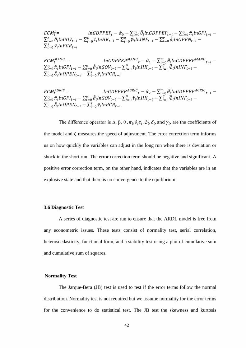
42
𝐸𝐶𝑀𝑡𝐿= 𝑙𝑛𝐺𝐷𝑃𝑃𝐸𝑃𝑡 − �̂�0 − ∑ 𝜃𝑖𝑙𝑛𝐺𝐷𝑃𝑃𝐸𝑃𝑡−𝑖
𝑚𝑖=0 − ∑ �̂�𝑖𝑙𝑛𝐺𝐹𝐼𝑡−𝑖
𝑛𝑖=0 −
∑ �̂�𝑖𝑙𝑛𝐺𝑂𝑉𝑡−𝑖𝑜𝑖=0 − ∑ �̂�𝑖𝑙𝑛𝐻𝐾𝑡−𝑖
𝑝𝑖=0 − ∑ ∅̂𝑖𝑙𝑛𝐼𝑁𝐹𝑡−𝑖
𝑞𝑖=0 − ∑ 𝛿𝑖𝑙𝑛𝑂𝑃𝐸𝑁𝑡−𝑖
𝑟𝑖=0 −
∑ 𝛾𝑖𝑙𝑛𝑃𝐺𝑅𝑡−𝑖𝑠𝑖=0
𝐸𝐶𝑀𝑡𝑀𝐴𝑁𝑈= 𝑙𝑛𝐺𝐷𝑃𝑃𝐸𝑃𝑀𝐴𝑁𝑈
𝑡 − �̂�1 − ∑ 𝜃𝑖𝑙𝑛𝐺𝐷𝑃𝑃𝐸𝑃𝑀𝐴𝑁𝑈𝑡−𝑖
𝑚𝑖=0 −
∑ �̂�𝑖𝑙𝑛𝐺𝐹𝐼𝑡−𝑖𝑛𝑖=0 − ∑ �̂�𝑖𝑙𝑛𝐺𝑂𝑉𝑡−𝑖
𝑜𝑖=0 − ∑ �̂�𝑖𝑙𝑛𝐻𝐾𝑡−𝑖
𝑝𝑖=0 − ∑ ∅̂𝑖𝑙𝑛𝐼𝑁𝐹𝑡−𝑖
𝑞𝑖=0 −
∑ 𝛿𝑖𝑙𝑛𝑂𝑃𝐸𝑁𝑡−𝑖𝑟𝑖=0 − ∑ 𝛾𝑖𝑙𝑛𝑃𝐺𝑅𝑡−𝑖
𝑠𝑖=0
𝐸𝐶𝑀𝑡𝐴𝐺𝑅𝐼𝐶= 𝑙𝑛𝐺𝐷𝑃𝑃𝐸𝑃𝐴𝐺𝑅𝐼𝐶
𝑡 − �̂�2 − ∑ 𝜃𝑖𝑙𝑛𝐺𝐷𝑃𝑃𝐸𝑃𝐴𝐺𝑅𝐼𝐶𝑡−𝑖
𝑚𝑖=0 −
∑ �̂�𝑖𝑙𝑛𝐺𝐹𝐼𝑡−𝑖𝑛𝑖=0 − ∑ �̂�𝑖𝑙𝑛𝐺𝑂𝑉𝑡−𝑖
𝑜𝑖=0 − ∑ �̂�𝑖𝑙𝑛𝐻𝐾𝑡−𝑖
𝑝𝑖=0 − ∑ ∅̂𝑖𝑙𝑛𝐼𝑁𝐹𝑡−𝑖
𝑞𝑖=0 −
∑ 𝛿𝑖𝑙𝑛𝑂𝑃𝐸𝑁𝑡−𝑖𝑟𝑖=0 − ∑ 𝛾𝑖𝑙𝑛𝑃𝐺𝑅𝑡−𝑖
𝑠𝑖=0
The difference operator is ∆, β, θ , 𝜋𝑖,𝜗𝑖𝜏𝑖 , ∅𝑖, 𝛿𝑖, and 𝛾𝑖, are the coefficients of
the model and 휁 measures the speed of adjustment. The error correction term informs
us on how quickly the variables can adjust in the long run when there is deviation or
shock in the short run. The error correction term should be negative and significant. A
positive error correction term, on the other hand, indicates that the variables are in an
explosive state and that there is no convergence to the equilibrium.
3.6 Diagnostic Test
A series of diagnostic test are run to ensure that the ARDL model is free from
any econometric issues. These tests consist of normality test, serial correlation,
heteroscedasticity, functional form, and a stability test using a plot of cumulative sum
and cumulative sum of squares.
Normality Test
The Jarque-Bera (JB) test is used to test if the error terms follow the normal
distribution. Normality test is not required but we assume normality for the error terms
for the convenience to do statistical test. The JB test the skewness and kurtosis
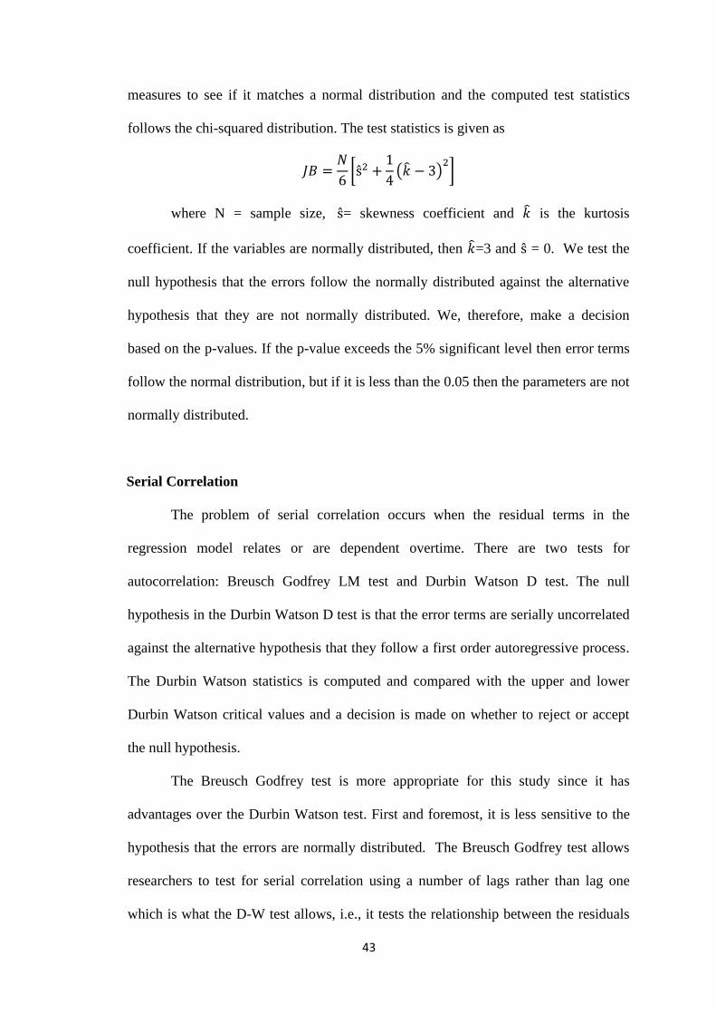
43
measures to see if it matches a normal distribution and the computed test statistics
follows the chi-squared distribution. The test statistics is given as
𝐽𝐵 =𝑁
6[ŝ2 +
1
4(�̂� − 3)
2]
where N = sample size, ŝ= skewness coefficient and �̂� is the kurtosis
coefficient. If the variables are normally distributed, then �̂�=3 and ŝ = 0. We test the
null hypothesis that the errors follow the normally distributed against the alternative
hypothesis that they are not normally distributed. We, therefore, make a decision
based on the p-values. If the p-value exceeds the 5% significant level then error terms
follow the normal distribution, but if it is less than the 0.05 then the parameters are not
normally distributed.
Serial Correlation
The problem of serial correlation occurs when the residual terms in the
regression model relates or are dependent overtime. There are two tests for
autocorrelation: Breusch Godfrey LM test and Durbin Watson D test. The null
hypothesis in the Durbin Watson D test is that the error terms are serially uncorrelated
against the alternative hypothesis that they follow a first order autoregressive process.
The Durbin Watson statistics is computed and compared with the upper and lower
Durbin Watson critical values and a decision is made on whether to reject or accept
the null hypothesis.
The Breusch Godfrey test is more appropriate for this study since it has
advantages over the Durbin Watson test. First and foremost, it is less sensitive to the
hypothesis that the errors are normally distributed. The Breusch Godfrey test allows
researchers to test for serial correlation using a number of lags rather than lag one
which is what the D-W test allows, i.e., it tests the relationship between the residuals
44
with time t and t-k, where k is the number of lags. The null hypothesis states that there
is no serial correlation between the error terms against the alternative hypothesis that
serial correlation is present. An LM test which is converted to an F-test is computed to
make a decision and if the p-value is greater than 5% the null hypothesis is rejected,
meaning that there is no serial correlation between the residuals in the model.
Alternatively, if the p-value is less than 5% then the problem of serial correlation
exists.
Heteroscedasticity
The Breusch Pagan test for heteroscedasticity is used for the study. This is
used to test for heteroscedasticity in a linear regression model, with the null
hypothesis that the variance of the errors are equal as against the alternative
hypothesis that they are not equal. The test follows the chi-squared distribution such
that if the test statistics has a p-value lower than the threshold of 5%, the null
hypothesis is rejected i.e., heteroscedasticity exists. We fail to reject the null
hypothesis if the test statistics have a p-value greater than 5% significance level,
implying that no heteroscedasticity exists.
The conditional heteroscedasticity in the residual terms is examined using the
Autoregressive Conditional Heteroscedasticity (ARCH) test in this study. The ARCH
test is a regression of the squared residuals on a constant and lagged residuals. The
computed F-statistics from this test follows a chi-squared distribution and the null
hypothesis is that there is no conditional heteroscedasticity against the alternative
hypothesis that the ARCH model describes the series. We fail to reject the null
hypothesis that if the p-value is greater than the 5% significance levels but if the p-
value is less than the 5% significance levels then the null hypothesis is rejected.
45
Functional Form
One of the basic problems in econometrics is model misspecification. The
Ramsey RESET test is used to detect misspecifications like incorrect functional form
(i.e., when some or all of the series are log transformed, or whether the powers of the
fitted values of the dependent variable have any power in describing the dependent
variable this can occur), measurement errors (which occur when the residual terms and
the independent and values of the lagged dependent variables are correlated), and
omitted variables. It simply tests if the functional form of the short-run model is
appropriately specified. The regression equation is specified as follows:
�̂� = 𝐸{𝑦I𝑥} = �̂�𝑥
Ramsey’s test tests whether �̂�𝑥, (�̂�𝑥)2, … , (�̂�𝑥)𝑘 has any power in explaining
𝑦. This is done by estimating the following regression
𝑦 = 𝛼𝑥 + 𝜏1�̂�2 + ⋯ + 𝜏𝑘−1�̂�𝑘 + 휀
The null hypothesis is 𝐻0: 𝜏1 = 𝜏2 = ⋯ = 𝜏𝑘−1 = 0 againt the alternative
𝐻1: 𝜏1 ≠ 𝜏2 ≠ ⋯ . ≠ 𝜏𝑘−1. A significant F-test statistic where the p-value is less than
the 5% significance levels (i.e., rejection of H0) means that the model suffers from
specification error. Otherwise, the model is correctly specified.
Stability Test
According to Pesaran, et al. (2001) it is important to check for the stability of
the parameters. Following Pesaran, et al. (2001), we use the cumulative sum
(CUSUM) and the cumulative sum squared (CUSUMSQ) to test for the stability of the
long run and short run parameters. The null hypothesis is all the parameters in the
model are stable and the alternative hypothesis is that the parameters are not stable.
The CUSUM and CUSMSQ tests substantially test for structural breaks and are
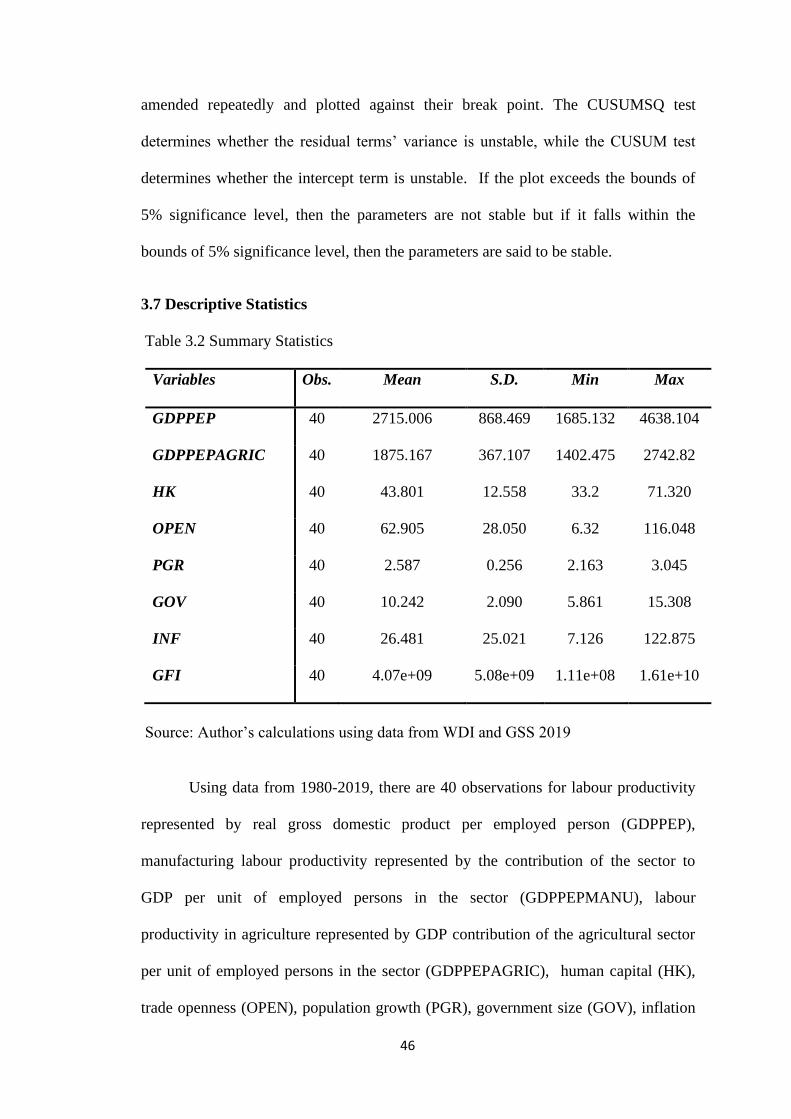
46
amended repeatedly and plotted against their break point. The CUSUMSQ test
determines whether the residual terms’ variance is unstable, while the CUSUM test
determines whether the intercept term is unstable. If the plot exceeds the bounds of
5% significance level, then the parameters are not stable but if it falls within the
bounds of 5% significance level, then the parameters are said to be stable.
3.7 Descriptive Statistics
Table 3.2 Summary Statistics
Variables Obs. Mean S.D. Min Max
GDPPEP 40 2715.006 868.469 1685.132 4638.104
GDPPEPAGRIC 40 1875.167 367.107 1402.475 2742.82
HK 40 43.801 12.558 33.2 71.320
OPEN 40 62.905 28.050 6.32 116.048
PGR 40 2.587 0.256 2.163 3.045
GOV 40 10.242 2.090 5.861 15.308
INF 40 26.481 25.021 7.126 122.875
GFI 40 4.07e+09 5.08e+09 1.11e+08 1.61e+10
Source: Author’s calculations using data from WDI and GSS 2019
Using data from 1980-2019, there are 40 observations for labour productivity
represented by real gross domestic product per employed person (GDPPEP),
manufacturing labour productivity represented by the contribution of the sector to
GDP per unit of employed persons in the sector (GDPPEPMANU), labour
productivity in agriculture represented by GDP contribution of the agricultural sector
per unit of employed persons in the sector (GDPPEPAGRIC), human capital (HK),
trade openness (OPEN), population growth (PGR), government size (GOV), inflation
47
(INF), and gross fixed investment (GFI). The result from Table 3.2 shows that the
average labour productivity measured as real GDP per employed person is around
USD 2,715 for the period under study. It reached its minimum (USD1685.13) in 1983
when Ghana recorded its worst post-independence recession and peaked around 2019.
Labour productivity grew steadily at 1.5 percent in the period. Population growth
(PGR) was very stable throughout the period averaging around 2.59% annually. The
lowest population growth rate was recorded in 2019 (2.16%). It can partly be
attributed to increased sex education and the use of contraceptives. Another key
explanatory variable for the study is inflation (INF). It averaged around 26.48%,
indicating that the general price levels were increasing at a rate above the Bank of
Ghana’s medium-term inflation target of 8% +/-2 percentage points in 2002.
Human capital (HK), as measured by the gross enrollment in secondary school,
and averaged 43.80% over the period. This means that two out of every five children
aged between 15 and 19 years were enrolled in secondary school from 1980 to 2019.
Gross enrollment was lowest in 1991 when it was 33.2% but has since grown steadily
and reached a record high in 2018 (71.32%). The recent high enrollment from 2017 is
partly attributed to the free secondary school policy that absorbs all fees of every
Ghanaian child attending public high school. The sum of Ghana's export and import
volumes as a percentage of GDP (OPEN) averaged 62.91% annually. The average
government size (GOV) was 10.24% of GDP. The government size has a direct
impact on the government's fiscal position and leads to excessive borrowing since
government revenue is way below its planned expenditure, but between 1986-1989
were the only years when the government of Ghana achieved a budget surplus. It can
be observed that in the years 1992, 2004, 2008 and 2012, government size increased
considerably because of the elections in those years. In 2011, expenditure of
48
government as a proportion of GDP rose to 13.79% from the previous year's 7.07%.
This was partly due to the implementation of the Single Spine Pay Structure (SSPS).
The SSPS was introduced to compensate workers in the public sector with comparable
qualifications as those in the private sector who received higher salary (Ampofo and
Tchatoka, 2019). Between 2010 when the policy was rolled-out to 2012, public sector
expenditure on salaries increased from USD 343 million to USD 1.2 billion by the end
of 2012.The average annual addition to capital stock over the period stood at USD
4.07 billion over the period. The minimum gross fixed investment (GFI) was recorded
in the year 1981 and was USD 110.59 million. The maximum gross fixed investment
between 1980-2019 was USD 16.07 billion, which was recorded in 2013.
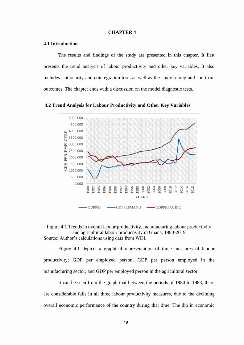
49
CHAPTER 4
4.1 Introduction
The results and findings of the study are presented in this chapter. It first
presents the trend analysis of labour productivity and other key variables. It also
includes stationarity and cointegration tests as well as the study’s long and short-run
outcomes. The chapter ends with a discussion on the model diagnostic tests.
4.2 Trend Analysis for Labour Productivity and Other Key Variables
Figure 4.1 Trends in overall labour productivity, manufacturing labour productivity
and agricultural labour productivity in Ghana, 1980-2019
Source: Author’s calculations using data from WDI.
Figure 4.1 depicts a graphical representation of three measures of labour
productivity; GDP per employed person, GDP per person employed in the
manufacturing sector, and GDP per employed person in the agricultural sector.
It can be seen from the graph that between the periods of 1980 to 1983, there
are considerable falls in all three labour productivity measures, due to the declining
overall economic performance of the country during that time. The dip in economic
0.000
500.000
1000.000
1500.000
2000.000
2500.000
3000.000
3500.000
4000.000
4500.000
5000.000
19
80
19
82
19
84
19
86
19
88
19
90
19
92
19
94
19
96
19
98
20
00
20
02
20
04
20
06
20
08
20
10
20
12
20
14
20
16
20
18
GD
P
PE
R E
MP
LO
YE
E
YEARS
GDPPEP GDPPEPMANU GDPPEPAGRIC
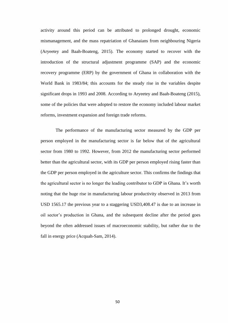
50
activity around this period can be attributed to prolonged drought, economic
mismanagement, and the mass repatriation of Ghanaians from neighbouring Nigeria
(Aryeetey and Baah-Boateng, 2015). The economy started to recover with the
introduction of the structural adjustment programme (SAP) and the economic
recovery programme (ERP) by the government of Ghana in collaboration with the
World Bank in 1983/84; this accounts for the steady rise in the variables despite
significant drops in 1993 and 2008. According to Aryeetey and Baah-Boateng (2015),
some of the policies that were adopted to restore the economy included labour market
reforms, investment expansion and foreign trade reforms.
The performance of the manufacturing sector measured by the GDP per
person employed in the manufacturing sector is far below that of the agricultural
sector from 1980 to 1992. However, from 2012 the manufacturing sector performed
better than the agricultural sector, with its GDP per person employed rising faster than
the GDP per person employed in the agriculture sector. This confirms the findings that
the agricultural sector is no longer the leading contributor to GDP in Ghana. It’s worth
noting that the huge rise in manufacturing labour productivity observed in 2013 from
USD 1565.17 the previous year to a staggering USD3,408.47 is due to an increase in
oil sector’s production in Ghana, and the subsequent decline after the period goes
beyond the often addressed issues of macroeconomic stability, but rather due to the
fall in energy price (Acquah-Sam, 2014).
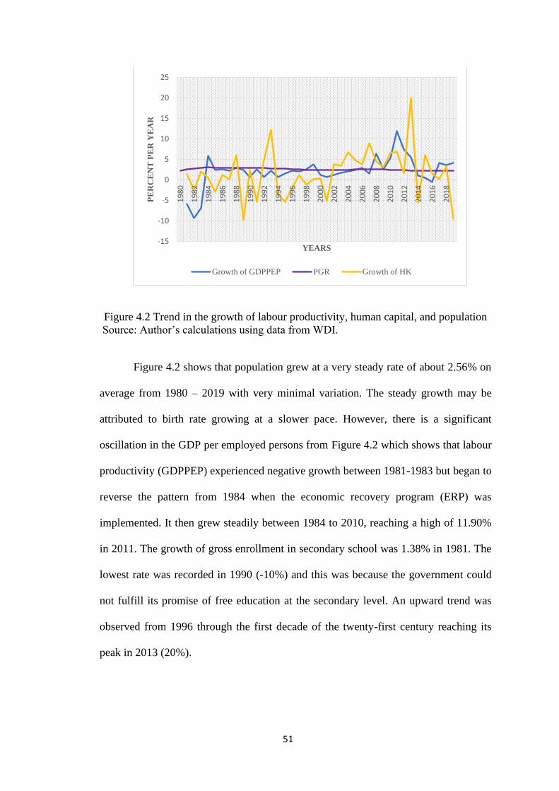
51
Figure 4.2 Trend in the growth of labour productivity, human capital, and population
Source: Author’s calculations using data from WDI.
Figure 4.2 shows that population grew at a very steady rate of about 2.56% on
average from 1980 – 2019 with very minimal variation. The steady growth may be
attributed to birth rate growing at a slower pace. However, there is a significant
oscillation in the GDP per employed persons from Figure 4.2 which shows that labour
productivity (GDPPEP) experienced negative growth between 1981-1983 but began to
reverse the pattern from 1984 when the economic recovery program (ERP) was
implemented. It then grew steadily between 1984 to 2010, reaching a high of 11.90%
in 2011. The growth of gross enrollment in secondary school was 1.38% in 1981. The
lowest rate was recorded in 1990 (-10%) and this was because the government could
not fulfill its promise of free education at the secondary level. An upward trend was
observed from 1996 through the first decade of the twenty-first century reaching its
peak in 2013 (20%).
-15
-10
-5
0
5
10
15
20
25
19
80
19
82
19
84
19
86
19
88
19
90
19
92
19
94
19
96
19
98
20
00
20
02
20
04
20
06
20
08
20
10
20
12
20
14
20
16
20
18
PE
RC
EN
T P
ER
YE
AR
YEARS
Growth of GDPPEP PGR Growth of HK
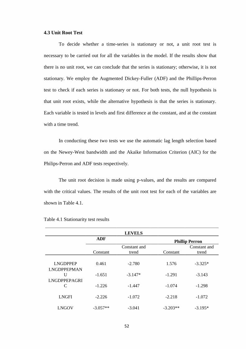
52
4.3 Unit Root Test
To decide whether a time-series is stationary or not, a unit root test is
necessary to be carried out for all the variables in the model. If the results show that
there is no unit root, we can conclude that the series is stationary; otherwise, it is not
stationary. We employ the Augmented Dickey-Fuller (ADF) and the Phillips-Perron
test to check if each series is stationary or not. For both tests, the null hypothesis is
that unit root exists, while the alternative hypothesis is that the series is stationary.
Each variable is tested in levels and first difference at the constant, and at the constant
with a time trend.
In conducting these two tests we use the automatic lag length selection based
on the Newey-West bandwidth and the Akaike Information Criterion (AIC) for the
Philips-Perron and ADF tests respectively.
The unit root decision is made using p-values, and the results are compared
with the critical values. The results of the unit root test for each of the variables are
shown in Table 4.1.
Table 4.1 Stationarity test results
LEVELS
ADF
Phillip Perron
Constant Constant and
trend Constant Constant and
trend
LNGDPPEP
0.461 -2.780 1.576 -3.325*
LNGDPPEPMAN
U
-1.651 -3.147* -1.291 -3.143
LNGDPPEPAGRI
C
-1.226 -1.447 -1.074 -1.298
LNGFI
-2.226 -1.072 -2.218 -1.072
LNGOV
-3.057** -3.041 -3.203** -3.195*

53
LNHK
0.225 -1.504 0.177 -1.479
LNINF
-1.022 -6.038*** -3.308** -5.485***
LNOPEN
-1.698
-1.366 -1.688 -1.424
LNPGR
-0.147
-4.151** -1.268 -5.102***
FIRST DIFFERENCE
ADF
Phillips-Perron
Constant Constant and
trend Constant Constant and
trend
LNGDPPEP -3.544** -3.722** -3.383** -3.465*
LNGDPPEPMAN
U -5.138*** -5.063*** -8.801*** -10.163***
LNGDPPEPAGRI
C -4.754*** -4.290*** -4.665*** -8.788***
LNGFI -3.081** -3.448* -3.054** -3.433*
LNGOV -5.104*** -3.180* -7.739*** -8.286***
LNHK -6.315*** -6.660*** -6.396*** -6.670***
LNINF -5.636*** -5.548*** -18.359*** -17.669*** LNOPEN -6.201*** -8.034*** -5.195*** -5.615***
LNPGR -4.491*** -4.400*** -5.641*** -4.922*** Note: ***, ** and * represent statistical significance at 1%, 5% and 10% levels,
respectively. The test statistics were compared with the Dickey-Fuller critical values. For
the regression with constant, the critical values are -2.608, -2.939, and -3.610 for 0.1, 0.05,
and 0.01 significance levels respectively. For the regression with a constant and trend terms,
the critical values are -3.196, -3.530, and -4.212 respectively.
Source: Author’s calculations.
Since both the PP and ADF test values are greater than the critical values
at 5% significance levels, the findings from the PP and ADF test for the variables
in Table 4.1 suggest that some of the variables are stationary at the levels. Also,
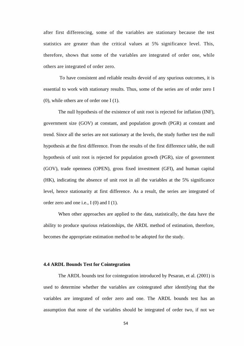
54
after first differencing, some of the variables are stationary because the test
statistics are greater than the critical values at 5% significance level. This,
therefore, shows that some of the variables are integrated of order one, while
others are integrated of order zero.
To have consistent and reliable results devoid of any spurious outcomes, it is
essential to work with stationary results. Thus, some of the series are of order zero I
(0), while others are of order one I (1).
The null hypothesis of the existence of unit root is rejected for inflation (INF),
government size (GOV) at constant, and population growth (PGR) at constant and
trend. Since all the series are not stationary at the levels, the study further test the null
hypothesis at the first difference. From the results of the first difference table, the null
hypothesis of unit root is rejected for population growth (PGR), size of government
(GOV), trade openness (OPEN), gross fixed investment (GFI), and human capital
(HK), indicating the absence of unit root in all the variables at the 5% significance
level, hence stationarity at first difference. As a result, the series are integrated of
order zero and one i.e., I (0) and I (1).
When other approaches are applied to the data, statistically, the data have the
ability to produce spurious relationships, the ARDL method of estimation, therefore,
becomes the appropriate estimation method to be adopted for the study.
4.4 ARDL Bounds Test for Cointegration
The ARDL bounds test for cointegration introduced by Pesaran, et al. (2001) is
used to determine whether the variables are cointegrated after identifying that the
variables are integrated of order zero and one. The ARDL bounds test has an
assumption that none of the variables should be integrated of order two, if not we
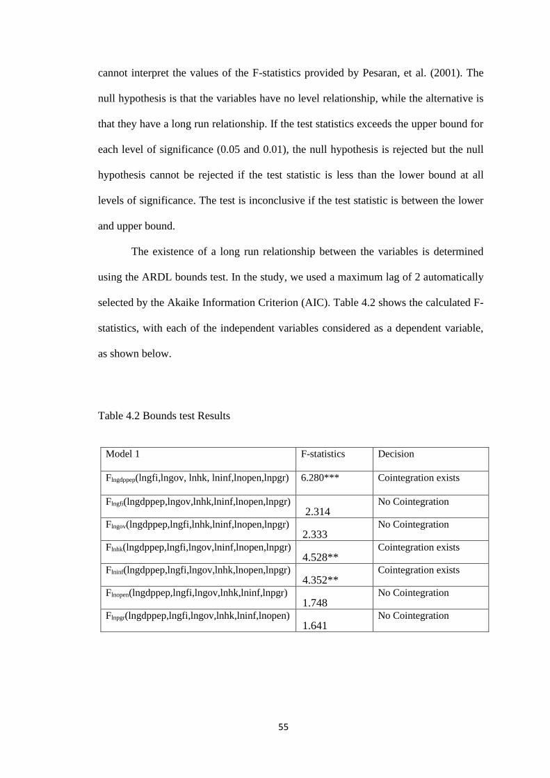
55
cannot interpret the values of the F-statistics provided by Pesaran, et al. (2001). The
null hypothesis is that the variables have no level relationship, while the alternative is
that they have a long run relationship. If the test statistics exceeds the upper bound for
each level of significance (0.05 and 0.01), the null hypothesis is rejected but the null
hypothesis cannot be rejected if the test statistic is less than the lower bound at all
levels of significance. The test is inconclusive if the test statistic is between the lower
and upper bound.
The existence of a long run relationship between the variables is determined
using the ARDL bounds test. In the study, we used a maximum lag of 2 automatically
selected by the Akaike Information Criterion (AIC). Table 4.2 shows the calculated F-
statistics, with each of the independent variables considered as a dependent variable,
as shown below.
Table 4.2 Bounds test Results
Model 1
F-statistics Decision
Flngdppep(lngfi,lngov, lnhk, lninf,lnopen,lnpgr) 6.280***
Cointegration exists
Flngfi(lngdppep,lngov,lnhk,lninf,lnopen,lnpgr)
2.314
No Cointegration
Flngov(lngdppep,lngfi,lnhk,lninf,lnopen,lnpgr)
2.333
No Cointegration
Flnhk(lngdppep,lngfi,lngov,lninf,lnopen,lnpgr)
4.528**
Cointegration exists
Flninf(lngdppep,lngfi,lngov,lnhk,lnopen,lnpgr)
4.352**
Cointegration exists
Flnopen(lngdppep,lngfi,lngov,lnhk,lninf,lnpgr)
1.748
No Cointegration
Flnpgr(lngdppep,lngfi,lngov,lnhk,lninf,lnopen)
1.641
No Cointegration
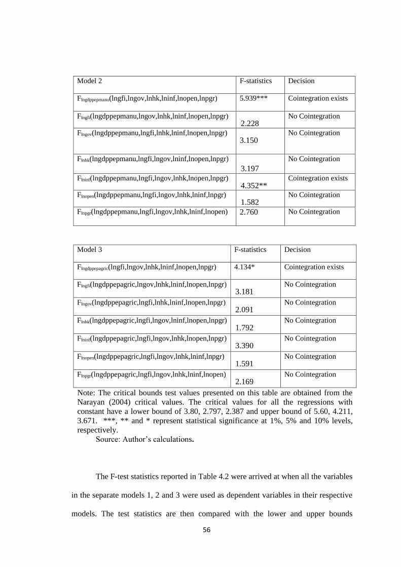
56
Model 2
F-statistics Decision
Flngdppepmanu(lngfi,lngov,lnhk,lninf,lnopen,lnpgr)
5.939*** Cointegration exists
Flngfi(lngdppepmanu,lngov,lnhk,lninf,lnopen,lnpgr)
2.228
No Cointegration
Flngov(lngdppepmanu,lngfi,lnhk,lninf,lnopen,lnpgr)
3.150
No Cointegration
Flnhk(lngdppepmanu,lngfi,lngov,lninf,lnopen,lnpgr)
3.197
No Cointegration
Flninf(lngdppepmanu,lngfi,lngov,lnhk,lnopen,lnpgr)
4.352**
Cointegration exists
Flnopen(lngdppepmanu,lngfi,lngov,lnhk,lninf,lnpgr)
1.582
No Cointegration
Flnpgr(lngdppepmanu,lngfi,lngov,lnhk,lninf,lnopen) 2.760
No Cointegration
Model 3 F-statistics Decision
Flngdppepagric(lngfi,lngov,lnhk,lninf,lnopen,lnpgr) 4.134* Cointegration exists
Flngfi(lngdppepagric,lngov,lnhk,lninf,lnopen,lnpgr)
3.181
No Cointegration
Flngov(lngdppepagric,lngfi,lnhk,lninf,lnopen,lnpgr)
2.091
No Cointegration
Flnhk(lngdppepagric,lngfi,lngov,lninf,lnopen,lnpgr)
1.792
No Cointegration
Flninf(lngdppepagric,lngfi,lngov,lnhk,lnopen,lnpgr)
3.390
No Cointegration
Flnopen(lngdppepagric,lngfi,lngov,lnhk,lninf,lnpgr)
1.591
No Cointegration
Flnpgr(lngdppepagric,lngfi,lngov,lnhk,lninf,lnopen)
2.169
No Cointegration
Note: The critical bounds test values presented on this table are obtained from the
Narayan (2004) critical values. The critical values for all the regressions with
constant have a lower bound of 3.80, 2.797, 2.387 and upper bound of 5.60, 4.211,
3.671. ***, ** and * represent statistical significance at 1%, 5% and 10% levels,
respectively.
Source: Author’s calculations.
The F-test statistics reported in Table 4.2 were arrived at when all the variables
in the separate models 1, 2 and 3 were used as dependent variables in their respective
models. The test statistics are then compared with the lower and upper bounds
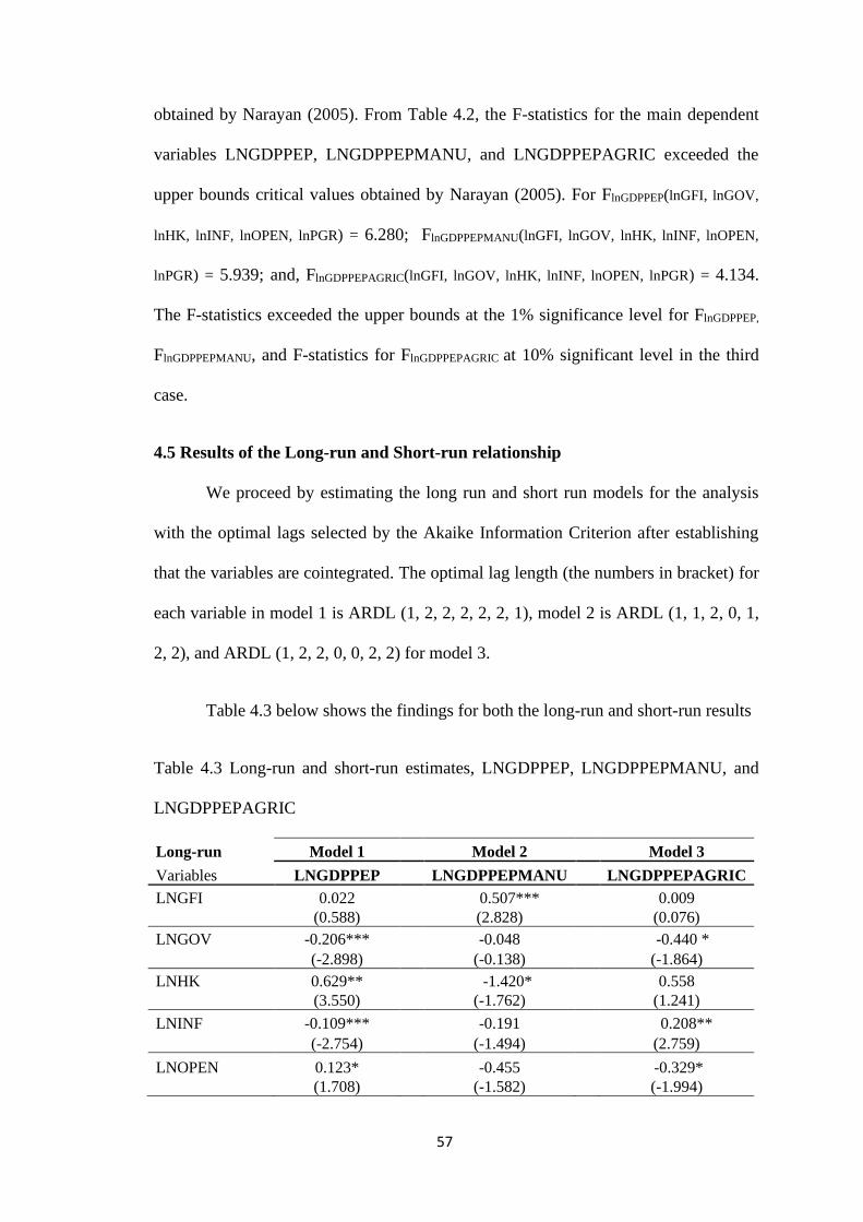
57
obtained by Narayan (2005). From Table 4.2, the F-statistics for the main dependent
variables LNGDPPEP, LNGDPPEPMANU, and LNGDPPEPAGRIC exceeded the
upper bounds critical values obtained by Narayan (2005). For FlnGDPPEP(lnGFI, lnGOV,
lnHK, lnINF, lnOPEN, lnPGR) = 6.280; FlnGDPPEPMANU(lnGFI, lnGOV, lnHK, lnINF, lnOPEN,
lnPGR) = 5.939; and, FlnGDPPEPAGRIC(lnGFI, lnGOV, lnHK, lnINF, lnOPEN, lnPGR) = 4.134.
The F-statistics exceeded the upper bounds at the 1% significance level for FlnGDPPEP,
FlnGDPPEPMANU, and F-statistics for FlnGDPPEPAGRIC at 10% significant level in the third
case.
4.5 Results of the Long-run and Short-run relationship
We proceed by estimating the long run and short run models for the analysis
with the optimal lags selected by the Akaike Information Criterion after establishing
that the variables are cointegrated. The optimal lag length (the numbers in bracket) for
each variable in model 1 is ARDL (1, 2, 2, 2, 2, 2, 1), model 2 is ARDL (1, 1, 2, 0, 1,
2, 2), and ARDL (1, 2, 2, 0, 0, 2, 2) for model 3.
Table 4.3 below shows the findings for both the long-run and short-run results
Table 4.3 Long-run and short-run estimates, LNGDPPEP, LNGDPPEPMANU, and
LNGDPPEPAGRIC
Long-run Model 1 Model 2 Model 3
Variables LNGDPPEP LNGDPPEPMANU LNGDPPEPAGRIC
LNGFI 0.022 0.507*** 0.009
(0.588) (2.828) (0.076)
LNGOV -0.206*** -0.048 -0.440 *
(-2.898) (-0.138) (-1.864)
LNHK 0.629** -1.420* 0.558
(3.550) (-1.762) (1.241)
LNINF -0.109*** -0.191 0.208**
(-2.754) (-1.494) (2.759)
LNOPEN 0.123* -0.455 -0.329*
(1.708) (-1.582) (-1.994)
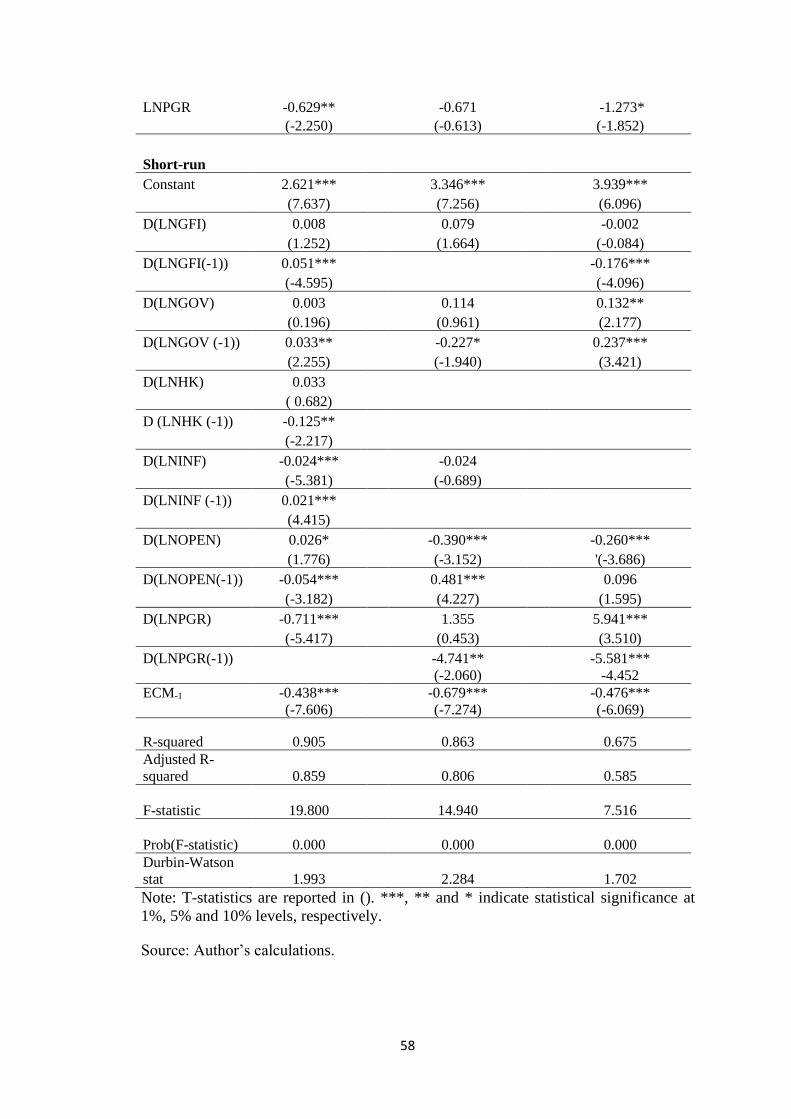
58
LNPGR -0.629** -0.671 -1.273*
(-2.250) (-0.613) (-1.852)
Short-run
Constant 2.621*** 3.346*** 3.939***
(7.637) (7.256) (6.096)
D(LNGFI) 0.008 0.079 -0.002
(1.252) (1.664) (-0.084)
D(LNGFI(-1)) 0.051*** -0.176***
(-4.595) (-4.096)
D(LNGOV) 0.003 0.114 0.132**
(0.196) (0.961) (2.177)
D(LNGOV (-1)) 0.033** -0.227* 0.237***
(2.255) (-1.940) (3.421)
D(LNHK) 0.033 ( 0.682)
D (LNHK (-1)) -0.125** (-2.217)
D(LNINF) -0.024*** -0.024 (-5.381) (-0.689)
D(LNINF (-1)) 0.021*** (4.415)
D(LNOPEN) 0.026* -0.390*** -0.260***
(1.776) (-3.152) '(-3.686)
D(LNOPEN(-1)) -0.054*** 0.481*** 0.096
(-3.182) (4.227) (1.595)
D(LNPGR) -0.711*** 1.355 5.941***
(-5.417) (0.453) (3.510)
D(LNPGR(-1)) -4.741** -5.581***
(-2.060) -4.452
ECM-1 -0.438*** -0.679*** -0.476***
(-7.606) (-7.274) (-6.069)
R-squared 0.905 0.863 0.675
Adjusted R-
squared 0.859 0.806 0.585
F-statistic 19.800
14.940 7.516
Prob(F-statistic) 0.000
0.000 0.000
Durbin-Watson
stat 1.993 2.284 1.702
Note: T-statistics are reported in (). ***, ** and * indicate statistical significance at
1%, 5% and 10% levels, respectively.
Source: Author’s calculations.
59
4.5.1 Analysis of the Long and Short-run Estimates
4.5.1.1 Labour Productivity (Overall)
Table 4.3 shows that a 1% rise in population growth is linked to a 0.63% fall in
overall labour productivity, which is statistically significant at 5%. This shows that as
the population increases, it reduces the overall productivity of labour in the economy
of Ghana. This is consistent with the findings of Hamza (2015). Also, government size
is found to have a negative relationship with labour productivity. All other things
being equal, a 1% rise in government size is associated with a 0.21% decline in labour
productivity in the long run. The result is consistent with the findings of Dua and Garg
(2017), where they found a negative relationship between government spending and
labour productivity. But this finding contradicts with the findings of Awotunde (2018)
who showed that government spending that goes into labour issues increases labour
productivity significantly.
Again, from the estimation, a percentage increase in human capital will
increase on average the overall labour productivity by 0.63% in the long run, ceteris
paribus. At 5% significant level, this relationship is considered statistically significant.
This again, confirms our earlier supposition that labour productivity will increase with
an increase in enrollment of labour in secondary and tertiary schools. This result is in
line with previous studies by Dua and Garg (2017) and Samargandi (2018).
Also, if all other factors remain stable, a percentage rise in inflation will result
in a 0.11% decrease in labour productivity, on average. This was expected and
consistent with our initial hypothesis that inflation reduces labour productivity. It also
corresponds to Yildirim (2015) and Hondroyiannis and Papapetrou (1997) results.
They argued that inflation erodes nominal wages and makes the opportunity cost of
60
working less costly. It also distorts the market in the sense that investors are unable to
accurately predict price changes. At 1% significance level, this relationship is
statistically significant.
The coefficient of trade openness is positive as expected from our supposition.
It is statistically significant at t he 10% leve l . Specifically, the result shows that, if
trade openness increases, labour productivity will increase by 0.12%. This means that
increased trade openness is a factor influencing labour productivity in Ghana in the
long run. In fact, Ghana has trade relations, especially in the export of cocoa, timber,
mineral fuels and precious metals. Since the mid-1980s, when import substitution
policies were relaxed, imports have increased. As a result, Ghana’s trade liberation
policies have produced positive results. Hence, the positive relationship between trade
openness and labour productivity supports this finding and also consistent with
previous research in Ghana (Abosi, 2008; Djokoto, 2012). With gross fixed
investment, no statistically significant relationship exists with labour productivity in
the long-run.
The error correction term (ECM-1) refers to how easily the dependent variable
reacts to changes in the independent variables before settling into its long run
equilibrium level. The negative and significant ecm term shows how the adjustment
process is effective and able to restore to equilibrium. An error correction term of -
0.44 in the first model shows that any disequilibrium will be corrected within a year at
a speed of approximately 44%.
The first lag of GFI is found to have a substantial positive effect on labour
productivity. If gross fixed investment in the previous year increases by 1%, there will
be a 0.05% rise in the overall labour productivity in the current year and this is
61
significant at the 0.01 significance level. Government spending is found to be
insignificant but the first lag is significant at 5%, and it has a positive effect on labour
productivity. This means that a 1% increase in the previous year government spending
is related to a 0.03% increase in overall labour productivity. This contradicts the long-
run coefficient.
Also, a 1% rise in human capital in the previous year will lead to a 0.13%,
decrease in labour productivity, holding other variables constant. Human capital in the
current year indicates a positive relationship on labour productivity by 0.03% but this
is statistically insignificant. This is in line with the long-run estimate and a study by
Dua and Garg who used the same indicator, enrollment in secondary school as we
used but the only difference is that it is statistically not significant.
The study also found that a percentage increase in inflation rate is associated
with a 0.024% fall on labour productivity in the economy. This conforms to the long-
run estimate and shows that rising prices has the tendency of reducing labour
productivity since it reduces the purchasing power of labour. However, the first lag of
inflation rate shows a positive impact on labour productivity by 0.021%, all other
things being equal, and it is statistically significant.
Finally, population growth and the first lag of trade openness were all found to
have a significantly negative impact on labour productivity in the short run. With trade
openness, the effect is minimal on labour productivity with an elasticity value of
approximately -0.05.
62
4.5.1.2 Manufacturing Labour Productivity
At a 1% significance level, a percentage rise in gross fixed investment is
associated with a 0.51% increase in manufacturing labour productivity in the long run,
all other things held constant. This means that increasing capital investment will
improve labour productivity in the manufacturing sector in the long run, resulting in
overall economic growth. Also, a 1% increase in gross enrollment is associated with a
1.42% fall in manufacturing labour productivity. Theoretically, an investment in
human capital in an economy improves labour productivity, the empirical evidence is
somewhat mixed especially with developing countries. The relationship is only
significant at the 10% significance level. The coefficients of population growth,
government size, inflation, and trade openness are all negative and statistically
insignificant.
The error correction term has a coefficient of -0.679 and this means that in the
current year, roughly 68% of the previous year’s disequilibrium will return to long run
equilibrium. Trade openness and its first lag have a significant impact on
manufacturing labour productivity in the short run. In the short run, an increase in
total imports and exports to GDP, as well as an increase in its first lag is associated
with a 0.39% fall and 0.48% increase in manufacturing labour productivity,
respectively. Population growth is statistically insignificant in the short run, but its
first lag is negatively linked to manufacturing labour productivity. With a 1% rise in
population is associated with a 4.74% decline in the sector’s productivity at 5%
significance level.
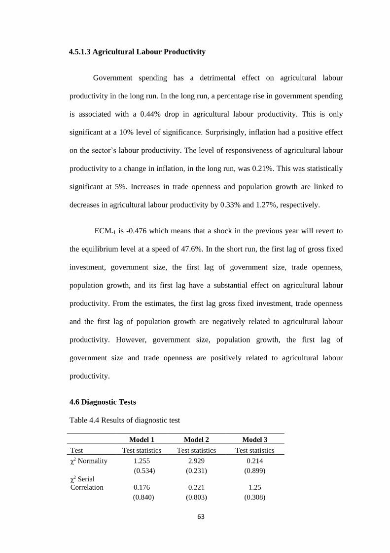
63
4.5.1.3 Agricultural Labour Productivity
Government spending has a detrimental effect on agricultural labour
productivity in the long run. In the long run, a percentage rise in government spending
is associated with a 0.44% drop in agricultural labour productivity. This is only
significant at a 10% level of significance. Surprisingly, inflation had a positive effect
on the sector’s labour productivity. The level of responsiveness of agricultural labour
productivity to a change in inflation, in the long run, was 0.21%. This was statistically
significant at 5%. Increases in trade openness and population growth are linked to
decreases in agricultural labour productivity by 0.33% and 1.27%, respectively.
ECM-1 is -0.476 which means that a shock in the previous year will revert to
the equilibrium level at a speed of 47.6%. In the short run, the first lag of gross fixed
investment, government size, the first lag of government size, trade openness,
population growth, and its first lag have a substantial effect on agricultural labour
productivity. From the estimates, the first lag gross fixed investment, trade openness
and the first lag of population growth are negatively related to agricultural labour
productivity. However, government size, population growth, the first lag of
government size and trade openness are positively related to agricultural labour
productivity.
4.6 Diagnostic Tests
Table 4.4 Results of diagnostic test
Model 1 Model 2 Model 3
Test Test statistics Test statistics Test statistics
ꭓ2 Normality 1.255 2.929 0.214
(0.534) (0.231) (0.899)
ꭓ2 Serial
Correlation 0.176 0.221 1.25
(0.840) (0.803) (0.308)
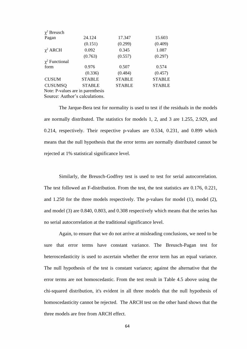
64
ꭓ2 Breusch
Pagan 24.124 17.347 15.603
(0.151) (0.299) (0.409)
ꭓ2 ARCH 0.092 0.345 1.087
(0.763) (0.557) (0.297)
ꭓ2 Functional
form 0.976 0.507 0.574
(0.336) (0.484) (0.457)
CUSUM STABLE STABLE STABLE
CUSUMSQ STABLE STABLE STABLE
Note: P-values are in parenthesis
Source: Author’s calculations.
The Jarque-Bera test for normality is used to test if the residuals in the models
are normally distributed. The statistics for models 1, 2, and 3 are 1.255, 2.929, and
0.214, respectively. Their respective p-values are 0.534, 0.231, and 0.899 which
means that the null hypothesis that the error terms are normally distributed cannot be
rejected at 1% statistical significance level.
Similarly, the Breusch-Godfrey test is used to test for serial autocorrelation.
The test followed an F-distribution. From the test, the test statistics are 0.176, 0.221,
and 1.250 for the three models respectively. The p-values for model (1), model (2),
and model (3) are 0.840, 0.803, and 0.308 respectively which means that the series has
no serial autocorrelation at the traditional significance level.
Again, to ensure that we do not arrive at misleading conclusions, we need to be
sure that error terms have constant variance. The Breusch-Pagan test for
heteroscedasticity is used to ascertain whether the error term has an equal variance.
The null hypothesis of the test is constant variance; against the alternative that the
error terms are not homoscedastic. From the test result in Table 4.5 above using the
chi-squared distribution, it's evident in all three models that the null hypothesis of
homoscedasticity cannot be rejected. The ARCH test on the other hand shows that the
three models are free from ARCH effect.
65
Also, Ramsey's RESET test is often used to ensure the functional form is
defined correctly. The null hypothesis of no omitted variable bias cannot be rejected at
5% significance level. Finally, we test whether the parameters are stable over time.
We used the cumulative sum (CUSUM) and the cumulative sum squared
(CUSUMSQ) to test if the parameters are stable, as suggested by Pesaran, et al.
(2001). The CUSUM and CUSUMSQ is presented in the Appendix and it shows that
at 95% confidence interval the parameters are stable over time in all the three models.
The main problem with the CUSUM and CUSUMSQ tests is that they have low
power of rejecting the null hypothesis, such that they only report the periods where
there is stability of the parameters in the model.

66
CHAPTER 5
5.1 Introduction
The study was carried out basically to assess the effect of population growth
on labour productivity as well as to ascertain the various determinants of total labour
productivity, labour productivity in the manufacturing and the agricultural sectors.
The chapter is made up of summary of the findings of the study, conclusion, and
recommendations for policy implementation.
5.2 Summary of Research Findings
The aim of this research was to look at the effect of population growth on
labour productivity, examine the trends in labour productivity, and assess what factors
are driving labour productivity across two sectors of the economy. The research used
the autoregressive distributed lag (ARDL) estimation method to analyze time-series
data from 1980–2019. The study commenced by looking at the trends in the
endogenous variables (i.e., labour productivity, and labour productivity within the
manufacturing, and agriculture sectors). The trend analysis did indicate that all three
variables had a positive trend over the period under consideration. To check the
accuracy of the estimation and to cure the model of any spurious outcomes, the PP and
ADF stationarity tests were carried out. These tests revealed that some of the variables
were stationary at levels or some were stationary at first difference. This formed the
basis for us to specify an ARDL model since it is most suitable for estimating
parameters that are a mixture of I (0) and I (1). The next step was to see if the
variables were cointegrated. Following Pesaran, et al. (2001), the bounds test result for
cointegration established a long-run association for the three dependent variables
employed in the models: GDPPEP, GDPPEPMANU and GDPPEPAGRIC. We then
estimated the long-run impacts and the error correction models related to the long-run
67
estimates. The various diagnostic tests did indicate that the models did not suffer from
serial autocorrelation, heteroscedasticity, or functional misspecification. The results of
the CUSUM and CUSUMSQ also indicate that the models were stable.
The study concludes that for the period between 1980 and 2019, Ghana's
overall labour productivity, as well as agriculture and manufacturing sectors labour
productivities have been increasing, which is an indication that the country's economic
policies over the years are gradually yielding positive results, at least on the labour
front. This is consistent with earlier works on the impact of economic growth in
Ghana (Aryeetey and Baah-Boateng, 2015). However, more work needs to be done to
sustain and even increase these gains.
The study also concludes that the main drivers of overall labour productivity in
Ghana are human capital, trade openness, and gross fixed investment. As expected,
the study revealed that population growth, government size, and inflation would
eventually serve as a disincentive for workers, thereby reducing labour productivity.
However, we found that the first lag of gross fixed investment and size of government
has a positive effect on labour productivity in the short run, while population growth
and its first lag has a negative impact.
The study found that the factors influencing labour productivity in the
agriculture sector vary from those influencing manufacturing sector’s labour
productivity. Gross fixed investment is found to be strongly linked to the
manufacturing labour productivity in the long run. The exact opposite is true for gross
enrollment in secondary schools and manufacturing labour productivity, although it
was significant at 10%. In the short run, its only trade openness, its first lag and
population growth that significantly impacted manufacturing labour productivity.
68
Finally, the analysis found a significant and negative association in the long
run between government size and agricultural labour productivity (GDPPEPAGRIC).
Inflation in the long run was positively related to agricultural labour productivity. The
first lag of gross fixed investment, government size, first lag of government size, trade
openness, the first lag population growth, and population growth all have a significant
impact on agricultural labour productivity in the short run.
5.3 Conclusion
The study primarily set out to look at the effect of population growth on labour
productivity and also to look at the various factors affecting labour productivity in the
manufacturing and agricultural sectors. The empirical evidence indicated that, in the
long run, increased population growth would hurt the Ghanaian economy’s overall
labour productivity. In the manufacturing sector, there was no evidence of a long run
relationship between population growth and labour productivity. Finally, the analysis
showed that a proportionate increase in population growth in the long run, would
affect agricultural labour productivity by more than proportionate decline.
5.4 Limitations of the Study
The main limitation of this study is the lack of data which restricted the choice
of proxy for human capital to be gross enrollment in secondary and tertiary schools.
Also, due to the unavailability of data for the agricultural and manufacturing sectors in
Ghana, we used the same data for gross fixed investment, human capital, and trade
openness for both sectors.
Also, in this study, labour productivity was measured by GDP per employed
persons, but this is not the only measure for labour productivity. Therefore, it is
69
recommended that future researchers identity other measures of labour productivity
and reliable data in this area of study.
5.5 Policy Recommendations
A sound and stable macroeconomic outlook benefits the economy, labour
productivity, and citizens’ well-being. The following suggestions are made based on
the study’s findings.
The government, through its agencies such as the Ghana Health Service
(GHS), the National Commission for Civic Education (NCCE), and the traditional
authorities, should increase it education on birth controls in Ghana as increased
population growth would have a negative effect on labour productivity in the long run,
lowering the standard of living of every Ghanaian.
The second recommendation the study makes is for the monetary authority in
Ghana (Bank of Ghana) to continue to pursue its inflation-targeting monetary policy.
The monetary policy must be kept reasonably tight to control liquidity in circulation.
This will stabilize prices and purge the country of the negative effect of accelerated
inflation.
Finally, any policy geared towards increasing enrollment in the secondary and
tertiary levels of education must be highly encouraged. Policies such as the
government’s free SHS recently introduced in 2017 must be given sustainable funding
so that the labour force will be more competent. This, as the study suggests, will boost
GDP per employed person in the country.
70
REFERENCES
Abdullah, N. H., Shamsuddin, A., Wahab, E., & Aziati, A. (2015). The relationship
between organizational culture and product innovativeness. Procedia-Social
and Behavioural Sciences, 129.
Abosi, E. N. (2008). Determinants of foreign direct investment in Ghana (1975-
2005). United Nations African Institute for Economic Development and
Planning, New York, United States).
Acquah-Sam, E. (2014). Economic effects of oil and gas production and management
on the Ghanaian economy. European Scientific Journal.
Aggrey, N., Luvanda, E. & Shitundu, J. (2010). Human capital and labour
productivity in East African manufacturing firms. Current Research Journal of
Economic Theory, 2(2), 48-54.
Agyapong F. O., Agyapong A., Poku K., (2017). Nexus between social capital and
performance of micro and small firms in an emerging economy: The mediating
role of innovation. Cogent Business & Management 4 (1), 1309784.
Akintunde, T. S., Olomola, P. A. & Oladeji , S. I. (2013). Population dynamics and
economic growth. Journal of Economics and Sustainable Development, 4(13),
148-157.
Amade, P., & Bakari, I. (2019). Impact of Population Growth on Economic Growth in
Africa: A Dynamic Panel Data Approach (1980 -2015)
Ampofo, A., & Tchatoka, F. D. (2019). Reducing public-private sector pay
differentials: The single spine pay policy as a natural experiment in Ghana.
Economic Inquiry, 57(1), 283-315.
Anyemedu, K. (1993). “The economic policies of the PNDC” in Gyimah Boadi, ed.,
Ghana Under PADC Rule. Dakar: CODESRIA, 13-47.
Aragon F., Rud J. P., (2011). Mining, pollution, and agricultural productivity:
evidence from Ghana. SFU Economics Department.
Aryeetey, E., & Baah-boateng, W. (2015). WIDER Working Paper 2015 / 140
Understanding Ghana’s growth success story and job creation challenges.
WIDERWorkingPaper2015/140,December,1.
https://www.brookings.edu/research/understanding-ghanas-growth-success-
story-and-job-creation-challenges.
Attar, A. A., Gupta, A. K., & Desai, D. B. (2012). A study of various factors affecting
labour productivity and methods to improve it. IOSR Journal of Mechanical
and Civil Engineering (IOSR-JMCE), 1(3), 11-14.
Awotunde, Ibukunoluwa (2018). Capital accumulation and labour productivity growth
in Nigeria. International Journal of Economics and Financial Research, 4(6),
171-179.
71
Azuh, D., Oluwatoyin, M. A., & Fagbeminiyi, F. F. (2016). The determinants of
population growth in Nigeria: A cointegration approach. The International
Journal of Humanities & Social Studies, 4(11), 38-44.
Banerji, A. & Dua, P. (2004). Does low inflation imply high productivity? Economic
Cycle Research Institute. ECRI, New York.
Becker, G. S. (1997). An economic analysis of fertility. In J. L. Simon (Ed.), The
Economics of Population: Key modern writings. 2, 403–425. Elgar Reference
Collection.
Bloom, D., Canning, D., & Sevilla, J. (2003). The debate over the effects of population
growth on economic growth. The Demographic Dividend: A New Perspective on
the Economic Consequences of Population Change 1-24. Santa Monica, CA;
Arlington, VA; Pittsburgh, PA:RANDCorporation.
http://www.jstor.org/stable/10.7249/mr1274wfhf-dlpf-rf-unpf.9
Bloom, D. E. & Freeman, R. B., (1988). Economic development and the timing and
components of population growth. Journal of Policy Modeling, 10(1), 57-81.
Boadu, E. A. (1994). Rapid population and development in Ghana. 39.
Boserup, E. (1996). Development theory: An analytical framework and selected
application. Population and Development Review, 505-515.
Broadberry S. N., and Irwin D.A., (2005) “Labor productivity in Britain and America
during the nineteenth century,” NBER Working Paper No. 10364, March 2004
11472, July 2005.
Bruckner, M. & Schwandt, H. (2014). Income and population growth. The Economic
Journal. 125.
Carlino, G. A., & Voith, R. (1992). Accounting for differences in aggregate state
productivity. Regional Science and Urban Economics, 22(4), 597–617.
https://doiorg.ezproxy.uleth.ca/http://www.sciencedirect.com/science/journal/0
1660462
Codjoe, S. N. (2006). Population dynamics and natural resources in the Volta River
Basin of Ghana. Ghana Journal of Development Studies, 3(2), 66-82.
Corvers F., (1997). The impact of human capital on labour productivity in
manufacturing setors of the European Union. Applied Economics 29 (8), 975-
987.
Crist, E., Mora, C., & Engelman, R. (2017). The interaction of human population,
food production, and biodiversity production. Science,356, 260-264.
Danquah, M., Schotte, S., & Sen, K. (2019). Informal work in sub-Saharan Africa:
Dead end or steppingstone?
72
Dao, M., Q. (2012). Population and economic growth in developing countries.
International Journal of Academic Research in Business and Social Sciences,
2(1), 6-17.
Darko, C. K. (2015). Determinants of economic growth in Ghana. ZBW- Leibniz
Information Centre for Economics, 1-22.
Dawson, J. W. (1998). Institutions, Investment, and Growth: New Cross-Country and
Panel Data Evidence. Economic Inquiry, 36(4), 603–619. https://doi-
org.ezproxy.uleth.ca/http://onlinelibrary.wiley.com/journal/10.1111/%28ISSN
%291465-7295/issues
Dhiman, R. & Sharma, M. (2017). Productivity trends and determinants of Indian
textile industry. A disaggregated analysis. International Journal of Applied
Business and Economic Research, 15(22): 113-124.
Diao, X., McMillan, M., & Wangwe, S. (2018). Agricultural labour productivity and
industrialisation: lessons for Africa. Journal of African Economies, 27(1), 28-
65.
Dimelis, S. P., & Papaioannou, S. K. (2010). FDI and ICT effects on productivity
growth: A Comparative Analysis of Developing and Developed
Countries. European Journal of Development Research, 22(1), 79–96.
Djokoto J. G. (2012). The effect of investment promotion on foreign direct
investment inflow into Ghana, International Business Research, 5, (3).
Dua, P., & Garg, N. K. (2017). Determinants of labour productivity: Comparison
between developing and developed countries of Asia‐Pacific. Pacific
Economic Review, 2.
Easterlin, R. A. (1997). Effects of population growth on the economic development of
Developing Countries. In J. L. Simon (Ed.), The economics of population: Key
modern writings. Volume 1 (pp. 56–66). Elgar Reference Collection.
Ehrlich, Paul R. 1968. The Population bomb. New York: Ballantine Books.
Engle, R. F., & Granger, C. W. J. (1987). Co-integration and Error Correction:
Representation, Estimation, and Testing. Econometrica, 55(2), 251–276.
https://doi-org.ezproxy.uleth.ca/http://www.econometricsociety.org/tocs.asp
Fallahi, F., Sakineh, S., & Aslaninia, N. M. (2010). Determinants of labour
productivity in Iran’s manufacturing firms: With Emphasis on Labour
education and Training. International Conference on Applied Economics, 169-
175.
Fisher, A. G. B. (1946). Tertiary production as a postwar international economic
problem. Review of Economics and Statistics, 28, 146–151.
Follmi, R., Fuest, A., Meulen, P. A. D., Micheli, M., Schmidt, T., & Zwick, L. (2018).
Openness and productivity of the Swiss economy. Swiss Journal of Economics
and Statistics,154, 17.
73
Fraga, G. J. (2016). Foreign direct investment, trade openness, and productivity:
Evidence from Brazalian industries. Revista Espacious Ano, 37(14), 30.
Freeman, D. G., & Yerger, D. B. (2000). Does inflation lower productivity? Time
series evidence on the impact of inflation on labor productivity in 12 OECD
nations. Atlantic Economic Journal, 28(3), 315-332.
Garibaldi, P. (2006). Personnel Economics in Imperfect Labour Markets. Oxford and
New York.
Ghana Statistical Service, (2015) Labour Force Survey Report, Accra, Ghana.
www.statsghana.gov.gh
Goedhuys M., Janz N., Mohnen P., (2014). Knowledge-based productivity in “low-
tech” industries: evidence from firms in developing countries. Industrial and
Corporate Change 23 (1), 1-23.
Graff Zivin, J., & Neidell, M. (2012). The impact of pollution on worker
productivity. American Economic Review, 102(7), 3652–3673. https://doi-
org.ezproxy.uleth.ca/http://www.aeaweb.org/aer/
Guest, R., & Swift, R. (2008). Fertility, income inequality, and labour productivity.
Oxford Economic Papers, 60(4), 597-618.
Gujarati, D. N. (2007). Dasar-dasar Ekonometrika. Jakarta : Erlangga.
Hamza, L. (2015). Panel data analysis of population growth and its implication on
economic growth of developing countries. Emerging trends in social science
research.
Hanna, R., & Olivia, P. (2011). The effect of pollution on labor supply: Evidence from
a natural experiment in Mexico City. Journal of Public Economics. NBER,
United States
Hanushek, E. A., & Woessmann, L. (2020). Education, knowledge capital, and
economic growth. The Economics of Education (pp. 171-182). Academic
Press.
Heshmati, A., & Rashidghalam, M. (2018). Labour productivity in Kenyan
manufacturing and service industries. Determinants of Economic Growth in
Africa (pp. 259-286). Palgrave Macmillan, Cham.
Hondroyiannis, G., & Papapetrou, E. (1997). Seasonality cointegration and the
inflation, productivity and wage growth relationship in Greece. The Social
Science Journal, 34, 235-247.
Hsieh, C.-T. (2002). What explains the industrial revolution in East Asia? Evidence
from the Factor Markets. American Economic Review, 92(3), 502–526.
https://doi-org.ezproxy.uleth.ca/http://www.aeaweb.org/aer/
Imai, K. S., Gaiha, R., & Bresciani, F. (2017). The labour productivity gap between
agricultural and non-agricultural sectors and Poverty in Asia. 35.
74
International Labour Organization (ILO) (2016). Key indicators of the labour market
(KILM), Ninth edition.
Irwin, D. A., & Terviö, M. (2002). Does trade raise income? Evidence from the
twentieth century. Journal of International Economics, 58(1), 1-18.
Ishmail, R., Rosa, R., & Sulaiman N. (2011). Globalization and labour productivity in
the Malaysian manufacturing sector. Review of Economics and Science.
Jarrett, J. P., & Selody, J. G. (1982). The productivity-inflation nexus in Canada,
1963-1979. Review of Economics and Statistics, 64(3), 361–367. https://doi-
org.ezproxy.uleth.ca/http://www.mitpressjournals.org/loi/rest
Jha, B. (2006). Employment, wages, and productivity in Indian agriculture. Institute of
Economic Growth, New Delhi.
Jiang, Y. (2010). An empirical study of openness and convergence in the labor
productivity in the Chinese provinces. Economic Change and Restructuring
(2012), 45, 317-336.
Johansen, S. (1991). Estimation and hypothesis testing of cointegration vectors in
gaussian vector autoregressive models. Econometrica, 59(6), 1551–1580.
https://doiorg.ezproxy.uleth.ca/http://www.econometricsociety.org/tocs.asp
Johnston B. F., Mellor J. W., (1961). The role of agriculture in economic
development. The American Economic Review 51 (4), 566-593.
Johnston B. F., Kilby P., (1975). Agriculture and structural transformation; economic
strategies in late-developing countries. Economic Development Series (EUA).
Jong-A-Pin, R. (2009). On the measurement of political instability and its impact on
economic growth. European Journal of Political Economy, 25(1), 15–29.
Kahyarara, G. (2020). Population growth and its effects on labour productivity in
Tanzania. Tanzania Journal for Population Studies and Development, 26(1).
Kelley, A. C., & Schmidt, R. M. (2001). Economic and demographic change: A
synthesis of models, findings, and perspectives. In N. Birdsall, A. C. Kelley, &
S. W. Sinding (Eds.), Population matters: Demographic change, economic
growth, and poverty in the developing world (pp. 67–105). Oxford and New
York.
Konya, S., Kucuksucu, M., & Karacor, Z. (2019). Relationship between monetary
policy and macroeconomic variables for emerging countries. Dubrovnik
International Economics, 5(1), 39-46. https://hrcak.srce.hr/236759.
Kuznets, S. (1960). Population change and aggregate output. Columbia University
Press. 324-351, http://www.nber.org/books/univ60-2.
Landau, D. (1983). Government expenditure and economic growth: A cross-country
study. Southern Economic Journal, 783-793.
75
Landreth, H., & Colander, D. C. (1989). History of economic theory. Second edition.
Lewis W. A., (1954). Economic development with unlimited supplies of labour.
Bobbs-Merrill Company, College Division 22 (2), 139.
Loko, B., & Diouf, M. A. (2009). Revisiting the determinants of productivity growth:
What’s new? 20-29.
Maestas, N., Mullen, K. J., & Powell, D. (2016). The effect of population ageing on
economic growth, the labour force and productivity (No. w22452). National
Bureau of Economic Research.
Mahmood, A. & Afza, T. (2008). Total factor productivity growth in East Asia: A
two-pronged approach. European Journal of Economics, Finance and
Administrative Sciences (2008), (14).
Malthus, Thomas R. 1826. An Essay on the Principle of Population. 6th. London:
John Murray.
Matsuyama K., (1992). Agricultural productivity, comparative advantage, and
economic growth. Journal of economic theory 58 (2), 317-334.
Moussir, C. E., & Chatri, A. (2019). Structural change and labour productivity growth
in Morocco. Structural Change and Economic Dynamics.
Narayan, P. K. (2005). The saving and investment nexus for China: Evidence from
Cointegration Tests. Applied Economics, 37(17), 1979–1990. https://doi-
org.ezproxy.uleth.ca/http://www.tandfonline.com/loi/raec20
Nwosu, C., Dike, A., O. & Okwara, K., K. (2014). International Journal of
Engineering and Sciences, 3(11), 7-18.
OECD Centre for Educational Research and Innovation. (2001). Education at a
glance: OECD indicators. Paris and Washington, D.C.
Palumbo, L., Ferrara, A., & Varra, P. (2010). Population and economic growth:
Evidence from EU and emerging global countries.
Papadogonas T., Voulgaris F., (2005). Labor productivity growth in Greek
manufacturing firms. Operational research 5 (3), 459-472.
Pesaran, M. H., and Shin, Y. (1999). An autoregressive distributed lag modelling
approach to cointegration analysis. In S. Strom (Ed.), Econometrics and
economic theory in the 20th century (Chapter 11). The Ragnar Frisch
Centennial Symposium, Cambridge: Cambridge University Press.
Pesaran, M. H., Shin, Y., & Smith, R. J. (2001). Bounds testing approaches to the
analysis of level relationships. Journal of Applied Econometrics, 16(3), 289–
326.
76
Polyzos, S., & Arabatzis, G. (2006). Labor productivity of the agricultural sector in
Greece: Determinant factors and interregional differences analysis. New Medit:
Mediterranean Journal of Economics, Agriculture and Environment, 5(1), 58–
64.
Psacharopoulos, G. & Woodhall M. (1997). Education for development: An analysis
of investment choice. New York Oxford University Press.
Rahman, M. M., Saidi, K. & Ben Mbarek, M. (2017). The effects of population
growth, environmental quality, and trade openness on economic growth: A
panel data application. Journal of Economic Studies, 44(3), 456- 474.
Rawat, K. (2014). Impact of population growth: A progress or
regress. Development, 3(5).
Rodrik D., (2000). Participatory politics, social cooperation, and economic stability.
American Economic Review 90 (2), 140-144.
Rodriguez, F. & Rodrik, D. (2001) “Trade policy and economic growth: A Skeptic’s
Guide to the Cross-National Evidence” in NBER Macroeconomics Annual
2000 by B. S. Bernanke and K. Rogoff, Eds., MIT Press: Cambridge.
Saha, S. (2012). Productivity and openness in Indian economy. Journal of Applied
Economics and Business Research (2012), 2(2), 91-102.
Sakamota, A., & Powers, D.A. (1995). Education and dual labour market for Japanese
men. American Sociological Review. 222-246.
Samargandi, N. (2018). Determinants of labor productivity in MENA
Countries. Emerging Markets Finance and Trade, 54(5), 1063–1081.
Sbordone, A., & Kuttner, K. (1994). Does inflation reduce productivity? Federal
Reserve Bank of Chicago Economic Perspectives, 18(6), 2-14.
Schultz, T. W. (1953). The economic organization of agriculture. New York: McGraw
Hill.
Schultz, T. W. (1971). Investment in human capital: The role of education and
research. American Journal of Agricultural Economics. 53(4), 692-693.
Settsu, T., & Takashima, M. (2020). Labour productivity growth in the long run:
Japan, 1600–1909. Australian Economic History Review.
Simon, J. L., & Bartlett, A. A. (1985). The ultimate resource. American Journal of
Physics. 53(3), 282-286. https://doi.org/10.1119/1.14144.
Simon, J. L. (1976). Population growth may be good for LDCs in the long run: A
Richer Simulation Model. Economic Development and Cultural
Change, 24(2), 309–
337.https://doiorg.ezproxy.uleth.ca/http://www.journals.uchicago.edu/toc/edcc/
current
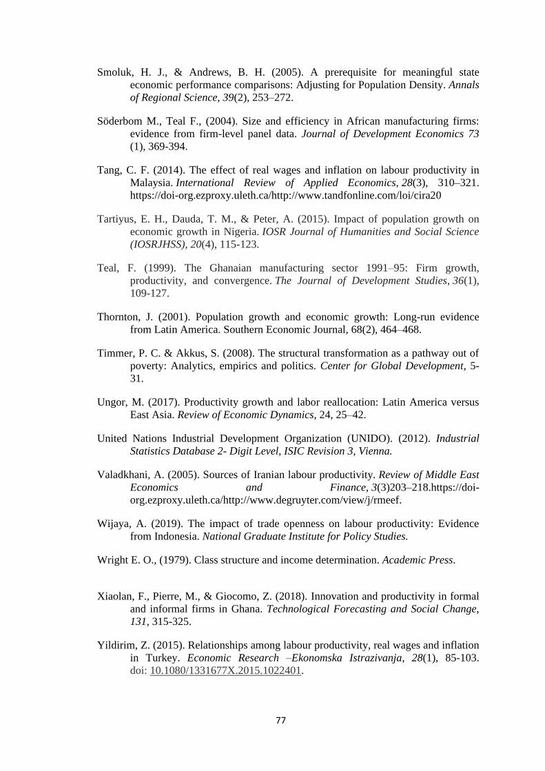
77
Smoluk, H. J., & Andrews, B. H. (2005). A prerequisite for meaningful state
economic performance comparisons: Adjusting for Population Density. Annals
of Regional Science, 39(2), 253–272.
Söderbom M., Teal F., (2004). Size and efficiency in African manufacturing firms:
evidence from firm-level panel data. Journal of Development Economics 73
(1), 369-394.
Tang, C. F. (2014). The effect of real wages and inflation on labour productivity in
Malaysia. International Review of Applied Economics, 28(3), 310–321.
https://doi-org.ezproxy.uleth.ca/http://www.tandfonline.com/loi/cira20
Tartiyus, E. H., Dauda, T. M., & Peter, A. (2015). Impact of population growth on
economic growth in Nigeria. IOSR Journal of Humanities and Social Science
(IOSRJHSS), 20(4), 115-123.
Teal, F. (1999). The Ghanaian manufacturing sector 1991–95: Firm growth,
productivity, and convergence. The Journal of Development Studies, 36(1),
109-127.
Thornton, J. (2001). Population growth and economic growth: Long-run evidence
from Latin America. Southern Economic Journal, 68(2), 464–468.
Timmer, P. C. & Akkus, S. (2008). The structural transformation as a pathway out of
poverty: Analytics, empirics and politics. Center for Global Development, 5-
31.
Ungor, M. (2017). Productivity growth and labor reallocation: Latin America versus
East Asia. Review of Economic Dynamics, 24, 25–42.
United Nations Industrial Development Organization (UNIDO). (2012). Industrial
Statistics Database 2- Digit Level, ISIC Revision 3, Vienna.
Valadkhani, A. (2005). Sources of Iranian labour productivity. Review of Middle East
Economics and Finance, 3(3)203–218.https://doi-
org.ezproxy.uleth.ca/http://www.degruyter.com/view/j/rmeef.
Wijaya, A. (2019). The impact of trade openness on labour productivity: Evidence
from Indonesia. National Graduate Institute for Policy Studies.
Wright E. O., (1979). Class structure and income determination. Academic Press.
Xiaolan, F., Pierre, M., & Giocomo, Z. (2018). Innovation and productivity in formal
and informal firms in Ghana. Technological Forecasting and Social Change,
131, 315-325.
Yildirim, Z. (2015). Relationships among labour productivity, real wages and inflation
in Turkey. Economic Research –Ekonomska Istrazivanja, 28(1), 85-103.
doi: 10.1080/1331677X.2015.1022401.
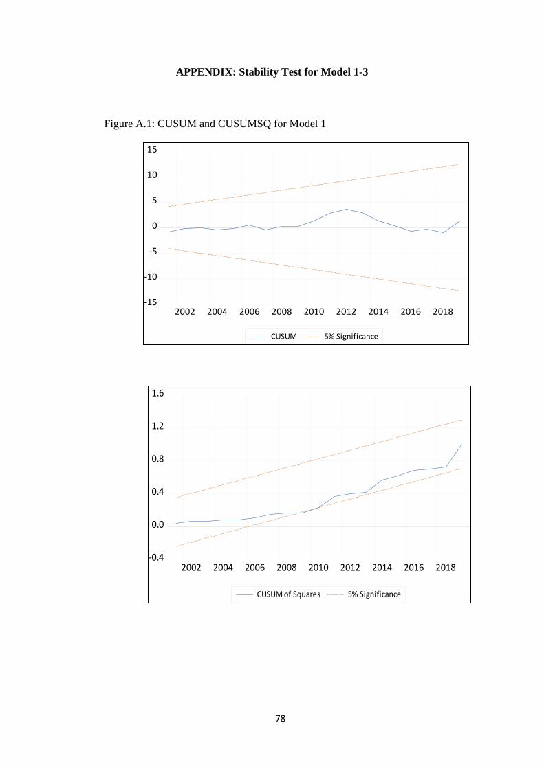
78
-15
-10
-5
0
5
10
15
2002 2004 2006 2008 2010 2012 2014 2016 2018
CUSUM 5% Significance
APPENDIX: Stability Test for Model 1-3
Figure A.1: CUSUM and CUSUMSQ for Model 1
-0.4
0.0
0.4
0.8
1.2
1.6
2002 2004 2006 2008 2010 2012 2014 2016 2018
CUSUM of Squares 5% Significance
79
Figure A.2: CUSUM and CUSUMSQ Test for Model 2
-15
-10
-5
0
5
10
15
98 00 02 04 06 08 10 12 14 16 18
CUSUM 5% Significance
-0.4
-0.2
0.0
0.2
0.4
0.6
0.8
1.0
1.2
1.4
94 96 98 00 02 04 06 08 10 12 14 16 18
CUSUM of Squares 5% Significance

80
Figure A.3: CUSUM and CUSUMSQ test for Model 3
-15
-10
-5
0
5
10
15
98 00 02 04 06 08 10 12 14 16 18
CUSUM 5% Significance
-0.4
-0.2
0.0
0.2
0.4
0.6
0.8
1.0
1.2
1.4
98 00 02 04 06 08 10 12 14 16 18
CUSUM of Squares 5% Significance