Population genomics of rapid evolution in natural

RESEARCH ARTICLE Open Access

Population genomics of rapid evolution innatural populations: polygenic selection inresponse to power station thermal effluentsDavid I. Dayan* , Xiao Du†, Tara Z. Baris†, Dominique N. Wagner†, Douglas L. Crawford and Marjorie F. Oleksiak

Abstract

Background: Examples of rapid evolution are common in nature but difficult to account for with the standardpopulation genetic model of adaptation. Instead, selection from the standing genetic variation permits rapidadaptation via soft sweeps or polygenic adaptation. Empirical evidence of this process in nature is currently limitedbut accumulating.

Results: We provide genome-wide analyses of rapid evolution in Fundulus heteroclitus populations subjectedto recently elevated temperatures due to coastal power station thermal effluents using 5449 SNPs across twoeffluent-affected and four reference populations. Bayesian and multivariate analyses of population genomicstructure reveal a substantial portion of genetic variation that is most parsimoniously explained by selection at thesite of thermal effluents. An FST outlier approach in conjunction with additional conservative requirements identifysignificant allele frequency differentiation that exceeds neutral expectations among exposed and closely relatedreference populations. Genomic variation patterns near these candidate loci reveal that individuals living near thermaleffluents have rapidly evolved from the standing genetic variation through small allele frequency changes at many lociin a pattern consistent with polygenic selection on the standing genetic variation.

Conclusions: While the ultimate trajectory of selection in these populations is unknown and we survey only a minorityof genomic loci, our findings suggest that polygenic models of adaptation may play important roles in large, naturalpopulations experiencing recent selection due to environmental changes that cause broad physiological impacts.

Keywords: Population genomics - empirical, Selective sweeps, Polygenic adaptation, Adaptation, Fish

BackgroundUnderstanding the population genetic basis of localadaptation is one of the principal goals of evolutionarybiology. Historically, theoretical models of adaptationhave focused on selection on one or a few genetic lociand populations that are mutationally limited. Underthese assumptions, a typical adaptive walk is a longprocess characterized by successive fixations of largeeffect alleles that arise via mutation after the onset ofselection [1]. Fixation of each adaptive allele leads to astrong selective signature among genomic variants inlinkage disequilibrium with the causative mutation,

producing a “hard sweep” [2]. This model has provided adetailed set of predictions that form the basis of manyempirical tests for selection [3, 4] and has been sup-ported by population genetic examinations of candidategenes, where the genotype to phenotype map for knownadaptive traits is well characterized [5, 6].While this standard hard sweep model is often invoked

to explain the genetic basis of adaptation among speciesthat diverged millions of generations ago or populationsthat diverged thousands of generations ago, many of themost salient evolutionary questions today, and perhapshistorically, occur on much more rapid time scales, e.g.adaptation to novel environments during species intro-ductions [7] and in spatially restricted populationscoping with global climate change [8]. Examples of rapidphenotypic evolution abound in both the laboratory andin nature and can occur over time scales as short as tens

* Correspondence: [email protected]†Xiao Du, Tara Z. Baris and Dominique N. Wagner contributed equally to thiswork.Rosenstiel School of Marine and Atmospheric Science, University of Miami,4600 Rickenbacker Causeway, Miami, FL 33149, USA

© The Author(s). 2019 Open Access This article is distributed under the terms of the Creative Commons Attribution 4.0International License (http://creativecommons.org/licenses/by/4.0/), which permits unrestricted use, distribution, andreproduction in any medium, provided you give appropriate credit to the original author(s) and the source, provide a link tothe Creative Commons license, and indicate if changes were made. The Creative Commons Public Domain Dedication waiver(http://creativecommons.org/publicdomain/zero/1.0/) applies to the data made available in this article, unless otherwise stated.

Dayan et al. BMC Evolutionary Biology (2019) 19:61 https://doi.org/10.1186/s12862-019-1392-5

http://crossmark.crossref.org/dialog/?doi=10.1186/s12862-019-1392-5&domain=pdf

http://orcid.org/0000-0001-5001-4062

mailto:[email protected]

http://creativecommons.org/licenses/by/4.0/

http://creativecommons.org/publicdomain/zero/1.0/

of generations [9]. Hard sweeps are unlikely to drivethese rapid phenotypic shifts because there is insufficienttime to overcome the lag period in the standard model;in this standard model, adaptation requires an adaptivemutation to appear and reach high enough frequency toescape stochastic loss. Instead of proceeding via hardsweeps, rapid evolution is proposed to proceed by eithersoft-sweeps or polygenic adaptation. Under the softsweep model, selection sweeps adaptive alleles to highfrequency, but these alleles are borne on multiplehaplotypes, either because they arise independently orthey are present in the standing genetic variation longenough to become unlinked from nearby variation [10, 11].In the latter case, soft sweeps can facilitate rapid evolutionbecause selection can act on alleles already segregating atmoderate frequency at the onset of selection [12], avoidingthe aforementioned lag period.Soft sweeps appear to have driven local adaptation in a

number of empirical examinations [13–16]. Yet, thetraits under selection in such studies often demonstratea simple, oligogenic genetic architecture. In contrast,natural selection is expected to operate primarily onhighly integrated, complex performance traits [17] thatare characterized by highly polygenic genetic architec-tures [18], i.e. quantitative traits. In the case of quantita-tive traits, genetic architecture may be so diffuse as toapproximate Fisher’s infinitesimal model, which assumesan infinite number of loci each with an infinitely smalleffect [19], and polygenic adaptation may play an import-ant role [20]. Multilocus simulations suggest that althoughsweeps at a minority of loci are possible, polygenic geneticarchitectures reduce the number of adaptive fixations thatcontribute to adaptation and that phenotypic evolutioncan proceed extremely rapidly via minor changes in allelefrequency changes at many loci [21–23].In the case of local adaptation, these predictions

regarding the nature of adaptive genetic variants areadditionally complicated by the influence of gene flow[24]. Gene flow can swamp locally advantageous alleles,leading to a bias towards large effect alleles that aremore resistant to swamping [24], or tight linkage amongmultiple small effect loci that segregate in the popula-tions as de facto large effect alleles [25]. This influenceof gene flow leads to a tendency against small allelefrequency changes at many loci and towards sweep sce-narios, where adaptive allele frequencies vary greatlyacross populations [26]. Despite this predicted tendencyfor gene flow to bias the evolution of quantitative traitstowards sweeps of large effect alleles, polygenic adapta-tion may play a significant role in the short run, becauseit takes time for “supergene” structural variants orsimilar effects to establish, e.g. [27, 28], or variants inlow recombination areas of the genome that protectgenomic regions containing adaptive variants from gene

flow, e.g. [29], to enter the population and increase infrequency [30].In this investigation, we seek to test these predictions

regarding the nature of genetic variants contributing torapid local adaptation in populations of the estuarinefish Fundulus heteroclitus exposed to the thermal efflu-ents of coastal power stations. We sampled F. heterocli-tus populations near the effluents of two power stations:Oyster Creek nuclear generating station in New Jerseyand Brayton Point generating station in Massachusetts.Thermal effluents produced by coastal power stationsprovide a recent source of environmental variation thatis both localized and well quantified. Effluents from bothpower plants have produced significant thermal impactssince the beginning of their operation in the late 1960s.The Oyster Creek thermal effluent is discharged along amodified river for approximately 3 km into the intra-coastal Barnegat Bay. Temperatures range from 10 to13 °C above ambient at the discharge site and 4–5 °Cabove ambient where Oyster Creek joins Barnegat Bay.Beyond this point, the effluent’s thermal influence is lim-ited to a ~ 2 km radius from the mouth of Oyster Creek[31]. Documented ecological impacts of thermal input atOyster Creek include maintenance of non-native,warm-adapted species not found elsewhere in the region[32] as well as decreased growth rates and failed spawn-ing events in benthic molluscs [31]. At Brayton Point,effluent is released into the surrounding estuary, MountHope Bay, at 7–16 °C above ambient temperatures. Thiseffluent leads to ~ 1 °C temperature anomaly throughoutMount Hope Bay [33], but has varied thermal impactson smaller spatial scales due to incomplete mixing andadvection of the thermal plume [34]. There are fewpredicted ecological impacts of the thermal effluent atBrayton Point [35, 36], although increased temperaturemay interact with other anthropogenic stressors in thisregion [37].Power station thermal effects lead to thermal adapta-

tion among exposed populations. Indeed, comparisonsof natural populations living in or near thermal effluentshave traditionally been used to parse adaptive geneticvariation from neutral genetic variation. Allelic selectionamong electrophoretic variants of candidate loci isfrequently reported in populations exposed to thermaleffluents [38–40]. In F. heteroclitus, a northern thermaleffluent population has allele frequencies more similarto distant, warm-adapted southern populations thanmore closely-related northern populations at severalallozyme loci [41]. Selection due to thermal effluents canalso elicit rapid phenotypic evolution. Largemouth bass(Micropterus salmoides) living in effluent ponds demon-strate increased frequency of more thermally stableisozymes after fifteen generations, and allele frequenciesat these loci return to ancestral levels after just ten [42].

Dayan et al. BMC Evolutionary Biology (2019) 19:61 Page 2 of 20

While the genetic architecture of thermal adaptation isnot well known [43], we expect thermal adaptation tohave a highly polygenic basis, in contrast with otherrecent population genomic studies of rapid evolution,such as rapid evolution of resistance to pesticides. Selec-tion in response to a single or related chemicals is oftenmediated through a single pathway or even a singlegenetic locus [44–46], and this specificity lends itself toa narrow genomic basis of adaptation [47]. Temperaturebroadly impacts all physiological systems through itseffects on biochemical reaction rates and biomolecularstructures [48, 49]. Additionally, thermal variation hasindirect impacts mediated through more complexecological changes, e.g. species interactions [50], furtherincreasing the number of genetic variants that mightcontribute to fitness in an altered thermal environment.Accordingly, rapid thermal adaptation is likely to have adifferent genomic basis than other well-understoodexamples of rapid evolution because the selection targetis expected to be so broad.Our investigation extends early allozyme data by

directly examining variation at thousands of genotyping-by-sequencing derived genetic markers. We providepopulation genomic, functional genomic and phenotypicevidence suggestive of adaptation in natural Fundulusheteroclitus populations exposed to thermal effluents.We then consider the genomic variation near candidateadaptive loci in light of recent theory regarding thenature of genetic variants contributing to local adapta-tion. Specifically, our data sheds light on the nature ofadaptive variants when (i) selection is very recent, (ii)the selective environment is spatially restricted withrespect to the extent of historical gene flow among pop-ulations, (iii) the effective population size is large, and(iv) the traits under selection are likely to have a highlypolygenic basis. Under these restrictions we do notexpect hard sweeps to play a significant role, and theorysuggests that adaptation might occur via soft sweeps orpolygenic adaptation.

ResultsSamples and filteringAfter filtering on the basis of depth, missingness, minorallele frequency and Hardy-Weinberg equilibrium ourfinal single nucleotide polymorphism (SNP) datasetconsisted of 5449 SNPs among 239 individuals from sixpopulations. F. heteroclitus populations were sampled intwo “triads” [51], each consisting of a single thermaleffluent (TE) site bordered on either side along the coastby a reference site (Fig. 1). The two TE populations areOyster Creek and Brayton Point (Table 1). Mean readdepth per SNP per individual was 26.29 ± 0.43 for thefull SNP dataset (Additional file 1: Figure S1).

a

b

Fig. 1 Sampling locations and triad design. Each thermal effluentpopulation (red markers) is surrounded by two referencepopulations (blue markers). The northern triad (a) is the BraytonPoint generating station population and its references. The southerntriad (b) consists of the Oyster Creek nuclear generating stationpopulation and its references. Map data are drawn from USDepartment of Census and visualized using the maps package in R

Table 1 Pairwise estimates of nucleotide diversity andpopulation differentiation among experimental populations

N RB OC Mg SR BP HB

RB 40 0.1518 0.0095 0.0081 0.1089 0.1256 0.1107

OC 36 0.1198 0.0973 0.0104 0.107 0.1261 0.1095

Mg 37 0.1483 0.1184 0.1479 0.0891 0.1063 0.0908

SR 41 0.1402 0.1111 0.1353 0.1055 0.0252 0.0318

BP 47 0.1418 0.1125 0.1367 0.1048 0.1026 0.0272

HB 38 0.138 0.1093 0.1331 0.1048 0.1028 0.1015

Values above the diagonal are mean pairwise FST values across all 5.4 k SNPs.Values along the diagonal (bold) are mean nucleotide diversity (π) withinpopulations. Values below the diagonal are mean proportion of pairwisedifferences (π). Population abbreviations: Oyster Creek Triad (SouthernReference – Rutgers Basin (RB), TE Population – Oyster Creek GeneratingStation (OC), Northern Reference – Mantoloking, New Jersey (Mg)) BraytonPoint Triad (Southern Reference – Succotash Marsh, Matunuck, Rhode Island(SR), TE Population – Brayton Point Generating Station (BP), NorthernReference – Horseneck Beach, Massachusetts (HB)). N: number of individuals infinal SNP dataset


Genome-wide diversity estimates and neutral populationgenetic structureWe identified substantial genetic diversity both withinand among populations (Tables 1 and 2). Mean esti-mated pairwise FST values using the full SNP datasetranged from 0.008–0.126 across the populations. Meangenetic diversity (π) estimates ranged from 0.103–0.148among populations and 0.097–0.152 within each popula-tion (Table 1). Note, however, that these π estimates areinflated relative to true genome-wide averages becausethey are calculated using only SNPs from polymorphicsequence tags used to generate our SNP dataset, insteadthese data should be used to compare among popula-tions in this study.Analysis of molecular variance (AMOVA) on the full

SNP dataset partitioned 9.6% of the total genotypicvariation to differences among triads, 0.7% among popu-lations within a triad and the remainder (89.7%) withineach population. The variance component among triadsin the AMOVA was not significant while the othervariance components were significant, suggesting thatalthough the portion of genetic variation among triads islarge, much of this variation is attributable to amongpopulations structure; i.e., the larger grouping (triads) isan artificial product of the hierarchical population sam-pling we employed. AMOVA conducted on a “neutral”SNP dataset that excluded outliers from any pairwisecomparison within a triad produced qualitatively similarresults, with the exception that the extent of amongtriad variation was reduced (Additional file 2: Table S1).We examined populations within each triad for isola-

tion by distance (IBD) using Mantel Tests (Fig. 2) [52].While there is significant IBD across all populationsamong triads (p < 0.01, Mantel test of pairwise FST basedon all loci vs. pairwise geographic distance, 9999 simula-tions), neither triad showed significant IBD among itspopulations (Mantel test, p > 0.5, 9999 simulations), noris there a trend towards IBD using genome wide FST(Fig. 2). Therefore, the demographic assumptions inher-ent to outlier analyses are strongly violated whencomparisons drawn across triads but valid within triads.STRUCTURE identified no genetic substructure

within a triad when all 5449 SNPs were used, i.e. best kwas 1. Similarly, no structure was observed when using

a putatively neutral set of SNPs created by excludingoutliers. STRUCTURE detected population structurewithin the Brayton Point triad after thinning the fulldataset for SNPs in linkage disquilibrium (r2 > 0.5)(Additional file 3: Figure S8). The best K was 3, witheach population dominated by a single ancestry cluster(Additional file 4: Figure S3). No similar sensitivity tolinked SNPs was found in the Oyster Creek triad. Best kwas 1 and there was no large difference in cluster mem-bership among the three populations (Additional file 4:Figure S3).

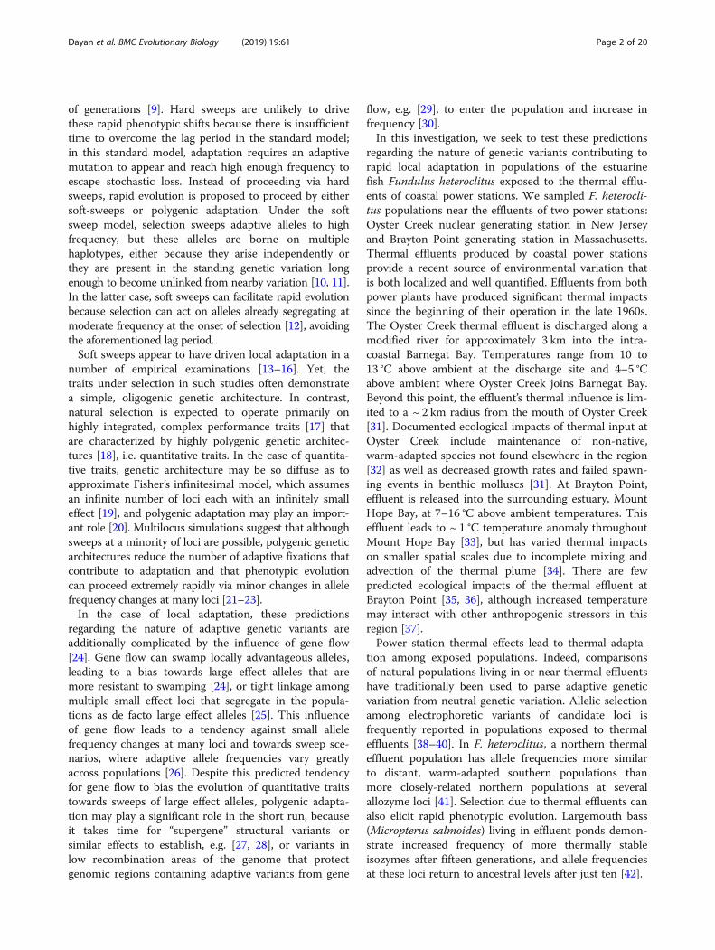
Outlier analyses and candidate lociTo distinguish loci that have neutral divergence patternsfrom loci that may be evolving by natural selectionamong populations within a triad, we conducted outlieranalyses using the FDIST2 algorithm implemented inLositan [53]. An outlier analysis uses empirical data tosimulate a neutral distribution of FST values for a givenlevel of expected heterozygosity. SNPs with FST valuesthat significantly exceed the simulated distribution witha modified FDR of 5% [54, 55] were considered outliers.The numbers of significant outliers in any single pairwisecomparison among populations ranged from 3.2 to 5.7%of the total SNPs (Fig. 3) and were distributed across theobserved heterozygosity range (Additional file 5: FigureS2). Within the Oyster Creek triad, 624 SNPs wereidentified as outlier loci in any of the three pairwisecomparisons; 619 were identified in the Brayton Pointtriad (Fig. 3).We identified potentially adaptive SNPs among these

outliers using the triad experimental design. Specifically,we refer to SNPs that were identified as outliers in bothpairwise comparisons of TE vs. reference populations,but not in the reference vs. reference comparison ascandidate loci (see Fig. 3) [51] – see Discussion for de-tails about this evolutionary inference. This approachrevealed 94 candidate loci in the Oyster Creek TE popu-lation and 36 candidate loci in the Brayton Point TEpopulation where population differentiation may be dueto selection unique to the effluent site. The candidateloci for each triad are significantly enriched for SNPswith reduced nucleotide diversity (θπ) and Tajima’s D(Table 3).

Inferring selection from population genetic structureGenetic structure potentially resulting from varyingselection among populations within a triad was inferredusing two methods: a model-based Bayesian approach(STRUCTURE) using the most differentiated loci and anon-model-based multivariate approach (discriminantanalysis of principal components (DAPC)) using the fullSNP dataset (Fig. 4, Additional file 4: Figure S3). Given anumber of ancestral populations or genetic clusters (k),

Table 2 AMOVA Results

Variance Component df % variation Φ Statistic P

Among triads 1 9.59 ΦCT = 0.09593 p = 0.099

Among populationswithin triads

4 0.69 ΦSC = 0.00762* p < 0.00001

Among individualswithin populations

472 89.72 ΦST = 0.10282* p < 0.00001

Total 477


STRUCTURE estimates the probability that an individualderives its ancestry from a particular genetic cluster at theloci provided. DAPC maximizes among populationdifferences while minimizing within group variation bycombining principal components of genetic variation.

StructureFirst, we ran STRUCTURE using only SNPs that demon-strated significant differentiation among populations.This STRUCTURE analysis used the union of outlierSNPs from all three pairwise comparisons within a triad(624 SNPs for the Oyster Creek triad and 619 for theBrayton Point triad) at a range of putative populationclusters between 1 and 6. Thus these results do notreflect population genetic structure genome-wide (seeabove for these results); rather they reflect differencesamong the populations at the most differentiated loci.These STRUCTURE analyses produced different resultsbetween the two triads. For the Oyster Creek triad, K = 2captured most of the structure among the populations atthe most differentiated loci (Fig. 4a, see methods fordetails). Using two population clusters, the two referencepopulations group with one another, separate from theTE population. While there are admixed individuals inall populations, the two reference populations weredominated by a single cluster while the TE populationwas dominated by a second cluster. Group membershipin the first cluster was 75 and 68% for the two referencepopulations and 5% for Oyster Creek (TE). Results atincreasing K values are qualitatively similar; the identityof a population as reference or effluent-affected predictsthe major inferred ancestry cluster among the OysterCreek triad populations. For the Brayton Point triad, K= 3 explains most of the structure among populations

(Fig. 4b, see methods for details). At K = 3, each popula-tion is dominated by its own cluster, such that eachpopulation is unique. These results are robust tolinkage disequilibrium (LD) among differentiatedSNPs. Submitting an LD-thinned set of outlier SNPsto STRUCTURE produces qualitatively similar results(Additional file 6: Figure S9).For both the Oyster Creek and Brayton Point triads

we conducted an additional analysis. The most differen-tiated loci among populations within a triad are notrepresentative of the genome-wide site frequencyspectrum. Pairwise outliers are enriched for among lociwith lower minor allele frequency (one tailed Wilcoxonrank sum test p = 0.038, and p = 2.2 × 10− 16, for BP andOC respectively). To investigate the possibility that thepopulation genetic structure described above varies fromstructure at loci in the neutral SNP dataset because ofdifferences in site frequency spectrum rather than highdifferentiation, e.g. STRUCTURE is more sensitive whenusing more or less common alleles, we bootstrapsampled the neutral dataset to match the outlier datasetanalyzed above with respect to minor allele frequency.This site frequency spectrum matched neutral datasetdid not demonstrate any evidence of structure within atriad suggesting that the structure identified usingdifferentiated loci is not an artifact arising from the useof STRUCTURE on datasets that varied in their sitefrequency spectra.

Discriminant analysis of principal componentsWe also conducted discriminant analysis of principalcomponents (DAPC) for the triads [56]. In contrast tothe STRUCTURE results, DAPC performed on the fullSNP dataset identified similar patterns of population

0.025

0.050

0.075

0.100

0.125

Geographic Distance (km)

FS

T

Between

BP

OC

100 200 300

Fig. 2 Isolation by distance. Geographic distance along the coast vs. genetic distance as estimated by mean genome-wide FST value forcomparisons within the Brayton Point (BP, filled circles) and Oyster Creek (OC, filled triangles) triads and comparisons between triads (opendiamonds). There is significant isolation by distance for all comparisons (p < 0.01, Mantel test, 9999 simulations), but not within triads (p > 0.5,Mantel test, 9999 simulations)


structure for both triads. The first discriminant functionin DAPC represents the major axis of genetic structureamong populations. The three populations were distrib-uted along this primary axis of genetic variation in apattern consistent spatial autocorrelation; the TE popu-lation is intermediate to the two references (Fig. 4d).The second major axis of genetic variation used todiscriminate between the populations explained lessvariation (eigenvalues Brayton Point: 297.8 vs. 169.6;

eigenvalues Oyster Creek: 84.4 vs. 51.2) and revealed apopulation genetic structure pattern that is not con-sistent with their geographic distribution. Along thesecond major axis of genetic variation the two refer-ence populations demonstrated substantial overlapwhile the TE population is distinct. Thus, for bothtriads the second major axis of genetic differencesamong populations for all 5449 loci in the SNP data-set does not fit the neutral expectation: the two refer-ence populations are more similar to each other thaneither is to the TE population.

Environmental association - redundancy analysisFinally, we used two multivariate approaches, redun-dancy analysis (RDA) and partial redundancy analysis(pRDA) [57] to examine the extent to which spatialvariables and the presence of effluents could be used toexplain patterns in the genetic variation among popula-tions (Table 4). For Oyster Creek, the first 51 principalcomponents of account for 53% of the total geneticvariation. Only the first distance based Moran’s eigen-vector map (dbMEM) had significant Moran’s I. TheRDA was significant (p = 0.001, 1000 permutations).Variance partitioning revealed that 0.51% of the totalgenetic variation was attributable to spatial variationalone (27.9% of FST), 0.49% attributable to effluents(26.8% of FST) and no variation explained jointly(Table 4). The total constrained variance accountedfor 54.6% of FST. pRDA demonstrated that effluentsand spatial distance each significantly explainedgenetic variation once controlling for the other (p =0.001, 1000 permutations) (Table 4).For Brayton Point the first 55 principal components of

account for 44% of the total genetic variation. Only thefirst dbMEM had significant Moran’s I. The RDA wassignificant (p = 0.001, 1000 permutations) with 0.86% ofthe genetic variation attributable to spatial variation alone(13.5% of FST), 0.89% attributable to effluents (13.9% ofFST) and no variation explained jointly (Table 4). The totalconstrained variance accounted for 27.3% of FST. pRDAdemonstrated that effluents and spatial distance eachsignificantly explained genetic variation once controllingfor the other (p = 0.001, 1000 permutations) (Table 4).

Oys

terC

reek

vs. N

orth

ern

Reference Oyster Creek vs. Southern

Reference

Reference vs. Reference

15294

‘candidate SNPs’ 162

1

66 36

115

a

Bra

yton

Poi

ntvs

. Nor

ther

n

Reference Brayton Point vs. Southern

Reference

Reference vs. Reference

25536

‘candidate SNPs’ 94

1

91 43

102

b

Fig. 3 Candidates. Number of significant outliers in pairwisecomparisons of thermal effluent (TE) populations vs. referencepopulations (red circles) and pairwise comparisons of reference vs.reference populations (blue circles) for (a) the Brayton Point (BP) and(b) the Oyster Creek (OC) (b) triads. Candidate loci for each triad(‘candidate’) are those that are significant outliers in both TE vs.reference comparisons (red circles), but not in the reference vs.reference comparison (blue)

Table 3 Nucleotide Diversity and Allele Frequency Spectrum atCandidate Loci vs. Genome-wide

Triad SNP set θπ Tajima’s D

Brayton Point Candidate LociAll Loci

0.0524***0.0873

−0.831****− 0.599

Oyster Creek Candidate LociAll Loci

0.0693****0.1262

−0.769****− 0.431

Median values of within triad pairwise nucleotide divergence (θπ), and Tajima’sD for the triad candidate SNPs vs all SNPs. Asterisks denote significance levelof one-tailed Wilcoxon rank sum test (*: p < 0.05, **: p < 0.01, ***: p < 0.001,****: p < 0.0001)


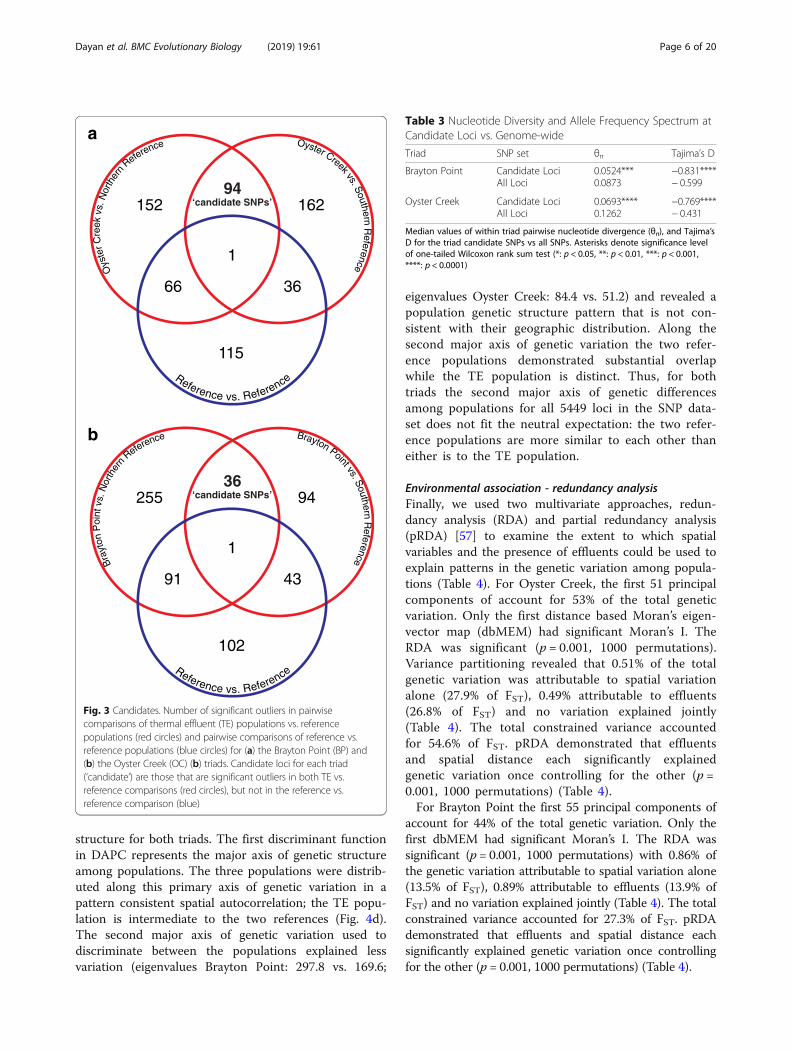
Putatively adaptive allele frequency changes are smallWe examined the distribution of all allele frequency dif-ferences between reference and TE populations (Fig. 5aand b). Major allele frequencies are similar for both TEand reference populations (Fig. 5). There were no fixeddifferences between populations. In fact, all alleles at

fixation in any one population were the major alleleoverall, both within and among the two triads. For eachTE population and its two references, change in allelefrequencies for all SNPs have a maximum of 33% changefor Oyster Creek and a maximum of 45% for BraytonPoint. At the majority of loci (90%), allele frequency

a

b

c

d

Fig. 4 Population genetic structure within triads. STRUCTURE plots for Oyster Creek (a) and Brayton Point (b) triads based on data from the mostdifferentiated loci (all pairwise outliers within a triad). Each individual is represented with a radial line that is partitioned into colors according tomodeled admixture proportions for k ancestral populations. Results for k = 2–4 are presented with best k denoted by an asterisk. DAPC plots forOyster Creek (c) and Brayton Point (d) triads using the full SNP dataset. Each individual’s position along the first two principal components(discriminant functions) is shown with a point, with populations identified by color. The relative eigenvalues of the first (horizontal) and second(vertical) principal components are shown in the bar plot at the bottom right of each figure

Table 4 RDA results for both triads considered jointly and each triad separately

Dataset Percent Total Constrained Variance FST Explained Explanatory Variables PVE FST Explained per variable

Both Triads 0.77% 6.5% dbMEM-1*** 0.40% 3.4%

Effluents*** 0.36% 3.1%

Oyster Creek 0.99% 54.6% dbMEM-1*** 0.51% 27.9%

Effluents*** 0.49% 26.8%

Brayton Point 1.73% 27.3% dbMEM-1*** 0.86% 13.5%

Effluents*** 0.89% 13.9%

Asterisks denote significance of the variable in pRDA after conditioning the genetic data on all other variables, PTCV is percent total constrained variance amongthe major principal components of genetic variation for the full model, FST explained is the portion of among population genetic differentiation (FST) explained bythe total constrained variance weighted by the variance retained in the major principal components of genetic variation, PVE is percent of variance that isexplained by each of the explanatory variable according to variance partitioning. Significant explanatory variables are indicated with the followingsymbols: ***P = 0.001


differences are less than 10% between the Oyster CreekTE population and the mean of both Oyster Creek refer-ence populations. Similarly, 92% of loci have less than10% allele frequency differences for the same compari-son in the Brayton Point triad.For the candidate loci, the allele frequencies changes

are also small. Among candidate loci, the maximumallele frequency change is 8% between the TE populationand both reference populations for both the OysterCreek and the Brayton Point triads (Fig. 5c and d). Puta-tively adaptive alleles (those favored in the effluentpopulation) are rarely private alleles globally becausemost are the major allele overall, or the adaptive minorallele in the TE population is observed as the minorallele in the other triad.

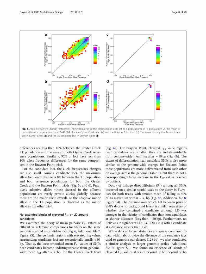
No extended blocks of elevated FST or LD aroundcandidatesWe examined the decay of mean pairwise FST values ofeffluent vs. reference comparisons for SNPs on the samegenomic scaffold as candidate loci (Fig. 6, Additional file 7:Figure S5). The genomic regions with elevated FST valuessurrounding candidate loci are exceptionally small: < 30bp. That is, the loess smoothed mean FST values of SNPsnear candidates become indistinguishable from genome-wide mean FST after ~ 30 bp, for the Oyster Creek triad

(Fig. 6a). For Brayton Point, elevated FST value regionsnear candidates are smaller; they are indistinguishablefrom genome-wide mean FST after ~ 18 bp (Fig. 6b). Theextent of differentiation near candidate SNPs is also moresimilar to the genome-wide average for Brayton Point;these populations are more differentiated from each otheron average across the genome (Table 1), but there is not acorrespondingly large increase in the FST values reachedby outliers.Decay of linkage disequilibrium (R2) among all SNPs

occurred on a similar spatial scale to the decay in FSTva-lues for both triads, with smooth mean R2 falling to 50%of its maximum within ~ 30 bp (Fig. 6c, Additional file 8:Figure S4). The distance over which LD between pairs ofSNPs decays to background levels is similar regardless ofwhether they contained a candidate, although LD wasstronger in the vicinity of candidates than non-candidatesat shorter distances (less than ~ 50 bp). Furthermore, noSNP was in significant LD (BY-FDR < 0.1) with a candidateat a distance greater than 1 kb.While data at longer distances are sparse compared to

data within about twice the distance of the sequence tagsused to generate our dataset (128 bp), we also conducteda similar analysis at larger genomic scales (Additionalfile 7: Figure S5). We found no evidence of islands ofelevated FST values at scales beyond 50 bp. Beyond 50 bp

a

b

c

d

Fig. 5 Allele Frequency Change Histograms. Allele frequency of the global major allele (of all 6 populations) in TE populations vs. the mean ofboth reference populations for all 5449 SNPs for the Oyster Creek triad (a) and the Brayton Point triad (b). The same for only the 94 candidateloci in Oyster Creek (c) and the 36 candidate loci in Brayton Point (d)


and up to 1 megabase from candidate loci, the 95% con-fidence interval of the smoothed mean FST value remainsbelow the genome-wide mean level of differentiationbetween each of the two pairs of effluent vs. referencecomparisons within the triad.

Annotation term enrichmentWe conducted a enrichment analysis of annotation termsto assess whether loci identified as candidates may haveroles in biological pathways or processes that are canonic-ally involved in thermal adaptation (Additional file 9:Table S2). Approximately half of sequence tags with adap-tive SNPs mapped with genes in the DAVID database: 42of 94 candidates for Oyster Creek map to the databaseand 21 of 36 for Brayton Point. One cluster of similarfunctional annotation terms was significantly enriched(EASE score > 1.3) in each triad: GTPase regulator activityin Brayton Point and protein complex assembly in OysterCreek. However, several gene annotation clusters areenriched at lower EASE scores (0.5–1.2) and are salientbecause of their association with thermal adaptation.Functional annotation clusters for synaptic transmissionand neuronal morphogenesis are enriched in both triads.

Critical thermal maximumTo assess whether exposure to thermal effluents has ledto an increase in thermal tolerance, we measured criticalthermal maxima (CTmax) in F. heteroclitus collectedfrom Oyster Creek and its northern reference populationafter acclimation to laboratory conditions. Oyster Creekindividuals demonstrated a significant, but minor in-crease in thermal tolerance relative to the northernreference population (ANOVA, p = 0.0483, N = 98). Thecritical thermal maximum for Oyster Creek was 39.7 ±0.07 °C (mean ± s.e.) while the critical thermal maximumfor the northern reference was 39.5 ± 0.07. °C. Thesedifferences correspond to a PST (phenotypic divergencein a trait across populations) value of 0.67, which ex-ceeds FST among these populations (FST = 0.01), suggest-ing that selection may drive this difference in thermaltolerance. However, divergence in genetic architectureand narrow-sense heritability for this trait may alsodrive the observed divergence. To examine the ro-bustness of the PST-FST comparison to these effects,we bootstrapped sampled the data according to [58].This analysis suggests divergence in the trait valuesexceeds expected divergence under genetic drift giventhe extent of genetic differentiation among thesepopulations (Additional file 10: Figure S7).

DiscussionMuch of our theoretical understanding of adaptiveevolution assumes a new mutation that rises to fixationquickly after the onset of selection [1]. Yet, much of

Mea

n F

ST

Mea

n F

ST

a

b

0.00

0.25

0.50

0.75

1.00

0 50 100 150

Distance (bp)

0.000

0.025

0.050

0.075

0.100

0 25 50 75 100

Distance (bp)

0.00

0.04

0.08

0.12

0 25 50 75 100

Distance (bp)

r2

c

Fig. 6 Decay of FST and LD near candidate SNPs. a and b Meanreference vs. effluent FST values at SNPs physically near candidate SNPsfor the Oyster Creek triad (a) and Brayton Point triad (b). Distance ispresented in base pairs from candidate SNP, smoothing line (red) isthe Loess-smoothed mean FST value with 95% confidence intervals,dashed line is the mean genome-wide FST value estimate (dashedblack line) for both reference vs effluent comparisons within the triad,red SNPs are other candidate loci. c Decay of linkage disequilibrium(r2): R2 among single SNP pairs, with loess smoothing line for SNP pairsthat contain a candidate (red) and those that do not (black)


adaptive evolution may involve neither new alleles, norfixation of a single allele [20]. This latter scenario is par-ticularly likely in natural populations with large effectivepopulation sizes, when selection is recent and the selec-tion target is highly polygenic [10, 59]. Rapid evolutionof whole organism performance is particularly salient toconcerns regarding populations’ abilities to cope withrapidly changing environmental conditions. Tocharacterize the genomic signature of rapid adaptation,we analyze changes in allele frequencies associated withrecent thermal adaptation in two sets (triads) of popula-tions. First, we examine demographic relationshipsamong our sampled populations to understand the im-pacts of neutral processes on allele frequency differenceswithin a triad. Then we establish that allele frequenciesat a subset of the most differentiated loci within a triaddo not follow a pattern parsimoniously explained bydemographic processes, suggesting that selection uniqueto the thermal effluent environment may drive the dif-ferentiation at some loci. We then identify candidate lociusing our triad experimental design in conjunction withan outlier analysis and further assessed that these candi-date loci may be subject to selection through enrichmentanalysis of gene annotation terms and an examination ofnucleotide diversity. Finally, we describe the signature ofthis putative selection on linked genetic variation nearthe candidate loci.

Evidence of recent selection in response to thermaleffluentsPopulation genetic structureUsing STRUCTURE on both the full SNP dataset and aset of putatively neutral SNPs, we find no evidence ofstrong population genetic structure in either triad, meanFST within a triad is very low and there is no significantpattern of isolation-by-distance at this genome-wideview. Yet several lines of evidence reduce our confidencein this conclusion: the Mantel tests used to test for IBDwithin a triad have limited power owing to the small sizeof the matrices [60], STRUCTURE is relatively poor atrevealing structure at very low levels of differentiation[61], after removing correlated SNPs, STRUCTUREresolves each of teh Brayton Point triad populations intotheir own clusters, the AMOVA reveals significantamong population variation within triads and the RDAdemonstrates that spatial autocorrelation contributessignificantly to a small portion of genetic variationwithin a triad. Taken together, these results suggest thatfor most loci, historic gene flow among our samplinglocales should limit the extent of allele frequenciesvariation among populations within a triad. However, atthe most differentiated loci, we expect a different pat-tern. In our sampling design, each effluent-affectedpopulation is flanked by two reference populations. For

genomic regions subjected to only neutral or demo-graphic forces, the expectation is that the two referencepopulations will demonstrate greater allele frequencydifferences than between a reference population and theintermediately located TE population. Patterns of geneticvariation where the two more distantly located referencepopulations are more similar to each other than either isto the TE population are difficult to account for underneutral scenarios and may be due to selection unique tothe TE population [51]. While we attribute thesenon-neutral patterns of divergence between TE and bothreference populations to the temperature changes nearthe thermal effluents, other environmental or ecologicalfactors could also be important.We evaluate the neutral assumption of population

genetic structure using three approaches. First, we utilizea model-based Bayesian approach (STRUCTURE)applied to the loci identified as outliers in any one of thepairwise comparisons within a triad. Thus we use themost differentiated loci to reveal subtle population gen-etic structure at loci whose differentiation is potentiallyinfluenced by selection [62]. Such an approach isfrequently used to describe population structure whendifferentiation at most markers is low, but selectionmaintains differentiation at a subset a loci [63–65],despite violation of some model assumptions. To com-plement these results, we conduct two multivariate ana-lyses on the full SNP datatset: a discrimination analysis(DAPC) [56] that maximizes the weighting of allele fre-quencies among principal components of genetic vari-ation to describe differences among populations andredundancy analysis (RDA) to characterize differencesamong populations along orthogonal principal compo-nents of genetic variation and to examine the extent towhich spatial autocorrelation and/or the presence ofeffluents significantly contributes to patterns of geneticvariation among populations.For the Oyster Creek triad there are two genetic clus-

ters among outliers inferred by STRUCTURE. Individ-uals from the two reference populations primarily derivetheir ancestry at the most differentiated loci from onecluster, while the TE population is dominated by asecond cluster. This pattern is consistent across therange of ancestral genetic clusters that we model andleads us to reject the neutral hypothesis for genetic vari-ation among the most differentiated loci. The DAPCanalyses support this finding. The second axis in DAPCusing the full SNP dataset indicates a non-neutral pat-tern where the TE population is distinct from both refer-ence populations with little distinction between the tworeference populations. This divergence in the TE popula-tion in the second axis is different from the primary axisof genetic variation that follows a neutral pattern, wherethe position along the genetic axis of a population


correlates with its geographic distribution. These pat-terns among all SNPS are expected if selection is occur-ring at the effluent site; we expect a mosaic of historicevolutionary forces to drive the differences observedamong SNPs randomly sampled along the genome, witholder, neutral forces shaping the majority of variation,but recent selection unique to the effluent site drivingdifferentiation at some loci in the standing geneticvariation.In the Brayton Point triad, populations are more

strongly differentiated (FST values ~ 0.03) than theOyster Creek triad (FST values ~ 0.01), and STRUCTUREanalysis using the most differentiated loci suggests thateach population is unique. When we examine all loci forthe Brayton Point triad using DAPC, however, we find asimilar pattern as in the Oyster Creek triad. The majoraxis of genetic variation separates each of the popula-tions in a pattern consistent with its geographic position,but the two reference populations are more similar toeach other along the second major axis of geneticvariation than either is to the TE population. In both theOyster Creek triad and Brayton Point triad, the secondlargest component of genetic variation among the popu-lations occurs in a pattern that is not consistent withneutral evolution. Therefore, we interpret the DAPCresults as evidence of selection in both TE populationsbut caution that the STRUCTURE results do notcorroborate this interpretation for Brayton Point wherepopulation differentiation is stronger.To further examine the possibility that genetic vari-

ation within a triad is explained by both demographyand the presence of effluents, we conducted three sets ofpartial RDAs: a set of global RDAs using both triads anda set of RDAs within each triad. Permutation of thegenetic data in the RDA using data from both triadsdemonstrates that both spatial autocorrelation and efflu-ents significantly contribute to genetic variation at thisspatial scale. This result suggests that both effluentdriven selection and isolation by distance influence allelefrequencies to some extent. Yet, the model at the globalspatial scale appears to underfit the genetic data. Theportion of genetic data constrained by the model ismuch less than the variation among populationsrevealed by the AMOVA and average genome-wide di-vergence estimated by FST. One possible explanation ofthis underfitting is non-linear relationships between thedbMEMs and historical restrictions of gene flow acrossthe six populations. However, we do not have sufficientspatial sampling density to further examine this hypoth-esis and instead restrict our discussion to results fromthe two RDAs within triads.The results for the RDAs within a triad are similar for

both Brayton Point and Oyster Creek. In both triads,effluents and spatial autocorrelation each significantly

explain variation in the genetic data once controlling forthe other using pRDA, corroborating the findingsobtained through STRUCTURE on highly differentiatedloci and DAPC on the full SNP dataset. After a patternof spatial autocorrelation or IBD, effluents explain aportion of the genetic variation among populations. It isimportant to underscore here that RDA is correlative.RDA finds linear combinations of the explanatory vari-ables that are redundant with, i.e. linearly correlate with,linear combinations of the response variables. Given thatthe spatial autocorrelation variables should place theeffluent triad intermediate to the two reference sites,while the effluent variable separates the effluent sitefrom the two reference sites, the RDA within a triad re-capitulates the triad approach used with DAPC andSTRUCTURE to identify putatively non-neutral patternswithin a triad. RDA reveals whether patterns of geneticvariation within a triad conform to the expectation ifselection unique to the effluent sites is driving allele fre-quency variation once we account for demographic pat-terns. While RDA does not establish a causal linkbetween this potentially adaptive variation and selection,it is a powerful approach because unlike DAPC orSTRUCTURE it is (i) capable of determining the portionof overall genetic differentiation potentially explained bydemography and selection at the effluent site throughvariance partitioning and (ii) provides a statistically ro-bust framework to infer whether these patterns mightarise by chance alone.

Oyster Creek critical thermal maximaAlthough the three populations within the Oyster Creektriad demonstrate little genetic divergence, critical ther-mal maximum (CTmax) of individuals from the effluentimpacted habitat was significantly higher than that ofindividuals from the northern reference population. As-suming a correlation between CTmax performance inthe laboratory and thermal tolerance in the wild, thesedata suggest that Oyster Creek individuals are phenotyp-ically adapted to the effluent impacted environment. F.heteroclitus populations separated by 1000 s of kilome-ters demonstrate compensatory variation in CTmax (NewHampshire and Georgia populations, ~ 0.6 °C change inthermal tolerance) when individuals are acclimated tosimilar temperatures as those used in our analysis [66].Thus, these results are best interpreted with caution be-cause our nearby southern F. heteroclitus population isexpected to be marginally more thermally tolerant dueto its location ~ 30 km kilometers south along the coastfrom the reference population. Additionally, our analysiscannot rule out irreversible thermal acclimation ordevelopmental plasticity. Nor did we conduct a similaranalysis within the Brayton Point triad, where populationgenomic evidence of possible selection at the effluent


site is weaker. However, it seems unlikely that clinaladaptation would lead to the observed variation betweenthe Oyster Creek TE and the northern reference popula-tion, which is only separated by ~ 30 Km, when the mag-nitude of this difference is approximately one third ofthe difference among populations separated by thou-sands of kilometers. Instead, we suggest that the OysterCreek population difference is more likely due to adap-tive genetic or non-reversible plastic responses to thethermal effluent. PST-FST comparisons support this con-clusion. The degree of phenotypic divergence amongpopulations exceeds that expected that might arise solelydue to drift given the extent of genome-wide divergenceamong the populations across a wide parameter space ofpotentially varying genetic architecture [58].

Signature of recent selection in response to thermaleffluentsCandidate loci identificationSeparating true signals of directional selection from theextreme tails of neutral variation is a persistent challengeassociated with genomic outlier scans [67, 68]. Outlierscans suffer from both Type I and II error to varyingextents depending on the demographic history of thepopulations in question. In particular, departures fromthe island model of migration such as spatial autocorrel-ation of allele frequencies due to isolation by distance(IBD) or expansion from refugia can lead to high falsepositive rates [68]. Within a triad, we do not observe sig-nificant IBD using a Mantel test and the degree of differ-entiation is small, however, the RDA demonstrates thatspatial autocorrelation may contribute to differentiation.To more conservatively identify potential adaptive diver-gence in TE populations, we again utilize the triad sam-pling design (Fig. 1). In our analysis we definecandidate loci as those that are significant outliers inboth TE population versus reference population com-parisons but are not outliers between the referencepopulations. Our definition of candidate loci thencombines the typical FST-based outlier approach withadditional requirements (Fig. 3).To assess whether candidate loci have annotations that

provide insights into the genes responsible for thermaladaptation, we conducted an enrichment analysis. Twoobservations bolster the conclusion that variation at thecandidate loci may lead to increased thermal toleranceand strengthen the evidence that the candidates containloci in linkage disequilibrium with true targets of selec-tion. First, candidate loci are enriched for several anno-tation terms that are canonically associated with thermaladaptation. For example, immunoglobulin, apoptosis,and plasma membrane structure genes are consistentlyobserved as thermal adaptation targets in fish [48, 69]and are loci with related annotation terms are enriched

among the candidate loci. Second, there is some evi-dence of adaptive convergence in gene annotation termsthat are enriched in both TE populations. Candidate locifrom both triads demonstrate non-significant enrich-ment for annotation terms associated with synaptictransmission and neuronal morphogenesis. Interestingly,these functional annotation clusters shared among triadshave typically not been implicated in fish thermaladaptation and highlight the advantage of taking afunctionally agnostic approach to investigating thermaladaptation.Next, we consider variation at and around these candi-

date loci to examine the genomic signature of recent se-lection due to thermal effluents. In particular, weaddress three questions (i) are adaptive shifts in allelefrequency between reference and effluent-affected popu-lations large or small, (ii) are adaptive alleles common orrare in the standing genetic variation, and (iii) are candi-date loci embedded in extended genomic regions ofelevated differentiation and linkage disequilibrium, orare these islands of differentiation near candidate locilimited to the scale of ancestral linkage disequilibrium?

Examining the signature of putative selectionIn the classical paradigm, adaptation proceeds throughselective sweeps that drive an advantageous allele fromlow to very high frequency. However, evidence fromquantitative genetics [22, 70, 71], population genetics[72–75] and association genetics [19, 76, 77] suggeststhat subtle allele frequency shifts across many variants(polygenic adaptation) also play an important role inevolution. On its face, the observation that candidateloci demonstrate only small allele frequency shiftsbetween reference and TE populations suggest that poly-genic selection has played a role in this case of recentselection in large natural populations. However, two al-ternative sweep scenarios may account for the subtle al-lele frequency differences at candidate loci betweeneffluent and reference populations. First, gene flow frompopulations under selection may have driven alleles tohigh frequency in nearby populations where they are inmigration-drift equilibrium. In this scenario, a rare allelein the TE population was driven to high frequency dueto natural selection since the onset of selection at theeffluent site, and introgression of this previously rare al-lele into the reference populations has altered the refer-ence population allele frequencies. Given the low degreeof differentiation, and thus high gene flow within a triad,this scenario may explain the subtle allele frequencyshifts; introgression of adaptive alleles from the effluentpopulation should be rapid and homogenize allelefrequencies. However, this scenario does not readilyaccount for alleles that are fixed in the reference popula-tions but present at lower frequencies in the TE


populations (i.e., directional selection in favor of thetriad minor allele). Furthermore, in the minority of caseswhere the minor allele is putatively advantageous in theTE environment (minor allele has higher frequency inthe TE population among 33% of candidate loci), it israrely a private allele among all six populations in bothtriads, and is therefore likely available in the standinggenetic variation either below our minor allele frequencyfiltering cutoff, or low enough in frequency that it is notincluded in our sample by chance, given the only moder-ate genetic distance between populations in differenttriads and large population sizes. We conclude that atthe majority (98%) of candidate loci, the adaptive alleleis likely present in the standing genetic variation, eitherbecause it is the major allele overall or it is present at anappreciable frequency in populations with appreciablegene flow (ΦCT = 0.096).In the second scenario, candidate loci may be in link-

age disequilibrium with, but far from, those loci actuallydriving selection (i.e. the candidate loci are on “softshoulders”) [78]. Both recombination and mutationduring and after a selective sweep can violate the simpli-fying assumption of a monotonic increase in test statis-tics as the distance to the locus under selectiondecreases. This stochasticity can lead to peaks in teststatistics that are not centered over the locus underselection, suggesting that our candidate loci may bepeaks of FST embedded in the shoulders surrounding ahard sweep. We expected that if variation at candidateloci is due to a selective sweep, candidates would lie inlarge regions with elevated FST values due to the fixationof rare haplotypes bearing the adaptive allele, and thatLD would be high along these regions [79]. Our datadoes not fit this pattern: FST and LD decay fully to gen-ome wide averages within very short scales. The regionsurrounding a candidate where the FST value exceeds thegenome-wide average extends less than 50 bp, a similarscale to the decay of LD (R2) for the full SNP dataset(Additional file 4: Figure S3) and we find no extendedblocks of high linkage disequilibrium surrounding candi-date SNPs. Nor do we find any SNPs in significantlinkage disequilibrium with candidates at distancesgreater than 1 kb.We do not have an example of an elevated FST value

region due to a hard sweep in F. heteroclitus to compareour results to, but observations in other species suggestthat the LD distance we find is orders of magnitudeshorter than any predicted unit of adaptive hitchhikingdue a recent selective sweep. An empirical estimate ofthe average unit of adaptive hitchhiking in humans is 20kb, where FST values are highly significantly correlated[80]. Simulation studies suggest these signals can extendup to 200 kb [78]. Furthermore, genome scans that relyon a moving average of FST values commonly utilize

windows of 100 kb or more (e.g., [81]). Taken together,the rapid decay of FST and LD suggest that selection haslikely acted on adaptive alleles at the candidate locusthat coalesce well before the onset of selection and mul-tiple haplotypes bearing the adaptive allele are under se-lection. This pattern has been recognized as aconsequence of rapid polygenic evolution in other spe-cies with large population sizes [75, 82].

Polygenic selectionUnder polygenic adaptation, selection drives many subtleshifts in allele frequency until a new phenotypicoptimum is reached. Our data implicate a model of theearly stage of adaptive evolution where selection acts onpreviously segregating mutations to produce smallchanges in allele frequency at many loci: putatively adap-tive alleles are present at appreciable frequency innearby populations, adaptive variation in allele frequencyis small, and regions of elevated FST values surroundingthese alleles decay at a distance on a similar scale togenome-wide average patterns of linkage disequilibriumsuggesting they are derived from the standing geneticvariation borne on several haplotypes. Therefore, if ourcandidate loci contain SNPs in LD with the true targetsof selection, recent thermal adaptation in these popula-tions is consistent with polygenic adaptation in thatadaptive alleles are borne on multiple haplotypes thatcoalesce before the onset of selection (as is the caseunder a soft sweep), but the adaptive alleles themselvesare not swept to high frequency.While the parameter space selection on the standing

genetic variation producing soft sweeps become feasiblemay be narrow [47], there are a number of reasons toexpect that adaptation to the Oyster Creek and BraytonPoint thermal effluents should produce the pattern ofpolygenic adaptation from standing genetic variationthat we observe. First, selection due to thermal effluentshas occurred for approximately 50 generations, andadaptive polymorphisms are more likely to be derivedfrom the standing genetic variation when selection isquite recent because there has been insufficient time fornew mutations to arise [83, 11]. Simply put, there hasn’tbeen enough time for a sweep of any kind to occur.Selection on standing variants is also more likely tooccur where the effective population size is large [10].Estimates of Fundulus heteroclitus effective populationsizes are large, ranging from 2X104 [84] to 3X105 [85].Effective population size in TE populations should besimilar to these estimates because we do not find sub-stantially reduced genetic diversity relative to the overalldiversity. Finally, adaptation from the standing geneticvariation is only likely where the adaptive allele is nearlyneutral and present at an appreciable frequency beforethe onset of selection [86]. Most of our SNPs identified


as adaptive in this analysis are the major allele overall inall six populations, and those that are not occur atmoderate frequency in moderately distant populations.Finally, unlike other cases of rapid evolution that arepredicted to produce local hard sweeps because of thelimited mutational target size [44, 47], the mutationaltarget size of thermal adaptation is likely quite large[48, 49]. Consequently, the effective value of θ =2Neμa (where μa is adaptive mutation rate) and there-fore the probability of adaptation from the standinggenetic variation, is increased in the case of thermaladaptation [10, 59].It is important to also emphasize that our data do not

preclude the possibility of sweeps, hard or soft, as thefinal outcome of selection in these effluent populations,nor do they preclude a role for genomic islands of differ-entiation. Absence of evidence is not evidence of ab-sence. We surveyed the genetic variation at a smallsubset of the total polymorphisms present and cannotrefute other patterns of variation at loci that our datasetdoes not query. In fact, moderate genome size in F. het-eroclitus (~ 1.26Mb) [87], coupled with observed LDextending only hundreds of base pairs, and the smallnumber of markers that exceed our filtering parameterstogether suggest that the proportion of the genomeeffectively tagged by our dataset is potentially as small as1–5% [88]. Also, it is likely we do not observe a sweepbecause selection in these populations is ongoing andthere has been insufficient time for the fixation ofadaptive alleles [89–91].There is a fundamental disconnect between the time

scale of common models of molecular evolution andrates of phenotypic adaptation observed in natural popu-lations [92] and in experimental evolution [93]. The sig-nificance of rapid adaptation to anthropogenic stressorsand species introductions demands an increased under-standing of the population genetic basis of evolution inthese cases of rapid evolution. Polygenic selection hasbeen suggested as an explanation of this discrepancybecause it provides a mechanism of rapid adaptationwithout the fixation of adaptive alleles [20]. Specifically,as the genetic architecture of a trait becomes increas-ingly polygenic, with each locus bearing a smallerphenotypic effect size, the probability of fixation de-creases [21] and rates of adaptive phenotypic evolutioncan become rapid [23]. Thus, subtle shifts in allele fre-quency at many loci underlying trait variation may leadto adaptation at the population level provided effect sizefor each locus is small. This effect size distribution maybe likely for complex fitness traits [18, 94].

ConclusionWe combined a population sampling regime that allowsus to identify potentially adaptive variation with an

analysis of population genetic structure at varying levelsof differentiation and FST-based outlier scans. We usedthis approach to assess the hypothesis that populationsexposed to thermal effluents near coastal power stationsexperience recent selection and then examined thegenomic signature of this putative recent selection to in-vestigate the evolutionary history of adaptive alleles. Weconclude that fish living near thermal effluents haverapidly evolved from the standing genetic variationthrough small allele frequency changes at many loci in apattern consistent with a polygenic model of evolution.Overall, we suggest that evolution through these mecha-nisms may be a common feature early in the adaptiveprocess in large, outbred, natural populations exposed toenvironmental changes with broad physiological impacts,but caution that our low resolution genomic dataset maynot tell the full story in these populations and that poly-genic effects are likely to be only transient in nature.

MethodsPopulationsF. heteroclitus were collected from six sites. The six loca-tions form two triads, where a triad contains a singlepopulation subjected to thermal effluents (TE) as well asnorthern and southern reference populations (Fig. 1).For the Oyster Creek triad, the TE population was sam-pled along Oyster Creek, in Forked River, NJ (39°48′31.40″N, 74°11′3.72″W), the northern reference popula-tion was sampled at Mantoloking, NJ (40°3′0.02″N, 74°4′4.92″W), and the southern reference population wassampled at the Rutgers University marine field station inTuckerton, NJ (39°30′31.60″N, 74°19′28.11″W). For theBrayton Point triad, the TE population was sampled at amarsh ~ 1 km from the effluent canal (41°42′44.99″N,71°11′9.74″W), the northern reference population wassampled at Horseneck Beach, MA (41°30′16.16“N, 71°1’32.03”W), and the southern reference was sampled atMatunuck, RI (41°22′56.45″N, 71°31′32.04″W). Fish werecaptured using wire mesh minnow traps. Fin clips weretaken for GBS (genotyping by sequencing) library prepar-ation; other fish from Oyster Creek and Mantoloking, NJwere transported live to the laboratory in aerated seawaterfor later critical thermal maximum analyses.Fieldwork was completed within publically available lands

and no permission was required for access. F. heteroclitusdoes not have endangered or protected status, and do notrequire collecting permits for non-commercial purposesin the sampling locations. All fish were captured in min-now traps and removed within 1 h. IACUC approved pro-cedures were used for non-surgical tissue sampling.

GBS library preparation and population genetic analysisFin clips from the terminal margin of the caudal fin ap-proximately 5 mm2 in size were taken from individuals


in the field using scissors and stored in 270 ul of Chaos buf-fer (4.5M guanadinium thiocynate, 2% N-lauroylsarcosine,50mM EDTA, 25mM Tris-HCl pH 7.5, 0.2% antifoam, 0.1M β-mercaptoethanol); these samples were stored at 4 °Cprior to processing. Genomic DNA was isolated from finclips using an Epoch Life Sciences silica column [95]. DNAquality was assessed via gel electrophoresis andconcentrations were quantified in triplicate using BiotiumAccuBlueTM Broad Range dsDNA Quantitative Solutionaccording to manufacturer’s instructions. 100 ng of DNAfrom each sample was dried down in 96-well plates.Samples were then hydrated overnight with 5 ul of waterbefore restriction enzyme digestion and further processing.Genomic DNA (gDNA) was isolated from 296 individ-

uals. These gDNA samples were individually barcodedand used to create a reduced representation library forgenotyping by sequencing (GBS) [96]. The library wascreated in duplicate with barcode assignment ofindividuals randomized across both replicate libraries.Each replicate library was sequenced on 1 IlluminaHi-Seq2500 lane. The combined raw dataset consisted of274,102,532 single-end, 75 bp reads. The referencegenome-based GBS analysis pipeline, TASSEL [97] wasused to call SNPs using the Fundulus heteroclitusgenome [46]; SNPs were identified using the “DiscoveryBuild.” In brief, TASSEL collapses identical, individuallybarcoded, short sequence reads, aligns these reads to areference genome and calls genotypes on the basis ofallelic redundancy using up to 127 reads per uniquesequence tag per individual. Reads beyond this depth areignored. Heterozygotes are called using a binomial-likeli-hood approach [98]. A log of console input for the pipe-line is available upon request. We largely used defaultsettings throughout the pipeline with the following ex-ceptions: a minimum of 5 counts were required forretention of unique tags during the merge multiple tagcount fork, and tag alignment to the reference genomewas accomplished with bowtie2 using the very-sensitive-local setting.We found 1,451,801 unique sequence tags that con-

tained both the barcode and AseI cut site. Bowtie aligned1,142,340 (78.7%) of these tags to unique loci in the F.heteroclitus genome [46]; 159,591 (11.0%) sequence tagsaligned to multiple loci, and 149,870 (10.3%) had noalignment. The latter two tag sets were excluded fromfurther analysis. Heterozygotes were called using a bino-mial likelihood ratio based approach of quantitativegenotype calling, as implemented in the TASSEL-GBSdiscovery pipeline [98]. Among the 1.1 million tags thatsingly aligned to the F. heteroclitus genome, we identi-fied 314,746 SNPs.We filtered the 314,746 SNPs identified by the TAS-

SEL discovery pipeline among all 296 individuals in thelibrary. We removed fifty-seven individuals missing more

than 12.5% of SNPs. To remove polymorphisms thatmay have arisen from sequencing and amplification er-rors or alignment across paralogs (versus polymorphismsbetween alleles), we then filtered the SNP dataset bycoverage, minor allele frequency and whether observedheterozygosity (Ho) was significantly greater than theexpected heterozygosity (He) [99, 100]. Retaining SNPsthat were called in at least 85% of the remaining 239 in-dividuals, resulted in 5907 SNPs. Of the 5907 SNPs in239 individuals, 110 with minor allele frequencies lessthan 1% were removed. Hardy-Weinberg equilibriumwas calculated for individual loci using Arlequin v3.5.1.2[101] using 1000,000 steps in the Markov chain with100,000 dememorization steps. Then, 348 SNPs withHo > He that exceeded Hardy-Weinberg equilibrium at p< 0.01 were removed. Thus, the fully filtered SNP datasetconsisted of 5449 SNPs among 239 individuals. Meanread depth per SNP per individual was 26.29 ± 0.43 forthe full SNP dataset (Additional file 1: Figure S1 andAdditional file 11: Figure S6). Most (64.3%) SNPs in thefinal full SNP dataset have at least 10 reads in all individ-uals. The TASSEL-GBS pipeline caps the number ofreads used to make a call at 127 for each allele. There-fore, the range of read depth per individual per SNP inthe dataset was 0–254 (2*127), and the high frequencyof 127 and 254 counts per SNP per individual in theread depth frequency distribution results from highlysequenced individual–by-SNP combinations.Outlier scans were conducted with FDIST2 [102] as

implemented in LOSITAN [53]. For all pairwise popula-tion comparisons we used the same settings. We culledloci that are potential outliers to more narrowly estimateinitial mean FST values (neutral mean FST option) andused the bisection approximation algorithm to estimatemean FST values (force mean FST option). After thesesteps, we conducted 50 k simulations. To control formultiple comparisons, we adjusted empirical p-valuesprovided by LOSITAN with a modified FDR of 5%[54, 55]. These results were also used to constructputatively neutral panels of SNPs in each triad for popula-tion genetic inference. This dataset includes SNPs that arenot outliers due to either putative directional or balancingselection (i.e. 0.05 < p-simulated < 0.95) in any of the threepairwise comparisons within a triad.Population genetic parameters were calculated in a

variety of statistical packages. Isolation by distance wastested using a Mantel test (9999 simulations) in the ade4R package [103]. Arlequin v3.5.1.2 was used to calculatethe proportion of inter-population pairwise differences,intra-population estimates of nucleotide diversity (π),and AMOVA (99,999 permutations). Linkage disequilib-rium (r2) and sliding window nucleotide diversity wascalculated in the tassel GUI. Smoothing conditionalmean r2 and FST along the genome was accomplished


using LOESS. The span for each fit was chosen usingthe bias-corrected Akaike information criterion [104].Population genetic structure inference was made using

STRUCTURE [105] and DAPC [56]. STRUCTURE ana-lyses were performed on five subsets of the data: (a) thecomplete SNP dataset within each triad (effluent popula-tion + two reference populations), (b) a LD thinned data-set within each triad consisting of 3992 SNPs created byrandomly removing one SNP from any pair with r2 > 0.5(c) a “neutral” SNP dataset with both potential direc-tional and balancing selection outlier loci (p–value: 0.05)excluded, (d) a SNP dataset consisting of all pairwise dir-ectional selection outliers within a triad, i.e. the mostdifferentiated loci among the population within a triadand (e) a minor allele frequency matched neutral dataset.For (e), we bootstrap sampled the “neutral” dataset foreach triad, so that the allele frequency distributionmatched that of the dataset composed of the most differ-entiated loci. For all analyses, we used a burn in of 10 ksteps and MCMC of 20 k steps with at least 7 replicatesfor each k value and varied k from 1 to 6. In all repli-cates, burn in was sufficient for convergence in theSTRUCTURE parameters: α, F, D and likelihood. Wespecified an admixture model with correlated allelefrequency to improve clustering among closely relatedpopulations within a triad [105]. Replicate individual kruns were merged and the ΔK method for identifyingthe optimal number of clusters [106] was calculatedusing CLUMPAK [107]. For Oyster Creek, likelihoodscores (Pr(X|K)) beyond K = 2 increase at a decreasingrate (Additional file 4: Figure S3a), and the ΔK methodidentifies K = 2 as the optimal number of populationclusters (Additional file 4: Figure S3c). For Brayton Pt,although the ΔK method identifies K = 4 as the optimalnumber of population clusters, likelihood scores(Pr(X|K)) plateau at K = 3 (Additional file 4: Figure S3band d), and results at K higher than 3 are qualitativelysimilar. The first genetic split (K = 2) separated thesouthern reference population (Matunuck, RI) from boththe TE and the northern reference populations (Horse-neck Beach, MA).For DAPC, we used the full SNP dataset. For the

Brayton Point triad, we identified 2 as the optimal num-ber of principal components (PCs) (Additional file 4:Figure S3 h), although using up to 40 PCs producedqualitatively similar results. DAPC perfectly matched in-ferred genetic clusters with the three populations usingthese 2 PCs. Furthermore, the Bayesian information cri-terion (BIC) of K-means clustering from K = 1–12 dem-onstrated an inflection point at K = 3 (Additional file 4:Figure S3f). These results remained consistent when upto 40 PCs were used.For the Oyster Creek triad, the a-score was low from 1

to 90 retained PCs; i.e., individuals from single populations

did not reliably fall into single genetic clusters(Additional file 4: Figure S3 g). Similarly, the BIC forsuccessive K-means clustering suggested 1 as the ap-propriate number of genetic clusters to describe thedata (Additional file 4: Figure S3e), despite the extentof population differences indicated by pairwise genome-wide FST value estimates (Table 1) and significant amongpopulation differences in the AMOVA (Table 2). As ourgoal was to use DAPC to describe the genetic structureamong fish capture from the three sampling sites alongorthogonal axes of genetic variation rather than to estab-lish the extent of true population differences, weperformed DAPC using population (sampling location) asthe grouping factor rather than inferred genetic clusters,as is common. This analysis maximizes the differencesamong a priori assigned populations rather than amongthe putative genetic clusters contained in our dataset andtherefore introduces the possibility of overfitting differ-ences among a priori identified populations (samplinglocations). Including more or less PCs in this DAPC didnot change the relationship among populations from 5 to90 PCs, but populations were more distinct with morePCs and therefore more genetic variation was incorpo-rated into the DAPC. We retained the first 32 PCs.We also examined the extent to which spatial and

environmental (effluent) variables could be used to ex-plain genetic variation among populations using redun-dancy analysis (RDA) and partial redundancy analysis(pRDA). RDA is a form of constrained ordination thatcan be used to describe linear relationships among com-ponents of multivariate response and multiple multivari-ate explanatory variables [57]. In pRDA, redundancyanalysis is conducted on the residuals of the responsevariable after modeling the effect of one or more of theexplanatory variables using RDA. In our RDA we usedmajor principal components of genetic variation as theresponse variable, with the number of retained principalcomponents determined by the Kaiser-Guttman criter-ion [108], and two explanatory variables: a spatialvariable and the presence or absence of effluents. Forthe spatial variable we employed distance-based Moran’seigenvector maps (dbMEMs). dbMEMs are capable ofdescribing spatial variation at multiple scales, includingspatial autocorrelation as well as local structures and aresuitable as explanatory variables for constrained ordina-tions, such as RDA [109]. We retained all dbMEMs withpositive values of Moran’s I as our spatial explanatoryvariables because we were interested in modeling onlythe effect of positive spatial autocorrelation on geneticvariation using the spatial variable. Significance of theRDA is then tested using empirical p-values (permutingthe response variables). We conducted the RDA usingthe R package vegan [110], using the rda() commandand the anova.cca() command to test its significance.


dbMEMs are calculated using a distance matrix ofalongshore (5 m depth constrained) distances amongsampling locations and the dbmem() command from theR package adespatial [111]. To calculate the proportionof variance explained by the constrained axes of theRDA, we used variance partitioning [112] implementedin the varpart() command of vegan in R. Becausevariation in PCA is equivalent to FST [113], we used ourordination results to calculate the proportion of amongpopulation variation explained by each of the models,using total constrained variation weighted by the portionof variation explained among the major principalcomponents of genetic variation as the numerator andFST as the denominator [114]. To test the significance ofeach set explanatory variables in explaining genetic vari-ation separately, we conducted pRDA, conditioning thegenetic variation on each spatial and effluent variables,followed by a permutation analysis, again implementedin vegan using the rda() and anova() commands. Weconducted three RDAs with pRDAs: a global RDA ofboth triads, and each triad separately.Functional enrichment among candidate loci was

assessed with DAVID v6.7 [115]. Candidate loci were an-notated using the F. heteroclitus genome [46] wheregene identifiers are based on expression and homologyevidence. These gene identifiers were submitted to theFunctional Annotation Clustering tool in DAVID v6.7against a background of all F. heteroclitus gene annota-tions using the “high” classification stringency. DAVID’sFunctional Annotation Clustering Tool groups similarfunctional annotations and collectively evaluates theirenrichment. The statistical significance of annotationclusters is evaluated on the basis of DAVID’s EASEscore: the mean value of the negative log-transformed,FDR corrected p-values of enrichment for all genesincluded in that cluster [115]. Clusters of enriched anno-tation terms with an EASE score greater than 1.3 areconsidered significant.

Critical thermal maximumUsing separate F. heteroclitus collections from theOyster Creek TE population (n = 51) and its northernreference population (Mantoloking, NJ) (n = 47), wemeasured upper thermal tolerance with the critical ther-mal methodology [116]. Fish were maintained in thelaboratory in a recirculating seawater system containingless than 1 fish per gallon and fed daily in the afternoon.Salinity, ammonia and temperature were checkedregularly. All protocols were approved by the institu-tional animal care and use committee (IACUC protocol13–054). Fish were acclimated for 8 weeks to 28 °C and15 ppt salinity using artificial seawater and a 14:10 hlight:dark schedule to reduce the effect of reversibleacclimatization to local field conditions.

The experimental chamber consisted of a 20 L aquar-ium within an insulated 40 L aquarium. Both chamberswere filled with acclimation temperature water (28 °C),then 70 °C water was introduced from a header tank tothe outer aquarium at a controlled rate to maintain heat-ing at 0.28–0.30 °C/min in the inner tank throughoutthe experiment. The inner chamber was aerated toreduce thermal stratification and maintain oxygen satur-ation during trials. After acclimation, groups of six fishwere introduced to the inner aquarium. Critical thermalmaxima were determined based on continuous loss ofequilibrium for 5 s. 99% of individuals survived thecritical thermal maximum trial after 1 week. CTmaxmeasurements were used to calculate the degree ofphenotypic divergence among the populations (PST)relative to overall genetic divergence (FST). We boot-strapped these data to produce confidence intervals forPST across varying degrees of heritability and amongpopulation changes in genetic architecture using the Rpackage Pstat [58].

Additional files

Additional file 1: Figure S1. Depth of read per individual at each SNP inthe 5.4 k SNP dataset. (A) Mean depth across individuals represented by redline. (B) Frequency histogram of reads per SNP per individual. (PDF 1857 kb)

Additional file 2: Table S1. AMOVA results for neutral dataset.(DOCX 38 kb)

Additional file 3: Figure S8. STRUCTURE results for after LD thinningthe full dataset. STRUCTURE plots for LD thinned dataset (r2 < 0.5, 3992SNPs) among (A) Brayton Point triad, best k = 3, and (B) Oyster Creektriad, best k = 1. (PDF 1589 kb)

Additional file 4: Figure S3. Supporting population genetic structuredata. (PDF 820 kb)

Additional file 5: Figure S2. Outlier Scans. Lositan output withdistributions of FST values and observed H for all within triad pairwisecomparisons. (PDF 1080 kb)

Additional file 6: Figure S9. STRUCTURE results for after LD thinningthe outlier dataset. STRUCTURE plots at best k for the most differentiatedSNPs, LD thinned (r2 < 0.5) among (A) Brayton Point and (B) Oyster Creektriads. (PDF 1141 kb)

Additional file 7: Figure S5. Decay of FST away from candidate SNPs.Mean reference vs. effluent FST values at SNPs with 1mb and 100 kb fromcandidate SNPs for the Oyster Creek triad (a) and Brayton Point triad (b).Distance is presented in base pairs from candidate SNP, smoothing line isthe Loess-smoothed mean FST value with 95% confidence intervals,dashed line is the mean genome-wide FST value estimate (dashed blackline) for both reference vs effluent comparisons within the triad, dashedsmoothing line (blue) is Loess-smoothed mean of a random permutationof distance vs. mean reference vs. effluent FST values, red SNPs are candi-date loci. (PDF 3502 kb)

Additional file 8: Figure S4. Long Range LD Decay. R2 among singleSNP pairs across the full dataset, with loess smoothing line for SNP pairsthat contain a candidate (red) and those that do not (black). (PDF 649 kb)

Additional file 9: Table S2. Functional annotation clusters for OysterCreek (top) and Brayton Point (below). For each cluster the EASE score,functional annotation terms, gene identifiers, p-value for individualannotation terms, and fold enrichment relative to the F. heteroclitusbackground are presented. (DOCX 26 kb)


https://doi.org/10.1186/s12862-019-1392-5

https://doi.org/10.1186/s12862-019-1392-5

https://doi.org/10.1186/s12862-019-1392-5

https://doi.org/10.1186/s12862-019-1392-5

https://doi.org/10.1186/s12862-019-1392-5

https://doi.org/10.1186/s12862-019-1392-5

https://doi.org/10.1186/s12862-019-1392-5

https://doi.org/10.1186/s12862-019-1392-5

https://doi.org/10.1186/s12862-019-1392-5

Additional file 10: Figure S7. PST-FST Comparison. PST and it’s 95%confidence interval for critical thermal maximum differences among F.heteroclitus from Oyster Creek and its northern reference population. PSTis estimated for a range of c/h2, where c is proportion of the totalvariance that is presumed to be because of additive genetic effectsacross populations and h2 is narrow sense heritability. FST is plotted ingreen. PST exceeds FST for the majority of the parameter space, suggestingthat the degree of phenotypic divergence exceeds that expected given theextent of genome-wide divergence alone. (PDF 194 kb)

Additional file 11: Figure S6. Filtering impacts on coverage summary.(A) Density plot of reads per SNP per individual for the filtered (green)and raw (purple) datasets. (B) Density plot of non-zero reads per uniquetag per individual for filtered dataset (purple) and the raw dataset (green).(C) Density plot of reads per SNP per individual for the filtered (green)dataset and the raw dataset excluding with SNPs where > 75% of individ-uals demonstrate zero reads (blue). Summary: There are large differencesin coverage between our filtered (5.4 k) and raw SNP (314 k) datasets. Themedian read depth per SNP per individual of the raw dataset (panel A,purple) is 0 (filtered data median = 16, green). The mean read depth perSNP per individual of the raw dataset is ~ 4.4 (filtered data mean = ~26.3). While we base our filtering on missingness across SNPs and individ-uals (missing genotype calls results from less than 5 reads per unique 64bp sequence tag within an individual), the majority of SNPs we filter outhave zero reads in the majority of individuals, but coverage similar to ourfiltered dataset in the remaining individuals (panel B and C). (PDF 746 kb)

AbbreviationsAMOVA: Analysis of molecular variance; CTmax: Critical thermal maximum;DAPC: Discriminant analysis of principal components; IBD: Isolation-by-distance; LD: Linkage disequilibrium; pRDA: Partial redundancy analysis;PST: Phenotypic divergence among populations; RDA: Redundancy analysis;SNP: Single nucleotide polymorphism; TE: Thermal effluent

AcknowledgementsNot applicable

FundingThis work was supported by the National Science Foundation grant MCB1434565, IOS 1147042. Data analysis was aided by reference to the F.heteroclitus genome, which was supported by funding from NSF(collaborative research grants DEB-1120512, DEB-1265282, DEB-1120013, DEB-1120263, DEB-1120333, DEB-1120398). The funding source did not contributeto the experimental design, collection, analysis, and interpretation of thedata, nor writing of the manuscript.

Availability of data and materialsFinal filtered genotypes for the 239 individuals at 5907 SNPs used toconduct this analysis are available in the DRYAD repository as a .vcf file. Thedata set supporting the results of this article is available in the DRYADrepository, https://doi.org/10.5061/dryad.3503s21 [117]. Raw data areavailable from the corresponding author upon request.

Authors’ contributionsAll authors have read and approved the manuscript. DID drafted themanuscript, designed the experiment, wrote scripts for the analysis,conducted analyses and CTmax assays. DNW, XD and TZB wrote scripts forthe analyses and revised the manuscript. DLC and MFO designed theexperiment and revised the manuscript.

Ethics approval and consent to participateAll protocols involving animals (sampling in the wild, husbandry of wild-caught individuals and critical thermal maximum) were approved by the in-stitutional animal care and use committee (University of Miami IACUC proto-col 13–054). No human participants, data or tissues were used in this study.

Consent for publicationNot applicable

Competing interestsThe authors declare that they have no competing interests.

Publisher’s NoteSpringer Nature remains neutral with regard to jurisdictional claims inpublished maps and institutional affiliations.

Received: 20 June 2018 Accepted: 14 February 2019

References1. Orr HA. The genetic theory of adaptation: a brief history. Nat Rev Genet.

2005;6(2):119–27.2. Smith JM, Haigh J. The hitch-hiking effect of a favourable gene. Genet Res.

1974;23(01):23–35.3. Nielsen R, Williamson S, Kim Y, Hubisz MJ, Clark AG, Bustamante C. Genomic

scans for selective sweeps using SNP data. Genome Res. 2005;15(11):1566–75.4. Haasl RJ, Payseur BA. Fifteen years of genomewide scans for selection:

trends, lessons and unaddressed genetic sources of complication. Mol Ecol.2016;25(1):5–23.

5. Laurent S, Pfeifer SP, Settles ML, Hunter SS, Hardwick KM, Ormond L, et al. Thepopulation genomics of rapid adaptation: disentangling signatures of selectionand demography in white sands lizards. Mol Ecol. 2016;25(1):306–23.

6. Linnen CR, Kingsley EP, Jensen JD, Hoekstra HE. On the origin and spread ofan adaptive allele in deer mice. Science. 2009;325(5944):1095–8.

7. Bock DG, Caseys C, Cousens RD, Hahn MA, Heredia SM, Hubner S, et al.What we still don't know about invasion genetics. Mol Ecol. 2015;24(9):2277–97.

8. Schloss CA, Nuñez TA, Lawler JJ. Dispersal will limit ability of mammals totrack climate change in the Western hemisphere. Proc Natl Acad Sci. 2012;109(22):8606–11.

9. Hendry AP. Eco-evolutionary dynamics. Princeton: Princeton Universitypress; 2016.

10. Pennings PS, Hermisson J. Soft sweeps II--molecular population genetics ofadaptation from recurrent mutation or migration. Mol Biol Evol. 2006;23(5):1076–84.

11. Hermisson J, Pennings PS. Soft sweeps: molecular population genetics ofadaptation from standing genetic variation. Genetics. 2005;169(4):2335–52.

12. Messer PW, Petrov DA. Population genomics of rapid adaptation by softselective sweeps. Trends Ecol Evol. 2013;28(11):659–69.

13. Terekhanova NV, Logacheva MD, Penin AA, Neretina TV, Barmintseva AE,Bazykin GA, et al. Fast evolution from precast bricks: genomics of youngfreshwater populations of threespine stickleback Gasterosteus aculeatus.PLoS Genet. 2014;10(10):e1004696.

14. Garud NR, Petrov DA. Elevated linkage disequilibrium and signatures of softsweeps are common in Drosophila melanogaster. Genetics. 2016;203(2):863–80.

15. Raquin AL, Brabant P, Rhoné B, Balfourier F, Leroy P, Goldringer I. Softselective sweep near a gene that increases plant height in wheat. Mol Ecol.2008;17(3):741–56.

16. Jones BL, Raga TO, Liebert A, Zmarz P, Bekele E, Danielsen ET, et al. Diversityof lactase persistence alleles in Ethiopia: signature of a soft selective sweep.Am J Hum Genet. 2013;93(3):538–44.

17. Swallow JG, Hayes JP, Koteja P, Garland T Jr. Selection experiments andexperimental evolution of performance and physiology. Exp Evol. 2009:301–51.

18. Rockman MV. The QTN program and the alleles that matter for evolution: allthat's gold does not glitter. Evolution. 2012;66(1):1–17.

19. Boyle EA, Li YI, Pritchard JK. An expanded view of complex traits: frompolygenic to Omnigenic. Cell. 2017;169(7):1177–86.

20. Pritchard JK, Di Rienzo A. Adaptation - not by sweeps alone. Nat Rev Genet.2010;11(10):665–7.

21. Pavlidis P, Metzler D, Stephan W. Selective sweeps in multilocus models ofquantitative traits. Genetics. 2012;192(1):225–39.

22. Chevin L-M, Hospital F. Selective sweep at a quantitative trait locus in thepresence of background genetic variation. Genetics. 2008;180(3):1645–60.

23. Jain K, Stephan W. Response of Polygenic Traits Under Stabilizing Selectionand Mutation When Loci Have Unequal Effects. G3:Genes|Genomes|Genetics. 2015;5(6):1065–74.

24. Tigano A, Friesen VL. Genomics of local adaptation with gene flow. MolEcol. 2016;25(10):2144–64.

25. Remington DL. Alleles versus mutations: understanding the evolution ofgenetic architecture requires a molecular perspective on allelic origins.Evolution. 2015;69(12):3025–38.


https://doi.org/10.1186/s12862-019-1392-5

https://doi.org/10.1186/s12862-019-1392-5

https://doi.org/10.5061/dryad.3503s21

26. Yeaman S, Whitlock MC. The genetic architecture of adaptation undermigration-selection balance. Evolution. 2011;65(7):1897–911.

27. Joron M, Frezal L, Jones RT, Chamberlain NL, Lee SF, Haag CR, et al.Chromosomal rearrangements maintain a polymorphic supergenecontrolling butterfly mimicry. Nature. 2011;477(7363):203–6.

28. Jones FC, Grabherr MG, Chan YF, Russell P, Mauceli E, Johnson J, et al. Thegenomic basis of adaptive evolution in threespine sticklebacks. Nature.2012;484(7392):55–61.

29. Samuk K, Owens GL, Delmore KE, Miller SE, Rennison DJ, Schluter D. Geneflow and selection interact to promote adaptive divergence in regions oflow recombination. Mol Ecol. 2017;26(17):4378–90.

30. Yeaman S. Local adaptation by alleles of small effect. Am Nat. 2015;186(Suppl 1):S74–89.

31. Kennish MJ, Olsson RK. Effects of thermal discharges on the microstructuralgrowth ofMercenaria mercenaria. Environ Geol. 1975;1(1):41–64.

32. Hoagland K, Turner R. Range extensions of teredinids (shipworms) andpolychaetes in the vicinity of a temperate-zone nuclear generating station.Mar Biol. 1980;58(1):55–64.

33. Mustard J, Carney M, Sen A. The use of satellite data to quantify thermaleffluent impacts. Estuar Coast Shelf Sci. 1999;49(4):509–24.

34. Swanson C, Kim H-S, Sankaranarayanan S. Modeling of temperaturedistributions in Mount Hope Bay due to thermal discharges from theBrayton Point Station. Northeastern Nat. 2006;13(sp4):145–72.

35. O'Neill RJ, Englert TL, Ko JK. Effects of Brayton Point Station's Thermal Dischargeon Mount Hope Bay Winter Flounder. Northeastern Nat. 2006;13(sp4):71–94.

36. DeAlteris JT, Englert TL, Burnett JAD. Trends in Fish Abundance in MountHope Bay: Is the Brayton Point Power Station Affecting Fish Stocks?Northeastern Nat. 2006;13(sp4):95–116.

37. Calabretta CJ, Oviatt CA. The response of benthic macrofauna toanthropogenic stress in Narragansett Bay, Rhode Island: a review of humanstressors and assessment of community conditions. Mar Pollut Bull. 2008;56(10):1680–95.

38. Nyman L. Allelic Selection in a Fish(Gymnocephalus Cernua(L.)) Subjected toHotwater Effluents. Fishery Board of Sweden Institute of Freshwater ResReport. 1975;(54):75–82.

39. Nevo E, Shimony T, Libni M. Thermal selection of allozyme polymorphismsin barnacles. Nature. 1977;267(5613):699.

40. Yardley D, Avise JC, Gibbons JW, Smith MH, Gibbons J, Sharitz R.Biochemical genetics of sunfish. III. Genetic subdivision of fish populationsinhabiting heated waters. Aiken, SC: Savannah River Ecology Lab., Aiken, SC;Savannah River Ecology Lab.; 1974.

41. Mitton JB, Koehn RK. Genetic organization and adaptive response ofallozymes to ecological variables in Fundulus heteroclitus. Genetics. 1975;79(1):97–111.

42. Smith MH, Smith MW, Scott SL, Liu EH, Jones JC. Rapid evolution in a post-thermal environment. Copeia. 1983:193–7.

43. Porcelli D, Butlin RK, Gaston KJ, Joly D, Snook RR. The environmental genomicsof metazoan thermal adaptation. Heredity (Edinb). 2015;114(5):502–14.

44. Menozzi P, Shi M, Lougarre A, Tang Z, Fournier D. Mutations ofacetylcholinesterase which confer insecticide resistance in Drosophilamelanogaster populations. BMC Evol Biol. 2004;4(1):4.

45. Oleksiak M, Karchner S, Jenny M, Franks D, Mark Welch D, Hahn M.Transcriptomic assessment of resistance to effects of an aryl hydrocarbonreceptor (AHR) agonist in embryos of Atlantic killifish (Fundulus heteroclitus)from a marine superfund site. BMC Genomics. 2011;12(1):263.

46. Reid NM, Proestou DA, Clark BW, Warren WC, Colbourne JK, Shaw JR, et al.The genomic landscape of rapid repeated evolutionary adaptation to toxicpollution in wild fish. Science. 2016;354(6317):1305–8.

47. Jensen JD. On the unfounded enthusiasm for soft selective sweeps. NatCommun. 2014;5:5281-90.

48. Hochachka PW, Somero GN. Biochemical adaptation : mechanism andprocess in physiological evolution: mechanism and process in physiologicalevolution. USA: Oxford University press; 2001.

49. Angilletta MJ. Thermal adaptation: a theoretical and empirical synthesis:Oxford University press; 2009.

50. Harmon JP, Moran NA, Ives AR. Species response to environmental change:impacts of food web interactions and evolution. Science. 2009;323(5919):1347–50.

51. Williams LM, Oleksiak MF. Signatures of selection in natural populationsadapted to chronic pollution. BMC Evol Biol. 2008;8:282.

52. Meirmans PG. The trouble with isolation by distance. Mol Ecol. 2012;21(12):2839–46.

53. Antao T, Lopes A, Lopes RJ, Beja-Pereira A, Luikart G. LOSITAN: a workbenchto detect molecular adaptation based on a Fst-outlier method. BMCBioinformatics. 2008;9(1):323.

54. Benjamini Y, Yekutieli D. The control of the false discovery rate in multipletesting under dependency. Ann Stat. 2001:1165–88.

55. Narum SR. Beyond Bonferroni: less conservative analyses for conservationgenetics. Conserv Genet. 2006;7(5):783–7.

56. Jombart T, Devillard S, Balloux F. Discriminant analysis of principalcomponents: a new method for the analysis of genetically structuredpopulations. BMC Genet. 2010;11(1):94.

57. Legendre P, Legendre LF. Numerical ecology. Amsterdam: Elsevier; 2012.58. Brommer JE. Whither Pst? The approximation of Qst by Pst in evolutionary

and conservation biology. J Evol Biol. 2011;24(6):1160–8.59. Wilson BA, Petrov DA, Messer PW. Soft selective sweeps in complex

demographic scenarios. Genetics. 2014;198(2):669–84.60. Legendre P, Fortin MJ. Comparison of the mantel test and alternative

approaches for detecting complex multivariate relationships in the spatialanalysis of genetic data. Mol Ecol Resour. 2010;10(5):831–44.

61. Latch EK, Dharmarajan G, Glaubitz JC, Rhodes OE. Relative performance ofBayesian clustering software for inferring population substructure andindividual assignment at low levels of population differentiation. ConservGenet. 2006;7(2):295–302.

62. Gagnaire PA, Broquet T, Aurelle D, Viard F, Souissi A, Bonhomme F, et al.Using neutral, selected, and hitchhiker loci to assess connectivity of marinepopulations in the genomic era. Evol Appl. 2015;8(8):769–86.

63. Xu S, Song N, Zhao L, Cai S, Han Z, Gao T. Genomic evidence for localadaptation in the ovoviviparous marine fish Sebastiscus marmoratus with abackground of population homogeneity. Sci Rep. 2017;7(1):1562.

64. Takahashi T, Sota T, Hori M. Genetic basis of male colour dimorphism in aLake Tanganyika cichlid fish. Mol Ecol. 2013;22(11):3049–60.

65. Milano I, Babbucci M, Cariani A, Atanassova M, Bekkevold D, Carvalho GR, et al.Outlier SNP markers reveal fine-scale genetic structuring across European hakepopulations (Merluccius merluccius). Mol Ecol. 2014;23(1):118–35.

66. Fangue NA, Hofmeister M, Schulte PM. Intraspecific variation in thermaltolerance and heat shock protein gene expression in common killifish,Fundulus heteroclitus. J Exp Biol. 2006;209(15):2859–72.

67. Teshima KM, Coop G, Przeworski M. How reliable are empirical genomicscans for selective sweeps? Genome Res. 2006;16(6):702–12.

68. Lotterhos KE, Whitlock MC. Evaluation of demographic history and neutralparameterization on the performance of FST outlier tests. Mol Ecol. 2014;23(9):2178–92.

69. Podrabsky JE, Somero GN. Changes in gene expression associated withacclimation to constant temperatures and fluctuating daily temperaturesin an annual killifish Austrofundulus limnaeus. J Exp Biol. 2004;207(13):2237–54.

70. Stephan W. Signatures of positive selection: from selective sweeps atindividual loci to subtle allele frequency changes in polygenic adaptation.Mol Ecol. 2016;25(1):79–88.

71. Falconer DS, Mackay TFC. Introduction to quantitative genetics: Longman.Harlow: Prentice Hall; 1996.

72. Hancock AM, Witonsky DB, Ehler E, Alkorta-Aranburu G, Beall C,Gebremedhin A, et al. Human adaptations to diet, subsistence, andecoregion are due to subtle shifts in allele frequency. Proc Natl Acad Sci.2010;107(Supplement 2):8924–30.

73. Coop G, Pickrell JK, Novembre J, Kudaravalli S, Li J, Absher D, et al. The roleof geography in human adaptation. PLoS Genet. 2009;5(6):e1000500.

74. Berg JJ, Coop G. A population genetic signal of polygenic adaptation.PLoS Genet. 2014;10(8):e1004412.

75. Bergland AO, Behrman EL, O'Brien KR, Schmidt PS, Petrov DA. Genomicevidence of rapid and stable adaptive oscillations over seasonal time scalesin Drosophila. PLoS Genet. 2014;10(11):e1004775.

76. Shi H, Kichaev G, Pasaniuc B. Contrasting the genetic architecture of 30complex traits from summary association data. Am J Hum Genet.2016;99(1):139–53.

77. Laporte M, Pavey SA, Rougeux C, Pierron F, Lauzent M, Budzinski H, et al.RAD sequencing reveals within-generation polygenic selection in responseto anthropogenic organic and metal contamination in North Atlantic eels.Mol Ecol. 2016;25(1):219–37.

78. Schrider DR, Mendes FK, Hahn MW, Kern AD. Soft shoulders ahead: spurioussignatures of soft and partial selective sweeps result from linked hardsweeps. Genetics. 2015;200(1):267–84.


79. Kaplan NL, Hudson R, Langley C. The “hitchhiking effect” revisited. Genetics.1989;123(4):887–99.

80. Akey JM, Zhang G, Zhang K, Jin L, Shriver MD. Interrogating a high-density SNPmap for signatures of natural selection. Genome Res. 2002;12(12):1805–14.

81. Hohenlohe PA, Bassham S, Etter PD, Stiffler N, Johnson EA, Cresko WA.Population genomics of parallel adaptation in threespine stickleback usingsequenced RAD tags. PLoS Genet. 2010;6(2):e1000862.

82. Paaby AB, Bergland AO, Behrman EL, Schmidt PS. A highly pleiotropicamino acid polymorphism in the Drosophila insulin receptor contributes tolife-history adaptation. Evolution. 2014;68(12):3395–409.

83. Barrett RD, Schluter D. Adaptation from standing genetic variation. TrendsEcol Evol. 2008;23(1):38–44.

84. Powers DA, Place AR. Biochemical genetics of Fundulus heteroclitus (L.). I.Temporal and spatial variation in gene frequencies of Ldh-B, Mdh-a, Gpi-B,and Pgm-a. Biochem Genet. 1978;16(5–6):593–607.

85. Adams SM, Lindmeier JB, Duvernell DD. Microsatellite analysis of thephylogeography, Pleistocene history and secondary contact hypotheses forthe killifish, Fundulus heteroclitus. Mol Ecol. 2006;15(4):1109–23.

86. Prezeworski M, Coop G, Wall JD. The signature of positive selection onstanding genetic variation. Evolution. 2005;59(11):2312–23.

87. Hardie DC, Hebert PD. Genome-size evolution in fishes. Can J Fish AquatSci. 2004;61(9):1636–46.

88. Lowry DB, Hoban S, Kelley JL, Lotterhos KE, Reed LK, Antolin MF, et al.Breaking RAD: an evaluation of the utility of restriction site-associated DNAsequencing for genome scans of adaptation. Mol Ecol Resour. 2017;17(2):142–52.

89. Fitzpatrick B, Fordyce J, Niemiller M, Reynolds RG. What can DNA tell usabout biological invasions? Biol Invasions. 2012;14(2):245–53.

90. Kimura M. Average time until fixation of a mutant allele in a finitepopulation under continued mutation pressure: studies by analytical,numerical, and pseudo-sampling methods. Proc Natl Acad Sci. 1980;77(1):522–6.

91. Lynch M. Scaling expectations for the time to establishment of complexadaptations. Proc Natl Acad Sci. 2010;107(38):16577–82.

92. Reznick DN, Ghalambor CK. The population ecology of contemporaryadaptations: what empirical studies reveal about the conditions thatpromote adaptive evolution. Genetica. 2001;112(1):183–98.

93. Reznick DNG, C.K. Selection in nature: experimental manipulations of naturalpopulations. Integr Comp Biol. 2005;45(3):456–62.

94. Irschick DJ, Meyers JJ, Husak JF, Le Galliard J. How does selection operateon whole-organism functional performance capacities? A review andsynthesis. Evol Ecol Res. 2008;10(2):177.

95. Ivanova NV, Dewaard JR, Hebert PDN. An inexpensive, automation-friendlyprotocol for recovering high-quality DNA. Mol Ecol Notes. 2006;6(4):998–1002.

96. Elshire RJ, Glaubitz JC, Sun Q, Poland JA, Kawamoto K, Buckler ES, et al. Arobust, simple genotyping-by-sequencing (GBS) approach for high diversityspecies. PLoS One. 2011;6(5):e19379.

97. Bradbury PJ, Zhang Z, Kroon DE, Casstevens TM, Ramdoss Y, Buckler ES.TASSEL: software for association mapping of complex traits in diversesamples. Bioinformatics. 2007;23(19):2633–5.

98. Glaubitz JC, Casstevens TM, Lu F, Harriman J, Elshire RJ, Sun Q, et al. TASSEL-GBS: a high capacity genotyping by sequencing analysis pipeline. PLoS One.2014;9(2):E90346.

99. Hosking L, Lumsden S, Lewis K, Yeo A, McCarthy L, Bansal A, et al. Detectionof genotyping errors by hardy-Weinberg equilibrium testing. Eur J HumGenet. 2004;12(5):395–9.

100. Teo YY, Fry AE, Clark TG, Tai ES, Seielstad M. On the usage of HWE foridentifying genotyping errors. Ann Hum Genet. 2007;71(5):701–3.

101. Excoffier L, Laval G, Schneider S. Arlequin (version 3.0): an integratedsoftware package for population genetics data analysis. Evol BioinformaticsOnline. 2005;1:47.

102. Beaumont MA, Nichols RA. Evaluating Loci for Use in the Genetic Analysisof Population Structure 1996 1996-12-22 00:00:00. 1619–26 p.

103. Chessel D, Dufour AB, Thioulouse J. The ade4 package-I-one-table methods.R News. 2004;4(1):5–10.

104. Hurvich CM, Simonoff JS, Tsai CL. Smoothing parameter selection innonparametric regression using an improved Akaike information criterion. JR Stat Soc. 1998;60(2):271–93.

105. Falush D, Stephens M, Pritchard JK. Inference of population structure usingmultilocus genotype data: linked loci and correlated allele frequencies.Genetics. 2003;164(4):1567–87.

106. Evanno G, Regnaut S, Goudet J. Detecting the number of clusters ofindividuals using the software STRUCTURE: a simulation study. Mol Ecol.2005;14(8):2611–20.

107. Kopelman NM, Mayzel J, Jakobsson M, Rosenberg NA, Mayrose I. CLUMPAK:a program for identifying clustering modes and packaging populationstructure inferences across K. Mol Ecol Resour. 2015;15(5):1179-91.

108. Yeomans KA, Golder PA. The Guttman-Kaiser criterion as a predictor of thenumber of common factors. Statistician. 1982:221–9.

109. Borcard D, Legendre P. All-scale spatial analysis of ecological data by means ofprincipal coordinates of neighbour matrices. Ecol Model. 2002;153(1):51–68.

110. Oksanen J, Kindt R, Legendre P, O’Hara B, Stevens MHH, Oksanen MJ, et al.The vegan package. Community Ecol Package. 2007;10:631–7.

111. Dray S, Blanchet G, Borcard D, Guenard G, Jombart T, Larocque G, et al.Adespatial: Multivariate Multiscale Spatial Analysis. R package version 0.0–4.2016.

112. Borcard D, Legendre P, Drapeau P. Partialling out the spatial component ofecological variation. Ecology. 1992;73(3):1045–55.

113. McVean G. A genealogical interpretation of principal components analysis.PLoS Genet. 2009;5(10):e1000686.

114. Meirmans PG. Seven common mistakes in population genetics and how toavoid them. Mol Ecol. 2015;24(13):3223–31.

115. Huang DW, Sherman BT, Lempicki RA. Systematic and integrative analysis oflarge gene lists using DAVID bioinformatics resources. Nat Protocols. 2008;4(1):44–57.

116. Lutterschmidt WI, Hutchison VH. The critical thermal maximum: history andcritique. Can J Zool. 1997;75(10):1561–74.

117. Dayan DI, Du X, Baris TZ, Wagner DN, Crawford DL, Oleksiak MF. Data from:population genomics of rapid evolution in natural populations: polygenicselection in response to power station thermal effluents. Dryad DataRepository. https://doi.org/10.5061/dryad.3503s21.


https://doi.org/10.5061/dryad.3503s21

Documents

Population genomics of rapid evolution in natural