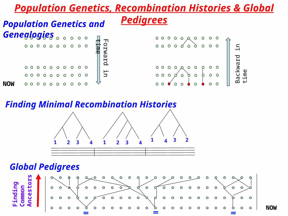
Population Genetics, Recombination Histories & Global Pedigrees

Finding Minimal Recombination Histories

1 2 3 4 1 2 3 4 1 234

Global Pedigrees

Fin

din

g

Co

mm

on

A

nc

es

tors

NOW

Population Genetics and Genealogies

NOW

Forw

ard in time

Bac

kwar

d in

tim

e

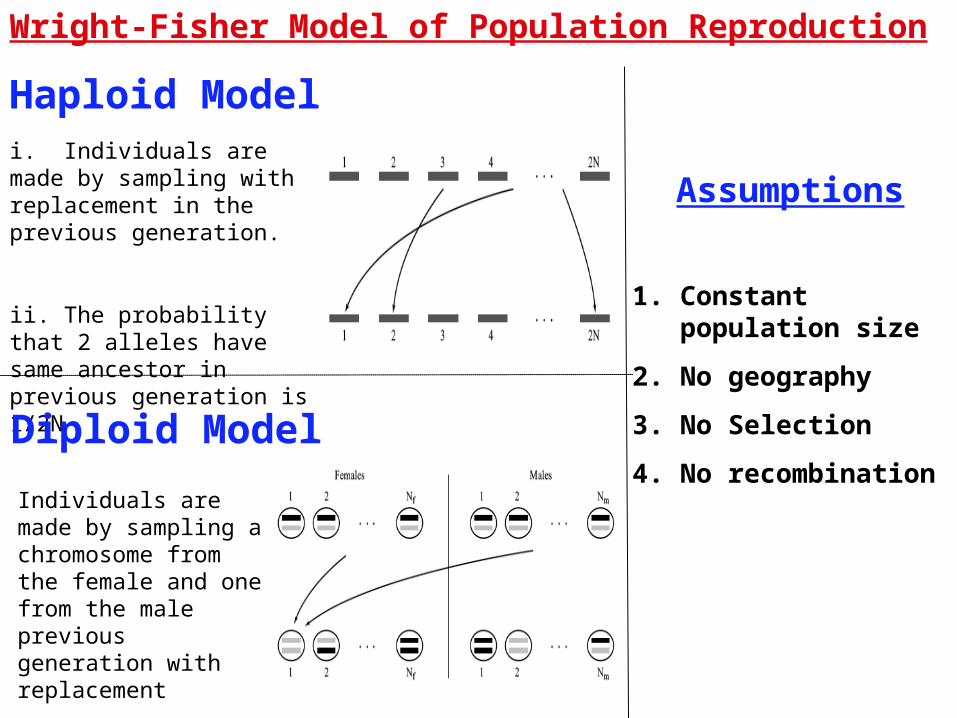
Wright-Fisher Model of Population Reproduction

Haploid Modeli. Individuals are made by sampling with replacement in the previous generation.

ii. The probability that 2 alleles have same ancestor in previous generation is 1/2N

Diploid Model

Individuals are made by sampling a chromosome from the female and one from the male previous generation with replacement

Assumptions

1. Constant population size

2. No geography

3. No Selection

4. No recombination

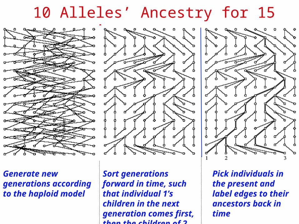
10 Alleles’ Ancestry for 15 generations

Generate new generations according to the haploid model

Sort generations forward in time, such that individual 1’s children in the next generation comes first, then the children of 2..

Pick individuals in the present and label edges to their ancestors back in time

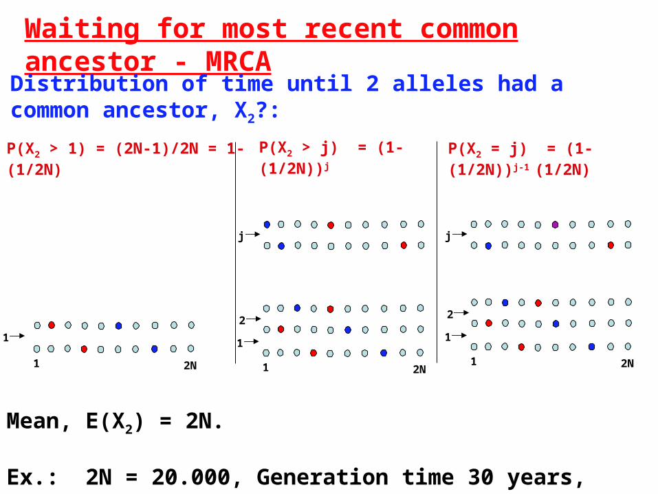
Mean, E(X2) = 2N.

Ex.: 2N = 20.000, Generation time 30 years, E(X2) = 600000 years.

Waiting for most recent common ancestor - MRCA

P(X2 = j) = (1-(1/2N))j-1 (1/2N)

Distribution of time until 2 alleles had a common ancestor, X2?:

P(X2 > j) = (1-(1/2N))jP(X2 > 1) = (2N-1)/2N = 1-(1/2N)

1 2N

1

1 2N

1

2

j

1 2N

1

2

j

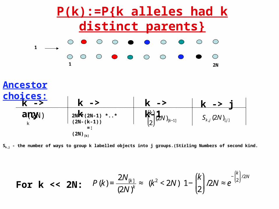
P(k):=P{k alleles had k distinct parents}

1 2N

1

(2N)k

k -> any2N *(2N-1) *..* (2N-(k-1)) =: (2N)[k]

k -> k

Ancestor choices:

k -> k-1

€

k

2

⎛

⎝ ⎜

⎞

⎠ ⎟(2N)[k−1]

€

P(k) =2N[k ]

(2N)k≈ (k 2 < 2N) 1−

k

2

⎛

⎝ ⎜

⎞

⎠ ⎟/2N ≈ e

−k

2

⎛

⎝ ⎜

⎞

⎠ ⎟/ 2N

For k << 2N:

k -> j

€

Sk, j (2N)[ j ]

Sk,j - the number of ways to group k labelled objects into j groups.(Stirling Numbers of second kind.

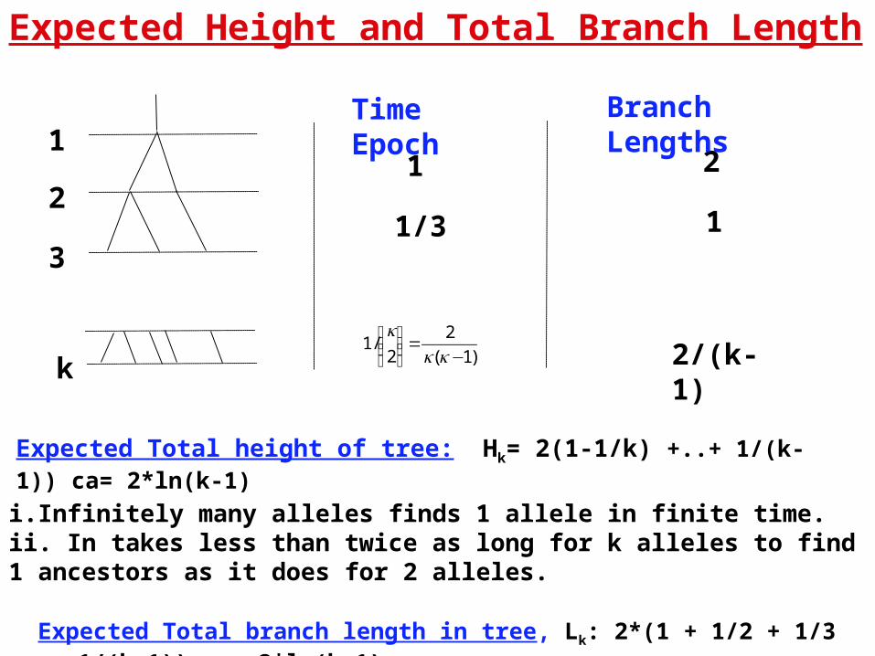
Expected Height and Total Branch Length

Expected Total height of tree: Hk= 2(1-1/k) +..+ 1/(k-1)) ca= 2*ln(k-1)

1

2

3

k

2

1

2/(k-1)

Branch Lengths

)1(

2

2/1

−=⎟⎟

⎠

⎞⎜⎜⎝

⎛kk

k

1/3

1

Time Epoch

i.Infinitely many alleles finds 1 allele in finite time.ii. In takes less than twice as long for k alleles to find 1 ancestors as it does for 2 alleles.

Expected Total branch length in tree, Lk: 2*(1 + 1/2 + 1/3 +..+ 1/(k-1)) ca= 2*ln(k-1)

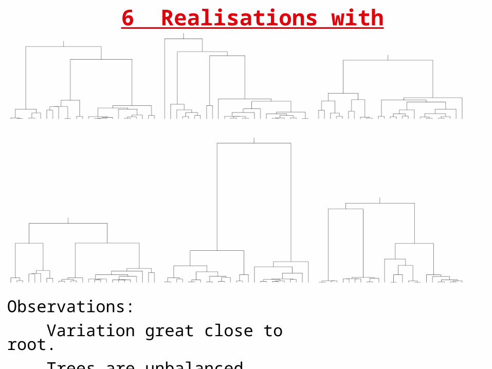
6 Realisations with 25 leaves

Observations:

Variation great close to root.

Trees are unbalanced.

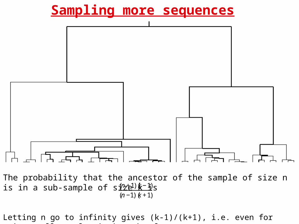
Sampling more sequences

The probability that the ancestor of the sample of size n is in a sub-sample of size k is

Letting n go to infinity gives (k-1)/(k+1), i.e. even for quite small samples it is quite large.

€

(n+1)(k−1)(n−1)(k+1)

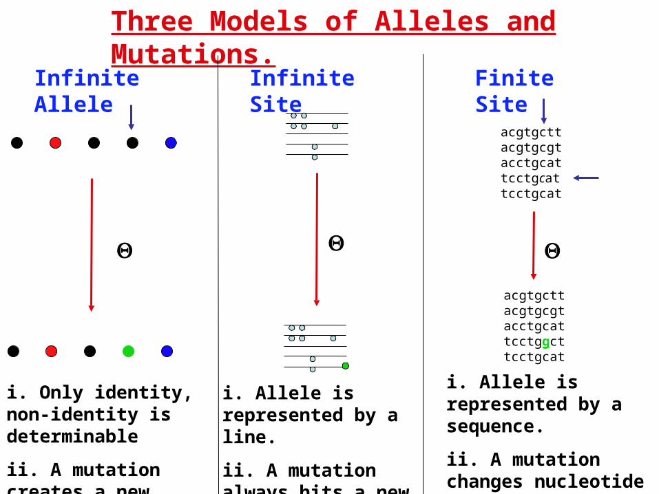
Three Models of Alleles and Mutations.

i. Only identity, non-identity is determinable

ii. A mutation creates a new type.

i. Allele is represented by a line.

ii. A mutation always hits a new position.

i. Allele is represented by a sequence.

ii. A mutation changes nucleotide at chosen position.

Infinite Allele

Infinite Site

Finite Site

acgtgcttacgtgcgtacctgcattcctgcattcctgcat

acgtgcttacgtgcgtacctgcattcctggcttcctgcat

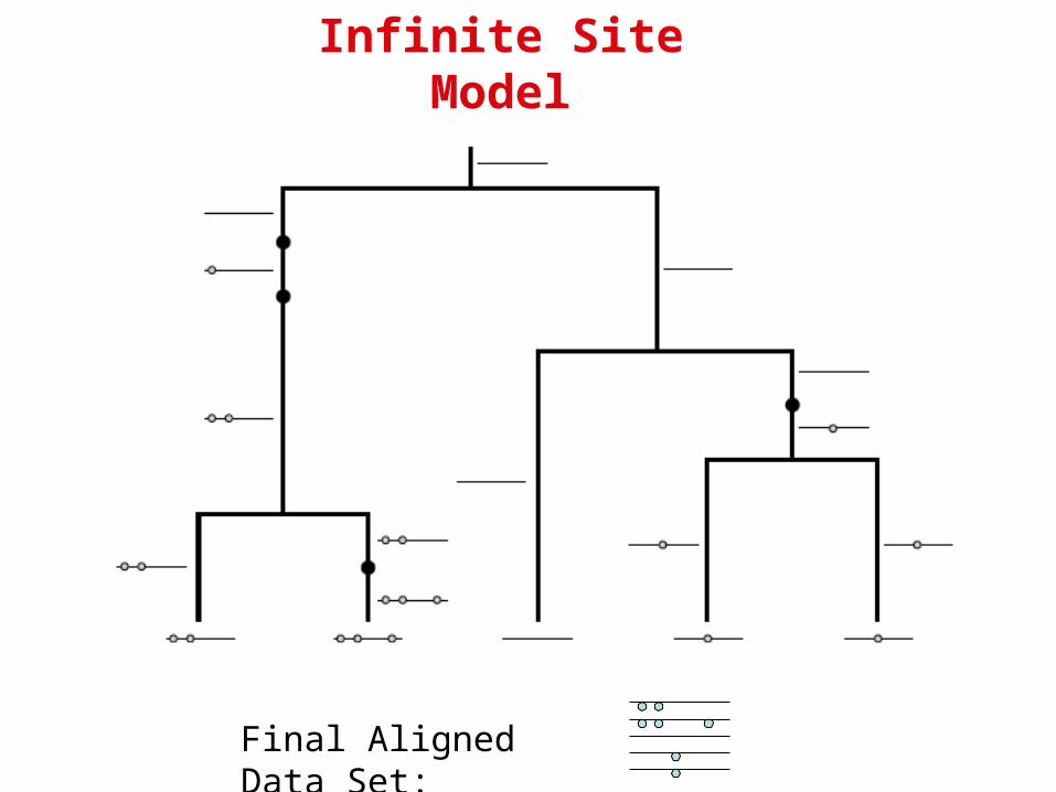
Final Aligned Data Set:

Infinite Site Model

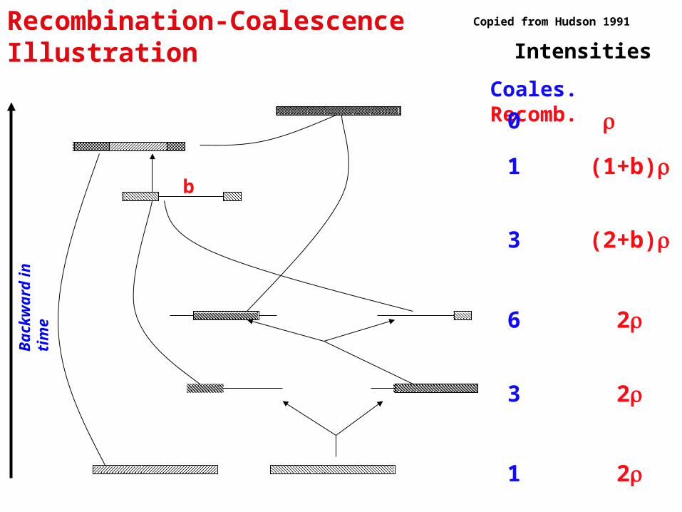
Recombination-Coalescence Illustration Copied from Hudson 1991

Intensities

Coales. Recomb.

1 2

3 2

6 2

1 (1+b)

0

3 (2+b)

b

Bac

kwar

d in

tim

e

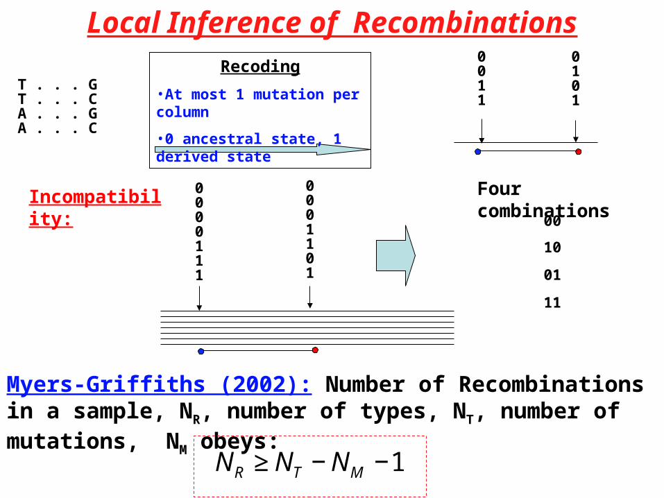
Local Inference of Recombinations

0000111

0001101

00

10

01

11

Four combinationsIncompatibility:

Myers-Griffiths (2002): Number of Recombinations in a sample, NR, number of types, NT, number of mutations, NM obeys:

€

NR ≥ NT − NM −1

0011

0101

T . . . GT . . . CA . . . GA . . . C

Recoding

•At most 1 mutation per column

•0 ancestral state, 1 derived state

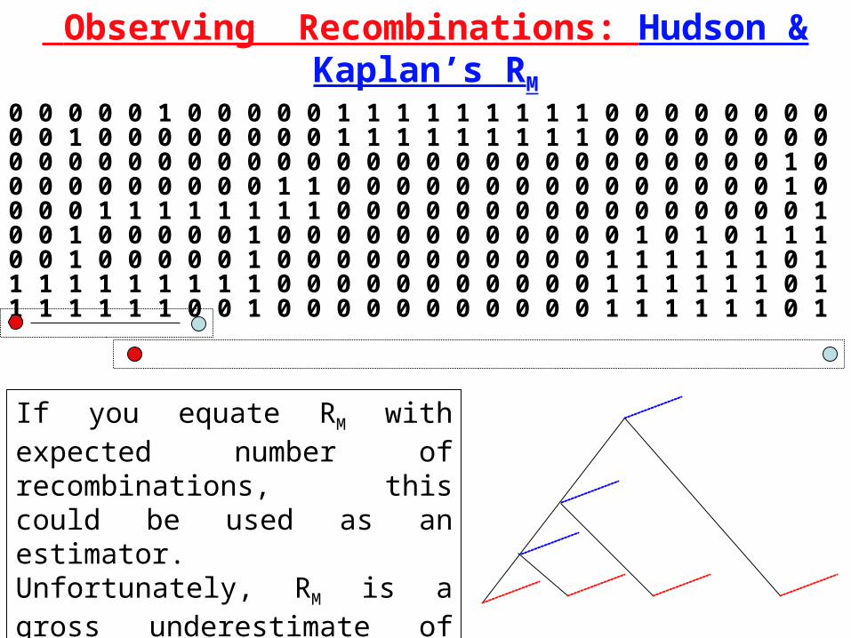
”Observing” Recombinations: Hudson & Kaplan’s RM

If you equate RM with expected number of recombinations, this could be used as an estimator. Unfortunately, RM is a gross underestimate of the real number of recombinations.

0 0 0 0 0 1 0 0 0 0 0 1 1 1 1 1 1 1 1 1 0 0 0 0 0 0 0 00 0 1 0 0 0 0 0 0 0 0 1 1 1 1 1 1 1 1 1 0 0 0 0 0 0 0 00 0 0 0 0 0 0 0 0 0 0 0 0 0 0 0 0 0 0 0 0 0 0 0 0 0 1 00 0 0 0 0 0 0 0 0 1 1 0 0 0 0 0 0 0 0 0 0 0 0 0 0 0 1 00 0 0 1 1 1 1 1 1 1 1 0 0 0 0 0 0 0 0 0 0 0 0 0 0 0 0 10 0 1 0 0 0 0 0 1 0 0 0 0 0 0 0 0 0 0 0 0 1 0 1 0 1 1 10 0 1 0 0 0 0 0 1 0 0 0 0 0 0 0 0 0 0 0 1 1 1 1 1 1 0 11 1 1 1 1 1 1 1 1 0 0 0 0 0 0 0 0 0 0 0 1 1 1 1 1 1 0 11 1 1 1 1 1 0 0 1 0 0 0 0 0 0 0 0 0 0 0 1 1 1 1 1 1 0 1

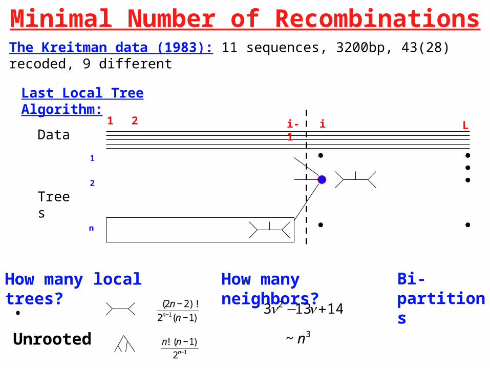
Minimal Number of Recombinations

Last Local Tree Algorithm:

L21Data

2

n

i-1 i

1

Trees

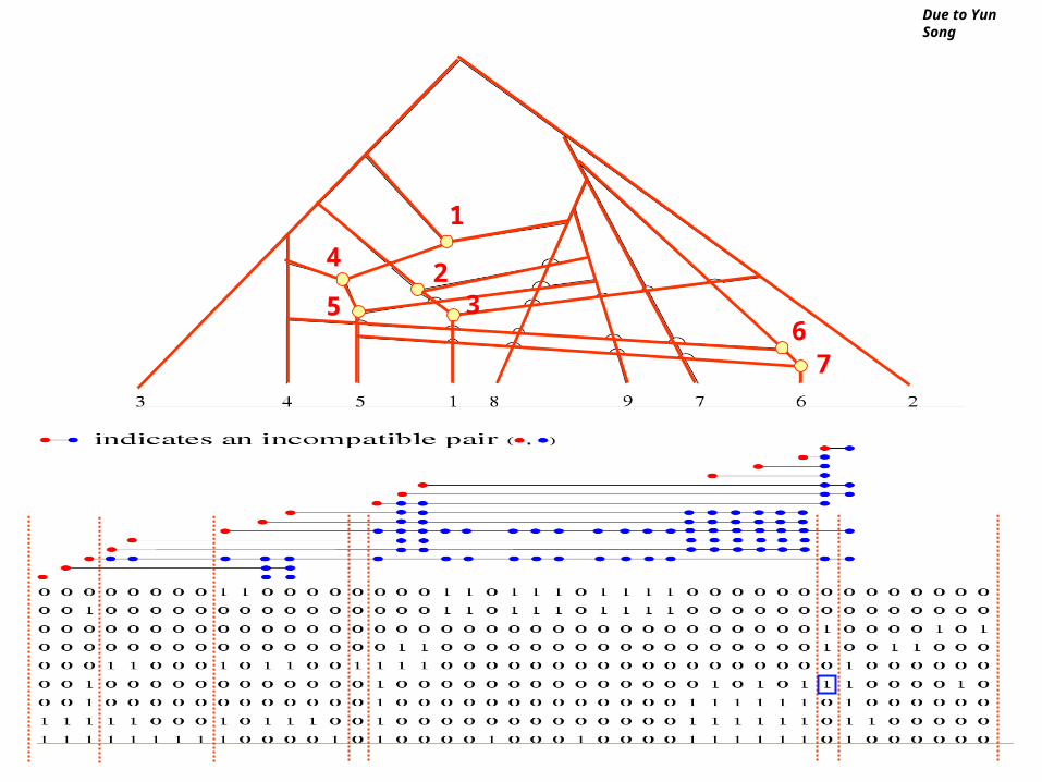
The Kreitman data (1983): 11 sequences, 3200bp, 43(28) recoded, 9 different

How many neighbors?

€

(2n − 2)!

2n−1(n −1)!

€

n! (n −1)!

2n−1

14133 2 +− nn

€

~ n3

Bi-partitionsHow many local trees?

• Unrooted

• Coalescent

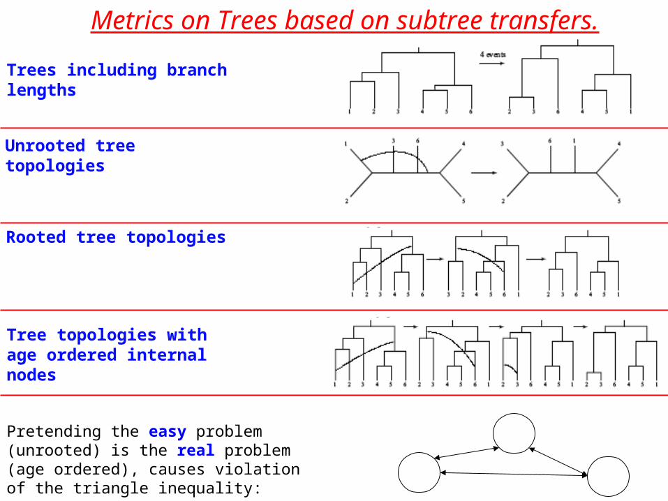
Metrics on Trees based on subtree transfers.

Pretending the easy problem (unrooted) is the real problem (age ordered), causes violation of the triangle inequality:

Tree topologies with age ordered internal nodes

Rooted tree topologies

Unrooted tree topologies

Trees including branch lengths

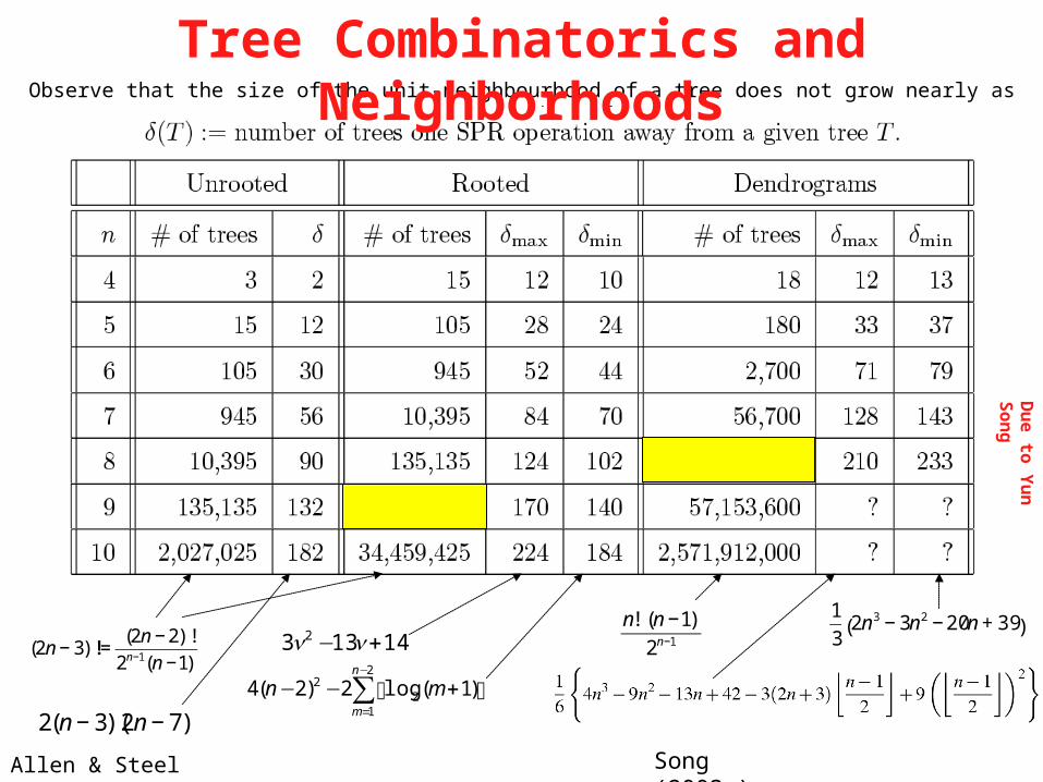
Observe that the size of the unit-neighbourhood of a tree does not grow nearly as fast as the number of trees

Allen & Steel (2001) Song (2003+)

Du

e to Yu

n S

ong

Tree Combinatorics and Neighborhoods

€

1

32n3 − 3n2 − 20n + 39( )

€

n! (n −1)!

2n−1

€

(2n − 3)!!=(2n − 2)!

2n−1(n −1)!

⎣ ⎦∑−

=

+−−2

12

2 )1(log2)2(4n

m

mn

14133 2 +− nn

€

2(n − 3)(2n − 7)

1

23

4

56

7

Due to Yun Song

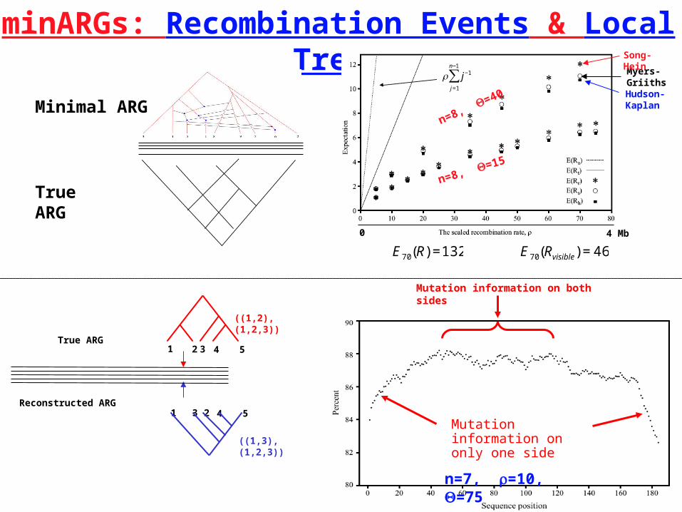
minARGs: Recombination Events & Local Trees

True ARG

Reconstructed ARG

1 2 3 4 5

1 23 4 5

((1,2),(1,2,3))

((1,3),(1,2,3))

n=7, =10, =75

Minimal ARG

True ARG

Mutation information on only one side

Mutation information on both sides

0 4 Mb

Hudson-Kaplan

Myers-Griiths

Song-Hein

n=8, =40

n=8, =15

€

j−1

j=1

n−1

∑

€

E70(R) =132

€

E70(Rvisible ) = 46

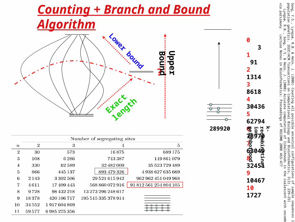
Counting + Branch and Bound Algorithm

?

Exact len

gth

Lower bound

Up

per B

oun

d

0 31 912 13143 86184 304365 627946 789707 630498 324519 1046710 1727

289920

k-recom

bin

atination

n

eighb

orhood

k

Song, Y

.S., Lyngsø, R

.B. &

Hein, J. (2006) C

ounting all possible ancestral configurations of sample sequences in population genetics. IE

EE

/AC

M T

ransactions on C

omputational B

iology and Bioinform

atics, 3(3), 239–251 Lyngsø, R

.B., S

ong, Y.S

. & H

ein, J. (2008) Accurate com

putation of likelihoods in the coalescent w

ith recombination via parsim

ony. Lecture N

otes in Bioinform

atics: Proceedings of RE

CO

MB

2008 463–477

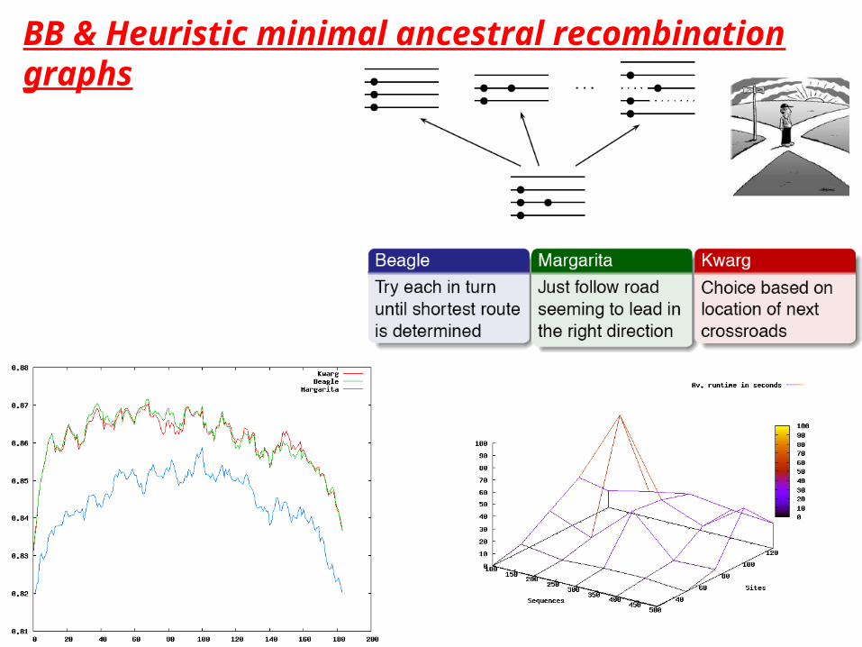
BB & Heuristic minimal ancestral recombination graphs

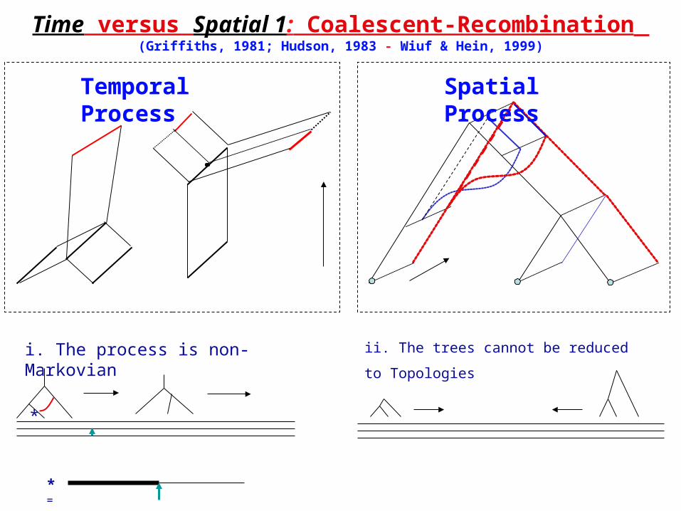
Time versus Spatial 1: Coalescent-Recombination (Griffiths, 1981; Hudson, 1983 - Wiuf & Hein, 1999)

Temporal Process Spatial Process

ii. The trees cannot be reduced to Topologies i. The process is non-Markovian

*

* =

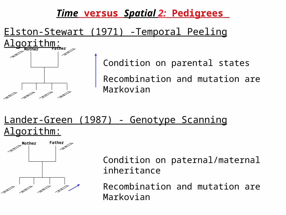
Elston-Stewart (1971) -Temporal Peeling Algorithm:

Lander-Green (1987) - Genotype Scanning Algorithm:

Mother Father

Condition on parental states

Recombination and mutation are Markovian

Mother Father

Condition on paternal/maternal inheritance

Recombination and mutation are Markovian

Time versus Spatial 2: Pedigrees

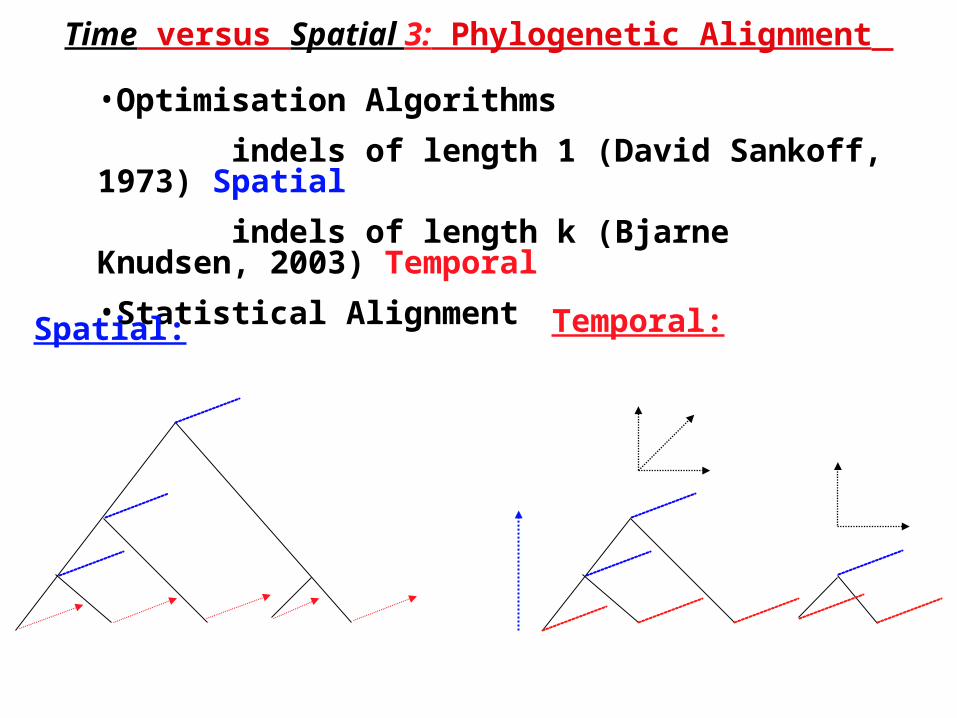
Time versus Spatial 3: Phylogenetic Alignment

•Optimisation Algorithms

indels of length 1 (David Sankoff, 1973) Spatial

indels of length k (Bjarne Knudsen, 2003) Temporal

•Statistical Alignment

Spatial: Temporal:

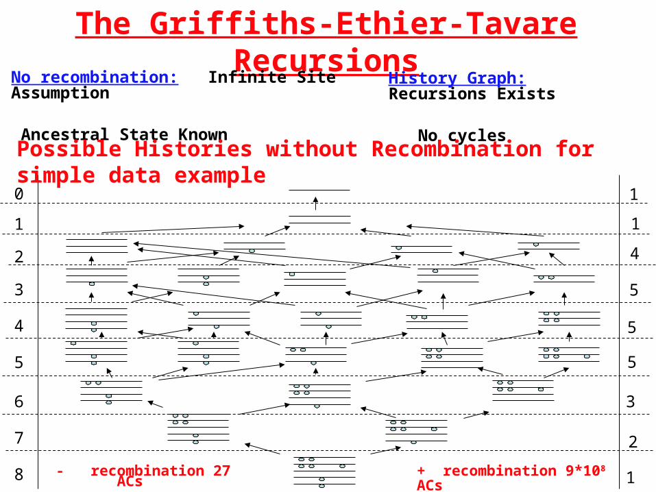
- recombination 27 ACs

0

1

2

3

4

5

6

7

8

1

1

4

2

5

3

1

5

5

The Griffiths-Ethier-Tavare Recursions

No recombination: Infinite Site Assumption

Ancestral State Known

History Graph: Recursions Exists

No cycles

Possible Histories without Recombination for simple data example

+ recombination 9*108 ACs

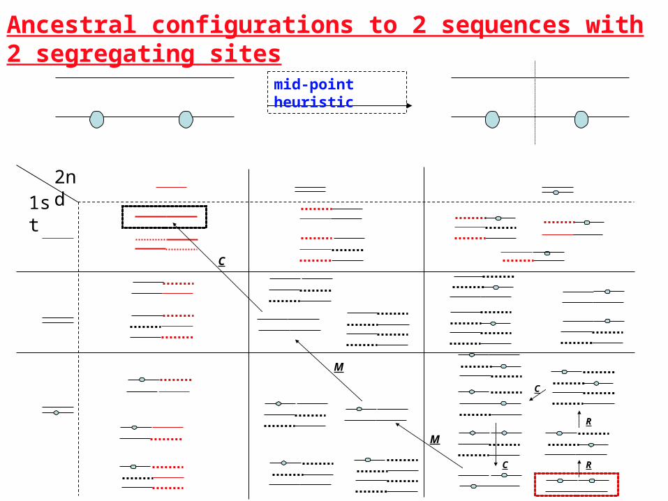
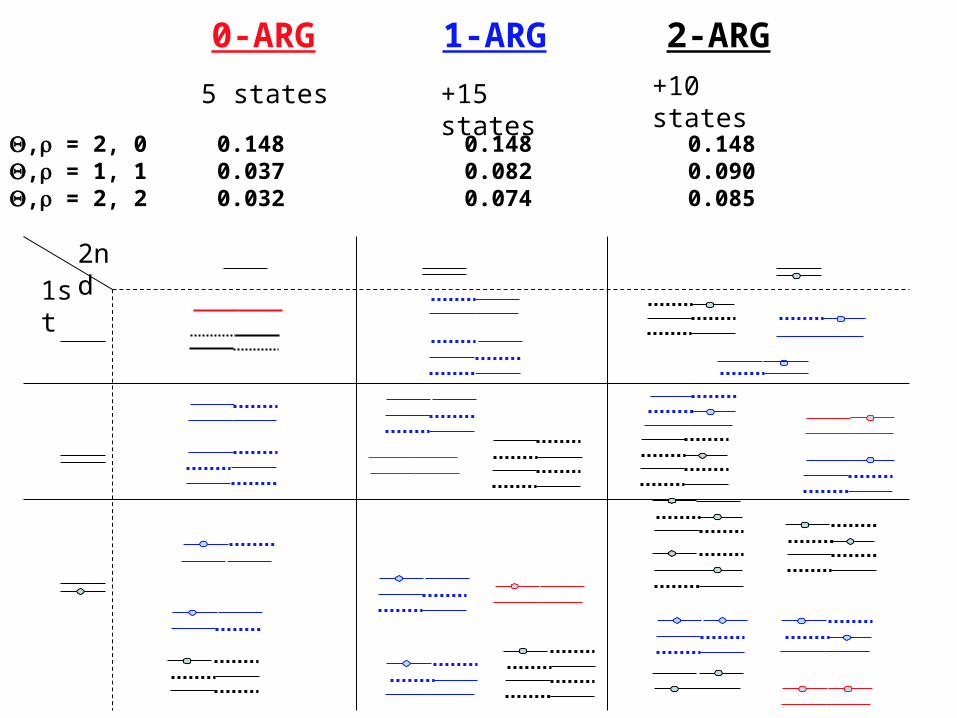
1st

2nd

Ancestral configurations to 2 sequences with 2 segregating sites

mid-point heuristic

M

M

R

C

R

C

C

1st

2nd

0-ARG

5 states

1-ARG

+15 states

2-ARG

+10 states

, = 2, 0, = 1, 1, = 2, 2

0.1480.0370.032

0.1480.0820.074

0.1480.0900.085

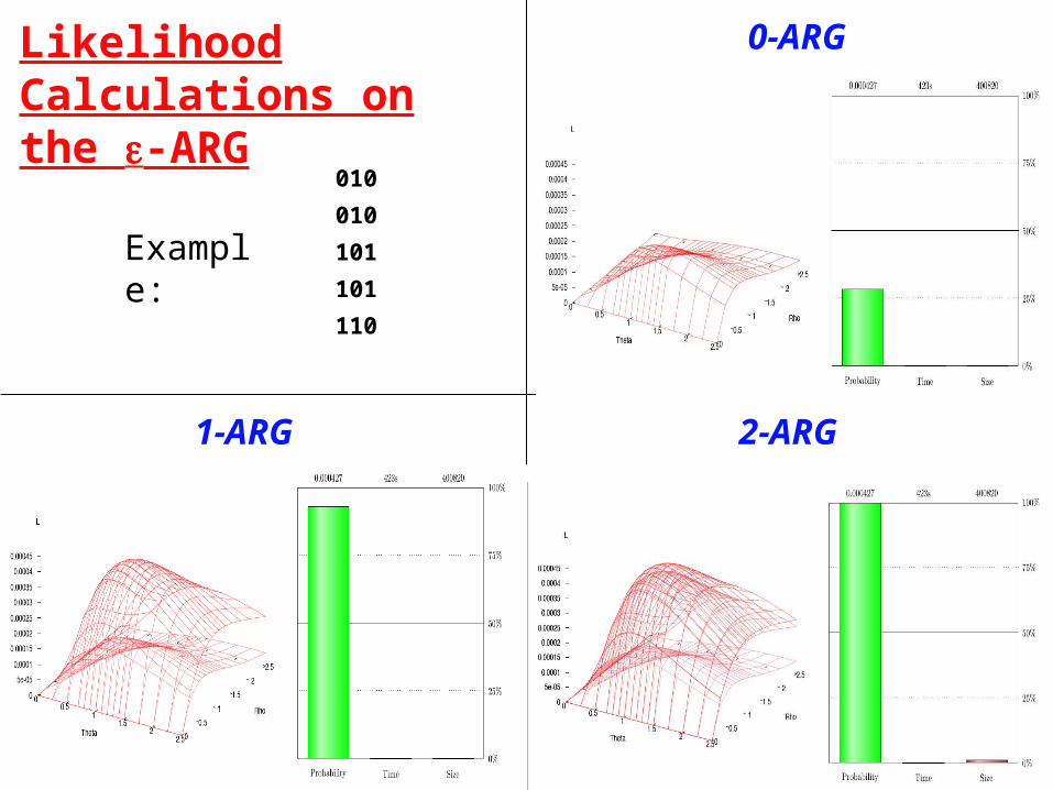
Likelihood Calculations on the -ARG

010

010

101

101

110

Example:

0-ARG

2-ARG1-ARG

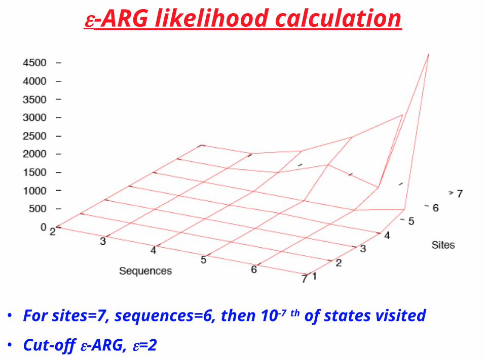
• For sites=7, sequences=6, then 10-7 th of states visited

• Cut-off -ARG, =2

-ARG likelihood calculation

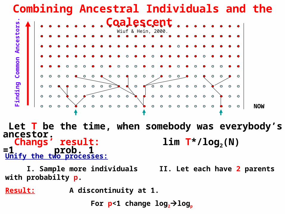
Combining Ancestral Individuals and the Coalescent Wiuf & Hein, 2000.

Let T be the time, when somebody was everybody’s ancestor.

Fin

din

g C

om

mo

n A

nc

es

tors

.

NOW

Changs’ result: lim T*/log2(N) =1 prob. 1

Unify the two processes:

I. Sample more individuals II. Let each have 2 parents with probabilty p.

Result: A discontinuity at 1.

For p<1 change log2logp

Comment: Genetic Ancestors is a vanishing set within Genealogical Ancestors.

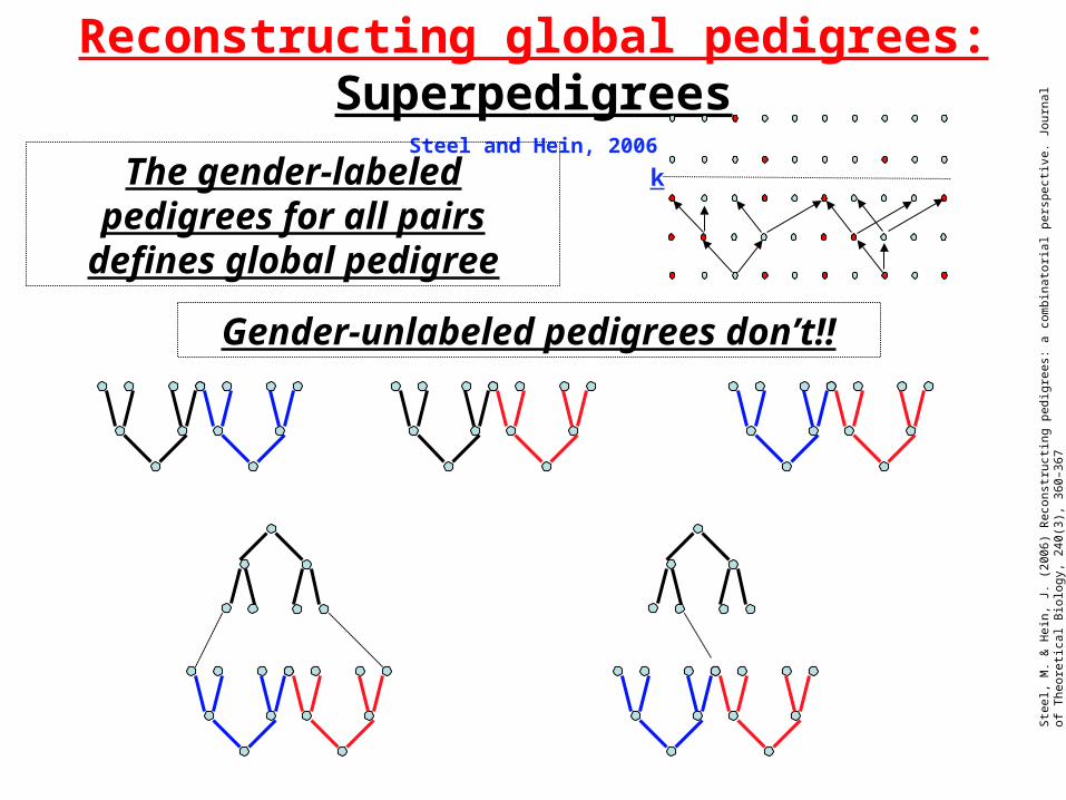
Reconstructing global pedigrees: SuperpedigreesSteel and Hein, 2006

The gender-labeled pedigrees for all pairs defines global pedigree

k

Gender-unlabeled pedigrees don’t!!

Ste

el, M

. & H

ein,

J. (

2006

) R

econ

stru

ctin

g pe

digr

ees:

a c

ombi

nato

rial

per

spec

tive

. Jou

rnal

of

The

oret

ical

Bio

logy

, 240

(3),

360

–367

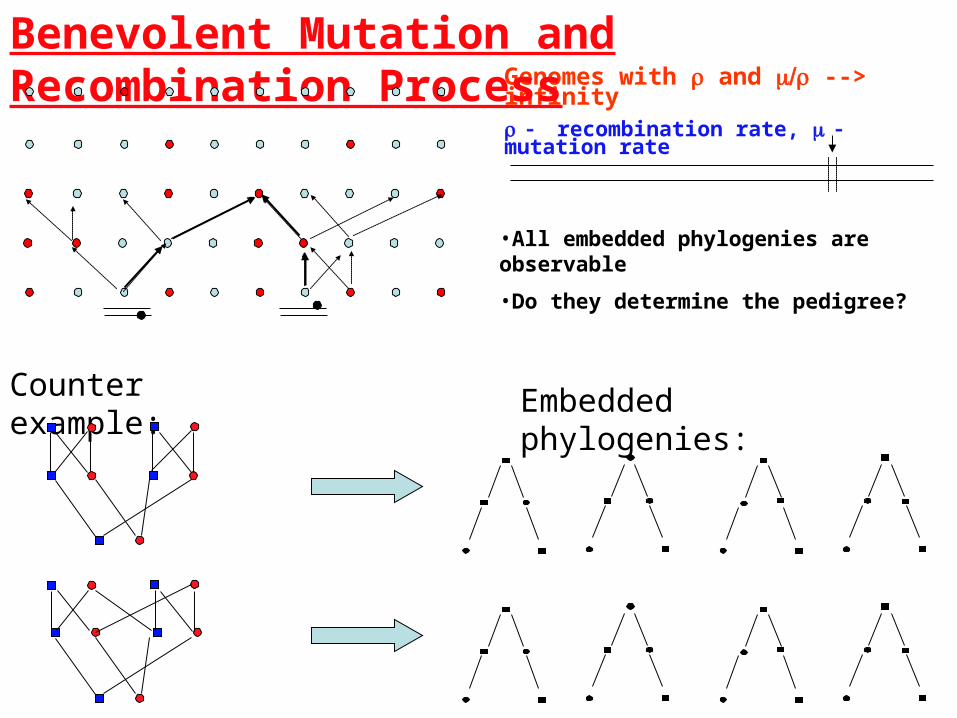
•All embedded phylogenies are observable

•Do they determine the pedigree?

Genomes with and --> infinity recombination rate, mutation rate

Benevolent Mutation and Recombination Process

Counter example: Embedded phylogenies:

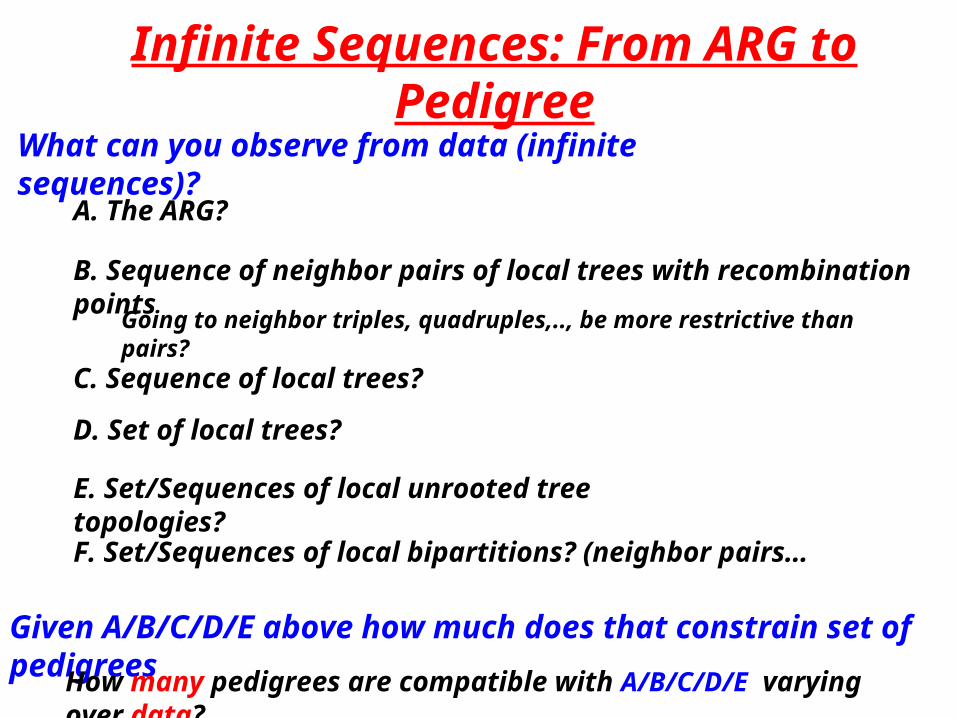
Infinite Sequences: From ARG to Pedigree

Given A/B/C/D/E above how much does that constrain set of pedigrees

How many pedigrees are compatible with A/B/C/D/E varying over data?

A. The ARG?

What can you observe from data (infinite sequences)?

C. Sequence of local trees?

D. Set of local trees? E. Set/Sequences of local unrooted tree topologies?

B. Sequence of neighbor pairs of local trees with recombination points

Going to neighbor triples, quadruples,.., be more restrictive than pairs?

F. Set/Sequences of local bipartitions? (neighbor pairs…

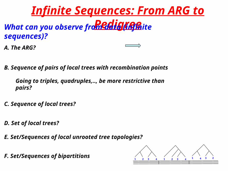
Infinite Sequences: From ARG to Pedigree

A. The ARG?

What can you observe from data (infinite sequences)?

C. Sequence of local trees?

D. Set of local trees? E. Set/Sequences of local unrooted tree topologies?

B. Sequence of pairs of local trees with recombination points

Going to triples, quadruples,.., be more restrictive than pairs?

1 2 3 4 1 2 3 4 1 234F. Set/Sequences of bipartitions