Embed Size (px)
DESCRIPTION
Geometric Dimensioning and Tolerancing
Citation preview
1
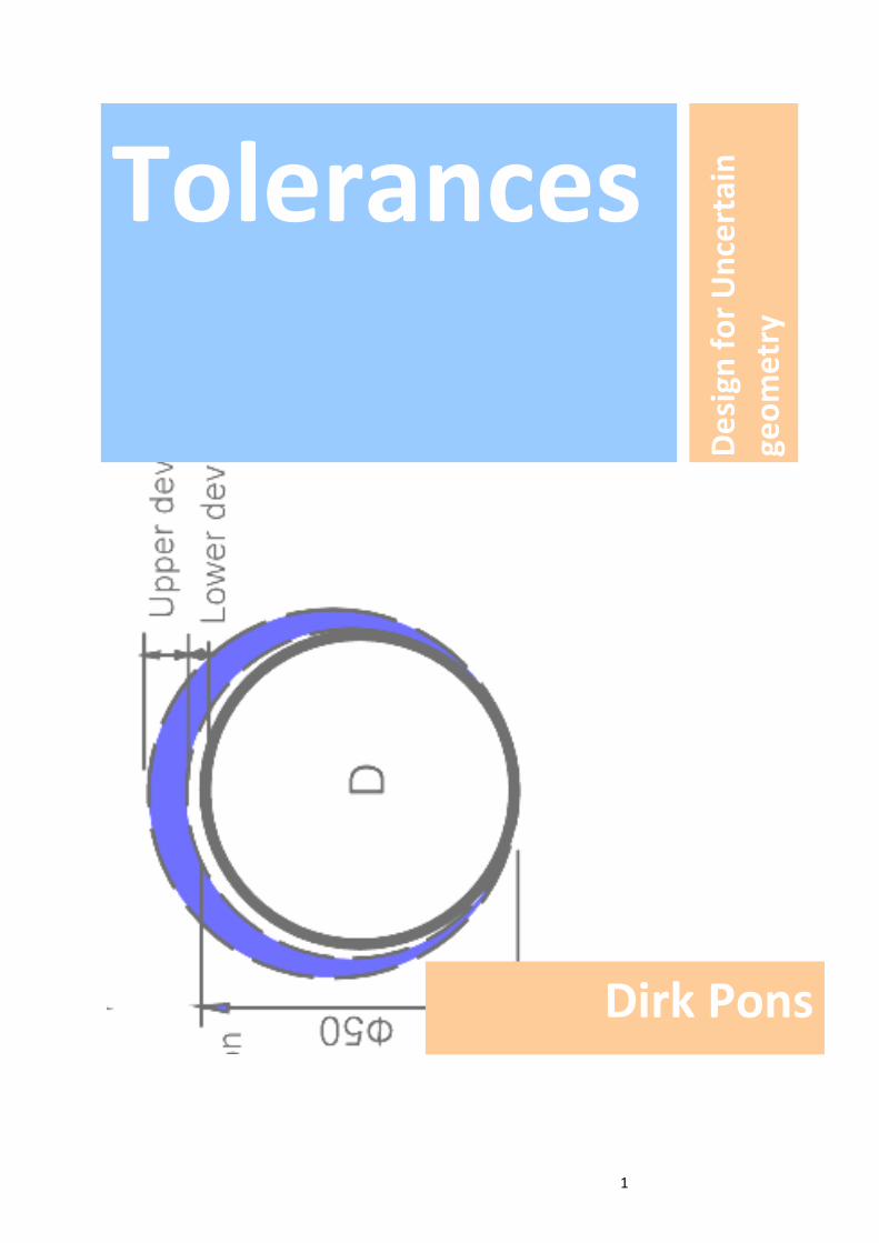
Tolerances
Dirk Pons
De
sig
n f
or
Un
cert
ain
ge
om
etr
y
2
Tolerances • Limits and fits in
engineering
design
• Linear tolerances
• Geometric
tolerances
Dirk Pons has a PhD in mechanical
engineering and several years
industrial experience in design and
manufacturing, with a special
emphasis on new product
development. He was a member of the
team that designed the Fisher + Paykel
‘DishDrawer’, an innovative
dishwasher. He has also taught
engineering and is currently a senior
lecturer at the University of
Canterbury. This booklet on tolerances
is an extract from his lecturing notes
on engineering design.
Please address correspondence to Dr
Dirk Pons, Department of Mechanical
Engineering, University of Canterbury,
Private Bag 4800, Christchurch 8020,
New Zealand, Email:
Copyright D Pons 1997-2012.
Document and revision:
Pons_MED03_Tolerances_E4.12.doc
Tolerances are used in
engineering design to make sure
that the parts of an assembly go
together with the correct amount
of looseness or tightness. This is
important because functionality
of the system depends on the
behaviour at the interface of the
parts. Designers therefore
convert the functional
requirements into tolerances,
which are then used in the
manufacture of the part.
3
1 General tolerances
This paper summarises the application of general tolerances and surface
texture for engineering design and production engineering.
1.1 Tolerances - adding value to design
One of the most important parts of design is the selection of tolerances.
Tolerances are shown in the example of the detailed shaft drawing a few
pages back, by the ± terms in the dimensions. The tolerance tells the
fabricator what range of size is acceptable. This sounds simple, and it is,
but it has profound consequences. For a start, the tolerance affects
function. A shaft that is too large is going to be too tight in the bearing: it
might not go in at all, or it might go in but overheat the bearing during
service. Therefore the designer generally has to keep part tolerances
small, so that the required function is obtained. On the other hand,
generous tolerances make fabrication easier, quicker and cheaper. When
tolerances are close, then the work becomes “precision engineering” and
the costs go up. All that lies between precision and plain engineering is a
few symbols from the designer.
Balancing function and cost
Therefore there are two opposing forces on tolerances, and the balance
has to be determined by the designer. The determination of suitable
tolerances is probably the most important aspect of detailed design,
because of their effect on production cost and function. Tolerances should
be first be selected on the basis of product function, and next on the basis
of lowering the cost. Generally it is possible to limit the tight tolerances to
a few sensitive dimensions which contribute most to function of the
product. Insensitive dimensions may be relaxed.
The designer needs to take particular care with tolerances where parts or
assemblies mate (e.g. a motor to a gearbox), especially if parts are to be
interchangeable. Fits, such as loose running bearings through to tight
interference fits, also need attention from the designer. There are three
different types of tolerance that the designer can apply to a drawing, and
these are Tolerances, Geometric Tolerances, and Fits. These are so
important that they have been given their own sections following.
Essentially a dimension is incomplete without a tolerance. Of all your
design work, the tolerances are the part your competitors would want to
get their hands on. Almost all the rest they can get from measuring up.
The tolerances are the link between ease of fabrication and adequate
function.
4
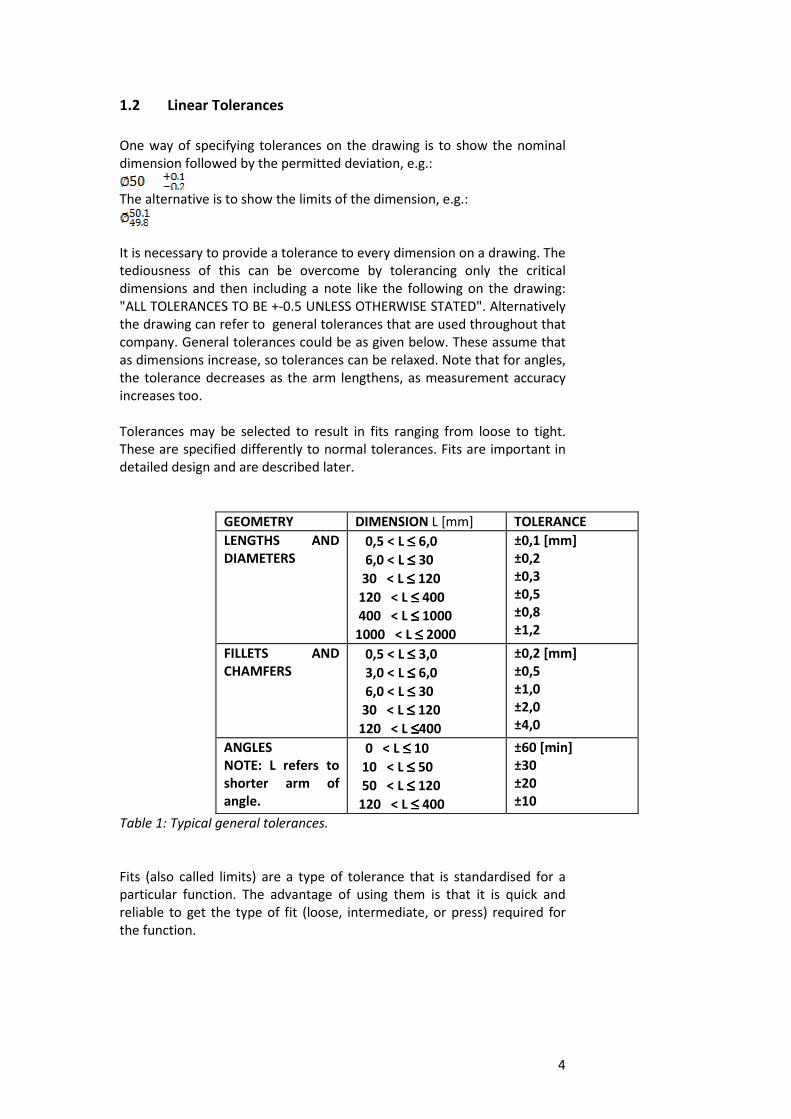
1.2 Linear Tolerances
One way of specifying tolerances on the drawing is to show the nominal
dimension followed by the permitted deviation, e.g.:
The alternative is to show the limits of the dimension, e.g.:
It is necessary to provide a tolerance to every dimension on a drawing. The
tediousness of this can be overcome by tolerancing only the critical
dimensions and then including a note like the following on the drawing:
"ALL TOLERANCES TO BE +-0.5 UNLESS OTHERWISE STATED". Alternatively
the drawing can refer to general tolerances that are used throughout that
company. General tolerances could be as given below. These assume that
as dimensions increase, so tolerances can be relaxed. Note that for angles,
the tolerance decreases as the arm lengthens, as measurement accuracy
increases too.
Tolerances may be selected to result in fits ranging from loose to tight.
These are specified differently to normal tolerances. Fits are important in
detailed design and are described later.
GEOMETRY DIMENSION L [mm] TOLERANCE
LENGTHS AND
DIAMETERS
0,5 < L ≤≤≤≤ 6,0
6,0 < L ≤≤≤≤ 30
30 < L ≤≤≤≤ 120
120 < L ≤≤≤≤ 400
400 < L ≤≤≤≤ 1000
1000 < L ≤≤≤≤ 2000
±0,1 [mm]
±0,2
±0,3
±0,5
±0,8
±1,2
FILLETS AND
CHAMFERS
0,5 < L ≤≤≤≤ 3,0
3,0 < L ≤≤≤≤ 6,0
6,0 < L ≤≤≤≤ 30
30 < L ≤≤≤≤ 120
120 < L ≤≤≤≤400
±0,2 [mm]
±0,5
±1,0
±2,0
±4,0
ANGLES
NOTE: L refers to
shorter arm of
angle.
0 < L ≤≤≤≤ 10
10 < L ≤≤≤≤ 50
50 < L ≤≤≤≤ 120
120 < L ≤≤≤≤ 400
±60 [min]
±30
±20
±10
Table 1: Typical general tolerances.
Fits (also called limits) are a type of tolerance that is standardised for a
particular function. The advantage of using them is that it is quick and
reliable to get the type of fit (loose, intermediate, or press) required for
the function.
5
2 Surface texture
Surface texture refers to the (microscopic) roughness of the surface. The
roughness is measured with a stylus, and commonly expressed as the
verage height above the centre line (“centre line average”, or arithmetical
mean deviation”), and given the symbol Ra. Surface texture will need to be
specified where the normal machining processes are unlikely to give an
acceptable surface. The symbol used for surface texture s the shown in the
figure below.
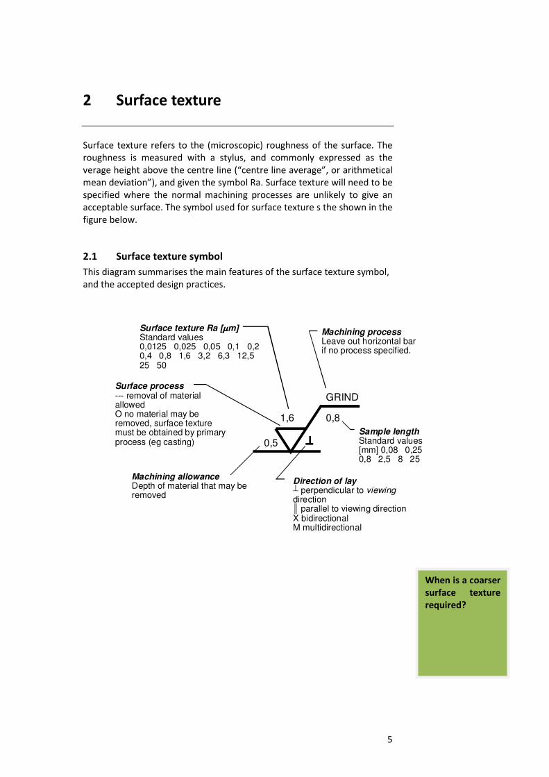
2.1 Surface texture symbol
This diagram summarises the main features of the surface texture symbol,
and the accepted design practices.
1,6
GRIND
0,8
0,5
Surface texture Ra [::::m]Standard values0,0125 0,025 0,05 0,1 0,20,4 0,8 1,6 3,2 6,3 12,5 25 50
Machining processLeave out horizontal barif no process specified.
Sample lengthStandard values[mm] 0,08 0,25 0,8 2,5 8 25
Direction of lay2 perpendicular to viewingdirection5 parallel to viewing directionX bidirectionalM multidirectional
Surface process--- removal of materialallowedO no material may beremoved, surface texturemust be obtained by primaryprocess (eg casting)
Machining allowanceDepth of material that may beremoved
When is a coarser
surface texture
required?
6
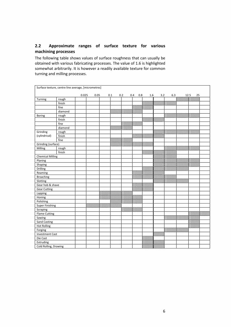
2.2 Approximate ranges of surface texture for various
machining processes
The following table shows values of surface roughness that can usually be
obtained with various fabricating processes. The value of 1.6 is highlighted
somewhat arbitrarily. It is however a readily available texture for common
turning and milling processes.
Surface texture, centre line average, [micrometres]
0.025 0.05 0.1 0.2 0.4 0.8 1.6 3.2 6.3 12.5 25
Turning rough
finish
fine
diamond
Boring rough
finish
fine
diamond
rough
finish
Grinding
(cylindrical)
fine
Grinding (surface)
Milling rough
finish
Chemical Milling
Planing
Shaping
Drilling
Reaming
Broaching
Slotting
Gear hob & shave
Gear Cutting
Lapping
Honing
Polishing
Super Finishing
Scraping
Flame Cutting
Sawing
Sand Casting
Hot Rolling
Forging
Investment Cast
Die Cast
Extruding
Cold Rolling, Drawing
7
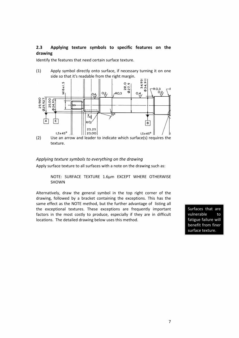
2.3 Applying texture symbols to specific features on the
drawing
Identify the features that need certain surface texture.
(1) Apply symbol directly onto surface, if necessary turning it on one
side so that it's readable from the right margin.
(2) Use an arrow and leader to indicate which surface(s) requires the
texture.
Applying texture symbols to everything on the drawing
Apply surface texture to all surfaces with a note on the drawing such as:
NOTE: SURFACE TEXTURE 1.6μm EXCEPT WHERE OTHERWISE
SHOWN
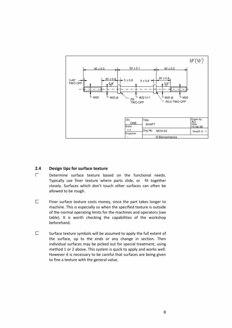
Alternatively, draw the general symbol in the top right corner of the
drawing, followed by a bracket containing the exceptions. This has the
same effect as the NOTE method, but the further advantage of listing all
the exceptional textures. These exceptions are frequently important
factors in the most costly to produce, especially if they are in difficult
locations. The detailed drawing below uses this method.
Surfaces that are
vulnerable to
fatigue failure will
benefit from finer
surface texture.
8
© Biomechanics
Drg No.
Title:
Projection
Qty
Sheet of
Drawn by:
Date:Scale
SHAFT
MCH-02
ONE
1:1
-
1 1
AO
15-06-95
40 ± 0,5 50 ± 0,1 40 ± 0,5
20 ± 0,8 20 ± 0,85 ± 0,8 5 ± 0,81x45E
TWO OFF
M20M20 j6
R0,5 TWO OFF
M22 h11M20 j6M20
0,40,8
0,40,4
R5TWO OFF
2.4 Design tips for surface texture ☐ Determine surface texture based on the functional needs.
Typically use finer texture where parts slide, or fit together
closely. Surfaces which don’t touch other surfaces can often be
allowed to be rough.
☐ Finer surface texture costs money, since the part takes longer to
machine. This is especially so when the specified texture is outside
of the normal operating limits for the machines and operators (see
table). It is worth checking the capabilities of the workshop
beforehand.
☐ Surface texture symbols will be assumed to apply the full extent of
the surface, up to the ends or any change in section. Then
individual surfaces may be picked out for special treatment, using
method 1 or 2 above. This system is quick to apply and works well.
However it is necessary to be careful that surfaces are being given
to fine a texture with the general value.
9
3 Limits and fits
Abstract
Tolerances are used in engineering design to make sure that the parts of
an assembly go together with the correct amount of looseness or
tightness. The design intent is for a certain type of fit, and tolerances
provide the designer with a mechanism to ensure that is obtained, even if
the parts are made in large volumes. This paper describes the application
of limits and fits for engineering design and production engineering.
3.1 Introduction
Fits (also called limits) are a type of tolerance that is standardised for a
particular function. The advantage of using them is that it is quick and
reliable to get the type of fit (loose, intermediate, or press) required for
the function.
The problem with manufacturing any assembly in volumes is that of
variable dimensions. The parts cannot be produced exactly identical: there
will always be some dimensional variability. Consequently, when parts are
mated together, e.g. a shaft is assembled into a bearing, it is possible that
the dimensions clash. If the assembly was expected to be an easy mating,
then it is possible that the dimensions of the parts might make this
difficult: either a shaft that is too large, or a hole that is too small, or
combinations thereof.
If only one assembly is being made, then it is a simple matter of
craftsmanship to manually sandpaper the shaft down to the right size or
do whatever else is necessary to fix the problem (fixing too loose a fit is a
fiddly job often involving making up sleeve inserts). Such fixes are possible
but they are uneconomical in volume production. We have to find a better
way.
The need for tolerances
The ideal is that any shaft that comes off the production line be able to be
fitted with any hole part (e.g. bearing). That would give us maximum
interchangeablility of parts. That is also important from a service and
maintenance perspective.
Therefore it is necessary to limit the variability of the mating features on
both the shaft and the hole. We do this by setting a tolerance on the
relevant dimensions.
The tolerance is an instruction on the drawing, giving the maximum and
minimum permissible deviations in size from the nominal dimension. For
example, a hole may be permitted to range in size from 49.5 mm to 50.2
Fits may be
applied to any
mating parts,
including shaft-
hole, key-keyway,
and any other
features that
mate.
10
mm, in which case the dimension on the drawing would be expressed as
φ50+0.2 - 0.5
Cost of tight tolerances
The tighter the tolerance, the better the interchangeability of parts.
However tight tolerances also cost a lot more to produce. So we also need
to relax the tolerances as much as possible, to reduce manufacturing cost.
How much is enough?
Types of fit
There is another problem too: we have a need for different types of fit,
from loose to tight. When we want loose fits, they must all be loose, and
when we want tight fits they must all be tight.
Typical assembly functions range from loosely running plain bearings to
tight press fits. Tolerances may be used for these assemblies, but it is more
convenient to use standard tolerances, which are called fits (or limits).
So we need a way to determine how much tolerances to set to give us the
required functionality. This can be calculated based on structural
mechanics, but it is a slow process that has to be repeated for every
design, and over the years Engineers have developed a very much faster
method, one that solves all the above problems, and is easy to use. It is
called 'fits', and it uses a special code. The process starts with the
Designer.
3.2 Designing with fits
The choice of tolerances is the designer's decision, and usually takes into
account:
* the intended function of the part
* the available manufacturing facilities
* the cost implications
Selecting the fit is easy: just find a combination from one of the known-
good fits (preferred) below, and note the two codes.
Preferred fits
There are some fit combinations that have been found work well, and
these are called preferred fits. They are listed below.
Clearance fits
Hole Shaft
H11 c11 SLACK RUNNING FIT. Wide commercial tolerance, external
members. Used on agricultural bearings. Shaft Alternative: C11-h11.
Finer grades are also used, e.g. H7-c8.
H9 d9 LOOSE RUNNING FIT. Suitable for large heavy journal bearing loads,
high speeds, large temperature fluctuations. Axial location accuracy
is poor. Also used for loose pulleys. Alternatively H7-d8, H8-d8,
Shaft D9-h9.
H9 e8 FREE RUNNING FIT. For moderate speeds and journal pressures.
Provides better accuracy. Alternatively H8-f7, H7-e8, H6-e7. Finer
“Hole” may also
be applied to
keyways, and any
other geometry
which has an
internal
dimension
11
grades are used for bearings of internal combustion engine (main ~,
camshaft ~, rocker arm ~). Shaft F8-h7
H8 f7 NORMAL RUNNING FIT. Commonly used fit for rotation, with good
accuracy. Used on plain bearings for gear box and pump.
Alternatives H8-f8, H7-f7, H6-f6
H7 g6 SLIDING FIT. Locates accurately, and turns freely, but not intended
for continuous running (except under light loads). Used for spigots
for location. Alternative fits H6-g5. Shaft G7-h6.
Transition fits
Hole Shaft
H7 h6 LOCATION-CLEARANCE FIT. Close fit for stationary parts, suitable for
easy assembly and disassembly. Unsuited to continuous running. A
small clearance will usually, but not necessarily, be present.
Alternatives H8-h7, H11-h11, H7-h5. Shaft H7-h6.
H7 js6 LOCATION-TRANSITION FIT. Provides accurate, tight, stationary
location. A small clearance will usually, but not necessarily, be
present. Used for spigots, ring gears in hubs. Alternatives H8-js7,H6-
js5, H7-k6, Shaft K7-h6.
H7 k6 TRANSITION FIT. Accurate fit, usually with no clearance, but small
interference. Used where vibration is a problem. Alternatives H6-k5,
H8-k7
H7 m6 INTERFERENCE-TRANSITION FIT. Accurate fit, usually with some
interference. Used for tight key fits. Alternatives H8-m7, H6-m5.
H7 n6 TIGHT ASSEMBLY FIT. Accurate fit, usually with interference.
Alternatives H8-n7, shaft N7-h6.
Interference fits
Hole Shaft
H7 p6 INTERFERENCE FIT. Provides rigid and accurate location. Small
interference. Provides a press fit suitable for repeated assembly and
disassembly without damage. Alternatives H6-p5, shaft P7-h6.
H7 r6 MEDIUM PRESS FIT. Used for tight location of parts, such as pressed
in bearings and sleeves. Dismantling is still possible. Alternatives H6-
r5.
H7 s6 HEAVY PRESS FIT. For assemblies that require (and can withstand)
high interface forces. Used for semi-permanent assembly, bushes in
housings. Chilling or heating may be necessary to help assembly.
Alternatives H6-s5, H8-s7, shaft S7-h6.
H7 t6 PERMANENT PRESS FIT. For permanent assemblies. Generates high
interface forces. Alternatives H6-t5, H8-t7, H7-u6, shaft U7-h6.
The above fits are based on the hole system, that is the HOLE fit is
kept much the same (about H7), while the shaft varies. A less
common arrangement is to give the shaft preference (e.g. h6).
Tables for decoding fits into tolerances are given in the Appendix.
Note:
• The HOLE is always in uppercase, and the shaft in lowercase.
• Try and keep the HOLE near H7.
Conversion
1 micron
=1/1000 mm
= 1μm
= 0.001 mm
= 10-6
m
Upper and lower
deviations are
measured over
the diameter. This
makes measuring
easy with a
micrometer
12
Application
A hole of 50 mm might then be dimensioned as φ50H7. Tables would need
to be consulted in order to decode this into the tolerances, which are
+0,025 -0,000. In other words, this hole may be 25 micrometres (microns)
oversize, but may not be undersize.
Tables of limits and fits are readily available for every possible
combination of deviation (A-Z) and tolerance grade (typically 1-11) and
dimension (0mm - +250mm). Fortunately it is often unnecessary to decode
the fits when it comes to manufacture, because many tools are
manufactured to cut certain fits. For example, most twist drill bits are
made to cut a hole to H9. And again, standard reamers may be purchased
to give a H6 hole etc.
Why is the HOLE given preference?
Holes are especially easy to cut with standard tools. However shafts are
usually turned, and thus cannot practically benefit from standard dies.
Thus the tolerance on the hole is usually chosen such that it is available
with a standard reamer (etc), while the shaft tolerance is adjusted to
obtain the desired fit.
3.3 Grades and deviations
Tolerance grade (or width)
A typical fit for a shaft is g6. The number (6) is called the tolerance grade.
It may be from 01, 0, 1, 2, ... to 16. It gives the width of the tolerance band.
Bigger numbers give larger tolerance bands, and are therefore easier for
fabrication. For example, a grade 9 on a φ50 shaft always gives a total
tolerance of 62μm.
Deviation
The alphabetic character (g) is called the deviation. It refers to the location
of the tolerance band, that is how far it deviates from the nominal
dimension. The deviation is written in CAPITALS for HOLES, and lower case
for shafts.
Putting it together
The diagram below shows a shaft with a nominal diameter of 50 mm. The
circles show the tolerances for the fit (i.e. the
range of acceptable diameters).
Case (A) shows a situation where the dimension is
allowed to be greater or less than the nominal
diameter. These are called the upper and lower
deviations. It might seem desirable to spread the
total tolerance evenly about the nominal
diameter. However this is not found to be very
useful: it could result in either a tight fit or a loose
fit. It is more useful to have something that varies
between a tight to very tight, or else loose to very
Tolerance does
not have to be
distributed
symmetrically
about the
nominal
dimension: often
it's better
asymmetrical
13
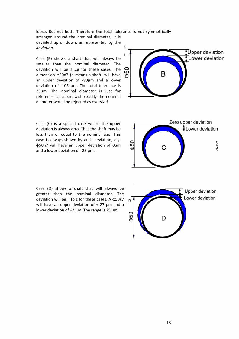
loose. But not both. Therefore the total tolerance is not symmetrically
arranged around the nominal diameter, it is
deviated up or down, as represented by the
deviation.
Case (B) shows a shaft that will always be
smaller than the nominal diameter. The
deviation will be a....g for these cases. The
dimension φ50d7 (d means a shaft) will have
an upper deviation of -80μm and a lower
deviation of -105 μm. The total tolerance is
25μm. The nominal diameter is just for
reference, as a part with exactly the nominal
diameter would be rejected as oversize!
Case (C) is a special case where the upper
deviation is always zero. Thus the shaft may be
less than or equal to the nominal size. This
case is always shown by an h deviation, e.g.
φ50h7 will have an upper deviation of 0μm
and a lower deviation of -25 μm.
Case (D) shows a shaft that will always be
greater than the nominal diameter. The
deviation will be js to z for these cases. A φ50k7
will have an upper deviation of + 27 μm and a
lower deviation of +2 μm. The range is 25 μm.
14
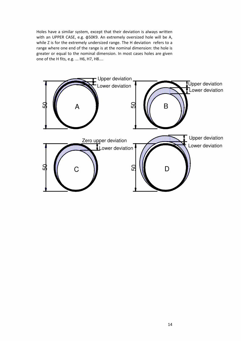
Holes have a similar system, except that their deviation is always written
with an UPPER CASE, e.g. φ50K9. An extremely oversized hole will be A,
while Z is for the extremely undersized range. The H deviation refers to a
range where one end of the range is at the nominal dimension: the hole is
greater or equal to the nominal dimension. In most cases holes are given
one of the H fits, e.g. ... H6, H7, H8....
50
Zero upper deviation
Lower deviation
50
Upper deviation
Lower deviation
50
Upper deviation
Lower deviation
50
Upper deviation
Lower deviation
A B
C D
15
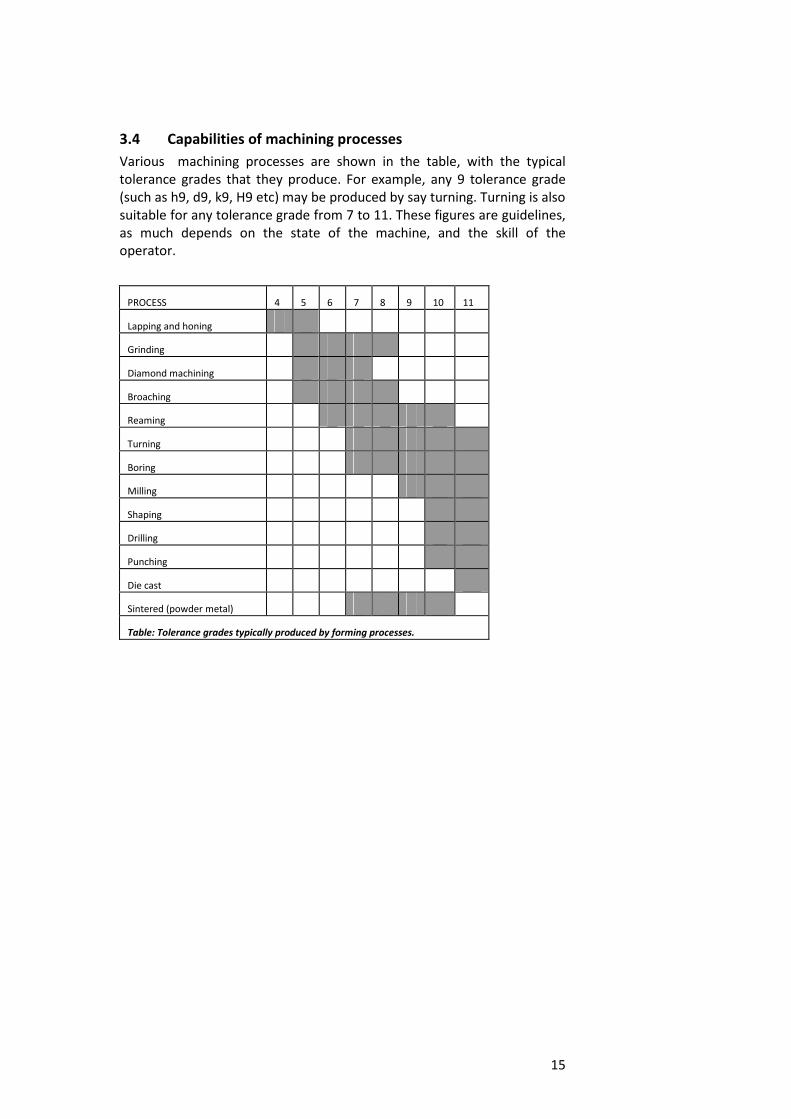
3.4 Capabilities of machining processes
Various machining processes are shown in the table, with the typical
tolerance grades that they produce. For example, any 9 tolerance grade
(such as h9, d9, k9, H9 etc) may be produced by say turning. Turning is also
suitable for any tolerance grade from 7 to 11. These figures are guidelines,
as much depends on the state of the machine, and the skill of the
operator.
PROCESS 4 5 6 7 8 9 10 11
Lapping and honing
Grinding
Diamond machining
Broaching
Reaming
Turning
Boring
Milling
Shaping
Drilling
Punching
Die cast
Sintered (powder metal)
Table: Tolerance grades typically produced by forming processes.
16
3.5 Interface Pressure
Heavy press fits are basically a permanent assembly. The parts are
either forced together axially, or the outer part expanded by heating
(or inner part shrunk by cooling). The tighter the fit, and the larger
the shaft diameter, the greater the torque that can be taken.
Plain press fit
A common requirement is to determine the axial force required to
make/loosen the press fit, and the maximum torque that may be
transmitted.
The following information is required:
R1 inner radius of shaft (zero for solid shaft)
R2 interface radius (or diameter D), eg nominal shaft
diameter at hub or gear blank
R3 outer radius R3. i.e. outer radius of gear hub. For solid
blank use the pitch radius.
ν Poisson's ratio for shaft (inner, i) and hub (outer, o)
E modulus of elasticity for shaft (inner, i) and hub
(outer, o)
Select a fit based on the design intent (see standard
recommendations), e.g. H7/r6
Selected fit:
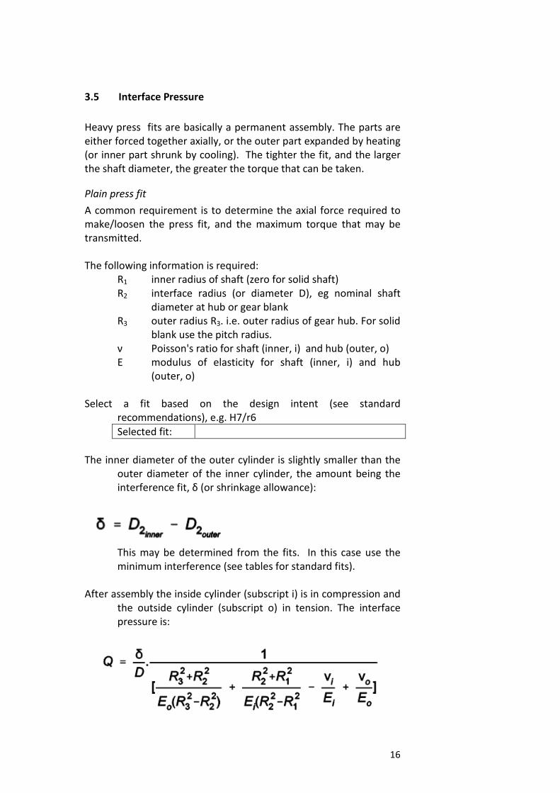
The inner diameter of the outer cylinder is slightly smaller than the
outer diameter of the inner cylinder, the amount being the
interference fit, δ (or shrinkage allowance):
This may be determined from the fits. In this case use the
minimum interference (see tables for standard fits).
After assembly the inside cylinder (subscript i) is in compression and
the outside cylinder (subscript o) in tension. The interface
pressure is:
17
The interface pressure will not usually be the greatest stress in the
assembly, so don’t use this for failure analysis. You will need to do
more work if you want that information too: determine the
circumferential stresses at the inside and outside of the inner and
outer cylinders (four values, inside cylinder negative due to
compression). Radial stresses may also be determined, and an
appropriate failure mechanism used. Consult a reference in
structural mechanics for the details.
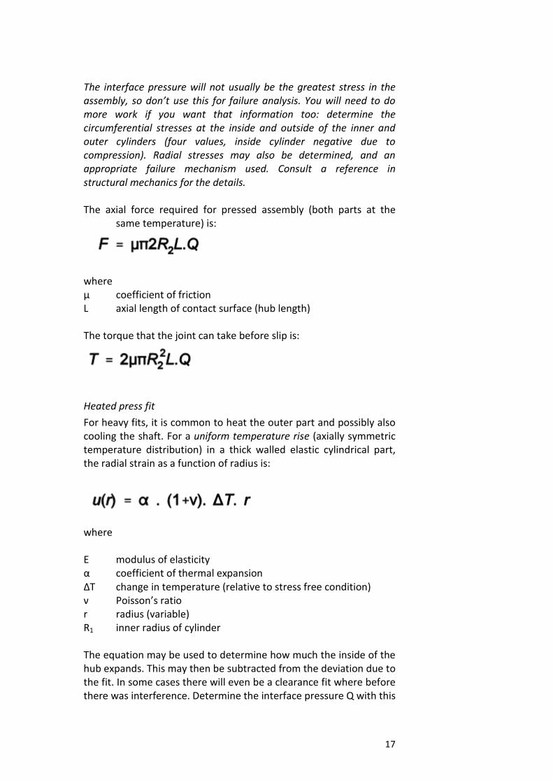
The axial force required for pressed assembly (both parts at the
same temperature) is:
where
μ coefficient of friction
L axial length of contact surface (hub length)
The torque that the joint can take before slip is:
Heated press fit
For heavy fits, it is common to heat the outer part and possibly also
cooling the shaft. For a uniform temperature rise (axially symmetric
temperature distribution) in a thick walled elastic cylindrical part,
the radial strain as a function of radius is:
where
E modulus of elasticity
α coefficient of thermal expansion
ΔT change in temperature (relative to stress free condition)
ν Poisson’s ratio
r radius (variable)
R1 inner radius of cylinder
The equation may be used to determine how much the inside of the
hub expands. This may then be subtracted from the deviation due to
the fit. In some cases there will even be a clearance fit where before
there was interference. Determine the interface pressure Q with this
18
new fit (if it is still interference), and from that get the required axial
assembly force.
Press fit example
A hollow shaft has OD 50 mm and ID 30 mm. It is to carry a solid
gear, with a pitch diameter of 100 mm and a hub length (face width)
of 30 mm. Helix angle 15 deg. The shaft speed is 3000 rpm.
Determine a suitable press fit to transmit 40 kW. Both gear and shaft
of steel. Determine the assembly force required without heating, and
heating the gear by 100oC.
Determine gear loading
Torque required on joint
T = P/ω
= 40 x 103W/(3000 x2π/60 rad/s)
= 127.3 Nm
Axial force
Fa = (2T/d) . Tan(H)
= (2 x 127.3/0.100) x tan(15)
= 682 N
Select fit H7 s6, heavy press fit.
Deviations for Hole D50 H7: +25 -0 μm
Shaft D50 s6: +59 +43 μm
Heaviest fit (Max material condition MMC) 59 -0 = 59 μm
Lightest fit (Least material condition LMC) 43 -25 = 18 μm
It is highly unlikely that the assembly would be in either the
MMC or LMC, rather the deviations would be closer to the
mean. However, for conservative design purposes, we use
the LMC for determining the permissible torque and axial
force, and the MMC for determining the axial assembly force.
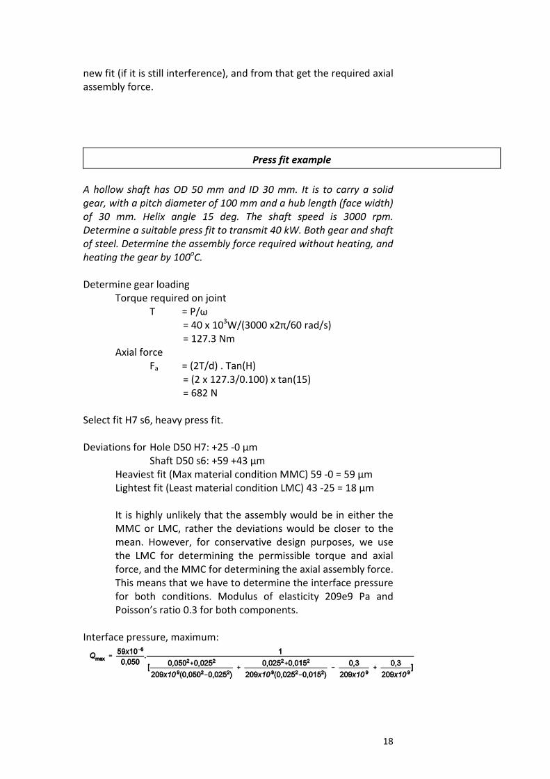
This means that we have to determine the interface pressure
for both conditions. Modulus of elasticity 209e9 Pa and
Poisson’s ratio 0.3 for both components.
Interface pressure, maximum:
19
Qmax = 65.04 MPa
and similarly
Qmin = 19.84 MPa.
Remember to use radii where appropriate.
Coefficient of friction, steel-steel with light oil (see bearings) μ =
0.19.
Then the torque that the joint can take is
Tmax = 2μπR22LQmin
= 2 x 0,19 x π x 0.0252 x 0.030 x 19.84 x 10
-6
= 444 Nm
which is very much greater than the required torque.
The permissible axial force on the joint is
Fallow = 2μπRLQmin
= 2 x 0.19 x π x 0.025 x 0.030 x 19.84 x 10-6
= 17.77 kN,
which is very much greater than the required force.
The maximum assembly force on the joint is
Fassmb = 2μπRLQmax
= 2 x 0.19 x π x 0.025 x 0.030 x 65.04 x 10-6
= 58.2 kN.
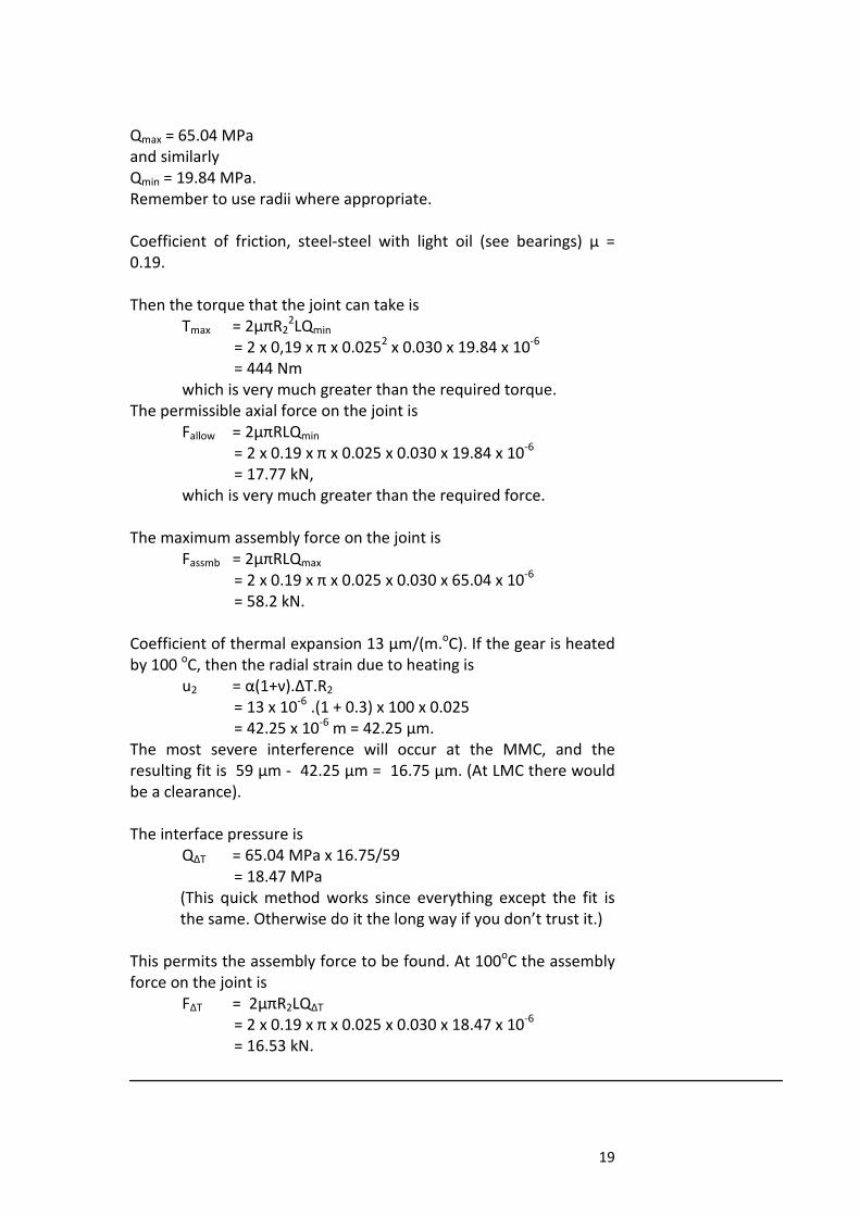
Coefficient of thermal expansion 13 μm/(m.oC). If the gear is heated
by 100 oC, then the radial strain due to heating is
u2 = α(1+ν).ΔT.R2
= 13 x 10-6
.(1 + 0.3) x 100 x 0.025
= 42.25 x 10⁻⁶
m = 42.25 μm.
The most severe interference will occur at the MMC, and the
resulting fit is 59 μm - 42.25 μm = 16.75 μm. (At LMC there would
be a clearance).
The interface pressure is
QΔT = 65.04 MPa x 16.75/59
= 18.47 MPa
(This quick method works since everything except the fit is
the same. Otherwise do it the long way if you don’t trust it.)
This permits the assembly force to be found. At 100oC the assembly
force on the joint is
FΔT = 2μπR2LQΔT
= 2 x 0.19 x π x 0.025 x 0.030 x 18.47 x 10-6
= 16.53 kN.

20
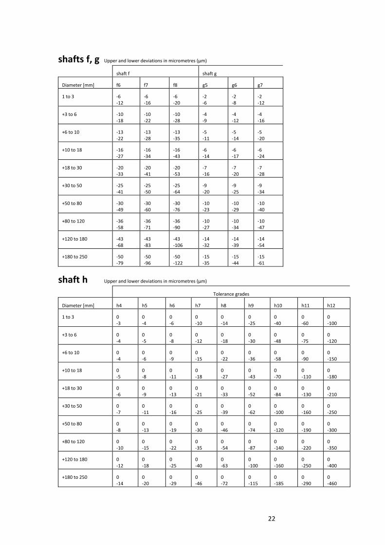
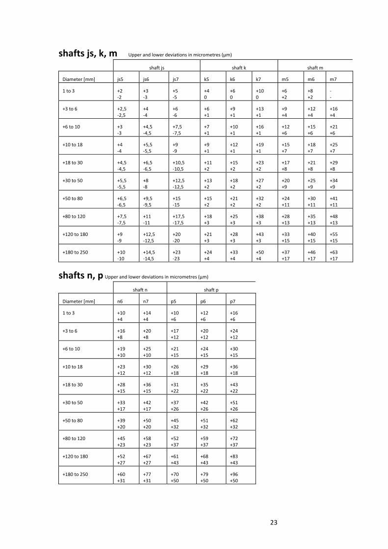
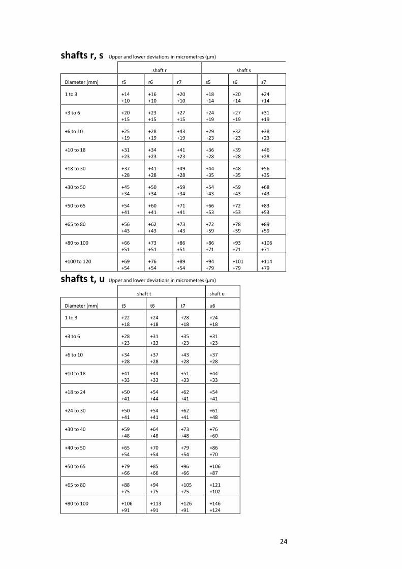
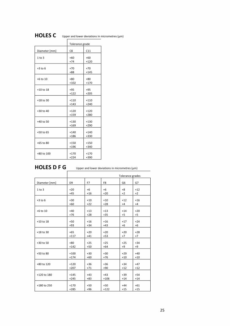
Appendix A: Data for common fits
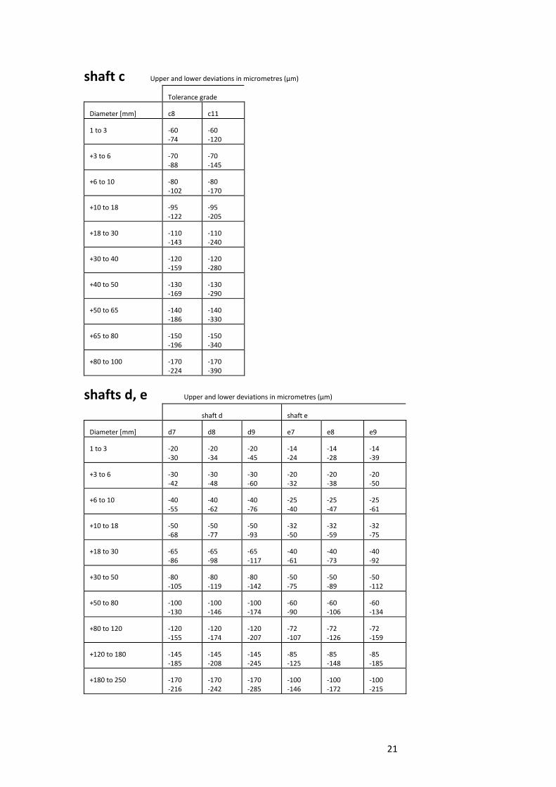
The following tables give the tolerances for various fits. The tolerances
depend on the tolerance grade and the diameter. The tables provide the
tolerances in microns for the dimension, for example a shaft of D50c8 has
tolerances given by the table as -130 and -169. The dimension would then
be 50-0.130 to 50-169.
21
shaft c Upper and lower deviations in micrometres (μm)
Tolerance grade
Diameter [mm] c8 c11
1 to 3 -60
-74
-60
-120
+3 to 6 -70
-88
-70
-145
+6 to 10 -80
-102
-80
-170
+10 to 18 -95
-122
-95
-205
+18 to 30 -110
-143
-110
-240
+30 to 40 -120
-159
-120
-280
+40 to 50 -130
-169
-130
-290
+50 to 65 -140
-186
-140
-330
+65 to 80 -150
-196
-150
-340
+80 to 100 -170
-224
-170
-390
shafts d, e Upper and lower deviations in micrometres (μm)
shaft d shaft e
Diameter [mm] d7 d8 d9 e7 e8 e9
1 to 3 -20
-30
-20
-34
-20
-45
-14
-24
-14
-28
-14
-39
+3 to 6 -30
-42
-30
-48
-30
-60
-20
-32
-20
-38
-20
-50
+6 to 10 -40
-55
-40
-62
-40
-76
-25
-40
-25
-47
-25
-61
+10 to 18 -50
-68
-50
-77
-50
-93
-32
-50
-32
-59
-32
-75
+18 to 30 -65
-86
-65
-98
-65
-117
-40
-61
-40
-73
-40
-92
+30 to 50 -80
-105
-80
-119
-80
-142
-50
-75
-50
-89
-50
-112
+50 to 80 -100
-130
-100
-146
-100
-174
-60
-90
-60
-106
-60
-134
+80 to 120 -120
-155
-120
-174
-120
-207
-72
-107
-72
-126
-72
-159
+120 to 180 -145
-185
-145
-208
-145
-245
-85
-125
-85
-148
-85
-185
+180 to 250 -170
-216
-170
-242
-170
-285
-100
-146
-100
-172
-100
-215
22
shafts f, g Upper and lower deviations in micrometres (μm)
shaft f shaft g
Diameter [mm] f6 f7 f8 g5 g6 g7
1 to 3 -6
-12
-6
-16
-6
-20
-2
-6
-2
-8
-2
-12
+3 to 6 -10
-18
-10
-22
-10
-28
-4
-9
-4
-12
-4
-16
+6 to 10 -13
-22
-13
-28
-13
-35
-5
-11
-5
-14
-5
-20
+10 to 18 -16
-27
-16
-34
-16
-43
-6
-14
-6
-17
-6
-24
+18 to 30 -20
-33
-20
-41
-20
-53
-7
-16
-7
-20
-7
-28
+30 to 50 -25
-41
-25
-50
-25
-64
-9
-20
-9
-25
-9
-34
+50 to 80 -30
-49
-30
-60
-30
-76
-10
-23
-10
-29
-10
-40
+80 to 120 -36
-58
-36
-71
-36
-90
-10
-27
-10
-34
-10
-47
+120 to 180 -43
-68
-43
-83
-43
-106
-14
-32
-14
-39
-14
-54
+180 to 250 -50
-79
-50
-96
-50
-122
-15
-35
-15
-44
-15
-61
shaft h Upper and lower deviations in micrometres (μm)
Tolerance grades
Diameter [mm] h4 h5 h6 h7 h8 h9 h10 h11 h12
1 to 3 0
-3
0
-4
0
-6
0
-10
0
-14
0
-25
0
-40
0
-60
0
-100
+3 to 6 0
-4
0
-5
0
-8
0
-12
0
-18
0
-30
0
-48
0
-75
0
-120
+6 to 10 0
-4
0
-6
0
-9
0
-15
0
-22
0
-36
0
-58
0
-90
0
-150
+10 to 18 0
-5
0
-8
0
-11
0
-18
0
-27
0
-43
0
-70
0
-110
0
-180
+18 to 30 0
-6
0
-9
0
-13
0
-21
0
-33
0
-52
0
-84
0
-130
0
-210
+30 to 50 0
-7
0
-11
0
-16
0
-25
0
-39
0
-62
0
-100
0
-160
0
-250
+50 to 80 0
-8
0
-13
0
-19
0
-30
0
-46
0
-74
0
-120
0
-190
0
-300
+80 to 120 0
-10
0
-15
0
-22
0
-35
0
-54
0
-87
0
-140
0
-220
0
-350
+120 to 180 0
-12
0
-18
0
-25
0
-40
0
-63
0
-100
0
-160
0
-250
0
-400
+180 to 250 0
-14
0
-20
0
-29
0
-46
0
-72
0
-115
0
-185
0
-290
0
-460
23
shafts js, k, m Upper and lower deviations in micrometres (μm)
shaft js shaft k shaft m
Diameter [mm] js5 js6 js7 k5 k6 k7 m5 m6 m7
1 to 3 +2
-2
+3
-3
+5
-5
+4
0
+6
0
+10
0
+6
+2
+8
+2
-
-
+3 to 6 +2,5
-2,5
+4
-4
+6
-6
+6
+1
+9
+1
+13
+1
+9
+4
+12
+4
+16
+4
+6 to 10 +3
-3
+4,5
-4,5
+7,5
-7,5
+7
+1
+10
+1
+16
+1
+12
+6
+15
+6
+21
+6
+10 to 18 +4
-4
+5,5
-5,5
+9
-9
+9
+1
+12
+1
+19
+1
+15
+7
+18
+7
+25
+7
+18 to 30 +4,5
-4,5
+6,5
-6,5
+10,5
-10,5
+11
+2
+15
+2
+23
+2
+17
+8
+21
+8
+29
+8
+30 to 50 +5,5
-5,5
+8
-8
+12,5
-12,5
+13
+2
+18
+2
+27
+2
+20
+9
+25
+9
+34
+9
+50 to 80 +6,5
-6,5
+9,5
-9,5
+15
-15
+15
+2
+21
+2
+32
+2
+24
+11
+30
+11
+41
+11
+80 to 120 +7,5
-7,5
+11
-11
+17,5
-17,5
+18
+3
+25
+3
+38
+3
+28
+13
+35
+13
+48
+13
+120 to 180 +9
-9
+12,5
-12,5
+20
-20
+21
+3
+28
+3
+43
+3
+33
+15
+40
+15
+55
+15
+180 to 250 +10
-10
+14,5
-14,5
+23
-23
+24
+4
+33
+4
+50
+4
+37
+17
+46
+17
+63
+17
shafts n, p Upper and lower deviations in micrometres (μm)
shaft n shaft p
Diameter [mm] n6 n7 p5 p6 p7
1 to 3 +10
+4
+14
+4
+10
+6
+12
+6
+16
+6
+3 to 6 +16
+8
+20
+8
+17
+12
+20
+12
+24
+12
+6 to 10 +19
+10
+25
+10
+21
+15
+24
+15
+30
+15
+10 to 18 +23
+12
+30
+12
+26
+18
+29
+18
+36
+18
+18 to 30 +28
+15
+36
+15
+31
+22
+35
+22
+43
+22
+30 to 50 +33
+17
+42
+17
+37
+26
+42
+26
+51
+26
+50 to 80 +39
+20
+50
+20
+45
+32
+51
+32
+62
+32
+80 to 120 +45
+23
+58
+23
+52
+37
+59
+37
+72
+37
+120 to 180 +52
+27
+67
+27
+61
+43
+68
+43
+83
+43
+180 to 250 +60
+31
+77
+31
+70
+50
+79
+50
+96
+50
24
shafts r, s Upper and lower deviations in micrometres (μm)
shaft r shaft s
Diameter [mm] r5 r6 r7 s5 s6 s7
1 to 3 +14
+10
+16
+10
+20
+10
+18
+14
+20
+14
+24
+14
+3 to 6 +20
+15
+23
+15
+27
+15
+24
+19
+27
+19
+31
+19
+6 to 10 +25
+19
+28
+19
+43
+19
+29
+23
+32
+23
+38
+23
+10 to 18 +31
+23
+34
+23
+41
+23
+36
+28
+39
+28
+46
+28
+18 to 30 +37
+28
+41
+28
+49
+28
+44
+35
+48
+35
+56
+35
+30 to 50 +45
+34
+50
+34
+59
+34
+54
+43
+59
+43
+68
+43
+50 to 65 +54
+41
+60
+41
+71
+41
+66
+53
+72
+53
+83
+53
+65 to 80 +56
+43
+62
+43
+73
+43
+72
+59
+78
+59
+89
+59
+80 to 100 +66
+51
+73
+51
+86
+51
+86
+71
+93
+71
+106
+71
+100 to 120 +69
+54
+76
+54
+89
+54
+94
+79
+101
+79
+114
+79
shafts t, u Upper and lower deviations in micrometres (μm)
shaft t shaft u
Diameter [mm] t5 t6 t7 u6
1 to 3 +22
+18
+24
+18
+28
+18
+24
+18
+3 to 6 +28
+23
+31
+23
+35
+23
+31
+23
+6 to 10 +34
+28
+37
+28
+43
+28
+37
+28
+10 to 18 +41
+33
+44
+33
+51
+33
+44
+33
+18 to 24 +50
+41
+54
+44
+62
+41
+54
+41
+24 to 30 +50
+41
+54
+41
+62
+41
+61
+48
+30 to 40 +59
+48
+64
+48
+73
+48
+76
+60
+40 to 50 +65
+54
+70
+54
+79
+54
+86
+70
+50 to 65 +79
+66
+85
+66
+96
+66
+106
+87
+65 to 80 +88
+75
+94
+75
+105
+75
+121
+102
+80 to 100 +106
+91
+113
+91
+126
+91
+146
+124
25
HOLES C Upper and lower deviations in micrometres (μm)
Tolerance grade
Diameter [mm] C8 C11
1 to 3 +60
+74
+60
+120
+3 to 6 +70
+88
+70
+145
+6 to 10 +80
+102
+80
+170
+10 to 18 +95
+122
+95
+205
+18 to 30 +110
+143
+110
+240
+30 to 40 +120
+159
+120
+280
+40 to 50 +130
+169
+130
+290
+50 to 65 +140
+186
+140
+330
+65 to 80 +150
+196
+150
+340
+80 to 100 +170
+224
+170
+390
HOLES D F G Upper and lower deviations in micrometres (μm)
Tolerance grades
Diameter [mm] D9 F7 F8 G6 G7
1 to 3 +20
+45
+6
+16
+6
+20
+8
+2
+12
+2
+3 to 6 +30
+60
+10
+22
+10
+28
+12
+4
+16
+4
+6 to 10 +40
+76
+13
+28
+13
+35
+14
+5
+20
+5
+10 to 18 +50
+93
+16
+34
+16
+43
+17
+6
+24
+6
+18 to 30 +65
+117
+20
+41
+20
+53
+20
+7
+28
+7
+30 to 50 +80
+142
+25
+50
+25
+64
+25
+9
+34
+9
+50 to 80 +100
+174
+30
+60
+30
+76
+29
+10
+40
+10
+80 to 120 +120
+207
+36
+71
+36
+90
+34
+12
+47
+12
+120 to 180 +145
+245
+43
+83
+43
+106
+39
+14
+54
+14
+180 to 250 +170
+285
+50
+96
+50
+122
+44
+15
+61
+15
26
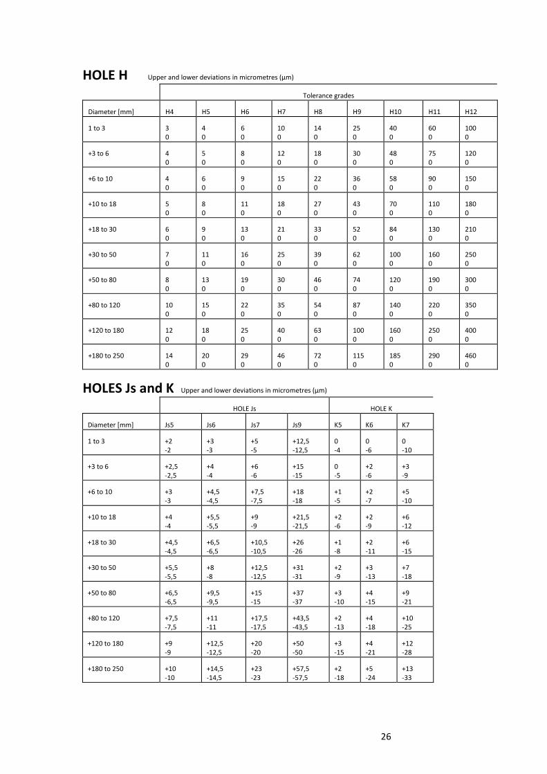
HOLE H Upper and lower deviations in micrometres (μm)
Tolerance grades
Diameter [mm] H4 H5 H6 H7 H8 H9 H10 H11 H12
1 to 3 3
0
4
0
6
0
10
0
14
0
25
0
40
0
60
0
100
0
+3 to 6 4
0
5
0
8
0
12
0
18
0
30
0
48
0
75
0
120
0
+6 to 10 4
0
6
0
9
0
15
0
22
0
36
0
58
0
90
0
150
0
+10 to 18 5
0
8
0
11
0
18
0
27
0
43
0
70
0
110
0
180
0
+18 to 30 6
0
9
0
13
0
21
0
33
0
52
0
84
0
130
0
210
0
+30 to 50 7
0
11
0
16
0
25
0
39
0
62
0
100
0
160
0
250
0
+50 to 80 8
0
13
0
19
0
30
0
46
0
74
0
120
0
190
0
300
0
+80 to 120 10
0
15
0
22
0
35
0
54
0
87
0
140
0
220
0
350
0
+120 to 180 12
0
18
0
25
0
40
0
63
0
100
0
160
0
250
0
400
0
+180 to 250 14
0
20
0
29
0
46
0
72
0
115
0
185
0
290
0
460
0
HOLES Js and K Upper and lower deviations in micrometres (μm)
HOLE Js HOLE K
Diameter [mm] Js5 Js6 Js7 Js9 K5 K6 K7
1 to 3 +2
-2
+3
-3
+5
-5
+12,5
-12,5
0
-4
0
-6
0
-10
+3 to 6 +2,5
-2,5
+4
-4
+6
-6
+15
-15
0
-5
+2
-6
+3
-9
+6 to 10 +3
-3
+4,5
-4,5
+7,5
-7,5
+18
-18
+1
-5
+2
-7
+5
-10
+10 to 18 +4
-4
+5,5
-5,5
+9
-9
+21,5
-21,5
+2
-6
+2
-9
+6
-12
+18 to 30 +4,5
-4,5
+6,5
-6,5
+10,5
-10,5
+26
-26
+1
-8
+2
-11
+6
-15
+30 to 50 +5,5
-5,5
+8
-8
+12,5
-12,5
+31
-31
+2
-9
+3
-13
+7
-18
+50 to 80 +6,5
-6,5
+9,5
-9,5
+15
-15
+37
-37
+3
-10
+4
-15
+9
-21
+80 to 120 +7,5
-7,5
+11
-11
+17,5
-17,5
+43,5
-43,5
+2
-13
+4
-18
+10
-25
+120 to 180 +9
-9
+12,5
-12,5
+20
-20
+50
-50
+3
-15
+4
-21
+12
-28
+180 to 250 +10
-10
+14,5
-14,5
+23
-23
+57,5
-57,5
+2
-18
+5
-24
+13
-33
27
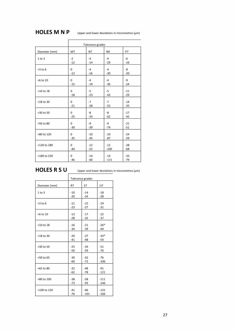
HOLES M N P Upper and lower deviations in micrometres (μm)
Tolerance grades
Diameter [mm] M7 N7 N9 P7
1 to 3 -2
-12
-4
-14
-4
-29
-6
-16
+3 to 6 0
-12
-4
-16
-4
-30
-8
-20
+6 to 10 0
-15
-4
-19
-4
-36
-9
-24
+10 to 18 0
-18
-5
-23
-5
-43
-11
-29
+18 to 30 0
-21
-7
-28
-7
-52
-14
-35
+30 to 50 0
-25
-8
-33
-8
-62
-17
-42
+50 to 80 0
-30
-9
-39
-9
-74
-21
-51
+80 to 120 0
-35
-10
-45
-10
-87
-24
-59
+120 to 180 0
-40
-12
-52
-12
-100
-28
-68
+180 to 250 0
-46
-14
-60
-14
-115
-33
-79
HOLES R S U Upper and lower deviations in micrometres (μm)
Tolerance grades
Diameter [mm] R7 S7 U7
1 to 3 -10
-20
-14
-24
-18
-28
+3 to 6 -11
-23
-15
-27
-19
-31
+6 to 10 -13
-28
-17
-32
-22
-37
+10 to 18 -16
-34
-21
-39
-26*
-44
+18 to 30 -20
-41
-27
-48
-33*
-54
+30 to 50 -25
-50
-34
-59
-51
-76
+50 to 65 -30
-60
-42
-72
-76
-106
+65 to 80 -32
-62
-48
-78
-91
-121
+80 to 100 -38
-73
-58
-93
-111
-146
+100 to 120 -41
-76
-66
-101
-131
-166
28
4 Geometric tolerances
4.1 Introduction
The geometry produced by typical machining processes may be acceptable
for many purposes. However where greater accuracy of flatness,
concentricity or other form is required than conventional fabrication will
provide, then geometric tolerances are used by the designer to
communicate the requirements.
This section will provide an overview, and fuller detail may be found in
national standards. Two main standards are ISO 1101 (Europe) and ANSI
Y14.5 (USA). The ISO standard has been adopted in various other countries
under other names (e.g. BS308 Part 3, SABS 0111 part 2, AS1100 part 101).
Although there are small differences, the principles are the same.
Geometric tolerances are a special type of tolerance that is used to control
the accuracy of the surface shape of a part. The tolerances are used in
addition to the plain linear tolerances described above. Geometric
tolerances are tolerances that are applied to characteristics of:
C straightness
C flatness
C circularity
C cylindricity
C line profile
C surface profile
C parallelism
C perpendicularity
C angle
C position
C concentricity
C symmetry
C circular run out
C total run out
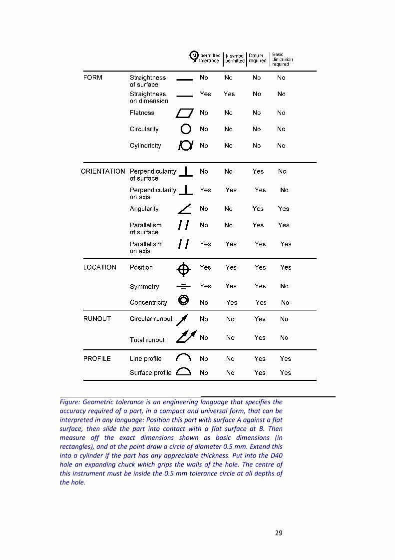
Each of these characteristics has its own symbol, and this is used on the
drawing, together with the tolerance that the designer permits. A
rectangular control frame is used around the geometric tolerance.
29
Figure: Geometric tolerance is an engineering language that specifies the
accuracy required of a part, in a compact and universal form, that can be
interpreted in any language: Position this part with surface A against a flat
surface, then slide the part into contact with a flat surface at B. Then
measure off the exact dimensions shown as basic dimensions (in
rectangles), and at the point draw a circle of diameter 0.5 mm. Extend this
into a cylinder if the part has any appreciable thickness. Put into the D40
hole an expanding chuck which grips the walls of the hole. The centre of
this instrument must be inside the 0.5 mm tolerance circle at all depths of
the hole.
30
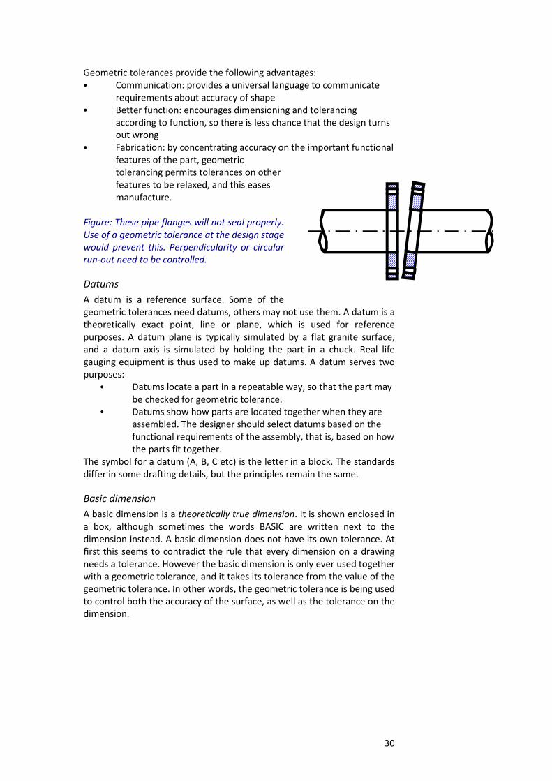
Geometric tolerances provide the following advantages:
C Communication: provides a universal language to communicate
requirements about accuracy of shape
C Better function: encourages dimensioning and tolerancing
according to function, so there is less chance that the design turns
out wrong
C Fabrication: by concentrating accuracy on the important functional
features of the part, geometric
tolerancing permits tolerances on other
features to be relaxed, and this eases
manufacture.
Figure: These pipe flanges will not seal properly.
Use of a geometric tolerance at the design stage
would prevent this. Perpendicularity or circular
run-out need to be controlled.
Datums
A datum is a reference surface. Some of the
geometric tolerances need datums, others may not use them. A datum is a
theoretically exact point, line or plane, which is used for reference
purposes. A datum plane is typically simulated by a flat granite surface,
and a datum axis is simulated by holding the part in a chuck. Real life
gauging equipment is thus used to make up datums. A datum serves two
purposes:
C Datums locate a part in a repeatable way, so that the part may
be checked for geometric tolerance.
C Datums show how parts are located together when they are
assembled. The designer should select datums based on the
functional requirements of the assembly, that is, based on how
the parts fit together.
The symbol for a datum (A, B, C etc) is the letter in a block. The standards
differ in some drafting details, but the principles remain the same.
Basic dimension
A basic dimension is a theoretically true dimension. It is shown enclosed in
a box, although sometimes the words BASIC are written next to the
dimension instead. A basic dimension does not have its own tolerance. At
first this seems to contradict the rule that every dimension on a drawing
needs a tolerance. However the basic dimension is only ever used together
with a geometric tolerance, and it takes its tolerance from the value of the
geometric tolerance. In other words, the geometric tolerance is being used
to control both the accuracy of the surface, as well as the tolerance on the
dimension.
31
Where is the geometric tolerance applied?
The geometric tolerance is generally applied directly to a surface, with an
arrow. Some geometric tolerances can instead be applied underneath a
diameter. This means that the tolerance applies to the centre line of that
hole, and therefore indirectly to the surface concerned. When a geometric
tolerance is applied underneath a dimension, then it is still permissible for
that dimension to have its own tolerance.
How big to make the geometric tolerance?
The value will depend on the function required. Determine the virtual
condition of the parts (defined later), and see if they fit together. This will
help you set the geometric tolerances. Remember that the geometric
tolerances must generally be smaller than the linear (or plain) tolerances,
in order to have any effect. The values given in the examples here are
deliberately large.
Maximum material condition MMC
The MMC is the extreme tolerance state in which the part has maximum
material (maximum mass). There are two benefits of MMC, first that a
bonus tolerance is available to the fabricator, and second that fixed gauges
may be used. This is really useful in production, and we return to this
topic later.
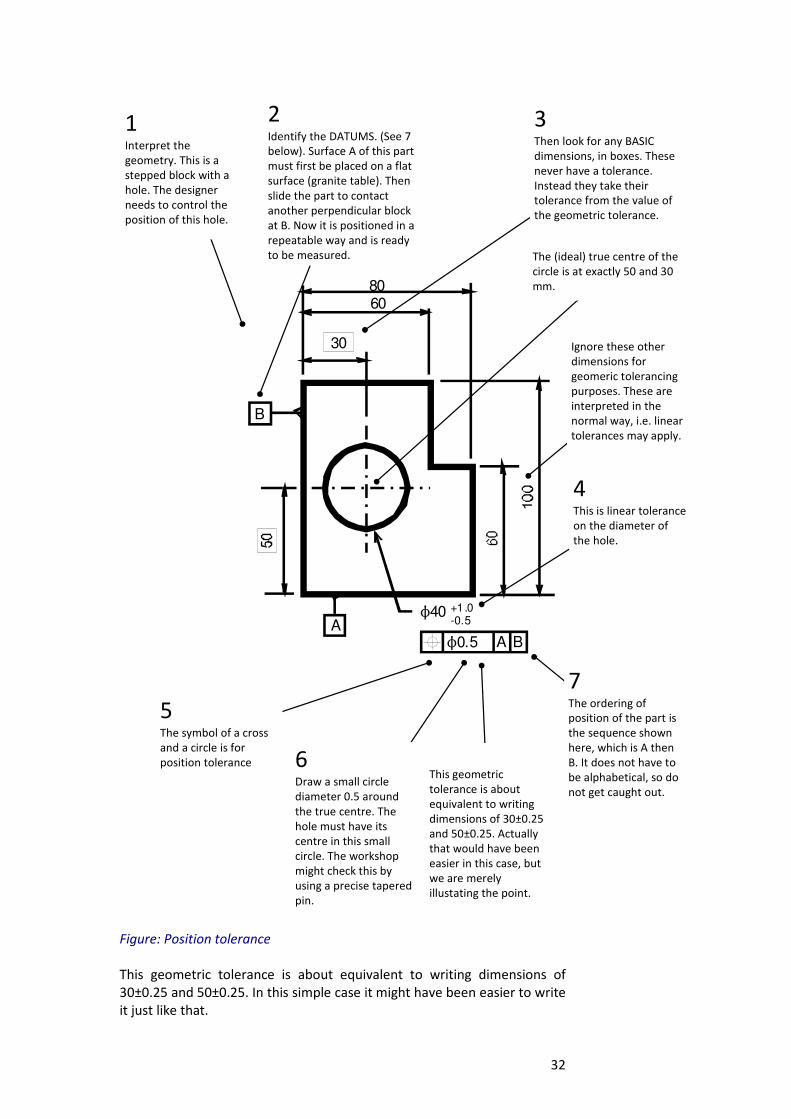
Typical application
The figure shows an example of a geometric tolerance for Position.
Underneath the N40 is the geometric tolerance in its frame. The tolerance
reads like this: the centre of the N40 hole must be positioned within circle
of diameter 0.5 of the true centre of the circle. The symbol of a cross and a
circle is for position. The true centre of the circle is at exactly 50 and 30
mm. The datum planes are A and B, and this means that when checking
this part, surface A must first be placed against a “perfectly” flat surface,
and then surface B brought against another such surface at right angles to
A. The measuring surfaces are usually granite blocks, granite being used
since it distorts very little with change in temperature.
32
N40
30
8060
N0.5 A BA
B
+1.0-0.5
2Identify the DATUMS. (See 7
below). Surface A of this part
must first be placed on a flat
surface (granite table). Then
slide the part to contact
another perpendicular block
at B. Now it is positioned in a
repeatable way and is ready
to be measured.
3Then look for any BASIC
dimensions, in boxes. These
never have a tolerance.
Instead they take their
tolerance from the value of
the geometric tolerance.
Ignore these other
dimensions for
geomeric tolerancing
purposes. These are
interpreted in the
normal way, i.e. linear
tolerances may apply.
1Interpret the
geometry. This is a
stepped block with a
hole. The designer
needs to control the
position of this hole.
5The symbol of a cross
and a circle is for
position tolerance
The (ideal) true centre of the
circle is at exactly 50 and 30
mm.
This geometric
tolerance is about
equivalent to writing
dimensions of 30±0.25
and 50±0.25. Actually
that would have been
easier in this case, but
we are merely
illustating the point.
6Draw a small circle
diameter 0.5 around
the true centre. The
hole must have its
centre in this small
circle. The workshop
might check this by
using a precise tapered
pin.
7The ordering of
position of the part is
the sequence shown
here, which is A then
B. It does not have to
be alphabetical, so do
not get caught out.
4This is linear tolerance
on the diameter of
the hole.
Figure: Position tolerance
This geometric tolerance is about equivalent to writing dimensions of
30±0.25 and 50±0.25. In this simple case it might have been easier to write
it just like that.
33
A key needsto fit into aslot...
...and theslot would bedimensionedlike this.
This wouldbe the wrongway
Applying geometric tolerances
The first step that the designer needs to take is to decide whether or not
geometric tolerances are necessary. This decision is based on the required
function of the part and especially the assembly of the parts. The function
is known best to the designer, so this is where the responsibility of the
decision lies. It is poor design to apply geometric tolerances to every
dimension in sight: rather concentrate on those features that affect the
function.
Features that affect function are
G Surfaces that touch other parts. As soon as parts are required to fit
together, then the accuracy of the surfaces will affect the
alignment of the assembly. The designer should check each surface
that touches another surface, and determine how much
misalignment can be tolerated. The example shows how
misalignment of pipe flanges can impair function. Use of geometric
tolerances at the design stage is the best way to ensure that the
part can fulfil the intended function. Just how big a tolerance to
allow is up to the discretion of the designer, since it depends on
function.
G In any design there will be surfaces that are only in contact with
the air: no other part touches them. These surfaces do not
generally need to be highly accurate in geometry. Therefore such
surfaces would not generally need geometric tolerances. Optically
active surfaces (e.g. telescope
mirrors) are an exception here.
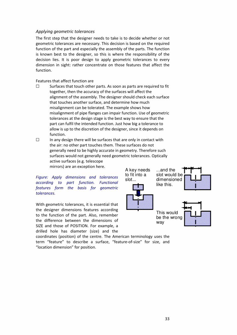
Figure: Apply dimensions and tolerances
according to part function. Functional
features form the basis for geometric
tolerances.
With geometric tolerances, it is essential that
the designer dimensions features according
to the function of the part. Also, remember
the difference between the dimensions of
SIZE and those of POSITION. For example, a
drilled hole has diameter (size) and the
coordinates (position) of the centre. The American terminology uses the
term “feature” to describe a surface, “feature-of-size” for size, and
“location dimension” for position.
34
4.2 Runout controls
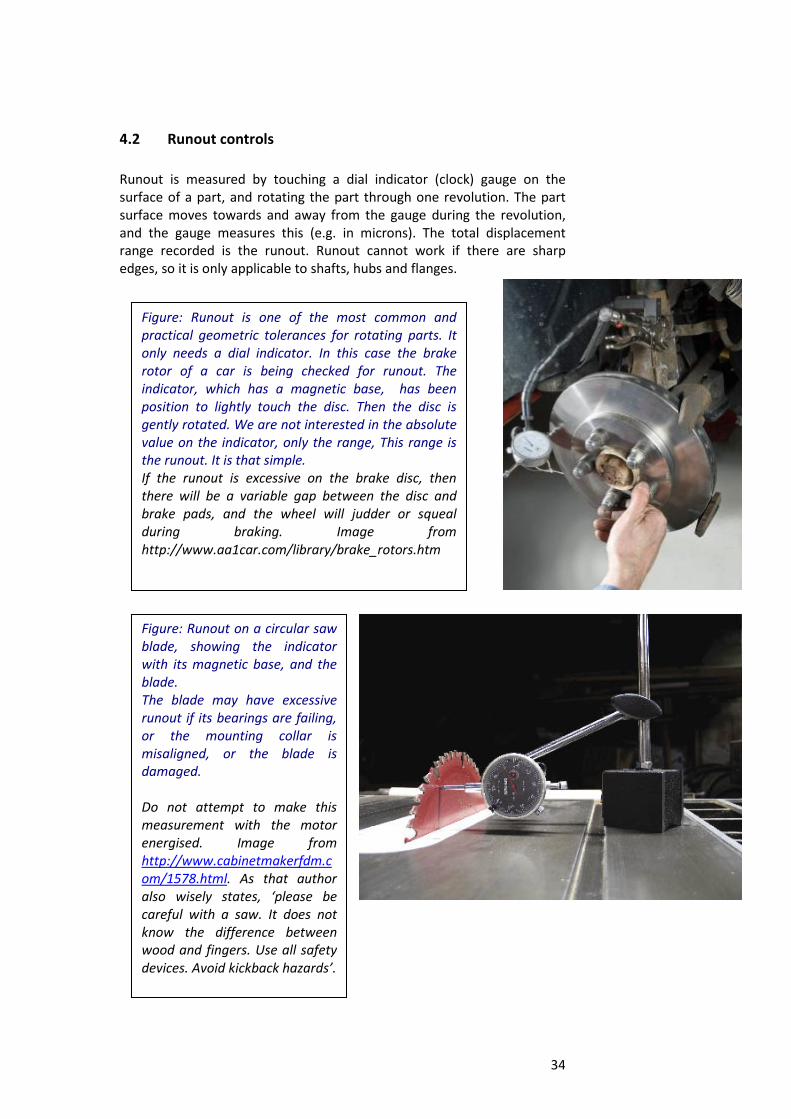
Runout is measured by touching a dial indicator (clock) gauge on the
surface of a part, and rotating the part through one revolution. The part
surface moves towards and away from the gauge during the revolution,
and the gauge measures this (e.g. in microns). The total displacement
range recorded is the runout. Runout cannot work if there are sharp
edges, so it is only applicable to shafts, hubs and flanges.
Figure: Runout is one of the most common and
practical geometric tolerances for rotating parts. It
only needs a dial indicator. In this case the brake
rotor of a car is being checked for runout. The
indicator, which has a magnetic base, has been
position to lightly touch the disc. Then the disc is
gently rotated. We are not interested in the absolute
value on the indicator, only the range, This range is
the runout. It is that simple.
If the runout is excessive on the brake disc, then
there will be a variable gap between the disc and
brake pads, and the wheel will judder or squeal
during braking. Image from
http://www.aa1car.com/library/brake_rotors.htm
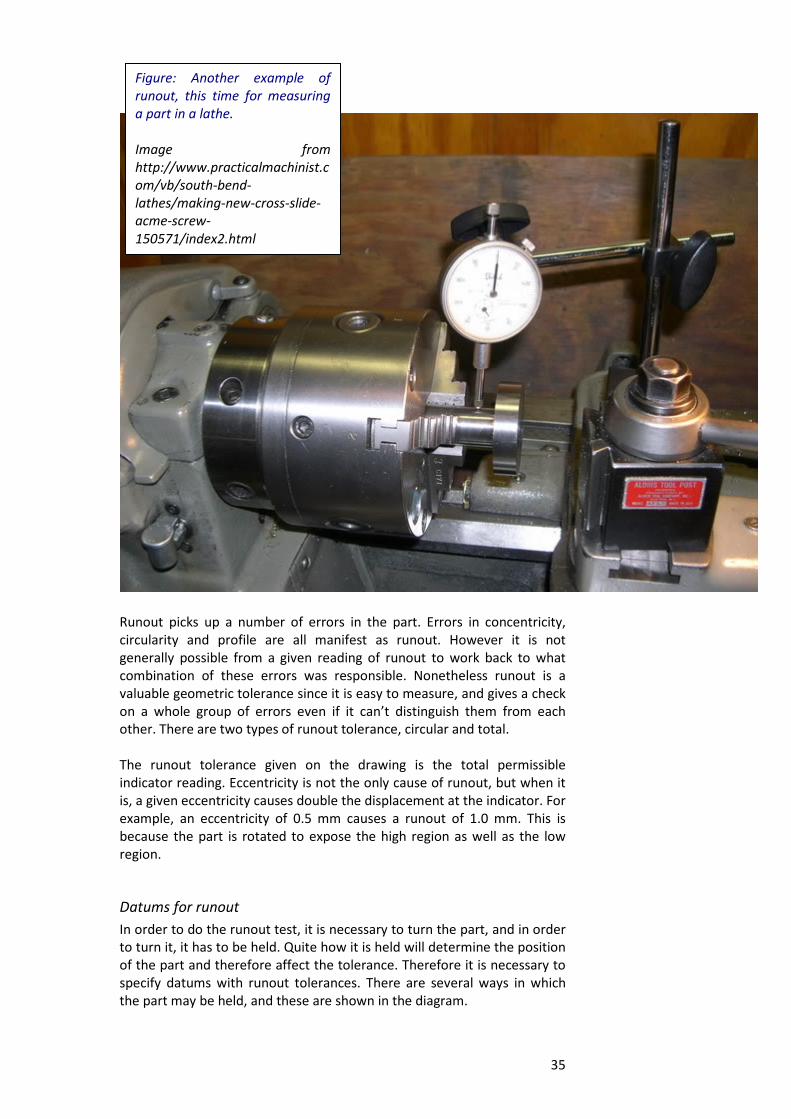
Figure: Runout on a circular saw
blade, showing the indicator
with its magnetic base, and the
blade.
The blade may have excessive
runout if its bearings are failing,
or the mounting collar is
misaligned, or the blade is
damaged.
Do not attempt to make this
measurement with the motor
energised. Image from
http://www.cabinetmakerfdm.c
om/1578.html. As that author
also wisely states, ‘please be
careful with a saw. It does not
know the difference between
wood and fingers. Use all safety
devices. Avoid kickback hazards’.
35
Runout picks up a number of errors in the part. Errors in concentricity,
circularity and profile are all manifest as runout. However it is not
generally possible from a given reading of runout to work back to what
combination of these errors was responsible. Nonetheless runout is a
valuable geometric tolerance since it is easy to measure, and gives a check
on a whole group of errors even if it can’t distinguish them from each
other. There are two types of runout tolerance, circular and total.
The runout tolerance given on the drawing is the total permissible
indicator reading. Eccentricity is not the only cause of runout, but when it
is, a given eccentricity causes double the displacement at the indicator. For
example, an eccentricity of 0.5 mm causes a runout of 1.0 mm. This is
because the part is rotated to expose the high region as well as the low
region.
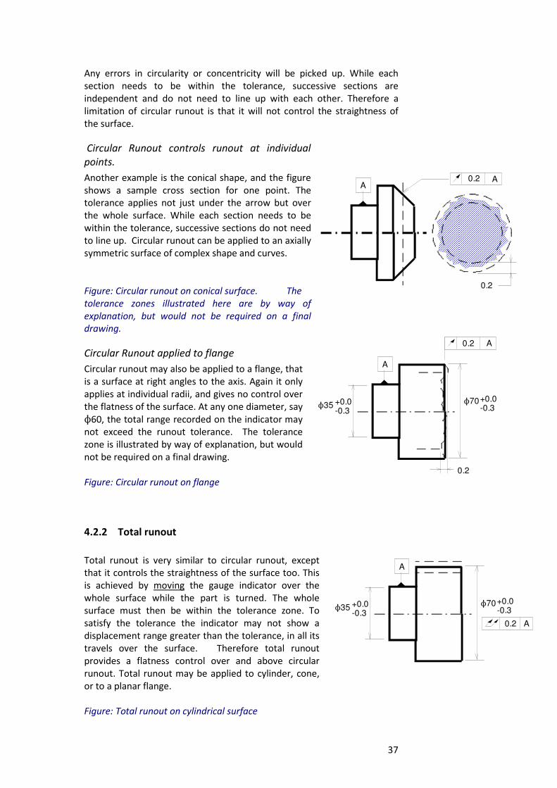
Datums for runout
In order to do the runout test, it is necessary to turn the part, and in order
to turn it, it has to be held. Quite how it is held will determine the position
of the part and therefore affect the tolerance. Therefore it is necessary to
specify datums with runout tolerances. There are several ways in which
the part may be held, and these are shown in the diagram.
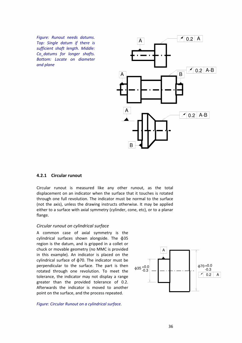
Figure: Another example of
runout, this time for measuring
a part in a lathe.
Image from
http://www.practicalmachinist.c
om/vb/south-bend-
lathes/making-new-cross-slide-
acme-screw-
150571/index2.html
36
0.2 A-BB
A
A
A
B
0.2 A-B
0.2 A
Figure: Runout needs datums.
Top: Single datum if there is
sufficient shaft length. Middle:
Co_datums for longer shafts.
Bottom: Locate on diameter
and plane
4.2.1 Circular runout
Circular runout is measured like any other runout, as the total
displacement on an indicator when the surface that it touches is rotated
through one full revolution. The indicator must be normal to the surface
(not the axis), unless the drawing instructs otherwise. It may be applied
either to a surface with axial symmetry (cylinder, cone, etc), or to a planar
flange.
Circular runout on cylindrical surface
A common case of axial symmetry is the
cylindrical surfaces shown alongside. The N35
region is the datum, and is gripped in a collet or
chuck or movable geometry (no MMC is provided
in this example). An indicator is placed on the
cylindrical surface of N70. The indicator must be
perpendicular to the surface. The part is then
rotated through one revolution. To meet the
tolerance, the indicator may not display a range
greater than the provided tolerance of 0.2.
Afterwards the indicator is moved to another
point on the surface, and the process repeated.
Figure: Circular Runout on a cylindrical surface.
A
0.2 A
N70+0.0-0.3N35 +0.0
-0.3
37
A0.2 A
0.2
A
0.2 A
N70+0.0-0.3N35 +0.0
-0.3
0.2
A
N70+0.0-0.3N35 +0.0
-0.3
0.2 A
Any errors in circularity or concentricity will be picked up. While each
section needs to be within the tolerance, successive sections are
independent and do not need to line up with each other. Therefore a
limitation of circular runout is that it will not control the straightness of
the surface.
Circular Runout controls runout at individual
points.
Another example is the conical shape, and the figure
shows a sample cross section for one point. The
tolerance applies not just under the arrow but over
the whole surface. While each section needs to be
within the tolerance, successive sections do not need
to line up. Circular runout can be applied to an axially
symmetric surface of complex shape and curves.
Figure: Circular runout on conical surface. The
tolerance zones illustrated here are by way of
explanation, but would not be required on a final
drawing.
Circular Runout applied to flange
Circular runout may also be applied to a flange, that
is a surface at right angles to the axis. Again it only
applies at individual radii, and gives no control over
the flatness of the surface. At any one diameter, say
N60, the total range recorded on the indicator may
not exceed the runout tolerance. The tolerance
zone is illustrated by way of explanation, but would
not be required on a final drawing.
Figure: Circular runout on flange
4.2.2 Total runout
Total runout is very similar to circular runout, except
that it controls the straightness of the surface too. This
is achieved by moving the gauge indicator over the
whole surface while the part is turned. The whole
surface must then be within the tolerance zone. To
satisfy the tolerance the indicator may not show a
displacement range greater than the tolerance, in all its
travels over the surface. Therefore total runout
provides a flatness control over and above circular
runout. Total runout may be applied to cylinder, cone,
or to a planar flange.
Figure: Total runout on cylindrical surface
38
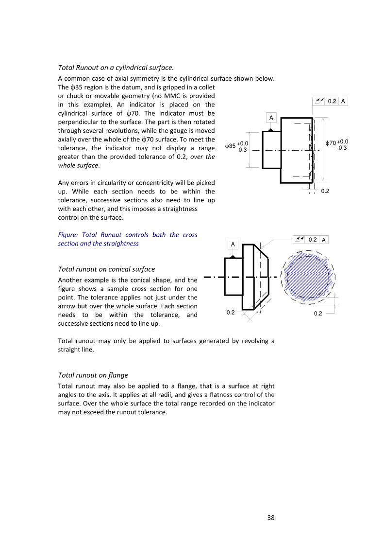
Total Runout on a cylindrical surface.
A common case of axial symmetry is the cylindrical surface shown below.
The N35 region is the datum, and is gripped in a collet
or chuck or movable geometry (no MMC is provided
in this example). An indicator is placed on the
cylindrical surface of N70. The indicator must be
perpendicular to the surface. The part is then rotated
through several revolutions, while the gauge is moved
axially over the whole of the N70 surface. To meet the
tolerance, the indicator may not display a range
greater than the provided tolerance of 0.2, over the
whole surface.
Any errors in circularity or concentricity will be picked
up. While each section needs to be within the
tolerance, successive sections also need to line up
with each other, and this imposes a straightness
control on the surface.
Figure: Total Runout controls both the cross
section and the straightness
Total runout on conical surface
Another example is the conical shape, and the
figure shows a sample cross section for one
point. The tolerance applies not just under the
arrow but over the whole surface. Each section
needs to be within the tolerance, and
successive sections need to line up.
Total runout may only be applied to surfaces generated by revolving a
straight line.
Total runout on flange
Total runout may also be applied to a flange, that is a surface at right
angles to the axis. It applies at all radii, and gives a flatness control of the
surface. Over the whole surface the total range recorded on the indicator
may not exceed the runout tolerance.
A0.2 A
0.20.2
A
N70+0.0-0.3N35 +0.0
-0.3
0.2
0.2 A
39
4.3 Geometric tolerances of form
The geometric tolerances that describe the form (shape) of a surface are
flatness, straightness, circularity, and cylindricity. These geometric
tolerances apply to single features, and they never use datums.
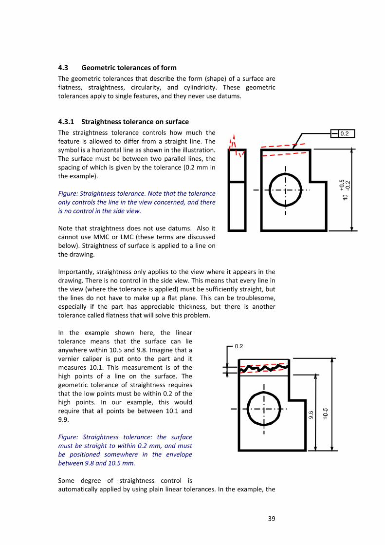
4.3.1 Straightness tolerance on surface
The straightness tolerance controls how much the
feature is allowed to differ from a straight line. The
symbol is a horizontal line as shown in the illustration.
The surface must be between two parallel lines, the
spacing of which is given by the tolerance (0.2 mm in
the example).
Figure: Straightness tolerance. Note that the tolerance
only controls the line in the view concerned, and there
is no control in the side view.
Note that straightness does not use datums. Also it
cannot use MMC or LMC (these terms are discussed
below). Straightness of surface is applied to a line on
the drawing.
Importantly, straightness only applies to the view where it appears in the
drawing. There is no control in the side view. This means that every line in
the view (where the tolerance is applied) must be sufficiently straight, but
the lines do not have to make up a flat plane. This can be troublesome,
especially if the part has appreciable thickness, but there is another
tolerance called flatness that will solve this problem.
In the example shown here, the linear
tolerance means that the surface can lie
anywhere within 10.5 and 9.8. Imagine that a
vernier caliper is put onto the part and it
measures 10.1. This measurement is of the
high points of a line on the surface. The
geometric tolerance of straightness requires
that the low points must be within 0.2 of the
high points. In our example, this would
require that all points be between 10.1 and
9.9.
Figure: Straightness tolerance: the surface
must be straight to within 0.2 mm, and must
be positioned somewhere in the envelope
between 9.8 and 10.5 mm.
Some degree of straightness control is
automatically applied by using plain linear tolerances. In the example, the
0.2
0.2
40
surface would have to be flat within 9.8 to 10.5 mm anyway, because
these are the linear tolerances. When this control is insufficient, then add
a straightness tolerance. This is what has been done in the example. The
geometric tolerance is always smaller than the linear tolerance, so that the
geometric tolerance zone floats within the linear tolerance zone.
Straightness does not affect virtual condition, since the tolerance is
measured into the material.
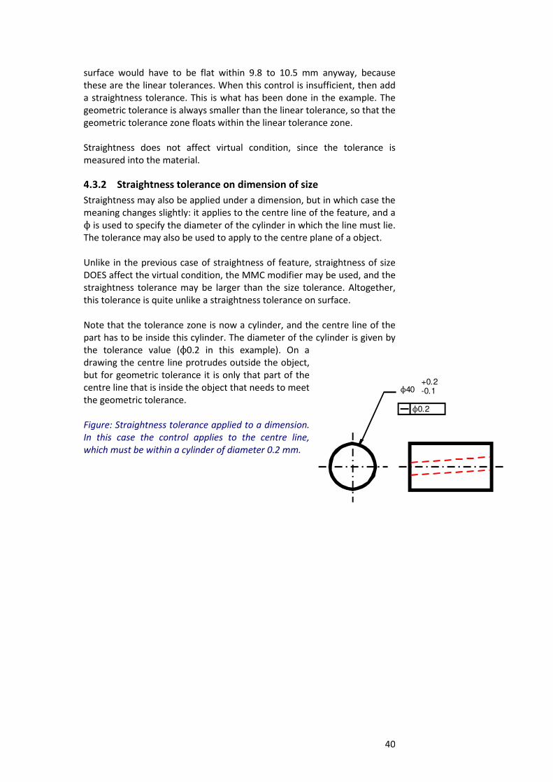
4.3.2 Straightness tolerance on dimension of size
Straightness may also be applied under a dimension, but in which case the
meaning changes slightly: it applies to the centre line of the feature, and a
N is used to specify the diameter of the cylinder in which the line must lie.
The tolerance may also be used to apply to the centre plane of a object.
Unlike in the previous case of straightness of feature, straightness of size
DOES affect the virtual condition, the MMC modifier may be used, and the
straightness tolerance may be larger than the size tolerance. Altogether,
this tolerance is quite unlike a straightness tolerance on surface.
Note that the tolerance zone is now a cylinder, and the centre line of the
part has to be inside this cylinder. The diameter of the cylinder is given by
the tolerance value (N0.2 in this example). On a
drawing the centre line protrudes outside the object,
but for geometric tolerance it is only that part of the
centre line that is inside the object that needs to meet
the geometric tolerance.
Figure: Straightness tolerance applied to a dimension.
In this case the control applies to the centre line,
which must be within a cylinder of diameter 0.2 mm.
N0.2
N40+0.2-0.1
41
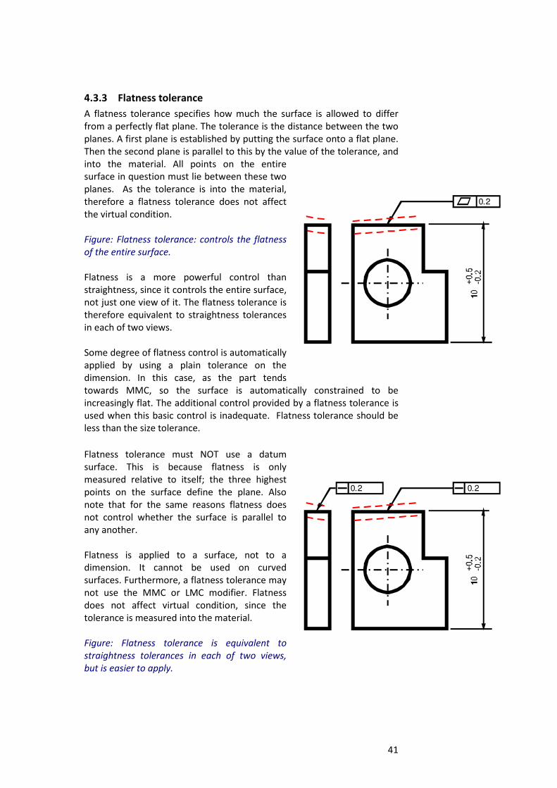
4.3.3 Flatness tolerance
A flatness tolerance specifies how much the surface is allowed to differ
from a perfectly flat plane. The tolerance is the distance between the two
planes. A first plane is established by putting the surface onto a flat plane.
Then the second plane is parallel to this by the value of the tolerance, and
into the material. All points on the entire
surface in question must lie between these two
planes. As the tolerance is into the material,
therefore a flatness tolerance does not affect
the virtual condition.
Figure: Flatness tolerance: controls the flatness
of the entire surface.
Flatness is a more powerful control than
straightness, since it controls the entire surface,
not just one view of it. The flatness tolerance is
therefore equivalent to straightness tolerances
in each of two views.
Some degree of flatness control is automatically
applied by using a plain tolerance on the
dimension. In this case, as the part tends
towards MMC, so the surface is automatically constrained to be
increasingly flat. The additional control provided by a flatness tolerance is
used when this basic control is inadequate. Flatness tolerance should be
less than the size tolerance.
Flatness tolerance must NOT use a datum
surface. This is because flatness is only
measured relative to itself; the three highest
points on the surface define the plane. Also
note that for the same reasons flatness does
not control whether the surface is parallel to
any another.
Flatness is applied to a surface, not to a
dimension. It cannot be used on curved
surfaces. Furthermore, a flatness tolerance may
not use the MMC or LMC modifier. Flatness
does not affect virtual condition, since the
tolerance is measured into the material.
Figure: Flatness tolerance is equivalent to
straightness tolerances in each of two views,
but is easier to apply.
0.2
0.2 0.2
42
0.2
0.2
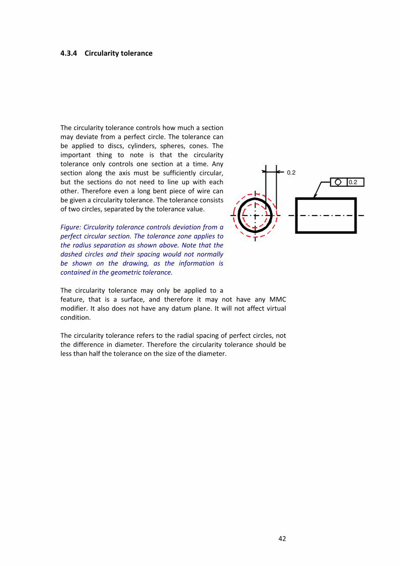
4.3.4 Circularity tolerance
The circularity tolerance controls how much a section
may deviate from a perfect circle. The tolerance can
be applied to discs, cylinders, spheres, cones. The
important thing to note is that the circularity
tolerance only controls one section at a time. Any
section along the axis must be sufficiently circular,
but the sections do not need to line up with each
other. Therefore even a long bent piece of wire can
be given a circularity tolerance. The tolerance consists
of two circles, separated by the tolerance value.
Figure: Circularity tolerance controls deviation from a
perfect circular section. The tolerance zone applies to
the radius separation as shown above. Note that the
dashed circles and their spacing would not normally
be shown on the drawing, as the information is
contained in the geometric tolerance.
The circularity tolerance may only be applied to a
feature, that is a surface, and therefore it may not have any MMC
modifier. It also does not have any datum plane. It will not affect virtual
condition.
The circularity tolerance refers to the radial spacing of perfect circles, not
the difference in diameter. Therefore the circularity tolerance should be
less than half the tolerance on the size of the diameter.
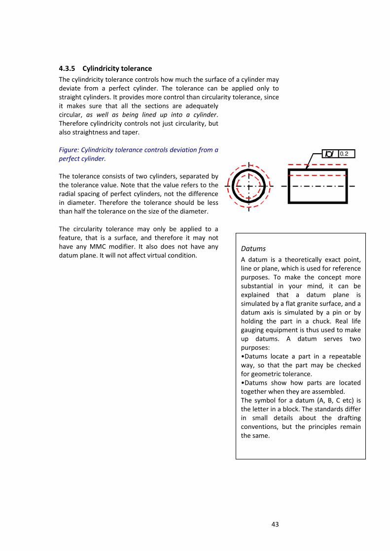
43
4.3.5 Cylindricity tolerance
The cylindricity tolerance controls how much the surface of a cylinder may
deviate from a perfect cylinder. The tolerance can be applied only to
straight cylinders. It provides more control than circularity tolerance, since
it makes sure that all the sections are adequately
circular, as well as being lined up into a cylinder.
Therefore cylindricity controls not just circularity, but
also straightness and taper.
Figure: Cylindricity tolerance controls deviation from a
perfect cylinder.
The tolerance consists of two cylinders, separated by
the tolerance value. Note that the value refers to the
radial spacing of perfect cylinders, not the difference
in diameter. Therefore the tolerance should be less
than half the tolerance on the size of the diameter.
The circularity tolerance may only be applied to a
feature, that is a surface, and therefore it may not
have any MMC modifier. It also does not have any
datum plane. It will not affect virtual condition.
0.2
Datums
A datum is a theoretically exact point,
line or plane, which is used for reference
purposes. To make the concept more
substantial in your mind, it can be
explained that a datum plane is
simulated by a flat granite surface, and a
datum axis is simulated by a pin or by
holding the part in a chuck. Real life
gauging equipment is thus used to make
up datums. A datum serves two
purposes:
•Datums locate a part in a repeatable
way, so that the part may be checked
for geometric tolerance.
•Datums show how parts are located
together when they are assembled.
The symbol for a datum (A, B, C etc) is
the letter in a block. The standards differ
in small details about the drafting
conventions, but the principles remain
the same.
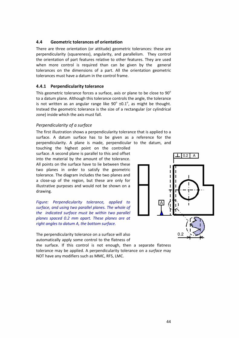
44
4.4 Geometric tolerances of orientation
There are three orientation (or attitude) geometric tolerances: these are
perpendicularity (squareness), angularity, and parallelism. They control
the orientation of part features relative to other features. They are used
when more control is required than can be given by the general
tolerances on the dimensions of a part. All the orientation geometric
tolerances must have a datum in the control frame.
4.4.1 Perpendicularity tolerance
This geometric tolerance forces a surface, axis or plane to be close to 90o
to a datum plane. Although this tolerance controls the angle, the tolerance
is not written as an angular range like 90o ±0.1
o, as might be thought.
Instead the geometric tolerance is the size of a rectangular (or cylindrical
zone) inside which the axis must fall.
Perpendicularity of a surface
The first illustration shows a perpendicularity tolerance that is applied to a
surface. A datum surface has to be given as a reference for the
perpendicularity. A plane is made, perpendicular to the datum, and
touching the highest point on the controlled
surface. A second plane is parallel to this and offset
into the material by the amount of the tolerance.
All points on the surface have to lie between these
two planes in order to satisfy the geometric
tolerance. The diagram includes the two planes and
a close-up of the region, but these are only for
illustrative purposes and would not be shown on a
drawing.
Figure: Perpendicularity tolerance, applied to
surface, and using two parallel planes. The whole of
the indicated surface must be within two parallel
planes spaced 0.2 mm apart. These planes are at
right angles to datum A, the bottom surface.
The perpendicularity tolerance on a surface will also
automatically apply some control to the flatness of
the surface. If this control is not enough, then a separate flatness
tolerance may be applied. A perpendicularity tolerance on a surface may
NOT have any modifiers such as MMC, RFS, LMC.
A0.2
A
0.2
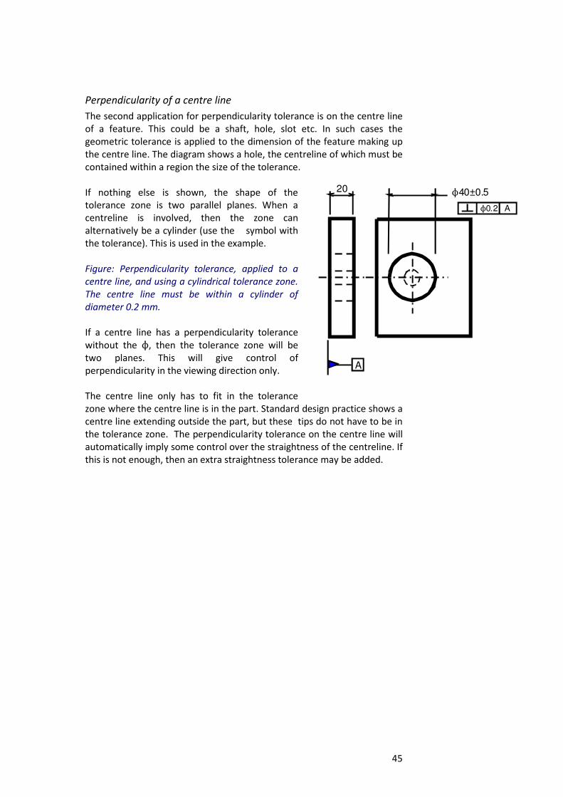
45
Perpendicularity of a centre line
The second application for perpendicularity tolerance is on the centre line
of a feature. This could be a shaft, hole, slot etc. In such cases the
geometric tolerance is applied to the dimension of the feature making up
the centre line. The diagram shows a hole, the centreline of which must be
contained within a region the size of the tolerance.
If nothing else is shown, the shape of the
tolerance zone is two parallel planes. When a
centreline is involved, then the zone can
alternatively be a cylinder (use the symbol with
the tolerance). This is used in the example.
Figure: Perpendicularity tolerance, applied to a
centre line, and using a cylindrical tolerance zone.
The centre line must be within a cylinder of
diameter 0.2 mm.
If a centre line has a perpendicularity tolerance
without the N, then the tolerance zone will be
two planes. This will give control of
perpendicularity in the viewing direction only.
The centre line only has to fit in the tolerance
zone where the centre line is in the part. Standard design practice shows a
centre line extending outside the part, but these tips do not have to be in
the tolerance zone. The perpendicularity tolerance on the centre line will
automatically imply some control over the straightness of the centreline. If
this is not enough, then an extra straightness tolerance may be added.
AN0.2
A
N40±0.520
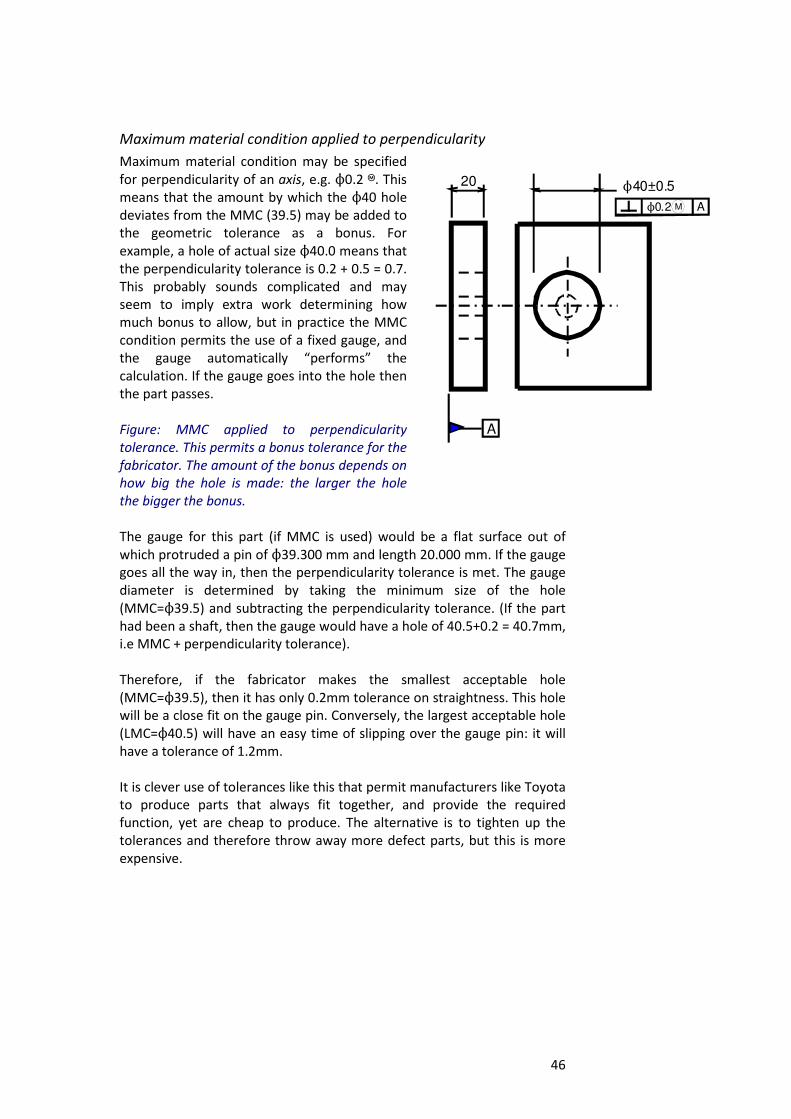
46
Maximum material condition applied to perpendicularity
Maximum material condition may be specified
for perpendicularity of an axis, e.g. N0.2 g. This
means that the amount by which the N40 hole
deviates from the MMC (39.5) may be added to
the geometric tolerance as a bonus. For
example, a hole of actual size N40.0 means that
the perpendicularity tolerance is 0.2 + 0.5 = 0.7.
This probably sounds complicated and may
seem to imply extra work determining how
much bonus to allow, but in practice the MMC
condition permits the use of a fixed gauge, and
the gauge automatically “performs” the
calculation. If the gauge goes into the hole then
the part passes.
Figure: MMC applied to perpendicularity
tolerance. This permits a bonus tolerance for the
fabricator. The amount of the bonus depends on
how big the hole is made: the larger the hole
the bigger the bonus.
The gauge for this part (if MMC is used) would be a flat surface out of
which protruded a pin of N39.300 mm and length 20.000 mm. If the gauge
goes all the way in, then the perpendicularity tolerance is met. The gauge
diameter is determined by taking the minimum size of the hole
(MMC=N39.5) and subtracting the perpendicularity tolerance. (If the part
had been a shaft, then the gauge would have a hole of 40.5+0.2 = 40.7mm,
i.e MMC + perpendicularity tolerance).
Therefore, if the fabricator makes the smallest acceptable hole
(MMC=N39.5), then it has only 0.2mm tolerance on straightness. This hole
will be a close fit on the gauge pin. Conversely, the largest acceptable hole
(LMC=N40.5) will have an easy time of slipping over the gauge pin: it will
have a tolerance of 1.2mm.
It is clever use of tolerances like this that permit manufacturers like Toyota
to produce parts that always fit together, and provide the required
function, yet are cheap to produce. The alternative is to tighten up the
tolerances and therefore throw away more defect parts, but this is more
expensive.
AN0.2
A
N40±0.520
M
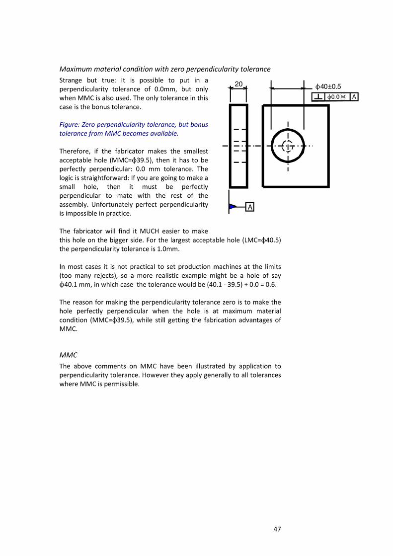
47
Maximum material condition with zero perpendicularity tolerance
Strange but true: It is possible to put in a
perpendicularity tolerance of 0.0mm, but only
when MMC is also used. The only tolerance in this
case is the bonus tolerance.
Figure: Zero perpendicularity tolerance, but bonus
tolerance from MMC becomes available.
Therefore, if the fabricator makes the smallest
acceptable hole (MMC=N39.5), then it has to be
perfectly perpendicular: 0.0 mm tolerance. The
logic is straightforward: If you are going to make a
small hole, then it must be perfectly
perpendicular to mate with the rest of the
assembly. Unfortunately perfect perpendicularity
is impossible in practice.
The fabricator will find it MUCH easier to make
this hole on the bigger side. For the largest acceptable hole (LMC=N40.5)
the perpendicularity tolerance is 1.0mm.
In most cases it is not practical to set production machines at the limits
(too many rejects), so a more realistic example might be a hole of say
N40.1 mm, in which case the tolerance would be (40.1 - 39.5) + 0.0 = 0.6.
The reason for making the perpendicularity tolerance zero is to make the
hole perfectly perpendicular when the hole is at maximum material
condition (MMC=N39.5), while still getting the fabrication advantages of
MMC.
MMC
The above comments on MMC have been illustrated by application to
perpendicularity tolerance. However they apply generally to all tolerances
where MMC is permissible.
AN0.0
A
N40±0.520
M
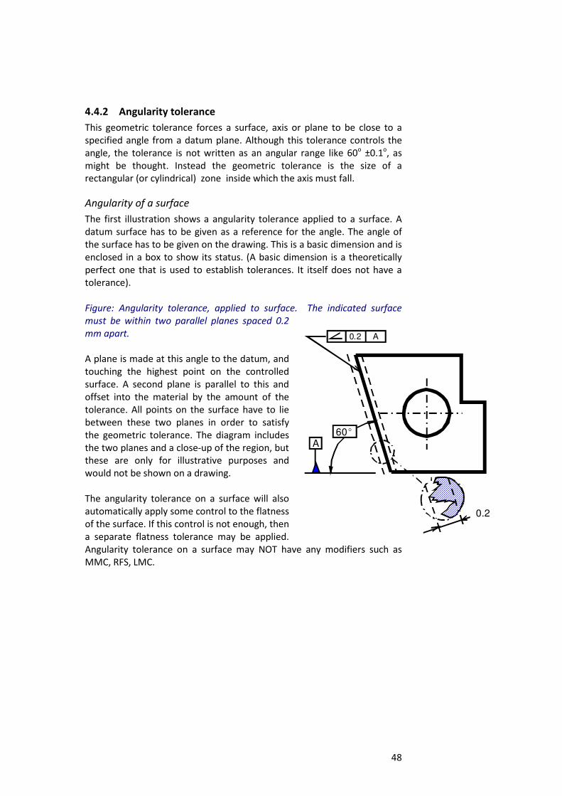
48
4.4.2 Angularity tolerance
This geometric tolerance forces a surface, axis or plane to be close to a
specified angle from a datum plane. Although this tolerance controls the
angle, the tolerance is not written as an angular range like 60o ±0.1
o, as
might be thought. Instead the geometric tolerance is the size of a
rectangular (or cylindrical) zone inside which the axis must fall.
Angularity of a surface
The first illustration shows a angularity tolerance applied to a surface. A
datum surface has to be given as a reference for the angle. The angle of
the surface has to be given on the drawing. This is a basic dimension and is
enclosed in a box to show its status. (A basic dimension is a theoretically
perfect one that is used to establish tolerances. It itself does not have a
tolerance).
Figure: Angularity tolerance, applied to surface. The indicated surface
must be within two parallel planes spaced 0.2
mm apart.
A plane is made at this angle to the datum, and
touching the highest point on the controlled
surface. A second plane is parallel to this and
offset into the material by the amount of the
tolerance. All points on the surface have to lie
between these two planes in order to satisfy
the geometric tolerance. The diagram includes
the two planes and a close-up of the region, but
these are only for illustrative purposes and
would not be shown on a drawing.
The angularity tolerance on a surface will also
automatically apply some control to the flatness
of the surface. If this control is not enough, then
a separate flatness tolerance may be applied.
Angularity tolerance on a surface may NOT have any modifiers such as
MMC, RFS, LMC.
A0.2
A
0.2
60E
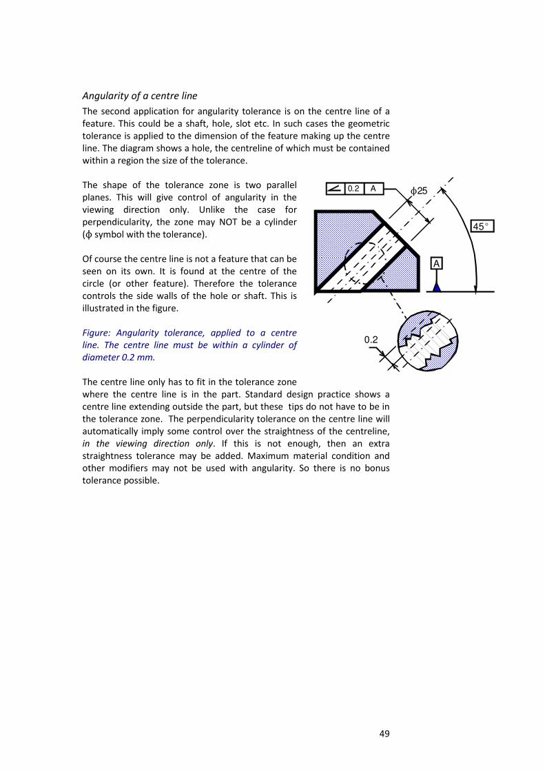
49
Angularity of a centre line
The second application for angularity tolerance is on the centre line of a
feature. This could be a shaft, hole, slot etc. In such cases the geometric
tolerance is applied to the dimension of the feature making up the centre
line. The diagram shows a hole, the centreline of which must be contained
within a region the size of the tolerance.
The shape of the tolerance zone is two parallel
planes. This will give control of angularity in the
viewing direction only. Unlike the case for
perpendicularity, the zone may NOT be a cylinder
(N symbol with the tolerance).
Of course the centre line is not a feature that can be
seen on its own. It is found at the centre of the
circle (or other feature). Therefore the tolerance
controls the side walls of the hole or shaft. This is
illustrated in the figure.
Figure: Angularity tolerance, applied to a centre
line. The centre line must be within a cylinder of
diameter 0.2 mm.
The centre line only has to fit in the tolerance zone
where the centre line is in the part. Standard design practice shows a
centre line extending outside the part, but these tips do not have to be in
the tolerance zone. The perpendicularity tolerance on the centre line will
automatically imply some control over the straightness of the centreline,
in the viewing direction only. If this is not enough, then an extra
straightness tolerance may be added. Maximum material condition and
other modifiers may not be used with angularity. So there is no bonus
tolerance possible.
A0.2
A
45E
N25
0.2
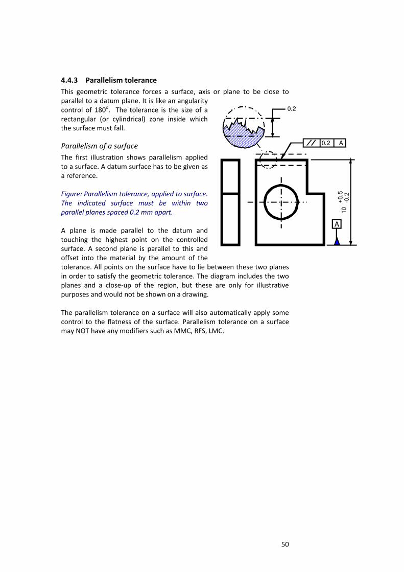
50
4.4.3 Parallelism tolerance
This geometric tolerance forces a surface, axis or plane to be close to
parallel to a datum plane. It is like an angularity
control of 180o. The tolerance is the size of a
rectangular (or cylindrical) zone inside which
the surface must fall.
Parallelism of a surface
The first illustration shows parallelism applied
to a surface. A datum surface has to be given as
a reference.
Figure: Parallelism tolerance, applied to surface.
The indicated surface must be within two
parallel planes spaced 0.2 mm apart.
A plane is made parallel to the datum and
touching the highest point on the controlled
surface. A second plane is parallel to this and
offset into the material by the amount of the
tolerance. All points on the surface have to lie between these two planes
in order to satisfy the geometric tolerance. The diagram includes the two
planes and a close-up of the region, but these are only for illustrative
purposes and would not be shown on a drawing.
The parallelism tolerance on a surface will also automatically apply some
control to the flatness of the surface. Parallelism tolerance on a surface
may NOT have any modifiers such as MMC, RFS, LMC.
0.2 A
A
0.2
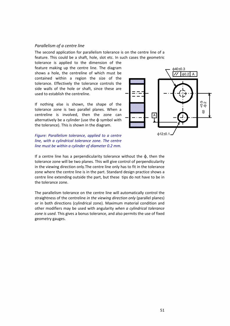
51
AN0.2
A
N40±0.3
N12±0.1
Parallelism of a centre line
The second application for parallelism tolerance is on the centre line of a
feature. This could be a shaft, hole, slot etc. In such cases the geometric
tolerance is applied to the dimension of the
feature making up the centre line. The diagram
shows a hole, the centreline of which must be
contained within a region the size of the
tolerance. Effectively the tolerance controls the
side walls of the hole or shaft, since these are
used to establish the centreline.
If nothing else is shown, the shape of the
tolerance zone is two parallel planes. When a
centreline is involved, then the zone can
alternatively be a cylinder (use the N symbol with
the tolerance). This is shown in the diagram.
Figure: Parallelism tolerance, applied to a centre
line, with a cylindrical tolerance zone. The centre
line must be within a cylinder of diameter 0.2 mm.
If a centre line has a perpendicularity tolerance without the N, then the
tolerance zone will be two planes. This will give control of perpendicularity
in the viewing direction only.The centre line only has to fit in the tolerance
zone where the centre line is in the part. Standard design practice shows a
centre line extending outside the part, but these tips do not have to be in
the tolerance zone.
The parallelism tolerance on the centre line will automatically control the
straightness of the centreline in the viewing direction only (parallel planes)
or in both directions (cylindrical zone). Maximum material condition and
other modifiers may be used with angularity when a cylindrical tolerance
zone is used. This gives a bonus tolerance, and also permits the use of fixed
geometry gauges.
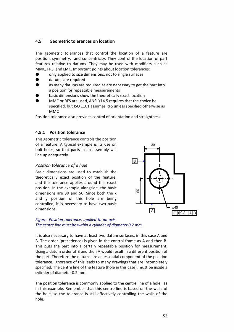
52
N40
30
N0.2 A BA
B
4.5 Geometric tolerances on location
The geometric tolerances that control the location of a feature are
position, symmetry, and concentricity. They control the location of part
features relative to datums. They may be used with modifiers such as
MMC, FRS, and LMC. Important points about location tolerances:
M only applied to size dimensions, not to single surfaces
M datums are required
M as many datums are required as are necessary to get the part into
a position for repeatable measurements
M basic dimensions show the theoretically exact location
M MMC or RFS are used, ANSI Y14.5 requires that the choice be
specified, but ISO 1101 assumes RFS unless specified otherwise as
MMC
Position tolerance also provides control of orientation and straightness.
4.5.1 Position tolerance
This geometric tolerance controls the position
of a feature. A typical example is its use on
bolt holes, so that parts in an assembly will
line up adequately.
Position tolerance of a hole
Basic dimensions are used to establish the
theoretically exact position of the feature,
and the tolerance applies around this exact
position. In the example alongside, the basic
dimensions are 30 and 50. Since both the x
and y position of this hole are being
controlled, it is necessary to have two basic
dimensions.
Figure: Position tolerance, applied to an axis.
The centre line must be within a cylinder of diameter 0.2 mm.
It is also necessary to have at least two datum surfaces, in this case A and
B. The order (precedence) is given in the control frame as A and then B.
This puts the part into a certain repeatable position for measurement.
Using a datum order of B and then A would result in a different position of
the part. Therefore the datums are an essential component of the position
tolerance. Ignorance of this leads to many drawings that are incompletely
specified. The centre line of the feature (hole in this case), must be inside a
cylinder of diameter 0.2 mm.
The position tolerance is commonly applied to the centre line of a hole, as
in this example. Remember that this centre line is based on the walls of
the hole, so the tolerance is still effectively controlling the walls of the
hole.
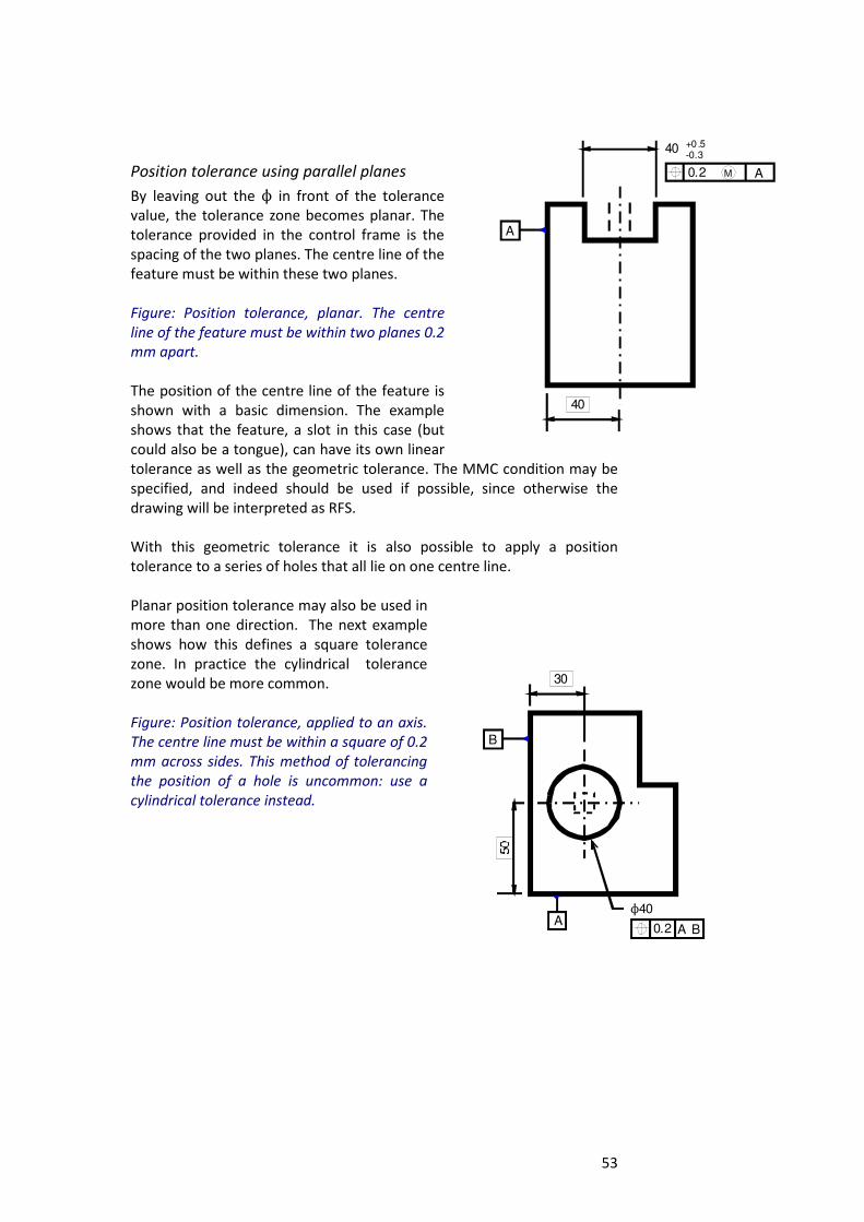
53
Position tolerance using parallel planes
By leaving out the N in front of the tolerance
value, the tolerance zone becomes planar. The
tolerance provided in the control frame is the
spacing of the two planes. The centre line of the
feature must be within these two planes.
Figure: Position tolerance, planar. The centre
line of the feature must be within two planes 0.2
mm apart.
The position of the centre line of the feature is
shown with a basic dimension. The example
shows that the feature, a slot in this case (but
could also be a tongue), can have its own linear
tolerance as well as the geometric tolerance. The MMC condition may be
specified, and indeed should be used if possible, since otherwise the
drawing will be interpreted as RFS.
With this geometric tolerance it is also possible to apply a position
tolerance to a series of holes that all lie on one centre line.
Planar position tolerance may also be used in
more than one direction. The next example
shows how this defines a square tolerance
zone. In practice the cylindrical tolerance
zone would be more common.
Figure: Position tolerance, applied to an axis.
The centre line must be within a square of 0.2
mm across sides. This method of tolerancing
the position of a hole is uncommon: use a
cylindrical tolerance instead.
40
40
0.2 A
A
+0.5-0.3
M
N40
30
0.2 A BA
B
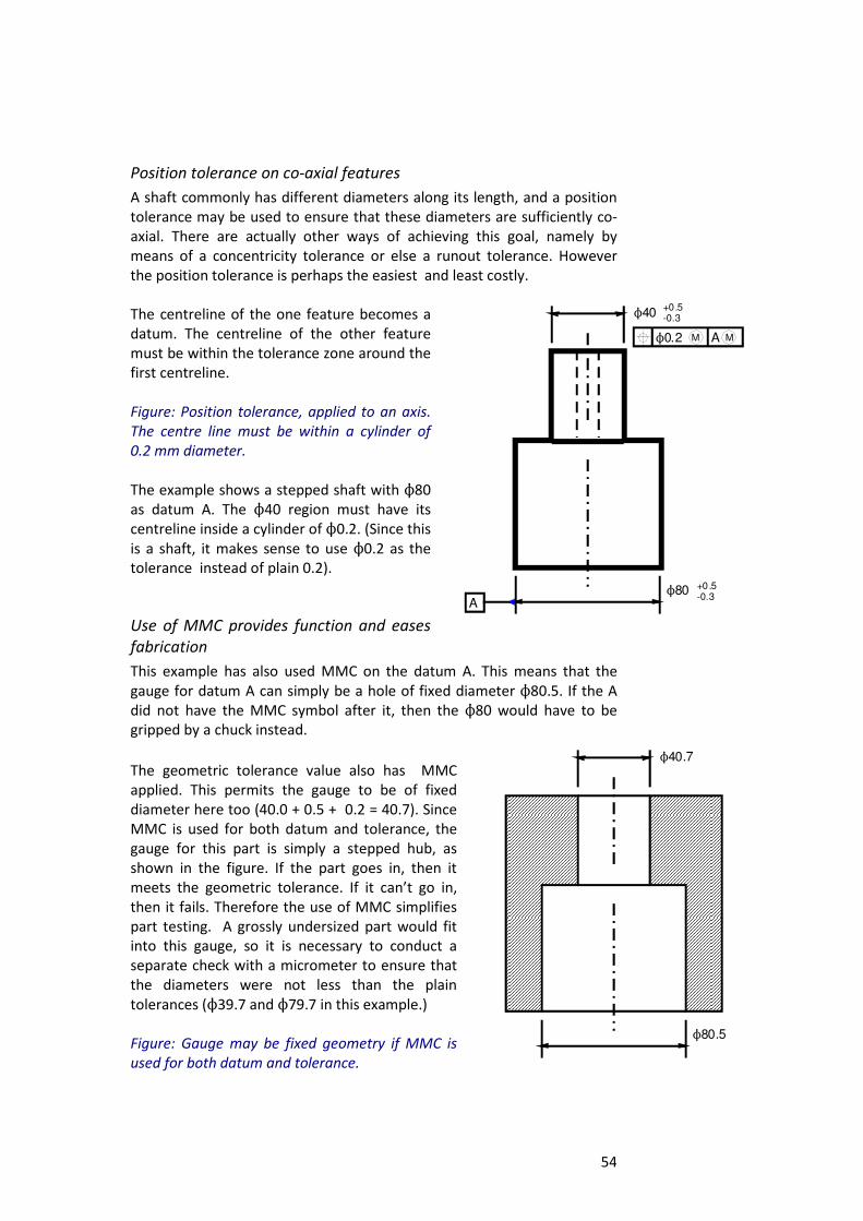
54
Position tolerance on co-axial features
A shaft commonly has different diameters along its length, and a position
tolerance may be used to ensure that these diameters are sufficiently co-
axial. There are actually other ways of achieving this goal, namely by
means of a concentricity tolerance or else a runout tolerance. However
the position tolerance is perhaps the easiest and least costly.
The centreline of the one feature becomes a
datum. The centreline of the other feature
must be within the tolerance zone around the
first centreline.
Figure: Position tolerance, applied to an axis.
The centre line must be within a cylinder of
0.2 mm diameter.
The example shows a stepped shaft with N80
as datum A. The N40 region must have its
centreline inside a cylinder of N0.2. (Since this
is a shaft, it makes sense to use N0.2 as the
tolerance instead of plain 0.2).
Use of MMC provides function and eases
fabrication
This example has also used MMC on the datum A. This means that the
gauge for datum A can simply be a hole of fixed diameter N80.5. If the A
did not have the MMC symbol after it, then the N80 would have to be
gripped by a chuck instead.
The geometric tolerance value also has MMC
applied. This permits the gauge to be of fixed
diameter here too (40.0 + 0.5 + 0.2 = 40.7). Since
MMC is used for both datum and tolerance, the
gauge for this part is simply a stepped hub, as
shown in the figure. If the part goes in, then it
meets the geometric tolerance. If it can’t go in,
then it fails. Therefore the use of MMC simplifies
part testing. A grossly undersized part would fit
into this gauge, so it is necessary to conduct a
separate check with a micrometer to ensure that
the diameters were not less than the plain
tolerances (N39.7 and N79.7 in this example.)
Figure: Gauge may be fixed geometry if MMC is
used for both datum and tolerance.
N40
N80
N0.2 A
A
+0.5-0.3
MM
+0.5-0.3
N40.7
N80.5
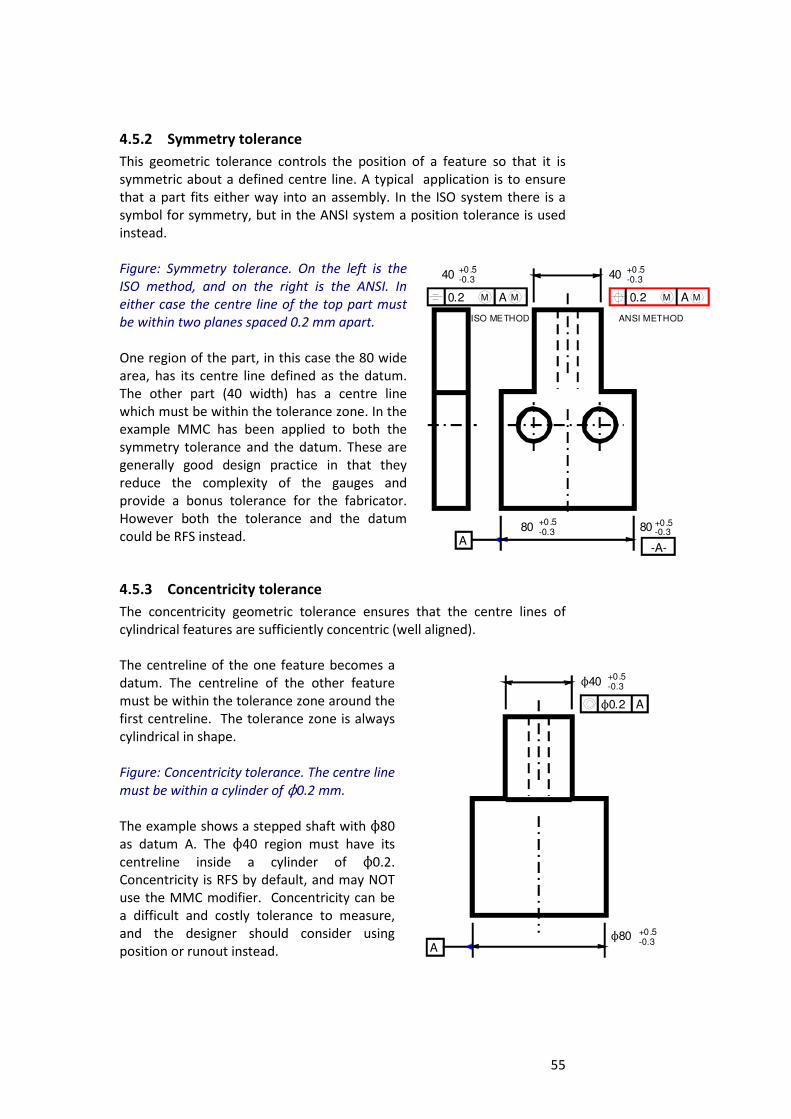
55
4.5.2 Symmetry tolerance
This geometric tolerance controls the position of a feature so that it is
symmetric about a defined centre line. A typical application is to ensure
that a part fits either way into an assembly. In the ISO system there is a
symbol for symmetry, but in the ANSI system a position tolerance is used
instead.
Figure: Symmetry tolerance. On the left is the
ISO method, and on the right is the ANSI. In
either case the centre line of the top part must
be within two planes spaced 0.2 mm apart.
One region of the part, in this case the 80 wide
area, has its centre line defined as the datum.
The other part (40 width) has a centre line
which must be within the tolerance zone. In the
example MMC has been applied to both the
symmetry tolerance and the datum. These are
generally good design practice in that they
reduce the complexity of the gauges and
provide a bonus tolerance for the fabricator.
However both the tolerance and the datum
could be RFS instead.
4.5.3 Concentricity tolerance
The concentricity geometric tolerance ensures that the centre lines of
cylindrical features are sufficiently concentric (well aligned).
The centreline of the one feature becomes a
datum. The centreline of the other feature
must be within the tolerance zone around the
first centreline. The tolerance zone is always
cylindrical in shape.
Figure: Concentricity tolerance. The centre line
must be within a cylinder of N0.2 mm.
The example shows a stepped shaft with N80
as datum A. The N40 region must have its
centreline inside a cylinder of N0.2.
Concentricity is RFS by default, and may NOT
use the MMC modifier. Concentricity can be
a difficult and costly tolerance to measure,
and the designer should consider using
position or runout instead.
40
80
0.2 A
-A-
+0.5-0.3
MM
+0.5-0.3
0.2 A MM
80 +0.5-0.3
A
40+0.5-0.3
ISO METHOD ANSI METHOD
N40
N80
N0.2 A
A
+0.5-0.3
+0.5-0.3
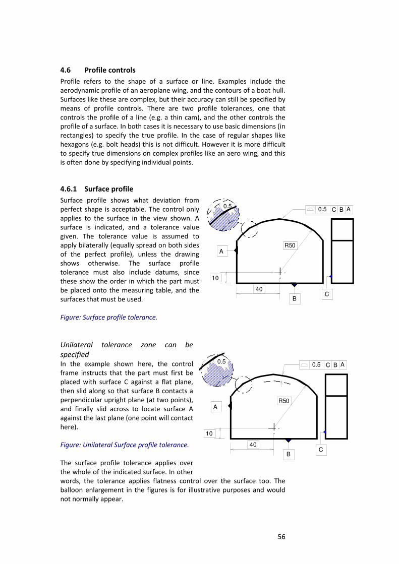
56
4.6 Profile controls
Profile refers to the shape of a surface or line. Examples include the
aerodynamic profile of an aeroplane wing, and the contours of a boat hull.
Surfaces like these are complex, but their accuracy can still be specified by
means of profile controls. There are two profile tolerances, one that
controls the profile of a line (e.g. a thin cam), and the other controls the
profile of a surface. In both cases it is necessary to use basic dimensions (in
rectangles) to specify the true profile. In the case of regular shapes like
hexagons (e.g. bolt heads) this is not difficult. However it is more difficult
to specify true dimensions on complex profiles like an aero wing, and this
is often done by specifying individual points.
4.6.1 Surface profile
Surface profile shows what deviation from
perfect shape is acceptable. The control only
applies to the surface in the view shown. A
surface is indicated, and a tolerance value
given. The tolerance value is assumed to
apply bilaterally (equally spread on both sides
of the perfect profile), unless the drawing
shows otherwise. The surface profile
tolerance must also include datums, since
these show the order in which the part must
be placed onto the measuring table, and the
surfaces that must be used.
Figure: Surface profile tolerance.
Unilateral tolerance zone can be
specified
In the example shown here, the control
frame instructs that the part must first be
placed with surface C against a flat plane,
then slid along so that surface B contacts a
perpendicular upright plane (at two points),
and finally slid across to locate surface A
against the last plane (one point will contact
here).
Figure: Unilateral Surface profile tolerance.
The surface profile tolerance applies over
the whole of the indicated surface. In other
words, the tolerance applies flatness control over the surface too. The
balloon enlargement in the figures is for illustrative purposes and would
not normally appear.
A
0.5 A
B
10
40
R50
BC
C
0.5
A
0.5 A
B
10
40
R50
BC
C
0.5
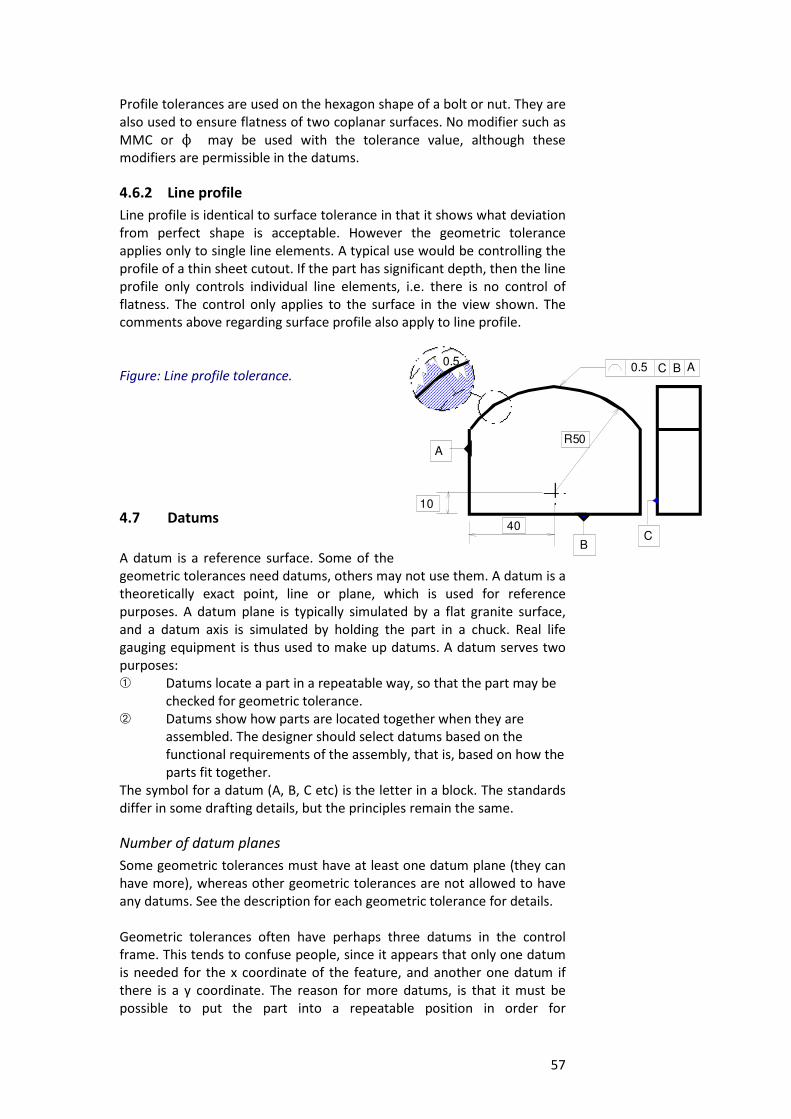
57
A
0.5 A
B
10
40
R50
BC
C
0.5
Profile tolerances are used on the hexagon shape of a bolt or nut. They are
also used to ensure flatness of two coplanar surfaces. No modifier such as
MMC or N may be used with the tolerance value, although these
modifiers are permissible in the datums.
4.6.2 Line profile
Line profile is identical to surface tolerance in that it shows what deviation
from perfect shape is acceptable. However the geometric tolerance
applies only to single line elements. A typical use would be controlling the
profile of a thin sheet cutout. If the part has significant depth, then the line
profile only controls individual line elements, i.e. there is no control of
flatness. The control only applies to the surface in the view shown. The
comments above regarding surface profile also apply to line profile.
Figure: Line profile tolerance.
4.7 Datums
A datum is a reference surface. Some of the
geometric tolerances need datums, others may not use them. A datum is a
theoretically exact point, line or plane, which is used for reference
purposes. A datum plane is typically simulated by a flat granite surface,
and a datum axis is simulated by holding the part in a chuck. Real life
gauging equipment is thus used to make up datums. A datum serves two
purposes:
â Datums locate a part in a repeatable way, so that the part may be
checked for geometric tolerance.
ã Datums show how parts are located together when they are
assembled. The designer should select datums based on the
functional requirements of the assembly, that is, based on how the
parts fit together.
The symbol for a datum (A, B, C etc) is the letter in a block. The standards
differ in some drafting details, but the principles remain the same.
Number of datum planes
Some geometric tolerances must have at least one datum plane (they can
have more), whereas other geometric tolerances are not allowed to have
any datums. See the description for each geometric tolerance for details.
Geometric tolerances often have perhaps three datums in the control
frame. This tends to confuse people, since it appears that only one datum
is needed for the x coordinate of the feature, and another one datum if
there is a y coordinate. The reason for more datums, is that it must be
possible to put the part into a repeatable position in order for
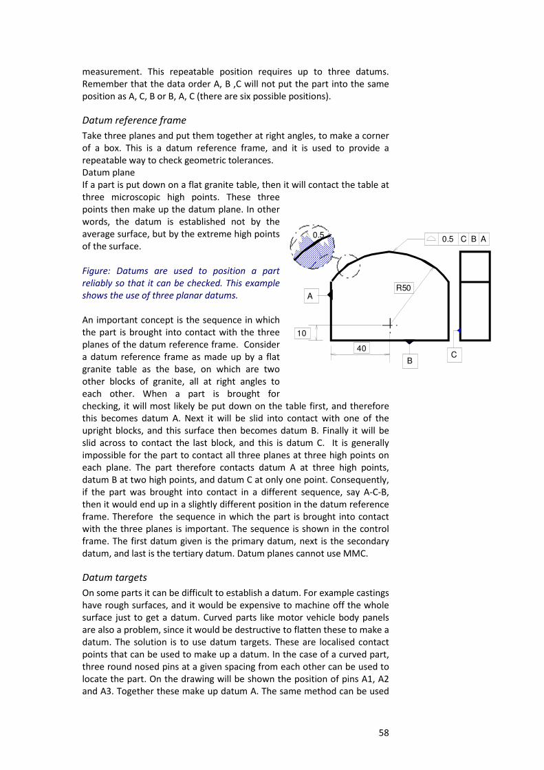
58
measurement. This repeatable position requires up to three datums.
Remember that the data order A, B ,C will not put the part into the same
position as A, C, B or B, A, C (there are six possible positions).
Datum reference frame
Take three planes and put them together at right angles, to make a corner
of a box. This is a datum reference frame, and it is used to provide a
repeatable way to check geometric tolerances.
Datum plane
If a part is put down on a flat granite table, then it will contact the table at
three microscopic high points. These three
points then make up the datum plane. In other
words, the datum is established not by the
average surface, but by the extreme high points
of the surface.
Figure: Datums are used to position a part
reliably so that it can be checked. This example
shows the use of three planar datums.
An important concept is the sequence in which
the part is brought into contact with the three
planes of the datum reference frame. Consider
a datum reference frame as made up by a flat
granite table as the base, on which are two
other blocks of granite, all at right angles to
each other. When a part is brought for
checking, it will most likely be put down on the table first, and therefore
this becomes datum A. Next it will be slid into contact with one of the
upright blocks, and this surface then becomes datum B. Finally it will be
slid across to contact the last block, and this is datum C. It is generally
impossible for the part to contact all three planes at three high points on
each plane. The part therefore contacts datum A at three high points,
datum B at two high points, and datum C at only one point. Consequently,
if the part was brought into contact in a different sequence, say A-C-B,
then it would end up in a slightly different position in the datum reference
frame. Therefore the sequence in which the part is brought into contact
with the three planes is important. The sequence is shown in the control
frame. The first datum given is the primary datum, next is the secondary
datum, and last is the tertiary datum. Datum planes cannot use MMC.
Datum targets
On some parts it can be difficult to establish a datum. For example castings
have rough surfaces, and it would be expensive to machine off the whole
surface just to get a datum. Curved parts like motor vehicle body panels
are also a problem, since it would be destructive to flatten these to make a
datum. The solution is to use datum targets. These are localised contact
points that can be used to make up a datum. In the case of a curved part,
three round nosed pins at a given spacing from each other can be used to
locate the part. On the drawing will be shown the position of pins A1, A2
and A3. Together these make up datum A. The same method can be used
A
0.5 A
B
10
40
R50
BC
C
0.5
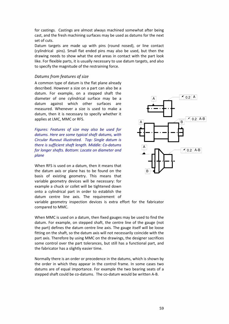
59
for castings. Castings are almost always machined somewhat after being
cast, and the fresh machining surfaces may be used as datums for the next
set of cuts.
Datum targets are made up with pins (round nosed), or line contact
(cylindrical pins). Small flat ended pins may also be used, but then the
drawing needs to show what the end areas in contact with the part look
like. For flexible parts, it is usually necessary to use datum targets, and also
to specify the magnitude of the restraining force.
Datums from features of size
A common type of datum is the flat plane already
described. However a size on a part can also be a
datum. For example, on a stepped shaft the
diameter of one cylindrical surface may be a
datum against which other surfaces are
measured. Whenever a size is used to make a
datum, then it is necessary to specify whether it
applies at LMC, MMC or RFS.
Figures: Features of size may also be used for
datums. Here are some typical shaft datums, with
Circular Runout illustrated. Top: Single datum is
there is sufficient shaft length. Middle: Co-datums
for longer shafts. Bottom: Locate on diameter and
plane
When RFS is used on a datum, then it means that
the datum axis or plane has to be found on the
basis of existing geometry. This means that
variable geometry devices will be necessary: for
example a chuck or collet will be tightened down
onto a cylindrical part in order to establish the
datum centre line axis. The requirement of
variable geometry inspection devices is extra effort for the fabricator
compared to MMC.
When MMC is used on a datum, then fixed gauges may be used to find the
datum. For example, on stepped shaft, the centre line of the gauge (not
the part) defines the datum centre line axis. The gauge itself will be loose
fitting on the shaft, so the datum axis will not necessarily coincide with the
part axis. Therefore by using MMC on the drawings, the designer sacrifices
some control over the part tolerances, but still has a functional part, and
the fabricator has a slightly easier time.
Normally there is an order or precedence in the datums, which is shown by
the order in which they appear in the control frame. In some cases two
datums are of equal importance. For example the two bearing seats of a
stepped shaft could be co-datums. The co-datum would be written A-B.
0.2 A-BB
A
A
A
B
0.2 A-B
0.2 A
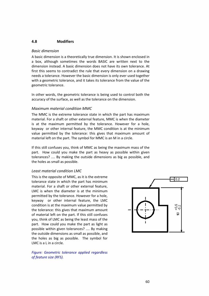
60
4.8 Modifiers
Basic dimension
A basic dimension is a theoretically true dimension. It is shown enclosed in
a box, although sometimes the words BASIC are written next to the
dimension instead. A basic dimension does not have its own tolerance. At
first this seems to contradict the rule that every dimension on a drawing
needs a tolerance. However the basic dimension is only ever used together
with a geometric tolerance, and it takes its tolerance from the value of the
geometric tolerance.
In other words, the geometric tolerance is being used to control both the
accuracy of the surface, as well as the tolerance on the dimension.
Maximum material condition MMC
The MMC is the extreme tolerance state in which the part has maximum
material. For a shaft or other external feature, MMC is when the diameter
is at the maximum permitted by the tolerance. However for a hole,
keyway or other internal feature, the MMC condition is at the minimum
value permitted by the tolerance: this gives that maximum amount of
material left on the part. The symbol for MMC is an M in a circle.
If this still confuses you, think of MMC as being the maximum mass of the
part. How could you make the part as heavy as possible within given
tolerances? .... By making the outside dimensions as big as possible, and
the holes as small as possible.
Least material condition LMC
This is the opposite of MMC, as it is the extreme
tolerance state in which the part has minimum
material. For a shaft or other external feature,
LMC is when the diameter is at the minimum
permitted by the tolerance. However for a hole,
keyway or other internal feature, the LMC
condition is at the maximum value permitted by
the tolerance: this gives that maximum amount
of material left on the part. If this still confuses
you, think of LMC as being the least mass of the
part. How could you make the part as light as
possible within given tolerances? .... By making
the outside dimensions as small as possible, and
the holes as big as possible. The symbol for
LMC is a L in a circle.
Figure: Geometric tolerance applied regardless
of feature size (RFS).
0.2
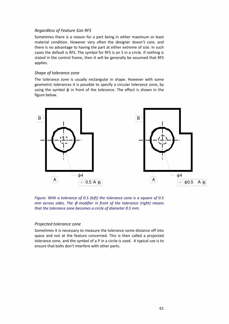
61
Regardless of Feature Size RFS
Sometimes there is a reason for a part being in either maximum or least
material condition. However very often the designer doesn’t care, and
there is no advantage to having the part at either extreme of size. In such
cases the default is RFS. The symbol for RFS is an S in a circle. If nothing is
stated in the control frame, then it will be generally be assumed that RFS
applies.
Shape of tolerance zone
The tolerance zone is usually rectangular in shape. However with some
geometric tolerances it is possible to specify a circular tolerance zone, by
using the symbol N in front of the tolerance. The effect is shown in the
figure below.
Figure: With a tolerance of 0.5 (left) the tolerance zone is a square of 0.5
mm across sides. The N modifier in front of the tolerance (right) means
that the tolerance zone becomes a circle of diameter 0.5 mm.
Projected tolerance zone
Sometimes it is necessary to measure the tolerance some distance off into
space and not at the feature concerned. This is then called a projected
tolerance zone, and the symbol of a P in a circle is used. A typical use is to
ensure that bolts don’t interfere with other parts.
N4
N0.5 A BA
B
N4
0.5 A BA
B
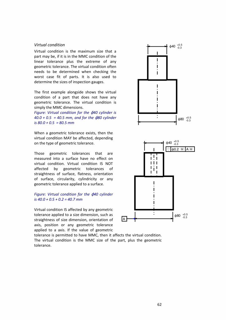
62
Virtual condition
Virtual condition is the maximum size that a
part may be, if it is in the MMC condition of the
linear tolerance plus the extreme of any
geometric tolerance. The virtual condition often
needs to be determined when checking the
worst case fit of parts. It is also used to
determine the sizes of inspection gauges.
The first example alongside shows the virtual
condition of a part that does not have any
geometric tolerance. The virtual condition is
simply the MMC dimensions.
Figure: Virtual condition for the N40 cylinder is
40.0 + 0.5 = 40.5 mm, and for the N80 cylinder
is 80.0 + 0.5 = 80.5 mm
When a geometric tolerance exists, then the
virtual condition MAY be affected, depending
on the type of geometric tolerance.
Those geometric tolerances that are
measured into a surface have no effect on
virtual condition. Virtual condition IS NOT
affected by geometric tolerances of
straightness of surface, flatness, orientation
of surface, circularity, cylindricity or any
geometric tolerance applied to a surface.
Figure: Virtual condition for the N40 cylinder
is 40.0 + 0.5 + 0.2 = 40.7 mm
Virtual condition IS affected by any geometric
tolerance applied to a size dimension, such as
straightness of size dimension, orientation of
axis, position or any geometric tolerance
applied to a axis. If the value of geometric
tolerance is permitted to have MMC, then it affects the virtual condition.
The virtual condition is the MMC size of the part, plus the geometric
tolerance.
N40
N80
N0.2 A
A
+0.5-0.3
MM
+0.5-0.3
N40
N80
+0.5-0.3
+0.5-0.3
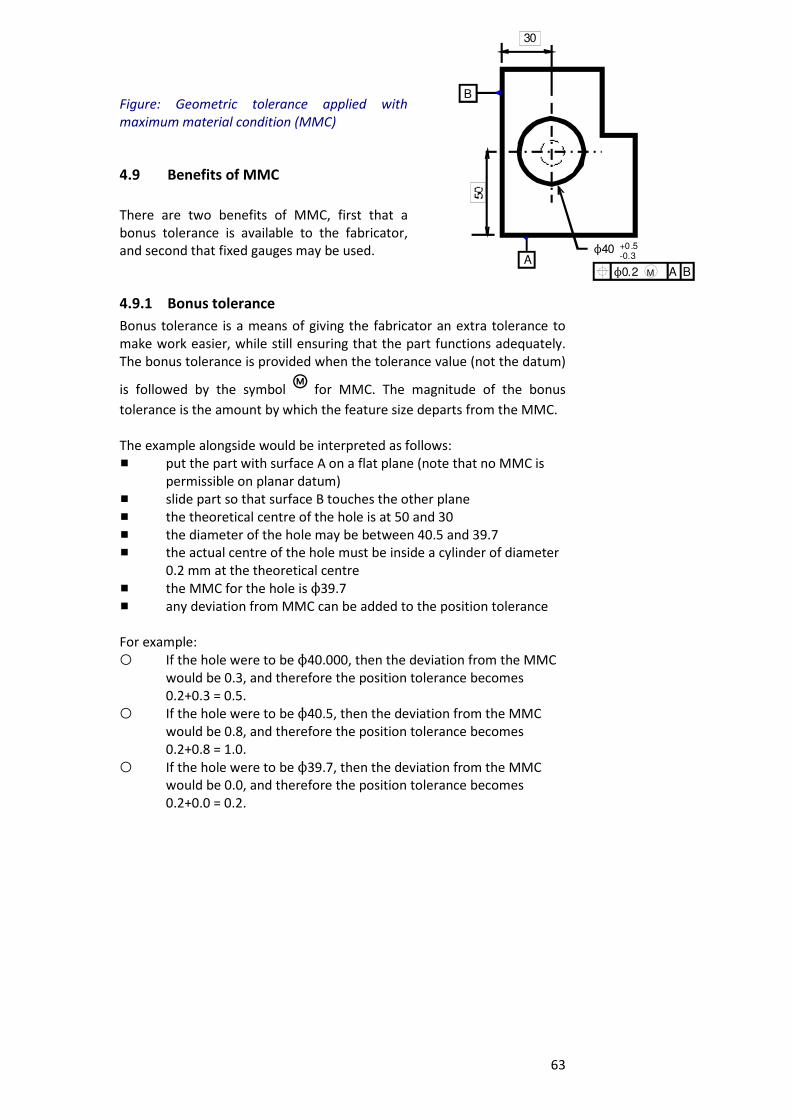
63
Figure: Geometric tolerance applied with
maximum material condition (MMC)
4.9 Benefits of MMC
There are two benefits of MMC, first that a
bonus tolerance is available to the fabricator,
and second that fixed gauges may be used.
4.9.1 Bonus tolerance
Bonus tolerance is a means of giving the fabricator an extra tolerance to
make work easier, while still ensuring that the part functions adequately.
The bonus tolerance is provided when the tolerance value (not the datum)
is followed by the symbol g for MMC. The magnitude of the bonus
tolerance is the amount by which the feature size departs from the MMC.
The example alongside would be interpreted as follows:
# put the part with surface A on a flat plane (note that no MMC is
permissible on planar datum)
# slide part so that surface B touches the other plane
# the theoretical centre of the hole is at 50 and 30
# the diameter of the hole may be between 40.5 and 39.7
# the actual centre of the hole must be inside a cylinder of diameter
0.2 mm at the theoretical centre
# the MMC for the hole is N39.7
# any deviation from MMC can be added to the position tolerance
For example:
F If the hole were to be N40.000, then the deviation from the MMC
would be 0.3, and therefore the position tolerance becomes
0.2+0.3 = 0.5.
F If the hole were to be N40.5, then the deviation from the MMC
would be 0.8, and therefore the position tolerance becomes
0.2+0.8 = 1.0.
F If the hole were to be N39.7, then the deviation from the MMC
would be 0.0, and therefore the position tolerance becomes
0.2+0.0 = 0.2.
N40
30
N0.2 A BA
B
+0.5-0.3
M
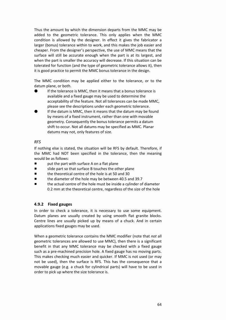
64
Thus the amount by which the dimension departs from the MMC may be
added to the geometric tolerance. This only applies when the MMC
condition is allowed by the designer. In effect it gives the fabricator a
larger (bonus) tolerance within to work, and this makes the job easier and
cheaper. From the designer’s perspective, the use of MMC means that the
surface will still be accurate enough when the part is at its largest, and
when the part is smaller the accuracy will decrease. If this situation can be
tolerated for function (and the type of geometric tolerance allows it), then
it is good practice to permit the MMC bonus tolerance in the design.
The MMC condition may be applied either to the tolerance, or to the
datum plane, or both.
M If the tolerance is MMC, then it means that a bonus tolerance is
available and a fixed gauge may be used to determine the
acceptability of the feature. Not all tolerances can be made MMC,
please see the descriptions under each geometric tolerance.
M If the datum is MMC, then it means that the datum may be found
by means of a fixed instrument, rather than one with movable
geometry. Consequently the bonus tolerance permits a datum
shift to occur. Not all datums may be specified as MMC. Planar
datums may not, only features of size.
RFS
If nothing else is stated, the situation will be RFS by default. Therefore, if
the MMC had NOT been specified in the tolerance, then the meaning
would be as follows:
# put the part with surface A on a flat plane
# slide part so that surface B touches the other plane
# the theoretical centre of the hole is at 50 and 30
# the diameter of the hole may be between 40.5 and 39.7
# the actual centre of the hole must be inside a cylinder of diameter
0.2 mm at the theoretical centre, regardless of the size of the hole
4.9.2 Fixed gauges
In order to check a tolerance, it is necessary to use some equipment.
Datum planes are usually created by using smooth flat granite blocks.
Centre lines are usually picked up by means of a chuck. And in certain
applications fixed gauges may be used.
When a geometric tolerance contains the MMC modifier (note that not all
geometric tolerances are allowed to use MMC), then there is a significant
benefit in that any MMC tolerance may be checked with a fixed gauge
such as a pre-machined precision hole. A fixed gauge has no moving parts.
This makes checking much easier and quicker. If MMC is not used (or may
not be used), then the surface is RFS. This has the consequence that a
movable gauge (e.g. a chuck for cylindrical parts) will have to be used in
order to pick up where the size tolerance is.
65
N40
30
N0.2 A BA
B
+0.5-0.3
M
Maximum material condition (MMC)
The MMC modifier may be used with for example
a position tolerance, and it frees up an additional
bonus tolerance. The bonus is the amount by
which the feature size departs from MMC, and
this is added to the given position tolerance to
determine the total tolerance allowed. If the
feature is at MMC, then there is no bonus
tolerance, and only the given position tolerance
will apply. The bigger the hole (or smaller the
shaft) the greater the bonus tolerance. For the
example shown alongside, the MMC for the hole
is 39.7. If the diameter of the hole is say 40.000,
then the bonus is 40.0 - 39.7 = 0.3, and this is
added to the position tolerance to give a total
tolerance on position of 0.3 + 0.2 = 0.5.
Figure: Position tolerance with MMC applied to
tolerance value.
This calculation does not have to be done at the time of measuring, since
the gauge automatically takes it into account. The gauge for this part
would have two datum surfaces, and a pin, as shown in the diagram.
The centre of the pin would be positioned at the basic dimensions, and the
diameter of the pin would be determined as follows:
O hole is allowed to be as small as 40.0 -
0.3 = 39.7
O hole has a position tolerance of N 0.2 O
MMC is permitted
O therefore pin diameter is 39.7 - 0.2 =
39.5
Figure: Gauge for position tolerance with MMC
If the part fits onto this gauge then it passes the
geometric tolerance. There would need to be a
separate check that the hole diameter was
within its limits.
The advantage of MMC is that it permits the use
of fixed geometry gauges such as these. This
reduces the cost of measurement. It is good
design practice to use MMC where ever it is
permitted and the design will tolerate it.
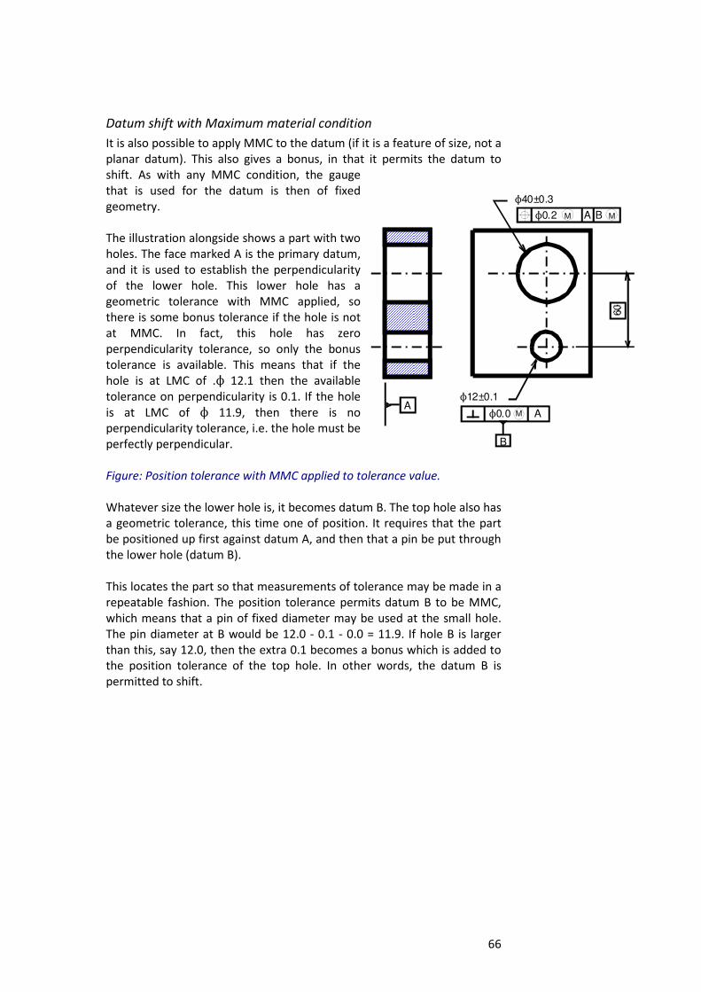
66
Datum shift with Maximum material condition
It is also possible to apply MMC to the datum (if it is a feature of size, not a
planar datum). This also gives a bonus, in that it permits the datum to
shift. As with any MMC condition, the gauge
that is used for the datum is then of fixed
geometry.
The illustration alongside shows a part with two
holes. The face marked A is the primary datum,
and it is used to establish the perpendicularity
of the lower hole. This lower hole has a
geometric tolerance with MMC applied, so
there is some bonus tolerance if the hole is not
at MMC. In fact, this hole has zero
perpendicularity tolerance, so only the bonus
tolerance is available. This means that if the
hole is at LMC of .N 12.1 then the available
tolerance on perpendicularity is 0.1. If the hole
is at LMC of N 11.9, then there is no
perpendicularity tolerance, i.e. the hole must be
perfectly perpendicular.
Figure: Position tolerance with MMC applied to tolerance value.
Whatever size the lower hole is, it becomes datum B. The top hole also has
a geometric tolerance, this time one of position. It requires that the part
be positioned up first against datum A, and then that a pin be put through
the lower hole (datum B).
This locates the part so that measurements of tolerance may be made in a
repeatable fashion. The position tolerance permits datum B to be MMC,
which means that a pin of fixed diameter may be used at the small hole.
The pin diameter at B would be 12.0 - 0.1 - 0.0 = 11.9. If hole B is larger
than this, say 12.0, then the extra 0.1 becomes a bonus which is added to
the position tolerance of the top hole. In other words, the datum B is
permitted to shift.
AN0.0A
N40±0.3
N12±0.1
M
B
N0.2 A B MM
67
The larger hole has a position tolerance that is given as MMC, so this
permits a bonus as well. Again a fixed diameter pin is therefore allowed.
The pin diameter would be 40.0 - 0.3 - 0.2 = 39.5. The datum shift is not
added in here. But the two pins would be mounted on a plate that kept
them rigidly fixed at 60.0 apart, and the datum shift means that any bonus
obtained on datum B would allow this gauge to move up or down, and this
would ease the position tolerance of the upper hole.
Regardless of feature size
All the above only applies if the tolerance is given as MMC on the drawing.
If it is not, then the hole is RFS. The ANSI system requires that either MMC
or RFS or LMC MUST be specified with a positional tolerance, but ISO
assumes that RFS applies unless specifically stated otherwise. Some
geometric tolerances cannot have any modifier at all.
When a geometric tolerance or a datum is given as RFS, then it requires a
movable jaw type gauge that can accommodate the actual size of the
feature (hence the term regardless of feature size). However the
movableness of the jaws takes up any free play, and therefore there is no
bonus tolerance available. Not only is the gauge more expensive, but the
part has smaller tolerances and is therefore usually more expensive.
The MMC and LMC modifiers may only be applied to size dimensions (also
called features-of-size). They may not be applied to surfaces. Therefore
datums may only be referenced MMC when the datum is a centreline.
Least material condition
It is not common to use LMC on tolerances. One application is to control
minimum wall thickness on castings. The LMC condition gives a bonus
tolerance of the amount by which the size of the feature departs from
LMC. This is just the opposite of MMC. LMC generally requires movable
gauges.
4.10 Conclusions
Geometric tolerances achieve something important: they ensure that parts
assemble together well. Consequently there are less defects at production,
and the assembly process itself is easier. That makes for a less expensive
product, and also one that is better quality. Also, maintenance is easier to
perform, partly because parts are interchangeable, but also because
things fit together easier.
All of this is achieved by the special codes we call geometric tolerances.
They capture the intent of the Design Engineers for product functionality,
and represent it in a way that can be put into action by the Production
Engineers. Specifically, the Production Engineers use the information to
determine which part-features need careful attention, and how much. The
tolerances quantify quality. They also describe how the part will be
measured, and what will constitute a pass (defect).
68
Though the symbols and the concepts of geometric tolerances are
complex, they are well-worth understanding by Design-, Production-, and
Metrology-Engineers. The symbols may look like squiggles to the ignorant,
but they are more important than the geometry itself: given the finished
assembly a competitor can always measure the geometry by inspection,
but information on how to make the parts efficiently is locked away in the
geometric tolerances which can only be seen on the drawing.
Recommended reading: KRUILIKOWSKI A, 1991, Delmar, New York ISBN 0827346948


![[Manuel_Martinez-Pons]_The_Psychology_of_Teaching_( ).pdf](https://img.pdfslide.us/doc/110x75/5695d1751a28ab9b02969d25/manuelmartinez-ponsthepsychologyofteachingbookzzorgpdf.jpg)