Embed Size (px)
Citation preview
Polymorphic Type Inferenceand Abstract Data Types
by
Konstantin Läufer
A dissertation submitted in partial fulfillment ofthe requirements for the degree of
Doctor of Philosophy
Department of Computer ScienceNew York University
July, 1992
ApprovedProfessor Benjamin F. Goldberg
Research Advisor

Konstantin LäuferAll Rights Reserved 1992.

v
Abstract
Many statically-typed programming languages provide anabstract data type
construct, such as the package in Ada, the cluster in CLU, and the module
in Modula2. However, in most of these languages, instances of abstract data
types are not first-class values. Thus they cannot be assigned to a variable,
passed as a function parameter, or returned as a function result.
The higher-order functional language ML has a strong and static type
system with parametric polymorphism. In addition, ML provides type recon-
struction and consequently does not require type declarations for identifiers.
Although the ML module system supports abstract data types, their instanc-
es cannot be used as first-class values for type-theoretic reasons.
In this dissertation, we describe a family of extensions of ML. While re-
taining ML’s static type discipline, type reconstruction, and most of its syn-
tax, we add significant expressive power to the language by incorporating
first-class abstract types as an extension of ML’s free algebraic datatypes. In
particular, we are now able to express
• multiple implementations of a given abstract type,
• heterogeneous aggregates of different implementations of the same ab-stract type, and
• dynamic dispatching of operations with respect to the implementationtype.
Following Mitchell and Plotkin, we formalize abstract types in terms of ex-
istentially quantified types. We prove that our type system is semantically
sound with respect to a standard denotational semantics.
We then present an extension of Haskell, a non-strict functional language
that uses type classes to capture systematic overloading. This language re-
sults from incorporating existentially quantified types into Haskell and
gives us first-class abstract types with type classes as their interfaces. We
can now express heterogeneous structures over type classes. The language
is statically typed and offers comparable flexibility to object-oriented lan-
vi
guages. Its semantics is defined through a type-preserving translation to a
modified version of our ML extension.
We have implemented a prototype of an interpreter for our language, in-
cluding the type reconstruction algorithm, in Standard ML.

vii
In memory of my grandfather.

viii
ix
Acknowledgments
First and foremost, I would like to thank my advisors Ben Goldberg and
Martin Odersky. Without their careful guidance and conscientious reading,
this thesis would not have been possible. My work owes a great deal to the
insights and ideas Martin shared with me in numerous stimulating and pro-
ductive discussions. Special thanks go to Fritz Henglein, who introduced me
to the field of type theory and got me on the right track with my research.
I would also like to thank my other committee members, Robert Dewar,
Malcolm Harrison, and Ed Schonberg, for their support and helpful sugges-
tions; the students in the NYU Griffin group for stimulating discussions; and
Franco Gasperoni, Zvi Kedem, Bob Paige, Marco Pellegrini, Dennis Shasha,
John Turek, and Alexander Tuzhilin for valuable advice.
My work has greatly benefited from discussions with Martin Adabi, Ste-
fan Kaes, Tobias Nipkow, Ross Paterson, and Phil Wadler.
Lennart Augustsson promptly incorporated the extensions presented in
this thesis into his solid Haskell implementation. His work made it possible
for me to develop and test example programs.
I would sincerely like to thank all my friends in New York, who made
this city an interesting, inspiring, and enjoyable place to live and work. This
circle of special friends is the part of New York I will miss the most.
My sister Julia, my parents, my grandmother, and numerous friends came
to visit me from far away. Their visits always made me feel close to home,
as did sharing an apartment with my old friend Ingo during my last year in
New York.
Elena has given me great emotional support through her love, patience,
and understanding. She has kept my spirits up during critical phases at work
and elsewhere.
Finally, I would like to thank my parents, who have inspired me through
their own achievements, their commitment to education, their constant en-
couragement and support, and their confidence in me.
x
I dedicate this thesis to my grandfather, Heinrich Viesel. Although it has
now been eight years that he is no longer with me, I want to thank him for
giving me an enthusiasm to learn and for spending many wonderful times
with me.
This research was supported in part by the Defense Advanced Research
Project Agency under Office of Naval Research grants N00014-90-J1110
and N00014-91-5-1472.
xi
Contents
1 Introduction 1
1.1 Objectives . . . . . . . . . . . . . . . . . . . . . . . . . . . . . . . .. . . . . . . . . 1
1.2 Approach. . . . . . . . . . . . . . . . . . . . . . . . . . . . . . . . .. . . . . . . . . 2
1.3 Dissertation Outline. . . . . . . . . . . . . . . . . . . . . . . . .. . . . . . . . . 3
2 Preliminaries 7
2.1 The Languages ML and Haskell . . . . . . . . . . . . . . . .. . . . . . . . . 7
2.1.1 ML . . . . . . . . . . . . . . . . . . . . . . . . . . . . . . . .. . . . . . . . . 7
2.1.2 Shortcomings of Abstract Type Constructs in ML . . . . . 11
2.1.3 Haskell . . . . . . . . . . . . . . . . . . . . . . . . . . . . .. . . . . . . . 15
2.2 The Lambda Calculus, Polymorphism, and Existential Quantifica-
tion . . . . . . . . . . . . . . . . . . . . . . . . . . . . . . . . . . . . .. . . . . . . . 18
2.2.1 The Untypedλ-calculus. . . . . . . . . . . . . . . . .. . . . . . . . 18
2.2.2 The Simply Typedλ-Calculus . . . . . . . . . . . .. . . . . . . . 21
2.2.3 The Typedλ-Calculus withlet -Polymorphism . . . . . . . 23
2.2.4 Higher-Order Typedλ-Calculi . . . . . . . . . . . .. . . . . . . . 26
2.2.5 Existential Quantification . . . . . . . . . . . . . . .. . . . . . . . 26
2.3 Type Reconstruction . . . . . . . . . . . . . . . . . . . . . . . .. . . . . . . . 27
2.3.1 Type Reconstruction for ML . . . . . . . . . . . . .. . . . . . . . 27
2.3.2 Order-Sorted Unification for Haskell . . . . . . .. . . . . . . . 30
xii Contents
2.4 Semantics . . . . . . . . . . . . . . . . . . . . . . . . . . . . . . . . . . . . .. . . 33
2.4.1 Recursive Domains . . . . . . . . . . . . . . . . . . . . . . . . .. . . 33
2.4.2 Weak Ideals . . . . . . . . . . . . . . . . . . . . . . . . . . . . . . .. . . 34
3 An Extension of ML with First-Class Abstract Types 36
3.1 Introduction . . . . . . . . . . . . . . . . . . . . . . . . . . . . . . . . . . . .. . . 36
3.2 Some Motivating Examples . . . . . . . . . . . . . . . . . . . . . . . .. . . 39
3.2.1 Minimum over a Heterogeneous List . . . . . . . . . . . .. . . 39
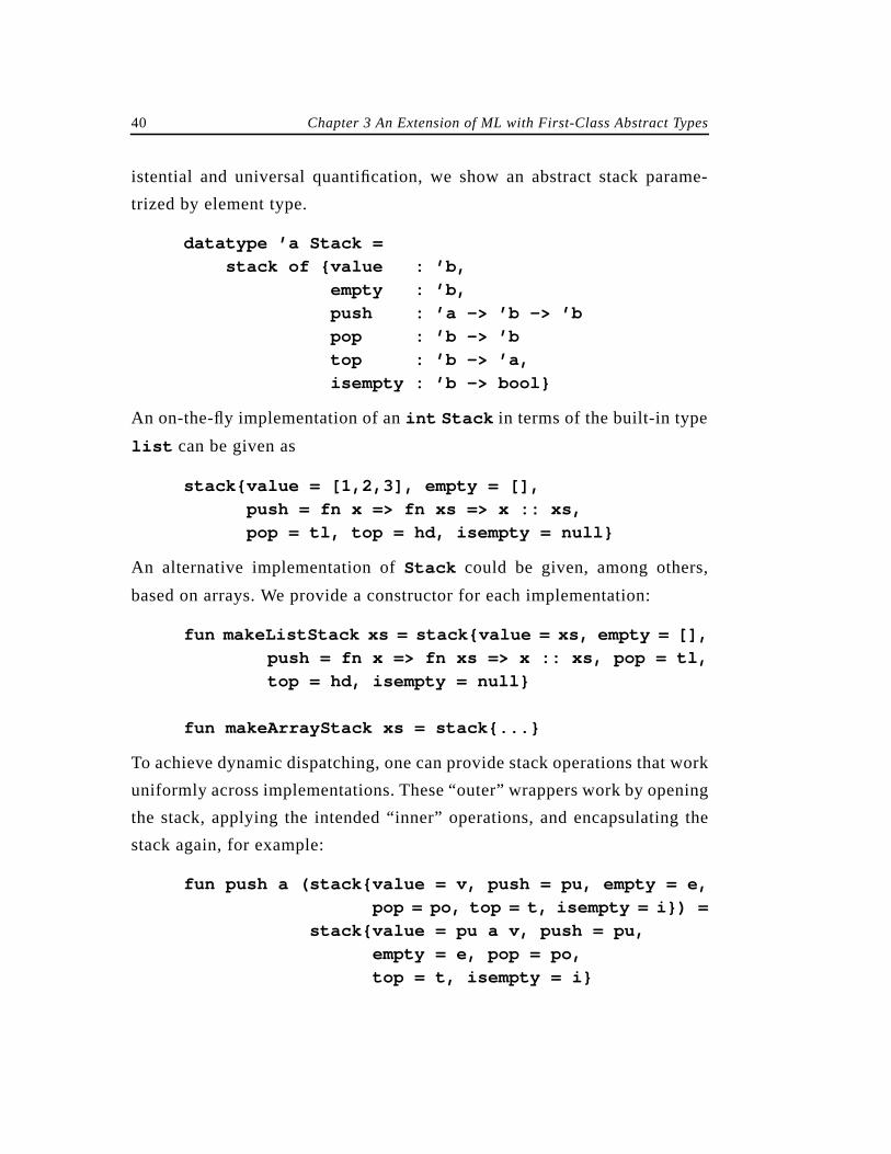
3.2.2 Stacks Parametrized by Element Type . . . . . . . . . . .. . . 39
3.2.3 Squaring a Heterogeneous List of Numbers . . . . . . .. . . 41
3.2.4 Abstract Binary Trees with Equality. . . . . . . . . . . . .. . . 42
3.3 Syntax . . . . . . . . . . . . . . . . . . . . . . . . . . . . . . . . . . . . . . . .. . . 42
3.3.1 Language Syntax . . . . . . . . . . . . . . . . . . . . . . . . . . .. . . 42
3.3.2 Type Syntax. . . . . . . . . . . . . . . . . . . . . . . . . . . . . . .. . . 43
3.4 Type Inference . . . . . . . . . . . . . . . . . . . . . . . . . . . . . . . . . .. . . 44
3.4.1 Instantiation and Generalization of Type Schemes . .. . . 44
3.4.2 Inference Rules for Expressions . . . . . . . . . . . . . . . .. . . 45
3.4.3 Relation to the ML Type Inference System . . . . . . . .. . . 47
3.5 Type Reconstruction . . . . . . . . . . . . . . . . . . . . . . . . . . . . .. . . 48
3.5.1 Auxiliary Functions . . . . . . . . . . . . . . . . . . . . . . . . .. . . 48
3.5.2 Algorithm . . . . . . . . . . . . . . . . . . . . . . . . . . . . . . . .. . . 49
3.5.3 Syntactic Soundness and Completeness of Type Reconstruc-
tion . . . . . . . . . . . . . . . . . . . . . . . . . . . . . . . . . . . . .. . . 50
3.6 Semantics . . . . . . . . . . . . . . . . . . . . . . . . . . . . . . . . . . . . .. . . 56
3.6.1 Semantic Domain . . . . . . . . . . . . . . . . . . . . . . . . . .. . . 57
3.6.2 Semantics of Expressions. . . . . . . . . . . . . . . . . . . . .. . . 57
3.6.3 Semantics of Types . . . . . . . . . . . . . . . . . . . . . . . . .. . . 58
4 An Extension of ML with a Dotless Dot Notation 65
4.1 Introduction . . . . . . . . . . . . . . . . . . . . . . . . . . . . . . . . . . . .. . . 65
Contents xiii
4.2 Some Motivating Examples . . . . . . . . . . . . . . . . . . .. . . . . . . . 66
4.3 Syntax . . . . . . . . . . . . . . . . . . . . . . . . . . . . . . . . . . .. . . . . . . . 68
4.3.1 Language Syntax . . . . . . . . . . . . . . . . . . . . . .. . . . . . . . 68
4.3.2 Type Syntax . . . . . . . . . . . . . . . . . . . . . . . . .. . . . . . . . 69
4.4 Type Inference. . . . . . . . . . . . . . . . . . . . . . . . . . . . .. . . . . . . . 70
4.4.1 Instantiation and Generalization of Type Schemes . . . . . 70
4.4.2 Inference Rules for Expressions. . . . . . . . . . .. . . . . . . . 70
4.5 Type Reconstruction . . . . . . . . . . . . . . . . . . . . . . . .. . . . . . . . 72
4.5.1 Auxiliary Functions. . . . . . . . . . . . . . . . . . . .. . . . . . . . 72
4.5.2 Algorithm . . . . . . . . . . . . . . . . . . . . . . . . . . .. . . . . . . . 72
4.5.3 Syntactic Soundness and Completeness of Type Reconstruc-
tion . . . . . . . . . . . . . . . . . . . . . . . . . . . . . . . .. . . . . . . . 75
4.6 A Translation Semantics . . . . . . . . . . . . . . . . . . . . .. . . . . . . . 75
4.6.1 Modified Original Language . . . . . . . . . . . . .. . . . . . . . 76
4.6.2 Auxiliary Translation Function . . . . . . . . . . .. . . . . . . . 77
4.6.3 Inference-guided Translation . . . . . . . . . . . . .. . . . . . . . 79
4.6.4 Translation of Type Schemes and Assumption Sets . . . . 80
4.6.5 Properties of the Translation . . . . . . . . . . . . .. . . . . . . . 81
5 An Extension of Haskell with First-Class Abstract Types
86
5.1 Introduction. . . . . . . . . . . . . . . . . . . . . . . . . . . . . . .. . . . . . . . 86
5.2 Some Motivating Examples . . . . . . . . . . . . . . . . . . .. . . . . . . . 88
5.2.1 Minimum over a Heterogeneous List . . . . . . .. . . . . . . . 88
5.2.2 Abstract Stack with Multiple Implementations. . . . . . . . 89
5.3 Syntax . . . . . . . . . . . . . . . . . . . . . . . . . . . . . . . . . . .. . . . . . . . 91
5.3.1 Language Syntax . . . . . . . . . . . . . . . . . . . . . .. . . . . . . . 91
5.3.2 Type Syntax . . . . . . . . . . . . . . . . . . . . . . . . .. . . . . . . . 92
5.4 Type Inference. . . . . . . . . . . . . . . . . . . . . . . . . . . . .. . . . . . . . 93
5.4.1 Instantiation and Generalization of Type Schemes . . . . . 93
xiv Contents
5.4.2 Inference Rules for Expressions . . . . . . . . . . . . . . . .. . . 93
5.4.3 Inference Rules for Declarations and Programs . . . .. . . 95
5.4.4 Relation to the Haskell Type Inference System. . . . .. . . 97
5.5 Type Reconstruction . . . . . . . . . . . . . . . . . . . . . . . . . . . . .. . . 97
5.5.1 Unitary Signatures for Principal Types . . . . . . . . . . .. . . 97
5.5.2 Auxiliary Functions . . . . . . . . . . . . . . . . . . . . . . . . .. . . 99
5.5.3 Algorithm . . . . . . . . . . . . . . . . . . . . . . . . . . . . . . . .. . . 99
5.5.4 Syntactic Soundness and Completeness of Type Reconstruc-
tion . . . . . . . . . . . . . . . . . . . . . . . . . . . . . . . . . . . . . . . 102
5.6 Semantics . . . . . . . . . . . . . . . . . . . . . . . . . . . . . . . . . . . . . . . 103
5.6.1 Target Language . . . . . . . . . . . . . . . . . . . . . . . . . . . . . 103
5.6.2 Dictionaries and Translation of Types . . . . . . . . . . . . . 104
5.6.3 Translation Rules for Declarations and Programs . . . . . 107
5.6.4 Translation Rules for Expressions . . . . . . . . . . . . . . . . 108
5.6.5 Properties of the Translation . . . . . . . . . . . . . . . . . . . . 111
6 Related Work, Future Work, and Conclusions 119
6.1 Related Work . . . . . . . . . . . . . . . . . . . . . . . . . . . . . . . . . . . . . 119
6.1.1 SOL . . . . . . . . . . . . . . . . . . . . . . . . . . . . . . . . . . . . . . 120
6.1.2 Hope+C. . . . . . . . . . . . . . . . . . . . . . . . . . . . . . . . . . . . 120
6.1.3 XML+ . . . . . . . . . . . . . . . . . . . . . . . . . . . . . . . . . . . . . 121
6.1.4 Dynamics in ML . . . . . . . . . . . . . . . . . . . . . . . . . . . . . 121
6.1.5 Object-Oriented Languages . . . . . . . . . . . . . . . . . . . . . 121
6.2 Current State of Implementation. . . . . . . . . . . . . . . . . . . . . . . 122
6.3 Conclusions . . . . . . . . . . . . . . . . . . . . . . . . . . . . . . . . . . . . . . 122
6.4 Future Work. . . . . . . . . . . . . . . . . . . . . . . . . . . . . . . . . . . . . . 123
6.4.1 Combination of Modules and Existential Quantification in
ML . . . . . . . . . . . . . . . . . . . . . . . . . . . . . . . . . . . . . . . 123
6.4.2 A Polymorphic Pattern-Matchinglet Expression . . . . 124
Contents xv
6.4.3 Combination of Parameterized Type Classes and Existential
Types in Haskell . . . . . . . . . . . . . . . . . . . . . .. . . . . . . 124
6.4.4 Existential Types and Mutable State . . . . . . .. . . . . . . 124
6.4.5 Full Implementation . . . . . . . . . . . . . . . . . . .. . . . . . . 125
Bibliography 127

xvi Contents
1
1 Introduction
Many statically-typed programming languages provide anabstract data type
construct, such as the package in Ada, the cluster in CLU, and the module
in Modula2. In these languages, an abstract data type consists of two parts,
interface and implementation. The implementation consists of one or more
representation types and someoperations on these types; the interface spec-
ifies thenames and types of the operations accessible to the user of the ab-
stract data type. However, in most of these languages, instances of abstract
data types are not first-class values in the sense that they cannot be assigned
to a variable, passed to a function as a parameter or returned by a function
as a result. Besides, these languages require that types of identifiers be de-
clared explicitly.
1.1 Objectives
This dissertation seeks to answer the following question:
Is it feasible to design a high-level programming language that satis-
fies the following criteria:
1. Strong and static typing: If a program is type-correct, no type errors oc-
cur at runtime.
2. Type reconstruction: Programs need not contain any type declarations
for identifiers; rather, the typings are implicit in the program and can
2 Chapter 1 Introduction
be reconstructed at compile time.
3. Higher-order functional programming: Functions are first-class val-
ues; they may be passed as parameters or returned as results of a func-
tion, and an expression may evaluate to a function.
4. Parametric polymorphism: An expression can have different types de-
pending on the context in which it is used; the set of allowable contexts
is determined by the uniquemost general type of the expression.
5. Extensible abstract types with multiple implementations: The specifi-
cation of an abstract type is separate from its (one or more) implemen-
tations; code written in terms of the specification of an abstract type
applies to any of its implementations; more implementations may be
added later in the program.
6. First-class abstract types: Instances of abstract types are also first-
class values; they can be combined to heterogeneous aggregates of dif-
ferent implementations of the same abstract type.
From a language design point of view, criterion 1 is important for pro-
gramming safety, criteria 2, 3, 4, and 6 are desirable for conciseness and
flexibility of programming, and criterion 5 is crucial for writing reusable li-
braries and extensible systems.
1.2 Approach
The functional language ML [MTH90] already satisfies criteria 1 through 4
fully, and criteria 5 and 6 in a limited, mutually exclusive way. For this rea-
son and for the extensive previous work on the type theory of ML and related
languages, we choose ML as a starting point for our own work.
In this dissertation, we describe a family of extensions of ML. While re-
taining ML’s static type discipline and most of its syntax, we add significant
expressive power to the language by incorporating first-class abstract types
as an extension of ML’s free algebraic datatypes1. The extensions described
Section 1.3 Dissertation Outline 3
are independent of the evaluation strategy of the underlying language; they
apply equally to strict and non-strict languages. In particular, we are now
able to express
• multiple implementations of a given abstract type,
• heterogeneous aggregates of different implementations of the same ab-
stract type, and
• dynamic dispatching of operations with respect to the implementation
type.
Note that a limited form of heterogenicity may already be achieved in
ML by building aggregates over a free algebraic datatype. However, this ap-
proach is not satisfactory because all implementations, corresponding to the
alternatives of the datatype, have to be fixed when the datatype is defined.
Consequently, such a datatype is not extensible and hence useless for the
purpose of, for example, writing a library function that we expect to work
for any future implementation of an abstract type.
ML also features several constructs that provide some form of data ab-
straction. The limitations of these constructs are further discussed in
Chapter 2.
1.3 Dissertation Outline
The chapters in this dissertation are organized as follows:
• Chapter 2. Preliminaries. In this chapter, we review the preliminary
notions and concepts used in the course of the dissertation. First, we
give an overview of the functional languages ML and Haskell and dis-
cuss the shortcomings of data abstraction in ML. Then, we describe the
untyped and several typedλ-calculi and existentially quantified types
as a formal basis for our type-theoretic considerations. Further, we dis-
cuss standard and order-sorted unification algorithms, which are used
1ML’s version of a variant record in Pascal or Ada.
4 Chapter 1 Introduction
in type reconstruction algorithms. Finally, we give a review of domains
and ideals, which we use as a semantic model for the languages we dis-
cuss.
• Chapter 3. An Extension of ML with First-Class Abstract Types.
This chapter presents a semantic extension of ML, where the compo-
nent types of a datatype may be existentially quantified. We show how
datatypes over existential types add significant flexibility to the lan-
guage without even changing ML syntax. We then describe a determin-
istic Damas-Milner type inference system [DM82] [CDDK86] for our
language, which leads to a syntactically sound and complete type re-
construction algorithm. Furthermore, the type system is shown to be
semantically sound with respect to a standard denotational semantics.
• Chapter 4. An Extension of ML with a Dotless Dot Notation.In this
chapter, we describe a further extension of our language. The use of ex-
istential types in connection with an elimination construct (open or
abstype ) is impractical in certain programming situations; this is dis-
cussed in [Mac86]. A formal treatment of the dot notation, an alterna-
tive used in actual programming languages, is found in [CL90]. This
notation assumes the same representation type each time a value of ex-
istential type is accessed, provided that each access is via the same
identifier. We describe an extension of ML with an analogous notation.
A type reconstruction algorithm is given, and semantic soundness is
shown by translating into the language from Chapter 3.
• Chapter 5. An Extension of Haskell with First-Class Abstract
Types.This chapter introduces an extension of the functional language
Haskell [HPJW+92] with existential types. Existential types combine
well with the systematic overloading polymorphism provided by
Haskell type classes [WB89]; this point is first discussed in [LO91].
Briefly, we extend Haskell’sdata declaration in a similar way as the
Section 1.3 Dissertation Outline 5
ML datatype declaration above. In Haskell, it is possible to specify
what type class a (universally quantified) type variable belongs to. In
our extension, we can do the same for existentially quantified type
variables. This lets us use type classes as signatures of abstract data
types; we can then construct heterogeneous aggregates over a given
type class.
• Chapter 6. Related Work, Future Work, and Conclusions.This
chapter concludes with a comparison with related work. Most previous
work on existential types does not consider type reconstruction; other
work that includes type reconstruction seems to be semantically un-
sound. We apparently are the first to permit polymorphic instantiation
of variables of existential type in the body of the elimination construct.
In our system, such variables arelet -bound and therefore polymor-
phic, whereas other work treats them monomorphically. We give an
outlook of future work, which includes further extensions with mutable
state and a practical implementation.
The figure below illustrates the relationship between ML, Haskell, the
languages introduced in this dissertation, and other possible extensions.
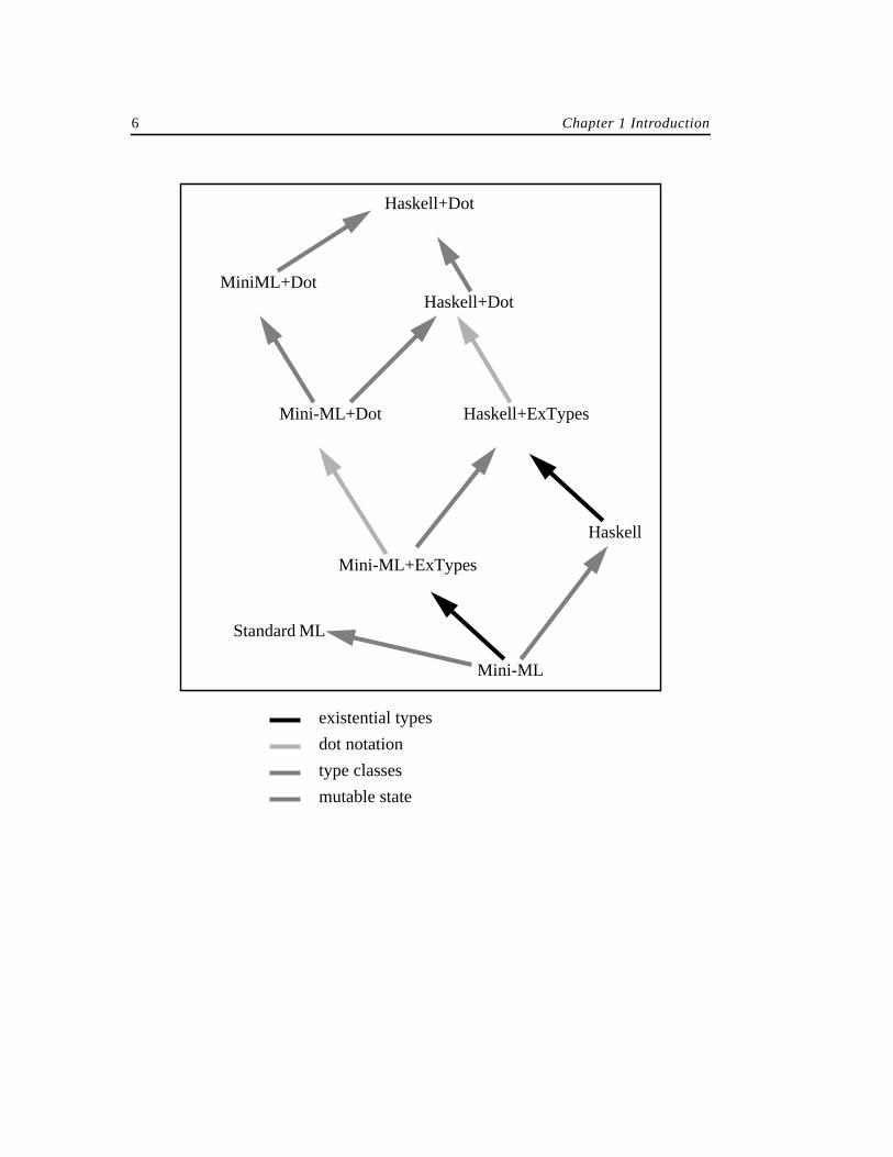
6 Chapter 1 Introduction
Mini-ML
Haskell
Mini-ML+ExTypes
Mini-ML+Dot Haskell+ExTypes
Haskell+DotMiniML+Dot
Haskell+Dot
Standard ML
existential types
dot notation
type classes
mutable state
7
2 Preliminaries
In this chapter, we review the preliminary notions and concepts used in the
course of the dissertation. First, we give an overview of the functional lan-
guages ML and Haskell and discuss in detail the shortcomings of data ab-
straction in ML. Then, we describe the untyped and several typedλ-calculi
and existentially quantified types as a formal basis for our type-theoretic
work below. Further, we discuss standard and order-sorted unification algo-
rithms, which are used in type reconstruction algorithms for implicitly typed
languages. Finally, we give a brief review of domains and ideals, which we
use as a semantic model for the languages we discuss.
2.1 The Languages ML and Haskell
This section gives an overview of the functional languages ML and Haskell
and discusses the shortcomings of the data abstraction constructs provided
by ML. We assume some general background in programming languages;
prior exposure to a statically typed functional language is helpful.
2.1.1 ML
We present a few programming examples that illustrate the relevant core of
ML [MTH90] and its type system. For a full introduction, see [Har90]. The
syntax of core expressions is defined recursively as constants, identifiers,
and three constructs:
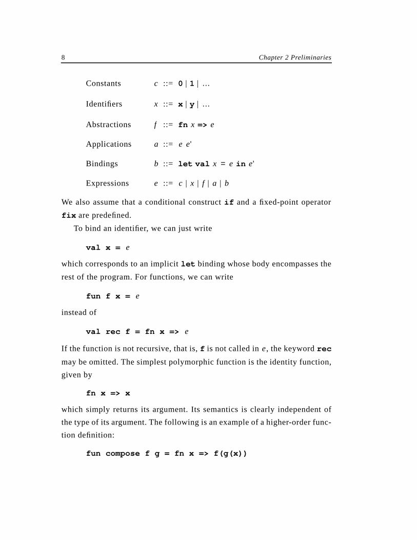
8 Chapter 2 Preliminaries
Constants ::=0 | 1 |
Identifiers ::= x | y |
Abstractions ::= fn =>
Applications ::=
Bindings ::= let val in
Expressions ::= | | | |
We also assume that a conditional constructif and a fixed-point operator
fix are predefined.
To bind an identifier, we can just write
val x =
which corresponds to an implicitlet binding whose body encompasses the
rest of the program. For functions, we can write
fun f x =
instead of
val rec f = fn x =>
If the function is not recursive, that is,f is not called in , the keywordrec
may be omitted. The simplest polymorphic function is the identity function,
given by
fn x => x
which simply returns its argument. Its semantics is clearly independent of
the type of its argument. The following is an example of a higher-order func-
tion definition:
fun compose f g = fn x => f(g(x))
c …
x …
f x e
a e e'
b x e= e'
e c x f a b
e
e
e
e
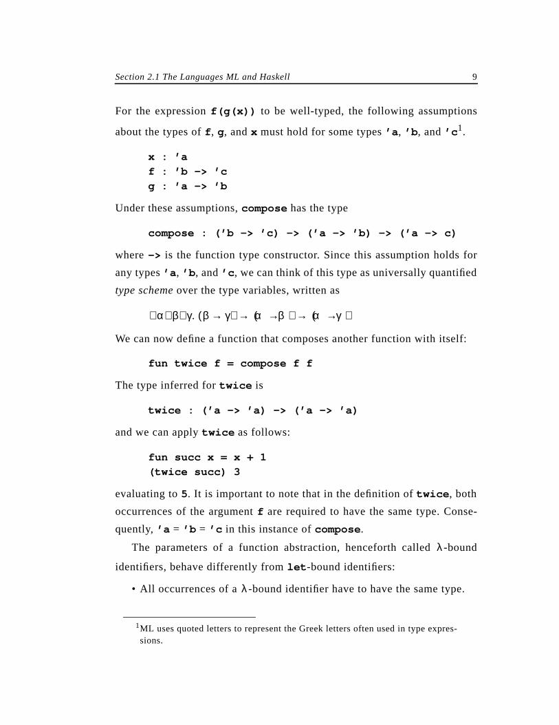
Section 2.1 The Languages ML and Haskell 9
For the expressionf(g(x)) to be well-typed, the following assumptions
about the types off , g, andx must hold for some types’a , ’b , and’c 1.
x : ’a
f : ’b -> ’c
g : ’a -> ’b
Under these assumptions,compose has the type
compose : (’b -> ’c) -> (’a -> ’b) -> (’a -> c)
where-> is the function type constructor. Since this assumption holds for
any types’a , ’b , and’c , we can think of this type as universally quantified
type scheme over the type variables, written as
We can now define a function that composes another function with itself:
fun twice f = compose f f
The type inferred fortwice is
twice : (’a -> ’a) -> (’a -> ’a)
and we can applytwice as follows:
fun succ x = x + 1
(twice succ) 3
evaluating to5. It is important to note that in the definition oftwice , both
occurrences of the argumentf are required to have the same type. Conse-
quently, ’a = ’b = ’c in this instance ofcompose .
The parameters of a function abstraction, henceforth called -bound
identifiers, behave differently fromlet -bound identifiers:
• All occurrences of a -bound identifier have to have the same type.
1ML uses quoted letters to represent the Greek letters often used in type expres-sions.
α β γ∀∀∀ . β γ→( ) α β→( ) α γ→( )→ →
λ
λ
10 Chapter 2 Preliminaries
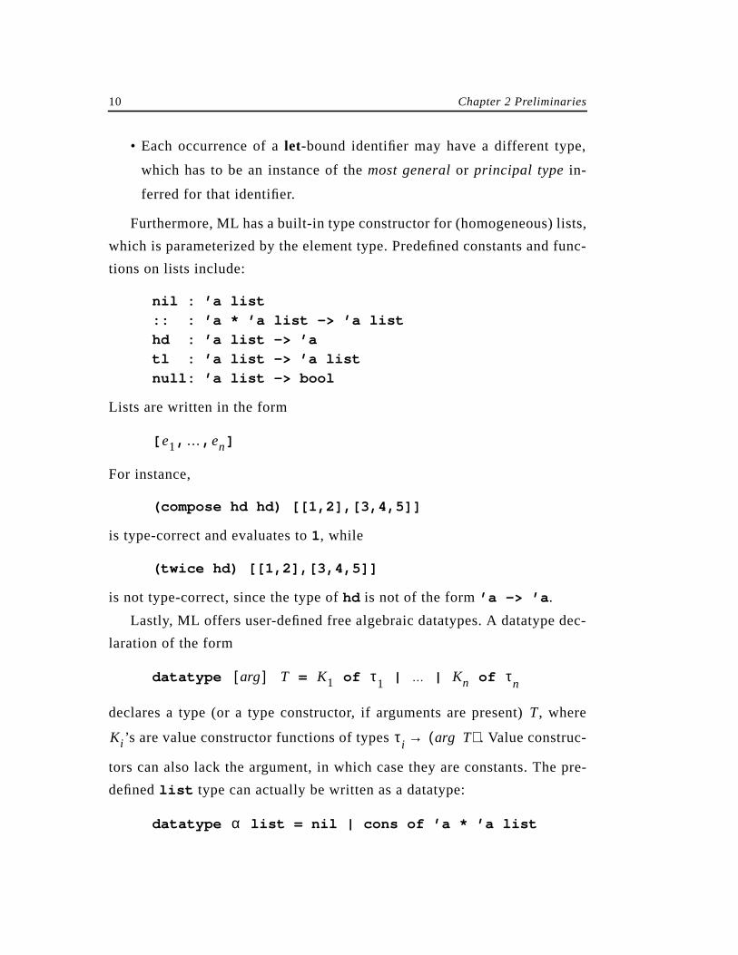
• Each occurrence of alet-bound identifier may have a different type,
which has to be an instance of themost generalor principal type in-
ferred for that identifier.
Furthermore, ML has a built-in type constructor for (homogeneous) lists,
which is parameterized by the element type. Predefined constants and func-
tions on lists include:
nil : ’a list
:: : ’a * ’a list -> ’a list
hd : ’a list -> ’a
tl : ’a list -> ’a list
null: ’a list -> bool
Lists are written in the form
[ , , ]
For instance,
(compose hd hd) [[1,2],[3,4,5]]
is type-correct and evaluates to1, while
(twice hd) [[1,2],[3,4,5]]
is not type-correct, since the type ofhd is not of the form’a -> ’a .
Lastly, ML offers user-defined free algebraic datatypes. A datatype dec-
laration of the form
datatype = of | | of
declares a type (or a type constructor, if arguments are present) , where
’s are value constructor functions of types . Value construc-
tors can also lack the argument, in which case they are constants. The pre-
definedlist type can actually be written as a datatype:
datatype list = nil | cons of ’a * ’a list
e1 … en
arg[ ] T K1 τ1 … Kn τn
T
Ki τi arg T( )→
α
Section 2.1 The Languages ML and Haskell 11
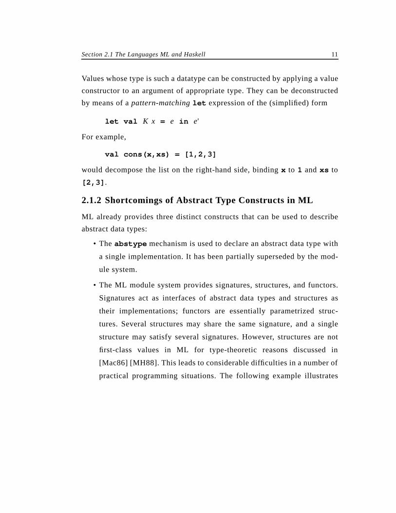
Values whose type is such a datatype can be constructed by applying a value
constructor to an argument of appropriate type. They can be deconstructed
by means of apattern-matchinglet expression of the (simplified) form
let val = in
For example,
val cons(x,xs) = [1,2,3]
would decompose the list on the right-hand side, bindingx to 1 andxs to
[2,3] .
2.1.2 Shortcomings of Abstract Type Constructs in ML
ML already provides three distinct constructs that can be used to describe
abstract data types:
• The abstype mechanism is used to declare an abstract data type with
a single implementation. It has been partially superseded by the mod-
ule system.
• The ML module system provides signatures, structures, and functors.
Signatures act as interfaces of abstract data types and structures as
their implementations; functors are essentially parametrized struc-
tures. Several structures may share the same signature, and a single
structure may satisfy several signatures. However, structures are not
first-class values in ML for type-theoretic reasons discussed in
[Mac86] [MH88]. This leads to considerable difficulties in a number of
practical programming situations. The following example illustrates
K x e e'
12 Chapter 2 Preliminaries
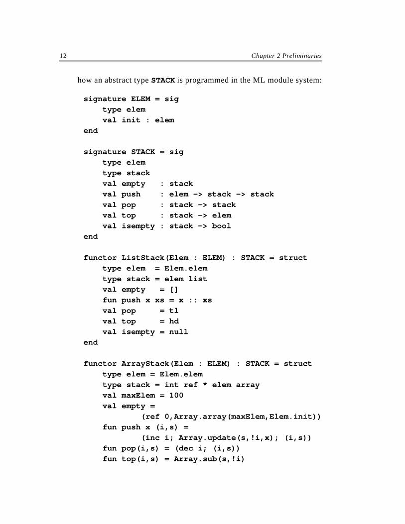
how an abstract typeSTACK is programmed in the ML module system:
signature ELEM = sig
type elem
val init : elem
end
signature STACK = sig
type elem
type stack
val empty : stack
val push : elem -> stack -> stack
val pop : stack -> stack
val top : stack -> elem
val isempty : stack -> bool
end
functor ListStack(Elem : ELEM) : STACK = struct
type elem = Elem.elem
type stack = elem list
val empty = []
fun push x xs = x :: xs
val pop = tl
val top = hd
val isempty = null
end
functor ArrayStack(Elem : ELEM) : STACK = struct
type elem = Elem.elem
type stack = int ref * elem array
val maxElem = 100
val empty =
(ref 0,Array.array(maxElem,Elem.init))
fun push x (i,s) =
(inc i; Array.update(s,!i,x); (i,s))
fun pop(i,s) = (dec i; (i,s))
fun top(i,s) = Array.sub(s,!i)
Section 2.1 The Languages ML and Haskell 13
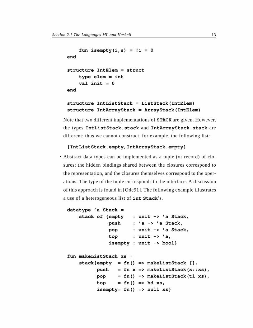
fun isempty(i,s) = !i = 0
end
structure IntElem = struct
type elem = int
val init = 0
end
structure IntListStack = ListStack(IntElem)
structure IntArrayStack = ArrayStack(IntElem)
Note that two different implementations ofSTACK are given. However,
the typesIntListStack.stack and IntArrayStack.stack are
different; thus we cannot construct, for example, the following list:
[IntListStack.empty,IntArrayStack.empty]
• Abstract data types can be implemented as a tuple (or record) of clo-
sures; the hidden bindings shared between the closures correspond to
the representation, and the closures themselves correspond to the oper-
ations. The type of the tuple corresponds to the interface. A discussion
of this approach is found in [Ode91]. The following example illustrates
a use of a heterogeneous list ofint Stack ’s.
datatype ’a Stack =
stack of empty : unit -> ’a Stack,
push : ’a -> ’a Stack,
pop : unit -> ’a Stack,
top : unit -> ’a,
isempty : unit -> bool
fun makeListStack xs =
stackempty = fn() => makeListStack [],
push = fn x => makeListStack(x::xs),
pop = fn() => makeListStack(tl xs),
top = fn() => hd xs,
isempty= fn() => null xs
14 Chapter 2 Preliminaries
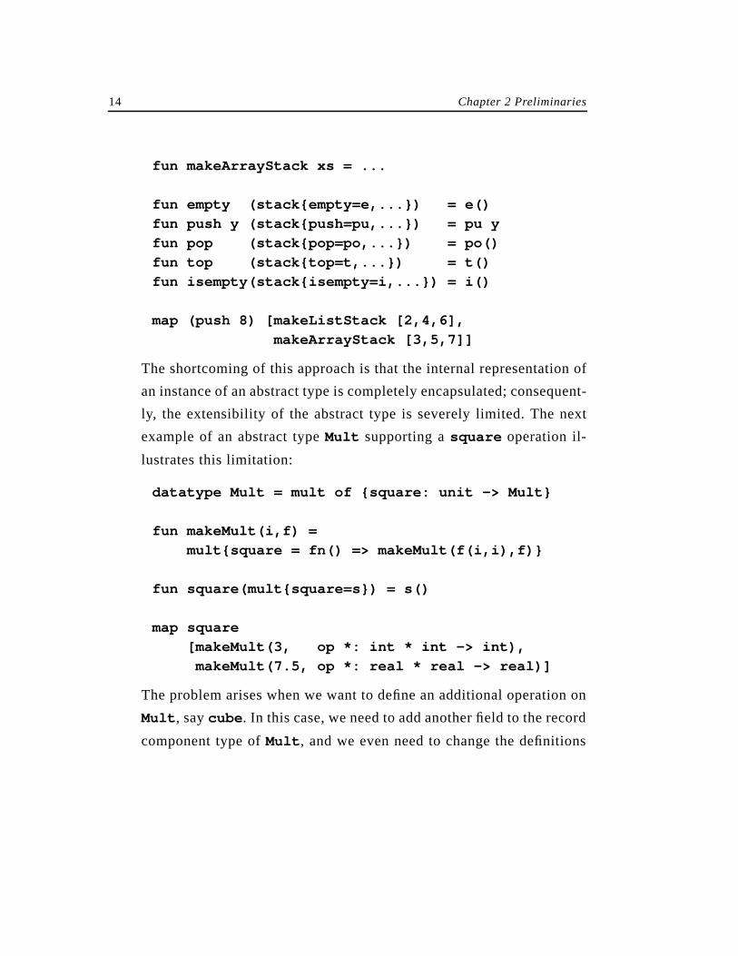
fun makeArrayStack xs = ...
fun empty (stackempty=e,...) = e()
fun push y (stackpush=pu,...) = pu y
fun pop (stackpop=po,...) = po()
fun top (stacktop=t,...) = t()
fun isempty(stackisempty=i,...) = i()
map (push 8) [makeListStack [2,4,6],
makeArrayStack [3,5,7]]
The shortcoming of this approach is that the internal representation of
an instance of an abstract type is completely encapsulated; consequent-
ly, the extensibility of the abstract type is severely limited. The next
example of an abstract typeMult supporting asquare operation il-
lustrates this limitation:
datatype Mult = mult of square: unit -> Mult
fun makeMult(i,f) =
multsquare = fn() => makeMult(f(i,i),f)
fun square(multsquare=s) = s()
map square
[makeMult(3, op *: int * int -> int),
makeMult(7.5, op *: real * real -> real)]
The problem arises when we want to define an additional operation on
Mult , saycube . In this case, we need to add another field to the record
component type ofMult , and we even need to change the definitions
Section 2.1 The Languages ML and Haskell 15
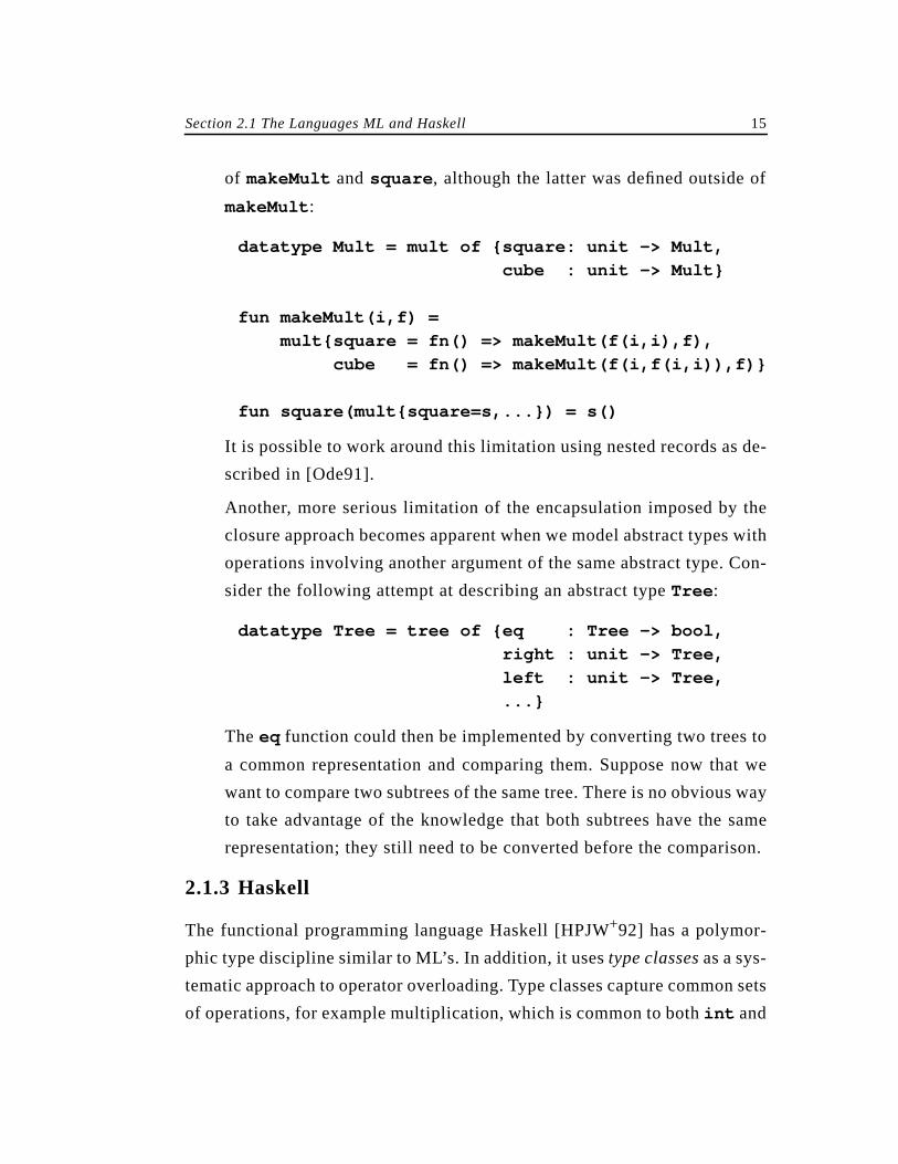
of makeMult andsquare , although the latter was defined outside of
makeMult :
datatype Mult = mult of square: unit -> Mult,
cube : unit -> Mult
fun makeMult(i,f) =
multsquare = fn() => makeMult(f(i,i),f),
cube = fn() => makeMult(f(i,f(i,i)),f)
fun square(multsquare=s,...) = s()
It is possible to work around this limitation using nested records as de-
scribed in [Ode91].
Another, more serious limitation of the encapsulation imposed by the
closure approach becomes apparent when we model abstract types with
operations involving another argument of the same abstract type. Con-
sider the following attempt at describing an abstract typeTree :
datatype Tree = tree of eq : Tree -> bool,
right : unit -> Tree,
left : unit -> Tree,
...
Theeq function could then be implemented by converting two trees to
a common representation and comparing them. Suppose now that we
want to compare two subtrees of the same tree. There is no obvious way
to take advantage of the knowledge that both subtrees have the same
representation; they still need to be converted before the comparison.
2.1.3 Haskell
The functional programming language Haskell [HPJW+92] has a polymor-
phic type discipline similar to ML’s. In addition, it usestype classes as a sys-
tematic approach to operator overloading. Type classes capture common sets
of operations, for example multiplication, which is common to bothint and
16 Chapter 2 Preliminaries
real types. A particular type may be an instance of a type class and has an
operation corresponding to each operation defined in the type class. Further,
type classes may be arranged in a class hierarchy, in the sense that a derived
type class captures all operations of its superclasses and may add new ones.
Type classes were first introduced in the article [WB89], which also gives
additional motivating examples and shows how Haskell programs are trans-
lated to ML programs.
The syntax of the Haskell core consists of essentially the same expres-
sions as the ML core, with the addition of class and instance declarations of
the following form:
class where
::
::
instance where
=
=
To motivate the type class approach, consider the overloading of mathe-
matical operators in ML. Although4*4 and4.7*4.7 are valid ML expres-
sions, we cannot define a function such as
fun square x = x * x
in ML, as the overloading of the operator* cannot be resolved unambigu-
ously. In Haskell, we first declare a classNum to capture the operationsInt
andFloat have in common:
class Num a where
(-) :: a -> a
(+) :: a -> a -> a
(*) :: a -> a -> a
C a
op1 τ1
…opn τn
C t
op1 e1
…opn en
Section 2.1 The Languages ML and Haskell 17
At this point, we can already type thesquare function, although we cannot
use it yet, since we do not have any instances ofNum. The typing is
square :: Num a => a -> a
which reads, “for anya that is an instance ofNum, square has type
a -> a .” We then declare two instances ofNum, assuming the existence of
some predefined functions onInt andFloat :
instance Num Int where
(-) = intUMinus
(+) = intAdd
(*) = intMult
instance Num Float where
(-) = floatUminus
(+) = floatAdd
(*) = floatMult
When we now writesquare 4.0 , the type reconstructor finds out that4.0
is of typeFloat , which in turn is an instance ofNum. The multiplication
used isfloatMult , as specified in the instance declaration forFloat . Giv-
en a definition of the functionmap, we can write the function
squarelist xs = map square xs
which squares each element in a list. It has type
squarelist :: Num a => [a] -> [a]
where[a] is the Haskell version of’a list .
Haskell also provides algebraic datatypes, which differ from the ones in
ML only in that the formal arguments of the type constructor can be speci-
fied to be instances of a certain type class.
It should also be mentioned that Haskell is apure, non-strict functional
language, whereas ML is astrict language and provides mutable state in the
form of references.
18 Chapter 2 Preliminaries
2.2 The Lambda Calculus, Polymorphism, and
Existential Quantification
In this section, we describe the untyped, the simply typed, and the first-order
polymorphic λ-calculi, which constitute the type-theoretic basis for func-
tional languages such as ML and Haskell. We also give an introduction to
existentially quantified types, which provide a type-theoretic description of
abstract data types.
2.2.1 The Untypedλ-calculus
The untypedλ-calculus is a formal model of computation. While theλ-cal-
culus is equivalent to Turing machines in computational power, its simple,
functional structure lends itself as a useful model for reasoning about pro-
grams, in particular, functional programs. We give a brief introduction to the
λ-calculus; a comprehensive reference is [Bar84].
λ-terms are defined as follows:
Constants1
Identifiers
Terms ::= | | |
In a λ-abstraction of the form , where is someλ-term, the variable
is said to bebound in and is called abound variable. Any variable in
other than that is not bound in aλ-abstraction inside is said to occur
free in and is called afree variable. We assume that no free variable is
identical to any bound variable within aλ-term.
Theλ-calculus provides severalconversion rules for transforming oneλ-
term into an equivalent one. The conversion rules are defined as follows:
1Constants are not actually part of thepure λ-calculus, but are a useful enrich-
ment.
c
x
e c x λx.e e e'( )
a λx.e e
x a y
e x e
a
Section 2.2 The Lambda Calculus, Polymorphism, and Existential Quantification 19
• β-conversion:
This rule models function application. It states that aλ-abstraction
is applied to a term by replacing each free occurrence of in
by a copy of . In addition, bound variables in have to be renamed
to avoid name conflict with variables that are free in . stands
for this new term.
• α-conversion:
This rule states that the bound variable of aλ-abstraction may be re-
named, provided that the renamed variable does not occur free in .
• η-conversion:
This rule can be used to eliminate a redundantλ-abstraction, provided
that the bound variable does not occur free in .
• δ-conversion:
The δ-rules define conversion of built-in constants and functions, for
example,
We view the set ofλ-terms as divided intoα-equivalence classes; this means
that any twoλ-terms that can be transformed into one another viaα-conver-
sion are in the same equivalence class, and any one term is viewed as a rep-
resentant of itsα-equivalence class.
λx.e( ) e' e e' x⁄[ ]⇔
λx.e e' x
e e' e
e' e e' x⁄[ ]
λx.e λy.e y x⁄[ ]⇔ y FV e( )∉
e
λx. e x( ) e⇔ x FV e( )∉
e
times3 4( ) 12⇔
20 Chapter 2 Preliminaries
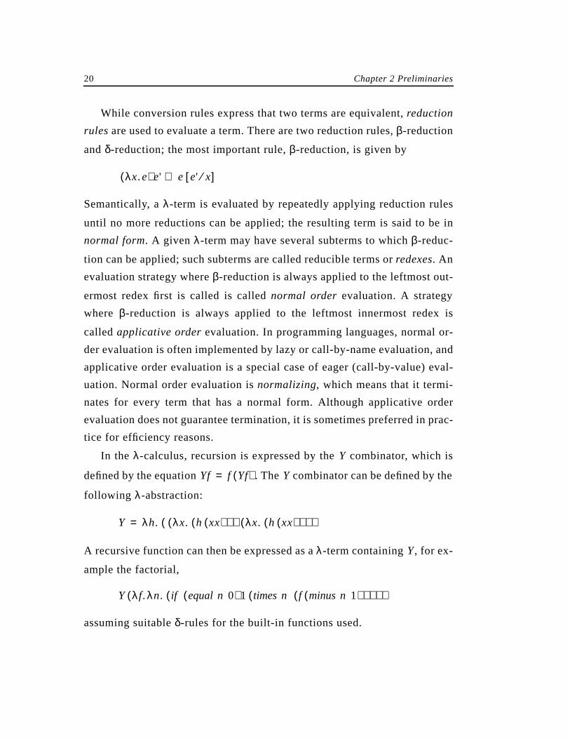
While conversion rules express that two terms are equivalent,reduction
rules are used to evaluate a term. There are two reduction rules,β-reduction
andδ-reduction; the most important rule,β-reduction, is given by
Semantically, a λ-term is evaluated by repeatedly applying reduction rules
until no more reductions can be applied; the resulting term is said to be in
normal form. A given λ-term may have several subterms to whichβ-reduc-
tion can be applied; such subterms are called reducible terms orredexes. An
evaluation strategy whereβ-reduction is always applied to the leftmost out-
ermost redex first is called is callednormal order evaluation. A strategy
where β-reduction is always applied to the leftmost innermost redex is
calledapplicative order evaluation. In programming languages, normal or-
der evaluation is often implemented by lazy or call-by-name evaluation, and
applicative order evaluation is a special case of eager (call-by-value) eval-
uation. Normal order evaluation isnormalizing, which means that it termi-
nates for every term that has a normal form. Although applicative order
evaluation does not guarantee termination, it is sometimes preferred in prac-
tice for efficiency reasons.
In the λ-calculus, recursion is expressed by the combinator, which is
defined by the equation . The combinator can be defined by the
following λ-abstraction:
A recursive function can then be expressed as aλ-term containing , for ex-
ample the factorial,
assuming suitableδ-rules for the built-in functions used.
λx.e( ) e' e e' x⁄[ ]⇒
Y
Yf f Yf( )= Y
Y λh. λx. h xx( )( )( ) λx. h xx( )( )( )( )=
Y
Y λf.λn. if equal n 0( ) 1 times n f minus n1( )( )( )( )( )
Section 2.2 The Lambda Calculus, Polymorphism, and Existential Quantification 21
2.2.2 The Simply Typedλ-Calculus
Typed λ-calculi are like the untypedλ-calculus, except that every bound
identifier is given atype. The simply typedλ-calculus describes languages
that have a notion of type. Informally, types are subsets of the set of all val-
ues that share a certain common structure, for example all integers, or all
Booleans. An important difference between typed and untyped calculi is that
typed calculi introduce the notion of (static)type correctness of a term,
which one would like to check before trying to evaluate the term. The un-
typedλ-calculus could be regarded as a typedλ-calculus in which each iden-
tifier or constant has the same type and all terms are type-correct.
An comprehensive survey of typing in programming languages is [CW85].
As an example, consider the successor function, which we could define
as
Assuming the typing , we would obtain the typing
where is the function type constructor and the tuple type constructor
used for multiple function arguments. We could then define
and the term
would be type-correct and result in . On the other hand,
would not be type-correct, since the type of is rather than .
general
succ λn : int .n 1+=
+ : int int× int→
succ : int int→
→ ×
twice λf : int int→ .λx : int . f f x( )=
twice succ( ) 4
6
twice 7
7 int int int→
22 Chapter 2 Preliminaries
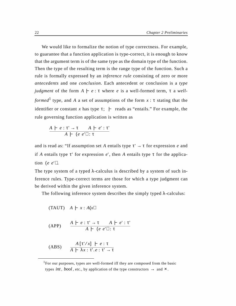
We would like to formalize the notion of type correctness. For example,
to guarantee that a function application is type-correct, it is enough to know
that the argument term is of the same type as the domain type of the function.
Then the type of the resulting term is the range type of the function. Such a
rule is formally expressed by aninference rule consisting of zero or more
antecedents and oneconclusion. Each antecedent or conclusion is atype
judgment of the form where is a well-formed term, awell-
formed1 type, and a set of assumptions of the form stating that the
identifier or constant has type ; reads as “entails.” For example, the
rule governing function application is written as
and is read as: “If assumption set entails type for expression and
if entails type for expression , then entails type for the applica-
tion .
The type system of a typedλ-calculus is described by a system of such in-
ference rules. Type-correct terms are those for which a type judgment can
be derived within the given inference system.
The following inference system describes the simply typedλ-calculus:
(TAUT)
(APP)
(ABS)
1For our purposes, types are well-formed iff they are composed from the basic
types , , etc., by application of the type constructors and .
A |− e : τ e τ
A x : τ
int bool → ×
x τ |−
A |− e : τ' τ→ A |− e' : τ'A |− e e'( ) : τ
A τ' τ→ e
A τ' e' A τ
e e'( )
A |− x : A x( )
A |− e : τ' τ→ A |− e' : τ'A |− e e'( ) : τ
A τ' x⁄[ ] |− e : τA |− λx : τ' .e : τ' τ→
Section 2.2 The Lambda Calculus, Polymorphism, and Existential Quantification 23
where stands for the assumption set extended with the assump-
tion .
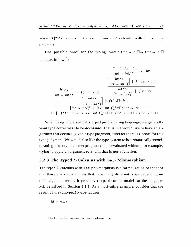
One possible proof for the typing
looks as follows1:
When designing a statically typed programming language, we generally
want type correctness to bedecidable. That is, we would like to have an al-
gorithm that decides, given a type judgment, whether there is a proof for this
type judgment. We would also like the type system to be semanticallysound,
meaning that a type-correct program can be evaluated without, for example,
trying to apply an argument to a term that is not a function.
2.2.3 The Typedλ-Calculus with let -Polymorphism
The typedλ-calculus withlet -polymorphism is a formalization of the idea
that there areλ-abstractions that have many different types depending on
their argument terms. It provides a type-theoretic model for the language
ML described in Section 2.1.1. As a motivating example, consider that the
result of the (untyped)λ-abstraction
1The horizontal bars are read in top-down order.
A τ' x⁄[ ] A
x : τ
twice : int int→( ) int int→( )→
int x⁄int int→ f⁄
|− f : int int→
int x⁄int int→ f⁄
|− x : int
int x⁄int int→ f⁄
|− f : int int→
int x⁄int int→ f⁄
|− f x : int
int x⁄int int→ f⁄
|− f f x( ) : int
int int→ f⁄[ ] |− λx : int . f f x( ) : int int→∅ |− λf : int int→ .λx : int . f f x( )( ) : int int→( ) int int→( )→
id λx.x=
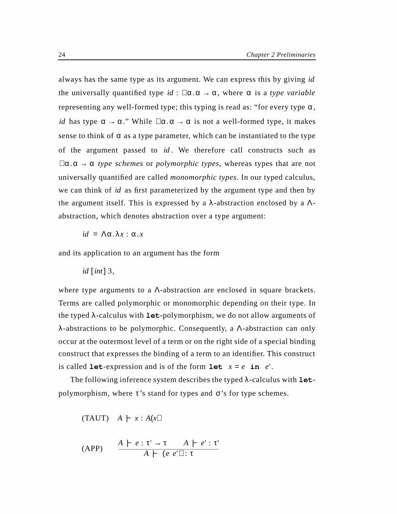
24 Chapter 2 Preliminaries
always has the same type as its argument. We can express this by giving
the universally quantified type , where is atype variable
representing any well-formed type; this typing is read as: “for every type ,
has type .” While is not a well-formed type, it makes
sense to think of as a type parameter, which can be instantiated to the type
of the argument passed to . We therefore call constructs such as
type schemes or polymorphic types, whereas types that are not
universally quantified are calledmonomorphic types. In our typed calculus,
we can think of as first parameterized by the argument type and then by
the argument itself. This is expressed by aλ-abstraction enclosed by aΛ-
abstraction, which denotes abstraction over a type argument:
and its application to an argument has the form
,
where type arguments to aΛ-abstraction are enclosed in square brackets.
Terms are called polymorphic or monomorphic depending on their type. In
the typedλ-calculus withlet -polymorphism, we do not allow arguments of
λ-abstractions to be polymorphic. Consequently, aΛ-abstraction can only
occur at the outermost level of a term or on the right side of a special binding
construct that expresses the binding of a term to an identifier. This construct
is calledlet -expression and is of the form .
The following inference system describes the typed λ-calculus withlet -
polymorphism, where ’s stand for types and ’s for type schemes.
(TAUT)
(APP)
id
id : α.∀ α α→ α
α
id α α→ α.∀ α α→
α
id
α.∀ α α→
id
id Λα.λx : α.x=
id int[ ] 3
let x e= in e'
τ σ
A |− x : A x( )
A |− e : τ' τ→ A |− e' : τ'A |− e e'( ) : τ
Section 2.2 The Lambda Calculus, Polymorphism, and Existential Quantification 25
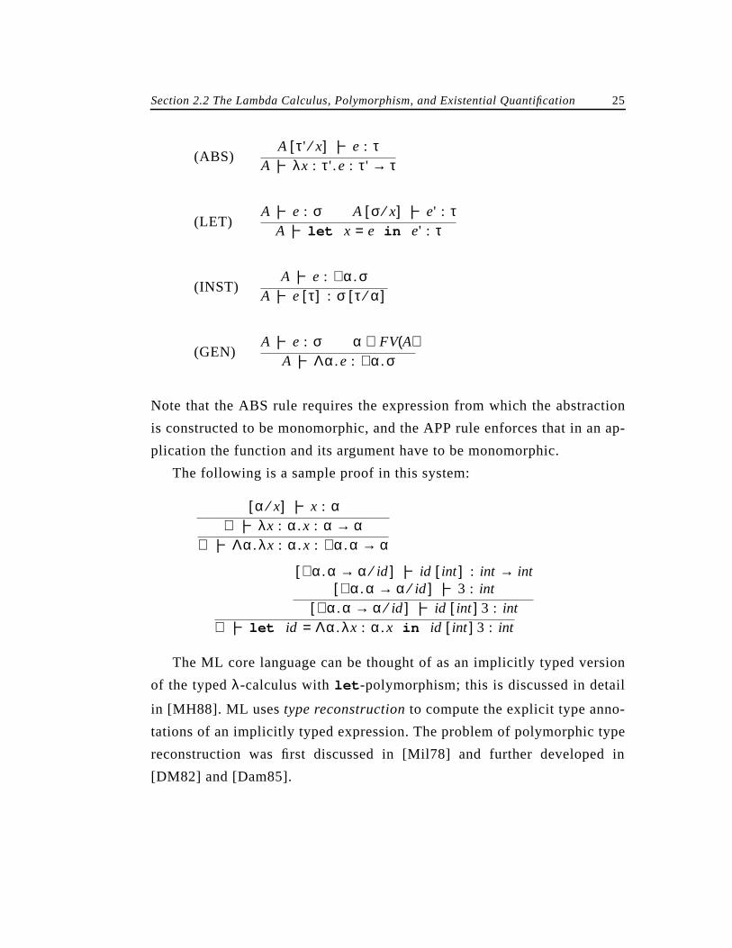
(ABS)
(LET)
(INST)
(GEN)
Note that the ABS rule requires the expression from which the abstraction
is constructed to be monomorphic, and the APP rule enforces that in an ap-
plication the function and its argument have to be monomorphic.
The following is a sample proof in this system:
The ML core language can be thought of as an implicitly typed version
of the typedλ-calculus withlet -polymorphism; this is discussed in detail
in [MH88]. ML usestype reconstruction to compute the explicit type anno-
tations of an implicitly typed expression. The problem of polymorphic type
reconstruction was first discussed in [Mil78] and further developed in
[DM82] and [Dam85].
A τ' x⁄[ ] |− e : τA |− λx : τ' .e : τ' τ→
A |− e : σ A σ x⁄[ ] |− e' : τA |− let x e= in e' : τ
A |− e : α.∀ σA |− e τ[ ] : σ τ α⁄[ ]
A |− e : σ α FV A( )∉A |− Λα.e : α.∀ σ
α x⁄[ ] |− x : α∅ |− λx : α.x : α α→
∅ |− Λα.λx : α.x : α.∀ α α→
α.∀ α α→ id⁄[ ] |− id int[ ] : int int→α.∀ α α→ id⁄[ ] |− 3 : int
α.∀ α α→ id⁄[ ] |− id int[ ] 3 : int∅ |− let id Λα.λx : α.x= in id int[ ] 3 : int
26 Chapter 2 Preliminaries
2.2.4 Higher-Order Typed λ-Calculi
A considerable amount of research has focused on the second-order typedλ-
calculus and higher-order systems [REFS]. Since all languages presented in
this dissertation are extensions of the typedλ-calculus withlet -polymor-
phism, we do not further discuss higher-order calculi here.
2.2.5 Existential Quantification
Existentially quantified types, or in short, existential types, are a type-theo-
retic formalization of the concept of abstract data types, which are featured
in different forms by various programming languages.
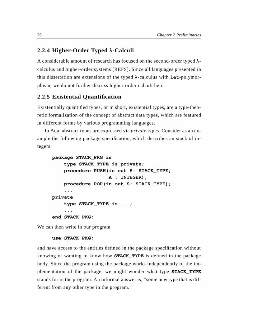
In Ada, abstract types are expressed viaprivate types. Consider as an ex-
ample the following package specification, which describes an stack of in-
tegers:
package STACK_PKG is
type STACK_TYPE is private;
procedure PUSH(in out S: STACK_TYPE;
A : INTEGER);
procedure POP(in out S: STACK_TYPE);
...
private
type STACK_TYPE is ...;
...
end STACK_PKG;
We can then write in our program
use STACK_PKG;
and have access to the entities defined in the package specification without
knowing or wanting to know howSTACK_TYPE is defined in the package
body. Since the program using the package works independently of the im-
plementation of the package, we might wonder what typeSTACK_TYPE
stands for in the program. An informal answer is, “some new type that is dif-
ferent from any other type in the program.”
Section 2.3 Type Reconstruction 27
Existential quantification is a formalization of the notion of abstract
types; it is described in [CW85] and further explored in [MP88]. By stating
that an expression has existential type , we mean that for some fixed,
unknown type , has type . can thus be viewed as a pair consist-
ing of a type component and a value component of type . The com-
ponents are accessed through anelimination construct of the form
In , the type stands for the hidden representation type of , such that
can be used in with type . To guarantee static typing, the type of
must not contain .
Values of existential type are created using the construct
where may occur free in . The type of this expression is , and at his
point we no longer know that the expression we packed originally had type
.
A different formulation of existential quantification called thedot nota-
tion, closer to actual programming languages, is described in [CL90].
2.3 Type Reconstruction
In this section, we describe the Damas-Milner approach to type reconstruc-
tion in ML [Mil78] [DM82] [Dam85] and its application to type reconstruc-
tion in Haskell [NS91].
2.3.1 Type Reconstruction for ML
Before we present the type inference system and the type reconstruction al-
gorithm for the ML core, we need to define the following terms:
• A substitution is a finite mapping from type variables to types. It is of-
e α.∃ τ
τ e τ τ α⁄[ ] e
τ τ τ α⁄[ ]
open e as t x,⟨ ⟩ in e'
e' t e x
e' τ t α⁄[ ]
e' t
pack α τ= e : τ,⟨ ⟩
α τ α.∃ τ
τ τ α⁄[ ]
28 Chapter 2 Preliminaries
ten written in the form and applied as a postfix op-
erator; it can also be given a name, for example, , and applied as pre-
fix operator. If is a type scheme, then is the type
scheme obtained from by replacing each free occurrence of in
by , renaming the bound variables of if necessary. Let denote
the identity substitution .
• Type is aprincipal type of expression under assumption set if
and whenever then there is a substitution such
that ,
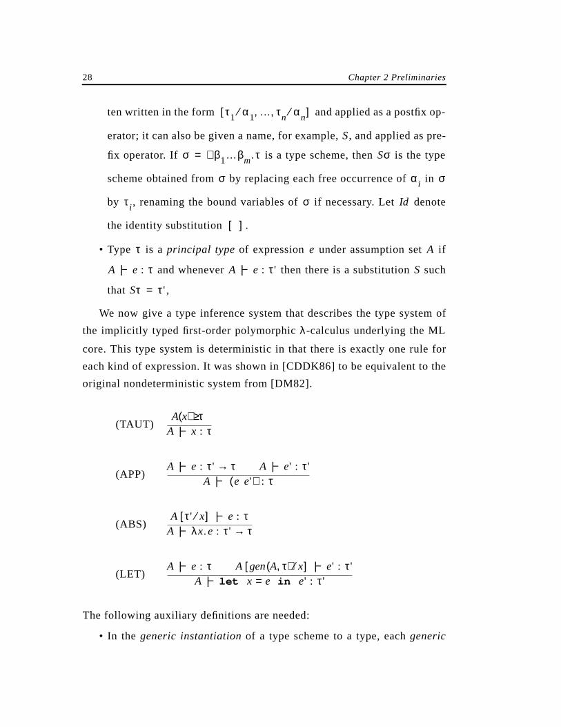
We now give a type inference system that describes the type system of
the implicitly typed first-order polymorphicλ-calculus underlying the ML
core. This type system is deterministic in that there is exactly one rule for
each kind of expression. It was shown in [CDDK86] to be equivalent to the
original nondeterministic system from [DM82].
(TAUT)
(APP)
(ABS)
(LET)
The following auxiliary definitions are needed:
• In the generic instantiation of a type scheme to a type, eachgeneric
τ1 α1⁄ … τn αn⁄, ,[ ]
S
σ β1…βm.∀ τ= Sσ
σ αi σ
τi σ Id
[ ]
τ e A
A |− e : τ A |− e : τ' S
Sτ τ'=
A x( ) τ≥A |− x : τ
A |− e : τ' τ→ A |− e' : τ'A |− e e'( ) : τ
A τ' x⁄[ ] |− e : τA |− λx.e : τ' τ→
A |− e : τ A gen A τ,( ) x⁄[ ] |− e' : τ'A |− let x e= in e' : τ'
Section 2.3 Type Reconstruction 29
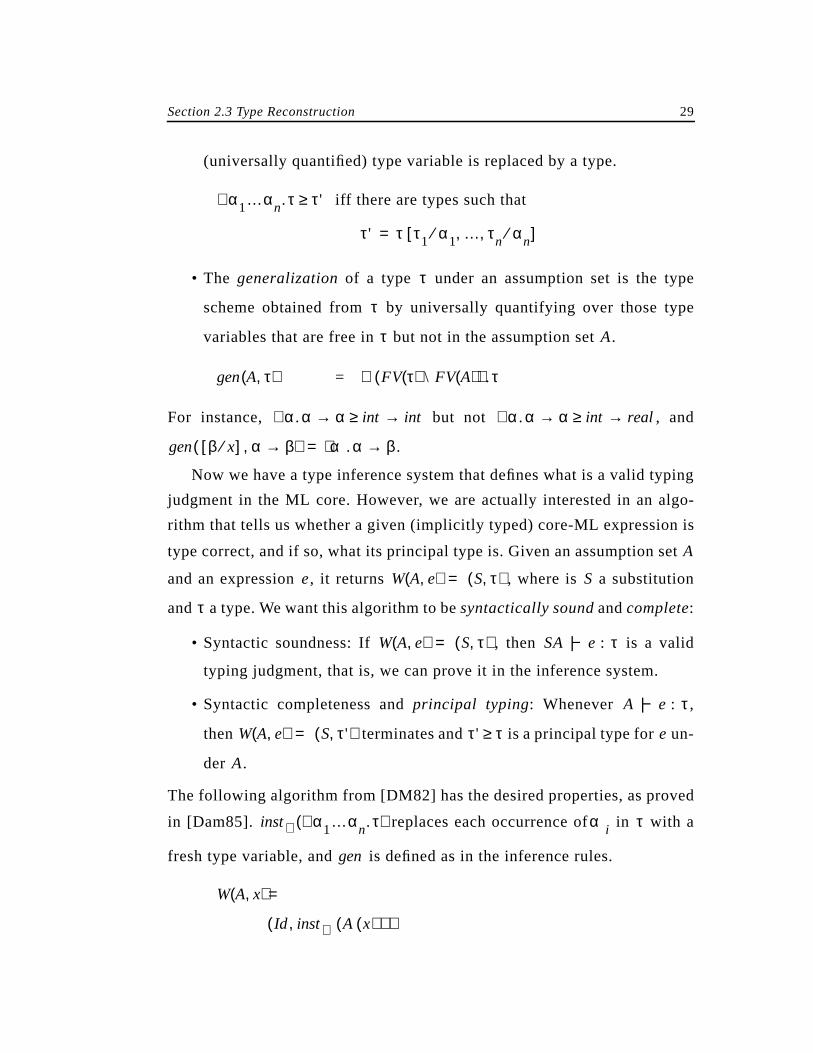
(universally quantified) type variable is replaced by a type.
iff there are types such that
• The generalization of a type under an assumption set is the type
scheme obtained from by universally quantifying over those type
variables that are free in but not in the assumption set .
=
For instance, but not , and
.
Now we have a type inference system that defines what is a valid typing
judgment in the ML core. However, we are actually interested in an algo-
rithm that tells us whether a given (implicitly typed) core-ML expression is
type correct, and if so, what its principal type is. Given an assumption set
and an expression , it returns , where is a substitution
and a type. We want this algorithm to besyntactically soundand complete:
• Syntactic soundness: If , then is a valid
typing judgment, that is, we can prove it in the inference system.
• Syntactic completeness andprincipal typing: Whenever ,
then terminates and is a principal type for un-
der .
The following algorithm from [DM82] has the desired properties, as proved
in [Dam85]. replaces each occurrence of in with a
fresh type variable, and is defined as in the inference rules.
α1…αn.∀ τ τ'≥
τ' τ τ1 α1⁄ … τn αn⁄, ,[ ]=
τ
τ
τ A
gen A τ,( ) FV τ( ) \ FV A( )( ) .∀ τ
α.∀ α α→ int int→≥ α.∀ α α→ int real→≥
gen β x⁄[ ] α β→,( ) α.∀ α β→=
A
e W A e,( ) S τ,( )= S
τ
W A e,( ) S τ,( )= SA |− e : τ
A |− e : τ
W A e,( ) S τ',( )= τ' τ≥ e
A
inst∀ α1…αn∀ .τ( ) αi τ
gen
W A x,( ) =
Id inst∀ A x( )( ),( )
30 Chapter 2 Preliminaries
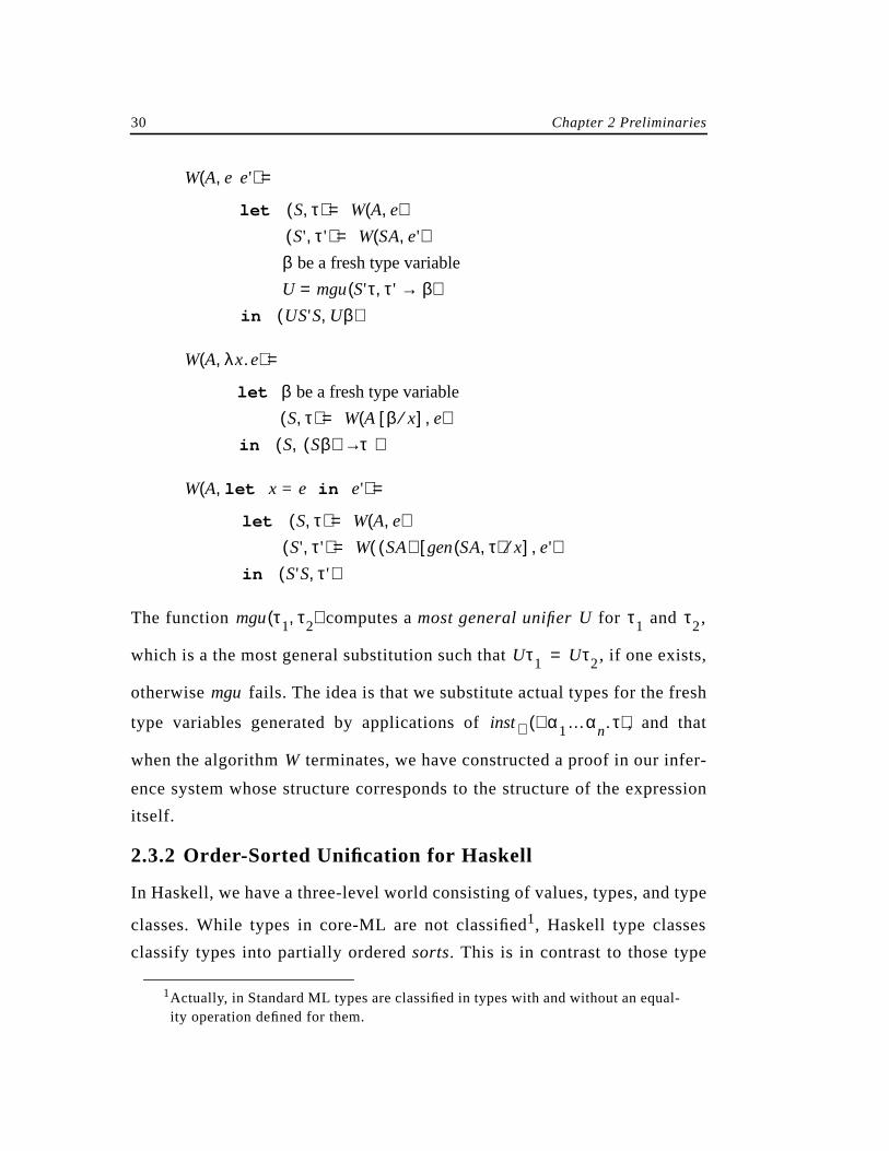
The function computes amost general unifier for and ,
which is a the most general substitution such that , if one exists,
otherwise fails. The idea is that we substitute actual types for the fresh
type variables generated by applications of , and that
when the algorithm terminates, we have constructed a proof in our infer-
ence system whose structure corresponds to the structure of the expression
itself.
2.3.2 Order-Sorted Unification for Haskell
In Haskell, we have a three-level world consisting of values, types, and type
classes. While types in core-ML are not classified1, Haskell type classes
classify types into partially orderedsorts. This is in contrast to those type
1Actually, in Standard ML types are classified in types with and without an equal-ity operation defined for them.
W A e e',( ) =
let S τ,( ) = W A e,( )S' τ',( ) = W SA e',( )
β be a fresh type variable
U = mgu S'τ τ' β→,( )in US'S Uβ,( )
W A λx.e,( ) =
let β be a fresh type variable
S τ,( ) = W A β x⁄[ ] e,( )in S Sβ( ) τ→,( )
W A let x = e in e',( ) =
let S τ,( ) = W A e,( )S' τ',( ) = W SA( ) gen SAτ,( ) x⁄[ ] e',( )
in S'S τ',( )
mgu τ1 τ2,( ) U τ1 τ2
Uτ1 Uτ2=
mgu
inst∀ α1…αn∀ .τ( )
W
Section 2.3 Type Reconstruction 31
systems where types themselves are partially ordered, for example the one
of OBJ [FGJM85].Order-sorted unification [MGS89] can be used to obtain
a type reconstruction algorithm in an order-sorted type system such as
Haskell’s; this is described in [NS91].
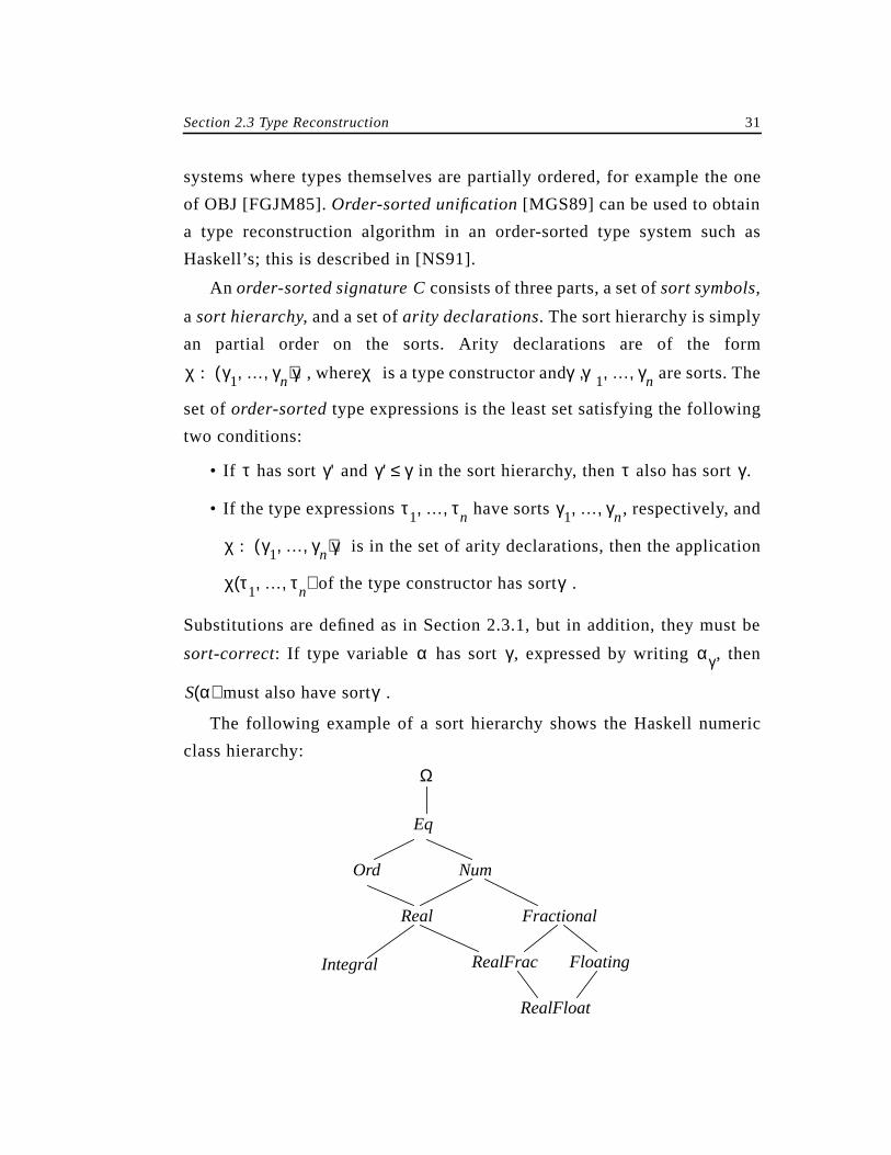
An order-sorted signature consists of three parts, a set ofsort symbols,
a sort hierarchy, and a set ofarity declarations. The sort hierarchy is simply
an partial order on the sorts. Arity declarations are of the form
, where is a type constructor and are sorts. The
set oforder-sorted type expressions is the least set satisfying the following
two conditions:
• If has sort and in the sort hierarchy, then also has sort .
• If the type expressions have sorts , respectively, and
is in the set of arity declarations, then the application
of the type constructor has sort .
Substitutions are defined as in Section 2.3.1, but in addition, they must be
sort-correct: If type variable has sort , expressed by writing , then
must also have sort .
The following example of a sort hierarchy shows the Haskell numeric
class hierarchy:
C
χ : γ1 … γn, ,( ) γ χ γ γ1 … γn, , ,
τ γ' γ' γ≤ τ γ
τ1 … τn, , γ1 … γn, ,
χ : γ1 … γn, ,( ) γ
χ τ1 … τn, ,( ) γ
α γ αγ
S α( ) γ
Ω
Eq
Ord Num
Real
Integral RealFrac
Fractional
Floating
RealFloat
32 Chapter 2 Preliminaries
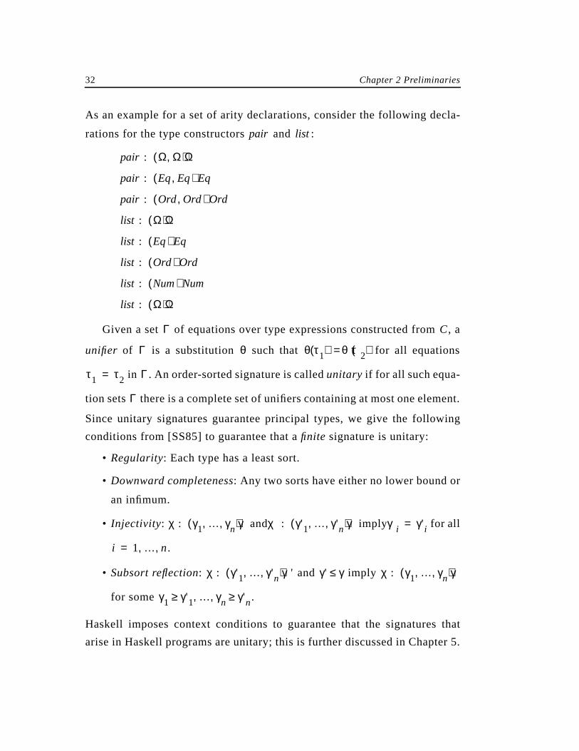
As an example for a set of arity declarations, consider the following decla-
rations for the type constructors and :
Given a set of equations over type expressions constructed from , a
unifier of is a substitution such that for all equations
in . An order-sorted signature is calledunitary if for all such equa-
tion sets there is a complete set of unifiers containing at most one element.
Since unitary signatures guarantee principal types, we give the following
conditions from [SS85] to guarantee that afinite signature is unitary:
• Regularity: Each type has a least sort.
• Downward completeness: Any two sorts have either no lower bound or
an infimum.
• Injectivity: and imply for all
.
• Subsort reflection: and imply
for some .
Haskell imposes context conditions to guarantee that the signatures that
arise in Haskell programs are unitary; this is further discussed in Chapter 5.
pair list
pair : Ω Ω,( ) Ω
pair : Eq Eq,( ) Eq
pair : Ord Ord,( ) Ord
list : Ω( ) Ω
list : Eq( ) Eq
list : Ord( ) Ord
list : Num( ) Num
list : Ω( ) Ω
Γ C
Γ θ θ τ1( ) θ τ2( )=
τ1 τ2= Γ
Γ
χ : γ1 … γn, ,( ) γ χ : γ'1 … γ'n, ,( ) γ γi γ' i=
i 1 … n, ,=
χ : γ'1 … γ'n, ,( ) γ' γ' γ≤ χ : γ1 … γn, ,( ) γ
γ1 γ'1≥ … γn γ'n≥, ,
Section 2.4 Semantics 33
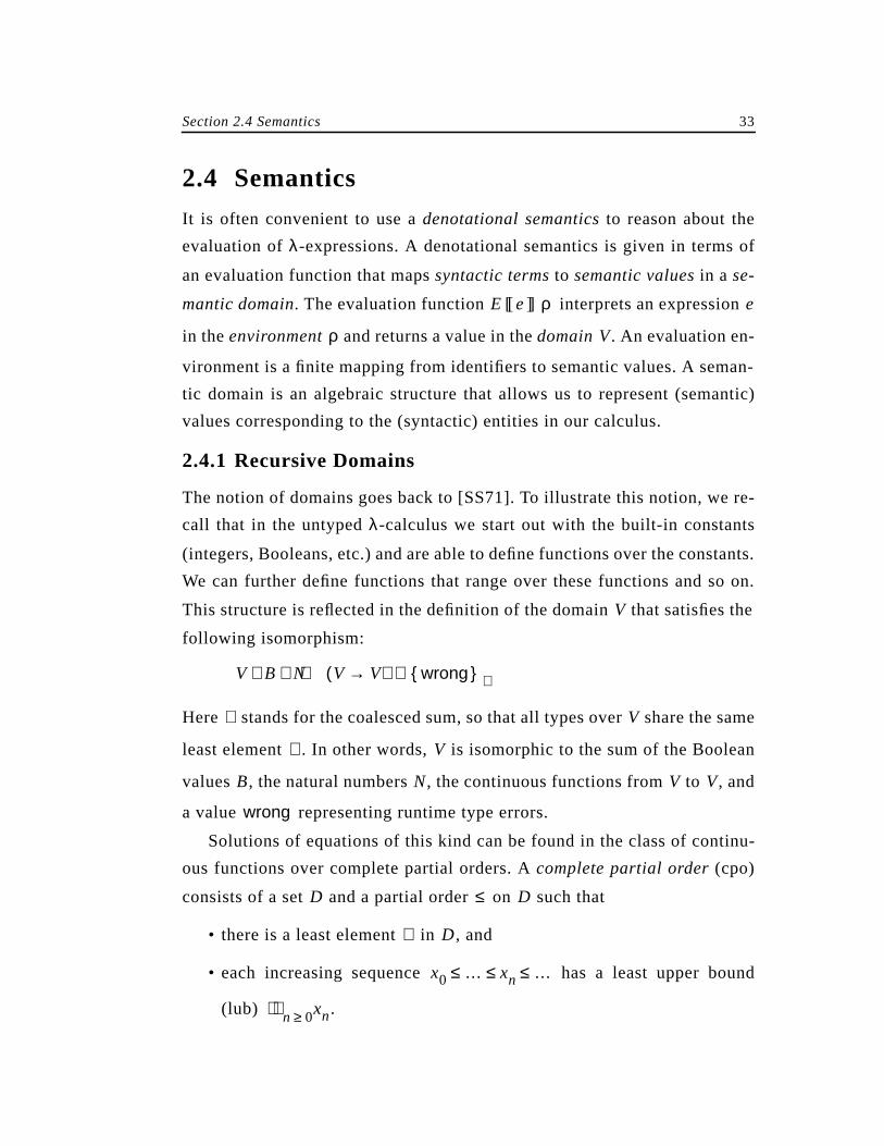
2.4 Semantics
It is often convenient to use adenotational semantics to reason about the
evaluation ofλ-expressions. A denotational semantics is given in terms of
an evaluation function that mapssyntactic terms to semantic values in a se-
mantic domain. The evaluation function interprets an expression
in theenvironment and returns a value in thedomain . An evaluation en-
vironment is a finite mapping from identifiers to semantic values. A seman-
tic domain is an algebraic structure that allows us to represent (semantic)
values corresponding to the (syntactic) entities in our calculus.
2.4.1 Recursive Domains
The notion of domains goes back to [SS71]. To illustrate this notion, we re-
call that in the untypedλ-calculus we start out with the built-in constants
(integers, Booleans, etc.) and are able to define functions over the constants.
We can further define functions that range over these functions and so on.
This structure is reflected in the definition of the domain that satisfies the
following isomorphism:
Here stands for the coalesced sum, so that all types over share the same
least element . In other words, is isomorphic to the sum of the Boolean
values , the natural numbers , the continuous functions from to , and
a value representing runtime type errors.
Solutions of equations of this kind can be found in the class of continu-
ous functions over complete partial orders. Acomplete partial order (cpo)
consists of a set and a partial order on such that
• there is a least element in , and
• each increasing sequence has a least upper bound
(lub) .
E [[ e]] ρ e
ρ V
V
V B N V V→( ) wrong ⊥++ +≅
+ V
⊥ V
B N V V
wrong
D ≤ D
⊥ D
x0 … xn …≤ ≤ ≤
n 0≥ xn
34 Chapter 2 Preliminaries
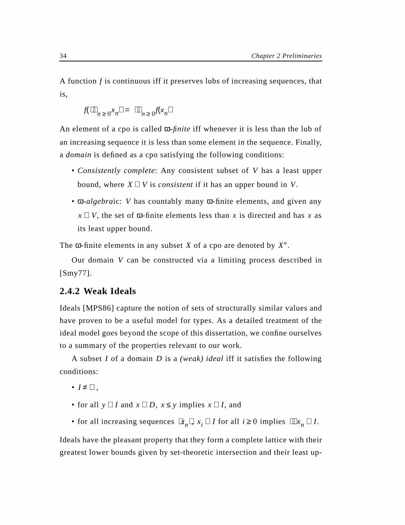
A function is continuous iff it preserves lubs of increasing sequences, that
is,
An element of a cpo is calledω-finite iff whenever it is less than the lub of
an increasing sequence it is less than some element in the sequence. Finally,
a domain is defined as a cpo satisfying the following conditions:
• Consistently complete: Any consistent subset of has a least upper
bound, where isconsistent if it has an upper bound in .
• ω-algebraic: has countably manyω-finite elements, and given any
, the set ofω-finite elements less than is directed and has as
its least upper bound.
The ω-finite elements in any subset of a cpo are denoted by .
Our domain can be constructed via a limiting process described in
[Smy77].
2.4.2 Weak Ideals
Ideals [MPS86] capture the notion of sets of structurally similar values and
have proven to be a useful model for types. As a detailed treatment of the
ideal model goes beyond the scope of this dissertation, we confine ourselves
to a summary of the properties relevant to our work.
A subset of a domain is a(weak) ideal iff it satisfies the following
conditions:
• ,
• for all and , implies , and
• for all increasing sequences , for all implies .
Ideals have the pleasant property that they form a complete lattice with their
greatest lower bounds given by set-theoretic intersection and their least up-
f
f n 0≥ xn( ) n 0≥ f xn( )=
V
X V⊆ V
V
x V∈ x x
X X°
V
I D
I ∅≠
y I∈ x D∈ x y≤ x I∈
xn⟨ ⟩ xi I∈ i 0≥ xn I∈
Section 2.4 Semantics 35
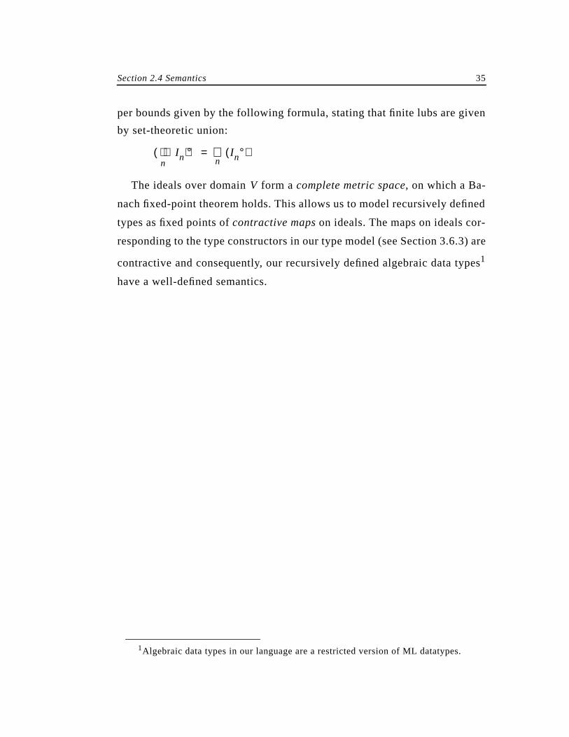
per bounds given by the following formula, stating that finite lubs are given
by set-theoretic union:
The ideals over domain form acomplete metric space, on which a Ba-
nach fixed-point theorem holds. This allows us to model recursively defined
types as fixed points ofcontractive maps on ideals. The maps on ideals cor-
responding to the type constructors in our type model (see Section 3.6.3) are
contractive and consequently, our recursively defined algebraic data types1
have a well-defined semantics.
1Algebraic data types in our language are a restricted version of ML datatypes.
n
In( ) ° In°( )n∪=
V
36
3 An Extension of ML with First-Class Abstract Types
This chapter presents a semantic extension of ML, where the component
types of a datatype may be existentially quantified. We show how datatypes
over existential types add significant flexibility to the language without even
changing ML syntax. We then describe a deterministic Damas-Milner type
inference system [DM82] [CDDK86] for this language, which leads to a
syntactically sound and complete type reconstruction algorithm. Further-
more, the type system is shown to be semantically sound with respect to a
standard denotational semantics.
3.1 Introduction
In ML, datatype declarations are of the form
datatype = of | … | of
where the ’s are value constructors and the optional prefix argument
is used for formal type parameters, which may appear free in the component
types . The types of the value constructor functions are universally quan-
tified over these type parameters, and no other type variables may appear
free in the ’s.
arg[ ] T K1 τ1 Kn τn
K arg
τi
τi
Section 3.1 Introduction 37
An example for an ML datatype declaration is
datatype ’a Mytype = mycons of ’a * (’a -> int)
Without altering the syntax of the datatype declaration, we now give a
meaning to type variables that appear free in the component types, but do
not occur in the type parameter list. We interpret such type variables as ex-
istentially quantified.
For example,
datatype Key = key of ’a * (’a -> int)
describes a datatype with one value constructor whose arguments are pairs
of a value of type’a and a function from type’a to int . The question is
what we can say about’a . The answer is, nothing, except that the value is
of the same type’a as the function domain. To illustrate this further, the
type of the expression
key(3,fn x => 5)
is Key, as is the type of the expression
key([1,2,3],length)
wherelength is the built-in function on lists. Note that no argument types
appear in the result type of the expression. On the other hand,
key(3,length)
is not type-correct, since the type of3 is different from the domain type of
length .
We recognize thatKey is an abstract type comprised by a value of some
type and an operation on that type yielding anint . It is important to note
that values of typeKey are first-class; they may be created dynamically and
passed around freely as function parameters. The two different values of
type Key in the previous examples may be viewed as two different imple-
mentations of the same abstract type.
38 Chapter 3 An Extension of ML with First-Class Abstract Types
Besides constructing values of datatypes with existential component
types, we can decompose them using thelet construct. We impose the re-
striction that no type variable that is existentially quantified in alet expres-
sion appears in the result type of this expression or in the type of a global
identifier. Analogous restrictions hold for the correspondingopen andab-
stype constructs described in [CW85] [MP88].
For example, assumingx is of typeKey, then
let val key(v,f) = x in
f v
end
has a well-defined meaning, namely theint result of f applied tov. We
know that this application is type-safe because the pattern matching suc-
ceeds, sincex was constructed using constructorkey , and at that time it was
enforced thatf can safely be applied tov. On the other hand,
let val key(v,f) = x in
v
end
is not type-correct, since we do not know the type ofv statically and, con-
sequently, cannot assign a type to the whole expression.
Our extension to ML allows us to deal with existential types as described
in [CW85] [MP88], with the further improvement that decomposed values
of existential type arelet -bound and may be instantiated polymorphically.
This is illustrated by the following example,
datatype ’a t = k of (’a -> ’b) * (’b -> int)
let val k(f1,f2) = k(fn x => x,fn x => 3) in
(f2(f1 7),f2(f1 true))
end
which results in(3,3) . In most previous work, the value on the right-hand
side of the binding would have to be bound and decomposed twice.
Section 3.2 Some Motivating Examples 39
3.2 Some Motivating Examples
3.2.1 Minimum over a Heterogeneous List
Extending on the previous example, we first show how we construct heter-
ogeneous lists over different implementations of the same abstract type and
define functions that operate uniformly on such heterogeneous lists. A het-
erogeneous list of values of typeKey could be defined as follows:
val hetlist = [key(3,fn x => x),
key([1,2,3,4],length),
key(7,fn x => 0),
key(true,fn x => if x then 1 else 0),
key(12,fn x => 3)]
The type ofhetlist is Key list ; it is a homogeneous list of elements each
of which could be a different implementation of typeKey. We define the
functionmin , which finds the minimum of a list ofKey ’s with respect to the
integer value obtained by applying the second component (the function) to
the first component (the value).
fun min [x] = x
| min ((key(v1,f1))::xs) =
let val key(v2,f2) = min xs in
if f1 v1 <= f2 v2 then
key(v1,f1)
else
key(v2,f2)
end
Thenmin hetlist returnskey(7,fn x => 0) , the third element of the
list.
3.2.2 Stacks Parametrized by Element Type
The preceding example involves a datatype with existential types but with-
out polymorphic type parameters. As a practical example involving both ex-
40 Chapter 3 An Extension of ML with First-Class Abstract Types
istential and universal quantification, we show an abstract stack parame-
trized by element type.
datatype ’a Stack =
stack of value : ’b,
empty : ’b,
push : ’a -> ’b -> ’b
pop : ’b -> ’b
top : ’b -> ’a,
isempty : ’b -> bool
An on-the-fly implementation of anint Stack in terms of the built-in type
list can be given as
stackvalue = [1,2,3], empty = [],
push = fn x => fn xs => x :: xs,
pop = tl, top = hd, isempty = null
An alternative implementation ofStack could be given, among others,
based on arrays. We provide a constructor for each implementation:
fun makeListStack xs = stackvalue = xs, empty = [],
push = fn x => fn xs => x :: xs, pop = tl,
top = hd, isempty = null
fun makeArrayStack xs = stack...
To achieve dynamic dispatching, one can provide stack operations that work
uniformly across implementations. These “outer” wrappers work by opening
the stack, applying the intended “inner” operations, and encapsulating the
stack again, for example:
fun push a (stackvalue = v, push = pu, empty = e,
pop = po, top = t, isempty = i) =
stackvalue = pu a v, push = pu,
empty = e, pop = po,
top = t, isempty = i
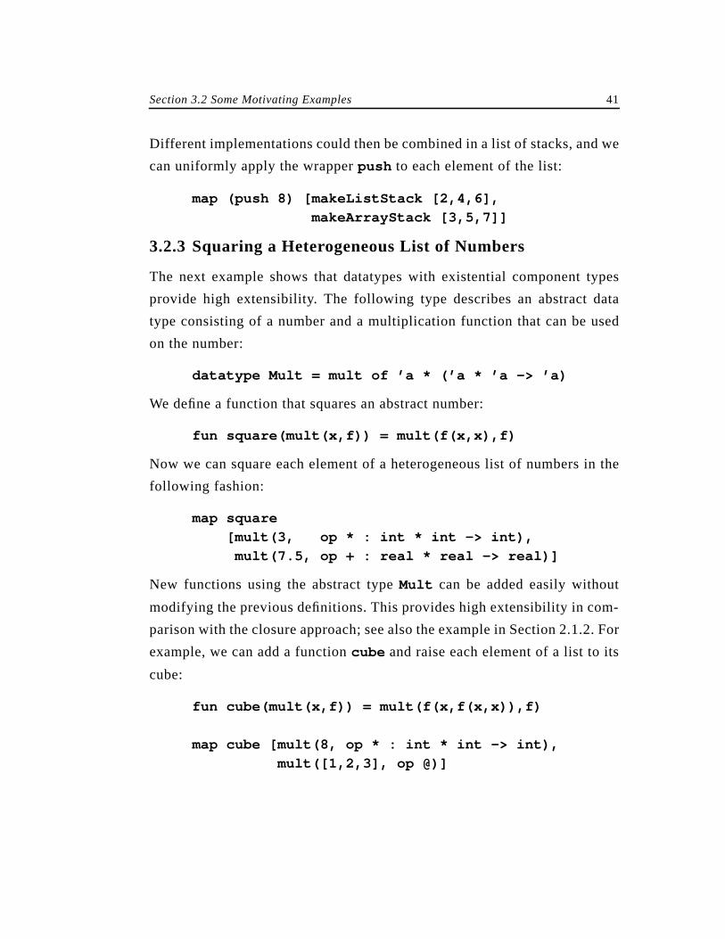
Section 3.2 Some Motivating Examples 41
Different implementations could then be combined in a list of stacks, and we
can uniformly apply the wrapperpush to each element of the list:
map (push 8) [makeListStack [2,4,6],
makeArrayStack [3,5,7]]
3.2.3 Squaring a Heterogeneous List of Numbers
The next example shows that datatypes with existential component types
provide high extensibility. The following type describes an abstract data
type consisting of a number and a multiplication function that can be used
on the number:
datatype Mult = mult of ’a * (’a * ’a -> ’a)
We define a function that squares an abstract number:
fun square(mult(x,f)) = mult(f(x,x),f)
Now we can square each element of a heterogeneous list of numbers in the
following fashion:
map square
[mult(3, o p * : int * int -> int),
mult(7.5, o p + : real * real -> real)]
New functions using the abstract typeMult can be added easily without
modifying the previous definitions. This provides high extensibility in com-
parison with the closure approach; see also the example in Section 2.1.2. For
example, we can add a functioncube and raise each element of a list to its
cube:
fun cube(mult(x,f)) = mult(f(x,f(x,x)),f)
map cube [mult(8, o p * : int * int -> int),
mult([1,2,3], op @)]
42 Chapter 3 An Extension of ML with First-Class Abstract Types
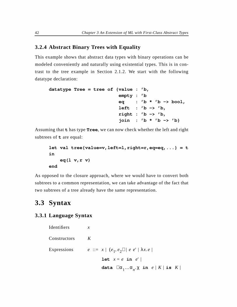
3.2.4 Abstract Binary Trees with Equality
This example shows that abstract data types with binary operations can be
modeled conveniently and naturally using existential types. This is in con-
trast to the tree example in Section 2.1.2. We start with the following
datatype declaration:
datatype Tree = tree of value : ’b,
empty : ’b
eq : ’b * ’b -> bool,
left : ’b -> ’b,
right : ’b -> ’b,
join : ’b * ’b -> ’b
Assuming thatt has typeTree , we can now check whether the left and right
subtrees oft are equal:
let val treevalue=v,left=l,right=r,eq=eq,... = t
in
eq(l v,r v)
end
As opposed to the closure approach, where we would have to convert both
subtrees to a common representation, we can take advantage of the fact that
two subtrees of a tree already have the same representation.
3.3 Syntax
3.3.1 Language Syntax
Identifiers
Constructors
Expressions ::= | | | |
|
| | |
x
K
e x e1 e2,( ) e e' λx.e
let x = e in e'
data α1…αn.∀ χ in e K is K
Section 3.3 Syntax 43
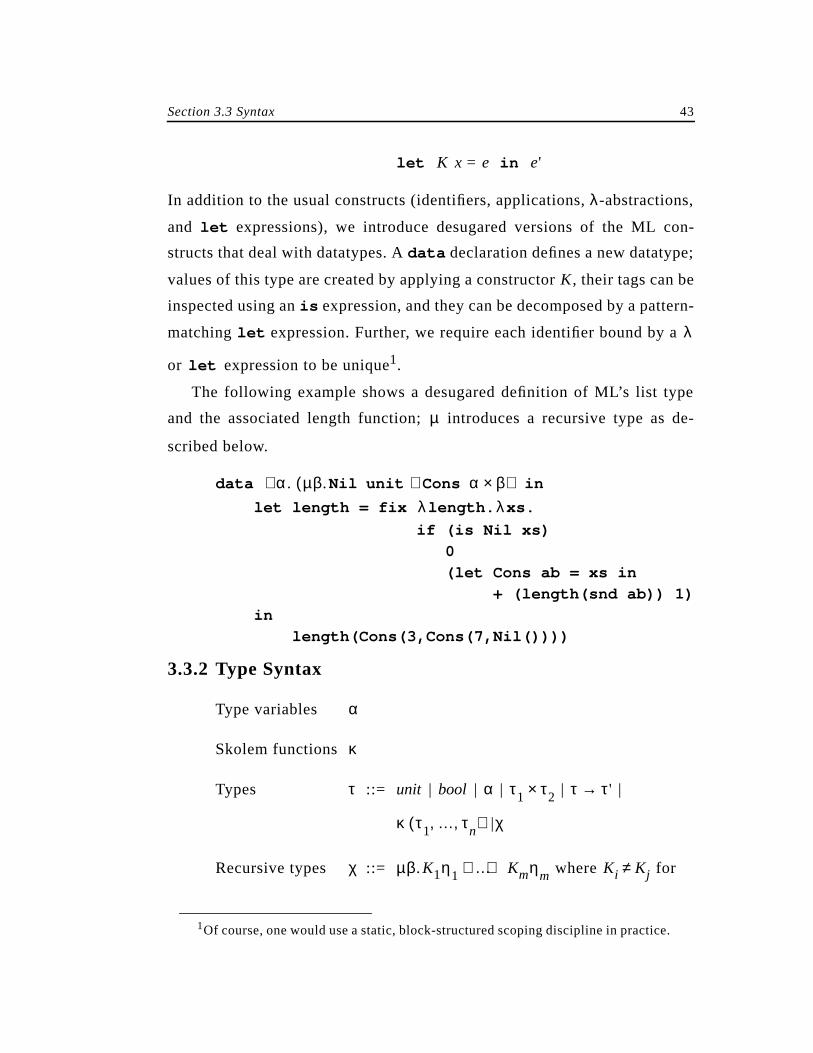
In addition to the usual constructs (identifiers, applications,λ-abstractions,
and let expressions), we introduce desugared versions of the ML con-
structs that deal with datatypes. Adata declaration defines a new datatype;
values of this type are created by applying a constructor , their tags can be
inspected using anis expression, and they can be decomposed by a pattern-
matchinglet expression. Further, we require each identifier bound by a
or expression to be unique1.
The following example shows a desugared definition of ML’s list type
and the associated length function; introduces a recursive type as de-
scribed below.
data in
let length = fix length. xs.
if (is Nil xs)
0
(let Cons ab = xs in
+ (length(snd ab)) 1)
in
length(Cons(3,Cons(7,Nil())))
3.3.2 Type Syntax
Type variables
Skolem functions
Types ::= | | | | |
|
Recursive types ::= where for
1Of course, one would use a static, block-structured scoping discipline in practice.
let K x = e in e'
K
λ
let
µ
α.∀ µβ.Nil unit Cons α β×+( )λ λ
α
κ
τ unit bool α τ1 τ2× τ τ'→
κ τ1 … τn, ,( ) χ
χ µβ.K1η1 … Kmηm+ + Ki Kj≠
44 Chapter 3 An Extension of ML with First-Class Abstract Types
Existential types ::= |
Type schemes ::= |
Assumptions ::= |
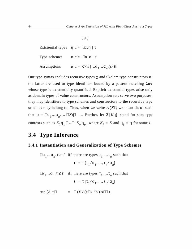
Our type syntax includes recursive types and Skolem type constructors ;
the latter are used to type identifiers bound by a pattern-matchinglet
whose type is existentially quantified. Explicit existential types arise only
as domain types of value constructors. Assumption sets serve two purposes:
they map identifiers to type schemes and constructors to the recursive type
schemes they belong to. Thus, when we write , we mean the such
that . Further, let stand for sum type
contexts such as , where and for some .
3.4 Type Inference
3.4.1 Instantiation and Generalization of Type Schemes
iff there are types such that
iff there are types such that
=
i j≠
η α.η∃ τ
σ α.σ∀ τ
a σ x⁄ α1…αn.∀ χ K⁄
χ κ
A K( ) σ
σ α1…αn.∀ … Kη …+ += Σ Kη[ ]
K1η1 … Kmηm+ + Ki K= ηi η= i
α1…αn.τ∀ τ'≥ τ1 …τn,
τ' τ τ1 α1⁄ … τn αn⁄, ,[ ]=
α1…αn.τ∃ τ'≤ τ1 …τn,
τ' τ τ1 α1⁄ … τn αn⁄, ,[ ]=
gen A τ,( ) FV τ( ) \ FV A( )( ) .τ∀
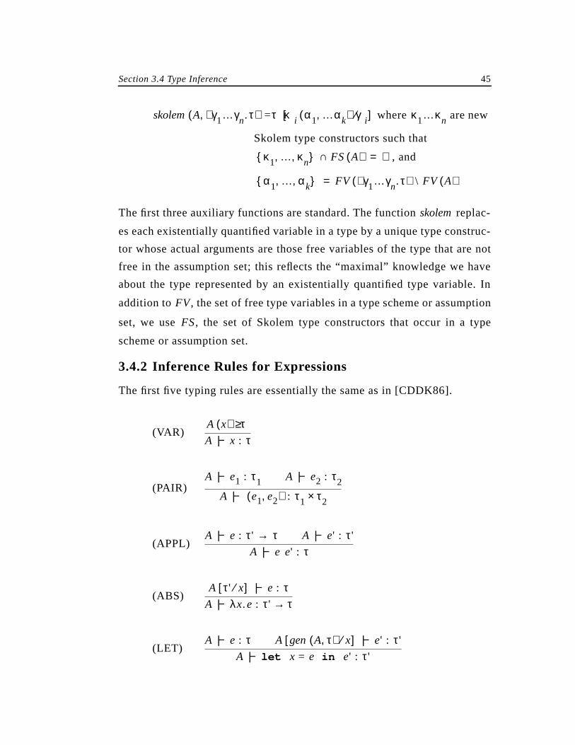
Section 3.4 Type Inference 45
= where are new
Skolem type constructors such that
, and
The first three auxiliary functions are standard. The function replac-
es each existentially quantified variable in a type by a unique type construc-
tor whose actual arguments are those free variables of the type that are not
free in the assumption set; this reflects the “maximal” knowledge we have
about the type represented by an existentially quantified type variable. In
addition to , the set of free type variables in a type scheme or assumption
set, we use , the set of Skolem type constructors that occur in a type
scheme or assumption set.
3.4.2 Inference Rules for Expressions
The first five typing rules are essentially the same as in [CDDK86].
(VAR)
(PAIR)
(APPL)
(ABS)
(LET)
skolem A γ1…γn.τ∃,( ) τ κi α1 …αk,( ) γi⁄[ ] κ1…κn
κ1 … κn, , FS A( )∩ ∅=
α1 … αk, , FV γ1…γn.τ∃( ) \ FV A( )=
skolem
FV
FS
A x( ) τ≥A |− x : τ
A |− e1 : τ1 A |− e2 : τ2
A |− e1 e2,( ) : τ1 τ2×
A |− e : τ' → τ A |− e' : τ'
A |− e e' : τ
A τ' x⁄[ ] |− e : τA |− λx.e : τ' τ→
A |− e : τ A gen A τ,( ) x⁄[ ] |− e' : τ'
A |− let x = e in e' : τ'
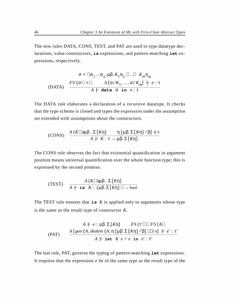
46 Chapter 3 An Extension of ML with First-Class Abstract Types
The new rules DATA, CONS, TEST, and PAT are used to type datatype dec-
larations, value constructors,is expressions, and pattern-matchinglet ex-
pressions, respectively.
(DATA)
The DATA rule elaborates a declaration of a recursive datatype. It checks
that the type scheme is closed and types the expression under the assumption
set extended with assumptions about the constructors.
(CONS)
The CONS rule observes the fact that existential quantification in argument
position means universal quantification over the whole function type; this is
expressed by the second premise.
(TEST)
The TEST rule ensures that is applied only to arguments whose type
is the same as the result type of constructor .
(PAT)
The last rule, PAT, governs the typing of pattern-matchinglet expressions.
It requires that the expression be of the same type as the result type of the
σ α1…αn.∀ µβ.K1η1 … Kmηm+ +=
FV σ( ) ∅= A σ K1⁄ … σ Km⁄, ,[ ] |− e : τA |− data σ in e : τ
A K( ) µβ.Σ Kη[ ]≥ η µβ.Σ Kη[ ] β⁄[ ] τ≤A |− K : τ µβ.Σ Kη[ ]→
A K( ) µβ.Σ Kη[ ]≥A |− is K : µβ.Σ Kη[ ]( ) bool→
is K
K
A |− e : µβ.Σ Kη[ ] FS τ'( ) FS A( )⊆A gen A skolem Aη µβ.Σ Kη[ ] β⁄[ ],( ),( ) x⁄[ ] |− e' : τ'
A |− let K x = e in e' : τ'
e
Section 3.4 Type Inference 47
constructor . The body is typed under the assumption set extended with
an assumption about the bound identifier . By definition of the function
, the new Skolem type constructors do not appear in ; this ensures
that they do not appear in the type of any identifier free in other than .
It is also guaranteed that the Skolem constructors do not appear in the result
type .
3.4.3 Relation to the ML Type Inference System
We compare our system with Mini-ML’, an extension of Mini-ML with re-
cursive datatypes, but without existential quantification. Mini-ML’ has the
same syntax as our language. The type inference system of Mini-ML’ con-
sists of the rules VAR, PAIR, APPL, ABS, and LET, and the following mod-
ified versions of the remaining rules1:
(DATA’)
(CONS’)
(TEST’)
(PAT’)
1Theoretically, it is sufficient to modify only the DATA rule to preclude that exis-tential quantifiers arise in the inference system; however, it is more illustrativeto present modified versions of the CONS, TEST, and PAT rules as well.
K e'
x
skolem A
e' x
τ'
σ α1…αn.∀ µβ.K1τ1 … Kmτm+ +=
FV σ( ) ∅= A σ K1⁄ … σ Km⁄, ,[ ] |− e : τA |− data σ in e : τ
A K( ) µβ.Σ Kτ[ ]≥A |− K : τ µβ.Σ Kτ[ ]→
A K( ) µβ.Σ Kτ[ ]≥A |− is K : µβ.Σ Kτ[ ]( ) bool→
A |− e : µβ.Σ Kτ[ ]A gen A τ µβ.Σ Kτ[ ] β⁄[ ],( ) x⁄[ ] |− e' : τ'
A |− let K x = e in e' : τ'
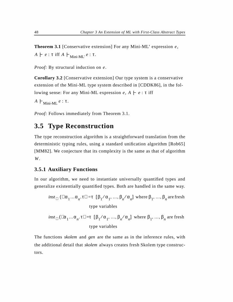
48 Chapter 3 An Extension of ML with First-Class Abstract Types
Theorem 3.1[Conservative extension] For any Mini-ML’ expression ,
iff .
Proof: By structural induction on .
Corollary 3.2 [Conservative extension] Our type system is a conservative
extension of the Mini-ML type system described in [CDDK86], in the fol-
lowing sense: For any Mini-ML expression , iff
.
Proof: Follows immediately from Theorem 3.1.
3.5 Type Reconstruction
The type reconstruction algorithm is a straightforward translation from the
deterministic typing rules, using a standard unification algorithm [Rob65]
[MM82]. We conjecture that its complexity is the same as that of algorithm
.
3.5.1 Auxiliary Functions
In our algorithm, we need to instantiate universally quantified types and
generalize existentially quantified types. Both are handled in the same way.
= where are fresh
type variables
= where are fresh
type variables
The functions and are the same as in the inference rules, with
the additional detail that always creates fresh Skolem type construc-
tors.
e
A |− e : τ A |− Mini-ML' e : τ
e
e A |− e : τ
A |− Mini-ML e : τ
W
inst∀ α1…αn.∀ τ( ) τ β1 α1⁄ … βn αn⁄, ,[ ] β1 … βn, ,
inst∃ α1…αn.∃ τ( ) τ β1 α1⁄ … βn αn⁄, ,[ ] β1 … βn, ,
skolem gen
skolem
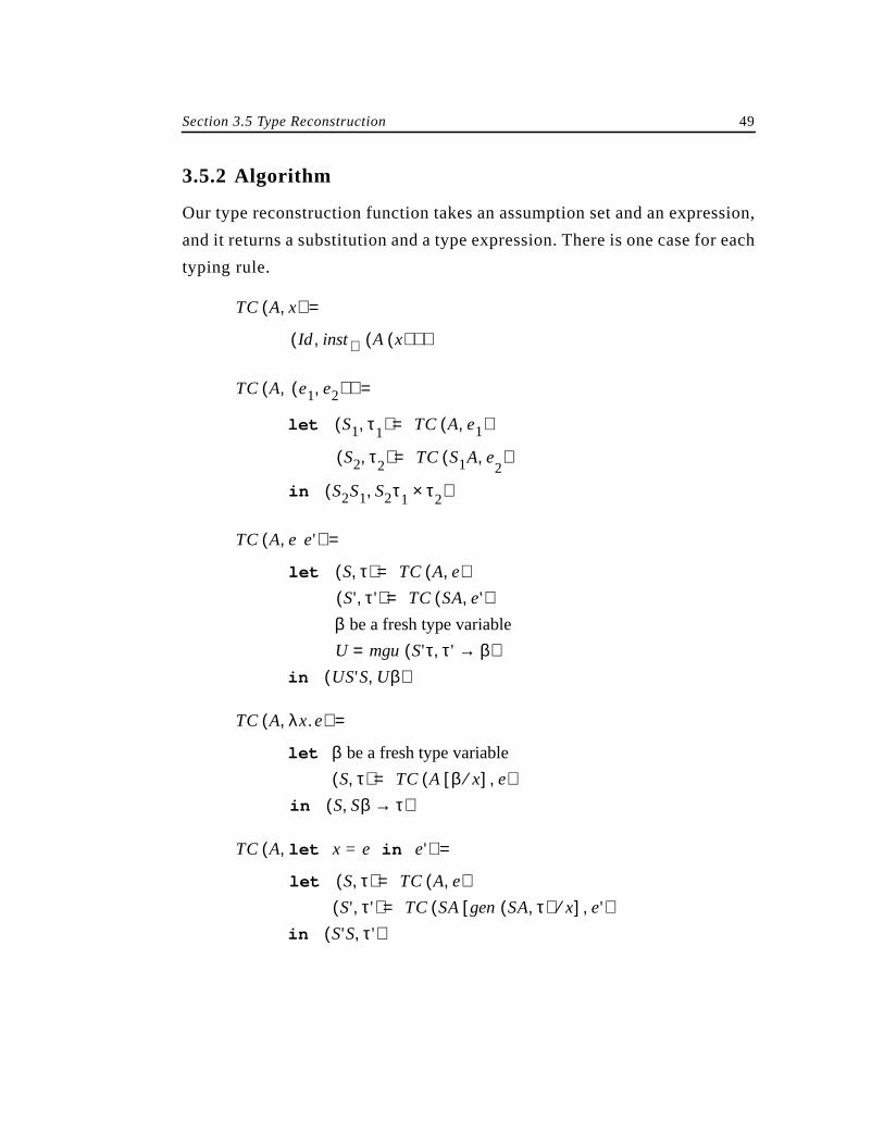
Section 3.5 Type Reconstruction 49
3.5.2 Algorithm
Our type reconstruction function takes an assumption set and an expression,
and it returns a substitution and a type expression. There is one case for each
typing rule.
TC A x,( ) =
Id inst∀ A x( )( ),( )
TC A e1 e2,( ),( ) =
let S1 τ1,( ) = TC A e, 1( )
S2 τ2,( ) = TC S1A e,2
( )
in S2S1 S2τ1 τ2×,( )
TC A e e',( ) =
let S τ,( ) = TC A e,( )S' τ',( ) = TC SA e',( )
β be a fresh type variable
U = mgu S'τ τ' β→,( )in US'S Uβ,( )
TC A λx.e,( ) =
let β be a fresh type variable
S τ,( ) = TC A β x⁄[ ] e,( )in S Sβ τ→,( )
TC A let x = e in e',( ) =
let S τ,( ) = TC A e,( )S' τ',( ) = TC SA gen SAτ,( ) x⁄[ ] e',( )
in S'S τ',( )
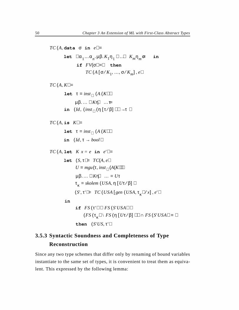
50 Chapter 3 An Extension of ML with First-Class Abstract Types
3.5.3 Syntactic Soundness and Completeness of Type
Reconstruction
Since any two type schemes that differ only by renaming of bound variables
instantiate to the same set of types, it is convenient to treat them as equiva-
lent. This expressed by the following lemma:
TC A data σ in e,( ) =
let α1…αn.∀ µβ.K1η1 … Kmηm+ + σ= in
if FV σ( ) ∅= then
TC A σ K1⁄ … σ Km⁄, ,[ ] e,( )
TC A K,( ) =
let τ inst∀ A K( )( )=
µβ.… Kη …+ + τ=in Id inst∃ η τ β⁄[ ]( )( ) τ→,( )
TC A is K,( ) =
let τ inst∀ A K( )( )=
in Id τ bool→,( )
TC A let K x = e in e',( ) =
let S τ,( ) = TC A e,( )U mgu τ inst∀ A K( )( ),( )=
µβ.… Kη …+ + Uτ=τκ skolem USAη Uτ β⁄[ ],( )=
S' τ',( ) = TC USA gen USAτκ,( ) x⁄[ ] e',( )
in
if FS τ'( ) FS S'USA( )⊆ ∧FS τκ( ) \ FS η Uτ β⁄[ ]( )( ) FS S'USA( )∩ ∅=
then S'US τ',( )
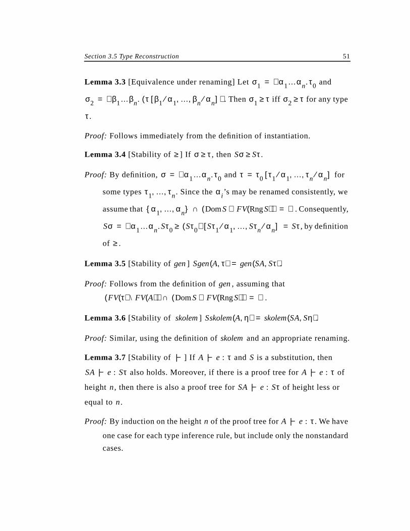
Section 3.5 Type Reconstruction 51
Lemma 3.3 [Equivalence under renaming] Let and
. Then iff for any type
.
Proof: Follows immediately from the definition of instantiation.
Lemma 3.4 [Stability of ] If , then .
Proof: By definition, and for
some types . Since the ’s may be renamed consistently, we
assume that . Consequently,
, by definition
of .
Lemma 3.5 [Stability of ] .
Proof: Follows from the definition of , assuming that
.
Lemma 3.6 [Stability of ] .
Proof: Similar, using the definition of and an appropriate renaming.
Lemma 3.7 [Stability of ] If and is a substitution, then
also holds. Moreover, if there is a proof tree for of
height , then there is also a proof tree for of height less or
equal to .
Proof: By induction on the height of the proof tree for . We have
one case for each type inference rule, but include only the nonstandard
cases.
σ1 α1…αn.∀ τ0=
σ2 β1…βn.∀ τ β1 α1⁄ … βn αn⁄, ,[ ]( )= σ1 τ≥ σ2 τ≥
τ
≥ σ τ≥ Sσ Sτ≥
σ α1…αn.∀ τ0= τ τ0 τ1 α1⁄ … τn αn⁄, ,[ ]=
τ1 … τn, , αi
α1 … αn, , DomS FVRngS( )∪( )∩ ∅=
Sσ α1…αn.∀ Sτ0 Sτ0( ) Sτ1 α1⁄ … Sτn αn⁄, ,[ ]≥ Sτ= =
≥
gen Sgen Aτ,( ) gen SA Sτ,( )=
gen
FV τ( ) \ FV A( )( ) DomS FVRngS( )∪( )∩ ∅=
skolem Sskolem Aη,( ) skolem SA Sη,( )=
skolem
|− A |− e : τ S
SA |− e : Sτ A |− e : τ
n SA |− e : Sτ
n
n A |− e : τ
52 Chapter 3 An Extension of ML with First-Class Abstract Types
The premise is , where
. Since , we have
. By the inductive assumption,
, where
. Finally, we apply
the DATA rule and obtain .
and
The claim follows from stability of under substitution.
Assuming that , we have
and
.
We apply the inductive assumption to the first premise, obtaining
, and to the last premise, obtaining
. Further,
, using
Lemma 3.5 and Lemma 3.6.
Finally, we observe that implies , and
the claim follows by applying the PAT rule.
A |− data α1…αn.∀ µβ.K1η1 … Kmηm+ + in e : τ
A σ K1⁄ … σ Kn⁄, ,[ ] |− e : τ
σ α1…αn.∀ µβ.K1η1 … Kmηm+ += FV σ( ) ∅=
Sσ σ=
S A σ K1⁄ … σ Kn⁄, ,[ ]( ) |− e : Sτ
S A σ K1⁄ … σ Kn⁄, ,[ ]( ) SA( ) σ K1⁄ … σ Kn⁄, ,[ ]=
SA |− data σ in e : Sτ
A |− K : τ µβ.Σ Kη[ ]→
A |− is K : µβ.Σ Kη[ ]( ) bool→
≥
A |− let K x = e in e' : τ'
β DomS FVRngS( )∪∉
S µβ.Σ Kη[ ]( ) µβ.Σ K Sη( )[ ]=
S η µβ.Σ Kη[ ] β⁄[ ]( ) Sη( ) µβ.Σ K Sη( )[ ] β⁄[ ]=
SA |− e : µβ.Σ K Sη( )[ ]
S A gen A skolem Aη µβ.Σ Kη[ ] β⁄[ ],( ),( ) x⁄[ ]( ) |− e' : Sτ'
S A gen A skolem Aη µβ.Σ Kη[ ] β⁄[ ],( ),( ) x⁄[ ]( ) =
SA( ) Sgen A skolem Aη µβ.Σ Kη[ ] β⁄[ ],( ),( ) x⁄[ ] =
SA( ) gen SA skolem SA Sη( ) µβ.Σ K Sη( )[ ] β⁄[ ],( ),( ) x⁄[ ]
FS τ'( ) FS A( )⊆ FS Sτ'( ) FS SA( )⊆
Section 3.5 Type Reconstruction 53
Theorem 3.8[Syntactic soundness] If , then .
Proof: A straightforward application of Lemma 3.7. We show the only
tricky case:
By applying the inductive assumption to the first recursive call to ,
we have . Since succeeds with , we
know that , whence is of the form . By
Lemma 3.7, . We now apply the inductive assump-
tion to the second recursive call and get
.
We use Lemma 3.5 and Lemma 3.6 to obtain
,
where . The subsequent state-
ment ensures that none of the fresh Skolem constructors escape the
scope of the expression. Hence, the PAT rule applies and our
claim is proved.
Definition 3.1 [Principal type] is a principal type of expression under
assumption set if and whenever then there is a sub-
stitution such that .
Theorem 3.9[Syntactic completeness] If , then suc-
ceeds with and there is a substitution such that
and .
Proof: Analogous to the completeness proof given in [Dam85]. We show
only the new cases:
TC A e,( ) S τ,( )= SA |− e : τ
TC A let K x = e in e',( ) S'U τ',( )=
TC
SA |− e : τ mgu τ inst∀ A K( )( ),( ) U
A K( ) Uτ≥ Uτ µβ.Σ Kη[ ]
S'USA |− e : S'Uτ
S' USA gen USA skolem USAη Uτ β⁄[ ],( ),( ) x⁄[ ]( ) |− e' : τ'
S'USA( ) gen S'USA skolem S'USA S' η Uτ β⁄[ ]( ),( ),( ) x⁄[ ] |− e' : τ'
S' η Uτ( ) β⁄[ ]( ) S'η( ) S'Uτ β⁄[ ]= if
let
τ e
A A |− e : τ A |− e : τ'
S Sτ τ'=
SA |− e : τ TC A e,( )
TC A e,( ) S τ,( )= R
SA RSA= τ Rτ=
54 Chapter 3 An Extension of ML with First-Class Abstract Types
Let . Since , we have .
The other premise is , where .
By the inductive assumption, , where there is a sub-
stitution such that and . Hence
succeeds with . Since , also holds,
whence is our desired substitution.
It is clear from the premises that is of the form ,
where ; further, , since must
have been declared in a surrounding expression. Therefore,
, and the instantiations and succeed, such
that , where the and are fresh type
variables. By definition of and , there are types and
such that .
Finally, by choosing , we have
and , since
and
.
This case is analogous to the preceding one.
SA |− data α1…αn.∀ µβ.K1η1 … Kmηm+ + in e : τ
σ α1…αn.∀ µβ.K1η1 …+= FV σ( ) ∅= Sσ σ=
SA' |− e : τ A' A σ K1⁄ … σ Kn⁄, ,[ ]=
TC A' e,( ) S τ,( )=
R SA' RSA'= τ Rτ= TC A data …,( )
S τ,( ) SA' RSA'= SA RSA=
R
SA |− K : τ µβ.Σ Kη[ ]→
SA K( ) σ α1…αn.∀ ρ=
ρ µβ.Σ K β1…βk.∃ τ0[ ]= FV σ( ) ∅= σ
data
SA K( ) A K( )= inst∀ inst∃
τ τ0 ρ→( ) α' i αi⁄ β' j βj⁄,[ ]= α' i β' i
≥ ≤ τ1 … τn, ,
τ'1 … τ'k, , τ µβ.Σ Kη[ ]→ τ0 ρ→( ) τi αi⁄ τ' j βj⁄,[ ]=
R S τi α' i⁄ τ' j β' j⁄,[ ]+=
Rτ τ µβ.Σ Kη[ ]→= RId A SA=
FV τ( ) α'1 … α'n β'1 … β'k, , , , , ⊆
FV A( ) α'1 … α'n β'1 … β'k, , , , , ∩ ∅=
SA |− is K : µβ.Σ Kη[ ]( ) bool→
SA |− let K x = e in e' : τ'ˆ
Section 3.5 Type Reconstruction 55
Again, must be of the form , where
. Therefore, , where the are
new variables. We apply the inductive assumption to the first premise,
, whence and there is an such
that and .
In the first case, , thus . Further,
succeeds with and , there-
fore and . Consequently,
and .
In the second case, , where . Therefore,
succeeds with . Since the occur only in ,
we have and . Further,
and .
In either case, we can apply Lemma 3.7 to the last premise, obtaining
.
By applying Lemma 3.5 and Lemma 3.6, we get
.
Next, the inductive hypothesis gives us , where
, and an such that
and . Then
also holds.
Finally, implies
. This, together with the definition of guar-
SA K( ) A K( )= σ α1…αn.∀ ρ=
ρ µβ.Σ Kη0[ ]= inst∀ σ( ) ρ α' i αi⁄[ ]= α' i
SA |− e : µβ.Σ Kη[ ] TC A e,( ) S τ,( )= R
SA RSA= Rτ µβ.Σ Kη[ ] µβ.Σ K η0 τi αi⁄[ ]( )[ ]= =
τ α= R µβ.Σ K η0 τi αi⁄[ ]( )[ ] α⁄[ ]=
mgu U ρ α' i αi⁄[ ] α⁄[ ]= R τi α' i⁄[ ] U=
RU R= η η0 α' i αi⁄[ ]=
SA RSA RUSA= = η µβ.Σ Kη[ ] β⁄[ ] R η Uτ β⁄[ ]( )=
τ µβ.Σ K η0 τi αi⁄[ ]( )[ ]= Rτi τi=
mgu U τi α' i⁄[ ]= α' i inst∀ σ( )
Uτ τ= η η0 τi αi⁄[ ]= SA RSA RUSA= =
η µβ.Σ Kη[ ] β⁄[ ] R η Uτ β⁄[ ]( )=
RUSA( ) gen RUSA skolem, RUSA R η Uτ β⁄[ ]( ),( )( ) x⁄[ ]( ) |− e' : τ'ˆ
R USA( ) gen USA skolem, USA η Uτ β⁄[ ],( )( ) x⁄[ ]( ) |− e' : τ'ˆ
TC A' e',( ) S' τ',( )=
A' USA gen USA skolem, USA η Uτ β⁄[ ],( )( ) x⁄[ ]= R'
RA' R'S'A'= τ'ˆ R'τ'= R'S'USA RUSA RSA SˆA= = =
FS τ'ˆ( ) FS R'τ'( )= FS SA( ) FS R'S'USA( )=⊆
FS τ'( ) FS S'USA( )⊆ skolem
56 Chapter 3 An Extension of ML with First-Class Abstract Types
antees that the statement succeeds. Consequently,
succeeds with , and is the desired substitution.
Corollary 3.10 [Principal type] If , then is a principal
type for under .
3.6 Semantics
We give a standard denotational semantics. The evaluation function maps
an expression to some semantic value , in the context of an eval-
uation environment . An evaluation environment is a partial map-
ping from identifiers to semantic values. Runtime type errors are represent-
ed by the special value . Tagged values are used to capture the seman-
tics of algebraic data types.
We distinguish between the three error situations, runtime type errors
( ), nontermination, and a mismatch when an attempt is made to de-
compose a tagged value whose tag does not match the tag of the destructor.
Both nontermination and mismatch are expressed by .
Our type inference system is sound with respect to the evaluation func-
tion; a well-typed program never evaluates to . The formal proof for
semantic soundness is given below.
It should be noted that we do not commit ourselves to a strict or non-
strict evaluation function. Therefore, our treatment of existential types ap-
plies to languages with both strict and non-strict semantics. In either case,
appropriate conditions would have to be added to the definition of the eval-
uation function for pair expressions, function applications,let expressions,
and pattern-matchinglet expressions: the strict evaluation function returns
whenever a subexpression evaluates to , while the non-strict evaluation
function retains as the value of that subexpression.
if TC A let …,( )
S'US τ',( ) R'
TC A e,( ) S τ,( )= τ
e A
E
e Exp∈ v
ρ Env∈
wrong
wrong
⊥
wrong
⊥ ⊥
⊥
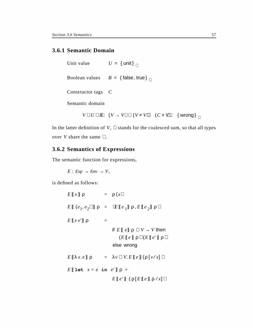
Section 3.6 Semantics 57
3.6.1 Semantic Domain
Unit value
Boolean values
Constructor tags
Semantic domain
In the latter definition of , stands for the coalesced sum, so that all types
over share the same .
3.6.2 Semantics of Expressions
The semantic function for expressions,
,
is defined as follows:
=
=
=
=
=
U unit ⊥=
B false true, ⊥=
C
V U B V V→( ) V V×( ) C V×( ) wrong ⊥+ + ++ +≅
V +
V ⊥
E : Exp Env V→ →
E [[ x ]] ρ ρ x( )
E [[ e1 e2,( ) ]] ρ E [[ e1]] ρ E [[ e2]] ρ,⟨ ⟩
E [[ e e']] ρ
if E [[ e]] ρ V V→∈ then
E [[ e]] ρ( ) E [[ e' ]] ρ( )else wrong
E [[ λ x.e]] ρ λv V∈ .E [[ e]] ρ v x⁄[ ]( )
E [[ let x = e in e' ]] ρ
E [[ e' ]] ρ E [[ e]] ρ x⁄[ ]( )
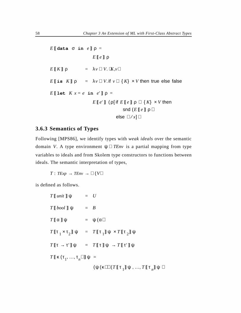
58 Chapter 3 An Extension of ML with First-Class Abstract Types
=
=
=
=
3.6.3 Semantics of Types
Following [MPS86], we identify types withweak ideals over the semantic
domain . A type environment is a partial mapping from type
variables to ideals and from Skolem type constructors to functions between
ideals. The semantic interpretation of types,
is defined as follows.
=
=
=
=
=
=
E [[ data σ in e]] ρ
E [[ e]] ρ
E [[ K ]] ρ λv V∈ . K v,⟨ ⟩
E [[ is K ]] ρ λv V∈ . if v K V×∈ then true else false
E [[ let K x = e in e' ]] ρ
E [[ e' ]] ( ρ[ if E [[ e]] ρ K V×∈ then
snd E [[ e]] ρ( )else ⊥ x⁄ ] )
V ψ TEnv∈
T : TExp TEnv ℑ V( )→ →
T [[ unit ]] ψ U
T [[ bool ]] ψ B
T [[ α ]] ψ ψ α( )
T [[ τ 1 τ2× ]] ψ T [[ τ 1]] ψ T [[ τ 2]] ψ×
T [[ τ τ'→ ]] ψ T [[ τ ]] ψ T [[ τ' ]] ψ→
T [[ κ τ1 … τn, ,( ) ]] ψ
ψ κ( )( ) T [[ τ 1]] ψ … T [[ τ n]] ψ, ,( )
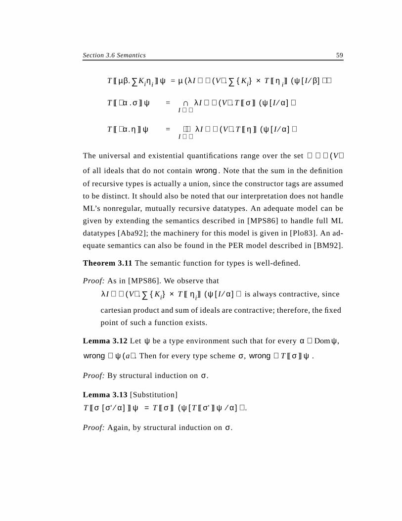
Section 3.6 Semantics 59
=
=
=
The universal and existential quantifications range over the set
of all ideals that do not contain . Note that the sum in the definition
of recursive types is actually a union, since the constructor tags are assumed
to be distinct. It should also be noted that our interpretation does not handle
ML’s nonregular, mutually recursive datatypes. An adequate model can be
given by extending the semantics described in [MPS86] to handle full ML
datatypes [Aba92]; the machinery for this model is given in [Plo83]. An ad-
equate semantics can also be found in the PER model described in [BM92].
Theorem 3.11The semantic function for types is well-defined.
Proof: As in [MPS86]. We observe that
is always contractive, since
cartesian product and sum of ideals are contractive; therefore, the fixed
point of such a function exists.
Lemma 3.12Let be a type environment such that for every ,
. Then for every type scheme , .
Proof: By structural induction on .
Lemma 3.13[Substitution]
.
Proof: Again, by structural induction on .
T [[ µβ. Kiηi∑ ]] ψ µ λI ℑ V( )∈ . Ki T [[ η i]] ψ I β⁄[ ]( )×∑( )
T [[ α .σ∀ ]] ψ λI ℑ V( )∈ .T [[ σ ]] ψ I α⁄[ ]( )I ℜ∈∩
T [[ α.η∃ ]] ψ I ℜ∈
λI ℑ V( )∈ .T [[ η ]] ψ I α⁄[ ]( )
ℜ ℑ V( )⊆
wrong
λI ℑ V( )∈ . Ki T [[ ηi]] ψ I α⁄[ ]( )×∑
ψ α Domψ∈
wrong ψ a( )∉ σ wrong T [[ σ ]] ψ∉
σ
T [[ σ σ' α⁄[ ] ]] ψ T [[ σ ]] ψ T [[ σ' ]] ψ α⁄[ ]( )=
σ
60 Chapter 3 An Extension of ML with First-Class Abstract Types
Definition 3.2 [Semantic type judgment] Let be an assumption set, an
expression, and a type scheme. We define as meaning that
and for every , ; further, we
say iff implies ; and finally,
means that for all and we have .
Theorem 3.14[Semantic soundness] If then .
Proof: By induction on the size of the proof tree for . We need to
consider each of the cases given by the type inference rules. Applying
the inductive assumption and the typing judgments from the preceding
steps in the type derivation, we use the semantics of the types of the
partial results of the evaluation. In each of the cases below, choose
and arbitrarily, such that . We include only the nonstandard
cases. Lemma 3.13 will be used with frequency.
The premise in the type derivation is ,
where . Since by definition,
, we can use the inductive assumption to ob-
tain .
The last premise in the type derivation is , where
. By definition of instantiation of existential types,
A e
σ |= ρ ψ, A
DomA Domρ⊆ x DomA∈ ρ x( ) T [[ A x( ) ]] ψ∈
A |= ρ ψ, e : σ |= ρ ψ, A E [[ e]] ρ T [[ σ ]] ψ∈
A |= e : σ ρ Env∈ ψ TEnv∈ A |= ρ ψ, e : σ
A |− e : τ A |= e : τ
A |− e : τ
ψ
ρ |= ρ ψ, A
A |− data α1…αn.∀ µβ.K1η1 … Kmηm+ + in e : τ
A σ K1⁄ … σ Km⁄, ,[ ] |− e : τ
σ α1…αn.∀ µβ.K1η1 … Kmηm+ +=
|= ρ ψ, A σ K1⁄ … σ Km⁄, ,[ ]
E [[ data α1…αn.∀ χ in e]] ρ E [[ e]] ρ= T [[ τ ]] ψ∈
A |− K : τ µβ.Σ Kη[ ]→
η µβ.Σ Kη[ ] β⁄[ ] τ≤
η γ1…γn.∃ τ=
Section 3.6 Semantics 61
for some types .
First, choose an arbitrary and a finite . Now,
=
⊆
=
= .
Hence, , by
closure of ideals under limits. Consequently,
⊆
=
= .
Hence .
Choose an arbitrary . Clearly,
, whence
.
We follow the proofs in [Dam85] and [MPS86]. The first premise in the
type derivation is , where and
. Let . Then, for arbi-
τ τ τj γj⁄ µβ.Σ Kη[ ] β⁄,[ ]= τ1 … τn, ,
v T [[ τ ]] ψ∈ a v≤
a ∈ T [[ τ τj γj⁄ µβ.Σ Kη[ ] β⁄,[ ] ]] ψ( ) °
T [[ τ µβ.Σ Kη[ ] β⁄[ ] ]] ψ T [[ τ j]] ψ γj⁄[ ]( )( ) °
T [[ τ µβ.Σ Kη[ ] β⁄[ ] ]] ψ Jj γj⁄[ ]( )( ) °J1 … Jn, , ℜ∈
∪
J1 … Jn, , ℜ∈
T [[ τ µβ.Σ Kη[ ] β⁄[ ] ]] ψ Jj γj⁄[ ]( )( ) °
T [[ η µβ.Σ Kη[ ] β⁄[ ] ]] ψ( ) °
v a a finite and a v≤ T [[ η µβ.Σ Kη[ ] β⁄[ ] ]] ψ∈=
K v,⟨ ⟩ ∈ K T [[ η µβ.Σ Kη[ ] β⁄[ ] ]] ψ×
… K T [[ η µβ.Σ Kη[ ] β⁄[ ] ]] ψ× …+ +
… K T [[ η ]] ψ T [[ µβ.Σ Kη[ ] ]] ψ β⁄[ ]( )× …+ +
T [[ µβ.Σ Kη[ ] ]] ψ
E [[ K ]] ρ T [[ τ µβ.Σ Kη[ ]→ ]] ψ∈
A |− is K : µβ.Σ Kη[ ]( ) bool→
v T [[ µβ.Σ Kη[ ] ]] ψ∈
E [[ is K ]] ρ( ) v B∈
E [[ is K ]] ρ T [[ µβ.Σ Kη[ ]( ) bool→ ]] ψ∈
A |− let K x = e in e' : τ'
A |− e : τ τ µβ.Σ Kη[ ]=
η γ1…γn.∃ τ= α1 … αk, , FV τ( ) \ FV A( )=
62 Chapter 3 An Extension of ML with First-Class Abstract Types
trary , holds, since none of the ’s
are free in .
Let ; by the inductive assumption,
. Consequently,
=
=
.
First, consider the more interesting case, . Then
Let , , be those variables among that are free
in .
We now choose a finite such that , thus
.
I1 … Ik ℜ∈, , |= ρ ψ I i αi⁄ i = 1…k[ ], A αi
A
v E [[ e]] ρ=
v T [[ τ ]] ψ I i αi⁄[ ]( )∈
v ∈ T [[ τ ]] ψ I i αi⁄[ ]( )I1 … Ik, , ℜ∈
∩
T [[ µβ.Σ Kη[ ] ]] ψ I i αi⁄[ ]( )I1 … Ik, , ℜ∈
∩
… +
K T [[ η ]] ψ I i αi⁄ T [[ τ ]] ψ I i αi⁄[ ]( ) β⁄,[ ]( )I1 … Ik, , ℜ∈
∩×
…+
fst v( ) = K
snd v( ) J1 … Jn, , ℜ∈I1 … Ik, , ℜ∈
∩∈
T [[ τ ]] ψ I i αi⁄ Jj γj⁄ T [[ τ ]] ψ I i αi⁄[ ]( ) β⁄, ,[ ]( )
α1 … αh, , h k≤ α1 … αk, ,
τ τ β⁄[ ]
a a snd v( )≤
a T [[ τ τ β⁄[ ] ]] ψ I i αi⁄ Jj γj⁄,[ ]( )( ) °J1 … Jn, , ℜ∈
∪I1 … Ih, , ℜ∈
∩∈
Section 3.6 Semantics 63
By definition of set union and intersection, there exist functions
,
such that
⊆
=
=
= ,
assuming that the ’s are the ones generated by .
Since by definition of , none of the ’s are free in ,
holds and we can extend and , obtaining
.
We now apply the inductive assumption to the last premise,
,
and obtain
,
since . Finally,
=
= ,
by the continuity of . The latter expression is in by the clo-
sure of ideals under limits.
f1 … fn ℑ V( ) h ℑ V( )→∈, ,
a ∈ T [[ τ τ β⁄[ ] ]] ψ I i αi⁄ fj I1 … Ih, ,( ) γj⁄,[ ]( )( ) °I1 … Ih, , ℜ∈
∩
T [[ τ τ β⁄[ ] ]] ψ I i αi⁄ fj I1 … Ih, ,( ) γj⁄,[ ]( )I1 … Ih, , ℜ∈
∩
T [[ τ κj α1 … αh, ,( ) γj⁄ τ β⁄,[ ] ]] ψ I i αi⁄ fj κj⁄,[ ]( )I1 … Ih, , ℜ∈
∩
T [[ α 1…αh∀ . τ κj α1 … αh, ,( ) γj⁄ τ β⁄,[ ] ]] ψ fj κj⁄[ ]( )
T [[ gen A skolem Aη τ β⁄[ ],( ),( ) ]] ψ fj κj⁄[ ]( )
κj skolem Aη τ β⁄[ ],( )
skolem κj A
|= ρ ψ fj κj⁄[ ], A A ρ
|= ρ a x⁄[ ] ψ fj κj⁄[ ], A gen A skolem Aη τ β⁄[ ],( ),( ) x⁄[ ]
A gen A skolem Aη τ β⁄[ ],( ),( ) x⁄[ ] |− e' : τ'
E [[ e' ]] ρ a x⁄[ ]( ) T [[ τ' ]] ψ fj κj⁄[ ]( )∈ T [[ τ' ]] ψ=
FS τ'( ) FS A( )⊆
E [[ let K x = e in e' ]] ρ
E [[ e' ]] ρ snd E [[ e]] ρ( ) x⁄[ ]( )
E [[ e' ]] ρ a x⁄[ ]( ) a finite and a snd E [[ e]] ρ( )≤
E T [[ τ' ]] ψ
64 Chapter 3 An Extension of ML with First-Class Abstract Types
In the second case, . For any functions
we have . Again,
since none of the ’s are free in , holds and we can
extend and , obtaining
.
By applying the inductive assumption to the last premise,
,
we obtain
.
This concludes our proof of semantic soundness.
Corollary 3.15 [Semantic soundness] Let be a type environment such
that for every , . If and , then
.
Proof: We apply Lemma 3.12 to Theorem 3.14.
fst v( ) K≠ f1 … fn, , ℑ V( )h ℑ V( )→∈
⊥ T [[ gen A skolem Aη τ β⁄[ ],( ),( ) ]] ψ fj κj⁄[ ]( )∈
κj A |= ρ ψ fj κj⁄[ ], A
A ρ
|= ρ ⊥ x⁄[ ] ψ fj κj⁄[ ], A gen A skolem Aη τ β⁄[ ],( ),( ) x⁄[ ]
A gen A skolem Aη τ β⁄[ ],( ),( ) x⁄[ ] |− e' : τ'
E [[ e' ]] ρ ⊥ x⁄[ ]( ) T [[ τ' ]] ψ fj κj⁄[ ]( )∈ T [[ τ' ]] ψ=
ψ
α Domψ∈ wrong ψ a( )∉ A |− e : τ |= ρ ψ, A
E [[ e]] ρ wrong≠
65
4 An Extension of ML with aDotless Dot Notation
In this chapter, we describe a extension of our language that allows more
flexible use of existential types. Following notations used in actual pro-
gramming languages, this extension assumes the same representation type
each time a value of existential type is accessed, provided that each access
is through the same identifier. We give a type reconstruction algorithm and
show semantic soundness by translating into the language from Chapter 3.
4.1 Introduction
MacQueen [Mac86] observes that the use of existential types in connection
with an elimination construct (open , abstype , or our let ) is impractical
in certain programming situations; often, the scope of the elimination con-
struct has to be made so large that some of the benefits of abstraction are
lost. In particular, the lowest-level entities have to be opened at the outer-
most level; these are the traditional disadvantages of block-structured lan-
guages.
We present an extension of ML that provides the same flexibility as the
dot notation described in [CL90]. In this extension, abstract types are again
modeled by ML datatypes with existentially quantified component types.
Values of abstract type are created by applying a datatype constructor to a
66 Chapter 4 An Extension of ML with a Dotless Dot Notation
value, and they are decomposed in a pattern-matchinglet expression.
However, we allow existentially quantified type variables to escape the
scope of the identifier in whose type they appear, as long as the expression
decomposed is an identifier and the existentially quantified type variables do
not escape the scope of that identifier. Each decomposition of an identifier,
using the same constructor, produces identical existentially quantified type
variables. We call our notation a “dotless” dot notation, since it uses decom-
position by pattern-matching instead of record component selection.
4.2 Some Motivating Examples
We assume the type declaration
datatype Key = key of ’a * (’a -> int)
in the following examples. In the first example,
let val x = key(3,fn x => x + 2) in
(let val key(_,f) = x in f end)
(let val key(v,_) = x in v end)
end
the existential type variable in the type off is the same as the one in the type
of v, and the function application produces a result of typeint . This follows
from the fact that bothf and v are bound by decomposition of the same1
identifier,x . Consequently, they must hold the same value and the whole ex-
pression is type-correct.
1We assume the ML scoping discipline, which useslet statements as scopeboundaries; alternatively, one could require each bound identifier to be unique.
Section 4.2 Some Motivating Examples 67
In a language with the traditional dot notation, for example Ada, abstract
types can be modeled as packages, and an example corresponding to the pre-
vious one would look as follows:
package KEY_PKG is
type KEY is private;
X : constant KEY;
function F(X : KEY) return INTEGER;
private
type KEY is INTEGER;
X : constant KEY := 3;
end KEY_PKG;
package body KEY_PKG is
function F(X : KEY) return INTEGER is
begin
return X + 2;
end;
end KEY_PKG;
var Z : INTEGER;
...
Z := KEY_PKG.F(KEY_PKG.X);
The components of the abstract typeKEY_PKG are selected using the dot no-
tation.
The following are examples of incorrect programs. For instance,
let val x = key(3,fn x => x + 2) in
let val key(_,f) = x in
f
end
end
68 Chapter 4 An Extension of ML with a Dotless Dot Notation
is not type-correct, since the existential type variable in the type off es-
capes the scope ofx . Neither is the following program,
let val x = key(3,fn x => x + 2)
val y = x
in
(let val key(_,f) = x in f end)
(let val key(v,_) = y in v end)
end
since different identifiers produce different existential type variables, al-
though they hold the same values in this case. As the latter cannot be deter-
mined statically, we must assume that the values have different types. Sim-
ilarly,
val z = (3,fn x => x + 2)
let val key(_,f) = key z in
let val key(v,_) = key z in
f v
end
end
is not type-correct. Since the expressions that are decomposed are not even
identifiers, we cannot assume statically thatf can be applied tov.
4.3 Syntax
4.3.1 Language Syntax
Syntactically, our underlying formal language is almost unchanged, except
that pattern-matchinglet expressions only allow an identifier to be decom-
posed, not a general expression. This is not a significant restriction, since
we can always bind the expression in an enclosinglet before decomposing
it. Again, we assume that each identifier bound by a or expression is
unique.
Identifiers
λ let
x
Section 4.3 Syntax 69
Constructors
Type constructors
Expressions ::= | | |
| | | |
|
| | |
4.3.2 Type Syntax
Type variables
Skolem functions
Types ::= | | | | |
|
Recursive types ::= where for
Existential types ::= |
Type schemes ::= |
Assumptions ::= |
Our type syntax is almost unchanged. However, Skolem type constructors
are now uniquely associated with an identifier by using the symbol , in-
dexed by , the constructor used in the decomposition, and the index of
the existentially quantified variable to be replaced.
K
T
e () true false
x e1 e2,( ) e e' λx.e
let x = e in e'
data α1…αn.∀ χ in e K is K
let K x x'= in e'
α
κ
τ unit bool α τ1 τ2× τ τ'→
κx K i, , τ1 … τn, ,( ) χ
χ µβ.K1η1 … Kmηm+ + Ki Kj≠
i j≠
η α.η∃ τ
σ α.σ∀ τ
a σ x⁄ α1…αn.∀ χ
x κ
x K i
γi
70 Chapter 4 An Extension of ML with a Dotless Dot Notation
4.4 Type Inference
4.4.1 Instantiation and Generalization of Type Schemes
iff there are types such that
iff there are types such that
=
=
where
Instantiation and generalization are unchanged. The modified function
replaces each existentially quantified variable in a type by a unique
type constructor whose actual arguments are those free variables of the type
that are not free in the assumption set. Since identifiers are unique, we ob-
tain Skolem constructors uniquely associated with an identifier by using
the symbol , indexed by , the constructor used in the decomposition,
and the index of the existentially quantified variable to be replaced. In
addition to , the set of free type variables in a type scheme or assumption
set, we use , the set of those Skolem type constructors that occur in a
type scheme or assumption set and are associated with identifier .
4.4.2 Inference Rules for Expressions
The first three typing rules are the same as in the original system.
α1…αn.τ∀ τ'≥ τ1 …τn,
τ' τ τ1 α1⁄ … τn αn⁄, ,[ ]=
α1…αn.τ∃ τ'≤ τ1 …τn,
τ' τ τ1 α1⁄ … τn αn⁄, ,[ ]=
gen A τ,( ) FV τ( ) \ FV A( )( ) .τ∀
skolem. A x K γ1…γn.τ∃, , ,( )
τ κx K i, , α1 …αk,( ) γi⁄[ ]
α1 … αk, , FV γ1…γn.τ∃( ) \ FV A( )=
skolem.
x
κ x K
i γi
FV
FSx
x
Section 4.4 Type Inference 71
(VAR.)
(PAIR.)
(APPL.)
The ABS. and LET. rules are modified to prevent Skolem constructors asso-
ciated with a bound variable to escape the scope of that variable.
(ABS.)
(LET.)
The rules DATA., CONS., TEST. remain unchanged.
(DATA .)
(CONS.)
A x( ) τ≥A |−. x : τ
A |−. e1 : τ1 A |−. e2 : τ2
A |−. e1 e2,( ) : τ1 τ2×
A |−. e : τ' → τ A |−. e' : τ'
A |−. e e' : τ
A τ' x⁄[ ] |−. e : τ FSx A( ) FSx τ( )∪ ∅=
A |−. λx.e : τ' τ→
A |−. e : τ
A gen A τ,( ) x⁄[ ] |−. e' : τ' FSx A( ) FSx τ'( )∪ ∅=
A |−.let x = e in e' : τ'
σ α1…αn.∀ µβ.K1η1 … Kmηm+ +=
FV σ( ) ∅= A σ K1⁄ … σ Km⁄, ,[ ] |−. e : τ
A |−.data σ in e : τ
A K( ) µβ.Σ Kη[ ]≥ η µβ.Σ Kη[ ] β⁄[ ] τ≤A |−. K : τ µβ.Σ Kη[ ]→
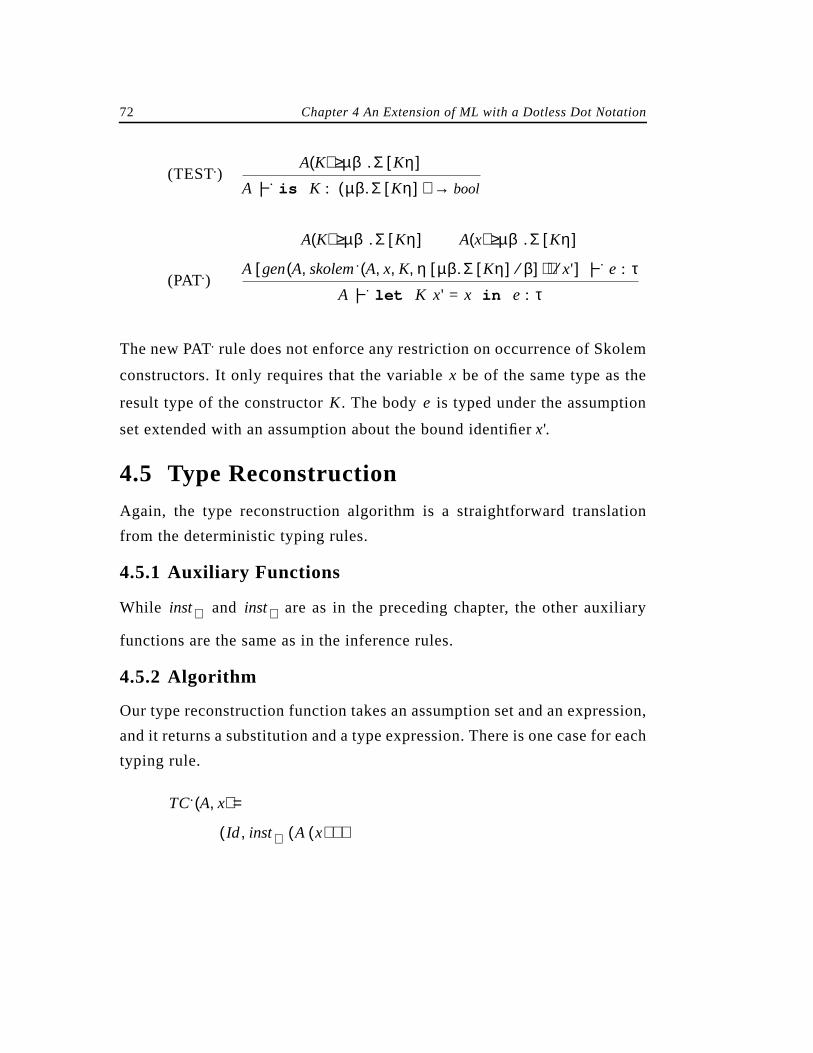
72 Chapter 4 An Extension of ML with a Dotless Dot Notation
(TEST.)
(PAT.)
The new PAT. rule does not enforce any restriction on occurrence of Skolem
constructors. It only requires that the variable be of the same type as the
result type of the constructor . The body is typed under the assumption
set extended with an assumption about the bound identifier .
4.5 Type Reconstruction
Again, the type reconstruction algorithm is a straightforward translation
from the deterministic typing rules.
4.5.1 Auxiliary Functions
While and are as in the preceding chapter, the other auxiliary
functions are the same as in the inference rules.
4.5.2 Algorithm
Our type reconstruction function takes an assumption set and an expression,
and it returns a substitution and a type expression. There is one case for each
typing rule.
A K( ) µβ.Σ Kη[ ]≥A |−.
is K : µβ.Σ Kη[ ]( ) bool→
A K( ) µβ.Σ Kη[ ]≥ A x( ) µβ.Σ Kη[ ]≥
A gen A skolem. A x K η µβ.Σ Kη[ ] β⁄[ ], , ,( ),( ) x'⁄[ ] |−. e : τA |−.
let K x' = x in e : τ
x
K e
x'
inst∀ inst∃
TC. A x,( ) =
Id inst∀ A x( )( ),( )
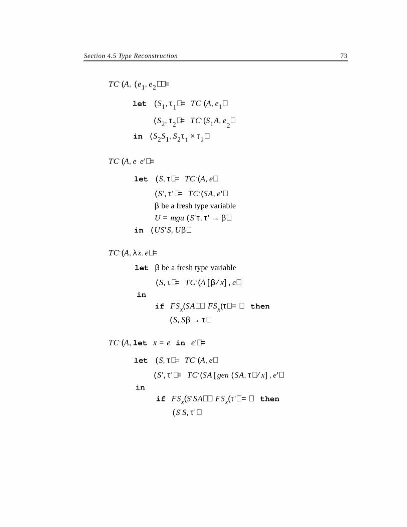
Section 4.5 Type Reconstruction 73
TC. A e1 e2,( ),( ) =
let S1 τ1,( ) = TC. A e, 1( )
S2 τ2,( ) = TC. S1A e,2
( )
in S2S1 S2τ1 τ2×,( )
TC. A e e',( ) =
let S τ,( ) = TC. A e,( )
S' τ',( ) = TC. SA e',( )β be a fresh type variable
U = mgu S'τ τ' β→,( )in US'S Uβ,( )
TC. A λx.e,( ) =
let β be a fresh type variable
S τ,( ) = TC. A β x⁄[ ] e,( )in
if FSx SA( ) FSx τ( )∪ ∅= then
S Sβ τ→,( )
TC. A let x = e in e',( ) =
let S τ,( ) = TC. A e,( )
S' τ',( ) = TC. SA gen SAτ,( ) x⁄[ ] e',( )in
if FSx S'SA( ) FSx τ'( )∪ ∅= then
S'S τ',( )
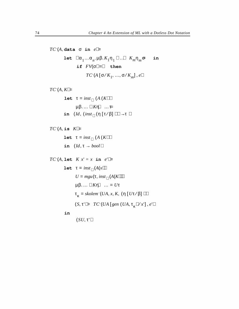
74 Chapter 4 An Extension of ML with a Dotless Dot Notation
TC. A data σ in e,( ) =
let α1…αn.∀ µβ.K1η1 … Kmηm+ + σ= in
if FV σ( ) ∅= then
TC. A σ K1⁄ … σ Km⁄, ,[ ] e,( )
TC. A K,( ) =
let τ inst∀ A K( )( )=
µβ.… Kη …+ + τ=in Id inst∃ η τ β⁄[ ]( )( ) τ→,( )
TC. A is K,( ) =
let τ inst∀ A K( )( )=
in Id τ bool→,( )
TC. A let K x' = x in e',( ) =
let τ = inst∀ A x( )( )
U mgu τ inst∀ A K( )( ),( )=
µβ.… Kη …+ + Uτ=
τκ skolem. UA x K η Uτ β⁄[ ]( ), , ,( )=
S τ',( ) = TC. UA gen UA τκ,( ) x'⁄[ ] e',( )
in
SU τ',( )
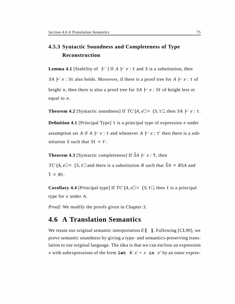
Section 4.6 A Translation Semantics 75
4.5.3 Syntactic Soundness and Completeness of Type
Reconstruction
Lemma 4.1 [Stability of ] If and is a substitution, then
also holds. Moreover, if there is a proof tree for of
height , then there is also a proof tree for of height less or
equal to .
Theorem 4.2[Syntactic soundness] If , then .
Definition 4.1 [Principal Type] is a principal type of expression under
assumption set if and whenever then there is a sub-
stitution such that .
Theorem 4.3[Syntactic completeness] If , then
and there is a substitution such that and
.
Corollary 4.4 [Principal type] If , then is a principal
type for under .
Proof: We modify the proofs given in Chapter 3.
4.6 A Translation Semantics
We retain our original semantic interpretation . Following [CL90], we
prove semantic soundness by giving a type- and semantics-preserving trans-
lation to our original language. The idea is that we can enclose an expression
with subexpressions of the form by an outer expres-
|−. A |−. e : τ S
SA |−. e : Sτ A |−. e : τ
n SA |−. e : Sτ
n
TC. A e,( ) S τ,( )= SA |−. e : τ
τ e
A A |−. e : τ A |−. e : τ'
S Sτ τ'=
SA |−. e : τ
TC. A e,( ) S τ,( )= R SA RSA=
τ Rτ=
TC. A e,( ) S τ,( )= τ
e A
E [[ ]]
e let K x' = x in e'
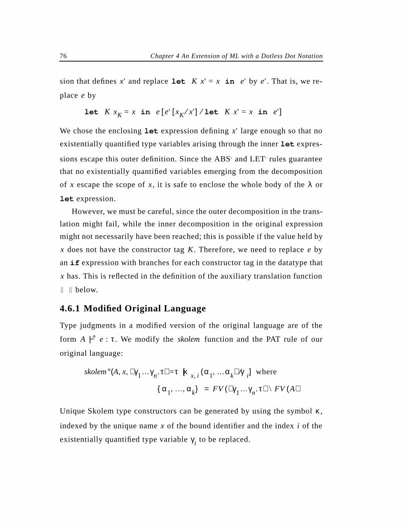
76 Chapter 4 An Extension of ML with a Dotless Dot Notation
sion that defines and replace by . That is, we re-
place by
We chose the enclosinglet expression defining large enough so that no
existentially quantified type variables arising through the innerlet expres-
sions escape this outer definition. Since the ABS. and LET. rules guarantee
that no existentially quantified variables emerging from the decomposition
of escape the scope of , it is safe to enclose the whole body of the or
let expression.
However, we must be careful, since the outer decomposition in the trans-
lation might fail, while the inner decomposition in the original expression
might not necessarily have been reached; this is possible if the value held by
does not have the constructor tag . Therefore, we need to replace by
an if expression with branches for each constructor tag in the datatype that
has. This is reflected in the definition of the auxiliary translation function
below.
4.6.1 Modified Original Language
Type judgments in a modified version of the original language are of the
form . We modify the function and the PAT rule of our
original language:
= where
Unique Skolem type constructors can be generated by using the symbol ,
indexed by the unique name of the bound identifier and the index of the
existentially quantified type variable to be replaced.
x' let K x' = x in e' e'
e
let K xK = x in e e' xK x'⁄[ ] let K x' = x in e'⁄[ ]
x'
x x λ
x K e
x
A |−° e : τ skolem
skolem° A x γ1…γn.τ∃, ,( ) τ κx i, α1 …αk,( ) γi⁄[ ]
α1 … αk, , FV γ1…γn.τ∃( ) \ FV A( )=
κ
x i
γi
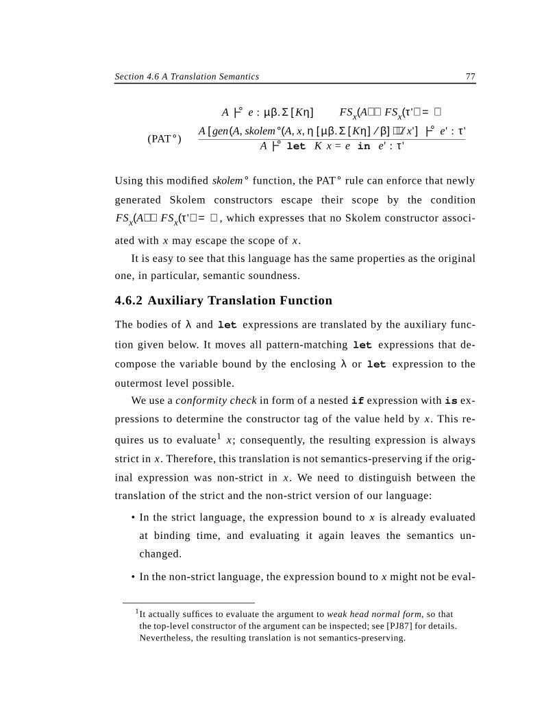
Section 4.6 A Translation Semantics 77
(PAT )
Using this modified function, the PAT rule can enforce that newly
generated Skolem constructors escape their scope by the condition
, which expresses that no Skolem constructor associ-
ated with may escape the scope of .
It is easy to see that this language has the same properties as the original
one, in particular, semantic soundness.
4.6.2 Auxiliary Translation Function
The bodies of and expressions are translated by the auxiliary func-
tion given below. It moves all pattern-matching expressions that de-
compose the variable bound by the enclosing or expression to the
outermost level possible.
We use aconformity check in form of a nestedif expression withis ex-
pressions to determine the constructor tag of the value held by . This re-
quires us to evaluate1 ; consequently, the resulting expression is always
strict in . Therefore, this translation is not semantics-preserving if the orig-
inal expression was non-strict in . We need to distinguish between the
translation of the strict and the non-strict version of our language:
• In the strict language, the expression bound to is already evaluated
at binding time, and evaluating it again leaves the semantics un-
changed.
• In the non-strict language, the expression bound to might not be eval-
1It actually suffices to evaluate the argument toweak head normal form, so thatthe top-level constructor of the argument can be inspected; see [PJ87] for details.Nevertheless, the resulting translation is not semantics-preserving.
°
A |−° e : µβ.Σ Kη[ ] FSx A( ) FSx τ'( )∪ ∅=
A gen A skolem° A x η µβ.Σ Kη[ ] β⁄[ ], ,( ),( ) x'⁄[ ] |−° e' : τ'A |−° let K x = e in e' : τ'
skolem° °
FSx A( ) FSx τ'( )∪ ∅=
x x
λ let
let
λ let
x
x
x
x
x
x
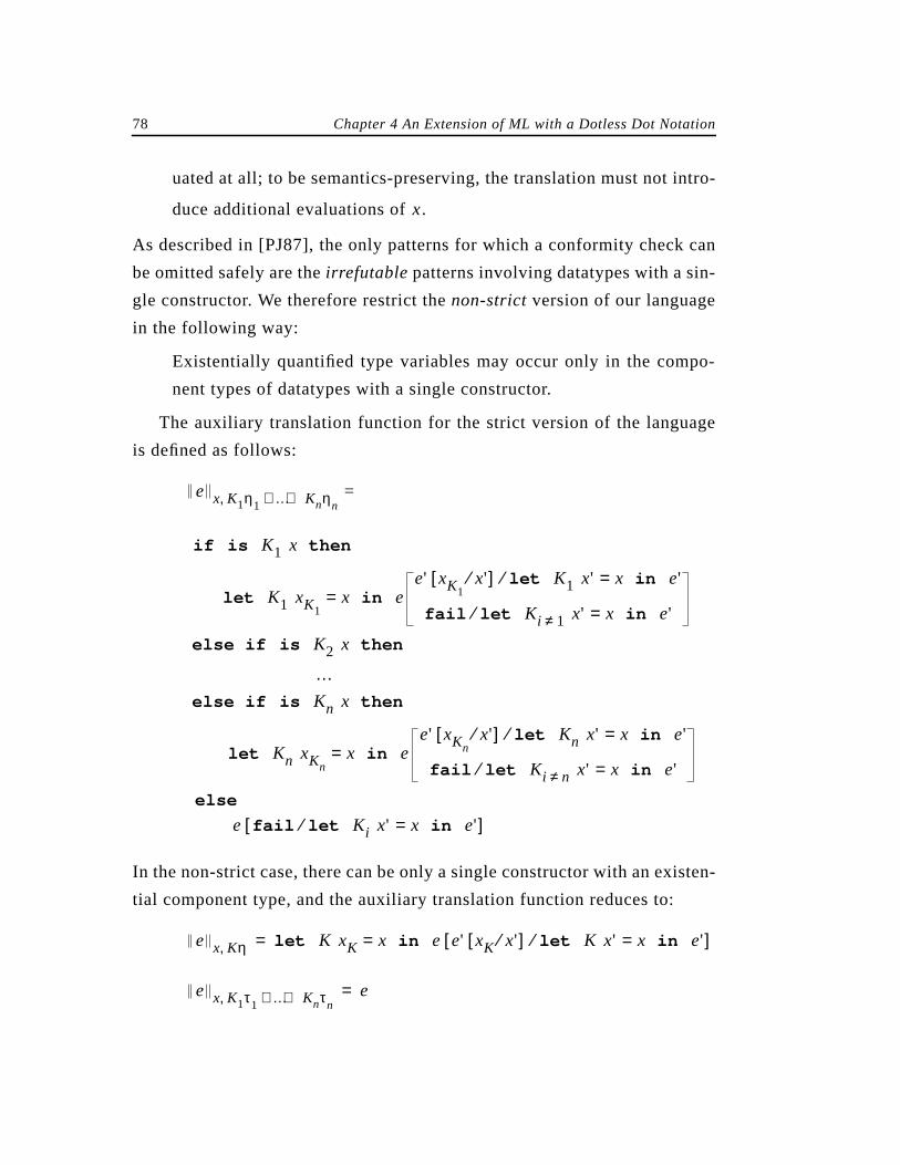
78 Chapter 4 An Extension of ML with a Dotless Dot Notation
uated at all; to be semantics-preserving, the translation must not intro-
duce additional evaluations of .
As described in [PJ87], the only patterns for which a conformity check can
be omitted safely are theirrefutable patterns involving datatypes with a sin-
gle constructor. We therefore restrict thenon-strict version of our language
in the following way:
Existentially quantified type variables may occur only in the compo-
nent types of datatypes with a single constructor.
The auxiliary translation function for the strict version of the language
is defined as follows:
=
In the non-strict case, there can be only a single constructor with an existen-
tial component type, and the auxiliary translation function reduces to:
x
e x K1η1 … Knηn+ +,
if is K1 x then
let K1 xK1x= in e
e' xK1x'⁄[ ] let K1 x' x= in e'⁄
fail let Ki 1≠ x' x= in e'⁄
else if is K2 x then
…else if is Kn x then
let Kn xKnx= in e
e' xKnx'⁄[ ] let Kn x' x= in e'⁄
fail let Ki n≠ x' x= in e'⁄
else
e fail let Ki x' x= in e'⁄[ ]
e x Kη, let K xK x= in e e' xK x'⁄[ ] let K x' x= in e'⁄[ ]=
e x K1τ1 … Knτn+ +, e=
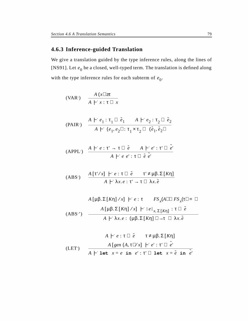
Section 4.6 A Translation Semantics 79
4.6.3 Inference-guided Translation
We give a translation guided by the type inference rules, along the lines of
[NS91]. Let be a closed, well-typed term. The translation is defined along
with the type inference rules for each subterm of .
(VAR.)
(PAIR.)
(APPL.)
(ABS.)
(ABS.’)
(LET.)
e0
e0
A x( ) τ≥A |−. x : τ x⇒
A |−. e1 : τ1 e1⇒ A |−. e2 : τ2 e2⇒
A |−. e1 e2,( ) : τ1 τ2× e1 e2,( )⇒
A |−. e : τ' → τ e⇒ A |−. e' : τ' e'˜⇒
A |−. e e' : τ e e'˜⇒
A τ' x⁄[ ] |−. e : τ e⇒ τ' µβ.Σ Kη[ ]≠A |−. λx.e : τ' τ→ λx. e⇒
A µβ.Σ Kη[ ] x⁄[ ] |−. e : τ FSx A( ) FSx τ( )∪ ∅=
A µβ.Σ Kη[ ] x⁄[ ] |−. e x Σ Kη[ ], : τ e⇒
A |−. λx.e : µβ.Σ Kη[ ]( ) τ→ λx. e⇒
A |−. e : τ e⇒ τ µβ.Σ Kη[ ]≠
A gen A τ,( ) x⁄[ ] |−. e' : τ' e'˜⇒
A |−.let x = e in e' : τ' let x = e in e'˜⇒

80 Chapter 4 An Extension of ML with a Dotless Dot Notation
(LET.’)
(DATA .)
(CONS.)
(TEST.)
(PAT.)
4.6.4 Translation of Type Schemes and Assumption Sets
After applying to the body of a or expression, the only pattern-
matching expressions left in the body are of the form
. In the following translation, the Skolem constructors
associated with become associated with . This is reflected by the fol-
lowing translations:
=
A |−. e : µβ.Σ Kη[ ] e⇒ FSx A( ) FSx τ'( )∪ ∅=
A gen A µβ.Σ Kη[ ],( ) x⁄[ ] |−. e' : τ'
A gen A µβ.Σ Kη[ ],( ) x⁄[ ] |−. e' x Σ Kη[ ], : τ' e'˜⇒
A |−.let x = e in e' : τ' let x = e in e'˜⇒
σ α1…αn.∀ µβ.K1η1 … Kmηm+ +=
FV σ( ) ∅= A σ K1⁄ … σ Km⁄, ,[ ] |−. e : τ e⇒
A |−.data σ in e : τ data σ in e⇒
A K( ) µβ.Σ Kη[ ]≥ η µβ.Σ Kη[ ] β⁄[ ] τ≤A |−. K : τ µβ.Σ Kη[ ]→ K⇒
A K( ) µβ.Σ Kη[ ]≥A |−.
is K : µβ.Σ Kη[ ]( ) bool→ is K⇒
A K( ) µβ.Σ Kη[ ]≥ A x( ) µβ.Σ Kη[ ]≥
A gen A skolem. A x K η µβ.Σ Kη[ ] β⁄[ ], , ,( ),( ) x'⁄[ ] |−. e : τe⇒
A |−.let K x' = x in e : τ let K x' = x in e⇒
λ let
let
let K xK x= in e
x xK
σ σ κxK i, κx K i, ,⁄
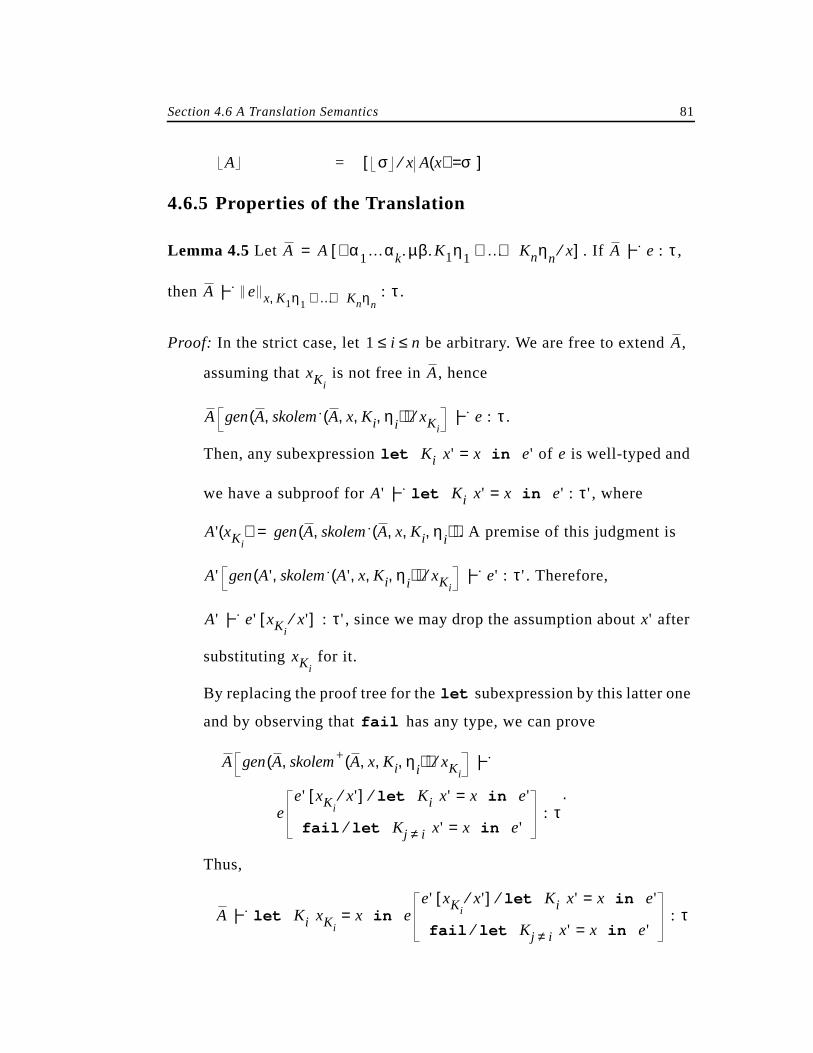
Section 4.6 A Translation Semantics 81
=
4.6.5 Properties of the Translation
Lemma 4.5Let . If ,
then .
Proof: In the strict case, let be arbitrary. We are free to extend ,
assuming that is not free in , hence
.
Then, any subexpression of is well-typed and
we have a subproof for , where
. A premise of this judgment is
. Therefore,
, since we may drop the assumption about after
substituting for it.
By replacing the proof tree for the subexpression by this latter one
and by observing that has any type, we can prove
.
Thus,
A σ x⁄ A x( ) σ=[ ]
A A α1…αk.∀ µβ.K1η1 … Knηn+ + x⁄[ ]= A |−. e : τ
A |−. e x K1η1 … Knηn+ +, : τ
1 i n≤ ≤ A
xKiA
A gen A skolem. A x Ki ηi, , ,( ),( ) xKi⁄ |−. e : τ
let Ki x' x= in e' e
A' |−.let Ki x' x= in e' : τ'
A' xKi( ) gen A skolem. A x Ki ηi, , ,( ),( )=
A' gen A' skolem. A' x Ki ηi, , ,( ),( ) xKi⁄ |−. e' : τ'
A' |−. e' xKix'⁄[ ] : τ' x'
xKi
let
fail
A gen A skolem+ A x Ki ηi, , ,( ),( ) xKi⁄ |−.
ee' xKi
x'⁄[ ] let Ki x' x= in e'⁄
fail let Kj i≠ x' x= in e'⁄: τ
A |−.let Ki xKi
x= in ee' xKi
x'⁄[ ] let Ki x' x= in e'⁄
fail let Kj i≠ x' x= in e'⁄: τ
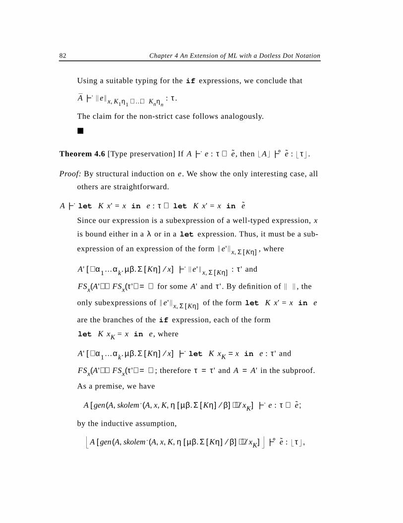
82 Chapter 4 An Extension of ML with a Dotless Dot Notation
Using a suitable typing for the expressions, we conclude that
.
The claim for the non-strict case follows analogously.
Theorem 4.6[Type preservation] If , then .
Proof: By structural induction on . We show the only interesting case, all
others are straightforward.
Since our expression is a subexpression of a well-typed expression,
is bound either in a or in a expression. Thus, it must be a sub-
expression of an expression of the form , where
and
for some and . By definition of , the
only subexpressions of of the form
are the branches of the expression, each of the form
, where
and
; therefore and in the subproof.
As a premise, we have
;
by the inductive assumption,
,
if
A |−. e x K1η1 … Knηn+ +, : τ
A |−. e : τ e⇒ A |−° e : τ
e
A |−.let K x' = x in e : τ let K x' = x in e⇒
x
λ let
e' x Σ Kη[ ],
A' α1…αk.∀ µβ.Σ Kη[ ] x⁄[ ] |−. e' x Σ Kη[ ], : τ'
FSx A'( ) FSx τ'( )∪ ∅= A' τ'
e' x Σ Kη[ ], let K x' = x in e
if
let K xK = x in e
A' α1…αk.∀ µβ.Σ Kη[ ] x⁄[ ] |−.let K xK x= in e : τ'
FSx A'( ) FSx τ'( )∪ ∅= τ τ'= A A'=
A gen A skolem. A x K η µβ.Σ Kη[ ] β⁄[ ], , ,( ),( ) xK⁄[ ] |−. e : τ e⇒
A gen A skolem. A x K η µβ.Σ Kη[ ] β⁄[ ], , ,( ),( ) xK⁄[ ] |−° e : τ
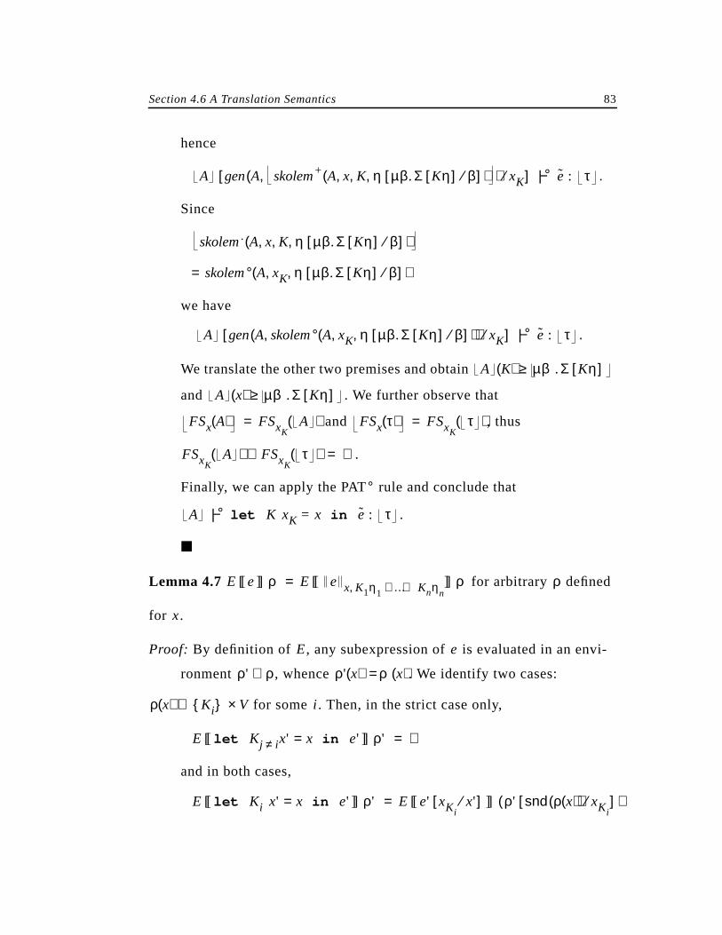
Section 4.6 A Translation Semantics 83
hence
.
Since
=
we have
.
We translate the other two premises and obtain
and . We further observe that
and , thus
.
Finally, we can apply the PAT rule and conclude that
.
Lemma 4.7 for arbitrary defined
for .
Proof: By definition of , any subexpression of is evaluated in an envi-
ronment , whence . We identify two cases:
for some . Then, in the strict case only,
and in both cases,
A gen A skolem+ A x K η µβ.Σ Kη[ ] β⁄[ ], , ,( ),( ) xK⁄[ ] |−° e : τ
skolem. A x K η µβ.Σ Kη[ ] β⁄[ ], , ,( )
skolem° A xK η µβ.Σ Kη[ ] β⁄[ ], ,( )
A gen A skolem° A xK η µβ.Σ Kη[ ] β⁄[ ], ,( ),( ) xK⁄[ ] |−° e : τ
A K( ) µβ.Σ Kη[ ]≥
A x( ) µβ.Σ Kη[ ]≥
FSx A( ) FSxKA( )= FSx τ( ) FSxK
τ( )=
FSxKA( ) FSxK
τ( )∪ ∅=
°
A |−° let K xK = x in e : τ
E [[ e]] ρ E [[ e x K1η1 … Knηn+ +, ]] ρ= ρ
x
E e
ρ' ρ⊇ ρ' x( ) ρ x( )=
ρ x( ) Ki V×∈ i
E [[ let Kj i≠ x' x= in e' ]] ρ' ⊥=
E [[ let Ki x' x= in e' ]] ρ' E [[ e' xKix'⁄[ ] ]] ρ' snd ρ x( )( ) xKi
⁄[ ]( )=
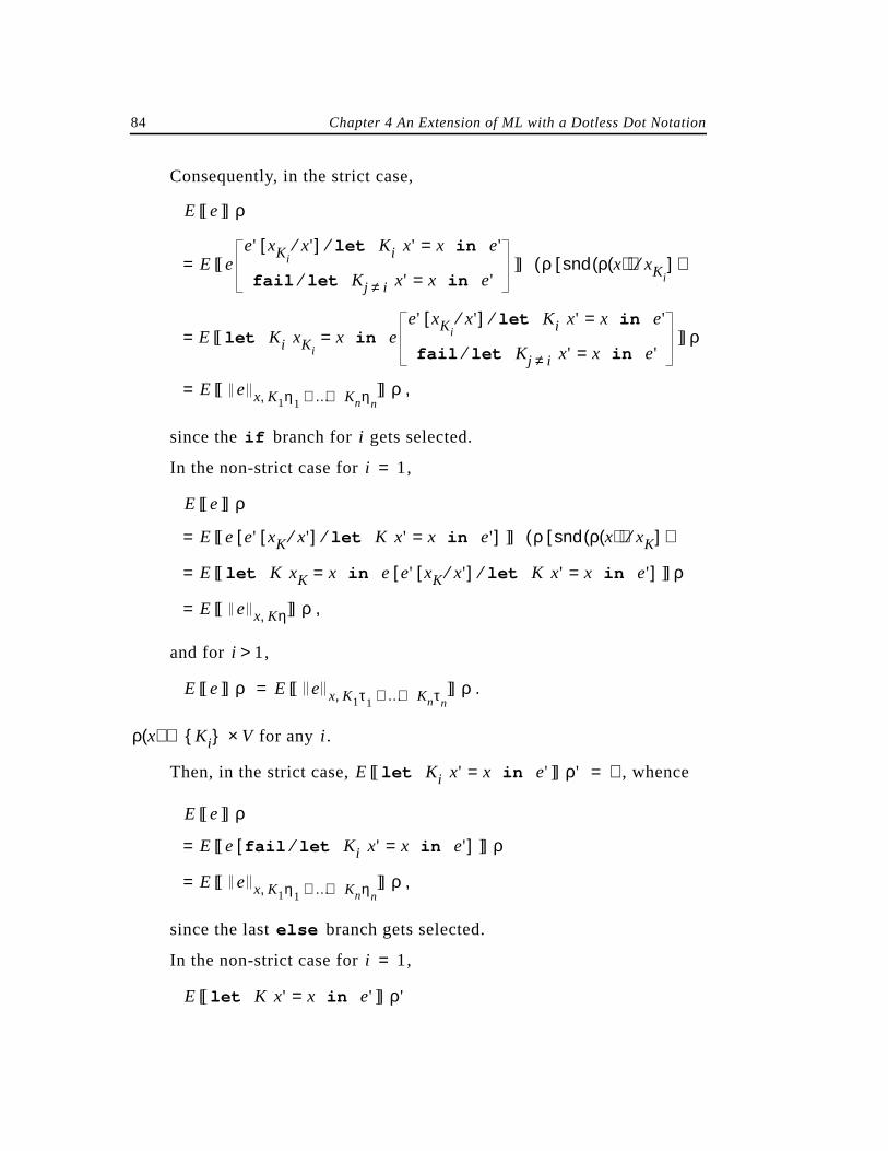
84 Chapter 4 An Extension of ML with a Dotless Dot Notation
Consequently, in the strict case,
=
=
= ,
since the branch for gets selected.
In the non-strict case for ,
=
=
= ,
and for ,
.
for any .
Then, in the strict case, , whence
=
= ,
since the last branch gets selected.
In the non-strict case for ,
E [[ e]] ρ
E [[ ee' xKi
x'⁄[ ] let Ki x' x= in e'⁄
fail let Kj i≠ x' x= in e'⁄]] ρ snd ρ x( )( ) xKi
⁄[ ]( )
E [[ let Ki xKix= in e
e' xKix'⁄[ ] let Ki x' x= in e'⁄
fail let Kj i≠ x' x= in e'⁄]] ρ
E [[ e x K1η1 … Knηn+ +, ]] ρ
if i
i 1=
E [[ e]] ρ
E [[ e e' xK x'⁄[ ] let K x' x= in e'⁄[ ] ]] ρ snd ρ x( )( ) xK⁄[ ]( )
E [[ let K xK x= in e e' xK x'⁄[ ] let K x' x= in e'⁄[ ] ]] ρ
E [[ e x Kη, ]] ρ
i 1>
E [[ e]] ρ E [[ e x K1τ1 … Knτn+ +, ]] ρ=
ρ x( ) Ki V×∉ i
E [[ let Ki x' x= in e' ]] ρ' ⊥=
E [[ e]] ρ
E [[ e fail let Ki x' x= in e'⁄[ ] ]] ρ
E [[ e x K1η1 … Knηn+ +, ]] ρ
else
i 1=
E [[ let K x' x= in e' ]] ρ'
Section 4.6 A Translation Semantics 85
=
= .
Therefore,
=
= .
Theorem 4.8[Preservation of semantics] If , then
for arbitrary .
Proof: By structural induction on .
Corollary 4.9 [Semantic soundness] If is a closed term, and
as defined previously, then .
Proof: Follows immediately from the two theorems, observing that
and , since neither nor contain any ’s.
E [[ e' ]] ρ' ⊥ x'⁄[ ]( )
E [[ e' xK x'⁄[ ] ]] ρ' ⊥ xK⁄[ ]( )
E [[ e]] ρ
E [[ e e' xK x'⁄[ ] let K x' x= in e'⁄[ ] ]] ρ ⊥ xK⁄[ ]( )
E [[ e x Kη, ]] ρ
A |−. e : τ e⇒
E [[ e]] ρ E [[ e]] ρ= ρ
e
e A |−. e : τ
|= ρ ψ, A E [[ e]] ρ T [[ τ ]] ψ∈
τ τ=
A A= τ A κ
86
5 An Extension of Haskell withFirst-Class Abstract Types
This chapter introduces an extension of the functional language Haskell
with existential types. Existential types combine well with the systematic
overloading polymorphism provided by Haskell type classes. Briefly, we ex-
tend Haskell’sdata declaration in a similar way as the ML datatype decla-
ration above. In Haskell, it is possible to specify what type class a (univer-
sally quantified) type variable belongs to. In our extension, we can do the
same for existentially quantified type variables. This lets us use type classes
as signatures of abstract data types; we can then construct heterogeneous ag-
gregates over a given type class. A type reconstruction algorithm is given,
and semantic soundness is shown by translating into an extension of the lan-
guage from Chapter 3.
5.1 Introduction
Haskell [HPJW+92] uses type classes as a systematic approach to ad-hoc
polymorphism, otherwise known as overloading. Type classes capture com-
mon sets of operations. A particular type may be an instance of a type class,
and has an operation corresponding to each operation defined in the type
class. Type classes may be arranged hierarchically.
Section 5.1 Introduction 87
In [WB89], Wadler and Blott called for a closer exploration of the rela-
tionship between type classes and abstract data types. After an initial explo-
ration described in [LO91], we now present an extension of Haskell with
datatypes whose component types may be existentially quantified.
In Haskell, an algebraic datatype declaration is of the form
data = | |
It introduces a new type constructor with value constructors .
The optional context specifies of which type classes the type variables
are instances. The constructors are used in two ways: as functions
to construct values, and in patterns to decompose values already construct-
ed. The types of the constructors are universally quantified over the type
variables ; no other type variable may appear free in the component
types .
We describe an extension of Haskell analogous to the extension of ML
described above. Type variables that appear free in the component types are
interpreted as existentially quantified. In addition to the “global” context for
the universally quantified parameters of the type constructor, we introduce
“local” contexts for each value constructor. The local context specifies of
which type classes the existentially quantified type variables in the compo-
nent types are instances. The extended datatype declaration is of the form
data =
|
|
When constructing a value using a constructor with an existentially quanti-
fied component type, the existential type variables instantiate to the actual
types of the corresponding function arguments, and we lose any information
on the actual types. However, we know that these types are instances of the
same type classes as the corresponding existential type variables. This
c ⇒[ ] T a1…an K1 t11…t1k1… Km tm1…tmkm
T K1 … Km, ,
c
a1 … an, ,
a1 … an, ,
tij
c ⇒[ ] T a1…an c1 ⇒[ ] K1 t11…t1k1
…cm ⇒[ ] Km tm1…tmkm
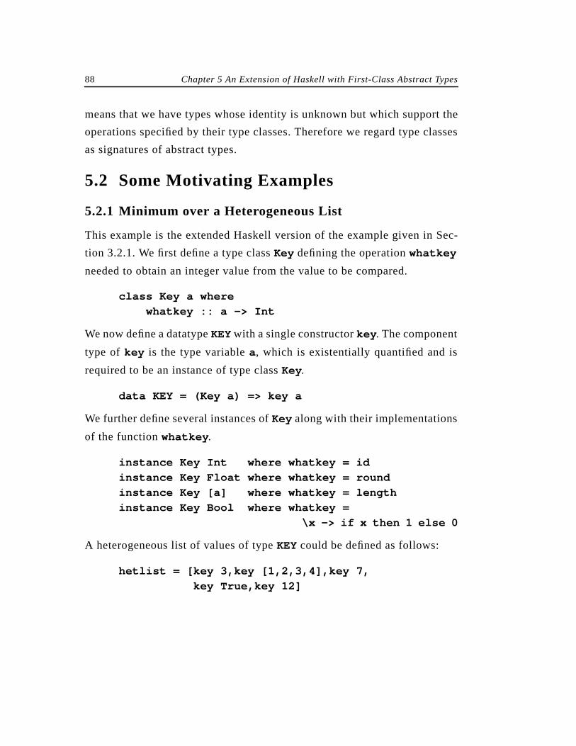
88 Chapter 5 An Extension of Haskell with First-Class Abstract Types
means that we have types whose identity is unknown but which support the
operations specified by their type classes. Therefore we regard type classes
as signatures of abstract types.
5.2 Some Motivating Examples
5.2.1 Minimum over a Heterogeneous List
This example is the extended Haskell version of the example given in Sec-
tion 3.2.1. We first define a type classKey defining the operationwhatkey
needed to obtain an integer value from the value to be compared.
class Key a where
whatkey :: a -> Int
We now define a datatypeKEY with a single constructorkey . The component
type of key is the type variablea, which is existentially quantified and is
required to be an instance of type classKey.
data KEY = (Key a) => key a
We further define several instances ofKey along with their implementations
of the functionwhatkey .
instance Key Int where whatkey = id
instance Key Float where whatkey = round
instance Key [a] where whatkey = length
instance Key Bool where whatkey =
\x -> if x then 1 else 0
A heterogeneous list of values of typeKEY could be defined as follows:
hetlist = [key 3,key [1,2,3,4],key 7,
key True,key 12]
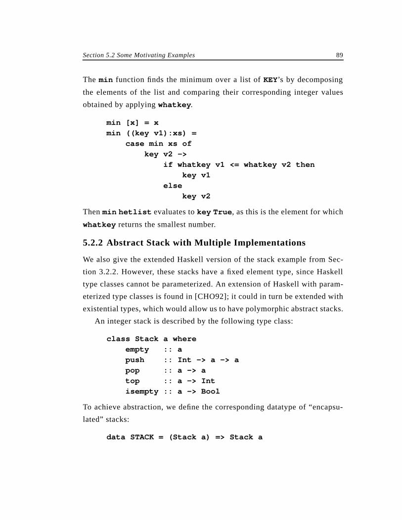
Section 5.2 Some Motivating Examples 89
The min function finds the minimum over a list ofKEY’s by decomposing
the elements of the list and comparing their corresponding integer values
obtained by applyingwhatkey .
min [x] = x
min ((key v1):xs) =
case min xs of
key v2 ->
if whatkey v1 <= whatkey v2 then
key v1
else
key v2
Thenmin hetlist evaluates tokey True , as this is the element for which
whatkey returns the smallest number.
5.2.2 Abstract Stack with Multiple Implementations
We also give the extended Haskell version of the stack example from Sec-
tion 3.2.2. However, these stacks have a fixed element type, since Haskell
type classes cannot be parameterized. An extension of Haskell with param-
eterized type classes is found in [CHO92]; it could in turn be extended with
existential types, which would allow us to have polymorphic abstract stacks.
An integer stack is described by the following type class:
class Stack a where
empty :: a
push :: Int -> a -> a
pop :: a -> a
top :: a -> Int
isempty :: a -> Bool
To achieve abstraction, we define the corresponding datatype of “encapsu-
lated” stacks:
data STACK = (Stack a) => Stack a
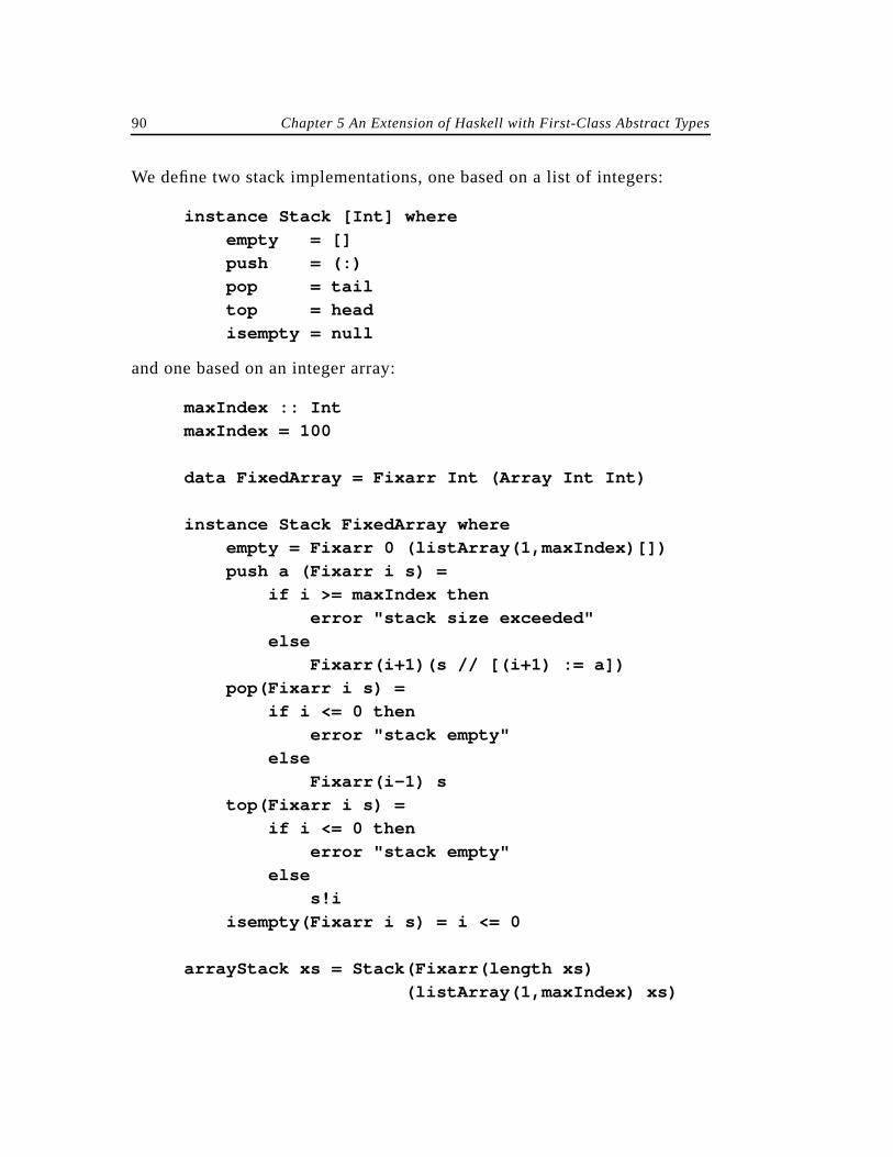
90 Chapter 5 An Extension of Haskell with First-Class Abstract Types
We define two stack implementations, one based on a list of integers:
instance Stack [Int] where
empty = []
push = (:)
pop = tail
top = head
isempty = null
and one based on an integer array:
maxIndex :: Int
maxIndex = 100
data FixedArray = Fixarr Int (Array Int Int)
instance Stack FixedArray where
empty = Fixarr 0 (listArray(1,maxIndex)[])
push a (Fixarr i s) =
if i >= maxIndex then
error "stack size exceeded"
else
Fixarr(i+1)(s // [(i+1) := a])
pop(Fixarr i s) =
if i <= 0 then
error "stack empty"
else
Fixarr(i-1) s
top(Fixarr i s) =
if i <= 0 then
error "stack empty"
else
s!i
isempty(Fixarr i s) = i <= 0
arrayStack xs = Stack(Fixarr(length xs)
(listArray(1,maxIndex) xs)
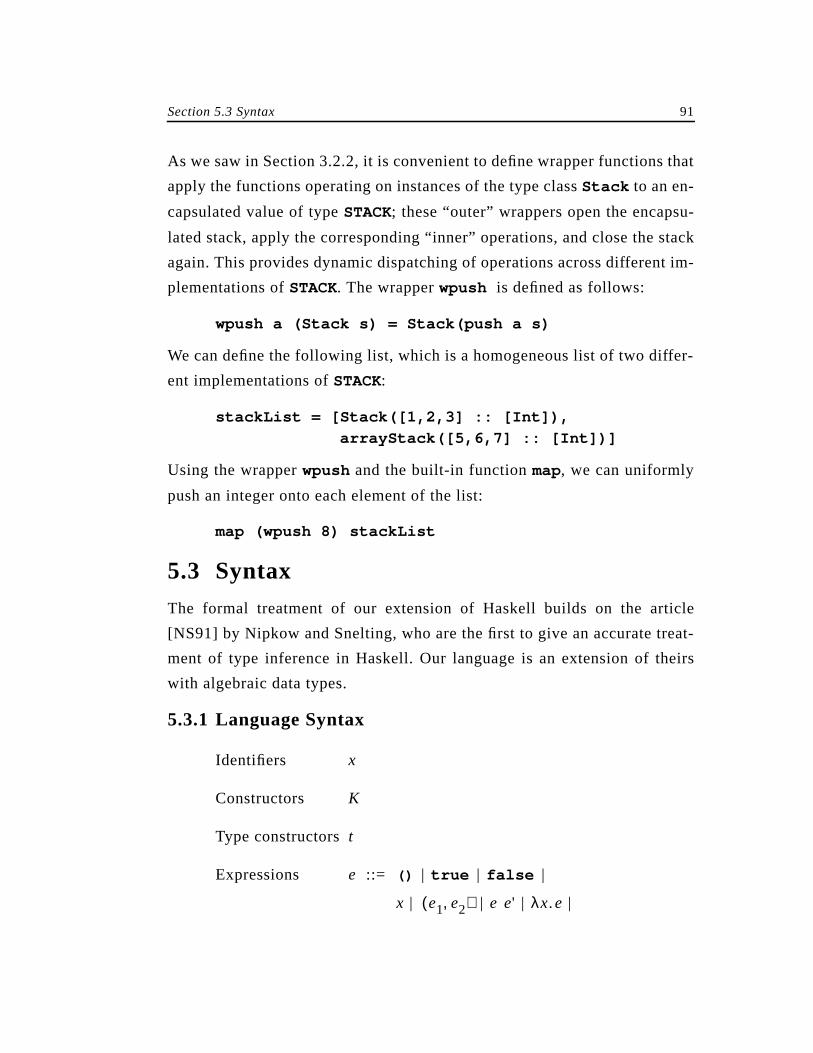
Section 5.3 Syntax 91
As we saw in Section 3.2.2, it is convenient to define wrapper functions that
apply the functions operating on instances of the type classStack to an en-
capsulated value of typeSTACK; these “outer” wrappers open the encapsu-
lated stack, apply the corresponding “inner” operations, and close the stack
again. This provides dynamic dispatching of operations across different im-
plementations ofSTACK. The wrapperwpush is defined as follows:
wpush a (Stack s) = Stack(push a s)
We can define the following list, which is a homogeneous list of two differ-
ent implementations ofSTACK:
stackList = [Stack([1,2,3] :: [Int]),
arrayStack([5,6,7] :: [Int])]
Using the wrapperwpush and the built-in functionmap, we can uniformly
push an integer onto each element of the list:
map (wpush 8) stackList
5.3 Syntax
The formal treatment of our extension of Haskell builds on the article
[NS91] by Nipkow and Snelting, who are the first to give an accurate treat-
ment of type inference in Haskell. Our language is an extension of theirs
with algebraic data types.
5.3.1 Language Syntax
Identifiers
Constructors
Type constructors
Expressions ::= | | |
| | | |
x
K
t
e () true false
x e1 e2,( ) e e' λx.e
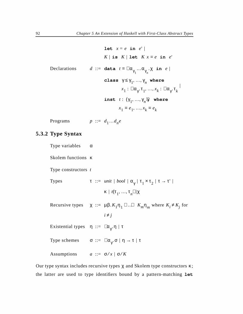
92 Chapter 5 An Extension of Haskell with First-Class Abstract Types
|
| |
Declarations ::= |
|
Programs ::=
5.3.2 Type Syntax
Type variables
Skolem functions
Type constructors
Types ::= | | | | |
| |
Recursive types ::= where for
Existential types ::= |
Type schemes ::= | |
Assumptions ::= |
Our type syntax includes recursive types and Skolem type constructors ;
the latter are used to type identifiers bound by a pattern-matchinglet
let x = e in e'
K is K let K x e= in e'
d data t αγ1…αγn
.∀ χ= in e
class γ γ1 … γn, ,≤ where
x1 : αγ.∀ τ1 … xk : αγ.∀ τk, ,
inst t : γ1 … γn, ,( ) γ where
x1 e1= … xk ek=, ,
p d1…dne
α
κ
t
τ unit bool αγ τ1 τ2× τ τ'→
κ t τ1 … τn, ,( ) χ
χ µβ.K1η1 … Kmηm+ + Ki Kj≠
i j≠
η αγ.η∃ τ
σ αγ.σ∀ η τ→ τ
a σ x⁄ σ K⁄
χ κ
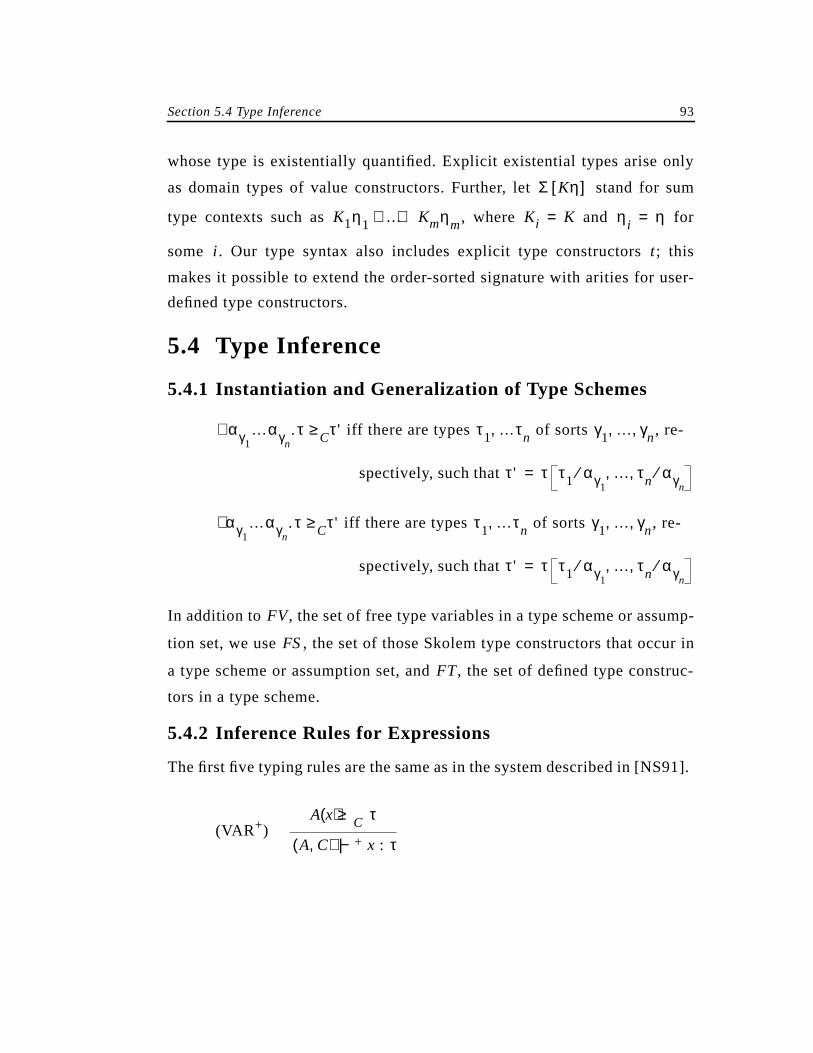
Section 5.4 Type Inference 93
whose type is existentially quantified. Explicit existential types arise only
as domain types of value constructors. Further, let stand for sum
type contexts such as , where and for
some . Our type syntax also includes explicit type constructors ; this
makes it possible to extend the order-sorted signature with arities for user-
defined type constructors.
5.4 Type Inference
5.4.1 Instantiation and Generalization of Type Schemes
iff there are types of sorts , re-
spectively, such that
iff there are types of sorts , re-
spectively, such that
In addition to , the set of free type variables in a type scheme or assump-
tion set, we use , the set of those Skolem type constructors that occur in
a type scheme or assumption set, and , the set of defined type construc-
tors in a type scheme.
5.4.2 Inference Rules for Expressions
The first five typing rules are the same as in the system described in [NS91].
(VAR+)
Σ Kη[ ]
K1η1 … Kmηm+ + Ki K= ηi η=
i t
αγ1…αγn
.τ∀ ≥ Cτ' τ1 …τn, γ1 … γn, ,
τ' τ τ1 αγ1⁄ … τn αγn
⁄, ,=
αγ1…αγn
.τ∃ ≥ Cτ' τ1 …τn, γ1 … γn, ,
τ' τ τ1 αγ1⁄ … τn αγn
⁄, ,=
FV
FS
FT
A x( ) ≥C τ
A C,( ) |−+ x : τ
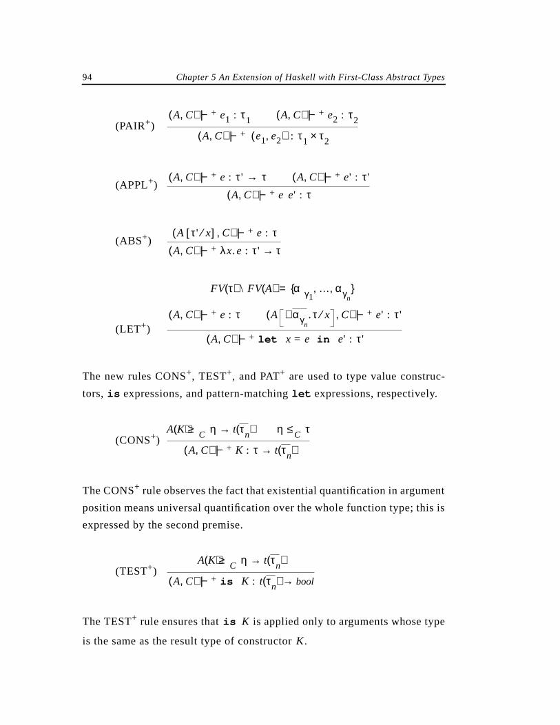
94 Chapter 5 An Extension of Haskell with First-Class Abstract Types
(PAIR+)
(APPL+)
(ABS+)
(LET+)
The new rules CONS+, TEST+, and PAT+ are used to type value construc-
tors, is expressions, and pattern-matchinglet expressions, respectively.
(CONS+)
The CONS+ rule observes the fact that existential quantification in argument
position means universal quantification over the whole function type; this is
expressed by the second premise.
(TEST+)
The TEST+ rule ensures that is applied only to arguments whose type
is the same as the result type of constructor .
A C,( ) |−+ e1 : τ1 A C,( ) |−+ e2 : τ2
A C,( ) |−+ e1 e2,( ) : τ1 τ2×
A C,( ) |−+ e : τ' → τ A C,( ) |−+ e' : τ'
A C,( ) |−+ e e' : τ
A τ' x⁄[ ] C,( ) |−+ e : τA C,( ) |−+ λx.e : τ' τ→
FV τ( ) \ FV A( ) αγ1… αγn
, , =
A C,( ) |−+ e : τ A αγn.∀ τ x⁄ C,( ) |−+ e' : τ'
A C,( ) |−+ let x = e in e' : τ'
A K( ) ≥ C η t τn( )→ η ≤ C τ
A C,( ) |−+ K : τ t τn( )→
A K( ) ≥ C η t τn( )→
A C,( ) |−+ is K : t τn( ) bool→
is K
K
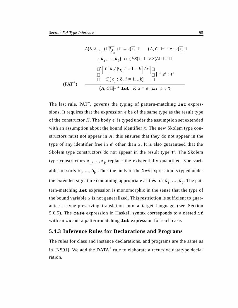
Section 5.4 Type Inference 95
(PAT+)
The last rule, PAT+, governs the typing of pattern-matchinglet expres-
sions. It requires that the expression be of the same type as the result type
of the constructor . The body is typed under the assumption set extended
with an assumption about the bound identifier . The new Skolem type con-
structors must not appear in ; this ensures that they do not appear in the
type of any identifier free in other than . It is also guaranteed that the
Skolem type constructors do not appear in the result type . The Skolem
type constructors replace the existentially quantified type vari-
ables of sorts . Thus the body of thelet expression is typed under
the extended signature containing appropriate arities for . The pat-
tern-matchinglet expression is monomorphic in the sense that the type of
the bound variable is not generalized. This restriction is sufficient to guar-
antee a type-preserving translation into a target language (see Section
5.6.5). Thecase expression in Haskell syntax corresponds to a nestedif
with an is and a pattern-matchinglet expression for each case.
5.4.3 Inference Rules for Declarations and Programs
The rules for class and instance declarations, and programs are the same as
in [NS91]. We add the DATA+ rule to elaborate a recursive datatype decla-
ration.
A K( ) ≥ C βδk.∃ τ( ) t τn( )→ A C,( ) |−+ e : t τn( )
κ1 … κk, , FS τ'( ) FS A( )∪( )∩ ∅=
A τ κi βδi⁄ i 1…k= x⁄
C κi : δi i 1…k=[ ]
|−+ e' : τ'
A C,( ) |−+ let K x = e in e' : τ'
e
K e'
x
A
e' x
τ'
κ1 … κk, ,
δ1 … δk, ,
κ1 … κk, ,
x
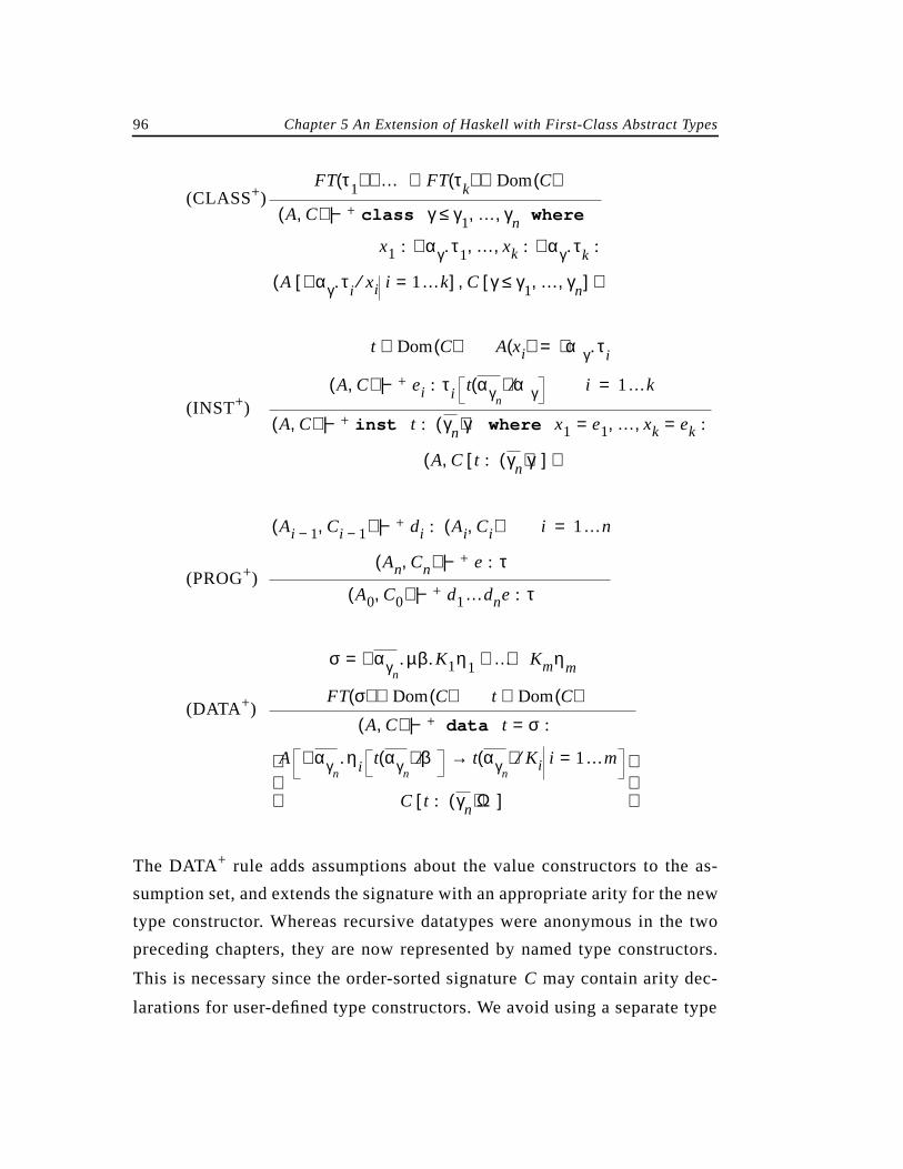
96 Chapter 5 An Extension of Haskell with First-Class Abstract Types
(CLASS+)
(INST+)
(PROG+)
(DATA +)
The DATA+ rule adds assumptions about the value constructors to the as-
sumption set, and extends the signature with an appropriate arity for the new
type constructor. Whereas recursive datatypes were anonymous in the two
preceding chapters, they are now represented by named type constructors.
This is necessary since the order-sorted signature may contain arity dec-
larations for user-defined type constructors. We avoid using a separate type
FT τ1( ) … FT τk( )∪ ∪ Dom C( )⊆
A C,( ) |−+ class γ γ1 … γn, ,≤ where
x1 : αγ.∀ τ1 … xk : αγ.∀ τk, , :
A αγ.∀ τi xi⁄ i 1…k=[ ] C γ γ1 … γn, ,≤[ ],( )
t Dom C( )∈ A xi( ) αγ.∀ τi=
A C,( ) |−+ ei : τi t αγn( ) αγ⁄ i 1…k=
A C,( ) |−+ inst t : γn( ) γ where x1 e1= … xk ek=, , :
A C t : γn( ) γ[ ],( )
Ai 1− Ci 1−,( ) |−+ di : Ai Ci,( ) i 1…n=
An Cn,( ) |−+ e : τ
A0 C0,( ) |−+ d1…dne : τ
σ αγn.∀ µβ.K1η1 … Kmηm+ +=
FT σ( ) Dom C( )⊆ t Dom C( )∉A C,( ) |−+ data t σ= :
A αγn.∀ ηi t αγn
( ) β⁄ t αγn( )→ Ki⁄ i 1…m=
C t : γn( ) Ω[ ]
C
Section 5.5 Type Reconstruction 97
constructor environment; therefore, in an assumption about a value
constructor, now is the type scheme for when regarded as a function, as
opposed to the type scheme describing the entire recursive datatype be-
longs to.
5.4.4 Relation to the Haskell Type Inference System
Theorem 5.1[Conservative extension] Let Mini-Haskell’ be an extension
of Mini-Haskell with recursive datatypes and a monomorphic pattern-
matchinglet expression, but without existential quantification. Then, for
any Mini-Haskell’ program , iff .
Proof: By structural induction on .
Corollary 5.2 [Conservative extension] Our type system is a conservative
extension of the Mini-Haskell type system described in [NS91], in the fol-
lowing sense: For any Mini-Haskell program , iff
.
Proof: Follows immediately from Theorem 5.1.
5.5 Type Reconstruction
The type reconstruction algorithm is a translation from the deterministic
typing rules, using order-sorted unification [SS85][MGS89] instead of stan-
dard unification.
5.5.1 Unitary Signatures for Principal Types
The article [NS91] describes several conditions necessary to guarantee uni-
tary signatures, which are sufficient to guarantee principal types. First, to
make a signature regular and downward compete, we perform the follow-
ing two steps to obtain a new signature :
σ K⁄
σ K
K
p A C,( ) |−+ p : τ A C,( ) |− MH' p : τ
p
p A C,( ) |−+ p : τ
A C,( ) |− MH p : τ
C
CR
98 Chapter 5 An Extension of Haskell with First-Class Abstract Types
• For any two incomparable classes , we introduce a new
class declaration with an empty part combin-
ing the operations of and .
• Then, for each type constructor with instance declarations
introduce another instance declaration of the form
where is simply the additionally declared class if and are in-
comparable, or otherwise the lower one in the class hierarchy.
Note that Haskell uses multiple class assertions for type variables to express
this conjunction of classes.
Since regular signatures alone do not guarantee the existence of principal
types, we impose the following two conditions on , which are also
present in Haskell:
• Injectivity: A type constructor may not be declared as an instance of a
particular class more than once in the same scope
• Subsort reflection: If are the immediate superclasses of , a
declaration must be preceded by declara-
tions such that is a subclass of for
al and .
As discussed in [NS91], a Haskell signature that satisfies these conditions is
unitary.
γ1 γ2, Dom C( )∈
class γ γ1 γ2,≤ where
γ1 γ2
inst t : γ1n( ) γ1 where …
inst t : γ2n( ) γ2 where …
inst t : γ11 γ21∧ … γ1n γ2n∧, ,( ) γ1 γ2∧( )
γ δ∧ γ δ
CR
γ1 … γm, , δ
inst t : δn( ) δ where …
inst t : γni( ) γi where … δj γj
i
i 1…m= j 1…n=
Section 5.5 Type Reconstruction 99
5.5.2 Auxiliary Functions
In our algorithm, we need to instantiate universally quantified types and
generalize existentially quantified types. Both are handled in the same way.
where are
fresh type variables
where are
fresh type variables
the most general unifier of and under order-
sorted signature
5.5.3 Algorithm
Our type reconstruction function takes an assumption set, an order-sorted
signature, and an expression, and it returns a substitution and a type expres-
sion. There is one case for each typing rule.
inst∀ αγ1…αγn
.∀ τ( ) τ βγ1αγ1
⁄ … βγnαγn
⁄, ,= βγn… βγn
, ,
inst∃ αγ1…αγn
.∃ τ( ) τ βγ1αγ1
⁄ … βγnαγn
⁄, ,= βγn… βγn
, ,
osuC τ τ',( ) τ τ'
C
TE A C x, ,( ) =
Id inst∀ A x( )( ),( )
TE A C e1 e2,( ), ,( ) =
let S1 τ1,( ) = TE A C e1, ,( )
S2 τ2,( ) = TE S1A C e2, ,( )
in S2S1 S2τ1 τ2×,( )
100 Chapter 5 An Extension of Haskell with First-Class Abstract Types
TE A C ee', ,( ) =
let S τ,( ) = TE A C e, ,( )S' τ',( ) = TE SA C e', ,( )
β be a fresh type variable
U = osuC S'τ τ' β→,( )
in US'S Uβ,( )
TE A C λx.e, ,( ) =
let β be a fresh type variable
S τ,( ) = TE A β x⁄[ ] C e, ,( )in
S Sβ τ→,( )
TE A C let x = e in e', ,( ) =
let S τ,( ) = TE A C e, ,( )S' τ',( ) = TE SA gen SAτ,( ) x⁄[ ] C e', ,( )
in
S'S τ',( )
TE A C K, ,( ) =
let η τ→ inst∀ A K( )( )=
in Id inst∃ η( )( ) τ→,( )
TE A C is K, ,( ) =
let η τ→ inst∀ A K( )( )=
in Id τ bool→,( )
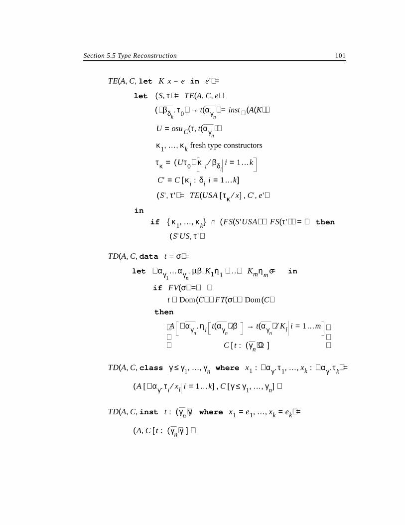
Section 5.5 Type Reconstruction 101
TE A C let K x = e in e', ,( ) =
let S τ,( ) = TE A C e, ,( )
βδk.∃ τ0( ) t αγn
( )→ = inst∀ A K( )( )
U osuC τ t αγn( ),( )=
κ1 … κk, , fresh type constructors
τκ Uτ0( ) κi βδi⁄ i 1…k==
C' C κi : δi i 1…k=[ ]=
S' τ',( ) = TE USA τκ x⁄[ ] C' e', ,( )
in
if κ1 … κk, , FS S'USA( ) FS τ'( )∪( )∩ ∅= then
S'US τ',( )
TD A C data t σ=, ,( ) =
let αγ1…αγn
.∀ µβ.K1η1 … Kmηm+ + σ= in
if FV σ( ) ∅= ∧t Dom C( )∉ FT σ( ) Dom C( )⊆∧
then
A αγn.∀ ηi t αγn
( ) β⁄ t αγn( )→ Ki⁄ i 1…m=
C t : γn( ) Ω[ ]
TD A C class γ γ1 … γn, ,≤ where x1 : αγ.∀ τ1 … xk : αγ.∀ τk, ,, ,( ) =
A αγ.∀ τi xi⁄ i 1…k=[ ] C γ γ1 … γn, ,≤[ ],( )
TD A C inst t : γn( ) γ where x1 e1= … xk ek=, ,, ,( ) =
A C t : γn( ) γ[ ],( )
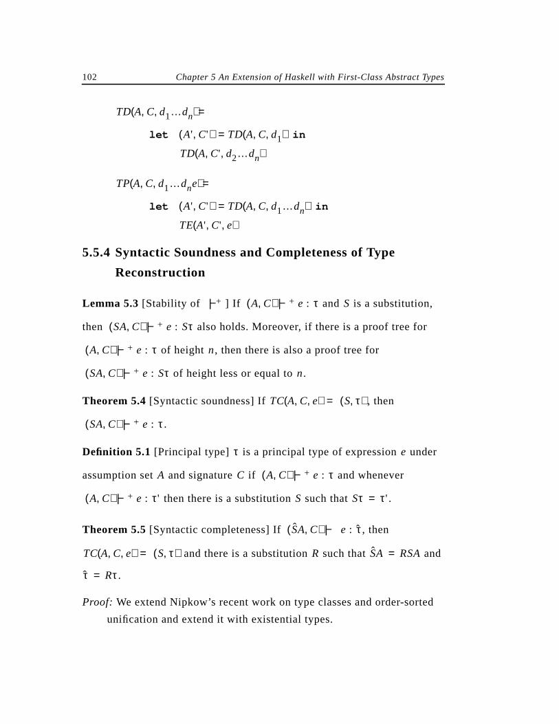
102 Chapter 5 An Extension of Haskell with First-Class Abstract Types
5.5.4 Syntactic Soundness and Completeness of Type
Reconstruction
Lemma 5.3 [Stability of ] If and is a substitution,
then also holds. Moreover, if there is a proof tree for
of height , then there is also a proof tree for
of height less or equal to .
Theorem 5.4[Syntactic soundness] If , then
.
Definition 5.1 [Principal type] is a principal type of expression under
assumption set and signature if and whenever
then there is a substitution such that .
Theorem 5.5[Syntactic completeness] If , then
and there is a substitution such that and
.
Proof: We extend Nipkow’s recent work on type classes and order-sorted
unification and extend it with existential types.
TD A C d1…dn, ,( ) =
let A' C',( ) TD A C d1, ,( )= in
TD A C' d2…dn, ,( )
TP A C d1…dne, ,( ) =
let A' C',( ) TD A C d1…dn, ,( )= in
TE A' C' e, ,( )
|−+ A C,( ) |−+ e : τ S
SA C,( ) |−+ e : Sτ
A C,( ) |−+ e : τ n
SA C,( ) |−+ e : Sτ n
TC A C e, ,( ) S τ,( )=
SA C,( ) |−+ e : τ
τ e
A C A C,( ) |−+ e : τ
A C,( ) |−+ e : τ' S Sτ τ'=
SA C,( ) |− e : τ
TC A C e, ,( ) S τ,( )= R SA RSA=
τ Rτ=
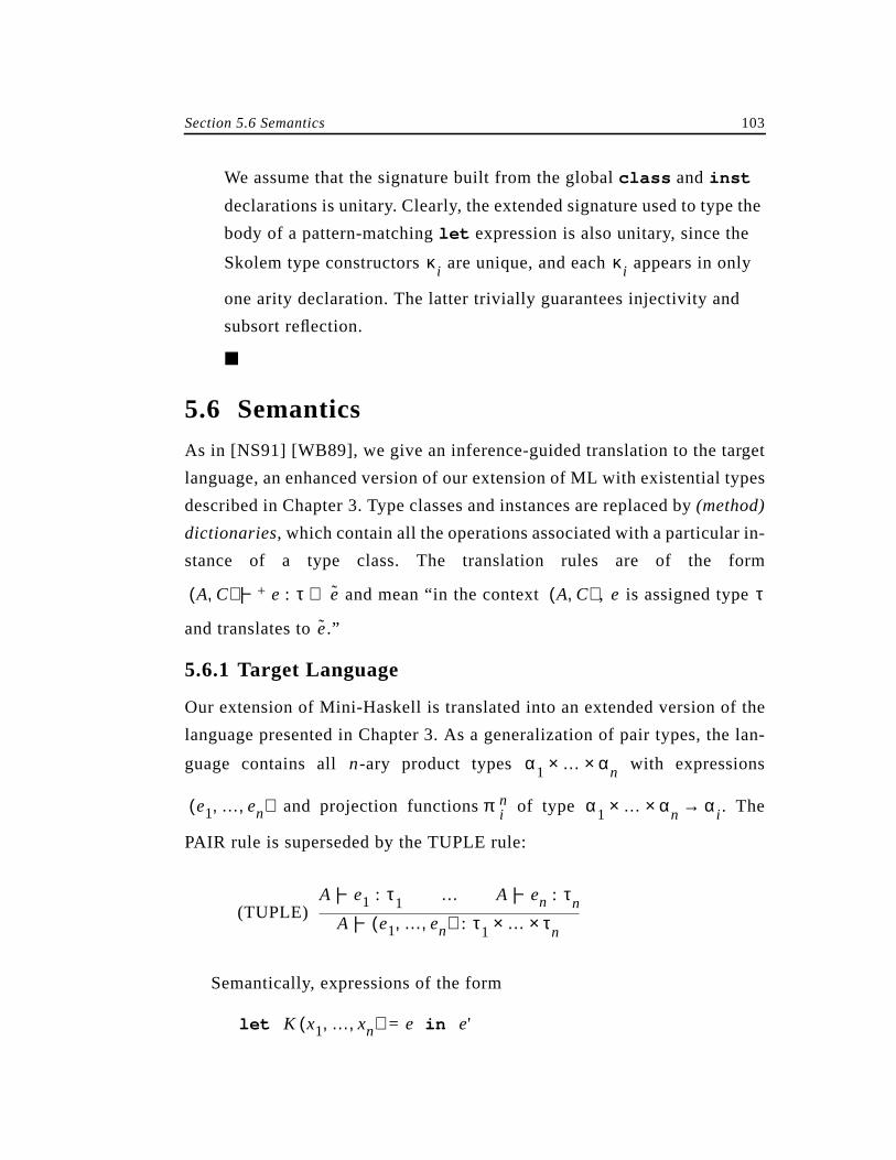
Section 5.6 Semantics 103
We assume that the signature built from the globalclass and inst
declarations is unitary. Clearly, the extended signature used to type the
body of a pattern-matchinglet expression is also unitary, since the
Skolem type constructors are unique, and each appears in only
one arity declaration. The latter trivially guarantees injectivity and
subsort reflection.
5.6 Semantics
As in [NS91] [WB89], we give an inference-guided translation to the target
language, an enhanced version of our extension of ML with existential types
described in Chapter 3. Type classes and instances are replaced by(method)
dictionaries, which contain all the operations associated with a particular in-
stance of a type class. The translation rules are of the form
and mean “in the context , is assigned type
and translates to .”
5.6.1 Target Language
Our extension of Mini-Haskell is translated into an extended version of the
language presented in Chapter 3. As a generalization of pair types, the lan-
guage contains all -ary product types with expressions
and projection functions of type . The
PAIR rule is superseded by the TUPLE rule:
(TUPLE)
Semantically, expressions of the form
κi κi
A C,( ) |−+ e : τ e⇒ A C,( ) e τ
e
n α1 … αn××
e1 … en, ,( ) πin α1 … αn×× αi→
A |− e1 : τ1 … A |− en : τn
A |− e1 … en, ,( ) : τ1 … τn××
let K x1 … xn, ,( ) = e in e'
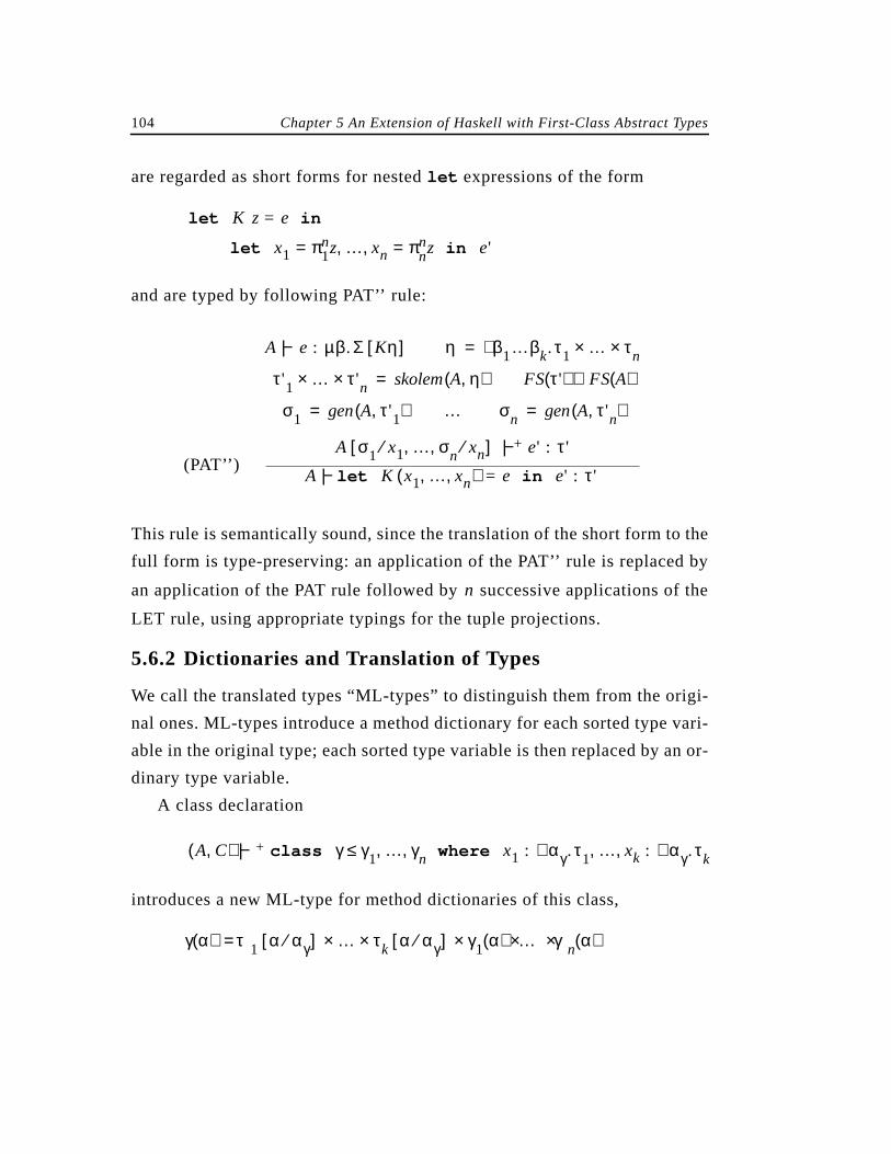
104 Chapter 5 An Extension of Haskell with First-Class Abstract Types
are regarded as short forms for nestedlet expressions of the form
and are typed by following PAT’’ rule:
(PAT’’)
This rule is semantically sound, since the translation of the short form to the
full form is type-preserving: an application of the PAT’’ rule is replaced by
an application of the PAT rule followed by successive applications of the
LET rule, using appropriate typings for the tuple projections.
5.6.2 Dictionaries and Translation of Types
We call the translated types “ML-types” to distinguish them from the origi-
nal ones. ML-types introduce a method dictionary for each sorted type vari-
able in the original type; each sorted type variable is then replaced by an or-
dinary type variable.
A class declaration
introduces a new ML-type for method dictionaries of this class,
let K z = e in
let x1 π1nz= … xn πn
nz=, , in e'
A |− e : µβ.Σ Kη[ ] η β1…βk.∃ τ1 … τn××=
τ'1 … τ'n×× skolem Aη,( )= FS τ'( ) FS A( )⊆
σ1 gen A τ'1,( )= … σn gen A τ'n,( )=
A σ1 x1⁄ … σn xn⁄, ,[ ] |−+ e' : τ'
A |− let K x1 … xn, ,( ) = e in e' : τ'
n
A C,( ) |−+ class γ γ1 … γn, ,≤ where x1 : αγ.∀ τ1 … xk : αγ.∀ τk, ,
γ α( ) τ1 α αγ⁄[ ] … τk α αγ⁄[ ] γ1 α( ) … γn α( )×××××=
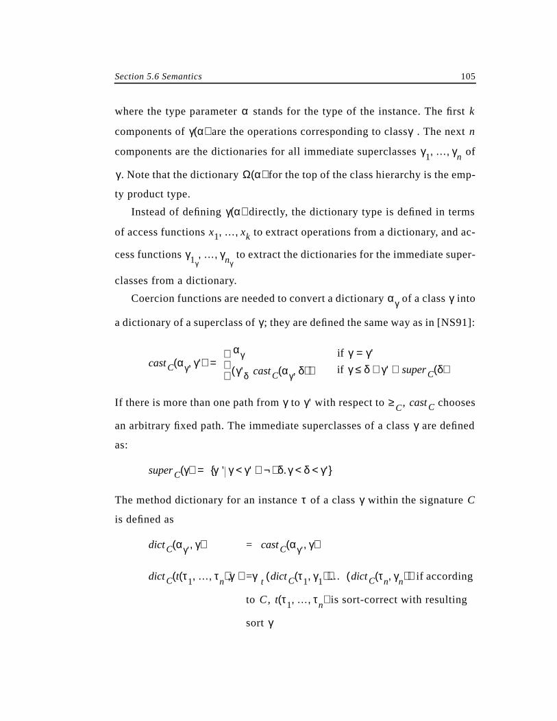
Section 5.6 Semantics 105
where the type parameter stands for the type of the instance. The first
components of are the operations corresponding to class . The next
components are the dictionaries for all immediate superclasses of
. Note that the dictionary for the top of the class hierarchy is the emp-
ty product type.
Instead of defining directly, the dictionary type is defined in terms
of access functions to extract operations from a dictionary, and ac-
cess functions to extract the dictionaries for the immediate super-
classes from a dictionary.
Coercion functions are needed to convert a dictionary of a class into
a dictionary of a superclass of ; they are defined the same way as in [NS91]:
If there is more than one path from to with respect to , chooses
an arbitrary fixed path. The immediate superclasses of a class are defined
as:
The method dictionary for an instance of a class within the signature
is defined as
=
= if according
to , is sort-correct with resulting
sort
α k
γ α( ) γ n
γ1 … γn, ,
γ Ω α( )
γ α( )
x1 … xk, ,
γ1γ… γnγ
, ,
αγ γ
γ
castC αγ γ',( )αγ
γ'δ castC αγ δ,( )( )
if γ γ'=if γ δ≤ γ' superC δ( )∈∧
=
γ γ' ≥ C castC
γ
superC γ( ) γ' γ γ'< δ.∃ γ δ γ'< <¬∧ =
τ γ C
dictC αγ' γ,( ) castC αγ' γ,( )
dictC t τ1 … τn, ,( ) γ,( ) γt dictC τ1 γ1,( )( ) … dictC τn γn,( )( )
C t τ1 … τn, ,( )
γ
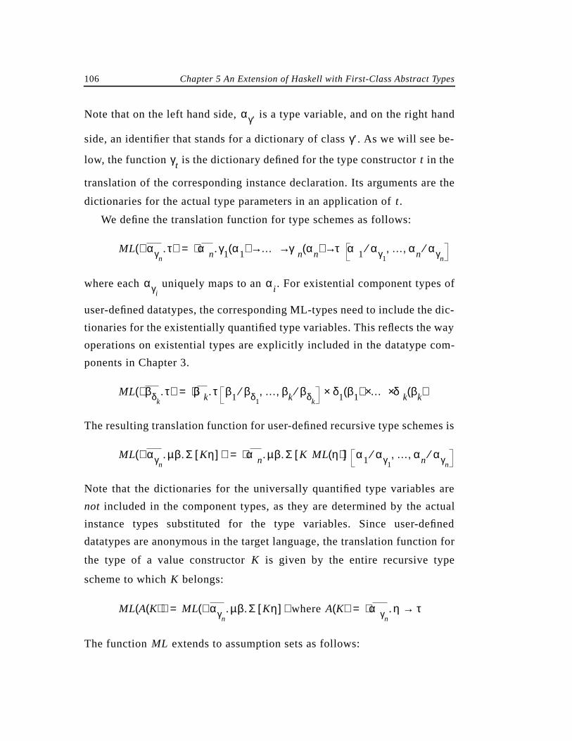
106 Chapter 5 An Extension of Haskell with First-Class Abstract Types
Note that on the left hand side, is a type variable, and on the right hand
side, an identifier that stands for a dictionary of class . As we will see be-
low, the function is the dictionary defined for the type constructor in the
translation of the corresponding instance declaration. Its arguments are the
dictionaries for the actual type parameters in an application of .
We define the translation function for type schemes as follows:
where each uniquely maps to an . For existential component types of
user-defined datatypes, the corresponding ML-types need to include the dic-
tionaries for the existentially quantified type variables. This reflects the way
operations on existential types are explicitly included in the datatype com-
ponents in Chapter 3.
The resulting translation function for user-defined recursive type schemes is
Note that the dictionaries for the universally quantified type variables are
not included in the component types, as they are determined by the actual
instance types substituted for the type variables. Since user-defined
datatypes are anonymous in the target language, the translation function for
the type of a value constructor is given by the entire recursive type
scheme to which belongs:
where
The function extends to assumption sets as follows:
αγ'
γ'
γt t
t
ML αγn.∀ τ( ) αn∀ .γ1 α1( ) … γn αn( ) τ α1 αγ1
⁄ … αn αγn⁄, ,→ → →=
αγiαi
ML βδk∃ .τ( ) βk∃ .τ β1 βδ1
⁄ … βk βδk⁄, , δ1 β1( ) … δk βk( )×××=
ML αγn.∀ µβ.Σ Kη[ ]( ) αn.∀ µβ.Σ K ML η( )[ ] α1 αγ1
⁄ … αn αγn⁄, ,=
K
K
ML A K( )( ) ML αγn.∀ µβ.Σ Kη[ ]( )= A K( ) αγn
.∀ η τ→=
ML
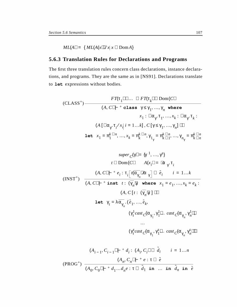
Section 5.6 Semantics 107
5.6.3 Translation Rules for Declarations and Programs
The first three translation rules concern class declarations, instance declara-
tions, and programs. They are the same as in [NS91]. Declarations translate
to expressions without bodies.
(CLASS+)
(INST+)
(PROG+)
ML A( ) ML A x( )( ) x⁄ x DomA∈ =
let
FT τ1( ) … FT τk( )∪ ∪ Dom C( )⊆
A C,( ) |−+ class γ γ1 … γn, ,≤ where
x1 : αγ.∀ τ1 … xk : αγ.∀ τk, , :
A αγ.∀ τi xi⁄ i 1…k=[ ] C γ γ1 … γn, ,≤[ ],( ) ⇒
let x1 π1k n+= … xk πk
k n+= γ1γπk 1+
k n+= … γnγπk n+
k n+=, ,, , ,
superC γ( ) γ1 … γs, , =
t Dom C( )∈ A xi( ) αγ.∀ τi=
A C,( ) |−+ ei : τi t αγn( ) αγ⁄ ei⇒ i 1…k=
A C,( ) |−+ inst t : γn( ) γ where x1 e1= … xk ek=, , :
A C t : γn( ) γ[ ],( ) ⇒
let γt λαγn. ( e1 … ek, , ,=
γt1castC αγ1
γ11,( )…castC αγn
γn1,( )( ) ,
…
γtscastC αγ1
γ1s,( )…castC αγn
γns,( )( ) )
Ai 1− Ci 1−,( ) |−+ di : Ai Ci,( ) di⇒ i 1…n=
An Cn,( ) |−+ e : τ e⇒
A0 C0,( ) |−+ d1…dne : τ d1 in … in dn in e⇒
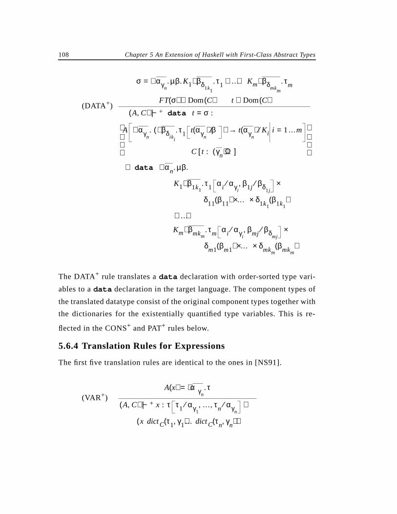
108 Chapter 5 An Extension of Haskell with First-Class Abstract Types
(DATA +)
The DATA+ rule translates adata declaration with order-sorted type vari-
ables to adata declaration in the target language. The component types of
the translated datatype consist of the original component types together with
the dictionaries for the existentially quantified type variables. This is re-
flected in the CONS+ and PAT+ rules below.
5.6.4 Translation Rules for Expressions
The first five translation rules are identical to the ones in [NS91].
(VAR+)
σ αγn.∀ µβ.K1 βδ1k1
.∃ τ1 … Km βδmkm
.∃ τm+ +=
FT σ( ) Dom C( )⊆ t Dom C( )∉A C,( ) |−+ data t σ= :
A αγn.∀ βδiki
.∃ τ1 t αγn( ) β⁄( ) t αγn
( )→ Ki⁄ i 1…m=
C t : γn( ) Ω[ ]
data αn.∀ µβ.⇒
K1 β1k1.∃ τ1 αi αγi
⁄ β1j βδ1j⁄, ×
δ11 β11( ) …× δ1k1β1k1
( )×
…+ +
Km βmkm.∃ τm αi αγi
⁄ βmj βδmj⁄, ×
δm1 βm1( ) …× δmkmβmkm
( )×
A x( ) αγn.∀ τ=
A C,( ) |−+ x : τ τ1 αγ1⁄ … τn αγn
⁄, , ⇒
x dictC τ1 γ1,( )…dictC τn γn,( )( )
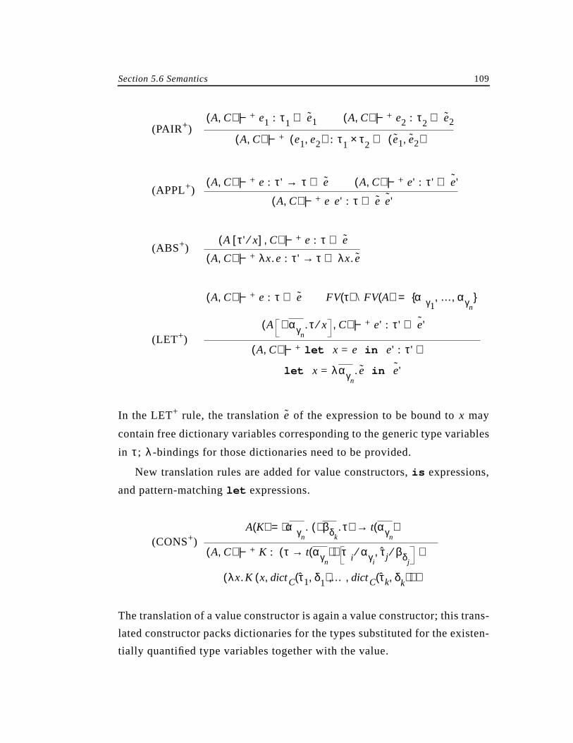
Section 5.6 Semantics 109
(PAIR+)
(APPL+)
(ABS+)
(LET+)
In the LET+ rule, the translation of the expression to be bound to may
contain free dictionary variables corresponding to the generic type variables
in ; -bindings for those dictionaries need to be provided.
New translation rules are added for value constructors,is expressions,
and pattern-matchinglet expressions.
(CONS+)
The translation of a value constructor is again a value constructor; this trans-
lated constructor packs dictionaries for the types substituted for the existen-
tially quantified type variables together with the value.
A C,( ) |−+ e1 : τ1 e1⇒ A C,( ) |−+ e2 : τ2 e2⇒
A C,( ) |−+ e1 e2,( ) : τ1 τ2× e1 e2,( )⇒
A C,( ) |−+ e : τ' → τ e⇒ A C,( ) |−+ e' : τ' e'˜⇒
A C,( ) |−+ e e' : τ e e'˜⇒
A τ' x⁄[ ] C,( ) |−+ e : τ e⇒A C,( ) |−+ λx.e : τ' τ→ λx. e⇒
A C,( ) |−+ e : τ e⇒ FV τ( ) \ FV A( ) αγ1… αγn
, , =
A αγn.∀ τ x⁄ C,( ) |−+ e' : τ' e'˜⇒
A C,( ) |−+ let x = e in e' : τ' ⇒
let x = λαγn. e in e'˜
e x
τ λ
A K( ) αγn.∀ βδk
.∃ τ( ) t αγn( )→=
A C,( ) |−+ K : τ t αγn( )→( ) τi αγi
⁄ τj βδj⁄, ⇒
λx.K x dictC τ1 δ1,( ) … dictC τk δk,( ), ,,( )( )
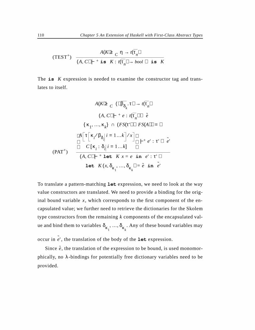
110 Chapter 5 An Extension of Haskell with First-Class Abstract Types
(TEST+)
The expression is needed to examine the constructor tag and trans-
lates to itself.
(PAT+)
To translate a pattern-matchinglet expression, we need to look at the way
value constructors are translated. We need to provide a binding for the orig-
inal bound variable , which corresponds to the first component of the en-
capsulated value; we further need to retrieve the dictionaries for the Skolem
type constructors from the remaining components of the encapsulated val-
ue and bind them to variables . Any of these bound variables may
occur in , the translation of the body of thelet expression.
Since , the translation of the expression to be bound, is used monomor-
phically, no -bindings for potentially free dictionary variables need to be
provided.
A K( ) ≥ C η t τn( )→
A C,( ) |−+ is K : t τn( ) bool→ is K⇒
is K
A K( ) ≥ C βδk.∃ τ( ) t τn( )→
A C,( ) |−+ e : t τn( ) e⇒
κ1 … κk, , FS τ'( ) FS A( )∪( )∩ ∅=
A τ κi βδi⁄ i 1…k= x⁄
C κi : δi i 1…k=[ ]
|−+ e' : τ' e'˜⇒
A C,( ) |−+ let K x = e in e' : τ' ⇒
let K x δκ1… δκk
, , ,( ) = e in e'˜
x
k
δκ1… δκk
, ,
e'˜
e
λ
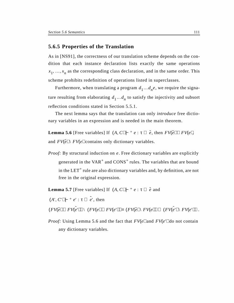
Section 5.6 Semantics 111
5.6.5 Properties of the Translation
As in [NS91], the correctness of our translation scheme depends on the con-
dition that each instance declaration lists exactly the same operations
as the corresponding class declaration, and in the same order. This
scheme prohibits redefinition of operations listed in superclasses.
Furthermore, when translating a program , we require the signa-
ture resulting from elaborating to satisfy the injectivity and subsort
reflection conditions stated in Section 5.5.1.
The next lemma says that the translation can onlyintroduce free dictio-
nary variables in an expression and is needed in the main theorem.
Lemma 5.6 [Free variables] If , then ,
and contains only dictionary variables.
Proof: By structural induction on . Free dictionary variables are explicitly
generated in the VAR+ and CONS+ rules. The variables that are bound
in the LET+ rule are also dictionary variables and, by definition, are not
free in the original expression.
Lemma 5.7 [Free variables] If and
, then
.
Proof: Using Lemma 5.6 and the fact that and do not contain
any dictionary variables.
x1 … xn, ,
d1…dne
d1…dn
A C,( ) |−+ e : τ e⇒ FV e( ) FV e( )⊇
FV e( ) \ FV e( )
e
A C,( ) |−+ e : τ e⇒
A' C',( ) |−+ e' : τ e'˜⇒
FV e( ) FV e'˜( )∪( ) \ FV e( ) FV e'( )∪( ) FV e( ) \ FV e( )( ) FV e'˜( ) \ FV e'( )( )∪=
FV e( ) FV e'( )
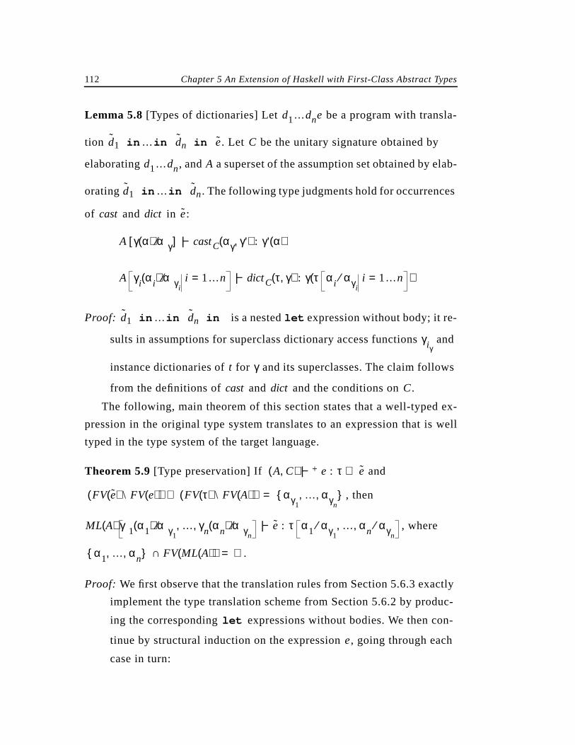
112 Chapter 5 An Extension of Haskell with First-Class Abstract Types
Lemma 5.8 [Types of dictionaries] Let be a program with transla-
tion . Let be the unitary signature obtained by
elaborating , and a superset of the assumption set obtained by elab-
orating . The following type judgments hold for occurrences
of and in :
Proof: is a nestedlet expression without body; it re-
sults in assumptions for superclass dictionary access functions and
instance dictionaries of for and its superclasses. The claim follows
from the definitions of and and the conditions on .
The following, main theorem of this section states that a well-typed ex-
pression in the original type system translates to an expression that is well
typed in the type system of the target language.
Theorem 5.9[Type preservation] If and
, then
, where
.
Proof: We first observe that the translation rules from Section 5.6.3 exactly
implement the type translation scheme from Section 5.6.2 by produc-
ing the corresponding expressions without bodies. We then con-
tinue by structural induction on the expression , going through each
case in turn:
d1…dne
d1 in …in dn in e C
d1…dn A
d1 in …in dn
cast dict e
A γ α( ) αγ⁄[ ] |− castC αγ γ',( ) : γ' α( )
A γi αi( ) αγi⁄ i 1…n= |− dictC τ γ,( ) : γ τ αi αγi
⁄ i 1…n=( )
d1 in …in dn in
γiγ
t γ
cast dict C
A C,( ) |−+ e : τ e⇒
FV e( ) \ FV e( )( ) FV τ( ) \ FV A( )( )∪ αγ1… αγn
, , =
ML A( ) γ1 α1( ) αγ1⁄ … γn αn( ) αγn
⁄, , |− e : τ α1 αγ1⁄ … αn αγn
⁄, ,
α1 … αn, , FV ML A( )( )∩ ∅=
let
e
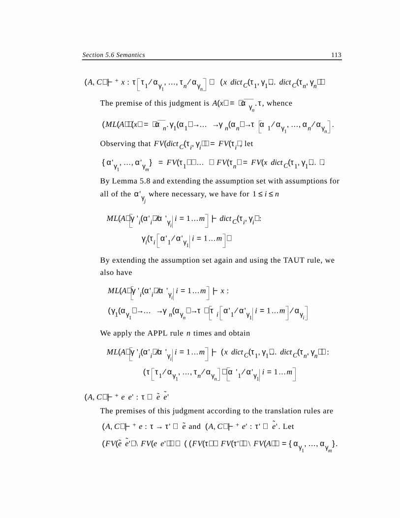
Section 5.6 Semantics 113
The premise of this judgment is , whence
.
Observing that , let
.
By Lemma 5.8 and extending the assumption set with assumptions for
all of the where necessary, we have for
By extending the assumption set again and using the TAUT rule, we
also have
We apply the APPL rule times and obtain
The premises of this judgment according to the translation rules are
and . Let
.
A C,( ) |−+ x : τ τ1 αγ1⁄ … τn αγn
⁄, , x dictC τ1 γ1,( )…dictC τn γn,( )( )⇒
A x( ) αγn.∀ τ=
ML A( )( ) x( ) αn.∀ γ1 α1( ) … γn αn( ) τ α1 αγ1⁄ … αn αγn
⁄, ,→ → →=
FV dictC τi γi,( )( ) FV τi( )=
α'γ1… α'γm
, , FV τ1( ) … FV τn( )∪ ∪ FV x dictC τ1 γ1,( )…( )= =
α'γj1 i n≤ ≤
ML A( ) γ' i α' i( ) α'γi⁄ i 1…m= |− dictC τi γi,( ) :
γi τi α'1 α'γ1⁄ i 1…m=( )
ML A( ) γ' i α' i( ) α'γi⁄ i 1…m= |− x :
γ1 αγ1( ) … γn αγn
( ) τ→ → →( ) τi α'1 α'γ1⁄ i 1…m= αγi
⁄
n
ML A( ) γ' i α' i( ) α'γi⁄ i 1…m= |− x dictC τ1 γ1,( )…dictC τn γn,( )( ) :
τ τ1 αγ1⁄ … τn αγn
⁄, ,( ) α'1 α'γ1⁄ i 1…m=
A C,( ) |−+ e e' : τ e e'˜⇒
A C,( ) |−+ e : τ τ'→ e⇒ A C,( ) |−+ e' : τ' e'˜⇒
FV e e'˜( ) \ FV e e'( )( ) FV τ( ) FV τ'( )∪( ) \ FV A( )( )∪ αγ1… αγm
, , =
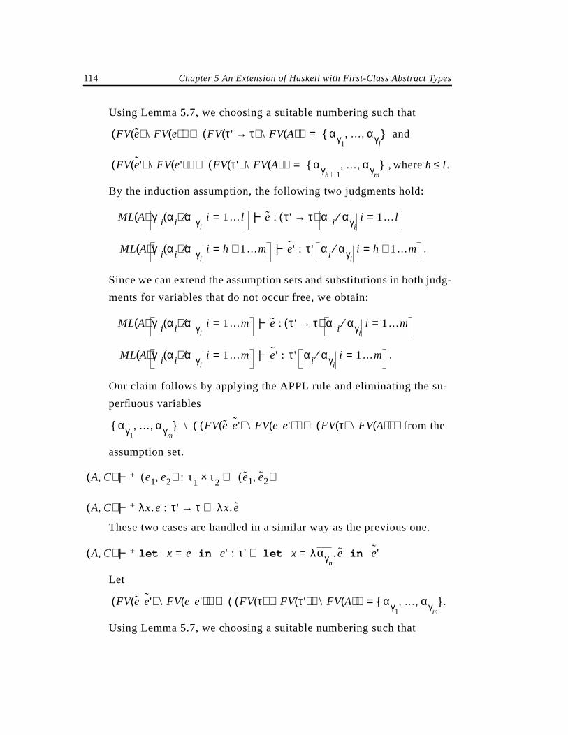
114 Chapter 5 An Extension of Haskell with First-Class Abstract Types
Using Lemma 5.7, we choosing a suitable numbering such that
and
, where .
By the induction assumption, the following two judgments hold:
.
Since we can extend the assumption sets and substitutions in both judg-
ments for variables that do not occur free, we obtain:
.
Our claim follows by applying the APPL rule and eliminating the su-
perfluous variables
from the
assumption set.
These two cases are handled in a similar way as the previous one.
Let
.
Using Lemma 5.7, we choosing a suitable numbering such that
FV e( ) \ FV e( )( ) FV τ' τ→( ) \ FV A( )( )∪ αγ1… αγl
, , =
FV e'˜( ) \ FV e'( )( ) FV τ'( ) \ FV A( )( )∪ αγh 1+… αγm
, , = h l≤
ML A( ) γi αi( ) αγi⁄ i 1…l= |− e : τ' τ→( ) αi αγi
⁄ i 1…l=
ML A( ) γi αi( ) αγi⁄ i h 1…m+= |− e'˜ : τ' αi αγi
⁄ i h 1…m+=
ML A( ) γi αi( ) αγi⁄ i 1…m= |− e : τ' τ→( ) αi αγi
⁄ i 1…m=
ML A( ) γi αi( ) αγi⁄ i 1…m= |− e'˜ : τ' αi αγi
⁄ i 1…m=
αγ1… αγm
, , \ FV e e'˜( ) \ FV e e'( )( ) FV τ( ) \ FV A( )( )∪( )
A C,( ) |−+ e1 e2,( ) : τ1 τ2× e1 e2,( )⇒
A C,( ) |−+ λx.e : τ' τ→ λx. e⇒
A C,( ) |−+ let x = e in e' : τ' let x = λαγn. e in e'˜⇒
FV e e'˜( ) \ FV e e'( )( ) FV τ( ) FV τ'( )∪( ) \ FV A( )( )∪ αγ1… αγm
, , =
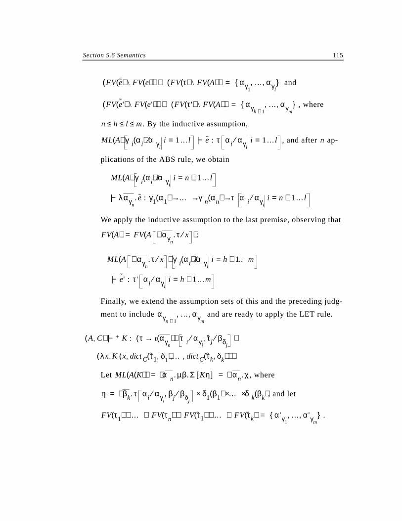
Section 5.6 Semantics 115
and
, where
. By the inductive assumption,
, and after ap-
plications of the ABS rule, we obtain
We apply the inductive assumption to the last premise, observing that
:
Finally, we extend the assumption sets of this and the preceding judg-
ment to include and are ready to apply the LET rule.
Let , where
, and let
.
FV e( ) \ FV e( )( ) FV τ( ) \ FV A( )( )∪ αγ1… αγl
, , =
FV e'˜( ) \ FV e'( )( ) FV τ'( ) \ FV A( )( )∪ αγh 1+… αγm
, , =
n h l m≤ ≤ ≤
ML A( ) γi αi( ) αγi⁄ i 1…l= |− e : τ αi αγi
⁄ i 1…l= n
ML A( ) γi αi( ) αγi⁄ i n 1…l+=
|− λαγn. e : γ1 α1( ) … γn αn( ) τ αi αγi
⁄ i n 1…l+=→ → →
FV A( ) FV A αγn.∀ τ x⁄( )=
ML A αγn.∀ τ x⁄( ) γi αi( ) αγi
⁄ i h 1+ …m=
|− e'˜ : τ' αi αγi⁄ i h 1…m+=
αγn 1+… αγm
, ,
A C,( ) |−+ K : τ t αγn( )→( ) τi αγi
⁄ τj βδj⁄, ⇒
λx.K x dictC τ1 δ1,( ) … dictC τk δk,( ), ,,( )( )
ML A K( )( ) αn.∀ µβ.Σ Kη[ ] αn.∀ χ= =
η βk∃ .τ αi αγi⁄ βj βδj
⁄, δ1 β1( ) … δk βk( )×××=
FV τ1( ) … FV τn( ) FV∪ ∪ ∪ τ1( ) … FV τk( )∪ ∪ α'γ1… α'γm
, , =
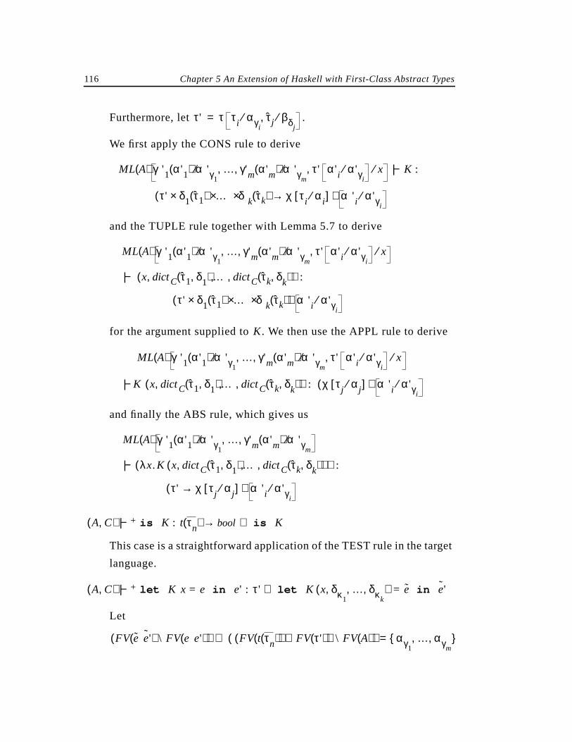
116 Chapter 5 An Extension of Haskell with First-Class Abstract Types
Furthermore, let .
We first apply the CONS rule to derive
and the TUPLE rule together with Lemma 5.7 to derive
for the argument supplied to . We then use the APPL rule to derive
and finally the ABS rule, which gives us
This case is a straightforward application of the TEST rule in the target
language.
Let
τ' τ τi αγi⁄ τj βδj
⁄,=
ML A( ) γ'1 α'1( ) α'γ1⁄ … γ'm α'm( ) α'γm
⁄ τ' α' i α'γi⁄ x⁄, , , |− K :
τ' δ1 τ1( ) … δk τk( )××× χ τi αi⁄[ ]→( ) α' i α'γi⁄
ML A( ) γ'1 α'1( ) α'γ1⁄ … γ'm α'm( ) α'γm
⁄ τ' α' i α'γi⁄ x⁄, , ,
|− x dictC τ1 δ1,( ) … dictC τk δk,( ), ,,( ) :
τ' δ× 1 τ1( ) … δk τk( )××( ) α' i α'γi⁄
K
ML A( ) γ'1 α'1( ) α'γ1⁄ … γ'm α'm( ) α'γm
⁄ τ' α' i α'γi⁄ x⁄, , ,
|− K x dictC τ1 δ1,( ) … dictC τk δk,( ), ,,( ) : χ τj αj⁄[ ]( ) α' i α'γi⁄
ML A( ) γ'1 α'1( ) α'γ1⁄ … γ'm α'm( ) α'γm
⁄, ,
|− λx.K x dictC τ1 δ1,( ) … dictC τk δk,( ), ,,( )( ) :
τ' χ τj αj⁄[ ]→( ) α' i α'γi⁄
A C,( ) |−+ is K : t τn( ) bool→ is K⇒
A C,( ) |−+ let K x = e in e' : τ' let K x δκ1… δκk
, , ,( ) = e in e'˜⇒
FV e e'˜( ) \ FV e e'( )( ) FV t τn( )( ) FV τ'( )∪( ) \ FV A( )( )∪ αγ1… αγm
, , =
Section 5.6 Semantics 117
choosing a suitable numbering such that
and
, where
.
Let , where
.
By the induction assumption,
, where
. We further apply the in-
duction assumption to the last premise to obtain
Note that in . We now extend the assumption sets
of this and the preceding judgment to include , and apply
the PAT’’ rule. Our claim follows after restricting the final assumption
set to .
The following corollary is a deterministic version of the type preserva-
tion theorem in [NS91]. It covers the case of unambiguous resulting expres-
sions, that is, expressions whose translations do not contain free dictionary
variables not free in their types.
FV e( ) \ FV e( )( ) FV t τn( )( ) \ FV A( )( )∪ αγ1… αγl
, , =
FV e'˜( ) \ FV e'( )( ) FV τ'( ) \ FV A( )( )∪ αγh 1+… αγm
, , =
h l m≤ ≤
α'n.∀ µβ.Σ K βk.∃ τ[ ] ML σ( )=
τ τ β1 βδ1⁄ … βk βδk
⁄, , δ1 β1( ) … δk βk( )×××=
ML A( ) γi αi( ) αγi⁄ i 1…l= |− e : t αi αγi
⁄ i 1…l=
t µβ.Σ K βk.∃ τ[ ]( ) τ1 α'γ1⁄ … τn α'γn
⁄, ,=
ML A( )γi αi( ) αγi
⁄ i h 1…m+=
τ κj βδj⁄ x⁄ δ1 κ1( ) δκ1
⁄ … δk κk( ) δκk⁄, , ,
|− e'˜ : τ' αi αγi⁄ i h 1…m+=
dictC' κj δj,( ) δκj= e'˜
αγ1… αγm
, ,
FV e e'˜( ) \ FV e e'( )( ) FV τ'( ) \ FV A( )( )∪
118 Chapter 5 An Extension of Haskell with First-Class Abstract Types
Corollary 5.10 [Type preservation] Let all types in the range of be closed.
If and , then
, where
.
Proof: We use the preceding theorem and apply the ABS rule from
Chapter 3 successive times.
Corollary 5.11 [Semantic soundness] Let all types in the range of be
closed, and let be a type environment such that for every ,
. If and , then
.
Proof: By type preservation and semantic soundness of the target language.
A
A C,( ) |−+ e : τ e⇒ FV e( ) \ FV e( ) FV τ( )⊆
ML A( ) |− λαγn. e : γ1 α1( ) … γn αn( ) τ α1 αγ1
⁄ … αn αγn⁄, ,→ → →
α1 … αn, , FV ML A( )( )∩ ∅=
n
A
ψ α Domψ∈
wrong ψ α( )∉ A C,( ) |−+ e : τ e⇒ |= ρ ψ, ML A( )
E [[ e]] ρ wrong≠
119
6 Related Work, Future Work, andConclusions
6.1 Related Work
The following table compares our work with other programming languages
with similar features or objectives. The design criteria used as a basis for
our comparison are taken from Section 1.1:
1. Strong and static typing,
2. type reconstruction,
3. higher-order functions,
4. parametric polymorphism,
5. extensible abstract types with multiple implementations, and
6. first-class abstract types.
In the table, means the feature is supported, means it is not fully sup-
ported, and a blank entry means it is not supported at all.
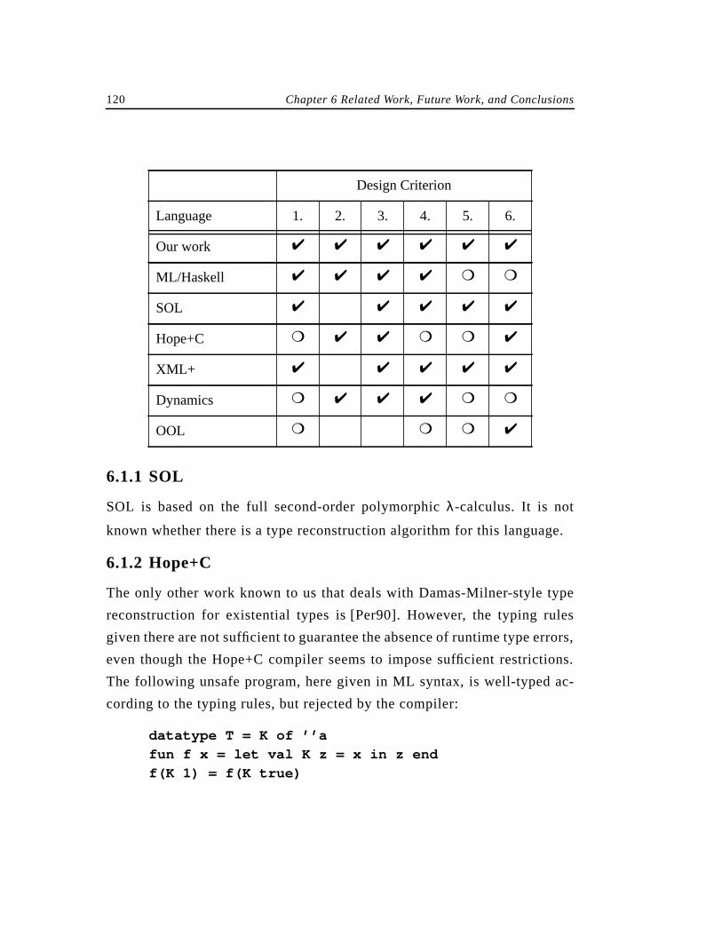
120 Chapter 6 Related Work, Future Work, and Conclusions
6.1.1 SOL
SOL is based on the full second-order polymorphicλ-calculus. It is not
known whether there is a type reconstruction algorithm for this language.
6.1.2 Hope+C
The only other work known to us that deals with Damas-Milner-style type
reconstruction for existential types is [Per90]. However, the typing rules
given there are not sufficient to guarantee the absence of runtime type errors,
even though the Hope+C compiler seems to impose sufficient restrictions.
The following unsafe program, here given in ML syntax, is well-typed ac-
cording to the typing rules, but rejected by the compiler:
datatype T = K of ’’a
fun f x = let val K z = x in z end
f(K 1) = f(K true)
Design Criterion
Language 1. 2. 3. 4. 5. 6.
Our work
ML/Haskell
SOL
Hope+C
XML+
Dynamics
OOL
Section 6.1 Related Work 121
In addition, an identifier bound in a pattern-matchinglet expression is not
polymorphic according to the typing rules. This restriction does not apply to
our work.
6.1.3 XML+
The possibility of making ML structures first-class by implicitly hiding their
type components is discussed in [MMM91] without addressing the issue of
type inference. By hiding the type components of a structure, its type is im-
plicitly coerced from a strong sum type to an existential type. Detailed dis-
cussions of sum types can be found in [Mac86] [MH88].
6.1.4 Dynamics in ML
An extension of ML with objects that carry dynamic type information is de-
scribed in [LM91]. A dynamic is a pair consisting of a value and the type of
the value. Such an object is constructed from a value by applying the con-
structordynamic . The object can then be dynamically coerced by pattern
matching on both the value and the runtime type. Existential types are used
to match dynamic values against dynamic patterns with incomplete type in-
formation. Dynamics are useful for typing functions such aseval . Howev-
er, they do not provide type abstraction, since they give access to the type
of an object at runtime. It seems possible to combine their system with ours,
extending their existential patterns to existential types. We are currently in-
vestigating this point.
6.1.5 Object-Oriented Languages
Most statically typed object-oriented languages identify subclassing with
subtyping (C++ [Str86], Modula-3 [CDG+89]) at the expense of severely re-
stricting the expressive power of the language. Due to thecontravariance
rule for function subtyping, not even simple algebraic structures can be de-
scribed in C++; this is discussed in detail in [CHC90] [HL91].
122 Chapter 6 Related Work, Future Work, and Conclusions
Recognizing and attempting to overcome this restriction, other languag-
es sacrifice static typing (Eiffel [Mey92], Ada 9X [dod91]) and rely on run
time checks to guarantee compatibility of function arguments.
Furthermore, most object-oriented languages do not support type recon-
struction; a recent advance in type reconstruction for a Smalltalk-like lan-
guage is presented in [PS91].
6.2 Current State of Implementation
We have implemented a Standard ML prototype of an interpreter with type
reconstruction for our core language, Mini-ML [CDDK86] extended with
recursive datatypes over existentially quantified component types. The ML-
style examples from this thesis have been developed and tested using our in-
terpreter.
Technically, the interpreter consists of the following components:
• Lexer and parser were built using the tools ML-Lex [AMT89] and ML-
Yacc [TA91], respectively.
• The type reconstruction phase is based on [Han87].
• The evaluator directly implements the denotational semantics present-
ed in Section 3.6.2.
We plan further to develop this prototype towards an interpreter of a full lan-
guage based on our extension of SML.
The latest releases of the Lazy ML [AJ92] and Haskell B. [Aug92] sys-
tems feature datatypes with existentially quantified component types. Both
systems were developed at the Chalmers University of Technology; they
provide full compilers and interpreters capable of dealing with larger pro-
grams. The Haskell examples from this thesis have been tested using the
Chalmers Haskell B. interpreter.
6.3 Conclusions
The question we had set out to answer in this dissertation was:
Section 6.4 Future Work 123
Is it feasible to design a high-level programming language that satis-
fies criteria1. through6.?
We showed that such a design is feasible from a type-theoretic, a language
design, and an implementation perspective:
• Type-theoretic view: Static typing and semantic soundness of the type
systems hold for all three languages presented. Furthermore, we ex-
tended the Damas-Milner type reconstruction algorithm used in ML to
cope with our languages.
• Language design view: Our examples demonstrated that we gain con-
siderable expressiveness and flexibility by adding first-class abstract
types to ML and Haskell while retaining the syntactic and semantic
“look and feel” of the original languages.
• Implementation view: Our prototype implementation shows that our
languages can be implemented using standard techniques as the ones
described in [Han87] or used in the Standard ML of New Jersey imple-
mentation [AM92]. The Chalmers LML and HBC systems demonstrate
that it is feasible to implement our extensions in practical compilers
and interpreters.
6.4 Future Work
Our work leads off to a number of future research directions, some of which
are discussed below.
6.4.1 Combination of Modules and Existential Quantification
in ML
We demonstrated in Chapter 5 how Haskell type classes can be used as sig-
natures of abstract data types. The ML module system also provides signa-
tures, which are strong sum types. One could imagine using these signatures
to describe interfaces of abstract types. First-class abstract types could then
124 Chapter 6 Related Work, Future Work, and Conclusions
be achieved by applying an injection that makes the type components of the
signature existentially quantified, along the lines of [MMM91].
6.4.2 A Polymorphic Pattern-Matching let Expression
An identifier bound using the pattern-matching expression from
Chapter 5 is monomorphic, whereas an identifier bound by the correspond-
ing expression from Chapter 3 can be used polymorphically. It would be de-
sirable to overcome this restriction by exploring an extended target lan-
guage, where a function depending on some method dictionaries can be de-
composed before being applied to any arguments. While unsound in the
general case, we conjecture that this is sound in our case, since the argu-
ments are the same whenever the bound identifier is used with the same type.
6.4.3 Combination of Parameterized Type Classes and
Existential Types in Haskell
Type classes in Haskell are not parameterized, thus we cannot model ab-
stract container classes. This shortcoming was discussed in [LO91] and is
also present in our extension of Haskell described in Chapter 5; thus the
stack example from Section 5.2.2 is not polymorphic. An extension of
Haskell with parameterized type classes was recently presented in [CHO92];
it would be desirable to apply the same extension to our language. We con-
jecture that parameterized type classes are an orthogonal extension and
combine well with existential quantification.
Another interesting extension of Haskell is one with a dotless dot nota-
tion analogous to the ML extension from Chapter 4; it appears that such a
language could be translated into the language described in Chapter 5.
6.4.4 Existential Types and Mutable State
Since the full ML language also provides polymorphic references, an exten-
sion of this language with existential types would depend on the coexistence
of existential types and polymorphic references. Similar considerations hold
for other forms of mutable state such as linear types [Ode91] [Wad90].
let
Section 6.4 Future Work 125
6.4.5 Full Implementation
Whereas implementations of Lazy ML and Haskell B. extended with exis-
tential types are now available, further implementation work could be envi-
sioned both at the ML level and at the Haskell level.
At the ML level, the language would be strict and include datatypes with
existentially quantified component types, polymorphic references, and pos-
sibly modules.
At the Haskell level, the language could be strict or non-strict and in-
clude existential quantification over parameterized type classes. Alternative
implementation strategies for Haskell or similar languages with type classes
could be explored; instead of translating to an ML-like language, type class-
es could be mapped to C++ templates [Ode92]. A possible starting point for
further exploration could be an explicitly typed version of Mini-Haskell in
the spirit of [MH88].
126 Chapter 6 Related Work, Future Work, and Conclusions
127
Bibliography
[Aba92] M. Abadi. Private communication, June 1992.
[AJ92] L. Augustsson and T. Johnsson. Lazy ML user manual. July
1992.
[AM92] A. Appel and D. MacQueen. Standard ML of New Jersey. In
Proc. 19th ACM Symp. on Principles of Programming
Languages (POPL), January 1992.
[AMT89] A. Appel, J. Mattson, and D. Tarditi. A lexical analyzer
generator for Standard Ml. Part of the Standard ML of NJ
Distribution, December 1989.
[Aug92] L. Augustsson. Haskell B. user manual. July 1992.
[Bar84] H. Barendregt. The Lambda Calculus: Its Syntax and
Semantics, volume 103 ofStudies in Logic and the Foundations
of Mathematics. North-Holland, 1984.
[BM92] K. Bruce and J. Mitchell. PER models of subtyping, recursive
types and higher-order polymorphism. InProc. 19th ACM
Symp. on Principles of Programming Languages (POPL), pages
316–327, January 1992.
128 Bibliography
[CDDK86] D. Clement, J. Despeyroux, T. Despeyroux, and G. Kahn. A
simple applicative language: Mini-ML. InProc. ACM Conf.
Lisp and Functional Programming, pages 13–27, 1986.
[CDG+89] L. Cardelli, J. Donahue, L. Glassman, M. Jordan, B. Kalsow,
and G. Nelson.Modula-3 Report (revised), Oct. 1989.
[CHC90] W. Cook, W. Hill, and P. Canning. Inheritance is not subtyping.
In Proc. ACM Symp. on Principles of Programming Languages,
pages 125–135, Jan. 1990.
[CHO92] K. Chen, P. Hudak, and M. Odersky. Parametric type classes. In
Proc. ACM Conf. Lisp and Functional Programming, 1992.
[CL90] L. Cardelli and X. Leroy. Abstract types and the dot notation.
In Proc. IFIP Working Conference on Programming Concepts
and Methods, pages 466–491, Sea of Gallilee, Israel, April
1990.
[CW85] L. Cardelli and P. Wegner. On understanding types, data
abstraction and polymorphism.ACM Computing Surveys,
17(4):471–522, Dec. 1985.
[Dam85] L. Damas.Type Assignment in Programming Languages. PhD
thesis, University of Edinburgh, 1985.
[DM82] L. Damas and R. Milner. Principal type schemes for functional
programs. InProc. 9th Annual ACM Symp. on Principles of
Programming Languages, pages 207–212, Jan. 1982.
[dod91] Ada 9x mapping rationale, 1991. United States Department of
Defense.
[FGJM85] K. Futatsugi, J. Goguen, J.-P. Jouannaud, and J. Meseguer.
Principles of OBJ2. InProc. 12th ACM Symp. on Principles of
Programming Languages (POPL), pages 52–66, January 1985.
Bibliography 129
[Han87] P. Hancock. Polymorphic type checking. In S. Peyton-Jones,
editor, The Implementation of Functional Programming
Languages, chapter 8. Prentice-Hall, 1987.
[Har90] R. Harper. Introduction to Standard ML. Technical report,
Carnegie Mellon University, September 1990.
[HL91] F. Henglein and K. Läufer. Programming with structures,
functions, and objects. InProc. XVII Latin American
Informatics Conference (PANEL ’91), pages 333–352. USB,
1991.
[HPJW+92] P. Hudak, S. Peyton-Jones, P. Wadler, et al. Report on the
programming language Haskell A non-strict, purely functional
language Version 1.2.ACM SIGPLAN Notices, 27(5), May
1992.
[LM91] X. Leroy and M. Mauny. Dynamics in ML. InProc. Functional
Programming Languages and Computer Architecture, pages
406–426. ACM, 1991.
[LO91] K. Läufer and M. Odersky. Type classes are signatures of
abstract types. InProc. Phoenix Seminar and Workshop on
Declarative Programming, November 1991.
[Mac86] D. MacQueen. Using dependent types to express modular
structure. In Proc. 13th ACM Symp. on Principles of
Programming Languages, pages 277–286. ACM, Jan. 1986.
[Mey92] B. Meyer.Eiffel The Language. Prentice-Hall, 1992.
[MGS89] J. Meseguer, J. Goguen, and G. Smolka. Order-sorted
unification.J. Symbolic Computation, (8):383–413, 1989.
[MH88] J. Mitchell and R. Harper. The essence of ML. InProc. Symp.
on Principles of Programming Languages. ACM, Jan. 1988.
130 Bibliography
[Mil78] R. Milner. A theory of type polymorphism in programming.J.
Computer and System Sciences, 17:348–375, 1978.
[MM82] A. Martelli and U. Montanari. An efficient unification
algorithm.ACM Transactions on Programming Languages and
Systems, 4(2):258–282, Apr. 1982.
[MMM91] J. Mitchell, S. Meldal, and N. Madhav. An extension of
Standard ML modules with subtyping and inheritance. InProc.
ACM Symp. on Principles of Programming Languages, Jan.
1991.
[MP88] J. Mitchell and G. Plotkin. Abstract types have existential type.
ACM Trans. on Programming Languages and Systems,
10(3):470–502, 1988.
[MPS86] D. MacQueen, G. Plotkin, and R. Sethi. An ideal model for
recursive polymorphic types.Information and Control, 71,
1986.
[MTH90] R. Milner, M. Tofte, and R. Harper.The Definition of Standard
ML. MIT Press, 1990.
[NS91] T. Nipkow and G. Snelting. Type classes and overloading
resolution via order-sorted unification. InProc. Functional
Programming Languages and Computer Architecture, pages 1–
14. ACM, 1991.
[Ode91] M. Odersky. Objects and subtyping in a functional perspective.
IBM Research Report RC 16423, 1991.
[Ode91b] M. Odersky. How to make destructive updates less destructive.
In Proc. 18th ACM Symp. on Principles of Programming
Languages (POPL), January 1991.
Bibliography 131
[Ode92] M. Odersky. Translating type classes to C++ templates. Private
communication, March 1992.
[Per90] N. Perry. The Implementation of Practical Functional
Programming Languages. PhD thesis, Imperial College, 1990.
[PJ87] S. Peyton-Jones. The Implementation of Functional
Programming Languages. Prentice-Hall, 1987.
[Plo83] G. Plotkin. Domains. Course notes, 1983. TeX-ed edition.
[PS91] J. Palsberg and M. Schwartzbach. Object-oriented type
inference. InProc. ACM Conf. Object-Oriented Programming:
Systems, Languages, Applications (OOPSLA), pages 146–165,
1991.
[Rob65] J. Robinson. A machine-oriented logic based on the resolution
principle.J. Assoc. Comput. Mach., 12(1):23–41, 1965.
[Smy77] M. Smyth. Effectively given domains.Theoretical Computer
Science, 5:257–274, 1977.
[SS71] D. Scott and Ch. Strachey. Toward a mathematical semantics
for computer languages. InProc. Symp. on Computers and
Automata, pages 19–46, Brooklyn, New York, 1971. MRI
Symp. Proc‘s, Vol. XXI.
[SS85] M. Schmidt-Schauss. A many-sorted calculus with
polymorphic functions based on resulution and
paramodulation. In Proc. 9th Int. Joint Conf. Artificial
Intelligence, pages 1162–1168, 1985.
[Str86] B. Stroustrup.The C++ Programming Language. Addison-
Wesley, 1986.
[TA91] D. Tarditi and A. Appel. ML-Yacc Version 2.1. Part of the
Standard ML of NJ Distribution, March 1991.
132 Bibliography
[Wad90] P. Wadler. Linear types can change the world. InIFIP TC2
Working Conference on Programming Concepts and Methods,
April 1990.
[WB89] P. Wadler and S. Blott. How to make ad-hoc polymorphism less
ad hoc. InProc. 16th Annual ACM Symp. on Principles of
Programming Languages, pages 60–76. ACM, Jan. 1989.