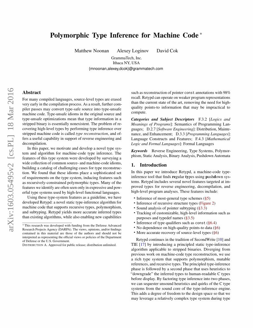
Polymorphic Type Inference for Machine Code ∗

Matthew Noonan Alexey Loginov David CokGrammaTech, Inc.Ithaca NY, USA

{mnoonan,alexey,dcok}@grammatech.com

AbstractFor many compiled languages, source-level types are erasedvery early in the compilation process. As a result, further com-piler passes may convert type-safe source into type-unsafemachine code. Type-unsafe idioms in the original source andtype-unsafe optimizations mean that type information in astripped binary is essentially nonexistent. The problem of re-covering high-level types by performing type inference overstripped machine code is called type reconstruction, and of-fers a useful capability in support of reverse engineering anddecompilation.

In this paper, we motivate and develop a novel type sys-tem and algorithm for machine-code type inference. Thefeatures of this type system were developed by surveying awide collection of common source- and machine-code idioms,building a catalog of challenging cases for type reconstruc-tion. We found that these idioms place a sophisticated setof requirements on the type system, inducing features suchas recursively-constrained polymorphic types. Many of thefeatures we identify are often seen only in expressive and pow-erful type systems used by high-level functional languages.

Using these type-system features as a guideline, we havedeveloped Retypd: a novel static type-inference algorithm formachine code that supports recursive types, polymorphism,and subtyping. Retypd yields more accurate inferred typesthan existing algorithms, while also enabling new capabilities

∗ This research was developed with funding from the Defense AdvancedResearch Projects Agency (DARPA). The views, opinions, and/or findingscontained in this material are those of the authors and should not beinterpreted as representing the official views or policies of the Departmentof Defense or the U.S. Government.DISTRIBUTION A. Approved for public release; distribution unlimited.

such as reconstruction of pointer const annotations with 98%recall. Retypd can operate on weaker program representationsthan the current state of the art, removing the need for high-quality points-to information that may be impractical tocompute.

Categories and Subject Descriptors F.3.2 [Logics andMeanings of Programs]: Semantics of Programming Lan-guages; D.2.7 [Software Engineering]: Distribution, Mainte-nance, and Enhancement; D.3.3 [Programming Languages]:Language Constructs and Features; F.4.3 [MathematicalLogic and Formal Languages]: Formal Languages

Keywords Reverse Engineering, Type Systems, Polymor-phism, Static Analysis, Binary Analysis, Pushdown Automata

1. IntroductionIn this paper we introduce Retypd, a machine-code type-inference tool that finds regular types using pushdown sys-tems. Retypd includes several novel features targeted at im-proved types for reverse engineering, decompilation, andhigh-level program analyses. These features include:

• Inference of most-general type schemes (§5)• Inference of recursive structure types (Figure 2)• Sound analysis of pointer subtyping (§3.3)• Tracking of customizable, high-level information such as

purposes and typedef names (§3.5)• Inference of type qualifiers such as const (§6.4)• No dependence on high-quality points-to data (§6)• More accurate recovery of source-level types (§6)

Retypd continues in the tradition of SecondWrite [10] andTIE [17] by introducing a principled static type-inferencealgorithm applicable to stripped binaries. Diverging fromprevious work on machine-code type reconstruction, we usea rich type system that supports polymorphism, mutablereferences, and recursive types. The principled type-inferencephase is followed by a second phase that uses heuristics to“downgrade” the inferred types to human-readable C typesbefore display. By factoring type inference into two phases,we can sequester unsound heuristics and quirks of the C typesystems from the sound core of the type-inference engine.This adds a degree of freedom to the design space so that wemay leverage a relatively complex type system during type

arX

iv:1

603.

0549

5v2

[cs

.PL

] 1

8 M

ar 2

016

analysis, yet still emit familiar C types for the benefit of thereverse engineer.

Retypd operates on an intermediate representation (IR)recovered by automatically disassembling a binary usingGrammaTech’s static analysis tool CodeSurfer® for Binaries[5]. By generating type constraints from a TSL-based abstractinterpreter [18], Retypd can operate uniformly on binariesfor any platform supported by CodeSurfer, including x86,x86-64, and ARM.

During the development of Retypd, we carried out an ex-tensive investigation of common machine-code idioms incompiled C and C++ code that create challenges for existingtype-inference methods. For each challenging case, we iden-tified requirements for any type system that could correctlytype the idiomatic code. The results of this investigation ap-pear in §2. The type system used by Retypd was specificallydesigned to satisfy these requirements. These common id-ioms pushed us into a far richer type system than we had firstexpected, including features like recursively constrained typeschemes that have not previously been applied to machine-code type inference.

Due to space limitations, details of the proofs and algo-rithms appear in the appendices, which are available in the on-line version of this paper at arXiv:1603.05495 [22]. Scriptsand data sets used for evaluation also appear there.

2. ChallengesThere are many challenges to carrying out type inferenceon machine code, and many common idioms that lead tosophisticated demands on the feature set of a type system.In this section, we describe several of the challenges seenduring the development of Retypd that led to our particularcombination of type-system features.

2.1 Optimizations after Type ErasureSince type erasure typically happens early in the compilationprocess, many compiler optimizations may take well-typedmachine code and produce functionally equivalent but ill-typed results. We found that there were three common op-timization techniques that required special care: the use ofa variable as a syntactic constant, early returns along errorpaths, and the re-use of stack slots.

Semi-syntactic constants: Suppose a function with signaturevoid f(int x, char* y) is invoked as f(0, NULL). Thiswill usually be compiled to x86 machine code similar to

xor eax , eaxpush eax ; y := NULLpush eax ; x := 0call f

This represents a code-size optimization, since push eax canbe encoded in one byte instead of the five bytes needed topush an immediate value (0). We must be careful that thetype variables for x and y are not unified; here, eax is being

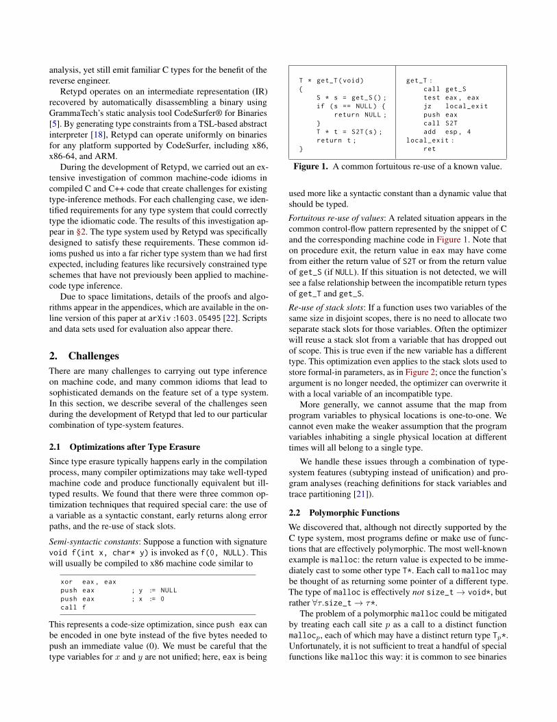
T * get_T(void){

S * s = get_S ();if (s == NULL) {

return NULL;}T * t = S2T(s);return t;

}

get_T:call get_Stest eax , eaxjz local_exitpush eaxcall S2Tadd esp , 4

local_exit:ret

Figure 1. A common fortuitous re-use of a known value.

used more like a syntactic constant than a dynamic value thatshould be typed.

Fortuitous re-use of values: A related situation appears in thecommon control-flow pattern represented by the snippet of Cand the corresponding machine code in Figure 1. Note thaton procedure exit, the return value in eax may have comefrom either the return value of S2T or from the return valueof get_S (if NULL). If this situation is not detected, we willsee a false relationship between the incompatible return typesof get_T and get_S.

Re-use of stack slots: If a function uses two variables of thesame size in disjoint scopes, there is no need to allocate twoseparate stack slots for those variables. Often the optimizerwill reuse a stack slot from a variable that has dropped outof scope. This is true even if the new variable has a differenttype. This optimization even applies to the stack slots used tostore formal-in parameters, as in Figure 2; once the function’sargument is no longer needed, the optimizer can overwrite itwith a local variable of an incompatible type.

More generally, we cannot assume that the map fromprogram variables to physical locations is one-to-one. Wecannot even make the weaker assumption that the programvariables inhabiting a single physical location at differenttimes will all belong to a single type.

We handle these issues through a combination of type-system features (subtyping instead of unification) and pro-gram analyses (reaching definitions for stack variables andtrace partitioning [21]).

2.2 Polymorphic FunctionsWe discovered that, although not directly supported by theC type system, most programs define or make use of func-tions that are effectively polymorphic. The most well-knownexample is malloc: the return value is expected to be imme-diately cast to some other type T*. Each call to malloc maybe thought of as returning some pointer of a different type.The type of malloc is effectively not size_t→ void*, butrather ∀τ.size_t→ τ*.

The problem of a polymorphic malloc could be mitigatedby treating each call site p as a call to a distinct functionmallocp, each of which may have a distinct return type Tp*.Unfortunately, it is not sufficient to treat a handful of specialfunctions like malloc this way: it is common to see binaries

#include <stdlib.h>

struct LL{

struct LL * next;int handle;

};

int close_last(struct LL * list){

while (list ->next != NULL){

list = list ->next;}return close(list ->handle );

}

close_last:push ebpmov ebp ,espsub esp ,8mov edx ,dword [ebp+arg_0]jmp loc_8048402

loc_8048400:mov edx ,eax

loc_8048402:mov eax ,dword [edx]test eax ,eaxjnz loc_8048400mov eax ,dword [edx+4]mov dword [ebp+arg_0],eaxleavejmp __thunk_.close

∀F. (∃τ.C)⇒F where C =

F.instack0 v ττ.load.σ32@0 v ττ.load.σ32@4 v int ∧#FileDescriptor

int ∨#SuccessZ v F.outeax

typedef struct {Struct_0 * field_0;int // #FileDescriptor

field_4;} Struct_0;

int // #SuccessZclose_last(const Struct_0 *);

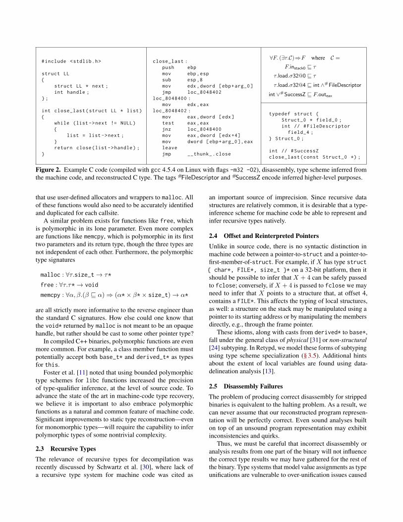
Figure 2. Example C code (compiled with gcc 4.5.4 on Linux with flags -m32 -O2), disassembly, type scheme inferred fromthe machine code, and reconstructed C type. The tags #FileDescriptor and #SuccessZ encode inferred higher-level purposes.

that use user-defined allocators and wrappers to malloc. Allof these functions would also need to be accurately identifiedand duplicated for each callsite.

A similar problem exists for functions like free, whichis polymorphic in its lone parameter. Even more complexare functions like memcpy, which is polymorphic in its firsttwo parameters and its return type, though the three types arenot independent of each other. Furthermore, the polymorphictype signatures

malloc : ∀τ.size_t→ τ*

free : ∀τ.τ*→ void

memcpy : ∀α, β.(β v α)⇒ (α*× β*× size_t)→ α*

are all strictly more informative to the reverse engineer thanthe standard C signatures. How else could one know thatthe void* returned by malloc is not meant to be an opaquehandle, but rather should be cast to some other pointer type?

In compiled C++ binaries, polymorphic functions are evenmore common. For example, a class member function mustpotentially accept both base_t* and derived_t* as typesfor this.

Foster et al. [11] noted that using bounded polymorphictype schemes for libc functions increased the precisionof type-qualifier inference, at the level of source code. Toadvance the state of the art in machine-code type recovery,we believe it is important to also embrace polymorphicfunctions as a natural and common feature of machine code.Significant improvements to static type reconstruction—evenfor monomorphic types—will require the capability to inferpolymorphic types of some nontrivial complexity.

2.3 Recursive TypesThe relevance of recursive types for decompilation wasrecently discussed by Schwartz et al. [30], where lack ofa recursive type system for machine code was cited as

an important source of imprecision. Since recursive datastructures are relatively common, it is desirable that a type-inference scheme for machine code be able to represent andinfer recursive types natively.

2.4 Offset and Reinterpreted PointersUnlike in source code, there is no syntactic distinction inmachine code between a pointer-to-struct and a pointer-to-first-member-of-struct. For example, if X has type struct{ char*, FILE*, size_t }* on a 32-bit platform, then itshould be possible to infer that X + 4 can be safely passedto fclose; conversely, if X + 4 is passed to fclose we mayneed to infer that X points to a structure that, at offset 4,contains a FILE*. This affects the typing of local structures,as well: a structure on the stack may be manipulated using apointer to its starting address or by manipulating the membersdirectly, e.g., through the frame pointer.

These idioms, along with casts from derived* to base*,fall under the general class of physical [31] or non-structural[24] subtyping. In Retypd, we model these forms of subtypingusing type scheme specialization (§ 3.5). Additional hintsabout the extent of local variables are found using data-delineation analysis [13].

2.5 Disassembly FailuresThe problem of producing correct disassembly for strippedbinaries is equivalent to the halting problem. As a result, wecan never assume that our reconstructed program represen-tation will be perfectly correct. Even sound analyses builton top of an unsound program representation may exhibitinconsistencies and quirks.

Thus, we must be careful that incorrect disassembly oranalysis results from one part of the binary will not influencethe correct type results we may have gathered for the rest ofthe binary. Type systems that model value assignments as typeunifications are vulnerable to over-unification issues caused

by bad IR. Since unification is non-local, bad constraints inone part of the binary can degrade all type results.

Another instance of this problem arises from the use ofregister parameters. Although the x86 cdecl calling conven-tion uses the stack for parameter passing, most optimizedbinaries will include many functions that pass parameters inregisters for speed. Often, these functions do not conform toany standard calling convention. Although we work hard toensure that only true register parameters are reported, conser-vativeness demands the occasional false positive.

Type-reconstruction methods that are based on unificationare generally sensitive to precision loss due to false-positiveregister parameters. A common case is the “push ecx” idiomthat reserves space for a single local variable in the stackframe of a function f . If ecx is incorrectly viewed as a registerparameter of f in a unification-based scheme, whatevertype variables are bound to ecx at each callsite to f willbe mistakenly unified. In our early experiments, we foundthese overunifications to be a persistent and hard-to-diagnosesource of imprecision.

In our early unification-based experiments, mitigationheuristics against overunification quickly ballooned into adisproportionately large and unprincipled component of typeanalysis. We designed Retypd’s subtype-based constraintsystem to avoid the need for such ad-hoc prophylacticsagainst overunification.

2.6 Cross-casting and Bit TwiddlingEven at the level of source code, there are already manytype-unsafe idioms in common use. Most of these idiomsoperate by directly manipulating the bit representation of avalue, either to encode additional information or to performcomputations that are not possible using the type’s usualinterface. Some common examples include

• hashing values by treating them as untyped bit blocks [1],• stealing unused bits of a pointer for tag information, such

as whether a thunk has been evaluated [20],• reducing the storage requirements of a doubly-linked list

by XOR-combining the next and prev pointers, and• directly manipulating the bit representation of another

type, as in the quake3 inverse square root trick [29].

Because of these type-unsafe idioms, it is important thata type-inference scheme continues to produce useful resultseven in the presence of apparently contradictory constraints.We handle this situation in three ways:

1. separating the phases of constraint entailment, solving,and consistency checking,

2. modeling types with sketches (§ 3.5) that carry moreinformation than C types, and

3. using unions to combine types with otherwise incompati-ble capabilities (e.g., τ is both int-like and pointer-like).

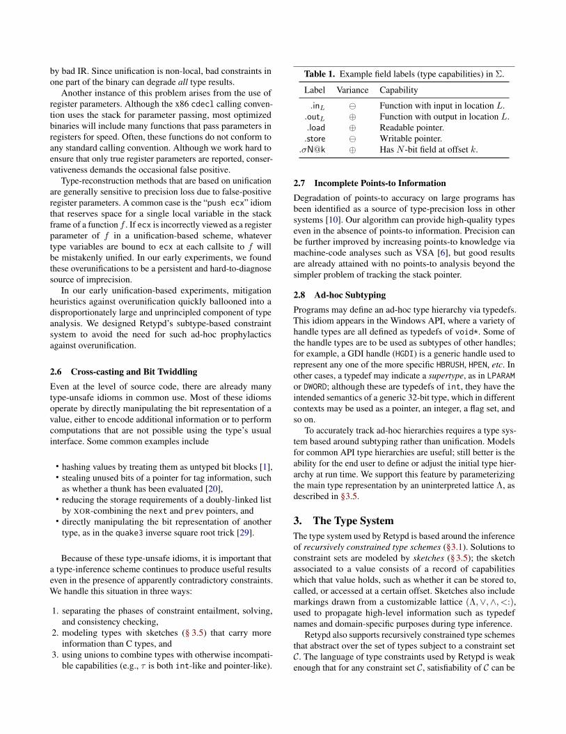
Table 1. Example field labels (type capabilities) in Σ.

Label Variance Capability

.inL Function with input in location L..outL ⊕ Function with output in location L..load ⊕ Readable pointer..store Writable pointer..σN@k ⊕ Has N -bit field at offset k.

2.7 Incomplete Points-to InformationDegradation of points-to accuracy on large programs hasbeen identified as a source of type-precision loss in othersystems [10]. Our algorithm can provide high-quality typeseven in the absence of points-to information. Precision canbe further improved by increasing points-to knowledge viamachine-code analyses such as VSA [6], but good resultsare already attained with no points-to analysis beyond thesimpler problem of tracking the stack pointer.

2.8 Ad-hoc SubtypingPrograms may define an ad-hoc type hierarchy via typedefs.This idiom appears in the Windows API, where a variety ofhandle types are all defined as typedefs of void*. Some ofthe handle types are to be used as subtypes of other handles;for example, a GDI handle (HGDI) is a generic handle used torepresent any one of the more specific HBRUSH, HPEN, etc. Inother cases, a typedef may indicate a supertype, as in LPARAMor DWORD; although these are typedefs of int, they have theintended semantics of a generic 32-bit type, which in differentcontexts may be used as a pointer, an integer, a flag set, andso on.

To accurately track ad-hoc hierarchies requires a type sys-tem based around subtyping rather than unification. Modelsfor common API type hierarchies are useful; still better is theability for the end user to define or adjust the initial type hier-archy at run time. We support this feature by parameterizingthe main type representation by an uninterpreted lattice Λ, asdescribed in §3.5.

3. The Type SystemThe type system used by Retypd is based around the inferenceof recursively constrained type schemes (§3.1). Solutions toconstraint sets are modeled by sketches (§3.5); the sketchassociated to a value consists of a record of capabilitieswhich that value holds, such as whether it can be stored to,called, or accessed at a certain offset. Sketches also includemarkings drawn from a customizable lattice (Λ,∨,∧, <:),used to propagate high-level information such as typedefnames and domain-specific purposes during type inference.

Retypd also supports recursively constrained type schemesthat abstract over the set of types subject to a constraint setC. The language of type constraints used by Retypd is weakenough that for any constraint set C, satisfiability of C can be

Derived Type Variable Formation

α v βVAR α

(T-LEFT)α v β, VAR α.`

VAR β.`(T-INHERITL)

α v βVAR β

(T-RIGHT)α v β, VAR β.`

VAR α.`(T-INHERITR)

VAR α.`

VAR α(T-PREFIX)

Subtyping

VAR α

α v α (S-REFL)α v β, VAR β.`, 〈`〉 = ⊕

α.` v β.` (S-FIELD⊕)

α v β, β v γα v γ (S-TRANS)

α v β, VAR β.`, 〈`〉 = β.` v α.` (S-FIELD)

VAR α.load, VAR α.store

α.store v α.load(S-POINTER)

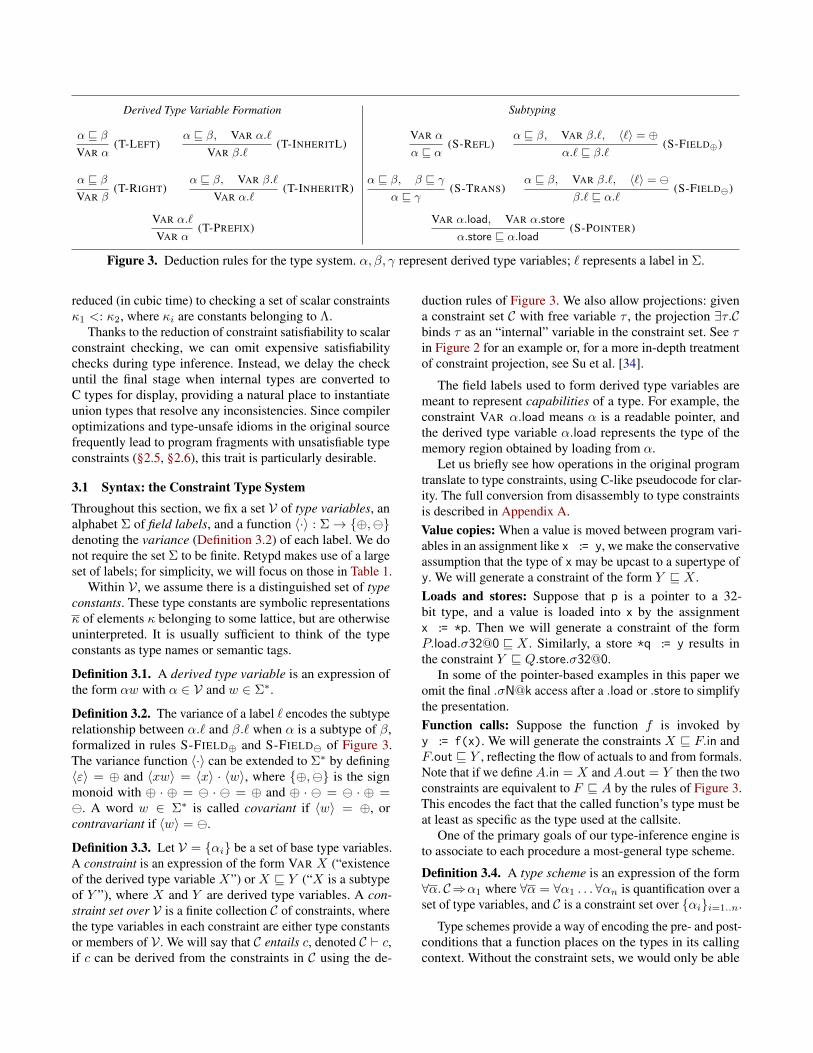
Figure 3. Deduction rules for the type system. α, β, γ represent derived type variables; ` represents a label in Σ.

reduced (in cubic time) to checking a set of scalar constraintsκ1 <: κ2, where κi are constants belonging to Λ.

Thanks to the reduction of constraint satisfiability to scalarconstraint checking, we can omit expensive satisfiabilitychecks during type inference. Instead, we delay the checkuntil the final stage when internal types are converted toC types for display, providing a natural place to instantiateunion types that resolve any inconsistencies. Since compileroptimizations and type-unsafe idioms in the original sourcefrequently lead to program fragments with unsatisfiable typeconstraints (§2.5, §2.6), this trait is particularly desirable.

3.1 Syntax: the Constraint Type SystemThroughout this section, we fix a set V of type variables, analphabet Σ of field labels, and a function 〈·〉 : Σ→ {⊕,}denoting the variance (Definition 3.2) of each label. We donot require the set Σ to be finite. Retypd makes use of a largeset of labels; for simplicity, we will focus on those in Table 1.

Within V , we assume there is a distinguished set of typeconstants. These type constants are symbolic representationsκ of elements κ belonging to some lattice, but are otherwiseuninterpreted. It is usually sufficient to think of the typeconstants as type names or semantic tags.

Definition 3.1. A derived type variable is an expression ofthe form αw with α ∈ V and w ∈ Σ∗.

Definition 3.2. The variance of a label ` encodes the subtyperelationship between α.` and β.` when α is a subtype of β,formalized in rules S-FIELD⊕ and S-FIELD of Figure 3.The variance function 〈·〉 can be extended to Σ∗ by defining〈ε〉 = ⊕ and 〈xw〉 = 〈x〉 · 〈w〉, where {⊕,} is the signmonoid with ⊕ · ⊕ = · = ⊕ and ⊕ · = · ⊕ =. A word w ∈ Σ∗ is called covariant if 〈w〉 = ⊕, orcontravariant if 〈w〉 = .

Definition 3.3. Let V = {αi} be a set of base type variables.A constraint is an expression of the form VAR X (“existenceof the derived type variable X”) or X v Y (“X is a subtypeof Y ”), where X and Y are derived type variables. A con-straint set over V is a finite collection C of constraints, wherethe type variables in each constraint are either type constantsor members of V . We will say that C entails c, denoted C ` c,if c can be derived from the constraints in C using the de-

duction rules of Figure 3. We also allow projections: givena constraint set C with free variable τ , the projection ∃τ.Cbinds τ as an “internal” variable in the constraint set. See τin Figure 2 for an example or, for a more in-depth treatmentof constraint projection, see Su et al. [34].

The field labels used to form derived type variables aremeant to represent capabilities of a type. For example, theconstraint VAR α.load means α is a readable pointer, andthe derived type variable α.load represents the type of thememory region obtained by loading from α.

Let us briefly see how operations in the original programtranslate to type constraints, using C-like pseudocode for clar-ity. The full conversion from disassembly to type constraintsis described in Appendix A.Value copies: When a value is moved between program vari-ables in an assignment like x := y, we make the conservativeassumption that the type of x may be upcast to a supertype ofy. We will generate a constraint of the form Y v X .Loads and stores: Suppose that p is a pointer to a 32-bit type, and a value is loaded into x by the assignmentx := *p. Then we will generate a constraint of the formP.load.σ32@0 v X . Similarly, a store *q := y results inthe constraint Y v Q.store.σ32@0.

In some of the pointer-based examples in this paper weomit the final .σN@k access after a .load or .store to simplifythe presentation.Function calls: Suppose the function f is invoked byy := f(x). We will generate the constraints X v F.in andF.out v Y , reflecting the flow of actuals to and from formals.Note that if we defineA.in = X andA.out = Y then the twoconstraints are equivalent to F v A by the rules of Figure 3.This encodes the fact that the called function’s type must beat least as specific as the type used at the callsite.

One of the primary goals of our type-inference engine isto associate to each procedure a most-general type scheme.

Definition 3.4. A type scheme is an expression of the form∀α. C⇒α1 where ∀α = ∀α1 . . . ∀αn is quantification over aset of type variables, and C is a constraint set over {αi}i=1..n.

Type schemes provide a way of encoding the pre- and post-conditions that a function places on the types in its callingcontext. Without the constraint sets, we would only be able

to represent conditions of the form “the input must be asubtype of X” and “the output must be a supertype of Y ”.The constraint set C can be used to encode more interestingtype relations between inputs and outputs, as in the caseof memcpy (§2.2). For example, a function that returns thesecond 4-byte element from a struct* may have the typescheme ∀τ. (τ.in.load.σ32@4 v τ.out)⇒τ .

3.2 Deduction RulesThe deduction rules for our type system appear in Figure 3.Most of the rules are self-evident under the interpretation inDefinition 3.3, but a few require some additional motivation.

S-FIELD⊕ and S-FIELD: These rules ensure that fieldlabels act as co- or contra-variant type operators, generat-ing subtype relations between derived type variables fromsubtype relations between the original variables.

T-INHERITL and T-INHERITR: The rule T-INHERITLshould be uncontroversial, since a subtype should have allcapabilities of its supertype. The rule T-INHERITR is moreunusual since it moves capabilities in the other direction;taken together, these rules require that two types in a subtyperelation must have exactly the same set of capabilities. Thisis a form of structural typing, ensuring that comparable typeshave the same shape.

Structural typing appears to be at odds with the need tocast more capable objects to less capable ones, as describedin §2.4. Indeed, T-INHERITR eliminates the possibility offorgetting capabilities during value assignments. But we stillmaintain this capability at procedure invocations due to ouruse of polymorphic type schemes. An explanation of howtype-scheme instantiation enables us to forget fields of anobject appears in §3.4, with more details in §E.1.2.

These rules ensure that Retypd can perform “iterativevariable recovery”; lack of iterative variable recovery wascited by the creators of the Phoenix decompiler [30] as acommon cause of incorrect decompilation when using TIE[17] for type recovery.

S-POINTER: This rule is a consistency condition ensuringthat the type that can be loaded from a pointer is a supertypeof the type that can be stored to a pointer. Without this rule,pointers would provide a channel for subverting the typesystem. An example of how this rule is used in practiceappears in §3.3.

The deduction rules of Figure 3 are simple enough thateach proof may be reduced to a normal form (see Theo-rem B.1). An encoding of the normal forms as transitionsequences in a modified pushdown system is used to pro-vide a compact representation of the entailment closureC = {c | C ` c}. The pushdown system modeling C isqueried and manipulated to provide most of the interestingtype-inference functionality. An outline of this functionalityappears in §5.2.

f() {p = q;

*p = x;y = *q;

}

g() {p = q;

*q = x;y = *p;

}

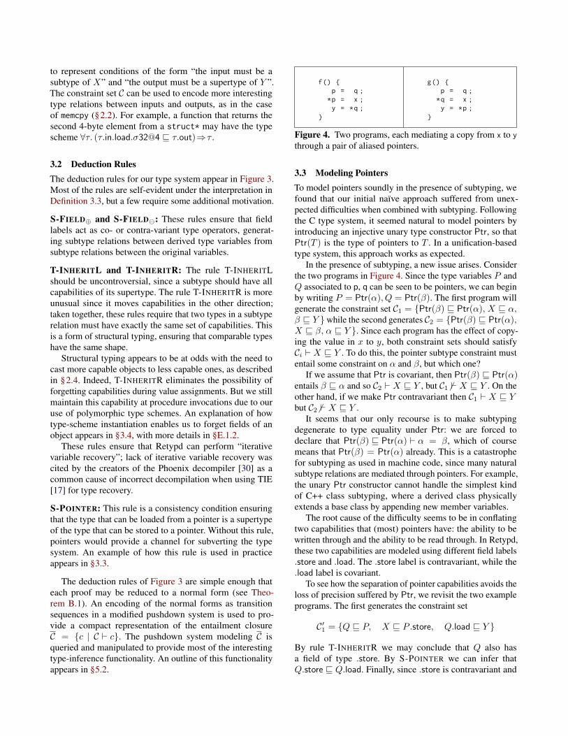
Figure 4. Two programs, each mediating a copy from x to y

through a pair of aliased pointers.

3.3 Modeling PointersTo model pointers soundly in the presence of subtyping, wefound that our initial naïve approach suffered from unex-pected difficulties when combined with subtyping. Followingthe C type system, it seemed natural to model pointers byintroducing an injective unary type constructor Ptr, so thatPtr(T ) is the type of pointers to T . In a unification-basedtype system, this approach works as expected.

In the presence of subtyping, a new issue arises. Considerthe two programs in Figure 4. Since the type variables P andQ associated to p, q can be seen to be pointers, we can beginby writing P = Ptr(α), Q = Ptr(β). The first program willgenerate the constraint set C1 = {Ptr(β) v Ptr(α), X v α,β v Y }while the second generates C2 = {Ptr(β) v Ptr(α),X v β, α v Y }. Since each program has the effect of copy-ing the value in x to y, both constraint sets should satisfyCi ` X v Y . To do this, the pointer subtype constraint mustentail some constraint on α and β, but which one?

If we assume that Ptr is covariant, then Ptr(β) v Ptr(α)entails β v α and so C2 ` X v Y , but C1 6 ` X v Y . On theother hand, if we make Ptr contravariant then C1 ` X v Ybut C2 6 ` X v Y .

It seems that our only recourse is to make subtypingdegenerate to type equality under Ptr: we are forced todeclare that Ptr(β) v Ptr(α) ` α = β, which of coursemeans that Ptr(β) = Ptr(α) already. This is a catastrophefor subtyping as used in machine code, since many naturalsubtype relations are mediated through pointers. For example,the unary Ptr constructor cannot handle the simplest kindof C++ class subtyping, where a derived class physicallyextends a base class by appending new member variables.

The root cause of the difficulty seems to be in conflatingtwo capabilities that (most) pointers have: the ability to bewritten through and the ability to be read through. In Retypd,these two capabilities are modeled using different field labels.store and .load. The .store label is contravariant, while the.load label is covariant.

To see how the separation of pointer capabilities avoids theloss of precision suffered by Ptr, we revisit the two exampleprograms. The first generates the constraint set

C′1 = {Q v P, X v P .store, Q.load v Y }

By rule T-INHERITR we may conclude that Q also hasa field of type .store. By S-POINTER we can infer thatQ.store v Q.load. Finally, since .store is contravariant and

Q v P , S-FIELD says we also have P .store v Q.store.Putting these parts together gives the subtype chain

X v P .store v Q.store v Q.load v Y

The second program generates the constraint set

C′2 = {Q v P, X v Q.store, P .load v Y }

Since Q v P and P has a field .load, we conclude that Qhas a .load field as well. Next, S-POINTER requires thatQ.store v Q.load. Since .load is covariant, Q v P impliesthat Q.load v P .load. This gives the subtype chain

X v Q.store v Q.load v P .load v Y

By splitting out the read- and write-capabilities of apointer, we can achieve a sound account of pointer subtypingthat does not degenerate to type equality. Note the importanceof the consistency condition S-POINTER: this rule ensuresthat writing through a pointer and reading the result cannotsubvert the type system.

The need for separate handling of read- and write-capabilities in a mutable reference has been rediscoveredmultiple times. A well-known instance is the covariance ofthe array type constructor in Java and C#, which can causeruntime type errors if the array is mutated; in these languages,the read capabilities are soundly modeled only by sacrificingsoundness for the write capabilities.

3.4 Non-structural Subtyping and T-INHERITRIt was noted in §3.2 that the rule T-INHERITR leads to asystem with a form of structural typing: any two types ina subtype relation must have the same capabilities. Super-ficially, this seems problematic for modeling typecasts thatforget about fields, such as a cast from derived* to base*when derived* has additional fields (§2.4).

The missing piece that allows us to effectively forget ca-pabilities is instantiation of callee type schemes at a callsite.To demonstrate how polymorphism enables forgetfulness,consider the example type scheme ∀F. (∃τ.C)⇒F from Fig-ure 2. The function close_last can be invoked by providingany actual-in type α, such that α v F.instack0; in particular,α can have more fields than those required by C. We simplyselect a more capable type for the existentially-quantifiedtype variable τ in C. In effect, we have used specialization ofpolymorphic types to model non-structural subtyping idioms,while subtyping is used only to model structural subtypingidioms. This restricts our introduction of non-structural sub-types to points where a type scheme is instantiated, such asat a call site.

3.5 Semantics: the Poset of SketchesThe simple type system defined by the deduction rules ofFigure 3 defines the syntax of legal derivations in our typesystem. The constraint solver of §5.2 is designed to find asimple representation for all conclusions that can be derived

>

>

α

>

>

β

A

A

instack0

outeax

loadσ3

2@0

σ32@4

loadα = int ∨#SuccessZ

β = int ∧#FileDescriptor

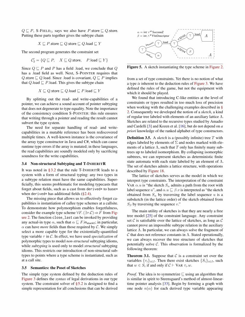
Figure 5. A sketch instantiating the type scheme in Figure 2.

from a set of type constraints. Yet there is no notion of whata type is inherent to the deduction rules of Figure 3. We havedefined the rules of the game, but not the equipment withwhich it should be played.

We found that introducing C-like entities at the level ofconstraints or types resulted in too much loss of precisionwhen working with the challenging examples described in §2. Consequently we developed the notion of a sketch, a kindof regular tree labeled with elements of an auxiliary lattice Λ.Sketches are related to the recursive types studied by Amadioand Cardelli [3] and Kozen et al. [16], but do not depend on apriori knowledge of the ranked alphabet of type constructors.

Definition 3.5. A sketch is a (possibly infinite) tree T withedges labeled by elements of Σ and nodes marked with ele-ments of a lattice Λ, such that T only has finitely many sub-trees up to labeled isomorphism. By collapsing isomorphicsubtrees, we can represent sketches as deterministic finitestate automata with each state labeled by an element of Λ.The set of sketches admits a lattice structure, with operationsdescribed by Figure 18.

The lattice of sketches serves as the model in which weinterpret type constraints. The interpretation of the constraintVAR α.u is “the sketch Sα admits a path from the root withlabel sequence u”, and α.u v β.v is interpreted as “the sketchobtained from Sα by traversing the label sequence u is asubsketch (in the lattice order) of the sketch obtained fromSβ by traversing the sequence v.”

The main utility of sketches is that they are nearly a freetree model [25] of the constraint language. Any constraintset C is satisfiable over the lattice of sketches, as long as Ccannot prove an impossible subtype relation in the auxiliarylattice Λ. In particular, we can always solve the fragment ofC that does not reference constants in Λ. Stated operationally,we can always recover the tree structure of sketches thatpotentially solve C. This observation is formalized by thefollowing theorem:

Theorem 3.1. Suppose that C is a constraint set over thevariables {τi}i∈I . Then there exist sketches {Si}i∈I , suchthat w ∈ Si if and only if C ` VAR τi.w.

Proof. The idea is to symmetrize v using an algorithm thatis similar in spirit to Steensgaard’s method of almost-linear-time pointer analysis [33]. Begin by forming a graph withone node n(α) for each derived type variable appearing

in C, along with each of its prefixes. Add a labeled edgen(α)

`→ n(α.`) for each derived type variable α.` to forma graph G. Now quotient G by the equivalence relation ∼defined by n(α) ∼ n(β) if α v β ∈ C, and n(α′) ∼ n(β′)

whenever there are edges n(α)`→ n(α′) and n(β)

`′→ n(β′)in G with n(α) ∼ n(β) where either ` = `′ or ` = .load and`′ = .store.

By construction, there exists a path through G/∼ withlabel sequence u starting at the equivalence class of τi if andonly if C ` VAR τi.u; the (regular) set of all such paths yieldsthe tree structure of Si.

Working out the lattice elements that should label Si is atrickier problem; the basic idea is to use the same automatonQ constructed during constraint simplification (Theorem 5.1)to answer queries about which type constants are upper andlower bounds on a given derived type variable. The fullalgorithm is listed in §D.4.

In Retypd, we use a large auxiliary lattice Λ containinghundreds of elements that includes a collection of standardC type names, common typedefs for popular APIs, anduser-specified semantic classes such as #FileDescriptor inFigure 2. This lattice helps model ad-hoc subtyping andpreserve high-level semantic type names, as discussed in§2.8.Note. Sketches are just one of many possible models for thededuction rules that could be proposed. A general approachis to fix a poset (T , <:) of types, interpret v as <:, andinterpret co- and contra-variant field labels as monotone (resp.antimonotone) functions T → T .

The separation of syntax from semantics allows for asimple way to parameterize the type-inference engine bya model of types. By choosing a model (T ,≡) with asymmetric relation ≡ ⊆ T × T , a unification-based typesystem similar to SecondWrite [10] is generated. On theother hand, by forming a lattice of type intervals and intervalinclusion, we would obtain a type system similar to TIE [17]that outputs upper and lower bounds on each type variable.

4. Analysis Framework4.1 IR ReconstructionRetypd is built on top of GrammaTech’s machine-code-analysis tool CodeSurfer for Binaries. CodeSurfer carriesout common program analyses on binaries for multiple CPUarchitectures, including x86, x86-64, and ARM. CodeSurferis used to recover a high-level IR from the raw machinecode; type constraints are generated directly from this IR, andresolved types are applied back to the IR and become visibleto the GUI and later analysis phases.

CodeSurfer achieves platform independence through TSL[18], a language for defining a processor’s concrete semanticsin terms of concrete numeric types and mapping types thatmodel flag, register, and memory banks. Interpreters fora given abstract domain are automatically created from

the concrete semantics simply by specifying the abstractdomain A and an interpretation of the concrete numeric andmapping types. Retypd uses CodeSurfer’s recovered IR todetermine the number and location of inputs and outputsto each procedure, as well as the program’s call graph andper-procedure control-flow graphs. An abstract interpreterthen generates sets of type constraints from the concreteTSL instruction semantics. A detailed account of the abstractsemantics for constraint generation appears in Appendix A.

4.2 Approach to Type ResolutionAfter the initial IR is recovered, type inference proceedsin two stages: first, type-constraint sets are generated in abottom-up fashion over the strongly-connected componentsof the callgraph. Pre-computed type schemes for externallylinked functions may be inserted at this stage. Each con-straint set is simplified by eliminating type variables that donot belong to the SCC’s interface; the simplification algo-rithm is outlined in § 5. Once type schemes are available,the callgraph is traversed bottom-up, assigning sketches totype variables as outlined in §3.5. During this stage, typeschemes are specialized based on the calling contexts of eachfunction. Appendix F lists the full algorithms for constraintsimplification (F.1) and solving (F.2).

4.3 Translation to C TypesThe final phase of type resolution converts the inferredsketches to C types for presentation to the user. Since Ctypes and sketches are not directly comparable, this resolu-tion phase necessarily involves the application of heuristicconversion policies. Restricting the heuristic policies to asingle post-inference phase provides us with the flexibility togenerate high-quality, human-readable C types while main-taining soundness and generality during type reconstruction.

Example 4.1. A simple example involves the generation ofconst annotations on pointers. We decided on a policy thatonly introduced const annotations on function parameters,by annotating the parameter at location L when the constraintset C for procedure p satisfies C ` VAR p.inL.load andC6 ` VAR p.inL.store. Retypd appears to be the first machine-code type-inference system to infer const annotations; acomparison of our recovered annotations to the originalsource code appears in §6.4.

Example 4.2. A more complex policy is used to decidebetween union types and generic types when incompatiblescalar constraints must be resolved. Retypd merges compara-ble scalar constraints to form antichains in Λ; the elements ofthese antichains are then used for the resulting C union type.

Example 4.3. The initial type-simplification stage results intypes that are as general as possible. Often, this means thattypes are found to be more general than is strictly helpfulto a (human) observer. A policy is applied that specializestype schemes to the most specific scheme that is compatiblewith all statically-discovered uses. For example, a C++ object

may include a getter function with a highly polymorphic typescheme, since it could operate equally well on any structurewith a field of the correct type at the correct offset. But weexpect that in every calling context, the getter will be calledon a specific object type (or perhaps its derived types). We canspecialize the getter’s type by choosing the least polymorphicspecialization that is compatible with the observed uses. Byspecializing the function signature before presenting a finalC type to the user, we trade some generality for types that aremore likely to match the original source.

5. The Simplification AlgorithmIn this section, we sketch an outline of the simplificationalgorithm at the core of the constraint solver. The completealgorithm appears in Appendix D.

5.1 Inferring a Type SchemeThe goal of the simplification algorithm is to take an inferredtype scheme ∀α.C⇒τ for a procedure and create a smallerconstraint set C′, such that any constraint on τ implied by Cis also implied by C′.

Let C denote the constraint set generated by abstractinterpretation of the procedure being analyzed, and let αbe the set of free type variables in C. We could alreadyuse ∀α. C ⇒ τ as the constraint set in the procedure’s typescheme, since the input and output types used in a validinvocation of f are tautologically those that satisfy C. Yet, asa practical matter, we cannot use the constraint set directly,since this would result in constraint sets with many uselessfree variables and a high growth rate over nested procedures.

Instead, we seek to generate a simplified constraint set C′,such that if c is an “interesting” constraint and C ` c thenC′ ` c as well. But what makes a constraint interesting?

Definition 5.1. For a type variable τ , a constraint is calledinteresting if it has one of the following forms:

• A capability constraint of the form VAR τ.u• A recursive subtype constraint of the form τ.u v τ.v• A subtype constraint of the form τ.u v κ or κ v τ.u

where κ is a type constant.

We will call a constraint set C′ a simplification of C if C′ ` cfor every interesting constraint c, such that C ` c. Since bothC and C′ entail the same set of constraints on τ , it is valid toreplace C with C′ in any valid type scheme for τ .

Simplification heuristics for set-constraint systems werestudied by Fähndrich and Aiken [12]; our simplificationalgorithm encompasses all of these heuristics.

5.2 Unconstrained Pushdown SystemsThe constraint-simplification algorithm works on a constraintset C by building a pushdown system PC whose transition se-quences represent valid derivations of subtyping judgements.We briefly review pushdown systems and some necessarygeneralizations here.

Definition 5.2. An unconstrained pushdown system is a tripleP = (V,Σ,∆) where V is the set of control locations,Σ is the set of stack symbols, and ∆ ⊆ (V × Σ∗)2 is a(possibly infinite) set of transition rules. We will denote atransition rule by 〈X;u〉 ↪→ 〈Y ; v〉 where X,Y ∈ V andu, v ∈ Σ∗. We define the set of configurations to be V × Σ∗.In a configuration (p, w), p is called the control state and wthe stack state.

Note that we require neither the set of stack symbols,nor the set of transition rules, to be finite. This freedom isrequired to model the derivation S-POINTER of Figure 3,which corresponds to an infinite set of transition rules.

Definition 5.3. An unconstrained pushdown system P de-termines a transition relation −→ on the set of configura-tions: (X,w) −→ (Y,w′) if there is a suffix s and a rule〈X;u〉 ↪→ 〈Y ; v〉, such that w = us and w′ = vs. Thetransitive closure of −→ is denoted ∗−→.

With this definition, we can state the primary theorembehind our simplification algorithm.

Theorem 5.1. Let C be a constraint set and V a set of basetype variables. Define a subset SC of (V ∪ Σ)∗ × (V ∪ Σ)∗

by (Xu, Y v) ∈ SC if and only if C ` X.u v Y.v. Then SCis a regular set, and an automaton Q to recognize SC can beconstructed in O(|C|3) time.

Proof. The basic idea is to treat each X.u v Y.v ∈ C as atransition rule 〈X;u〉 ↪→ 〈Y ; v〉 in the pushdown system P .In addition, we add control states #START,#END with tran-sitions 〈#START;X〉 ↪→ 〈X; ε〉 and 〈X; ε〉 ↪→ 〈#END;X〉for each X ∈ V . For the moment, assume that (1) all la-bels are covariant, and (2) the rule S-POINTER is ignored.By construction, (#START, Xu)

∗−→ (#END, Y v) in P ifand only if C ` X.u v Y.v. A theorem of Büchi [27] ensuresthat for any two control states A and B in a standard (notunconstrained) pushdown system, the set of all pairs (u, v)

with (A, u)∗−→ (B, v) is a regular language; Caucal [8]

gives a saturation algorithm that constructs an automaton torecognize this language.

In the full proof, we add two novelties: first, we supportcontravariant stack symbols by encoding variance data intothe control states and transition rules. The second noveltyinvolves the rule S-POINTER; this rule is problematic sincethe natural encoding would result in infinitely many transitionrules. We extend Caucal’s construction to lazily instantiateall necessary applications of S-POINTER during saturation.For details, see Appendix D.

Since C will usually entail an infinite number of con-straints, this theorem is particularly useful: it tells us thatthe full set of constraints entailed by C has a finite encodingby an automaton Q. Further manipulations on the constraintclosure, such as efficient minimization, can be carried outon Q. By restricting the transitions to and from #START and

#END, the same algorithm is used to eliminate type variables,producing the desired constraint simplifications.

5.3 Overall Complexity of InferenceThe saturation algorithm used to perform constraint-set sim-plification and type-scheme construction is, in the worst case,cubic in the number of subtype constraints to simplify. Sincesome well-known pointer analysis methods also have cubiccomplexity (such as Andersen [4]), it is reasonable to wonderif Retypd’s “points-to free” analysis really offers a benefitover a type-inference system built on top of points-to analysisdata.

To understand where Retypd’s efficiencies are found, firstconsider the n in O(n3). Retypd’s core saturation algorithmis cubic in the number of subtype constraints; due to thesimplicity of machine-code instructions, there is roughly onesubtype constraint generated per instruction. Furthermore,Retypd applies constraint simplification on each procedurein isolation to eliminate the procedure-local type variables,resulting in constraint sets that only relate procedure formal-ins, formal-outs, globals, and type constants. In practice, thesesimplified constraint sets are small.

Since each procedure’s constraint set is simplified inde-pendently, the n3 factor is controlled by the largest proceduresize, not the overall size of the binary. By contrast, source-code points-to analysis such as Andersen’s are generally cubicin the overall number of pointer variables, with exponentialduplication of variables depending on the call-string depthused for context sensitivity. The situation is even more diffi-cult for machine-code points-to analyses such as VSA, sincethere is no syntactic difference between a scalar and a pointerin machine code. In effect, every program variable must betreated as a potential pointer.

On our benchmark suite of real-world programs, we foundthat execution time for Retypd scales slightly belowO(N1.1),where N is the number of program instructions. The follow-ing back-of-the-envelope calculation can heuristically explainmuch of the disparity between the O(N3) theoretical com-plexity and theO(N1.1) measured complexity. On our bench-mark suite, the maximum procedure size n grew roughly liken ≈ N2/5. We could then expect that a per-procedure anal-ysis would perform worst when the program is partitionedintoN3/5 procedures of sizeN2/5. On such a program, a per-procedure O(nk) analysis may be expected to behave morelike anO(N3/5 ·(N2/5)k) = O(N (3+2k)/5) analysis overall.In particular, a per-procedure cubic analysis like Retypd couldbe expected to scale like a global O(N1.8) analysis. The re-maining differences in observed versus theoretical executiontime can be explained by the facts that real-world constraintgraphs do not tend to exercise the simplification algorithm’sworst-case behavior, and that the distribution of proceduresizes is heavily weighted towards small procedures.

INT_PTR Proto_EnumAccounts(WPARAM wParam ,LPARAM lParam)

{*( int* )wParam = accounts.getCount ();*( PROTOACCOUNT *** )lParam =

accounts.getArray ();return 0;

}

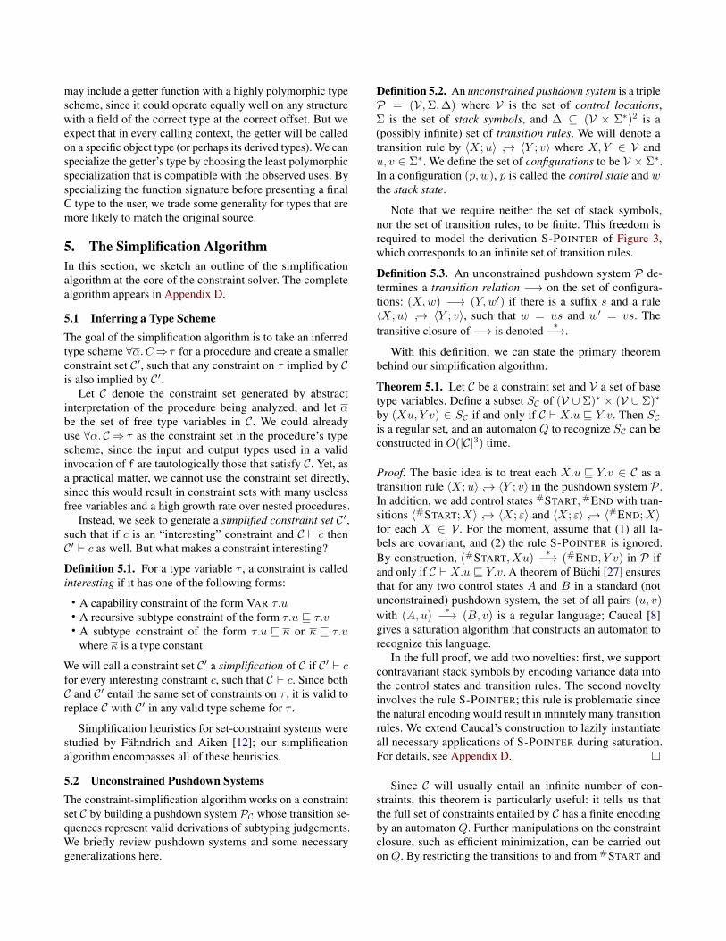
Figure 6. Ground-truth types declared in the original sourcedo not necessarily reflect program semantics. Example frommiranda32.

6. Evaluation6.1 ImplementationRetypd is implemented as a module within CodeSurferfor Binaries. By leveraging the multi-platform disassemblycapabilities of CodeSurfer, it can operate on x86, x86-64,and ARM code. We performed the evaluation using minimalanalysis settings, disabling value-set analysis (VSA) butcomputing affine relations between the stack and framepointers. Enabling additional CodeSurfer phases such as VSAcan greatly improve the reconstructed IR, at the expense ofincreased analysis time.

Existing type-inference algorithms such as TIE [17] andSecondWrite [10] require some modified form of VSA toresolve points-to data. Our approach shows that high-qualitytypes can be recovered in the absence of points-to informa-tion, allowing type inference to proceed even when comput-ing points-to data is too unreliable or expensive.

6.2 Evaluation SetupOur benchmark suite consists of 160 32-bit x86 binaries forboth Linux and Windows, compiled with a variety of gccand Microsoft Visual C/C++ versions. The benchmark suiteincludes a mix of executables, static libraries, and DLLs. Thesuite includes the same coreutils and SPEC2006 bench-marks used to evaluate REWARDS, TIE, and SecondWrite[10, 17, 19]; additional benchmarks came from a standardsuite of real-world programs used for precision and perfor-mance testing of CodeSurfer for Binaries. All binaries werebuilt with optimizations enabled and debug information dis-abled.

Ground truth is provided by separate copies of the binariesthat have been built with the same settings, but with debuginformation included (DWARF on Linux, PDB on Windows).We used IdaPro [15] to read the debug information, whichallowed us to use the same scripts for collecting ground-truthtypes from both DWARF and PDB data.

All benchmarks were evaluated on a 2.6 GHz Intel XeonE5-2670 CPU, running on a single logical core. RAM uti-lization by CodeSurfer and Retypd combined was capped at10GB.

Benchmark Description Instructions

CodeSurfer benchmarks

libidn Domain name translator 7KTutorial00 Direct3D tutorial 9Kzlib Compression library 14Kogg Multimedia library 20Kdistributor UltraVNC repeater 22Klibbz2 BZIP library, as a DLL 37Kglut The glut32.dll library 40Kpngtest A test of libpng 42Kfreeglut The freeglut.dll library 77Kmiranda IRC client 100KXMail Email server 137Kyasm Modular assembler 190Kpython21 Python 2.1 202Kquake3 Quake 3 281KTinyCad Computed-aided design 544KShareaza Peer-to-peer file sharing 842K

SPEC2006 benchmarks

470.lbm Lattice Boltzmann Method 3K429.mcf Vehicle scheduling 3K462.libquantum Quantum computation 11K401.bzip2 Compression 13K458.sjeng Chess AI 25K433.milc Quantum field theory 28K482.sphinx3 Speech recognition 43K456.hmmer Protein sequence analysis 71K464.h264ref Video compression 113K445.gobmk GNU Go AI 203K400.perlbench Perl core 261K403.gcc C/C++/Fortran compiler 751K

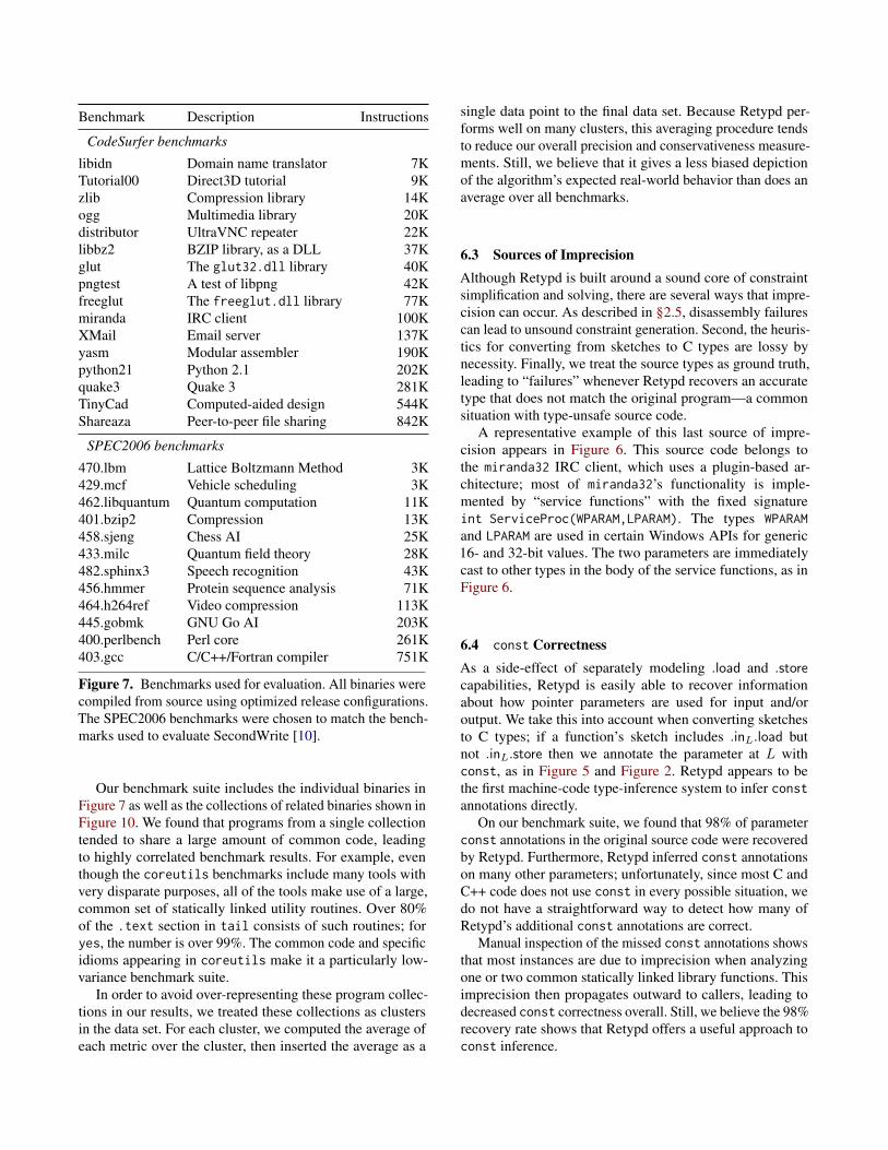
Figure 7. Benchmarks used for evaluation. All binaries werecompiled from source using optimized release configurations.The SPEC2006 benchmarks were chosen to match the bench-marks used to evaluate SecondWrite [10].

Our benchmark suite includes the individual binaries inFigure 7 as well as the collections of related binaries shown inFigure 10. We found that programs from a single collectiontended to share a large amount of common code, leadingto highly correlated benchmark results. For example, eventhough the coreutils benchmarks include many tools withvery disparate purposes, all of the tools make use of a large,common set of statically linked utility routines. Over 80%of the .text section in tail consists of such routines; foryes, the number is over 99%. The common code and specificidioms appearing in coreutils make it a particularly low-variance benchmark suite.

In order to avoid over-representing these program collec-tions in our results, we treated these collections as clustersin the data set. For each cluster, we computed the average ofeach metric over the cluster, then inserted the average as a

single data point to the final data set. Because Retypd per-forms well on many clusters, this averaging procedure tendsto reduce our overall precision and conservativeness measure-ments. Still, we believe that it gives a less biased depictionof the algorithm’s expected real-world behavior than does anaverage over all benchmarks.

6.3 Sources of ImprecisionAlthough Retypd is built around a sound core of constraintsimplification and solving, there are several ways that impre-cision can occur. As described in §2.5, disassembly failurescan lead to unsound constraint generation. Second, the heuris-tics for converting from sketches to C types are lossy bynecessity. Finally, we treat the source types as ground truth,leading to “failures” whenever Retypd recovers an accuratetype that does not match the original program—a commonsituation with type-unsafe source code.

A representative example of this last source of impre-cision appears in Figure 6. This source code belongs tothe miranda32 IRC client, which uses a plugin-based ar-chitecture; most of miranda32’s functionality is imple-mented by “service functions” with the fixed signatureint ServiceProc(WPARAM,LPARAM). The types WPARAMand LPARAM are used in certain Windows APIs for generic16- and 32-bit values. The two parameters are immediatelycast to other types in the body of the service functions, as inFigure 6.

6.4 const CorrectnessAs a side-effect of separately modeling .load and .storecapabilities, Retypd is easily able to recover informationabout how pointer parameters are used for input and/oroutput. We take this into account when converting sketchesto C types; if a function’s sketch includes .inL.load butnot .inL.store then we annotate the parameter at L withconst, as in Figure 5 and Figure 2. Retypd appears to bethe first machine-code type-inference system to infer constannotations directly.

On our benchmark suite, we found that 98% of parameterconst annotations in the original source code were recoveredby Retypd. Furthermore, Retypd inferred const annotationson many other parameters; unfortunately, since most C andC++ code does not use const in every possible situation, wedo not have a straightforward way to detect how many ofRetypd’s additional const annotations are correct.

Manual inspection of the missed const annotations showsthat most instances are due to imprecision when analyzingone or two common statically linked library functions. Thisimprecision then propagates outward to callers, leading todecreased const correctness overall. Still, we believe the 98%recovery rate shows that Retypd offers a useful approach toconst inference.

TIE

REWARDS-c* TIE*

Retypd

0

0.5

1

1.5

2coreutils

Secon

dWrit

e

Retypd

SPEC2006

Retypd

0

0.5

1

1.5

2All

Distance to source type Interval size

∗ Dynamic

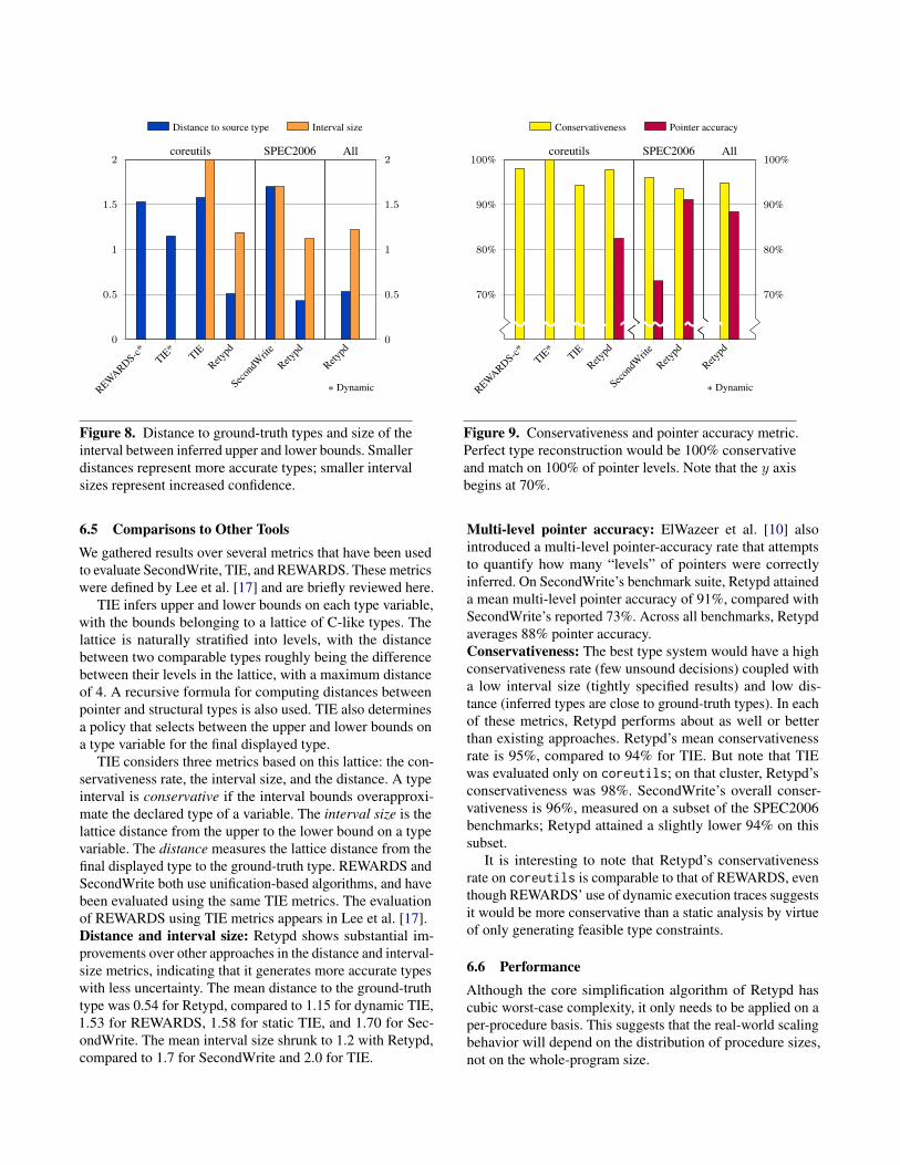
Figure 8. Distance to ground-truth types and size of theinterval between inferred upper and lower bounds. Smallerdistances represent more accurate types; smaller intervalsizes represent increased confidence.

TIE

REWARDS-c* TIE*

Retypd

70%

80%

90%

100%coreutils

Secon

dWrit

e

Retypd

SPEC2006

Retypd

70%

80%

90%

100%All

Conservativeness Pointer accuracy

∗ Dynamic

Figure 9. Conservativeness and pointer accuracy metric.Perfect type reconstruction would be 100% conservativeand match on 100% of pointer levels. Note that the y axisbegins at 70%.

6.5 Comparisons to Other ToolsWe gathered results over several metrics that have been usedto evaluate SecondWrite, TIE, and REWARDS. These metricswere defined by Lee et al. [17] and are briefly reviewed here.

TIE infers upper and lower bounds on each type variable,with the bounds belonging to a lattice of C-like types. Thelattice is naturally stratified into levels, with the distancebetween two comparable types roughly being the differencebetween their levels in the lattice, with a maximum distanceof 4. A recursive formula for computing distances betweenpointer and structural types is also used. TIE also determinesa policy that selects between the upper and lower bounds ona type variable for the final displayed type.

TIE considers three metrics based on this lattice: the con-servativeness rate, the interval size, and the distance. A typeinterval is conservative if the interval bounds overapproxi-mate the declared type of a variable. The interval size is thelattice distance from the upper to the lower bound on a typevariable. The distance measures the lattice distance from thefinal displayed type to the ground-truth type. REWARDS andSecondWrite both use unification-based algorithms, and havebeen evaluated using the same TIE metrics. The evaluationof REWARDS using TIE metrics appears in Lee et al. [17].Distance and interval size: Retypd shows substantial im-provements over other approaches in the distance and interval-size metrics, indicating that it generates more accurate typeswith less uncertainty. The mean distance to the ground-truthtype was 0.54 for Retypd, compared to 1.15 for dynamic TIE,1.53 for REWARDS, 1.58 for static TIE, and 1.70 for Sec-ondWrite. The mean interval size shrunk to 1.2 with Retypd,compared to 1.7 for SecondWrite and 2.0 for TIE.

Multi-level pointer accuracy: ElWazeer et al. [10] alsointroduced a multi-level pointer-accuracy rate that attemptsto quantify how many “levels” of pointers were correctlyinferred. On SecondWrite’s benchmark suite, Retypd attaineda mean multi-level pointer accuracy of 91%, compared withSecondWrite’s reported 73%. Across all benchmarks, Retypdaverages 88% pointer accuracy.Conservativeness: The best type system would have a highconservativeness rate (few unsound decisions) coupled witha low interval size (tightly specified results) and low dis-tance (inferred types are close to ground-truth types). In eachof these metrics, Retypd performs about as well or betterthan existing approaches. Retypd’s mean conservativenessrate is 95%, compared to 94% for TIE. But note that TIEwas evaluated only on coreutils; on that cluster, Retypd’sconservativeness was 98%. SecondWrite’s overall conser-vativeness is 96%, measured on a subset of the SPEC2006benchmarks; Retypd attained a slightly lower 94% on thissubset.

It is interesting to note that Retypd’s conservativenessrate on coreutils is comparable to that of REWARDS, eventhough REWARDS’ use of dynamic execution traces suggestsit would be more conservative than a static analysis by virtueof only generating feasible type constraints.

6.6 PerformanceAlthough the core simplification algorithm of Retypd hascubic worst-case complexity, it only needs to be applied on aper-procedure basis. This suggests that the real-world scalingbehavior will depend on the distribution of procedure sizes,not on the whole-program size.

Cluster Count Description Instructions Distance Interval Conserv. Ptr. Acc. Const

freeglut-demos 3 freeglut samples 2K 0.66 1.49 97% 83% 100%coreutils 107 GNU coreutils 8.23 10K 0.51 1.19 98% 82% 96%vpx-d 8 VPx decoders 36K 0.63 1.68 98% 92% 100%vpx-e 6 VPx encoders 78K 0.63 1.53 96% 90% 100%sphinx2 4 Speech recognition 83K 0.42 1.09 94% 91% 99%putty 4 SSH utilities 97K 0.51 1.05 94% 86% 99%

Retypd, as reported 0.54 1.20 95% 88% 98%Retypd, without clustering 0.53 1.22 97% 84% 97%

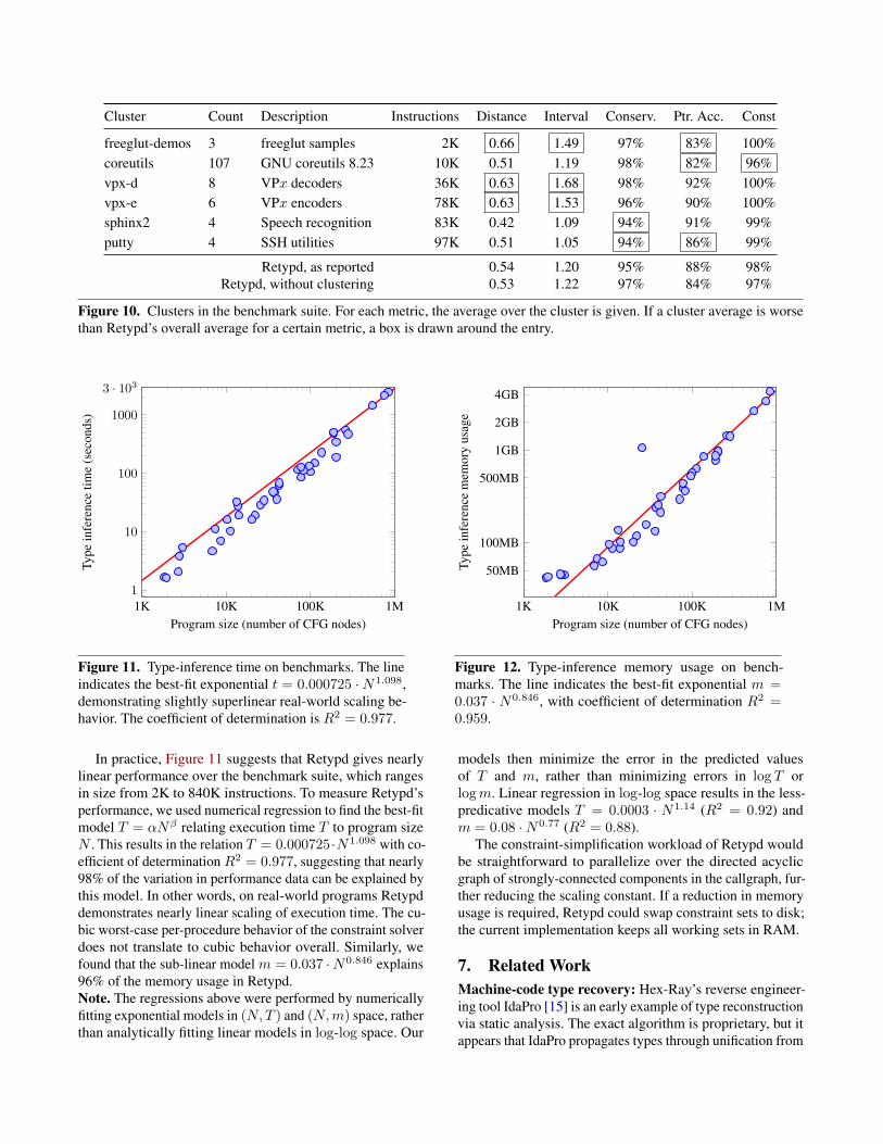
Figure 10. Clusters in the benchmark suite. For each metric, the average over the cluster is given. If a cluster average is worsethan Retypd’s overall average for a certain metric, a box is drawn around the entry.

1

10

100

1000

1K 10K 100K 1M

3 · 103

Program size (number of CFG nodes)

Type

infe

renc

etim

e(s

econ

ds)

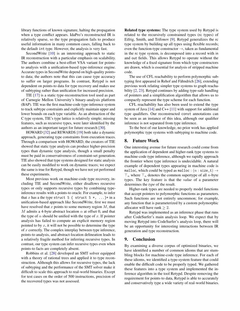
Figure 11. Type-inference time on benchmarks. The lineindicates the best-fit exponential t = 0.000725 ·N1.098,demonstrating slightly superlinear real-world scaling be-havior. The coefficient of determination is R2 = 0.977.

1K 10K 100K 1M

50MB

100MB

500MB

1GB

2GB

4GB

Program size (number of CFG nodes)

Type

infe

renc

em

emor

yus

age

Figure 12. Type-inference memory usage on bench-marks. The line indicates the best-fit exponential m =0.037 · N0.846, with coefficient of determination R2 =0.959.

In practice, Figure 11 suggests that Retypd gives nearlylinear performance over the benchmark suite, which rangesin size from 2K to 840K instructions. To measure Retypd’sperformance, we used numerical regression to find the best-fitmodel T = αNβ relating execution time T to program sizeN . This results in the relation T = 0.000725·N1.098 with co-efficient of determination R2 = 0.977, suggesting that nearly98% of the variation in performance data can be explained bythis model. In other words, on real-world programs Retypddemonstrates nearly linear scaling of execution time. The cu-bic worst-case per-procedure behavior of the constraint solverdoes not translate to cubic behavior overall. Similarly, wefound that the sub-linear model m = 0.037 ·N0.846 explains96% of the memory usage in Retypd.Note. The regressions above were performed by numericallyfitting exponential models in (N,T ) and (N,m) space, ratherthan analytically fitting linear models in log-log space. Our

models then minimize the error in the predicted valuesof T and m, rather than minimizing errors in log T orlogm. Linear regression in log-log space results in the less-predicative models T = 0.0003 · N1.14 (R2 = 0.92) andm = 0.08 ·N0.77 (R2 = 0.88).

The constraint-simplification workload of Retypd wouldbe straightforward to parallelize over the directed acyclicgraph of strongly-connected components in the callgraph, fur-ther reducing the scaling constant. If a reduction in memoryusage is required, Retypd could swap constraint sets to disk;the current implementation keeps all working sets in RAM.

7. Related WorkMachine-code type recovery: Hex-Ray’s reverse engineer-ing tool IdaPro [15] is an early example of type reconstructionvia static analysis. The exact algorithm is proprietary, but itappears that IdaPro propagates types through unification from

library functions of known signature, halting the propagationwhen a type conflict appears. IdaPro’s reconstructed IR isrelatively sparse, so the type propagation fails to produceuseful information in many common cases, falling back tothe default int type. However, the analysis is very fast.

SecondWrite [10] is an interesting approach to staticIR reconstruction with a particular emphasis on scalability.The authors combine a best-effort VSA variant for points-to analysis with a unification-based type-inference engine.Accurate types in SecondWrite depend on high-quality points-to data; the authors note that this can cause type accuracyto suffer on larger programs. In contrast, Retypd is notdependent on points-to data for type recovery and makes useof subtyping rather than unification for increased precision.

TIE [17] is a static type-reconstruction tool used as partof Carnegie Mellon University’s binary-analysis platform(BAP). TIE was the first machine-code type-inference systemto track subtype constraints and explicitly maintain upper andlower bounds on each type variable. As an abstraction of theC type system, TIE’s type lattice is relatively simple; missingfeatures, such as recursive types, were later identified by theauthors as an important target for future research [30].

HOWARD [32] and REWARDS [19] both take a dynamicapproach, generating type constraints from execution traces.Through a comparison with HOWARD, the creators of TIEshowed that static type analysis can produce higher-precisiontypes than dynamic type analysis, though a small penaltymust be paid in conservativeness of constraint-set generation.TIE also showed that type systems designed for static analysiscan be easily modified to work on dynamic traces; we expectthe same is true for Retypd, though we have not yet performedthese experiments.

Most previous work on machine-code type recovery, in-cluding TIE and SecondWrite, either disallows recursivetypes or only supports recursive types by combining type-inference results with a points-to oracle. For example, to inferthat x has a the type struct S { struct S *, ...}* in aunification-based approach like SecondWrite, first we musthave resolved that x points to some memory region M , thatM admits a 4-byte abstract location α at offset 0, and thatthe type of α should be unified with the type of x. If pointeranalysis has failed to compute an explicit memory regionpointed to by x, it will not be possible to determine the typeof x correctly. The complex interplay between type inference,points-to analysis, and abstract-location delineation leads toa relatively fragile method for inferring recursive types. Incontrast, our type system can infer recursive types even whenpoints-to facts are completely absent.

Robbins et al. [28] developed an SMT solver equippedwith a theory of rational trees and applied it to type recon-struction. Although this allows for recursive types, the lackof subtyping and the performance of the SMT solver make itdifficult to scale this approach to real-world binaries. Exceptfor test cases on the order of 500 instructions, precision ofthe recovered types was not assessed.

Related type systems: The type system used by Retypd isrelated to the recursively constrained types (rc types) ofEifrig, Smith, and Trifonov [9]. Retypd generalizes the rctype system by building up all types using flexible records;even the function-type constructor→, taken as fundamentalin the rc type system, is decomposed into a record with inand out fields. This allows Retypd to operate without theknowledge of a fixed signature from which type constructorsare drawn, which is essential for analysis of stripped machinecode.

The use of CFL reachability to perform polymorphic sub-typing first appeared in Rehof and Fähndrich [26], extendingprevious work relating simpler type systems to graph reacha-bility [2, 23]. Retypd continues by adding type-safe handlingof pointers and a simplification algorithm that allows us tocompactly represent the type scheme for each function.

CFL reachability has also been used to extend the typesystem of Java [14] and C++ [11] with support for additionaltype qualifiers. Our reconstructed const annotations canbe seen as an instance of this idea, although our qualifierinference is not separated from type inference.

To the best of our knowledge, no prior work has appliedpolymorphic type systems with subtyping to machine code.

8. Future WorkOne interesting avenue for future research could come fromthe application of dependent and higher-rank type systems tomachine-code type inference, although we rapidly approachthe frontier where type inference is undecidable. A naturalexample of dependent types appearing in machine code ismalloc, which could be typed as malloc : (n : size_t)→>n where >n denotes the common supertype of all n-bytetypes. The key feature is that the value of a parameterdetermines the type of the result.

Higher-rank types are needed to properly model functionsthat accept pointers to polymorphic functions as parameters.Such functions are not entirely uncommon; for example,any function that is parameterized by a custom polymorphicallocator will have rank ≥ 2.

Retypd was implemented as an inference phase that runsafter CodeSurfer’s main analysis loop. We expect that bymoving Retypd into CodeSurfer’s analysis loop, there willbe an opportunity for interesting interactions between IRgeneration and type reconstruction.

9. ConclusionBy examining a diverse corpus of optimized binaries, wehave identified a number of common idioms that are stum-bling blocks for machine-code type inference. For each ofthese idioms, we identified a type-system feature that couldenable the difficult code to be properly typed. We gatheredthese features into a type system and implemented the in-ference algorithm in the tool Retypd. Despite removing therequirement for points-to data, Retypd is able to accuratelyand conservatively type a wide variety of real-world binaries.

We assert that Retypd demonstrates the utility of high-leveltype systems for reverse engineering and binary analysis.

AcknowledgmentsThe authors would like to thank Vineeth Kashyap and theanonymous reviewers for their many useful comments on thismanuscript, and John Phillips, David Ciarletta, and Tim Clarkfor their help with test automation.

References[1] ISO/IEC TR 19768:2007: Technical report on C++ library

extensions, 2007.

[2] O. Agesen. Constraint-based type inference and parametricpolymorphism. In Static Analysis Symposium, pages 78–100,1994.

[3] R. M. Amadio and L. Cardelli. Subtyping recursive types.ACM Transactions on Programming Languages and Systems,15(4):575–631, 1993.

[4] L. O. Andersen. Program analysis and specialization forthe C programming language. PhD thesis, University ofCophenhagen, 1994.

[5] G. Balakrishnan, R. Gruian, T. Reps, and T. Teitelbaum.CodeSurfer/x86 – a platform for analyzing x86 executables. InCompiler Construction, pages 250–254, 2005.

[6] G. Balakrishnan and T. Reps. Analyzing Memory Accesses inx86 Executables, in Compiler Construction, pages 5–23, 2004.

[7] A. Carayol and M. Hague. Saturation algorithms for model-checking pushdown systems. In International Conference onAutomata and Formal Languages, pages 1–24, 2014.

[8] D. Caucal. On the regular structure of prefix rewriting. Theo-retical Computer Science, 106(1):61–86, 1992.

[9] J. Eifrig, S. Smith, and V. Trifonov. Sound polymorphictype inference for objects. In Object-Oriented Programming,Systems, Languages, and Applications, pages 169–184, 1995.

[10] K. ElWazeer, K. Anand, A. Kotha, M. Smithson, and R. Barua.Scalable variable and data type detection in a binary rewriter.In Programming Language Design and Implementation, pages51–60, 2013.

[11] J. S. Foster, R. Johnson, J. Kodumal, and A. Aiken. Flow-insensitive type qualifiers. ACM Transactions on ProgrammingLanguages and Systems, 28(6):1035–1087, 2006.

[12] M. Fähndrich and A. Aiken. Making set-constraint programanalyses scale. In Workshop on Set Constraints, 1996.

[13] D. Gopan, E. Driscoll, D. Nguyen, D. Naydich, A. Loginov,and D. Melski. Data-delineation in software binaries andits application to buffer-overrun discovery. In InternationalConference on Software Engineering, pages 145–155, 2015.

[14] D. Greenfieldboyce and J. S. Foster. Type qualifier inference forJava. In Object-Oriented Programming, Systems, Languages,and Applications, pages 321–336, 2007.

[15] Hex-Rays. Hex-Rays IdaPro. http://www.hex-rays.com/products/ida/, 2015.

[16] D. Kozen, J. Palsberg, and M. I. Schwartzbach. Efficientrecursive subtyping. Mathematical Structures in ComputerScience, 5(01):113–125, 1995.

[17] J. Lee, T. Avgerinos, and D. Brumley. TIE: Principled reverseengineering of types in binary programs. In Network andDistributed System Security Symposium, pages 251–268, 2011.

[18] J. Lim and T. Reps. TSL: A system for generating abstractinterpreters and its application to machine-code analysis. ACMTransactions on Programming Languages and Systems , 35(1):4, 2013.

[19] Z. Lin, X. Zhang, and D. Xu. Automatic reverse engineeringof data structures from binary execution. In Network andDistributed System Security Symposium, 2010.

[20] S. Marlow, A. R. Yakushev, and S. Peyton Jones. Faster lazi-ness using dynamic pointer tagging. In International Confer-ence on Functional Programming, pages 277–288, 2007.

[21] L. Mauborgne and X. Rival. Trace partitioning in abstract inter-pretation based static analyzers. In Programming Languagesand Systems, pages 5–20, 2005.

[22] M. Noonan, A. Loginov, and D. Cok. Polymorphic typeinference for machine code (extended version). URL http://arxiv.org/abs/1603.05495.

[23] J. Palsberg and P. O’Keefe. A type system equivalent to flowanalysis. ACM Transactions on Programming Languages andSystems , 17(4):576–599, 1995.

[24] J. Palsberg, M. Wand, and P. O’Keefe. Type inference withnon-structural subtyping. Formal Aspects of Computing, 9(1):49–67, 1997.

[25] F. Pottier and D. Rémy. The essence of ML type inference. InB. C. Pierce, editor, Advanced Topics in Types and Program-ming Languages, chapter 10. MIT Press, 2005.

[26] J. Rehof and M. Fähndrich. Type-based flow analysis: Frompolymorphic subtyping to cfl-reachability. In Principles ofProgramming Languages, pages 54–66, 2001.

[27] J. Richard Büchi. Regular canonical systems. Archive forMathematical Logic, 6(3):91–111, 1964.

[28] E. Robbins, J. M. Howe, and A. King. Theory propagationand rational-trees. In Principles and Practice of DeclarativeProgramming, pages 193–204, 2013.

[29] M. Robertson. A Brief History of InvSqrt. PhD thesis,University of New Brunswick, 2012.

[30] E. J. Schwartz, J. Lee, M. Woo, and D. Brumley. Native x86decompilation using semantics-preserving structural analysisand iterative control-flow structuring. In USENIX SecuritySymposium, pages 353–368, 2013.

[31] M. Siff, S. Chandra, T. Ball, K. Kunchithapadam, andT. Reps. Coping with type casts in C. In Software Engi-neering—ESEC/FSE’99, pages 180–198, 1999.

[32] A. Slowinska, T. Stancescu, and H. Bos. Howard: A dynamicexcavator for reverse engineering data structures. In Networkand Distributed System Security Symposium, 2011.

[33] B. Steensgaard. Points-to analysis in almost linear time. InPrinciples of Programming Languages, pages 32–41, 1996.

[34] Z. Su, A. Aiken, J. Niehren, T. Priesnitz, and R. Treinen. Thefirst-order theory of subtyping constraints. In Principles ofProgramming Languages, pages 203–216, 2002.

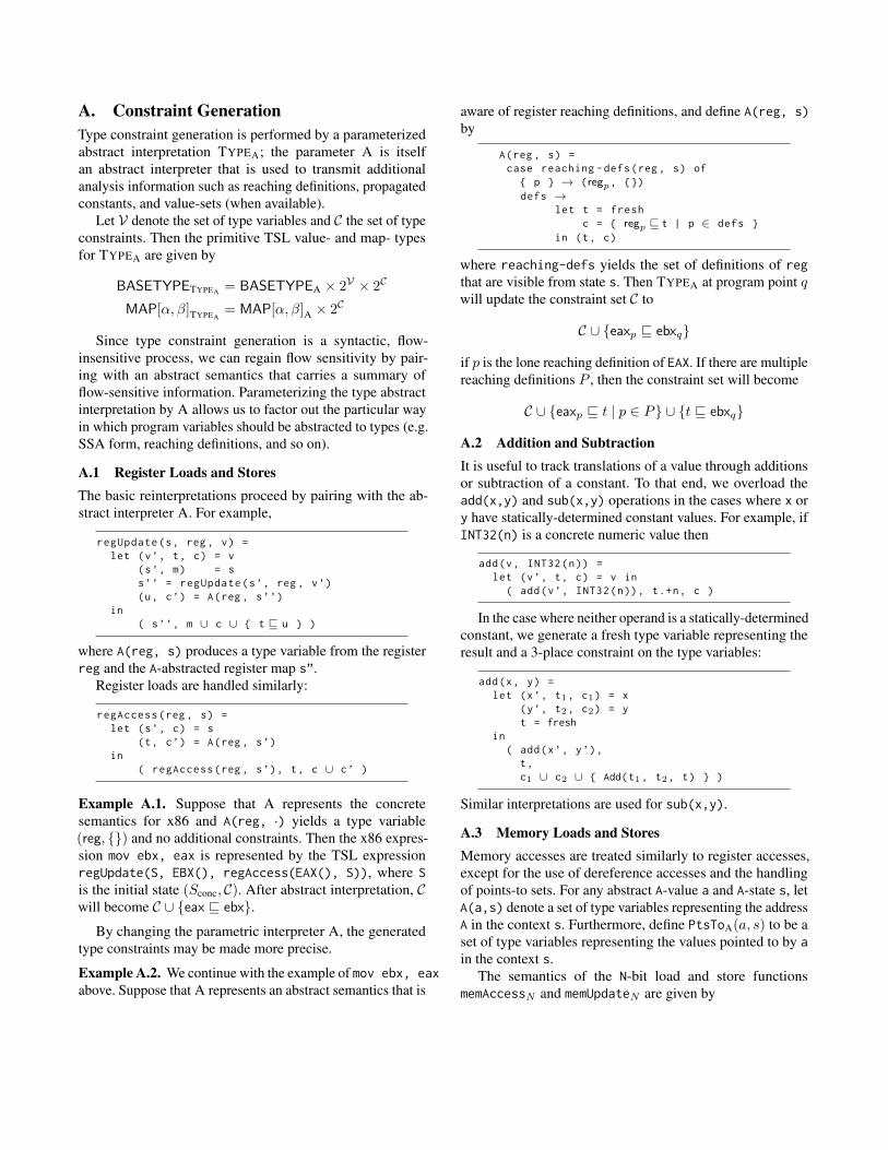
A. Constraint GenerationType constraint generation is performed by a parameterizedabstract interpretation TYPEA; the parameter A is itselfan abstract interpreter that is used to transmit additionalanalysis information such as reaching definitions, propagatedconstants, and value-sets (when available).

Let V denote the set of type variables and C the set of typeconstraints. Then the primitive TSL value- and map- typesfor TYPEA are given by

BASETYPETYPEA = BASETYPEA × 2V × 2C

MAP[α, β]TYPEA= MAP[α, β]A × 2C

Since type constraint generation is a syntactic, flow-insensitive process, we can regain flow sensitivity by pair-ing with an abstract semantics that carries a summary offlow-sensitive information. Parameterizing the type abstractinterpretation by A allows us to factor out the particular wayin which program variables should be abstracted to types (e.g.SSA form, reaching definitions, and so on).

A.1 Register Loads and StoresThe basic reinterpretations proceed by pairing with the ab-stract interpreter A. For example,

regUpdate(s, reg , v) =let (v’, t, c) = v

(s’, m) = ss’’ = regUpdate(s’, reg , v’)(u, c’) = A(reg , s’’)

in( s’’, m ∪ c ∪ { t v u } )

where A(reg, s) produces a type variable from the registerreg and the A-abstracted register map s”.

Register loads are handled similarly:

regAccess(reg , s) =let (s’, c) = s

(t, c’) = A(reg , s’)in

( regAccess(reg , s’), t, c ∪ c’ )

Example A.1. Suppose that A represents the concretesemantics for x86 and A(reg, ·) yields a type variable(reg, {}) and no additional constraints. Then the x86 expres-sion mov ebx, eax is represented by the TSL expressionregUpdate(S, EBX(), regAccess(EAX(), S)), where Sis the initial state (Sconc, C). After abstract interpretation, Cwill become C ∪ {eax v ebx}.

By changing the parametric interpreter A, the generatedtype constraints may be made more precise.

Example A.2. We continue with the example of mov ebx, eaxabove. Suppose that A represents an abstract semantics that is

aware of register reaching definitions, and define A(reg, s)by

A(reg , s) =case reaching -defs(reg , s) of

{ p } → (regp, {})defs →

let t = freshc = { regp v t | p ∈ defs }

in (t, c)

where reaching-defs yields the set of definitions of regthat are visible from state s. Then TYPEA at program point qwill update the constraint set C to

C ∪ {eaxp v ebxq}

if p is the lone reaching definition of EAX. If there are multiplereaching definitions P , then the constraint set will become

C ∪ {eaxp v t | p ∈ P} ∪ {t v ebxq}

A.2 Addition and SubtractionIt is useful to track translations of a value through additionsor subtraction of a constant. To that end, we overload theadd(x,y) and sub(x,y) operations in the cases where x ory have statically-determined constant values. For example, ifINT32(n) is a concrete numeric value then

add(v, INT32(n)) =let (v’, t, c) = v in

( add(v’, INT32(n)), t.+n, c )

In the case where neither operand is a statically-determinedconstant, we generate a fresh type variable representing theresult and a 3-place constraint on the type variables:

add(x, y) =let (x’, t1, c1) = x

(y’, t2, c2) = yt = fresh

in( add(x’, y’),

t,c1 ∪ c2 ∪ { Add(t1, t2, t) } )

Similar interpretations are used for sub(x,y).

A.3 Memory Loads and StoresMemory accesses are treated similarly to register accesses,except for the use of dereference accesses and the handlingof points-to sets. For any abstract A-value a and A-state s, letA(a,s) denote a set of type variables representing the addressA in the context s. Furthermore, define PtsToA(a, s) to be aset of type variables representing the values pointed to by ain the context s.

The semantics of the N-bit load and store functionsmemAccessN and memUpdateN are given by

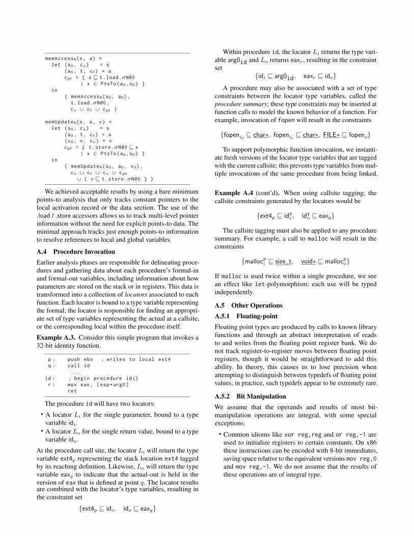
memAccessN(s, a) =let (s0, cs) = s

(a0, t, ct) = acpt = { x v t.load.σN@0

| x ∈ PtsTo(a0,s0) }in

( memAccessN(s0, a0),t.load.σN@0 ,cs ∪ ct ∪ cpt )

memUpdateN(s, a, v) =let (s0, cs) = s

(a0, t, ct) = a(v0, v, cv) = vcpt = { t.store.σN@0 v x

| x ∈ PtsTo(a0,s0) }in

( memUpdateN(s0, a0, v0),cs ∪ ct ∪ cv ∪ cpt

∪ { v v t.store.σN@0 } )

We achieved acceptable results by using a bare minimumpoints-to analysis that only tracks constant pointers to thelocal activation record or the data section. The use of the.load / .store accessors allows us to track multi-level pointerinformation without the need for explicit points-to data. Theminimal approach tracks just enough points-to informationto resolve references to local and global variables.

A.4 Procedure InvocationEarlier analysis phases are responsible for delineating proce-dures and gathering data about each procedure’s formal-inand formal-out variables, including information about howparameters are stored on the stack or in registers. This data istransformed into a collection of locators associated to eachfunction. Each locator is bound to a type variable representingthe formal; the locator is responsible for finding an appropri-ate set of type variables representing the actual at a callsite,or the corresponding local within the procedure itself.

Example A.3. Consider this simple program that invokes a32-bit identity function.

p: push ebx ; writes to local ext4q: call id

...id: ; begin procedure id()r: mov eax , [esp+arg0]

ret

The procedure id will have two locators:

• A locator Li for the single parameter, bound to a typevariable idi.

• A locator Lo for the single return value, bound to a typevariable ido.

At the procedure call site, the locator Li will return the typevariable ext4p representing the stack location ext4 taggedby its reaching definition. Likewise, Lo will return the typevariable eaxq to indicate that the actual-out is held in theversion of eax that is defined at point q. The locator resultsare combined with the locator’s type variables, resulting inthe constraint set

{ext4p v idi, ido v eaxq}

Within procedure id, the locator Li returns the type vari-able arg0id and Lo returns eaxr, resulting in the constraintset

{idi v arg0id, eaxr v ido}A procedure may also be associated with a set of type

constraints between the locator type variables, called theprocedure summary; these type constraints may be inserted atfunction calls to model the known behavior of a function. Forexample, invocation of fopen will result in the constraints

{fopeni0 v char∗, fopeni1 v char∗, FILE∗ v fopeno}

To support polymorphic function invocation, we instanti-ate fresh versions of the locator type variables that are taggedwith the current callsite; this prevents type variables from mul-tiple invocations of the same procedure from being linked.

Example A.4 (cont’d). When using callsite tagging, thecallsite constraints generated by the locators would be

{ext4p v idqi , idqo v eaxq}

The callsite tagging must also be applied to any proceduresummary. For example, a call to malloc will result in theconstraints

{mallocpi v size_t, void∗ v mallocpo}

If malloc is used twice within a single procedure, we seean effect like let-polymorphism: each use will be typedindependently.

A.5 Other OperationsA.5.1 Floating-pointFloating point types are produced by calls to known libraryfunctions and through an abstract interpretation of readsto and writes from the floating point register bank. We donot track register-to-register moves between floating pointregisters, though it would be straightforward to add thisability. In theory, this causes us to lose precision whenattempting to distinguish between typedefs of floating pointvalues; in practice, such typedefs appear to be extremely rare.

A.5.2 Bit ManipulationWe assume that the operands and results of most bit-manipulation operations are integral, with some specialexceptions:

• Common idioms like xor reg,reg and or reg,-1 areused to initialize registers to certain constants. On x86these instructions can be encoded with 8-bit immediates,saving space relative to the equivalent versions mov reg,0and mov reg,-1. We do not assume that the results ofthese operations are of integral type.

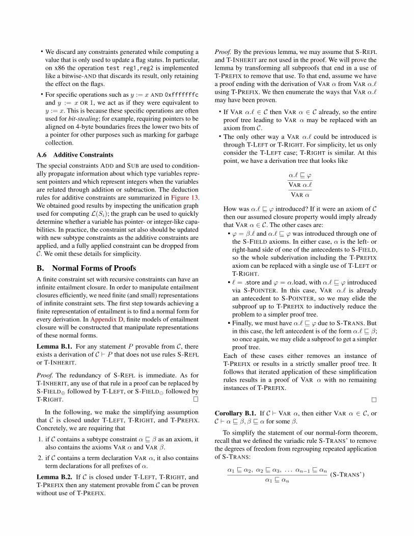
• We discard any constraints generated while computing avalue that is only used to update a flag status. In particular,on x86 the operation test reg1,reg2 is implementedlike a bitwise-AND that discards its result, only retainingthe effect on the flags.

• For specific operations such as y := x AND 0xfffffffcand y := x OR 1, we act as if they were equivalent toy := x. This is because these specific operations are oftenused for bit-stealing; for example, requiring pointers to bealigned on 4-byte boundaries frees the lower two bits ofa pointer for other purposes such as marking for garbagecollection.

A.6 Additive ConstraintsThe special constraints ADD and SUB are used to condition-ally propagate information about which type variables repre-sent pointers and which represent integers when the variablesare related through addition or subtraction. The deductionrules for additive constraints are summarized in Figure 13.We obtained good results by inspecting the unification graphused for computing L(Si); the graph can be used to quicklydetermine whether a variable has pointer- or integer-like capa-bilities. In practice, the constraint set also should be updatedwith new subtype constraints as the additive constraints areapplied, and a fully applied constraint can be dropped fromC. We omit these details for simplicity.

B. Normal Forms of ProofsA finite constraint set with recursive constraints can have aninfinite entailment closure. In order to manipulate entailmentclosures efficiently, we need finite (and small) representationsof infinite constraint sets. The first step towards achieving afinite representation of entailment is to find a normal form forevery derivation. In Appendix D, finite models of entailmentclosure will be constructed that manipulate representationsof these normal forms.

Lemma B.1. For any statement P provable from C, thereexists a derivation of C ` P that does not use rules S-REFLor T-INHERIT.

Proof. The redundancy of S-REFL is immediate. As forT-INHERIT, any use of that rule in a proof can be replaced byS-FIELD⊕ followed by T-LEFT, or S-FIELD followed byT-RIGHT.

In the following, we make the simplifying assumptionthat C is closed under T-LEFT, T-RIGHT, and T-PREFIX.Concretely, we are requiring that

1. if C contains a subtype constraint α v β as an axiom, italso contains the axioms VAR α and VAR β.

2. if C contains a term declaration VAR α, it also containsterm declarations for all prefixes of α.

Lemma B.2. If C is closed under T-LEFT, T-RIGHT, andT-PREFIX then any statement provable from C can be provenwithout use of T-PREFIX.

Proof. By the previous lemma, we may assume that S-REFLand T-INHERIT are not used in the proof. We will prove thelemma by transforming all subproofs that end in a use ofT-PREFIX to remove that use. To that end, assume we havea proof ending with the derivation of VAR α from VAR α.`using T-PREFIX. We then enumerate the ways that VAR α.`may have been proven.

• If VAR α.` ∈ C then VAR α ∈ C already, so the entireproof tree leading to VAR α may be replaced with anaxiom from C.

• The only other way a VAR α.` could be introduced isthrough T-LEFT or T-RIGHT. For simplicity, let us onlyconsider the T-LEFT case; T-RIGHT is similar. At thispoint, we have a derivation tree that looks like

α.` v ϕVAR α.`

VAR α

How was α.` v ϕ introduced? If it were an axiom of Cthen our assumed closure property would imply alreadythat VAR α ∈ C. The other cases are:ϕ = β.` and α.` v ϕ was introduced through one ofthe S-FIELD axioms. In either case, α is the left- orright-hand side of one of the antecedents to S-FIELD,so the whole subderivation including the T-PREFIXaxiom can be replaced with a single use of T-LEFT orT-RIGHT.` = .store and ϕ = α.load, with α.` v ϕ introducedvia S-POINTER. In this case, VAR α.` is alreadyan antecedent to S-POINTER, so we may elide thesubproof up to T-PREFIX to inductively reduce theproblem to a simpler proof tree.Finally, we must have α.` v ϕ due to S-TRANS. Butin this case, the left antecedent is of the form α.` v β;so once again, we may elide a subproof to get a simplerproof tree.

Each of these cases either removes an instance ofT-PREFIX or results in a strictly smaller proof tree. Itfollows that iterated application of these simplificationrules results in a proof of VAR α with no remaininginstances of T-PREFIX.

Corollary B.1. If C ` VAR α, then either VAR α ∈ C, orC ` α v β, β v α for some β.

To simplify the statement of our normal-form theorem,recall that we defined the variadic rule S-TRANS’ to removethe degrees of freedom from regrouping repeated applicationof S-TRANS:

α1 v α2, α2 v α3, . . . αn−1 v αnα1 v αn

(S-TRANS’)

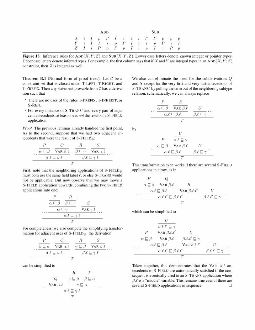
ADD SUB

X i I p P I i i I P P p p pY i I I i p P I i i p P i IZ I i P p P p I i p I i P p

Figure 13. Inference rules for ADD(X,Y ;Z) and SUB(X,Y ;Z). Lower case letters denote known integer or pointer types.Upper case letters denote inferred types. For example, the first column says that ifX and Y are integral types in an ADD(X,Y ;Z)constraint, then Z is integral as well.

Theorem B.1 (Normal form of proof trees). Let C be aconstraint set that is closed under T-LEFT, T-RIGHT, andT-PREFIX. Then any statement provable from C has a deriva-tion such that

• There are no uses of the rules T-PREFIX, T-INHERIT, orS-REFL.

• For every instance of S-TRANS’ and every pair of adja-cent antecedents, at least one is not the result of a S-FIELDapplication.

Proof. The previous lemmas already handled the first point.As to the second, suppose that we had two adjacent an-tecedents that were the result of S-FIELD⊕:

· · ·

P

α v βQ

VAR β.`

α.` v β.`

R

β v γS

VAR γ.`

β.` v γ.` · · ·

T

First, note that the neighboring applications of S-FIELD⊕must both use the same field label `, or else S-TRANS wouldnot be applicable. But now observe that we may move aS-FIELD application upwards, combining the two S-FIELDapplications into one:

· · ·

P

α v βR

β v γα v γ

S

VAR γ.`

α.` v γ.` · · ·

T

For completeness, we also compute the simplifying transfor-mation for adjacent uses of S-FIELD: the derivation

· · ·

P

β v αQ

VAR α.`

α.` v β.`

R

γ v βS

VAR β.`

β.` v γ.` · · ·

T

can be simplified to

· · ·

Q

VAR α.`

R

γ v βP

β v αγ v α

α.` v γ.` · · ·

T

We also can eliminate the need for the subderivations Qand S except for the very first and very last antecedents ofS-TRANS’ by pulling the term out of the neighboring subtyperelation; schematically, we can always replace

· · ·

P

α v βS

VAR β.`

α.` v β.`U

β.` v γ · · ·

T

by

· · ·

P

α v β

U

β.` v γVAR β.`

α.` v β.`U

β.` v γ · · ·

T

This transformation even works if there are several S-FIELDapplications in a row, as in

· · ·

P

α v βQ

VAR β.`

α.` v β.`R

VAR β.`.`′

α.`.`′ v β.`.`′U

β.`.`′ v γ · · ·

T

which can be simplified to

· · ·

P

α v β

U

β.`.`′ v γVAR β.`.`′

VAR β.`

α.` v β.`

U

β.`.`′ v γVAR β.`.`′

α.`.`′ v β.`.`′U

β.`.`′ v γ · · ·

T

Taken together, this demonstrates that the VAR β.` an-tecedents to S-FIELD are automatically satisfied if the con-sequent is eventually used in an S-TRANS application whereβ.` is a “middle” variable. This remains true even if there areseveral S-FIELD applications in sequence.

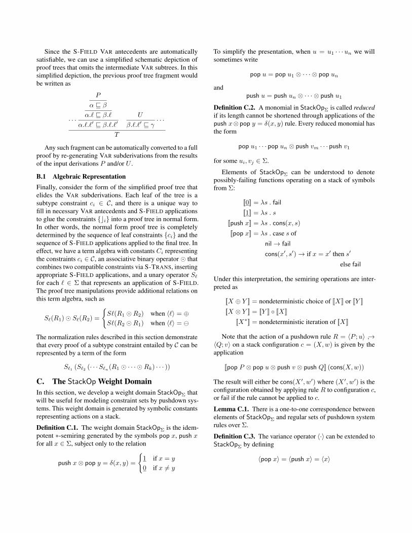
Since the S-FIELD VAR antecedents are automaticallysatisfiable, we can use a simplified schematic depiction ofproof trees that omits the intermediate VAR subtrees. In thissimplified depiction, the previous proof tree fragment wouldbe written as

· · ·

P

α v βα.` v β.`

α.`.`′ v β.`.`′U

β.`.`′ v γ · · ·

T

Any such fragment can be automatically converted to a fullproof by re-generating VAR subderivations from the resultsof the input derivations P and/or U .

B.1 Algebraic RepresentationFinally, consider the form of the simplified proof tree thatelides the VAR subderivations. Each leaf of the tree is asubtype constraint ci ∈ C, and there is a unique way tofill in necessary VAR antecedents and S-FIELD applicationsto glue the constraints {ci} into a proof tree in normal form.In other words, the normal form proof tree is completelydetermined by the sequence of leaf constraints {ci} and thesequence of S-FIELD applications applied to the final tree. Ineffect, we have a term algebra with constants Ci representingthe constraints ci ∈ C, an associative binary operator � thatcombines two compatible constraints via S-TRANS, insertingappropriate S-FIELD applications, and a unary operator S`for each ` ∈ Σ that represents an application of S-FIELD.The proof tree manipulations provide additional relations onthis term algebra, such as

S`(R1)� S`(R2) =

{S`(R1 �R2) when 〈`〉 = ⊕S`(R2 �R1) when 〈`〉 =

The normalization rules described in this section demonstratethat every proof of a subtype constraint entailed by C can berepresented by a term of the form

S`1 (S`2 (· · ·S`n(R1 � · · · �Rk) · · · ))

C. The StackOp Weight DomainIn this section, we develop a weight domain StackOpΣ thatwill be useful for modeling constraint sets by pushdown sys-tems. This weight domain is generated by symbolic constantsrepresenting actions on a stack.

Definition C.1. The weight domain StackOpΣ is the idem-potent ∗-semiring generated by the symbols pop x, push xfor all x ∈ Σ, subject only to the relation

push x⊗ pop y = δ(x, y) =

{1 if x = y

0 if x 6= y

To simplify the presentation, when u = u1 · · ·un we willsometimes write

pop u = pop u1 ⊗ · · · ⊗ pop un

andpush u = push un ⊗ · · · ⊗ push u1

Definition C.2. A monomial in StackOpΣ is called reducedif its length cannot be shortened through applications of thepush x⊗pop y = δ(x, y) rule. Every reduced monomial hasthe form

pop u1 · · · pop un ⊗ push vm · · · push v1

for some ui, vj ∈ Σ.

Elements of StackOpΣ can be understood to denotepossibly-failing functions operating on a stack of symbolsfrom Σ:

[[0]] = λs . fail

[[1]] = λs . s

[[push x]] = λs . cons(x, s)

[[pop x]] = λs . case s of

nil→ fail

cons(x′, s′)→ if x = x′ then s′

else fail

Under this interpretation, the semiring operations are inter-preted as

[[X ⊕ Y ]] = nondeterministic choice of [[X]] or [[Y ]]

[[X ⊗ Y ]] = [[Y ]] ◦ [[X]]

[[X∗]] = nondeterministic iteration of [[X]]

Note that the action of a pushdown rule R = 〈P ;u〉 ↪→〈Q; v〉 on a stack configuration c = (X,w) is given by theapplication

[[pop P ⊗ pop u⊗ push v ⊗ push Q]] (cons(X,w))

The result will either be cons(X ′, w′) where (X ′, w′) is theconfiguration obtained by applying rule R to configuration c,or fail if the rule cannot be applied to c.

Lemma C.1. There is a one-to-one correspondence betweenelements of StackOpΣ and regular sets of pushdown systemrules over Σ.

Definition C.3. The variance operator 〈·〉 can be extended toStackOpΣ by defining

〈pop x〉 = 〈push x〉 = 〈x〉

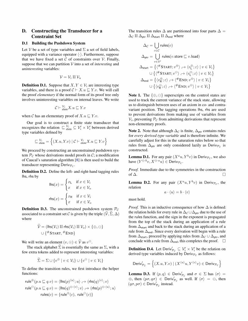
D. Constructing the Transducer for aConstraint Set

D.1 Building the Pushdown SystemLet V be a set of type variables and Σ a set of field labels,equipped with a variance operator 〈·〉. Furthermore, supposethat we have fixed a set C of constraints over V . Finally,suppose that we can partition V into a set of interesting anduninteresting variables:

V = Vi q VuDefinition D.1. Suppose that X,Y ∈ Vi are interesting typevariables, and there is a proof C ` X.u v Y.v. We will callthe proof elementary if the normal form of its proof tree onlyinvolves uninteresting variables on internal leaves. We write

C ` VielemX.u v Y.v

when C has an elementary proof of X.u v Y.v.

Our goal is to construct a finite state transducer thatrecognizes the relation v Vielem ⊆ V ′i × V ′i between derivedtype variables defined by

v Vielem ={

(X.u, Y.v) | C ` VielemX.u v Y.v}

We proceed by constructing an unconstrained pushdown sys-tem PC whose derivations model proofs in C; a modificationof Caucal’s saturation algorithm [8] is then used to build thetransducer representing DerivPC .

Definition D.2. Define the left- and right-hand tagging ruleslhs, rhs by

lhs(x) =

{xL if x ∈ Vix if x ∈ Vo

rhs(x) =

{xR if x ∈ Vix if x ∈ Vo

Definition D.3. The unconstrained pushdown system PCassociated to a constraint set C is given by the triple (V, Σ,∆)where

V = (lhs(Vi)q rhs(Vi)q Vo)× {⊕,}∪ {#START,#END}

We will write an element (v,�) ∈ V as v�.The stack alphabet Σ is essentially the same as Σ, with a

few extra tokens added to represent interesting variables:

Σ = Σ ∪ {v⊕ | v ∈ Vi} ∪ {v | v ∈ Vi}

To define the transition rules, we first introduce the helperfunctions:

rule⊕(p.u v q.v) = 〈lhs(p)〈u〉;u〉 ↪→ 〈rhs(q)〈v〉; v〉rule(p.u v q.v) = 〈lhs(q)·〈v〉; v〉 ↪→ 〈rhs(p)·〈u〉;u〉

rules(c) = {rule⊕(c), rule(c)}

The transition rules ∆ are partitioned into four parts ∆ =∆C q∆ptr q∆start q∆end where

∆C =⋃c∈C

rules(c)

∆ptr =⋃v∈V′

rules(v.store v v.load)

∆start ={〈#START; v⊕〉 ↪→ 〈v⊕L ; ε〉 | v ∈ Vi

}∪{〈#START; v〉 ↪→ 〈vL ; ε〉 | v ∈ Vi

}∆end =

{〈v⊕R ; ε〉 ↪→ 〈#END; v⊕〉 | v ∈ Vi

}∪{〈vR ; ε〉 ↪→ 〈#END; v〉 | v ∈ Vi

}Note 1. The {⊕,} superscripts on the control states areused to track the current variance of the stack state, allowingus to distinguish between uses of an axiom in co- and contra-variant position. The tagging operations lhs, rhs are usedto prevent derivations from making use of variables fromVi, preventing PC from admitting derivations that representnon-elementary proofs.

Note 2. Note that although ∆C is finite, ∆ptr contains rulesfor every derived type variable and is therefore infinite. Wecarefully adjust for this in the saturation rules below so thatrules from ∆ptr are only considered lazily as DerivPC isconstructed.

Lemma D.1. For any pair (Xau, Y bv) in DerivPC , we alsohave (Y ·bv,X·au) ∈ DerivPC .

Proof. Immediate due to the symmetries in the constructionof ∆.

Lemma D.2. For any pair (Xau, Y bv) in DerivPC , therelation

a · 〈u〉 = b · 〈v〉must hold.

Proof. This is an inductive consequence of how ∆ is defined:the relation holds for every rule in ∆C∪∆ptr due to the use ofthe rules function, and the sign in the exponent is propagatedfrom the top of the stack during an application of a rulefrom ∆start and back to the stack during an application of arule from ∆end. Since every derivation will begin with a rulefrom ∆start, proceed by applying rules from ∆C ∪∆ptr, andconclude with a rule from ∆end, this completes the proof.

Definition D.4. Let Deriv′PC ⊆ V ′i × V ′i be the relation onderived type variables induced by DerivPC as follows:

Deriv′PC ={

(X.u, Y.v) | (X〈u〉u, Y 〈v〉v) ∈ DerivPC}

Lemma D.3. If (p, q) ∈ Deriv′PC and σ ∈ Σ has 〈σ〉 =⊕, then (pσ, qσ) ∈ Deriv′PC as well. If 〈σ〉 = , then(qσ, pσ) ∈ Deriv′PC instead.

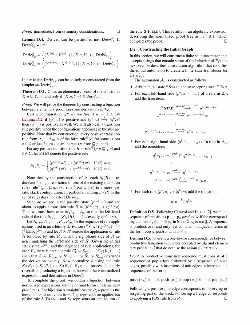
Proof. Immediate, from symmetry considerations.

Lemma D.4. DerivPC can be partitioned into Deriv⊕PC qDerivPC where

Deriv⊕PC ={

(X〈u〉u, Y 〈v〉v) | (X.u, Y.v) ∈ Deriv′PC

}DerivPC =

{(Y ·〈v〉v,X·〈u〉u) | (X.u, Y.v) ∈ Deriv′PC

}

In particular, DerivPC can be entirely reconstructed from thesimpler set Deriv′PC .

Theorem D.1. C has an elementary proof of the constraintX.u v Y.v if and only if (X.u, Y.v) ∈ Deriv′PC .

Proof. We will prove the theorem by constructing a bijectionbetween elementary proof trees and derivations in PC .

Call a configuration (pa, u) positive if a = 〈u〉. ByLemma D.2, if (pa, u) is positive and (pa, u)

∗−→ (qb, v)then (qb, v) is positive as well. We will also call a transitionrule positive when the configurations appearing in the rule arepositive. Note that by construction, every positive transitionrule from ∆C ∪∆ptr is of the form rule⊕(c) for some axiomc ∈ C or load/store constraint c = (p.store v p.load).

For any positive transition ruleR = rule⊕(p.u v q.v) and` ∈ Σ, let S`(R) denote the positive rule

S`(R) =

{〈p〈u`〉;u`〉 ↪→ 〈q〈v`〉; v`〉 if 〈`〉 = ⊕〈q〈v`〉; v`〉 ↪→ 〈p〈u`〉;u`〉 if 〈`〉 =

Note that by the construction of ∆, each S`(R) is re-dundant, being a restriction of one of the existing transitionrules rule⊕(p.u v q.v) or rule(p.u v q.v) to a more spe-cific stack configuration. In particular, adding S`(R) to theset of rules does not affect DerivPC .

Suppose we are in the positive state (p〈w〉, w) and areabout to apply a transition rule R = 〈p〈u〉;u〉 ↪→ 〈q〈v〉; v〉.Then we must have w = u`1`2 · · · `n, so that the left-handside of the rule S`n(· · · (S`1(R)) · · · ) is exactly 〈p〈w〉;w〉.

LetRstart, R1, · · · , Rn, Rend be the sequence of rule appli-cations used in an arbitrary derivation (#START, p〈u〉u)

∗−→(#END, q〈v〉v) and let R�R′ denote the application of ruleR followed by rule R′, with the right-hand side of R ex-actly matching the left-hand side of R′. Given the initialstack state p〈u〉u and the sequence of rule applications, foreach Rk there is a unique rule R′k = S`kn(· · · (S`k1 (Rk)) · · · )such that ∂ = R′start � R′1 � · · · � R′n � R′end describesthe derivation exactly. Now normalize ∂ using the ruleS`(Ri) � S`(Rj) 7→ S`(Ri � Rj); this process is clearlyreversible, producing a bijection between these normalizedexpressions and derivations in Deriv⊕PC .

To complete the proof, we obtain a bijection betweennormalized expressions and the normal forms of elementaryproof trees. The bijection is straightforward:Ri represents theintroduction of an axiom from C, � represents an applicationof the rule S-TRANS, and S` represents an application of

the rule S-FIELD`. This results in an algebraic expressiondescribing the normalized proof tree as in § B.1, whichcompletes the proof.

D.2 Constructing the Initial GraphIn this section, we will construct a finite state automaton thataccepts strings that encode some of the behavior of PC; thenext section describes a saturation algorithm that modifiesthe initial automaton to create a finite state transducer forDeriv′PC .

The automaton AC is constructed as follows:

1. Add an initial state #START and an accepting state #END.

2. For each left-hand side 〈pa;u1 · · ·un〉 of a rule in ∆C ,add the transitions

#STARTpop pa·〈u1...un〉−→ pa·〈u1...un〉

pa·〈u1...un〉 pop u1−→ pa·〈u2...un〉u1

...

pa·〈un〉u1 . . . un−1pop un−→ pau1 . . . un

3. For each right-hand side 〈qb; v1 · · · vn〉 of a rule in ∆C ,add the transitions

qbv1 . . . vnpush vn−→ qb·〈vn〉v1 . . . vn−1

...

qb·〈v2...vn〉v1push v1−→ qb·〈v1...vn〉

qb·〈v1...vn〉push qb·〈v1...vn〉−→ #END

4. For each rule 〈pa;u〉 ↪→ 〈qb; v〉, add the transition

pau1−→ qbv

Definition D.5. Following Carayol and Hague [7], we call asequence of transitions p1 · · · pn productive if the correspond-ing element p1 ⊗ · · · ⊗ pn in StackOpΣ is not 0. A sequenceis productive if and only if it contains no adjacent terms ofthe form pop y, push x with x 6= y.

Lemma D.5. There is a one-to-one correspondence betweenproductive transition sequences accepted by AC and elemen-tary proofs in C that do not use the axiom S-POINTER.

Proof. A productive transition sequence must consist of asequence of pop edges followed by a sequence of pushedges, possibly with insertions of unit edges or intermediatesequences of the form

push (un)⊗ · · · ⊗ push (u1)⊗ pop (u1)⊗ · · · ⊗ pop (un)

Following a push or pop edge corresponds to observing orforgetting part of the stack. Following a 1 edge correspondsto applying a PDS rule from PC .

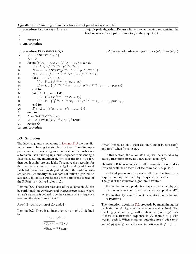
Algorithm D.1 Converting a transducer from a set of pushdown system rules1: procedure ALLPATHS(V,E, x, y) . Tarjan’s path algorithm. Return a finite state automaton recognizing the

label sequence for all paths from x to y in the graph (V,E).2: . . .3: return Q4: end procedure

5: procedure TRANSDUCER(∆C) .∆C is a set of pushdown system rules 〈pa;u〉 ↪→ 〈qb; v〉6: V ← {#START,#END}7: E ← ∅8: for all 〈pa;u1 · · ·un〉 ↪→ 〈qb; v1 · · · vm〉 ∈ ∆C do9: V ← V ∪ {pa·〈u1···un〉, qb·〈v1···vm〉}

10: E ← E ∪ {(#START, pa·〈u1···un〉, pop pa·〈u1···un〉)}11: E ← E ∪ {(qb·〈v1···vm〉,#END, push qb·〈v1···vm〉)}12: for i← 1 . . . n− 1 do13: V ← V ∪ {pa·〈ui+1···un〉u1 . . . ui}14: E ← E ∪ {(pa·〈ui···un〉u1 . . . ui−1, p

a·〈ui+1···un〉u1 . . . ui, pop ui)}15: end for16: for j ← 1 . . .m− 1 do17: V ← V ∪ {qb·〈vj+1···um〉v1 . . . vj}18: E ← E ∪ {(qb·〈vj+1···vm〉v1 . . . vj , q

b·〈vj ···vm〉v1 . . . vj−1, push vj)}19: end for20: E ← E ∪ {(pau1 . . . un, q

bv1 . . . vm, 1)}21: end for22: E ← SATURATED(V,E)23: Q← ALLPATHS(V,E,#START,#END)24: return Q25: end procedure

D.3 SaturationThe label sequences appearing in Lemma D.5 are tantaliz-ingly close to having the simple structure of building up apop sequence representing an initial state of the pushdownautomaton, then building up a push sequence representing afinal state. But the intermediate terms of the form “push u,then pop it again” are unwieldy. To remove the necessity forthose sequences, we can saturate AC by adding additional1-labeled transitions providing shortcuts to the push/pop sub-sequences. We modify the standard saturation algorithm toalso lazily instantiate transitions which correspond to uses ofthe S-POINTER-derived rules in ∆ptr.

Lemma D.6. The reachable states of the automaton AC canbe partitioned into covariant and contravariant states, wherea state’s variance is defined to be the variance of any sequencereaching the state from #START.

Proof. By construction of ∆C and AC .

Lemma D.7. There is an involution n 7→ n on AC definedby

xau = x·au#START = #END

#END = #START

Proof. Immediate due to the use of the rule constructors rule⊕

and rule when forming ∆C .

In this section, the automaton AC will be saturated byadding transitions to create a new automaton Asat

C .

Definition D.6. A sequence is called reduced if it is produc-tive and contains no factors of the form pop x⊗ push x.

Reduced productive sequences all have the form of asequence of pops, followed by a sequence of pushes.The goal of the saturation algorithm is twofold:

1. Ensure that for any productive sequence accepted by ACthere is an equivalent reduced sequence accepted by Asat

C .

2. Ensure that AsatC can represent elementary proofs that use

S-POINTER.

The saturation algorithm D.2 proceeds by maintaining, foreach state q ∈ AC , a set of reaching-pushes R(q). Thereaching push set R(q) will contain the pair (`, p) onlyif there is a transition sequence in AC from p to q withweight push `. When q has an outgoing pop ` edge to q′

and (`, p) ∈ R(q), we add a new transition p1→ q′ to AC .

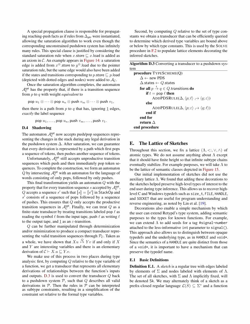
A special propagation clause is responsible for propagat-ing reaching-push facts as if rules from ∆ptr were instantiated,allowing the saturation algorithm to work even though thecorresponding unconstrained pushdown system has infinitelymany rules. This special clause is justified by considering thestandard saturation rule when x.store v x.load is added asan axiom in C. An example appears in Figure 14: a saturationedge is added from x⊕.store to y⊕.load due to the pointersaturation rule, but the same edge would also have been addedif the states and transitions corresponding to p.store v p.load(depicted with dotted edges and nodes) were added to AC .

Once the saturation algorithm completes, the automatonAsatC has the property that, if there is a transition sequence

from p to q with weight equivalent to

pop u1 ⊗ · · · ⊗ pop un ⊗ push vm ⊗ · · · ⊗ push v1,

then there is a path from p to q that has, ignoring 1 edges,exactly the label sequence

pop u1, . . . , pop un, push vm, . . . , push v1.

D.4 ShadowingThe automaton Asat

C now accepts push/pop sequences repre-senting the changes in the stack during any legal derivation inthe pushdown system ∆. After saturation, we can guaranteethat every derivation is represented by a path which first popsa sequence of tokens, then pushes another sequence of tokens.

Unfortunately, AsatC still accepts unproductive transition

sequences which push and then immediately pop token se-quences. To complete the construction, we form an automatonQ by intersectingAsat

C with an automaton for the language ofwords consisting of only pops, followed by only pushes.

This final transformation yields an automaton Q with theproperty that for every transition sequence s accepted byAsat

C ,Q accepts a sequence s′ such that [[s]] = [[s′]] in StackOp ands′ consists of a sequence of pops followed by a sequenceof pushes. This ensures that Q only accepts the productivetransition sequences in Asat

C . Finally, we can treat Q as afinite-state transducer by treating transitions labeled pop ` asreading the symbol ` from the input tape, push ` as writing `to the output tape, and 1 as an ε-transition.Q can be further manipulated through determinization

and/or minimization to produce a compact transducer repre-senting the valid transition sequences through PC . Taken asa whole, we have shown that Xu

Q7→ Y v if and only if Xand Y are interesting variables and there is an elementaryderivation of C ` X.u v Y.v.

We make use of this process in two places during typeanalysis: first, by computing Q relative to the type variable ofa function, we get a transducer that represents all elementaryderivations of relationships between the function’s inputsand outputs. D.3 is used to convert the transducer Q backto a pushdown system P , such that Q describes all validderivations in P . Then the rules in P can be interpretedas subtype constraints, resulting in a simplification of theconstraint set relative to the formal type variables.

Second, by computing Q relative to the set of type con-stants we obtain a transducer that can be efficiently queriedto determine which derived type variables are bound aboveor below by which type constants. This is used by the SOLVEprocedure in F.2 to populate lattice elements decorating theinferred sketches.

Algorithm D.3 Converting a transducer to a pushdown sys-tem

procedure TYPESCHEME(Q)∆← new PDS∆.states← Q.states

for all p t→ q ∈ Q.transitions doif t = pop ` then

ADDPDSRULE(∆, 〈p; `〉 ↪→ 〈q; ε〉)else

ADDPDSRULE(∆, 〈p; ε〉 ↪→ 〈q; `〉)end if

end forreturn ∆

end procedure

E. The Lattice of SketchesThroughout this section, we fix a lattice (Λ, <:,∨,∧) ofatomic types. We do not assume anything about Λ exceptthat it should have finite height so that infinite subtype chainseventually stabilize. For example purposes, we will take Λ tobe the lattice of semantic classes depicted in Figure 15.

Our initial implementation of sketches did not use theauxiliary lattice Λ. We found that adding these decorations tothe sketches helped preserve high-level types of interest to theend user during type inference. This allows us to recover high-level C and Windows typedefs such as size_t, FILE, HANDLE,and SOCKET that are useful for program understanding andreverse engineering, as noted by Lin et al. [19].

Decorations also enable a simple mechanism by whichthe user can extend Retypd’s type system, adding semanticpurposes to the types for known functions. For example,we can extend Λ to add seeds for a tag #signal-numberattached to the less-informative int parameter to signal().This approach also allows us to distinguish between opaquetypedefs and the underlying type, as in HANDLE and void*.Since the semantics of a HANDLE are quite distinct from thoseof a void*, it is important to have a mechanism that canpreserve the typedef name.

E.1 Basic DefinitionsDefinition E.1. A sketch is a regular tree with edges labeledby elements of Σ and nodes labeled with elements of Λ.The set of all sketches, with Σ and Λ implicitly fixed, willbe denoted Sk. We may alternately think of a sketch as aprefix-closed regular language L(S) ⊆ Σ∗ and a function

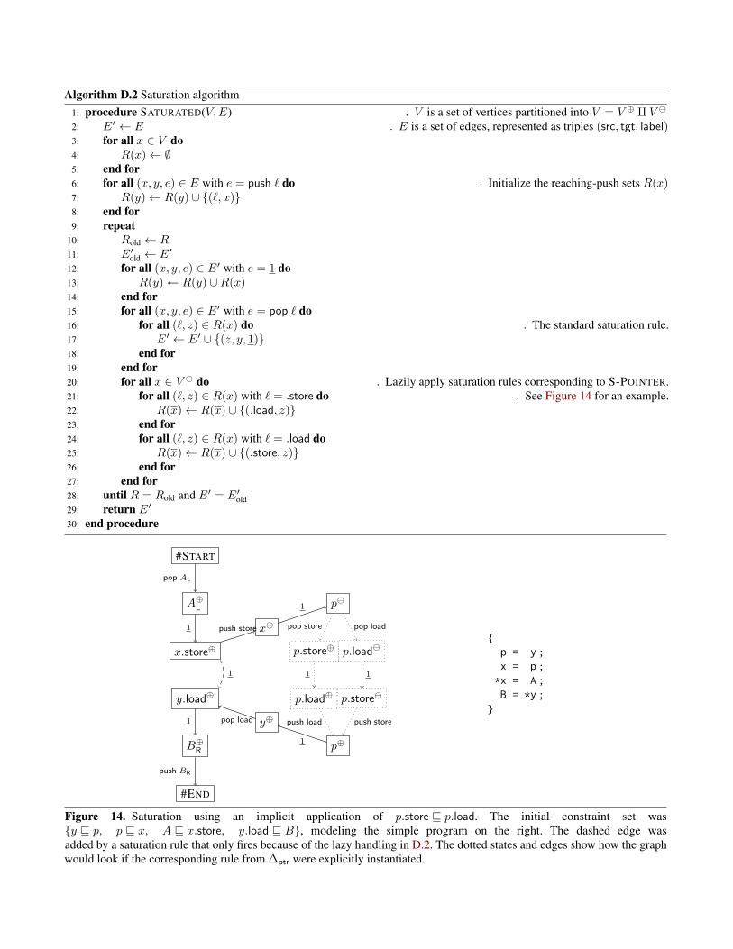
Algorithm D.2 Saturation algorithm1: procedure SATURATED(V,E) . V is a set of vertices partitioned into V = V ⊕ q V 2: E′ ← E . E is a set of edges, represented as triples (src, tgt, label)3: for all x ∈ V do4: R(x)← ∅5: end for6: for all (x, y, e) ∈ E with e = push ` do . Initialize the reaching-push sets R(x)7: R(y)← R(y) ∪ {(`, x)}8: end for9: repeat

10: Rold ← R11: E′old ← E′

12: for all (x, y, e) ∈ E′ with e = 1 do13: R(y)← R(y) ∪R(x)14: end for15: for all (x, y, e) ∈ E′ with e = pop ` do16: for all (`, z) ∈ R(x) do . The standard saturation rule.17: E′ ← E′ ∪ {(z, y, 1)}18: end for19: end for20: for all x ∈ V do . Lazily apply saturation rules corresponding to S-POINTER.21: for all (`, z) ∈ R(x) with ` = .store do . See Figure 14 for an example.22: R(x)← R(x) ∪ {(.load, z)}23: end for24: for all (`, z) ∈ R(x) with ` = .load do25: R(x)← R(x) ∪ {(.store, z)}26: end for27: end for28: until R = Rold and E′ = E′old29: return E′30: end procedure

#START

A⊕L

x.store⊕

x

p

p.store⊕ p.load

p.load⊕ p.store

p⊕

y⊕

y.load⊕

B⊕R

#END

pop AL

1

1

push BR

push store

pop load

1

1

pop store pop load

1 1

push load push store

1

{p = y;x = p;*x = A;B = *y;

}

Figure 14. Saturation using an implicit application of p.store v p.load. The initial constraint set was{y v p, p v x, A v x.store, y.load v B}, modeling the simple program on the right. The dashed edge wasadded by a saturation rule that only fires because of the lazy handling in D.2. The dotted states and edges show how the graphwould look if the corresponding rule from ∆ptr were explicitly instantiated.

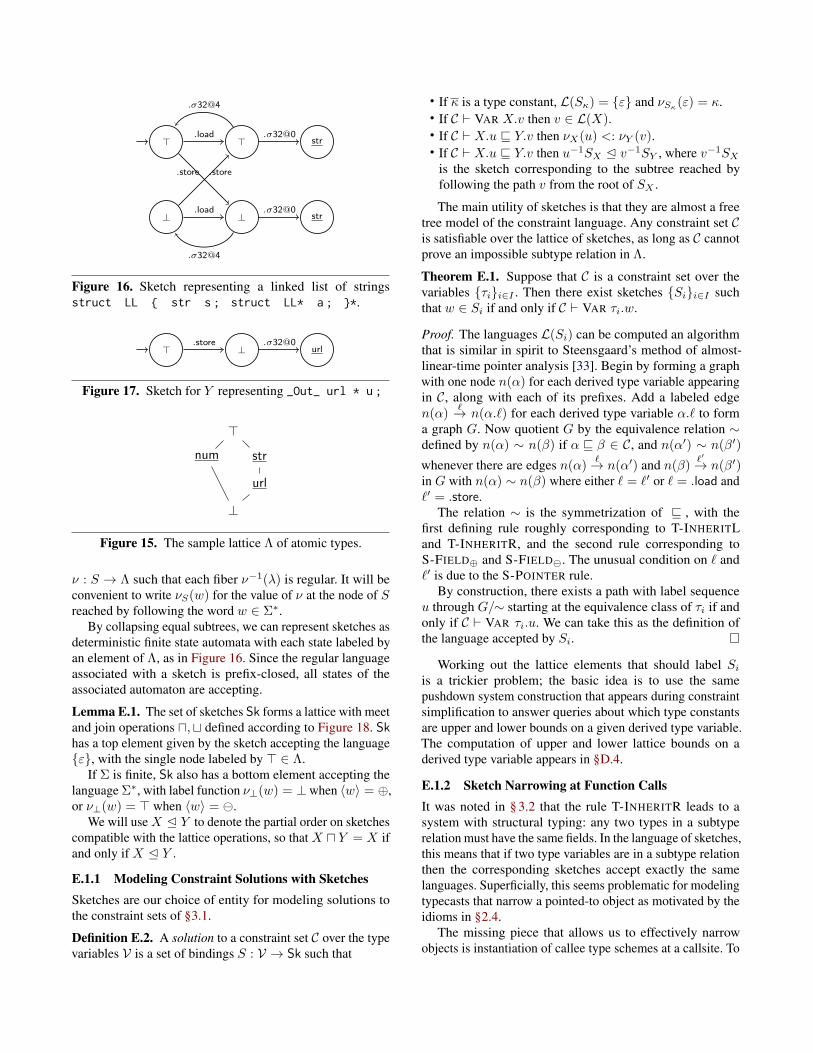
> > str

⊥ ⊥ str

.store.store

.σ32@0

.σ32@0

.load

.load

.σ32@4

.σ32@4

Figure 16. Sketch representing a linked list of stringsstruct LL { str s; struct LL* a; }*.

> ⊥ url.σ32@0.store

Figure 17. Sketch for Y representing _Out_ url * u;

>num str

url

⊥

Figure 15. The sample lattice Λ of atomic types.

ν : S → Λ such that each fiber ν−1(λ) is regular. It will beconvenient to write νS(w) for the value of ν at the node of Sreached by following the word w ∈ Σ∗.

By collapsing equal subtrees, we can represent sketches asdeterministic finite state automata with each state labeled byan element of Λ, as in Figure 16. Since the regular languageassociated with a sketch is prefix-closed, all states of theassociated automaton are accepting.

Lemma E.1. The set of sketches Sk forms a lattice with meetand join operations u,t defined according to Figure 18. Skhas a top element given by the sketch accepting the language{ε}, with the single node labeled by > ∈ Λ.

If Σ is finite, Sk also has a bottom element accepting thelanguage Σ∗, with label function ν⊥(w) = ⊥when 〈w〉 = ⊕,or ν⊥(w) = > when 〈w〉 = .

We will useX E Y to denote the partial order on sketchescompatible with the lattice operations, so that X u Y = X ifand only if X E Y .

E.1.1 Modeling Constraint Solutions with SketchesSketches are our choice of entity for modeling solutions tothe constraint sets of §3.1.

Definition E.2. A solution to a constraint set C over the typevariables V is a set of bindings S : V → Sk such that

• If κ is a type constant, L(Sκ) = {ε} and νSκ(ε) = κ.• If C ` VAR X.v then v ∈ L(X).• If C ` X.u v Y.v then νX(u) <: νY (v).• If C ` X.u v Y.v then u−1SX E v−1SY , where v−1SX

is the sketch corresponding to the subtree reached byfollowing the path v from the root of SX .

The main utility of sketches is that they are almost a freetree model of the constraint language. Any constraint set Cis satisfiable over the lattice of sketches, as long as C cannotprove an impossible subtype relation in Λ.

Theorem E.1. Suppose that C is a constraint set over thevariables {τi}i∈I . Then there exist sketches {Si}i∈I suchthat w ∈ Si if and only if C ` VAR τi.w.

Proof. The languages L(Si) can be computed an algorithmthat is similar in spirit to Steensgaard’s method of almost-linear-time pointer analysis [33]. Begin by forming a graphwith one node n(α) for each derived type variable appearingin C, along with each of its prefixes. Add a labeled edgen(α)

`→ n(α.`) for each derived type variable α.` to forma graph G. Now quotient G by the equivalence relation ∼defined by n(α) ∼ n(β) if α v β ∈ C, and n(α′) ∼ n(β′)

whenever there are edges n(α)`→ n(α′) and n(β)

`′→ n(β′)in G with n(α) ∼ n(β) where either ` = `′ or ` = .load and`′ = .store.

The relation ∼ is the symmetrization of v , with thefirst defining rule roughly corresponding to T-INHERITLand T-INHERITR, and the second rule corresponding toS-FIELD⊕ and S-FIELD. The unusual condition on ` and`′ is due to the S-POINTER rule.

By construction, there exists a path with label sequenceu through G/∼ starting at the equivalence class of τi if andonly if C ` VAR τi.u. We can take this as the definition ofthe language accepted by Si.

Working out the lattice elements that should label Siis a trickier problem; the basic idea is to use the samepushdown system construction that appears during constraintsimplification to answer queries about which type constantsare upper and lower bounds on a given derived type variable.The computation of upper and lower lattice bounds on aderived type variable appears in §D.4.

E.1.2 Sketch Narrowing at Function CallsIt was noted in §3.2 that the rule T-INHERITR leads to asystem with structural typing: any two types in a subtyperelation must have the same fields. In the language of sketches,this means that if two type variables are in a subtype relationthen the corresponding sketches accept exactly the samelanguages. Superficially, this seems problematic for modelingtypecasts that narrow a pointed-to object as motivated by theidioms in §2.4.

The missing piece that allows us to effectively narrowobjects is instantiation of callee type schemes at a callsite. To

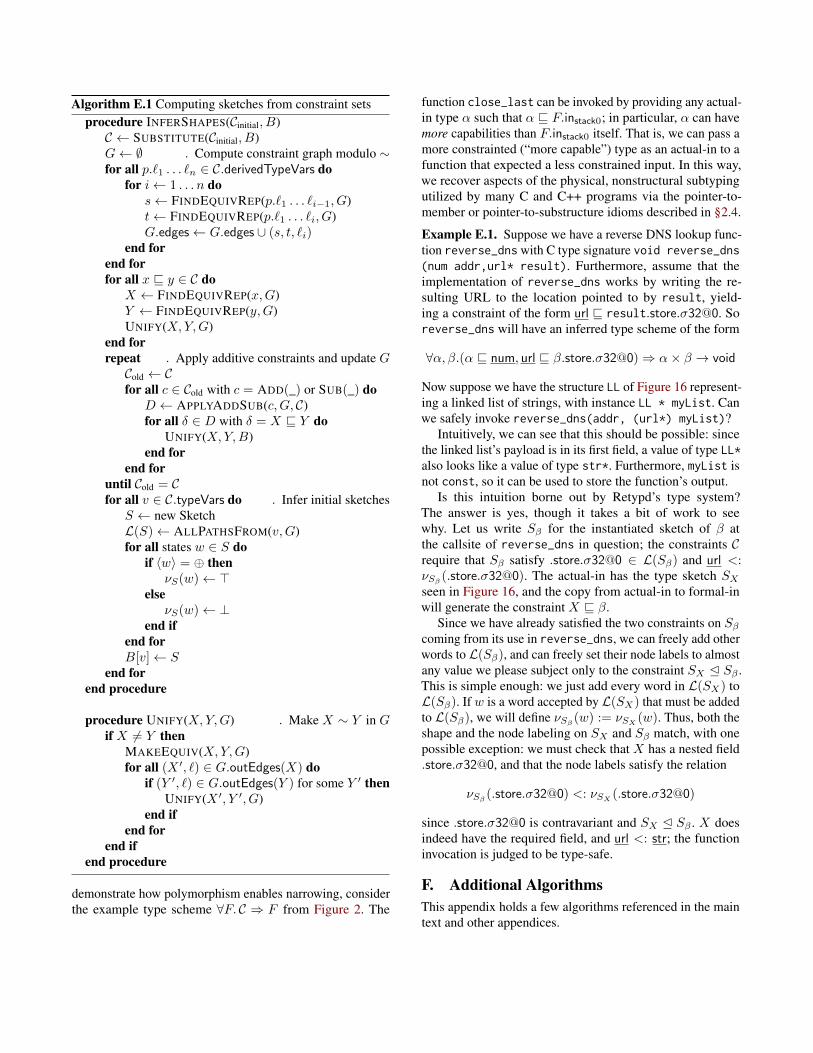
Algorithm E.1 Computing sketches from constraint setsprocedure INFERSHAPES(Cinitial, B)C ← SUBSTITUTE(Cinitial, B)G← ∅ . Compute constraint graph modulo ∼for all p.`1 . . . `n ∈ C.derivedTypeVars do

for i← 1 . . . n dos← FINDEQUIVREP(p.`1 . . . `i−1, G)t← FINDEQUIVREP(p.`1 . . . `i, G)G.edges← G.edges ∪ (s, t, `i)

end forend forfor all x v y ∈ C do

X ← FINDEQUIVREP(x,G)Y ← FINDEQUIVREP(y,G)UNIFY(X,Y,G)

end forrepeat . Apply additive constraints and update GCold ← Cfor all c ∈ Cold with c = ADD(_) or SUB(_) do

D ← APPLYADDSUB(c,G, C)for all δ ∈ D with δ = X v Y do

UNIFY(X,Y,B)end for

end foruntil Cold = Cfor all v ∈ C.typeVars do . Infer initial sketches

S ← new SketchL(S)← ALLPATHSFROM(v,G)for all states w ∈ S do

if 〈w〉 = ⊕ thenνS(w)← >

elseνS(w)← ⊥

end ifend forB[v]← S

end forend procedure

procedure UNIFY(X,Y,G) . Make X ∼ Y in Gif X 6= Y then

MAKEEQUIV(X,Y,G)for all (X ′, `) ∈ G.outEdges(X) do

if (Y ′, `) ∈ G.outEdges(Y ) for some Y ′ thenUNIFY(X ′, Y ′, G)

end ifend for

end ifend procedure

demonstrate how polymorphism enables narrowing, considerthe example type scheme ∀F. C ⇒ F from Figure 2. The

function close_last can be invoked by providing any actual-in type α such that α v F.instack0; in particular, α can havemore capabilities than F.instack0 itself. That is, we can pass amore constrainted (“more capable”) type as an actual-in to afunction that expected a less constrained input. In this way,we recover aspects of the physical, nonstructural subtypingutilized by many C and C++ programs via the pointer-to-member or pointer-to-substructure idioms described in §2.4.

Example E.1. Suppose we have a reverse DNS lookup func-tion reverse_dns with C type signature void reverse_dns(num addr,url* result). Furthermore, assume that theimplementation of reverse_dns works by writing the re-sulting URL to the location pointed to by result, yield-ing a constraint of the form url v result.store.σ32@0. Soreverse_dns will have an inferred type scheme of the form

∀α, β.(α v num, url v β.store.σ32@0)⇒ α× β → void

Now suppose we have the structure LL of Figure 16 represent-ing a linked list of strings, with instance LL * myList. Canwe safely invoke reverse_dns(addr, (url*) myList)?

Intuitively, we can see that this should be possible: sincethe linked list’s payload is in its first field, a value of type LL*also looks like a value of type str*. Furthermore, myList isnot const, so it can be used to store the function’s output.

Is this intuition borne out by Retypd’s type system?The answer is yes, though it takes a bit of work to seewhy. Let us write Sβ for the instantiated sketch of β atthe callsite of reverse_dns in question; the constraints Crequire that Sβ satisfy .store.σ32@0 ∈ L(Sβ) and url <:νSβ (.store.σ32@0). The actual-in has the type sketch SXseen in Figure 16, and the copy from actual-in to formal-inwill generate the constraint X v β.

Since we have already satisfied the two constraints on Sβcoming from its use in reverse_dns, we can freely add otherwords to L(Sβ), and can freely set their node labels to almostany value we please subject only to the constraint SX E Sβ .This is simple enough: we just add every word in L(SX) toL(Sβ). If w is a word accepted by L(SX) that must be addedto L(Sβ), we will define νSβ (w) := νSX (w). Thus, both theshape and the node labeling on SX and Sβ match, with onepossible exception: we must check that X has a nested field.store.σ32@0, and that the node labels satisfy the relation

νSβ (.store.σ32@0) <: νSX (.store.σ32@0)

since .store.σ32@0 is contravariant and SX E Sβ . X doesindeed have the required field, and url <: str; the functioninvocation is judged to be type-safe.

F. Additional AlgorithmsThis appendix holds a few algorithms referenced in the maintext and other appendices.

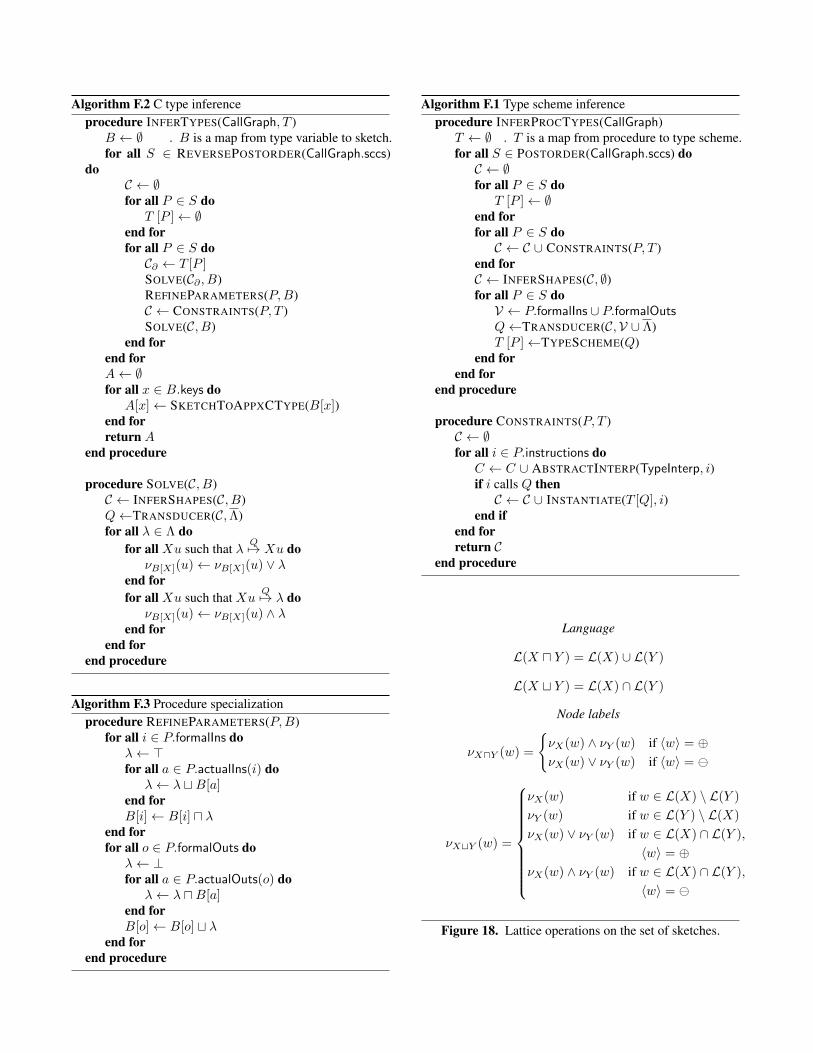
Algorithm F.2 C type inferenceprocedure INFERTYPES(CallGraph, T )

B ← ∅ . B is a map from type variable to sketch.for all S ∈ REVERSEPOSTORDER(CallGraph.sccs)

doC ← ∅for all P ∈ S do

T [P ]← ∅end forfor all P ∈ S doC∂ ← T [P ]SOLVE(C∂ , B)REFINEPARAMETERS(P,B)C ← CONSTRAINTS(P, T )SOLVE(C, B)

end forend forA← ∅for all x ∈ B.keys do

A[x]← SKETCHTOAPPXCTYPE(B[x])end forreturn A

end procedure

procedure SOLVE(C, B)C ← INFERSHAPES(C, B)Q←TRANSDUCER(C,Λ)for all λ ∈ Λ do

for all Xu such that λQ7→ Xu do

νB[X](u)← νB[X](u) ∨ λend forfor all Xu such that Xu

Q7→ λ doνB[X](u)← νB[X](u) ∧ λ

end forend for

end procedure

Algorithm F.3 Procedure specializationprocedure REFINEPARAMETERS(P,B)

for all i ∈ P.formalIns doλ← >for all a ∈ P.actualIns(i) do

λ← λ tB[a]end forB[i]← B[i] u λ

end forfor all o ∈ P.formalOuts do

λ← ⊥for all a ∈ P.actualOuts(o) do

λ← λ uB[a]end forB[o]← B[o] t λ

end forend procedure

Algorithm F.1 Type scheme inferenceprocedure INFERPROCTYPES(CallGraph)

T ← ∅ . T is a map from procedure to type scheme.for all S ∈ POSTORDER(CallGraph.sccs) doC ← ∅for all P ∈ S do

T [P ]← ∅end forfor all P ∈ S doC ← C ∪ CONSTRAINTS(P, T )

end forC ← INFERSHAPES(C, ∅)for all P ∈ S doV ← P.formalIns ∪ P.formalOutsQ←TRANSDUCER(C,V ∪ Λ)T [P ]←TYPESCHEME(Q)

end forend for

end procedure

procedure CONSTRAINTS(P, T )C ← ∅for all i ∈ P.instructions do

C ← C ∪ ABSTRACTINTERP(TypeInterp, i)if i calls Q thenC ← C ∪ INSTANTIATE(T [Q], i)

end ifend forreturn C

end procedure

Language

L(X u Y ) = L(X) ∪ L(Y )

L(X t Y ) = L(X) ∩ L(Y )

Node labels

νXuY (w) =

{νX(w) ∧ νY (w) if 〈w〉 = ⊕νX(w) ∨ νY (w) if 〈w〉 =

νXtY (w) =

νX(w) if w ∈ L(X) \ L(Y )

νY (w) if w ∈ L(Y ) \ L(X)

νX(w) ∨ νY (w) if w ∈ L(X) ∩ L(Y ),

〈w〉 = ⊕νX(w) ∧ νY (w) if w ∈ L(X) ∩ L(Y ),

〈w〉 =

Figure 18. Lattice operations on the set of sketches.

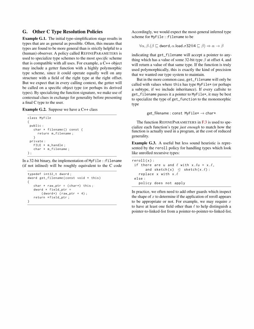
G. Other C Type Resolution PoliciesExample G.1. The initial type-simplification stage results intypes that are as general as possible. Often, this means thattypes are found to be more general than is strictly helpful to a(human) observer. A policy called REFINEPARAMETERS isused to specialize type schemes to the most specific schemethat is compatible with all uses. For example, a C++ objectmay include a getter function with a highly polymorphictype scheme, since it could operate equally well on anystructure with a field of the right type at the right offset.But we expect that in every calling context, the getter willbe called on a specific object type (or perhaps its derivedtypes). By specializing the function signature, we make use ofcontextual clues in exchange for generality before presentinga final C type to the user.

Example G.2. Suppose we have a C++ class

class MyFile{public:

char * filename () const {return m_filename;

}private:

FILE * m_handle;char * m_filename;

};

In a 32-bit binary, the implementation of MyFile::filename(if not inlined) will be roughly equivalent to the C code

typedef int32_t dword;dword get_filename(const void * this){

char * raw_ptr = (char*) this;dword * field_ptr =

(dword*) (raw_ptr + 4);return *field_ptr;

}

Accordingly, we would expect the most-general inferred typescheme for MyFile::filename to be

∀α, β.(β v dword, α.load.σ32@4 v β)⇒ α→ β

indicating that get_filename will accept a pointer to any-thing which has a value of some 32-bit type β at offset 4, andwill return a value of that same type. If the function is trulyused polymorphically, this is exactly the kind of precisionthat we wanted our type system to maintain.

But in the more common case, get_filename will only becalled with values where this has type MyFile* (or perhapsa subtype, if we include inheritance). If every callsite toget_filename passes it a pointer to MyFile*, it may be bestto specialize the type of get_function to the monomorphictype

get_filename : const MyFile*→ char*

The function REFINEPARAMETERS in F.3 is used to spe-cialize each function’s type just enough to match how thefunction is actually used in a program, at the cost of reducedgenerality.

Example G.3. A useful but less sound heuristic is repre-sented by the reroll policy for handling types which looklike unrolled recursive types:

reroll(x):if there are u and ` with x.`u = x.`,

and sketch(x) E sketch(x.`):replace x with x.`

else:policy does not apply

In practice, we often need to add other guards which inspectthe shape of x to determine if the application of reroll appearsto be appropriate or not. For example, we may require xto have at least one field other than ` to help distinguish apointer-to-linked-list from a pointer-to-pointer-to-linked-list.

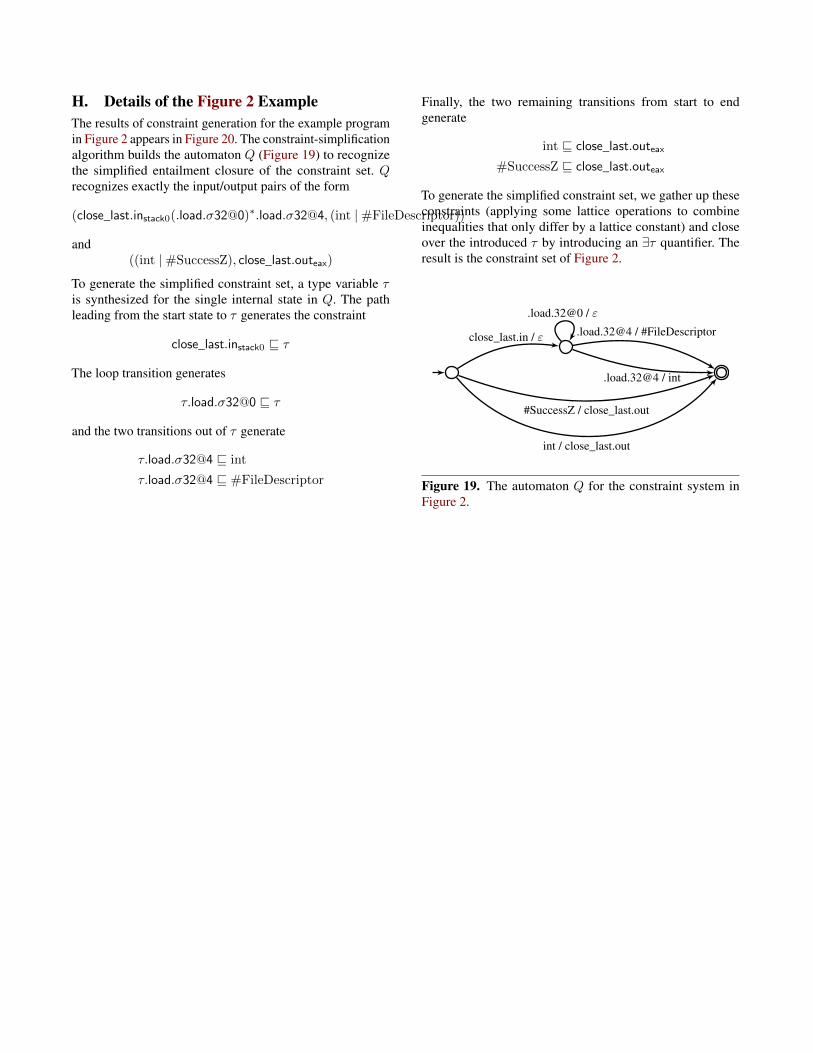
H. Details of the Figure 2 ExampleThe results of constraint generation for the example programin Figure 2 appears in Figure 20. The constraint-simplificationalgorithm builds the automaton Q (Figure 19) to recognizethe simplified entailment closure of the constraint set. Qrecognizes exactly the input/output pairs of the form

(close_last.instack0(.load.σ32@0)∗.load.σ32@4, (int |#FileDescriptor))

and((int |#SuccessZ), close_last.outeax)

To generate the simplified constraint set, a type variable τis synthesized for the single internal state in Q. The pathleading from the start state to τ generates the constraint

close_last.instack0 v τ

The loop transition generates

τ.load.σ32@0 v τ

and the two transitions out of τ generate

τ.load.σ32@4 v int

τ.load.σ32@4 v #FileDescriptor

Finally, the two remaining transitions from start to endgenerate

int v close_last.outeax

#SuccessZ v close_last.outeax

To generate the simplified constraint set, we gather up theseconstraints (applying some lattice operations to combineinequalities that only differ by a lattice constant) and closeover the introduced τ by introducing an ∃τ quantifier. Theresult is the constraint set of Figure 2.

close_last.in / ε .load.32@4 / #FileDescriptor

.load.32@4 / int

#SuccessZ / close_last.out

int / close_last.out

.load.32@0 / ε

Figure 19. The automaton Q for the constraint system inFigure 2.

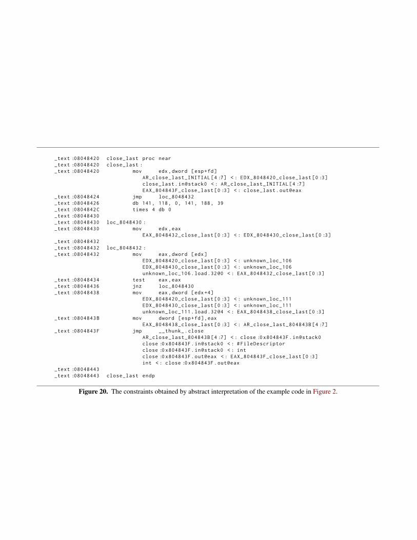
_text :08048420 close_last proc near_text :08048420 close_last:_text :08048420 mov edx ,dword [esp+fd]

AR_close_last_INITIAL [4:7] <: EDX_8048420_close_last [0:3]close_last.in@stack0 <: AR_close_last_INITIAL [4:7]EAX_804843F_close_last [0:3] <: close_last.out@eax

_text :08048424 jmp loc_8048432_text :08048426 db 141, 118, 0, 141, 188, 39_text :0804842C times 4 db 0_text :08048430_text :08048430 loc_8048430:_text :08048430 mov edx ,eax

EAX_8048432_close_last [0:3] <: EDX_8048430_close_last [0:3]_text :08048432_text :08048432 loc_8048432:_text :08048432 mov eax ,dword [edx]

EDX_8048420_close_last [0:3] <: unknown_loc_106EDX_8048430_close_last [0:3] <: unknown_loc_106unknown_loc_106.load .32@0 <: EAX_8048432_close_last [0:3]

_text :08048434 test eax ,eax_text :08048436 jnz loc_8048430_text :08048438 mov eax ,dword [edx+4]

EDX_8048420_close_last [0:3] <: unknown_loc_111EDX_8048430_close_last [0:3] <: unknown_loc_111unknown_loc_111.load .32@4 <: EAX_8048438_close_last [0:3]

_text :0804843B mov dword [esp+fd],eaxEAX_8048438_close_last [0:3] <: AR_close_last_804843B [4:7]

_text :0804843F jmp __thunk_.closeAR_close_last_804843B [4:7] <: close:0 x804843F.in@stack0close:0 x804843F.in@stack0 <: #FileDescriptorclose:0 x804843F.in@stack0 <: intclose:0 x804843F.out@eax <: EAX_804843F_close_last [0:3]int <: close:0 x804843F.out@eax

_text :08048443_text :08048443 close_last endp

Figure 20. The constraints obtained by abstract interpretation of the example code in Figure 2.