115

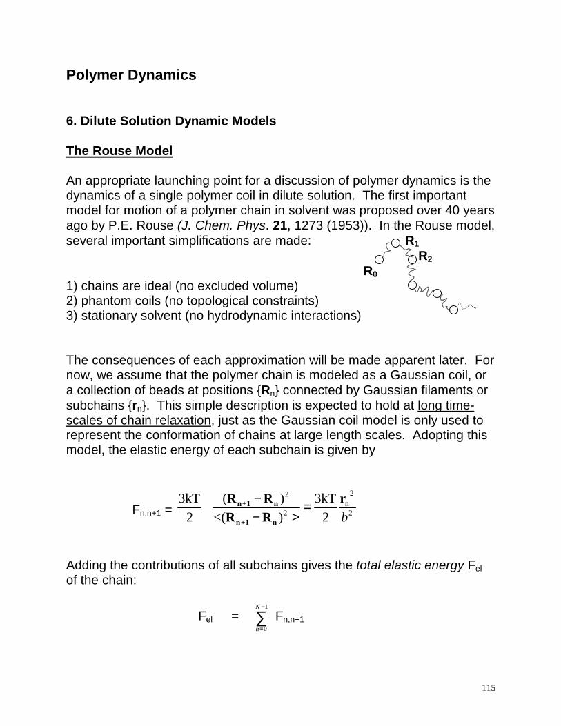
Polymer Dynamics 6. Dilute Solution Dynamic Models The Rouse Model An appropriate launching point for a discussion of polymer dynamics is the dynamics of a single polymer coil in dilute solution. The first important model for motion of a polymer chain in solvent was proposed over 40 years ago by P.E. Rouse (J. Chem. Phys. 21, 1273 (1953)). In the Rouse model, several important simplifications are made: R1

R2 R0 1) chains are ideal (no excluded volume) 2) phantom coils (no topological constraints) 3) stationary solvent (no hydrodynamic interactions) The consequences of each approximation will be made apparent later. For now, we assume that the polymer chain is modeled as a Gaussian coil, or a collection of beads at positions {Rn} connected by Gaussian filaments or subchains {rn}. This simple description is expected to hold at long time-scales of chain relaxation, just as the Gaussian coil model is only used to represent the conformation of chains at large length scales. Adopting this model, the elastic energy of each subchain is given by

Fn,n+1 = 22

n2 2

3kT ( ) 3kT 2 <( ) 2 b

− =− >

n+1 n

n+1 n

R R rR R

Adding the contributions of all subchains gives the total elastic energy Fel of the chain:

Fel = n

N

=

−

∑0

1

Fn,n+1

116

Each bead feels a corresponding elastic force fn,el exerted by its neighbors. For internal beads this force is given by: fn,el = ∂Fel/∂ Rn = 3kT (Rn+1 - 2Rn

+ Rn-1) /b2 n ≠ 0,N while for the end beads:

f0,el = 3kT(R0 - R1) /b2 fN,el = 3kT (RN

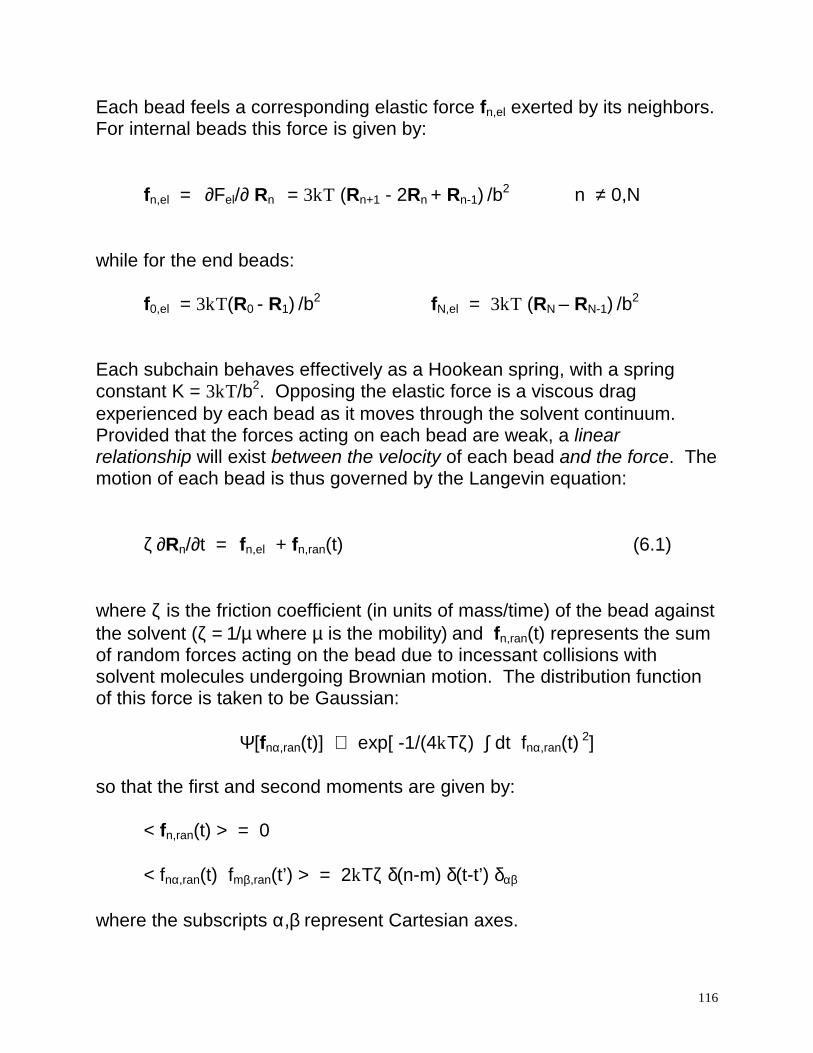
– RN-1) /b2 Each subchain behaves effectively as a Hookean spring, with a spring constant K = 3kT/b2. Opposing the elastic force is a viscous drag experienced by each bead as it moves through the solvent continuum. Provided that the forces acting on each bead are weak, a linear relationship will exist between the velocity of each bead and the force. The motion of each bead is thus governed by the Langevin equation: ζ ∂Rn/∂t = fn,el + fn,ran(t) (6.1) where ζ is the friction coefficient (in units of mass/time) of the bead against the solvent (ζ = 1/µ where µ is the mobility) and fn,ran(t) represents the sum of random forces acting on the bead due to incessant collisions with solvent molecules undergoing Brownian motion. The distribution function of this force is taken to be Gaussian:

Ψ[fnα,ran(t)] ∝ exp[ -1/(4kTζ) ∫ dt fnα,ran(t) 2] so that the first and second moments are given by: < fn,ran(t) > = 0 < fnα,ran(t) fmβ,ran(t’) > = 2kTζ δ(n-m) δ(t-t’) δαβ where the subscripts α,β represent Cartesian axes.

117

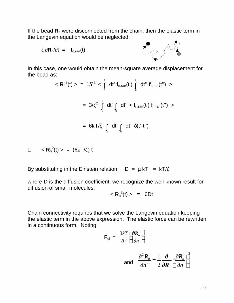
If the bead Rn were disconnected from the chain, then the elastic term in the Langevin equation would be neglected: ζ ∂Rn/∂t = fn,ran(t) In this case, one would obtain the mean-square average displacement for the bead as:

< Rn2(t) > = 1/ζ2 <

0

t

∫ dt’ fn,ran(t’) 0

t

∫ dt’’ fn,ran(t’’) >

= 3/ζ2 0

t

∫ dt’ 0

t

∫ dt’’ < fn,ran(t’) fn,ran(t’’) >

= 6kT/ζ 0

t

∫ dt’ 0

t

∫ dt’’ δ(t’-t’’)

⇒ < Rn

2(t) > = (6kT/ζ) t By substituting in the Einstein relation: D = µ kT = kT/ζ where D is the diffusion coefficient, we recognize the well-known result for diffusion of small molecules:

< Rn2(t) > = 6Dt

Chain connectivity requires that we solve the Langevin equation keeping the elastic term in the above expression. The elastic force can be rewritten in a continuous form. Noting:

Fel = 2

2

32

nkTb n

∂ ∂

R

and 22

2

12

n n

nn n∂ ∂∂ = ∂ ∂ ∂

R RR

118

The elastic force is:

fn,el = ∂Fel/∂Rn = (3kT/b2) ∂2Rn/∂n2

so that the equation of motion becomes: ζ ∂Rn(t)/∂t = K ∂2Rn(t)/∂n2 + fn,ran(t) (6.1a) The equation of motion is solved subject to the boundary conditions: ∂Rn(t)/∂n n=0 = 0 ∂Rn(t)/∂n n=N = 0 (denoting chain ends) One can think of the Langevin equation as describing the Brownian motion of N coupled oscillators. It is useful to recast this equation through a Fourier transformation in n, representing the motion of the chain as a superposition of p independent intra-chain or normal modes. The positional vector is thus represented by a summation of p coordinate vectors Yp(t) (see Appendix 4.II in Doi and Edwards):

Yp(t) = 1/N 0

N

∫ dn cos(πpn/N) Rn(t)

(Note that the F.T. reduces to a cosine transform through the boundary conditions.) The resulting equation of motion is: ζp

∂Yp(t)/∂t = - KpYp(t) + fp,ran(t) (6.2) where ζ0

= Nζ ζp = 2Nζ (p ≠0)

and Kp = 2π2Kp2/N = 6π2 kTp2/Nb2 for p = 0,1,2...

119

and the random force functions

fp,ran(t) = 1/N 0

N

∫ dn cos(πpn/N) fn,ran(t) (6.3)

satisfy:

<fpα,ran(t) > = 0 < fpα,ran(t) fqβ,ran(t’) > = 2 kTζp δpq δ(t-t’) δαβ Since the forces fp,ran(t) are independent of each other, the Langevin equation represents a set of p independent equations, whose solution is given by:

Yp(t) = 1/ζp −∞∫t

dt’ exp[-(t - t’)/ τp)] fp,ran(t’) (6.4)

where τp is the characteristic relaxation time for the pth Rouse mode: τp = ζp /Kp = N2b2ζ/(3π2kTp2) p ≠0 (6.5) Note that for p = 0, the value of the spring constant K0 = 0, so that τ0 = ∞. Physically, p = 0 corresponds to the equation of motion excluding intra-chain relaxation modes: ζ0

∂Y0(t)/∂t = f0,ran(t) (6.6) From the definition of fp,ran(t) given in 6.3, setting p = 0, one can obtain the equality:

ζ0 ∂Y0(t)/∂t = 1/N

0

N

∫ dn fn,ran(t)

= 1/N 0

N

∫ dn ζ ∂Rn/∂t

120

Substituting ζ0 = Nζ and integrating both sides of this equation with respect

to t gives:

Y0(t) = 1/N 0

N

∫ dn Rn(t)

From this result we find that Y0(t) represents the center-of-mass coordinate Rg(t), related to the radius of gyration through:

Rg = < Rg2>1/2

Properties of Rouse Chains Let’s look at the expected properties of the diffusing Rouse chain as a function of time. The mean-square displacement of the coil center of mass is calculated using eq.(6.6) as:

< [Rg(t) - Rg(0)]2 > = 1/ζ02

0

t

∫ dt’ 0

t

∫ dt’’ < f0,ran(t’) f0,ran(t’’) >

= 3/ζ02

0

t

∫ dt’ 0

t

∫ dt’’ < f0,ran(t’) f0,ran(t’’) >

= (6kT/ζN) t (6.7) From this result one can make two primary observations regarding the predictions of the Rouse model: (1) The rms chain displacement scales with time as < ∆Rg

2 >½ ~ t1/2, as with small molecule diffusion.

(2) The mean-square displacement for the polymer coil is reduced by a

factor of 1/N compared with an unconnected bead or small molecule diffusing over the same time frame.

121

The diffusion coefficient for the polymer chain is defined by: Dcoil = lim t→∞ 1/6t < ∆Rg(t)2 > = kT/ζN ~ 1/N From this expression we see that the friction coefficient for the chain is ζeff= ζN, the additive contributions of the N beads. Correspondingly, we can calculate the relaxation of the end-to-end vector R(t) = RN(t) - R0(t). The nth bead position Rn(t) is given by the inverse F.T.: Rn(t) = Y0(t) + 2

p=

∞

∑1

cos(πpn/N) Yp(t) (6.8)

We see that the positional vector for the nth bead is the sum of the center of mass vector plus the superposition of contributions from the p independent intra-chain modes. Hence, we can write R(t) in terms of Yp(t) as: R(t) = -4 ∑ Yp(t) p = 1,3,5... The time correlation for the end-to-end vector is calculated as: < R(t) R(0) > = 16 ∑ < Yp(t) Yp(0) > = 16 ∑ 3kT τp/ζp exp(-t /τp) = 8Nb2/π2 ∑ 1/p2 exp(-t p2/τ1) p = 1,3,5... (6.9) For this expression at t = 0, the summation becomes:

p odd:∑ 1/p2 = π2/8

122

so that we recover for the familiar static value for the mean square end-to-end distance:

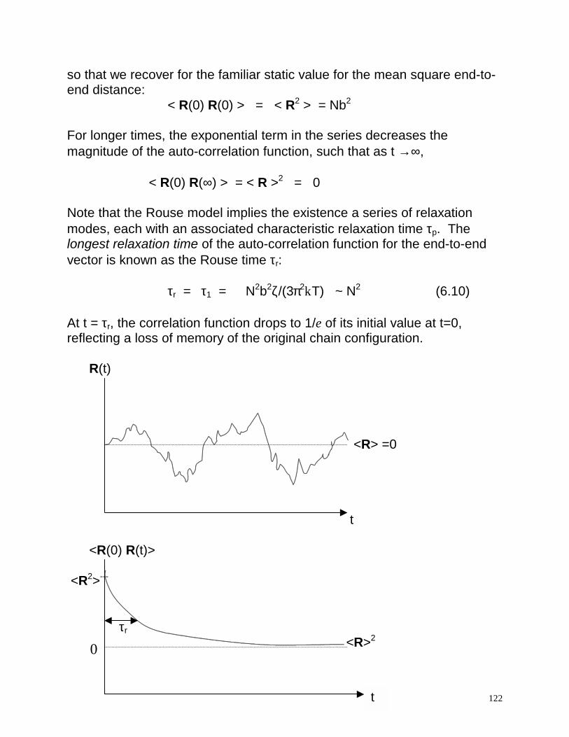
< R(0) R(0) > = < R2 > = Nb2 For longer times, the exponential term in the series decreases the magnitude of the auto-correlation function, such that as t →∞,

< R(0) R(∞) > = < R >2 = 0 Note that the Rouse model implies the existence a series of relaxation modes, each with an associated characteristic relaxation time τp. The longest relaxation time of the auto-correlation function for the end-to-end vector is known as the Rouse time τr:

τr = τ1 = N2b2ζ/(3π2kT) ~ N2 (6.10) At t = τr, the correlation function drops to 1/e of its initial value at t=0, reflecting a loss of memory of the original chain configuration. R(t) <R> =0 t <R(0) R(t)> <R2>---

τr

<R>2

t

0

123

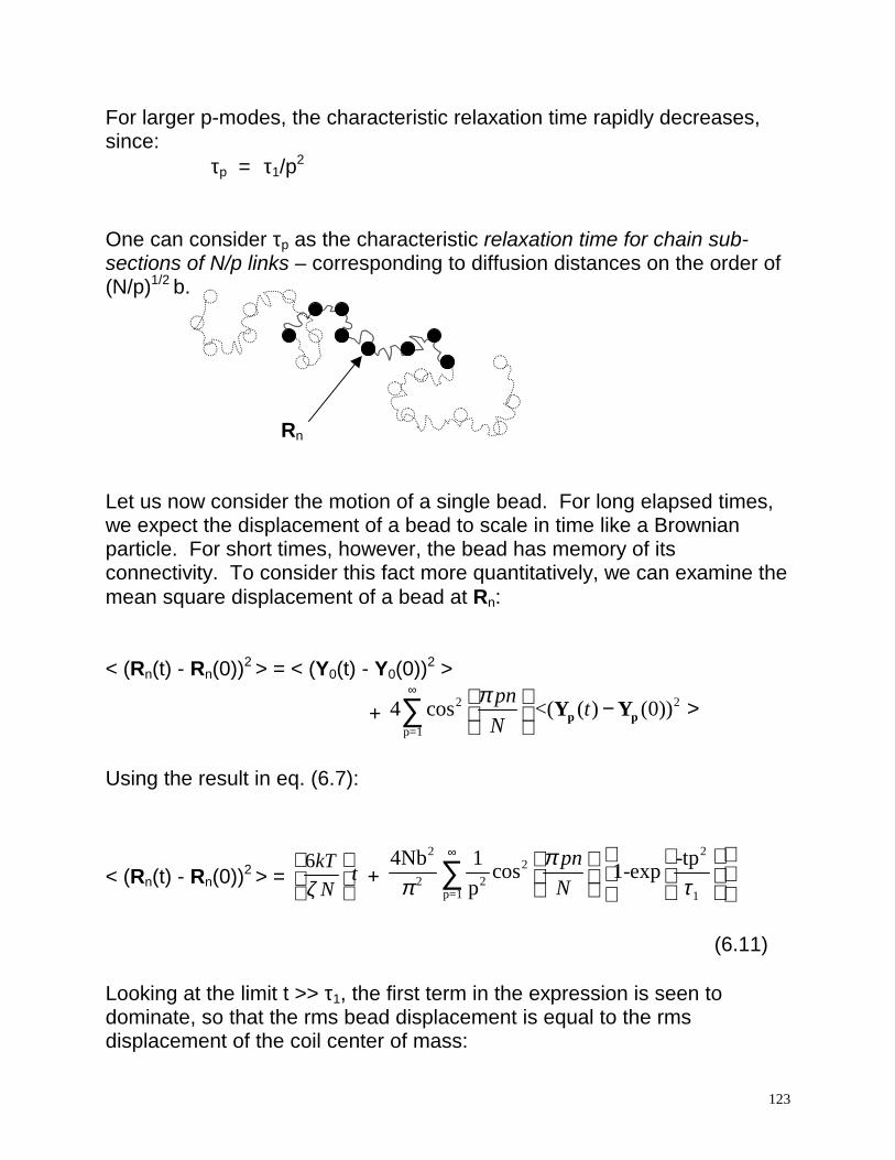
For larger p-modes, the characteristic relaxation time rapidly decreases, since: τp = τ1/p2 One can consider τp as the characteristic relaxation time for chain sub-sections of N/p links – corresponding to diffusion distances on the order of (N/p)1/2 b. Rn Let us now consider the motion of a single bead. For long elapsed times, we expect the displacement of a bead to scale in time like a Brownian particle. For short times, however, the bead has memory of its connectivity. To consider this fact more quantitatively, we can examine the mean square displacement of a bead at Rn: < (Rn(t) - Rn(0))2 > = < (Y0(t) - Y0(0))2 >

+ 2 2

p=14 cos <( ( ) (0)) pn t

Nπ∞ − >

∑ p pY Y

Using the result in eq. (6.7):

< (Rn(t) - Rn(0))2 > = 6kT t

Nζ

+ 2 2

22 2

p=1 1

4Nb 1 -tpcos 1-exp p

pnN

ππ τ

∞

∑

(6.11)

Looking at the limit t >> τ1, the first term in the expression is seen to dominate, so that the rms bead displacement is equal to the rms displacement of the coil center of mass:

124

< (Rn(t) - Rn(0))2 >1/2 ≈ 1/ 2

1/ 26kT tNζ

~ t1/2 (Brownian particle)

For times t << τ1, the expression for the mean square displacement is dominated by large p modes. One can transform the sum to an integral:

< (Rn(t) - Rn(0))2 > 2 2

22 2

10

4Nb 1 -tpdp cos 1-exp p

pnN

ππ τ

∞ ≈ ∫

Replacing the cosine term with its mean value of ½ (justifiable for a rapidly oscillating function), we obtain:

< (Rn(t) - Rn(0))2 > 1/ 22 2 2

1/ 22 2 2

10

2Nb 1 -tp 12kTb1-exp =p

dp tπ τ πζ

∞ ≈

∫

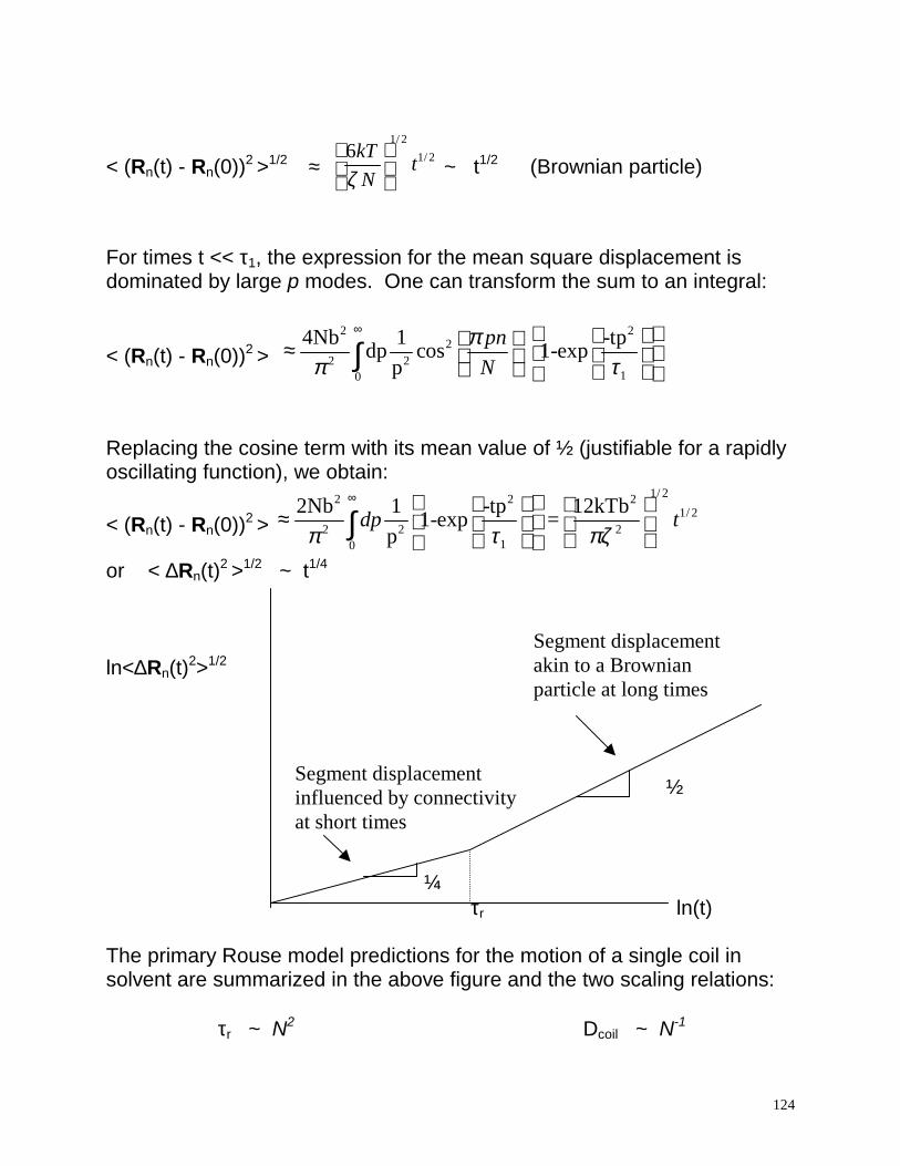
or < ∆Rn(t)2 >1/2 ~ t1/4 ln<∆Rn(t)2>1/2

½ ¼ τr ln(t) The primary Rouse model predictions for the motion of a single coil in solvent are summarized in the above figure and the two scaling relations: τr ~ N2 Dcoil ~ N-1

Segment displacement akin to a Brownian particle at long times

Segment displacement influenced by connectivity at short times

125

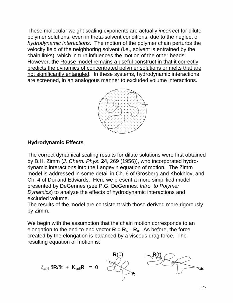
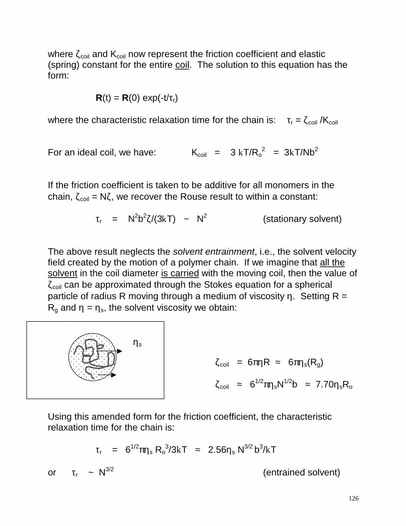
These molecular weight scaling exponents are actually incorrect for dilute polymer solutions, even in theta-solvent conditions, due to the neglect of hydrodynamic interactions. The motion of the polymer chain perturbs the velocity field of the neighboring solvent (i.e., solvent is entrained by the chain links), which in turn influences the motion of the other beads. However, the Rouse model remains a useful construct in that it correctly predicts the dynamics of concentrated polymer solutions or melts that are not significantly entangled. In these systems, hydrodynamic interactions are screened, in an analogous manner to excluded volume interactions. Hydrodynamic Effects The correct dynamical scaling results for dilute solutions were first obtained by B.H. Zimm (J. Chem. Phys. 24, 269 (1956)), who incorporated hydro- dynamic interactions into the Langevin equation of motion. The Zimm model is addressed in some detail in Ch. 6 of Grosberg and Khokhlov, and Ch. 4 of Doi and Edwards. Here we present a more simplified model presented by DeGennes (see P.G. DeGennes, Intro. to Polymer Dynamics) to analyze the effects of hydrodynamic interactions and excluded volume. The results of the model are consistent with those derived more rigorously by Zimm. We begin with the assumption that the chain motion corresponds to an elongation to the end-to-end vector R = RN - R0. As before, the force created by the elongation is balanced by a viscous drag force. The resulting equation of motion is: R(0) R(t) ζcoil ∂R/∂t + KcoilR = 0

126

where ζcoil and Kcoil now represent the friction coefficient and elastic (spring) constant for the entire coil. The solution to this equation has the form:

R(t) = R(0) exp(-t/τr) where the characteristic relaxation time for the chain is: τr = ζcoil /Kcoil For an ideal coil, we have: Kcoil = 3 kT/Ro

2 = 3kT/Nb2

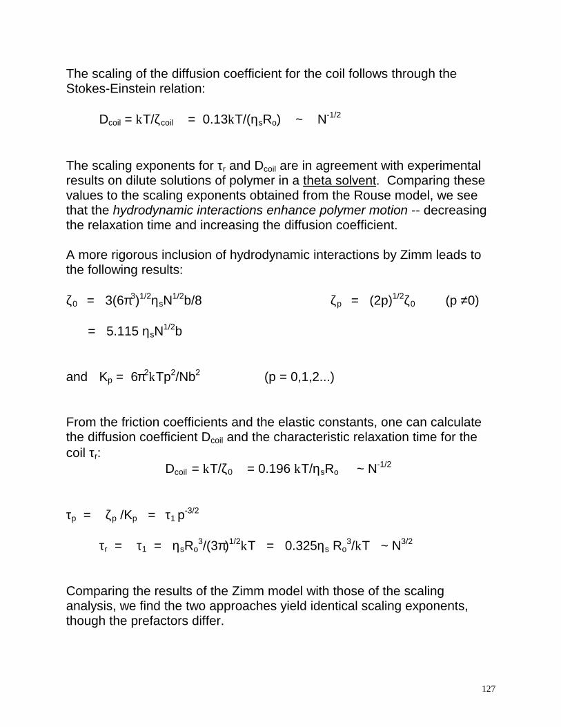
If the friction coefficient is taken to be additive for all monomers in the chain, ζcoil = Nζ, we recover the Rouse result to within a constant: τr = N2b2ζ/(3kT) ~ N2 (stationary solvent) The above result neglects the solvent entrainment, i.e., the solvent velocity field created by the motion of a polymer chain. If we imagine that all the solvent in the coil diameter is carried with the moving coil, then the value of ζcoil can be approximated through the Stokes equation for a spherical particle of radius R moving through a medium of viscosity η. Setting R = Rg and η = ηs, the solvent viscosity we obtain:

ζcoil = 6πηR ≈ 6πηs(Rg) ζcoil ≈ 61/2πηsN1/2b ≈ 7.70ηsRo

Using this amended form for the friction coefficient, the characteristic relaxation time for the chain is: τr = 61/2πηs Ro

3/3kT ≈ 2.56ηs N3/2 b3/kT or τr ~ N3/2 (entrained solvent)

ηs

127

The scaling of the diffusion coefficient for the coil follows through the Stokes-Einstein relation: Dcoil = kT/ζcoil = 0.13kT/(ηsRo) ~ N-1/2 The scaling exponents for τr and Dcoil are in agreement with experimental results on dilute solutions of polymer in a theta solvent. Comparing these values to the scaling exponents obtained from the Rouse model, we see that the hydrodynamic interactions enhance polymer motion -- decreasing the relaxation time and increasing the diffusion coefficient. A more rigorous inclusion of hydrodynamic interactions by Zimm leads to the following results: ζ0

= 3(6π3)1/2ηsN1/2b/8 ζp = (2p)1/2ζ0 (p ≠0)

= 5.115 ηsN1/2b and Kp = 6π2kTp2/Nb2 (p = 0,1,2...) From the friction coefficients and the elastic constants, one can calculate the diffusion coefficient Dcoil and the characteristic relaxation time for the coil τr:

Dcoil = kT/ζ0 = 0.196 kT/ηsRo ~ N-1/2 τp = ζp /Kp = τ1 p-3/2

τr = τ1 = ηsRo

3/(3π)1/2kT = 0.325ηs Ro3/kT ~ N3/2

Comparing the results of the Zimm model with those of the scaling analysis, we find the two approaches yield identical scaling exponents, though the prefactors differ.

128

Excluded Volume Effects The scaling analysis can be easily modified to incorporate the effects of excluded volume for chains in good solvents. Exchanging Ro for the characteristic swollen coil dimension, RF = N3/5b, we obtain the scaling results:

Dcoil ~ kT/(ηsRF) ~ N-3/5 (swollen coil, entrained solvent)

τr ~ ηs RF3/kT ~ N9/5

Accounting for prefactors, the results for Dcoil are: Dcoil = kT/ζcoil ≈ kT/(6πηs(RF/√7))

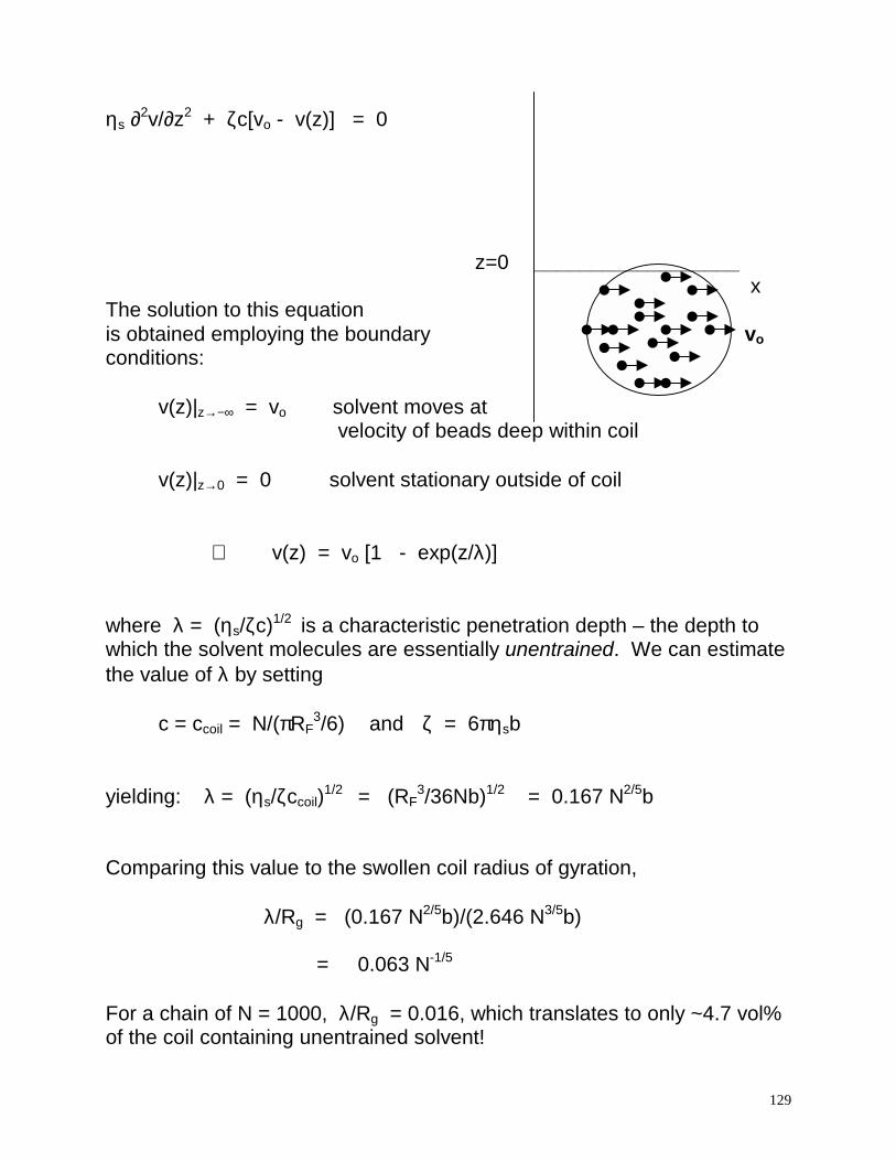
= 0.140 kT/ηsRF (DeGennes scaling) More rigorously: Dcoil = kT/ζ0 ≈ 0.083 kT/ηsRF (RG result of Oono) It may seem somewhat unintuitive that the volume of solvent within the coil should move along with the coil as it diffuses, particularly for large swollen coils where the coil density is sparse. To see why this is nevertheless the case, we can make a simple estimation of the velocity distribution of the solvent within the moving coil (see Grosberg and Khokhlov, pg. 238). We imagine that we have a half-space z<0 which contains a concentration c of beads, each moving with a velocity vo in the x direction, and having a frictional coefficient with the solvent ζ. The frictional force exerted on the neighboring solvent molecules is consequently given by ζ(vo - v). The corresponding Navier-Stokes equation, neglecting inertial effects and assuming a weak perturbation on the velocity, becomes:

129

ηs ∂2v/∂z2 + ζc[vo - v(z)] = 0 z=0 __________________ x The solution to this equation is obtained employing the boundary vo conditions:

v(z)|z→−∞ = vo solvent moves at velocity of beads deep within coil

v(z)|z→0 = 0 solvent stationary outside of coil ⇒ v(z) = vo [1 - exp(z/λ)] where λ = (ηs/ζc)1/2 is a characteristic penetration depth – the depth to which the solvent molecules are essentially unentrained. We can estimate the value of λ by setting

c = ccoil = N/(πRF3/6) and ζ = 6πηsb

yielding: λ = (ηs/ζccoil)1/2 = (RF

3/36Nb)1/2 = 0.167 N2/5b Comparing this value to the swollen coil radius of gyration, λ/Rg = (0.167 N2/5b)/(2.646 N3/5b) = 0.063 N-1/5 For a chain of N = 1000, λ/Rg = 0.016, which translates to only ~4.7 vol% of the coil containing unentrained solvent!

130

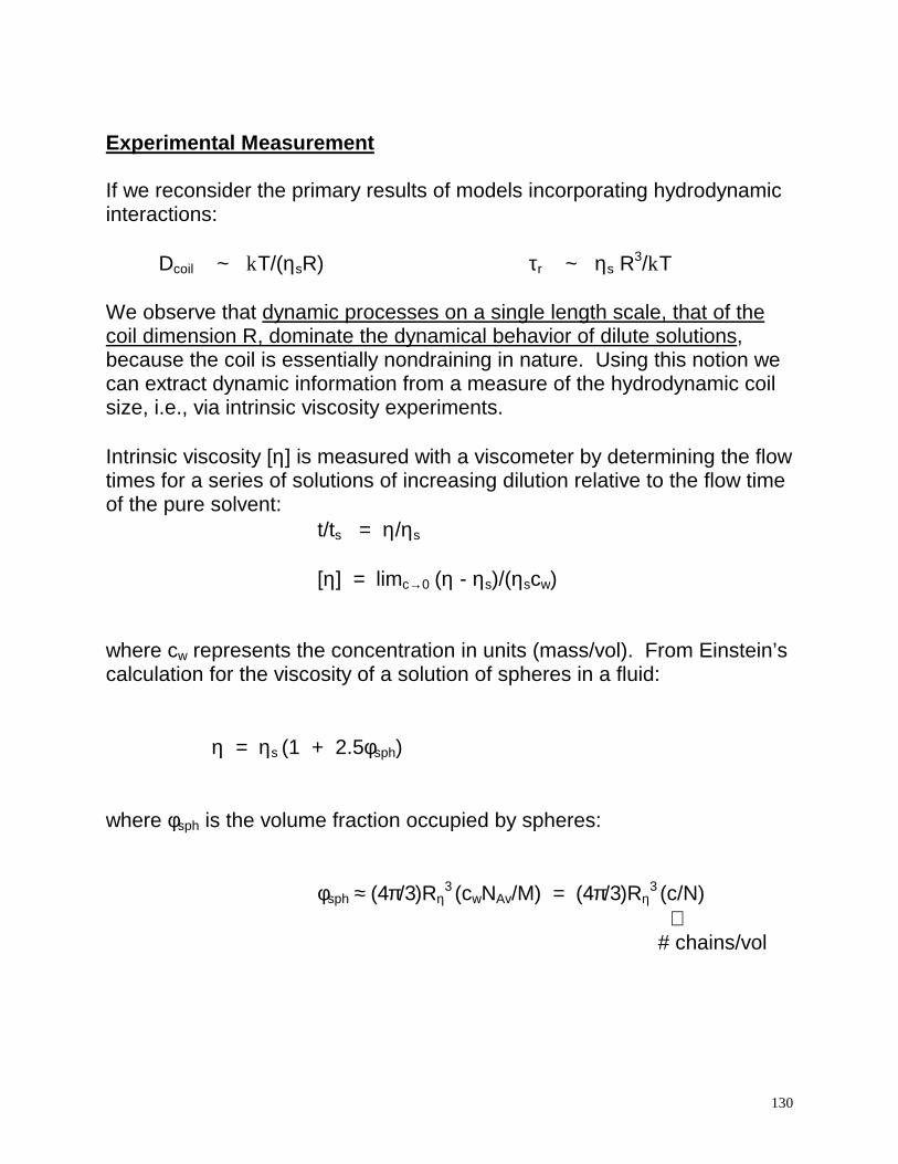
Experimental Measurement If we reconsider the primary results of models incorporating hydrodynamic interactions:

Dcoil ~ kT/(ηsR) τr ~ ηs R3/kT We observe that dynamic processes on a single length scale, that of the coil dimension R, dominate the dynamical behavior of dilute solutions, because the coil is essentially nondraining in nature. Using this notion we can extract dynamic information from a measure of the hydrodynamic coil size, i.e., via intrinsic viscosity experiments. Intrinsic viscosity [η] is measured with a viscometer by determining the flow times for a series of solutions of increasing dilution relative to the flow time of the pure solvent: t/ts = η/ηs

[η] = limc→0 (η - ηs)/(ηscw) where cw represents the concentration in units (mass/vol). From Einstein’s calculation for the viscosity of a solution of spheres in a fluid: η = ηs (1 + 2.5φsph) where φsph is the volume fraction occupied by spheres:

φsph ≈ (4π/3)Rη3 (cwNAv/M) = (4π/3)Rη

3 (c/N)

⇑ # chains/vol

131

where Rη is the hydrodynamic radius, M is molecular weight and NAv is Avogadro’s number. From this we obtain the relation between intrinsic viscosity and Rη : [η] = (10π/3)Rη

3 (NAv/M)

A priori knowledge of molecular weight allows one to calculate the value of Rη. The intrinsic viscosity is also expected to scale with N (or M) as: [η] = const Rη

3/N [η] ~ N1/2 (Θ-solvent) [η] ~ N4/5 (good solvent) We can also relate τr to experimental measurements of the intrinsic viscosity: τr = const [η] ηsM/(NAvkT) while the relaxation time and the chain diffusion coefficient are related through:

Dcoil ~ R2/τr A more rigorous statistical mechanical calculation of [η] is described in Ch. 6 of Grosberg and Khokhlov and Doi and Edwards pp. 112-116. In that analysis, the Langevin equation is amended to take into account the additional velocity of a segment Rn due to the velocity field created by shear. For polymer solutions, the intrinsic viscosity is obtained as: [η] = NAvkT/(M ηs)

p=

∞

∑1

τp/2

where the τp are the (model dependent) characteristic relaxation times.

132

For the Rouse model, recall that τp = τ1/p2, giving [η] = (NAv/Mηs) (N2b2ζ/6π2)

p=

∞

∑1

1/p2

Since

p=

∞

∑1

1/p2 = π2/6 , [η] = (NAv/Mηs) (N2b2ζ/36) ~ N

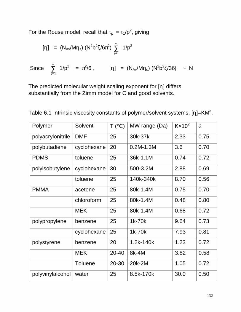
The predicted molecular weight scaling exponent for [η] differs substantially from the Zimm model for Θ and good solvents. Table 6.1 Intrinsic viscosity constants of polymer/solvent systems, [η]=KMa.

Polymer Solvent T (°C) MW range (Da) K×102 a

polyacrylonitrile DMF 25 30k-37k 2.33 0.75

polybutadiene cyclohexane 20 0.2M-1.3M 3.6 0.70

PDMS toluene 25 36k-1.1M 0.74 0.72

polyisobutylene cyclohexane 30 500-3.2M 2.88 0.69

toluene 25 140k-340k 8.70 0.56

PMMA acetone 25 80k-1.4M 0.75 0.70

chloroform 25 80k-1.4M 0.48 0.80

MEK 25 80k-1.4M 0.68 0.72

polypropylene benzene 25 1k-70k 9.64 0.73

cyclohexane 25 1k-70k 7.93 0.81

polystyrene benzene 20 1.2k-140k 1.23 0.72

MEK 20-40 8k-4M 3.82 0.58

Toluene 20-30 20k-2M 1.05 0.72

polyvinylalcohol water 25 8.5k-170k 30.0 0.50

133

7. Concentrated Solutions and Melts As chains are added to the solvent beyond the overlap concentration c*, a rapid increase in the solution viscosity is observed (with a subsequent drop in the magnitude of the diffusion coefficient). Other chains penetrate the coil volume of a given chain, placing topological constraints on its motion. In a polymer melt, the viscosity is experimentally seen to have two scaling regimes in molecular weight:

η ~ M M < Mc

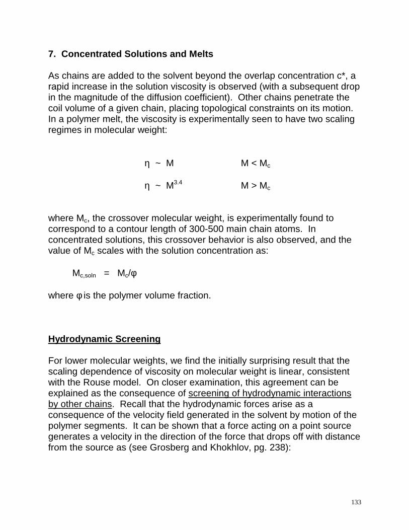
η ~ M3.4 M > Mc where Mc, the crossover molecular weight, is experimentally found to correspond to a contour length of 300-500 main chain atoms. In concentrated solutions, this crossover behavior is also observed, and the value of Mc scales with the solution concentration as: Mc,soln = Mc/φ where φ is the polymer volume fraction. Hydrodynamic Screening For lower molecular weights, we find the initially surprising result that the scaling dependence of viscosity on molecular weight is linear, consistent with the Rouse model. On closer examination, this agreement can be explained as the consequence of screening of hydrodynamic interactions by other chains. Recall that the hydrodynamic forces arise as a consequence of the velocity field generated in the solvent by motion of the polymer segments. It can be shown that a force acting on a point source generates a velocity in the direction of the force that drops off with distance from the source as (see Grosberg and Khokhlov, pg. 238):

134

v(r) ~ 1/ηs r f r As the viscosity of the solution increases with the addition of polymer chains melt, this velocity becomes:

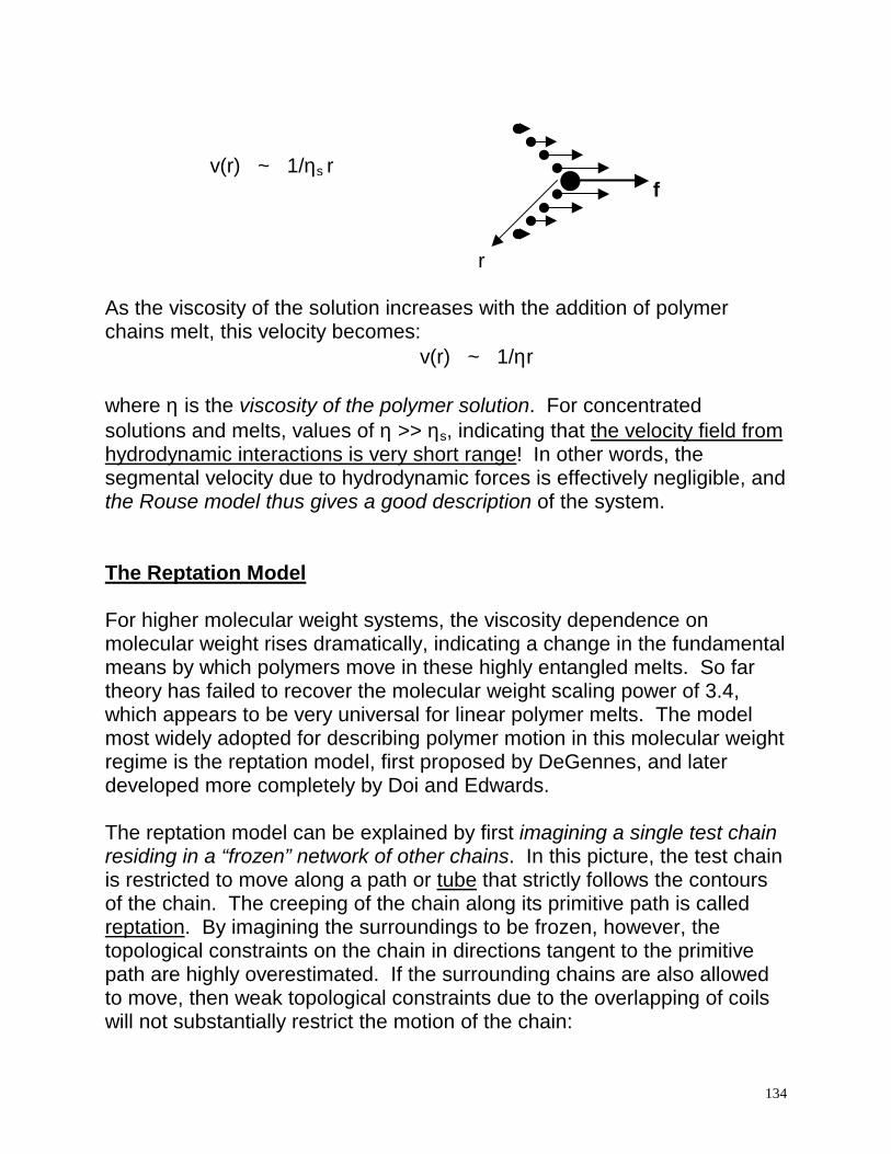
v(r) ~ 1/ηr where η is the viscosity of the polymer solution. For concentrated solutions and melts, values of η >> ηs, indicating that the velocity field from hydrodynamic interactions is very short range! In other words, the segmental velocity due to hydrodynamic forces is effectively negligible, and the Rouse model thus gives a good description of the system. The Reptation Model For higher molecular weight systems, the viscosity dependence on molecular weight rises dramatically, indicating a change in the fundamental means by which polymers move in these highly entangled melts. So far theory has failed to recover the molecular weight scaling power of 3.4, which appears to be very universal for linear polymer melts. The model most widely adopted for describing polymer motion in this molecular weight regime is the reptation model, first proposed by DeGennes, and later developed more completely by Doi and Edwards. The reptation model can be explained by first imagining a single test chain residing in a “frozen” network of other chains. In this picture, the test chain is restricted to move along a path or tube that strictly follows the contours of the chain. The creeping of the chain along its primitive path is called reptation. By imagining the surroundings to be frozen, however, the topological constraints on the chain in directions tangent to the primitive path are highly overestimated. If the surrounding chains are also allowed to move, then weak topological constraints due to the overlapping of coils will not substantially restrict the motion of the chain:

135

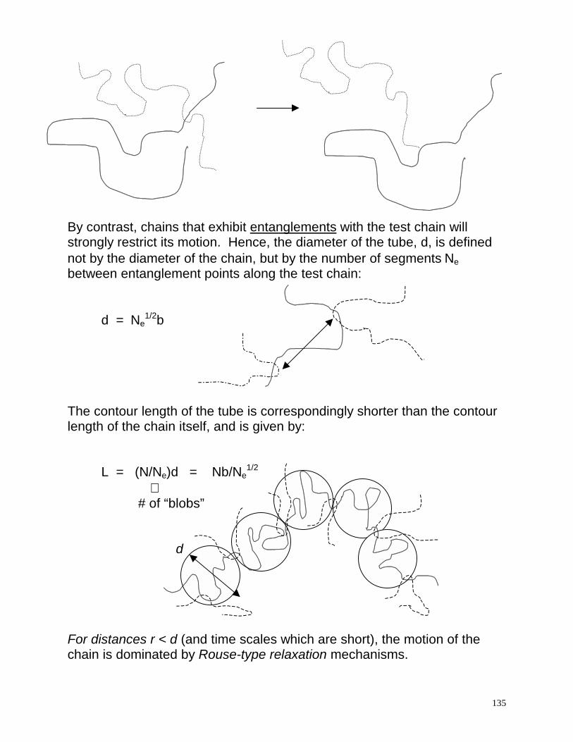
By contrast, chains that exhibit entanglements with the test chain will strongly restrict its motion. Hence, the diameter of the tube, d, is defined not by the diameter of the chain, but by the number of segments Ne between entanglement points along the test chain: d = Ne

1/2b The contour length of the tube is correspondingly shorter than the contour length of the chain itself, and is given by: L = (N/Ne)d = Nb/Ne

1/2 ⇑ # of “blobs” d For distances r < d (and time scales which are short), the motion of the chain is dominated by Rouse-type relaxation mechanisms.

136

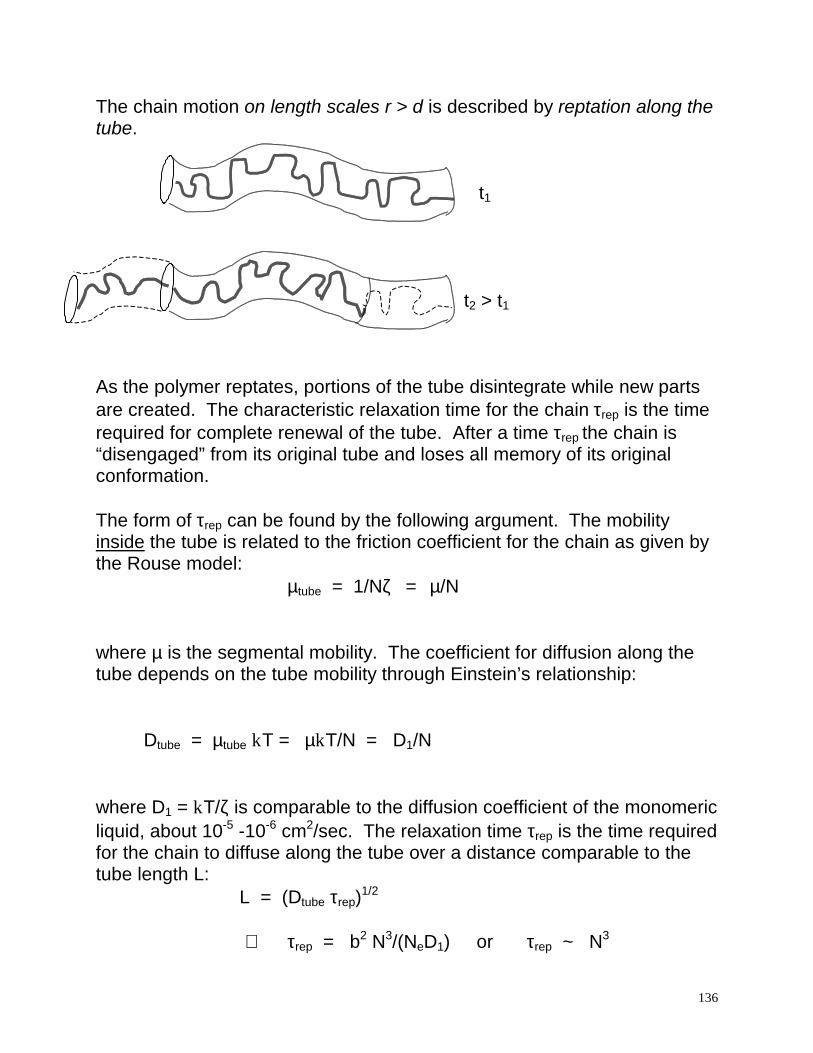
The chain motion on length scales r > d is described by reptation along the tube.

t1 t2 > t1 As the polymer reptates, portions of the tube disintegrate while new parts are created. The characteristic relaxation time for the chain τrep is the time required for complete renewal of the tube. After a time τrep the chain is “disengaged” from its original tube and loses all memory of its original conformation. The form of τrep can be found by the following argument. The mobility inside the tube is related to the friction coefficient for the chain as given by the Rouse model:

µtube = 1/Nζ = µ/N where µ is the segmental mobility. The coefficient for diffusion along the tube depends on the tube mobility through Einstein’s relationship: Dtube = µtube kT = µkT/N = D1/N where D1 = kT/ζ is comparable to the diffusion coefficient of the monomeric liquid, about 10-5 -10-6 cm2/sec. The relaxation time τrep is the time required for the chain to diffuse along the tube over a distance comparable to the tube length L:

L = (Dtube τrep)1/2 ⇒ τrep = b2 N3/(NeD1) or τrep ~ N3

137

This result compares well to the experimentally observed scaling result of 3.4 obtained through dynamic mechanical measurements, discussed more below. In the time τrep the reptating chain moves along the tube by a length L, but in space its displacement is much shorter, on the order of Ro = N1/2b. Hence the diffusion coefficient for the coil is much smaller, and is given by the relation:

Ro = (Dcoil τrep)1/2 ⇒ Dcoil = D1Ne/N2 or Dcoil ~ N-2 This scaling has been experimentally observed for linear chains, and in computer simulations. A more rigorous calculation for the coil diffusion coefficient leads to: Dcoil = D1Ne/3N2 and τrep = b4N3ζ/π2kTd2 Properties of Reptating Chains Time correlation functions can be obtained for the reptation model by solving the equation of motion for the curvilinear coordinates sn(t) of the nth bead along the primitive path of the tube (referenced from an origin point). O sn

The mathematics is analogous to that used to characterize the motion of the segmental coordinate Rn in the Rouse model described earlier.

138

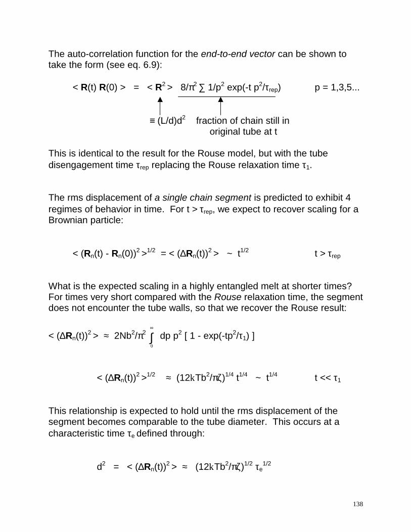
The auto-correlation function for the end-to-end vector can be shown to take the form (see eq. 6.9): < R(t) R(0) > = < R2 > 8/π2 ∑ 1/p2 exp(-t p2/τrep) p = 1,3,5... ≡ (L/d)d2 fraction of chain still in

original tube at t This is identical to the result for the Rouse model, but with the tube disengagement time τrep replacing the Rouse relaxation time τ1. The rms displacement of a single chain segment is predicted to exhibit 4 regimes of behavior in time. For t > τrep, we expect to recover scaling for a Brownian particle: < (Rn(t) - Rn(0))2 >1/2 = < (∆Rn(t))2 > ~ t1/2 t > τrep What is the expected scaling in a highly entangled melt at shorter times? For times very short compared with the Rouse relaxation time, the segment does not encounter the tube walls, so that we recover the Rouse result:

< (∆Rn(t))2 > ≈ 2Nb2/π2 0

∞

∫ dp p2 [ 1 - exp(-tp2/τ1) ]

< (∆Rn(t))2 >1/2 ≈ (12kTb2/πζ)1/4 t1/4 ~ t1/4 t << τ1 This relationship is expected to hold until the rms displacement of the segment becomes comparable to the tube diameter. This occurs at a characteristic time τe

defined through:

d2 = < (∆Rn(t))2 > ≈ (12kTb2/πζ)1/2 τe1/2

139

or τe ≈ πd4ζ/(12kTb2) ~ N0

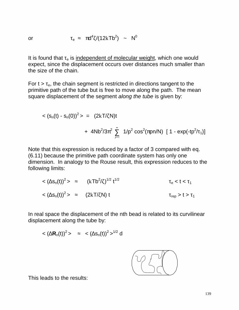
It is found that τe is independent of molecular weight, which one would expect, since the displacement occurs over distances much smaller than the size of the chain. For t > τe, the chain segment is restricted in directions tangent to the primitive path of the tube but is free to move along the path. The mean square displacement of the segment along the tube is given by:

< (sn(t) - sn(0))2 > = (2kT/ζN)t

+ 4Nb2/3π2

p=

∞

∑1

1/p2 cos2(πpn/N) [ 1 - exp(-tp2/τ1)]

Note that this expression is reduced by a factor of 3 compared with eq. (6.11) because the primitive path coordinate system has only one dimension. In analogy to the Rouse result, this expression reduces to the following limits: < (∆sn(t))2 > ≈ (kTb2/ζ)1/2 t1/2 τe < t < τ1 < (∆sn(t))2 > ≈ (2kT/ζN) t τrep > t > τ1 In real space the displacement of the nth bead is related to its curvilinear displacement along the tube by: < (∆Rn(t))2 > ≈ < (∆sn(t))2 >1/2 d This leads to the results:

140

d2

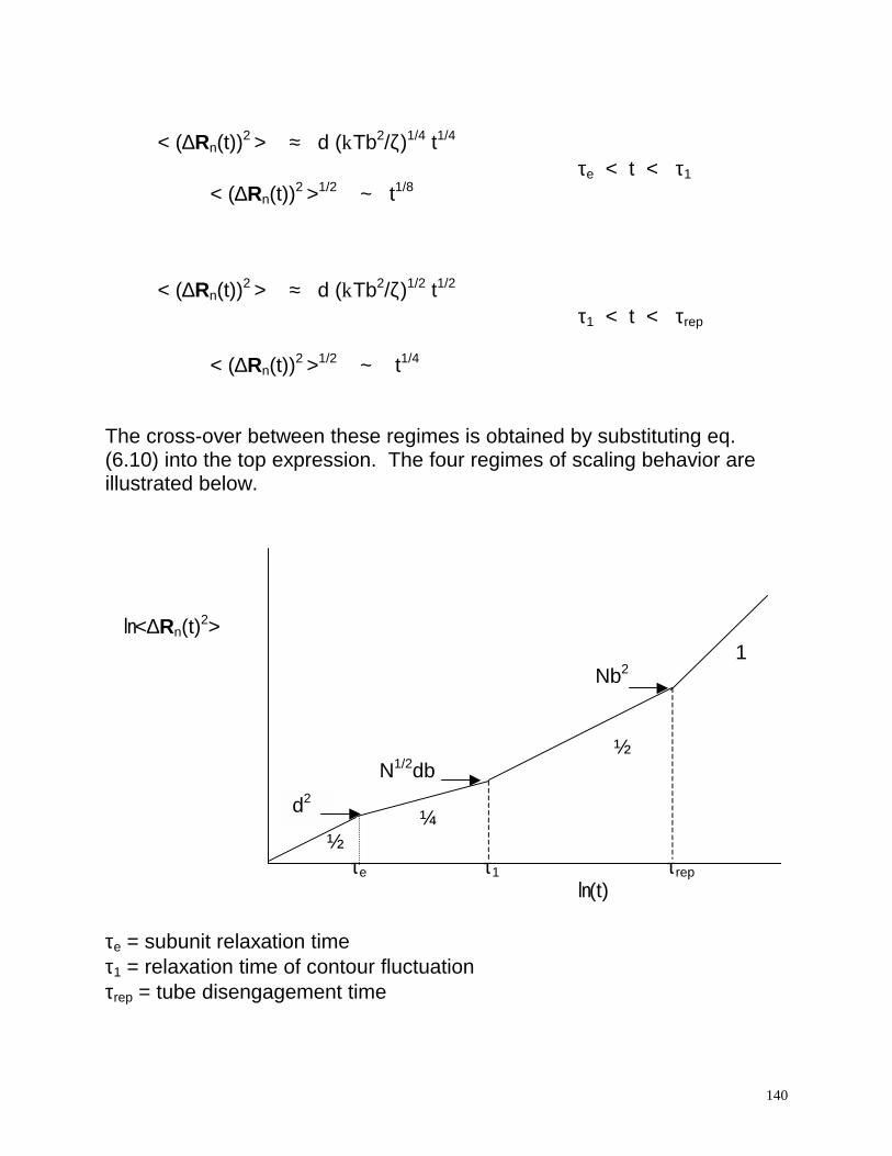
< (∆Rn(t))2 > ≈ d (kTb2/ζ)1/4 t1/4

τe < t < τ1 < (∆Rn(t))2 >1/2 ~ t1/8 < (∆Rn(t))2 > ≈ d (kTb2/ζ)1/2 t1/2

τ1 < t < τrep

< (∆Rn(t))2 >1/2 ~ t1/4 The cross-over between these regimes is obtained by substituting eq. (6.10) into the top expression. The four regimes of scaling behavior are illustrated below. ln<∆Rn(t)2>

1 Nb2

½ N1/2db

¼

½ τe τ1 τrep

ln(t) τe = subunit relaxation time τ1 = relaxation time of contour fluctuation τrep = tube disengagement time

141

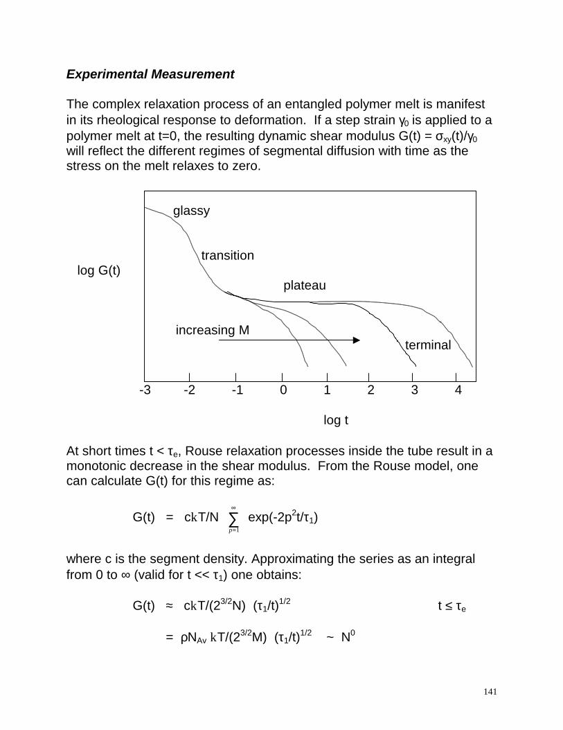
Experimental Measurement The complex relaxation process of an entangled polymer melt is manifest in its rheological response to deformation. If a step strain γ0 is applied to a polymer melt at t=0, the resulting dynamic shear modulus G(t) = σxy(t)/γ0 will reflect the different regimes of segmental diffusion with time as the stress on the melt relaxes to zero.

glassy transition log G(t)

plateau

increasing M

terminal -3 -2 -1 0 1 2 3 4

log t At short times t < τe, Rouse relaxation processes inside the tube result in a monotonic decrease in the shear modulus. From the Rouse model, one can calculate G(t) for this regime as: G(t) = ckT/N

p=

∞

∑1

exp(-2p2t/τ1)

where c is the segment density. Approximating the series as an integral from 0 to ∞ (valid for t << τ1) one obtains: G(t) ≈ ckT/(23/2N) (τ1/t)1/2 t ≤ τe = ρNAv kT/(23/2M) (τ1/t)1/2 ~ N0

142

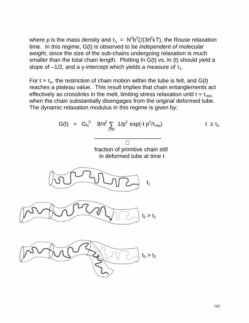
where ρ is the mass density and τ1 = N2b2ζ/(3π2kT), the Rouse relaxation time. In this regime, G(t) is observed to be independent of molecular weight, since the size of the sub-chains undergoing relaxation is much smaller than the total chain length. Plotting ln G(t) vs. ln (t) should yield a slope of –1/2, and a y-intercept which yields a measure of τ1. For t > τe, the restriction of chain motion within the tube is felt, and G(t) reaches a plateau value. This result implies that chain entanglements act effectively as crosslinks in the melt, limiting stress relaxation until t ≈ τrep, when the chain substantially disengages from the original deformed tube. The dynamic relaxation modulus in this regime is given by:

G(t) = GN0 8/π2

p odd:∑ 1/p2 exp(-t p2/τrep) t ≥ τe

_____________________ ⇑ fraction of primitive chain still

in deformed tube at time t

t1 t2 > t1 t3 > t2

143

The factor GN0 is the plateau modulus. It can be calculated by setting t = τe

in the Rouse expression for G(t), denoting the crossover between the two regimes:

GN0 = G(τe) = ckT/(23/2N) (τ1/τe)1/2

Substituting the expressions for τ1 and τe gives (neglecting prefactors):

GN

0 ~ ckT (b/d)2 = ckT/Ne

= NAvρkT/Me The magnitude of GN

0 is again seen to be independent of chain molecular weight, but gives a measure of the entanglement molecular weight Me, or the tube diameter, d = Ne

1/2b = (MeN/M)1/2b = < RMe 2>1/2

If N is large, the value of G(t) for t > τe remains roughly equal to GN

0 over many time decades. The slowest relaxation time dominates the stress relaxation behavior. The leading contribution to G(t) is for p=1, with a characteristic relaxation time equal to the reptation time: τrep = N2b4ζ/(π2d2kT) = τ1 3Nb2/d2 = τ1 3N/Ne G(τrep) ≈ GN

0/e = 0.368 GN0

or on a log-log plot:

ln G(τrep) ≈ ln GN0 - 1

144

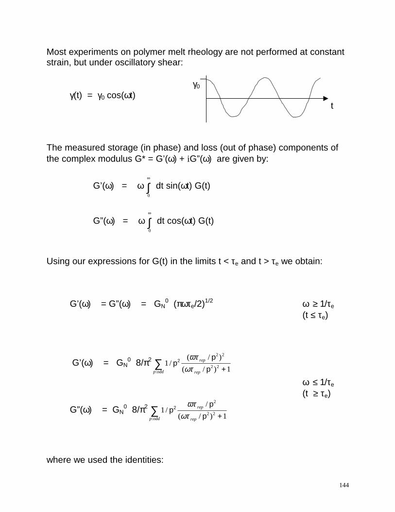
Most experiments on polymer melt rheology are not performed at constant strain, but under oscillatory shear:

γ0 γ(t) = γ0 cos(ωt)

t The measured storage (in phase) and loss (out of phase) components of the complex modulus G* = G’(ω) + iG”(ω) are given by:

G’(ω) = ω 0

∞

∫ dt sin(ωt) G(t)

G”(ω) = ω 0

∞

∫ dt cos(ωt) G(t)

Using our expressions for G(t) in the limits t < τe and t > τe we obtain:

G’(ω) = G”(ω) = GN0 (πωτe/2)1/2 ω ≥ 1/τe

(t ≤ τe)

G’(ω) = GN0 8/π2 1

1

2

2 2/( / )

( / ):

pp

p2 ϖτ

ωτrep

repp odd

2

+∑

ω ≤ 1/τe (t ≥ τe)

G”(ω) = GN0 8/π2 1

12 2//

( / ):

pp

p2 ϖτ

ωτrep

repp odd

2

+∑

where we used the identities:

145

0

∞

∫ dx sin(x)/x1/2 = 0

∞

∫ dx cos(x)/xn = (π/2)1/2

0

∞

∫ dx exp(-ax) sin(bx) = ba b2 2+

0

∞

∫ dx exp(-ax) cos(bx) = aa b2 2+

and substituted: GN

0τe1/2 = ckT/(23/2N) τ1

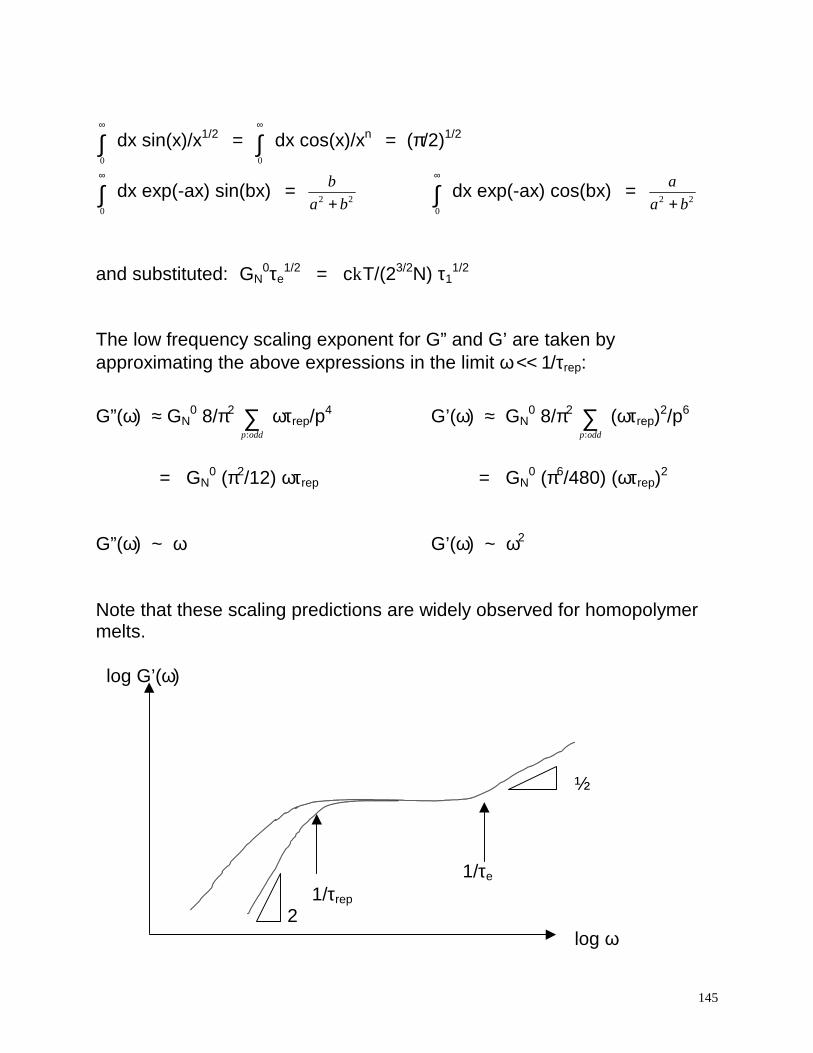
1/2 The low frequency scaling exponent for G” and G’ are taken by approximating the above expressions in the limit ω << 1/τrep:

G”(ω) ≈ GN0 8/π2

p odd:∑ ωτrep/p4 G’(ω) ≈ GN

0 8/π2

p odd:∑ (ωτrep)2/p6

= GN

0 (π2/12) ωτrep = GN0 (π6/480) (ωτrep)2

G”(ω) ~ ω G’(ω) ~ ω2

Note that these scaling predictions are widely observed for homopolymer melts. log G’(ω)

½

1/τe 1/τrep

2 log ω

146

The zero shear viscosity is related to the shear modulus through:

η = 0

∞

∫ dt G(t) = limω→0 G”(ω)

η = GN0 8/π2

0

∞

∫ dt p odd:∑ 1/p2 exp(-t p2/τrep)

= GN0 8/π2

p odd:∑ τrep/p4

⇒ η = GN0 (π2/12) τrep ~ N3

Other Relaxation Modes While the reptation model captures the essence of the behavior for entangled polymer melts, there are several important discrepencies between the theoretical predictions and experimental observations. One significant discrepency is that the scaling exponent for the viscosity with molecular weight is underestimated. In addition, the calculated viscosity and relaxation time are significantly larger than observed values, while Mc is two to three times larger than Me. The empirically observed behavior for viscosity is:

η(exp)(M) = η(Mc) (M/Mc)3.4 M > Mc By comparison, the theoretical viscosity can be written as:

η(theo)(M) = 15/4 η(Me) (M/Me)3 M > Me

The predicted viscosity is ~ 15 times larger than the observed viscosity at Mc.

147

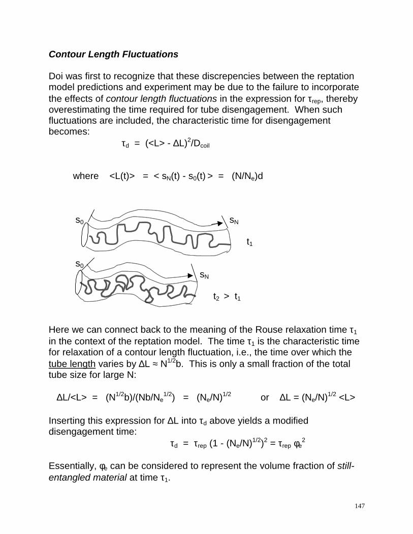
Contour Length Fluctuations Doi was first to recognize that these discrepencies between the reptation model predictions and experiment may be due to the failure to incorporate the effects of contour length fluctuations in the expression for τrep, thereby overestimating the time required for tube disengagement. When such fluctuations are included, the characteristic time for disengagement becomes: τd = (<L> - ∆L)2/Dcoil

where <L(t)> = < sN(t) - s0(t) > = (N/Ne)d s0 sN

t1 s0 sN t2 > t1 Here we can connect back to the meaning of the Rouse relaxation time τ1 in the context of the reptation model. The time τ1 is the characteristic time for relaxation of a contour length fluctuation, i.e., the time over which the tube length varies by ∆L ≈ N1/2b. This is only a small fraction of the total tube size for large N: ∆L/<L> = (N1/2b)/(Nb/Ne

1/2) = (Ne/N)1/2 or ∆L = (Ne/N)1/2 <L> Inserting this expression for ∆L into τd above yields a modified disengagement time:

τd = τrep (1 - (Ne/N)1/2)2 = τrep φe2

Essentially, φe can be considered to represent the volume fraction of still-entangled material at time τ1.

148

The contour length fluctuations decrease the disengagement time significantly, similarly decreasing the predicted viscosity, and modifying its molecular weight dependence. A modified expression for the late-time shear modulus can thus be written taking into account this revised disengagement time:

G(t) = GN0 8/π2

p odd:∑ 1/p2 exp(-t p2/τd)

It has most recently been recognized that the prefactor GN

0 must also be revised to account for the “dynamic dilution” of entanglements in the expression for the plateau modulus. This modification (see Milner and McLeish, Phys Rev Lett. 81, 725 (1998)) arises from the dependence of GN

0 on the molecular weight between entanglements Ne and segment density c:

GN

0 = ckT/Ne Assuming a dilution of melt segment density and an increase in the molecular weight between entanglements due to early stage relaxation processes: c(τ1) = c φe and Ne(τ1) = Ne/φe leads to an effective plateau modulus:

GN0(τ1) = GN

0 φe2

Which should be substituted into the above expression for G(t).

149

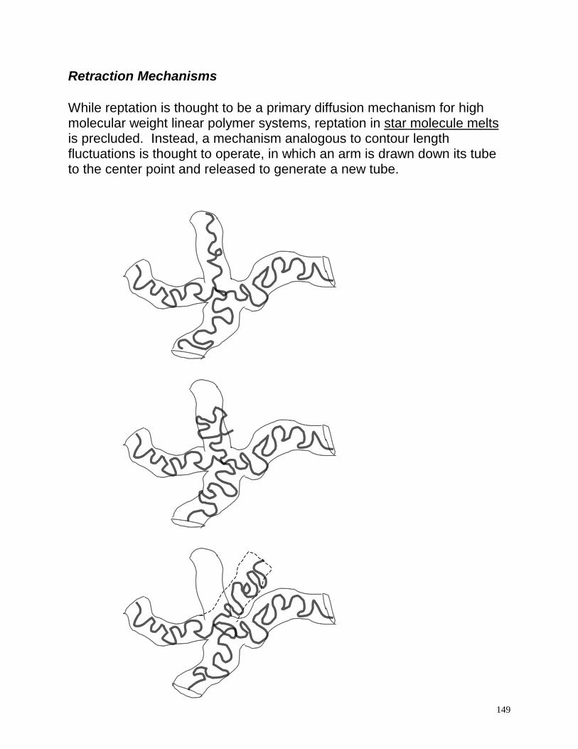
Retraction Mechanisms While reptation is thought to be a primary diffusion mechanism for high molecular weight linear polymer systems, reptation in star molecule melts is precluded. Instead, a mechanism analogous to contour length fluctuations is thought to operate, in which an arm is drawn down its tube to the center point and released to generate a new tube.

150

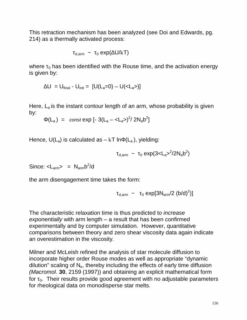
This retraction mechanism has been analyzed (see Doi and Edwards, pg. 214) as a thermally activated process: τd,arm ~ τ0 exp(∆U/kT) where τ0 has been identified with the Rouse time, and the activation energy is given by: ∆U = Ufinal - Uinit = [U(La=0) – U(<La>)] Here, La is the instant contour length of an arm, whose probability is given by: Φ(La ) = const exp [- 3(La – <La>)2/ 2Nab2] Hence, U(La) is calculated as – kT lnΦ(La ), yielding:

τd,arm ~ τ0 exp(3<La>2/2Nab2) Since: <Larm> = Narmb2/d the arm disengagement time takes the form:

τd,arm ~ τ0 exp[3Narm/2 (b/d)2)] The characteristic relaxation time is thus predicted to increase exponentially with arm length – a result that has been confirmed experimentally and by computer simulation. However, quantitative comparisons between theory and zero shear viscosity data again indicate an overestimation in the viscosity. Milner and McLeish refined the analysis of star molecule diffusion to incorporate higher order Rouse modes as well as appropriate “dynamic dilution” scaling of Ne, thereby including the effects of early time diffusion (Macromol. 30, 2159 (1997)) and obtaining an explicit mathematical form for τ0. Their results provide good agreement with no adjustable parameters for rheological data on monodisperse star melts.

151

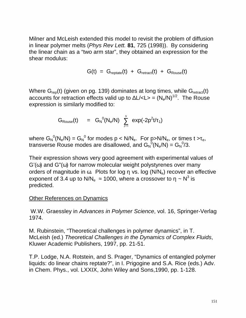
Milner and McLeish extended this model to revisit the problem of diffusion in linear polymer melts (Phys Rev Lett. 81, 725 (1998)). By considering the linear chain as a “two arm star”, they obtained an expression for the shear modulus:

G(t) = Greptate(t) + Gretract(t) + GRouse(t) Where Grep(t) (given on pg. 139) dominates at long times, while Gretract(t) accounts for retraction effects valid up to ∆L/<L> = (Ne/N)1/2. The Rouse expression is similarly modified to: GRouse(t) = GN

0(Ne/N) ∑=

N

p 1exp(-2p2t/τ1)

where GN

0(Ne/N) = GN0 for modes p < N/Ne. For p>N/Ne, or times t >τe,

transverse Rouse modes are disallowed, and GN0(Ne/N) = GN

0/3. Their expression shows very good agreement with experimental values of G’(ω) and G”(ω) for narrow molecular weight polystyrenes over many orders of magnitude in ω. Plots for log η vs. log (N/Ne) recover an effective exponent of 3.4 up to N/Ne ≈ 1000, where a crossover to η ~ N3 is predicted. Other References on Dynamics W.W. Graessley in Advances in Polymer Science, vol. 16, Springer-Verlag 1974. M. Rubinstein, “Theoretical challenges in polymer dynamics”, in T. McLeish (ed.) Theoretical Challenges in the Dynamics of Complex Fluids, Kluwer Academic Publishers, 1997, pp. 21-51. T.P. Lodge, N.A. Rotstein, and S. Prager, “Dynamics of entangled polymer liquids: do linear chains reptate?”, in I. Prigogine and S.A. Rice (eds.) Adv. in Chem. Phys., vol. LXXIX, John Wiley and Sons,1990, pp. 1-128.