Embed Size (px)
Citation preview

Politics of Income Inequality and Government Redistributive Policies
By
Dong-wook Lee
A dissertation submitted to the faculty of Claremont Graduate
University in partial fulfillment of the requirements for the degree
of Doctor of Philosophy in Political Science
Claremont, California
2016
© Copyright by Dong-wook Lee, 2016
All rights reserved.
APPROVAL OF THE DISSERTATION COMMITTEE
This dissertation has been duly read, reviewed, and critiqued by the Committee listed below,
which hereby approves the manuscript of Dong-wook Lee as fulfilling the scope and quality
requirements for meriting the degree of Doctor of Philosophy in Political Science.
Dr. Eunyoung Ha, Chair
Claremont Graduate University
Assistant Professor of Political Science
Dr. Melissa Rogers
Claremont Graduate University
Assistant Professor of Political Science
Dr. Jennifer Merolla
University of California, Riverside
Professor of Political Science
Dr. Luciana Dar
University of California, Riverside
Assistant Professor of Higher Education

Abstract
Politics of Income Inequality and Government Redistributive Policies
by
Dong-wook Lee
Claremont Graduate University: 2016
This study examines why redistributive conflicts are high among countries with
economically diverse regions, and how these conflicts shape the way tax-funded public money is
spent on different public programs. I answer these questions in three steps: 1) civic preferences
for redistribution are formed locally, depending on the geographic regions where people live; 2)
in a decentralized nation with economically disparate regions, this geographic pattern escalates
regional conflicts over redistributive policies broadly consumed by the entire society, such as
public education spending; 3) policy compromises under conditions of inter-regional
redistributive conflicts may result in redistributive policies that are more targeted towards
benefits for specific individuals across the country, such as social welfare.
On each of these steps, I provide supporting empirical evidence. First, drawing the most
recent public opinion data from the Korean General Social Survey on the citizen’s support for
the increased centralized redistribution of public education spending, I find evidence that
residents in poorer regions are more supportive of increased public education spending whereas
residents in richer regions are less favorable. Second, to test cross-national variations in
redistributive conflicts among economically disparate regions with policy autonomy, I use a new

measure of economic disparities among regions that capture a cross-nationally comparable intra-
country income variance. When testing the joint effect of severity of economic disparities among
regions and strength of regional autonomy on volatility in public education spending across
OECD countries from 1980 to 2010, I find that this combined condition reduces the volatility. It
is suggested that the joint condition makes it harder to deviate from the status quo spending,
leading to policy gridlock. Third, when looking at the OECD data on social welfare spending
(excluding education spending) which is directed to individualistic benefits, economic disparities
among regions interacts with regional autonomy to affect more positive changes in social
spending. This result is robust when applying an alternative measure of policy commitment to
targeted spending that considers the government’s policy priorities over competing for budget
allocation categories.
Overall, this research suggests that the joint condition of severity in economic disparities
among regions and strength in regional autonomy exacerbates inter-regional conflicts over the
centralized redistribution of public spending where benefits are broadly consumed but remain
geographically isolated. However, through the targeted spending programs where profits are
directed to specific individuals regardless of their residential regions, autonomous regions with a
different distribution of income improve on coordination to facilitate the centralized
redistribution of public spending.

v
TABLE OF CONTENTS
CHAPTER 1: INTRODUCTION ………………………………………………..…………
A Puzzle on the Inter-personal Income Inequality-Public Spending Nexus …….…..
Research Extension: The Uneven Economic Geography of Income Distribution …..
Redistributive Conflicts: Why Regional Disparity and Regional Autonomy
Jointly Matters ..........................................……………………………………………
Redistributive Conflicts and Strategic Policy Choices ...…………………………….
The Organization of Arguments and Evidence …….………………………...………
1
2
8
8
11
12
CHAPTER 2: THEORETICAL FRAMEWORK (POLITICS OF INCOME
INEQUALITY AND REDISTRIBUTIVE ONFLICTS) ...………………………….……..
Regional Disparities and Individual Redistributive Motives ………………………..
Inter-regional Disparity, Regional Autonomy, and Broad Redistributive Spending ...
Inter-personal Income Disparity with a Unitary System of Government ……
Inter-personal Income Disparity with Federalism ……………………………….
Inter-regional Income Disparity with a Unitary System of Government ………..
Inter-regional Income Disparity with Federalism ……………………………….
Policy Targeting: Preference Convergence among Disparate Regions with Policy
Autonomy ……………………….…………………………………………………...
18
18
22
26
27
30
31
34
CHAPTER 3: SPATIAL PATTERNS OF INDIVIDUAL SUPPORT FOR PUBLIC
EDUCATION FINANCING (EVIDENCE FROM SOUTH KOREA) …………….………..
Case Selection: The Structure of Public Education Financing in South Korea ……...
39
40

vi
Theoretical Frame: Individual Income Positions and Preferences for Public
Education Subsidies …………………………………………………………………..
Survey Data for Empirical Validation ………………………………………………..
Dependent Variable …………………………………………………………………..
Independent Variables ………………………………………………………………..
Distribution of National Wealth across Regions ………………………………....
Distribution of Individual Incomes ……………………………………………....
Controls ………………………………………………………………………………
Model Specification and Estimation Strategy ………………………………………..
Empirical Results …………………..………………………………………………...
Model Fit ……………………………………………………………………………...
Robustness Tests …………………………………………………………………...…
Conclusions and Policy Implications ………………………………………………....
43
45
50
51
51
53
60
63
65
71
72
76
CHAPTER 4: COUNTRY-LEVEL APPLICATION TO COMPARATIVE PUBLIC
POLICIES (FEDERLISM, REGIONAL INEQUALITY, AND EDUCATION
SPENDING) ……………………………………………………………….............................
Governing Structure Matters: Politics of Income Inequality on the
Redistribution of Public Education Spending ………………………………………...
Data …………………………………………………………………………………...
Dependent Variable …………………………………………………………………..
Measures of Inter-personal Inequality ………………………………………………..
Measures of Inter-regional Inequality………………………………………………...
80
82
84
85
85
87

vii
Two Uncorrelated Measures of Inequality …………………………………………...
Measures of Federalism ………………………………………………………………
Controls …………………………………………………………………..…………..
Models, Methods, & Empirical Findings ……………………………………………..
Conclusions and Policy Implications …………………………………….…………...
89
92
94
95
106
CHAPTER 5: EMPIRICAL ANALYSIS OF POLICY BARGAINING (TESTING
THE CONDITIONAL THEORY OF REGIONAL INEQUALITY AND
ECENTRALIZATION) ………………………………………………………………………
Bargaining for a Centralized Provision of Public Policies …………………………...
Data and Methodology ……………………………………………………………….
Statistical Model Specifications ..…………………………………………………….
Dependent Variables …………………………………………..……………………...
Independent Variables ………………………………………………………………..
Controls ……………………………………………………………………………….
Empirical Results …………………..………………………………………………...
Robustness Checks …………………………………………………………………...
Conclusions and Policy Implications …………………………………………………
110
111
115
116
117
126
128
130
138
140
CHAPTER 6: CONCLUDING COMMENTS AND THE CONTRIBUTION OF
RESEARCH TO POLICY GOALS …………………………………………..……………..
REFERENCES ……………………………………………………………………………..
APPENDICES ………………………………………………………………………………
143
147
164

viii
LIST OF TABLES
Table 1.
Patterns of Individuals’ Policy Preferences for Broad Redistribution Explained by the
Uneven Economic Geography of Income Inequality ……………………………………
19
Table 2.
Joint Effects of Economic Disparity and Federalism on Broad
Redistributive Spending ………………………………………………………………...
26
Table 3.
Summary of Household Income Distribution by Regions.…………………..................
54
Table 4.
Summary of Expectations on Support for Increased Education Spending …...................
57
Table 5.
Impact of Household Income Distribution on Public Support for Education
Financing in Korea ……………………………………………………………….…….
66
Table 6.
Marginal Effects of Income Distribution on Public Support for Education Financing …
69
Table 7.
Education Spending and Structure of Inequality in 18 OECD Countries ……………….
86
Table 8.
Inter-regional Inequality and Inter-personal Inequality Compared ….………………….
90
Table 9.
Measures of Federalism …….………………………………………………....................
93
Table 10.
Impacts of Inequality on the Size of Public Education Spending ….……………………
97
Table 11.
Effects of Inter-personal Inequality & Federalism on Public Education Spending ……...
100
Table 12.
Effects of Economic Inequality & Federalism on Volatility of Public Education
Spending ………………………………………………………….……………………...
104
Table 13.
Determinants of Change in Social Expenditure from 1980 to 2010 ..................................
131
Table 14.
Determinants of Change in Policy Priority from 1990 to 2010 ……….…………………
135

ix
LIST OF FIGURES
Figure 1.
Income Inequality and Public Education Spending Compared ………….……………..
7
Figure 2.
U.S. States by Gini Coefficients of Individual Income Inequality ………..……............
30
Figure 3.
Policy Effects of Rising Economic Disparities among Autonomous Regions ………...
37
Figure 4.
Centralized Structure of Education Financing in Korea ………………………………..
41
Figure 5.
Variations in Public Support for Education Financing……………….....………………
47
Figure 6.
Geographic Distribution of Public Support for Education Financing ….....…...………..
49
Figure 7.
The Correlation of Inter-personal Inequality and Inter-regional Inequality ……………
91
Figure 8.
Marginal Effect of Inter-personal Inequality on Public Education Spending,
Conditional on Electoral Federalism ……………………………..…………………….
101
Figure 9.
Marginal Effect of Inter-regional Inequality on Volatility of Public Education
Spending, Conditional on Electoral Federalism ……...………………………………...
105
Figure 10.
Volatility of Social Expenditure across OECD Countries ………………………...……
118
Figure 11.
An OECD Spending Data Replication for Unfolding Analysis ………………….…….
125
Figure 12.
Marginal Effects of Interaction Terms on Changes in Social Expenditure ……………..
133
Figure 13.
Marginal Effects of Interaction Terms on Change in Policy Priority ..………………….
136

1
CHAPTER 1
Introduction
Why do economic disparities among geographic regions within a decentralized country
exacerbate inter-regional conflicts over the centralized redistribution of public spending? More
specifically, how can the severity of regional inequality and the strength of regional policy
autonomy jointly determine a pattern of inter-regional redistributive conflicts? Most
importantly, to what extent does this conditional effect vary by type of redistributive spending
which ranges from the policy benefits broadly consumed by the entire society to the policy
benefits targeted at specific individuals?
To answer these questions, this research first distinguishes inter-regional income
disparity from inter-personal income disparity. Inter-regional income disparity is defined as
inter-regional inequality in regional wealth determined by the income distribution of residents,
while inter-personal income inequality is defined as inter-personal inequality in the nationally
aggregated individual income distribution. This distinction is useful because inter-regional
income disparity better captures redistributive conflicts at the national legislature of regional
representatives. While this is often neglected from a policy perspective, inter-personal income
disparity overly addresses the policy directorship of the poor majority. Furthermore, this
distinction is even more useful when thinking regarding how regional autonomy as an
institutional rule intervenes to mediate redistributive conflicts.
The crux of my argument is that regions diverge in their policy interests against the
centralized redistribution of public spending as inter-regional income disparity becomes severe
and regional autonomy grows stronger while those regional interests collectively shape the

2
residents’ preferences for redistributive policies which are centrally administrated. The likely
policy outcome on broad redistribution is the perpetuation of redistributive conflicts, leading to
the potential for policy gridlock. I also argue for targeted spending where benefits are directed
to individuals across regions as constituting a policy compromise among economically disparate
regions with policy autonomy.
This research contributes to the inequality government spending literature by identifying
an institutional condition under which regional disparity leads to either the perpetuation of a
redistributive conflict or the promotion of a policy compromise, contingent upon how the tax-
funded money is spent.
A Puzzle on the Inter-personal Income Inequality-Public Spending Nexus
Inter-personal income inequality, also known as disparities in the distribution of income
amongst individuals, is an important policy concern in a redistributive government. It matters for
government spending. The literature has determined that inter-personal income inequality harms
economic growth (Easterly, 2007; Berg & Ostry, 2011). Empirical studies demonstrate that inter-
personal income inequality affects economic growth negatively through constraints on human
capital accumulation (Alesina & Rodrik, 1991) or occupational choices (Persson & Tabellini,
1994). Inter-personal income inequality, as noted by Berg and Ostry (2011), may reflect “poor
people’s lack of access to financial services, which gives them fewer opportunities to invest in
education and entrepreneurial activity” (p.34). Governments care about the rise of inter-personal
income inequality because inequality makes it harder for them to make necessary, decisions
during economic hardship such as raising taxes and cutting public spending to avoid a debt crisis.
Moreover, there may be a social backlash against government policies negligent of interpersonal

3
income inequality. Public dissatisfaction can lead to political instability, similar to what was seen
in Greece due to the policy choices of the Greek government in 2011. Unfortunately, political
instability discourages economic investment because a higher likelihood of government collapse
increases economic actors’ uncertainties associated with the return on investment (Alesina &
Perotti, 1996; Goodrich, 1992; De Mesquita & Root, 2000).
The standard theory of redistributive politics proposed by Romer (1975) and expanded by
Meltzer and Richard (1981) is an ideal initial reference point. According to their observations,
the average income of most societies lies above the median income. In a more (right) skewed
distribution of income, median income is lower than median income. Thus, median income
voters are expected to exert political pressures for redistributive government intervention.1 The
benefit that median income voters receive from redistributive interpersonal transfers will be
greater than the costs they pay in taxes needed to finance redistribution.2 The essence of their
model suggests that more redistributive governments are anticipated when the income of the
median (decisive) voters decreases, compared to the average income.
The Romer-Meltzer-Richard (RMR) model, in its application for public spending,
predicts more redistributive spending likely to be found in a society with higher income
inequality. However, how to apply this simple theoretical prediction in an empirical analysis is
1 Based on their numerical advantage in the voting booth, the poor are assumed the winners in this distributional
struggle as increasing inequality pushes the median voter toward the lower end of the income spectrum (Romer,
1975; Meltzer & Richard 1981). Poor individuals may capture legislative majorities to proactively advance
redistribution as interpersonal inequality grows.
2 Two assumptions need to be held: 1) median voters are accounted for political process under majority voting, 2)
taxations should be progressive.

4
less clear. For example, public education spending is one form of government transfer of funds
which helps human capital accumulation. It is often considered more of a “collective good” in
comparison with other government spending categories which are considered more
“individualistic benefits” such as healthcare and social welfare (Jacoby & Schneider, 2009;
Volden & Wiseman, 2007).
One possible explanation why this may be that public education is a policy area in which
benefits are more broadly consumed by the general population rather than being directed to more
specific (especially poor) segments of the population. Indeed, education policy appears to be
more like “collective goods” policies than “particularized goods” often associated with
redistribution. This comparison is empirically demonstrated by Jacoby and Schneider (2009),
who developed a measure of relative policy priorities using yearly data of US state government
finances (1982-2005) in nine policy areas including education, health, and welfare. They found
that education spending was statistically grouped with other collective goods, such as defense
and infrastructure spending and not strongly associated with health and social welfare spending.
General public education (especially non-tertiary) spending is considered a redistributive
policy. The poor individual income earners can benefit more from public education spending
compared to the rich, when sharing (progressive) income tax costs to fund this public provision.
As predicted by the RMR model, an income distribution that is skewed to the right will create
demands for more redistribution of public education spending. In general, the government will
comply to win the median voter’s vote.3 Thus, the impact of individual income inequality on
public education spending is expected to be positive. Using the U.S. government spending data
from 1936 to 1972, Meltzer and Richard (1983) find that the level of government spending,
3 Note that it really depends on the electoral system.

5
including public education, rises with the ratio of mean to median income. Their findings also
suggest that the relative position of the decisive (median) voters in the income distribution is a
more important determinant for redistribution than the level of the individual income. Corcoran
and Evans (2010) present a similar result using the panel data for the U.S. which is constructed
from state and school district spending from 1970 to 2000. They show that growth in inter-
personal income inequality reduces a median voter’s tax share as the burden of progressive tax
rates is imposed on wealthy voters. This reduction induces higher local education spending
because it is more demanded by the median voters.
Although the RMR model has been popularly cited in the government spending literature,
its empirical findings are rather ambiguous. The recent empirical literature indicates that inter-
personal income inequality is negatively associated with a level of redistribution and support for
public services across countries or within the subnational jurisdiction (Glodin & Katz, 1997;
Lindert 1996; Perotti, 1996). The most criticism raised by these empirical works is the difficulty
in applying the RMR model’s assumption about the median income voters. The median income
voters are the crucial voters in a majority rule voting system where a progressive income tax
finances the public provision. However, the decisive voters may be different from the median
voters (Epple & Romano, 1996; Benabou, 2000).
For example, the crucial voters can be determined by a majority voting status defined as
the coalitions of the lower income voters and the upper-income voters against the middle-income
voters (Epple & Romano, 1996; Ansell, 2008a/b). In the domain of public education where
funding requires tax increases and where private options exist, the lower and upper-income
voters might prefer a lower level of public education spending, compared with the middle-
income voters’ preference. The reasons are as follows: 1) the lower income voters favor lower

6
taxes and a greater level of consumption, 2) the higher income voters can opt out for private
education. As income inequality rises, these two opposing groups are more likely to form a
coalition to vote against the middle-income voters. This “ends against the middle” hypothesis
expects a majority voting equilibrium in a lower level of public education expenditures (Ansell
2010). Through a somewhat different mechanism, Goldin and Katz (1997) show supporting
evidence from US data that heterogeneous communities in income distribution were more likely
to lag behind in funding secondary public education, compared to homogenous communities.
Other empirical studies find no statistically significant relationship between inter-
personal income inequality and public education spending. As put forth by Perotti (1992), no
statistically significant association is found because growth-oriented public policy incentives
create more demands for increased public education spending whereas tax burden pressures
dampen those public policy incentives. Moreover, Basset et al. (1999) find that the impact of
inter-personal income inequality on redistributive policies depends on how accurately the
unequal distribution of individual income represent the position of median income voters. Also,
aggregated public education expenditures are often considered too broad to be used as outcomes
to be explained by individual income inequality. As indicated by Zhang (2002), the sectoral
education expenditure may differ by how socio-economic classes interact with the policy process
to affect the allocation of public spending across education levels.
Figure 1 presents time series observations of public education spending for 18 OECD
countries with regards to their Gini index level, a scale of inequality in the nationally aggregated
individual income distribution. A higher level of Gini (as expressed on a scale of 0-100)
indicates more unequal income distributions. The different country plots are shown in Figure 1.
They include overall public education spending as a share of GDP. As illustrated in Figure 1,

7
Figure 1. Income Inequality and Public Education Spending Compared
Data sources: GINI index is based on market (pre-transfer & pre-tax) income. The index value can go from 0 to 100,
where zero is perfect equality. This GINI index is available from the Standardized World Income Inequality
Database (http://myweb.uiowa.edu/fsolt/swiid/swiid.html); Public education spending data is measured as % of
GDP. The dataset is available from World Development Indicators, World Bank.
variations in public education spending across countries over time do not necessarily correspond
with the RMR model prediction: in other words, a higher level of Gini will coincide with the
expansion of public education spending. In contrast with this theoretical expectation, we find that
countries’ education spending patterns vary considerably. For example, Denmark and Finland
roughly match with the RMR prediction, but Canada and Ireland clearly do not. The RMR model
prediction applied to public education spending is unclear empirically. Why would a country
reduce education spending while its inequality continues to rise? This empirical puzzle is not

8
addressed by the RMR model assumption. In the following section, I will discuss how the study
of inequality types helps improve our understanding of variations in public education spending.
Research Extension: The Uneven Economic Geography of Income Distribution
The RMR model of public expenditures assumes that the national median voters decide
the redistributive policy during a national referendum process. However, this assumption
overlooks the fact that individual citizens and policymaking power are geographically spread
across subnational regions, and peoples’ votes are usually represented based on a geographical
unit (i.e. political jurisdictions such as states in the U.S., cantons in Switzerland, or provinces in
Canada) even at the national level. Each region has different income characteristics, reflecting
both the income level and the income distribution. The national median income is not necessarily
identical to the median income of a region. These regional differences may result in different
preferences for national policy. Accordingly, the heterogeneity of median voters’ policy interests
should increase with the rise of inter-regional inequality, defined as differences in regional
incomes within the nation.4
Redistributive Conflicts: Why Regional Disparity and Regional Autonomy Jointly Matters
The concept of inter-regional income disparities is a useful one. It helps us better
understand individual redistributive interests subject to the uneven economic geography of the
4 Many works, among the RMR modelers, rely on an implicit assumption that inter-personal income disparity
captures inter-regional inequality, and typically ignore inter-regional inequality altogether. A growing number of
studies on inter-regional inequality has recognized conceptual differences in inequality of both types (Beramendi,
2012; Giuranno, 2009a/b).

9
income distribution. Similar to the logic of redistributive policies at the individual level,
wealthier regions have the larger fiscal burdens to finance the centralized redistribution in a
progressive tax system. Where regional policy autonomy is possible, it may be in the best
interest of citizens of affluent regions to seek redistribution within their jurisdictions rather than
centralized redistribution. Isolating public financing and redistribution within a region allow for
reducing the relative cost incurred by wealthy citizens in rich regions. For poor citizens in rich
regions, keeping the local revenue and expenditure inside their regional territory serves to secure
more redistributive benefits available to them. Conversely, wealthy citizens and poor citizens are
similar in less affluent regions. They prefer the centralized redistribution of public spending to
less, and more so as regional disparity increases. The reason for this public choice is that the
centralized redistribution brings more benefits to poor citizens and wealthy citizens in the poor
regions which are subsidized by their counterparts in affluent regions.
Because geographical interests shape individual redistributive interests, inter-regional
inequality creates tensions between equity and efficiency regarding the redistribution of public
goods, including education spending. A government may introduce a redistributive mechanism
to financing public goods to reach the targeted equity. A government function lies in transferring
income from richer regions to less affluent regions, through broad uniform provisions of public
goods and services (Tanzi, 2000). Although the vast redistribution helps gains in equity, it can
also come with a loss of efficiency. It is less efficient for the regions with higher GDP per capita
income to share public resources with their poor regional counterparts, despite the fact that
sharing improves equity for poorer regions. Thus, inter-regional asymmetry in wealth can create
losers (the richer regions) and winners (the poorer regions) regarding government interventions

10
(Decressin, 2002). Therefore, the more affluent regions are less incentivized than their poorer
regional counterparts to support the centralized system of uniform redistribution.
A few empirical studies have indeed confirmed the dampening effects of inter-regional
inequality on the size of public education spending (Decressin, 2002; Sibiano & Agasisti, 2012).
The Italian case is noteworthy. Italy has a centralized system of uniform redistribution regarding
public education spending. The country targets equity across its subnational regions with very
high economic gaps (Barro & Sala-I-Martin, 2004). Regions in Italy have some ability to set the
tax rates for local revenues. Using public spending outcomes (the students’ performance in
national test scores by 18 Italian regions), Sibiano and Agasisti (2012) conclude that rich regions
tend to find the uniform redistribution of education spending across the whole nation less
efficient and poor regions find it more efficient regarding the students’ academic performance.
The rise of inter-regional disparity allows losers and winners of redistribution to be more easily
identified. This disparity can undermine support for redistributive policies. In a cross-national
comparison, this reduction is illustrated by Decressin’s (2002) empirical findings: Italy is less
redistributive in public education spending than other European countries such as France and the
United Kingdom, where a lower level of inter-regional inequality is reported. The reason for
drastically less redistribution in Italy is that rich regions have become less supportive of
redistribution due to their low elasticity of education outcomes on taxes paid (Giorno et al.,
1995).
While there is a redistributive policy tension between rich regions and poor regions, a
system that grants regions policy autonomy and thus increases the bargaining power of regions,
intervenes to aggravate (or perpetuate) the redistributive conflicts between rich regions and poor
regions. Several studies on redistributive politics emphasize the causal role of regional
11
autonomy (e.g., Cameron, 1978; Weingast et al., 1981; Cox, 2001; Besley & Coate, 2003;
Lessmann, 2009). However, their focus only hints at the importance of an institutional context
in which inequality plays a role in shaping the redistribution of public education spending.
The problem is that neglecting regional inequality can lead to very different policy
predictions about the conditional effects of regional autonomy on public spending outcomes.
For instance, regional autonomy (whether it is political or fiscal) is based upon the
constitutional rule of sharing national policymaking power by subnational regions. Regional
autonomy allows for multiple institutional channels for public policy access. Among
economically homogenous regions (as small replicas of the RMR polity with a high inter-
personal income disparity), regional autonomy becomes an institutional vehicle of deficit
spending on public education. While the attached cost is equally shared by autonomous regions,
the cost becomes relatively smaller than the policy benefit to each region as regional autonomy
increases (see, the fractionalization of national decision making explained by Franzese 2005).
On the other hand, when regional inequality accounts for the conditional effect of
regional autonomy, one should be concerned about polarization in policy preferences of unequal
regions, especially as inter-regional disparity increases. In this case, regional autonomy
becomes a system of regional representation which exacerbates the redistributive conflicts
among economically uneven regions, leading to the perpetuation of the status quo spending.
This comparative example suggests that neglecting regional inequality leads to an incomplete
picture of policy outputs across nations.
Redistributive Conflicts and Strategic Policy Choices

12
The regional autonomy mechanism that makes it difficult to draw a policy compromise
among disparate regions may work in the opposite way, depending on how public money is
spent. While regions may not be able to agree on policies that are explicitly redistributive to poor
regions, they may be able to compromise on policies that benefit large segments of all regions.
There are three noteworthy conditions in which individually-targeted policies such as social
welfare may benefit rich regions: 1) if they reduce the possibility of large population migrations
away from the poor regions; 2) if they compensate for job market risks which are present in the
rich regions; and 3) if rich regions have high levels of inequality.
California, for example, has strong interests in centralized redistribution, despite being a
rich region, for all three reasons just described. California’s welfare policies and job market
opportunities may bring too many immigrants to the state if central welfare systems are not
generous for people to remain in poorer regions. Job market risks are acute in California,
including high-income professions like the technology sector, which increases demand for
unemployment insurance and stable healthcare access. Moreover, California is one of the most
unequal states regarding income strata, meaning that they have a lot of needy individuals who
would benefit from central redistributive policies.
Likewise, poor citizens in rich regions find this individually targeted spending to their
advantage while it also spillovers policy benefits to qualified individuals in poor regions.
Targeted spending is this region’s strategic choice subject to bargaining over competitive policy
programs. It attenuates redistributive conflicts among disparate regions.
The Organization of Arguments and Evidence

13
The road map of overall theoretical exposition and empirical falsification is organized as
follows. Chapter 2 theorizes how individuals’ policy preferences are collectively shaped,
depending on whether they live in rich or poor regions and the targeting of the policy area. I
show a simple utility model to demonstrate benefits and costs of supporting cross-regional
redistribution by individual citizens who are geographically spread in economically disparate
regions. My assumption is that all citizens seek to maximize their benefits from distributive
policies by sharing the associated costs. I apply this assumption to policy motivations of both
poor and rich individuals in affluent regions, predicting that higher regional disparity in wealth
incurs more costs than benefits from the centralized redistribution of public goods and services.
Thus, I anticipate that those residents of affluent regions are less likely to support increases in
centralized redistribution with the rise of regional disparity. I also elaborate the opposite policy
expectation for redistributive motives of both poor and rich individuals in less affluent regions. I
explain that their relative gains from supporting centralized redistribution increase with the rise
of regional inequality.
Extending from the micro-foundations of redistributive motives among individuals
within a country, I explore macro-level variations in policy outcomes across countries. I analyze
whether decentralization (regional autonomy) may interact with rising regional inequality to
affect policy outcomes. I argue that the wealthy regions with more policy-making autonomy will
be more capable of constraining government distributive policies despite most less affluent
citizens with an interest in redistributing wealth. On the other hand, these less affluent regions
are likely to try to block the rich regions’ efforts to reduce redistributive spending. Thus, my
expectation is that countries with more decentralized systems of governance and higher levels of

14
regional inequality are likely to show policy gridlock, leading to less change in centralized
redistributive spending for the broader benefits of the entire society.
Due to this policy gridlock, however, I also anticipate more compromise between the
rich and the poor regions for centralized legislation over policies that target direct benefits
towards segments of the population across all jurisdictions. This targeted policy spending in the
poor regions will be beneficial because it meets large demands from local constituencies. This
benefits the rich regions also because targeted spending helps their local constituencies who rely
on welfare provision. This common interest will make policy bargaining easier, leading to
increases in redistributive spending on targeted policies for individualistic goods.
In Chapter 3, I test the empirical merits of my argument that regional interests trump (or
interact with) individual redistributive motives. I use the individual-level data from the Korean
General Social Survey (2006) on citizen support for increases in public education spending.
The Korean case is interesting because regional political autonomy has grown stronger in
recent years while income tax systems for financing public education have long been centrally
administrated. To explain variations in citizen support for Korean education spending, I probe
models of cross-level interactions between income attributes of individuals and economic
disparities in regions where those individuals are geographically dispersed. My empirical
analyses yield a finding that both rich and poor residents of rich regions in general have a weak
incentive to support more tax-funded spending on public education, whereas those of poor
regions have a strong incentive to support increases in funding for public education spending.
This finding implies that in centralized broad redistributive programs such as public education,
regional disparity makes the difference in the policy incentive between net benefactors from
poor regions and net contributors from rich regions more visible. Thus, the redistributive

15
policies preferred by economically disparate regions are difficult to coordinate at the national
level.
Moving from a single survey data analysis to cross-national statistics mainly focused on
advanced economies, Chapter 4 tests cross-national differences in policy rigidity explained by a
country’s degree of economic disparity among autonomous subnational regions. In a policy
bargaining, collective regional interests exacerbate redistributive conflicts as regional income
grows more disparate and regions have more power to influence national policy making. I
predict that disparity in regional income increases heterogeneous preferences, thus creating
barriers to national policy reform. For data analyses, I use a new dataset for inter-regional
inequality measured by regional GDP per capita. The database measures inter-regional inequality
in two ways: 1) the dispersion of regional wealth, weighted by each region’s relative size to the
population; 2) the structure of regional wealth distribution, weighted by the relatively deprivation
of each region. Both inter-regional inequality measures are cross-nationally comparable variables
of intra-country variance. Then I test how inter-regional inequality interacts with regional
autonomy (measured in degree of electoral or fiscal federalism) to affect redistributive spending.
Using panel data covering 18 OECD countries from 1980-2010, I confirm that inter-regional
inequality interacts with federalism to exacerbate policy impasses, driving down changes in
public education spending.
In contrast to rigidity in education financing, broadly consumed by general population
across disparate regions in regionally autonomous nations, Chapter 5 provides an empirical
assessment of flexibility in financing public programs that are directed to specific individuals
regardless of region. I predict that if policy benefits are more targeted to demographic segments
of the population (e.g., welfare spending and Medicare), policy concessions on national

16
legislation will be easier because this targeted policy provision brings particularized benefits to
constituency needs for public goods and services -- common demands from every local region.
In this regard, my empirical test focuses on the join impacts of economic disparities and
decentralized authority structures among subnational regions on changes in targeted public
spending. Using the cross-national data on social spending in 24 OECD countries from 1980-
2010, I find evidence that higher inter-regional inequality in a more decentralized polity leads to
more growth on social expenditure. More importantly, considering trade-offs between spending
allocation across policy areas, I examine the relative importance of social spending to other
policy goods broadly consumed by nontargeted general population (e.g., national defense, public
order and security). The associated finding also reveals that countries with more disparate
regions and decentralized authority structures tend to prioritize social spending over other
nontargeted spending policies. This suggests that not all types of public programs preferred by
the disparate regions with strong local autonomies necessarily lead to a policy impasse. Instead,
depending on where and for whom to target, conflicts of the redistributive interests can lead to
more compromise on certain programs than others.
Chapter 6 presents a conclusion with policy implications. In short, the understanding of
geographic-based inequality that I employ provides a more detailed explanation of policy
behavior of individuals than the national-level income strata modeling extensively used in the
existing literature. My research further distinguishes itself by identifying political
decentralization as a relevant institutional factor in an overall explanatory framework because
it amplifies the effect of inter-regional inequality on preferences for government redistribution.
This analytic frame can be applied to a wide range of topics from government finances and
public choices in general to legislative conflicts. It can be also used as a reference to integrated

17
research between individuals within regions within countries. Moreover, my findings strongly
suggest that countries may be able to achieve redistributive spending in some policy areas
more effectively than in others, given the nature of their region-specific income inequality and
institution structures.

18
CHAPTER 2
Theoretical Framework: Politics of Income Inequality and Redistributive Conflicts
The primary goal of this theoretical chapter is to identify how inter-regional income
disparity and regional autonomy jointly constrain the centralized redistribution of public
spending whose policy benefits are broadly consumed by the society but often geographically
isolated (e.g., public education spending). A negative social outcome is anticipated as a result of
policy conflicts among disparate regions over the centralized redistribution of nontargeted
spending. This expectation needs to be separated from a potential for the policy coordination
incentives shared among regions toward targetted spending that directs policy benefits to be
directed to specific (qualified) individuals regardless of their geographic regions (e.g., social
welfare spending). I predict that the former case makes it harder to change the broad
redistributive spending, whereas the latter one induces more positive changes in targeted
redistributive spending. Thus, policy targeting would be an important matter, particularly when
regional disparity grows and regional policy autonomy is stronger.
Regional Disparities and Individual Redistributive Motives
Beramendi (2012) provides a very useful theoretical frame that draws patterns of inter-
personal redistribution based on economic geography. This frame predicts a wider gap in
preferences for inter-personal redistribution across economically disparate regions. A predictable
policy outcome, according to Beramendi (2012), is regional governments’ design of policies for
redistribution among citizens within their territorial units, without extensively resorting to either
interregional transfers or central government coordination.

19
Table 1. Patterns of Individuals’ Policy Preferences for Broad Redistribution
Explained by the Uneven Economic Geography of Income Inequality
Poorer Regions Richer Regions
Poorer Residents More Support Less Support*
Richer Residents More Support* Less Support
Note * Individual residents experience a policy preference dilemma where the political geography trumps class-
interests. This theoretical framework is first introduced by Beramendi (2012). In this civic preference model, I
simplify the analytical frame by assuming regions have a certain degree of regional autonomy and the progressive
tax rate on income is uniformly imposed across disparate regions.
I develop a modified version of Beramendi’s (2012) original setup using two-axis of
redistribution: inter-personal redistribution (from rich to poor citizens) vs. inter-regional
redistribution (from rich to poor regions). Importantly, Beramendi (2012) stresses that the fiscal
structure of redistribution (e.g., full centralization, full decentralization, or hybrid) can be an
outcome of elite choice to overcome the uneven economic geography of income inequality.5 My
research differs from Beramendi’s (2012) by focusing on the role of regional autonomy together
with inter-regional income disparity as a process which determines redistributive spending. I
examine how the uneven economic geography of income distribution in autonomous regions
(wherein the regional government can limit inter-regional redistribution) affects individual
preferences for policy goods broadly redistributed.
The distribution of individual income falls into four groups whose preferences reflect the
underlying geography of inequality. As shown in Table 1, there are four distinctive individual
groups: poorer residents in poorer regions, richer residents in poorer regions, poorer residents in
richer regions, and richer residents in richer regions. First, richer residents in richer regions have
5 Beramendi also looks at other conditions such as regional economic specialization, cross-regional labor mobility,
and the configuration of (centripetal and centrifugal) political representation.

20
no incentive to agree to any transfer of their tax bases towards redistributive spending which
goes disproportionately to the country’s poorer regions. Therefore, richer residents in richer
regions are less likely to be for the increased centralized redistribution of public spending funded
disproportionally by rich regions.
Second, poorer residents in poorer regions receive the most benefits from centralized
spending distributed inter-regionally and will support its expansion (as disproportionally funded
by rich regions). A full redistribution of public spending will be the best policy option for poorer
residents in poorer regions. Their expectation of the redistribution will be large, seeking to
extract resources from inter-regional transfers out of the base of richer regions.
Third, as with poorer residents in poorer regions, similar logic applies for richer residents
in poorer regions: they are more likely to support the broad redistribution of public spending.
These richer individuals want to pay as few taxes as possible, but at the same time, they want to
extract as many resources from other wealthier regions as possible. This situation creates a
dilemma for richer residents in poorer regions. For the broad redistribution of public spending
within a poorer region, richer residents will pay more taxes than poorer residents. Those richer
residents may not prefer this option. However, when this non-targeted public spending is inter-
regionally redistributed, it could lessen the fiscal burden on richer residents in poorer regions and
improve the economic condition of their poor residents. Thus, richer residents in poorer regions
are more likely to support the broad national redistribution of public spending.
Fourth, poorer residents in richer regions will not agree with inter-regional transfers of
public spending because they lose more than what they would gain through intra-regional
transfers. They also experience a policy preference dilemma although this experience differs in
nature from what richer residents in poorer regions would experience. One the one hand, poorer

21
residents in richer regions can extract additional resources from the wealthier individuals (in
poorer regions) by supporting the broad redistribution of public spending. On the other hand, this
inter-regional redistribution will require residents in richer regions to share their tax bases with
residents in poorer regions. To poorer residents in richer regions, this means that the costs of
sharing can exceed benefits from it, especially as regions increasingly vary by levels of income.
Since the governing system of regional autonomy allows for the regional government to enact
autonomous policies, poorer residents in richer regions will pursue a decentralized system of
inter-personal redistribution in which they benefit the most from fiscal transfers occurring only
within their region. Therefore, the redistributive motives of poorer residents in richer regions are
less supportive of broad centralized redistribution of public spending.
In short, Table 1 summarizes how the uneven economic geography of the income
distribution would matter and becomes a political problem (Weingast et al., 1981; Rodden, 2000;
Giuranno, 2009a/b). Citizens’ redistributive interests can be collectively formed depending on
the level of regional wealth rather than the level of individual income, especially in a system of
government that grants regional policy autonomy. As pointed by Beramendi (2012), we may not
see the effects of political geography on the redistribution of public education spending when the
relative level of individual income overlaps strongly with the relative level of regional wealth
(poorer residents in poorer regions or richer residents in richer regions). In such places,
redistributive policies follow individual redistributive motives. More redistribution is preferred
by poor citizens to less (vice versa for rich citizens). However, when individual income and
regional wealth are mismatched, political geography matters more (Beramendi 2012). This
relationship occurs because regional incentives can alter individual redistributive motives
(denoted as * in Table 1).

22
This theoretical framework assumes that poorer residents in richer regions and richer
residents in poorer regions do not necessarily follow class-based interest. Rather, the economic
geography trumps their redistributive motives in the case of policy preferences for the
centralized redistribution of public goods broadly redistributed across disparate regions. This
relationship leads to a testable hypothesis as follows.
Hypothesis 1: Poor citizens in rich regions are less likely to favor of the centrally-
managed broad redistributive spending, whereas rich citizens in poor regions tend to be
more in favor.
A broader implication of this individual-level analysis is that regional disparity increases
redistributive policy tension among disparate regions. The structure of political representation
will further mediate this redistributive conflict. The following section applies this for a cross-
national dimension. I expect more severe conflicts among disparate regions where regional
policy autonomy is possible, compared to a unitary system of government.6
Inter-regional Disparity, Regional Autonomy, and Broad Redistributive Spending
6 It is possible that the rich in poor regions might be even richer than the rich in rich regions. Similarly, the poor in
rich regions might be poorer than the poor in poor regions. However, on average, I assume that the poor in poor
regions is a group of the poorest individuals whereas the rich in rich regions is a group of the richest individuals in
their income status nationwide. See Footnote 36 in Chapter 3 with tangible evidence from the Korean General Social
Survey data in 2006.

23
The policy effect of regional autonomy has long been debated in the field. For example,
federalism (as an institutional form of regional autonomy) is a system of government with semi-
autonomous subnational regions in a regime with the common central government (Riker, 1964).
This system allows for local politicians representing subnational governments to cater to local
demands (Bednar, 2011). Policy administration under a federal system can be more efficient to
cope with local demands, compared to a unitary system of government which seeks “one size fits
all policies” for varied regional interests (Tiebout, 1956; Oates, 1972). While federalism
promotes diversity in the ways that local supplies meet local demands, it creates two competing
forces. First, federalism allows local constituencies to have more access to policy processes
through multiple governments; this highlights the fractionalization effects of national policy
making. The second, the competing force arises when the heterogeneity of administrative regions
under federalism also increase constraints on policy agreement among regions at the national
level (Aysan, 2005a/b). As their policy interests diverge, regions can be highly polarized in their
policy ideals regarding national policy-making.7
Not surprisingly, empirical studies of federalism reveal mixed findings of the policy
effects of federalism. Comparative cross-national studies present no clear relationship in policy
outcomes. Some scholars find that federalism leads to more redistribution among developed
countries due to their high fiscal decentralization capacity to either compensate inequality or
deliver public services (Rodríguez-Pose & Ezcurra, 2010; Lessmann, 2009). However, empirical
work of other scholars provides a counterexample where federalism reduces redistribution
because it undermines the power of the central government to play an equalizing role
(Prud’homme, 1995: Rodríguez-Pose & Ezcurra, 2004). Evidence from policies pursued in a
7 I borrowed the following terms “fractionalization effects” and “polarization effects” from Franzese (2005).

24
sample of European regions suggests that federalism disproportionately benefits a few specific
geographic locations (Cheshire & Gordon, 1998).
The existing research, however, fails to explain the separate conditions which distinguish
the effect of federalism engendering the exploitation of the common pool, from that of
federalism increasing policy veto constraints.8 Common pool issues arise when multiple regions
share fiscal policy authority. Local politicians try to please their constituents and attract
taxpayers and, thus, they seek to provide high-quality public services. In policy practice, a
region’s parochial interests will push for more resources while competing with other localities
(Tiebout, 1956; Weingast, 1995). One of the related consequences is that when regions make
decisions in the national legislature together, they often pass oversized budgets (Weingast et al.,
1981). They are likely to remain cooperative in national policy making, benefiting from
logrolling, or “pork-barrel spending proportional to the number of districts,” as put by Franzese
(2005). The problem is then that their benefits from expansionary policies would exceed their
share of the fiscal burden in public financing; especially when the cost accrues more uniformly
across subnational regions (according to the law of 1/n, see Franzese, 2005). Therefore, the more
the political power shared by regional governments, the greater the potential that will be invested
in regional governments to push for the central government to provide what the regional
governments want (Barro & Gordon, 1983; Kydland & Prescott, 1977). This local incentive will
result in the overuse of the common pool of public funds in distributing benefits specific to local
demands (Franzese, 2005). As predicted by Weingast et al. (1981), the division of labor in policy
making by subnational actors will lead to deficit spending on national policies as it makes
8 Franzese (2005) is a complement. At a slightly different angle, my argument focuses on the question of how
inequality measures highlight such distinction in a different way.

25
logrolling more attractive and ensures more uniform sharing of the cost attached to redistributive
spending.
While the common pool effects are derived from the fractionalization of federalism, the
increased veto constraints under federalism can lead to policy impasse (Franzese, 2005). The
number of veto points is created using institutional separation. These veto points become
competitive when separate institutions vary in their policy preference. Federalism is a system
which divides power between many sub-national decision makers rather than focusing on one
single national authority. It diffuses policy decision power through institutional separation where
different political actors compete through those separate institutions with mutual veto powers
(Triesman, 2000; Tsebelis, 2002; Crepaz & Mozar, 2004). As pointed out by Cox (2001),
because more actors are becoming involved in policy decision making under federalism, they are
more capable of blocking decisions.9 Therefore, any dispersion of political authority is expected
to increase the number of veto players, which would perpetuate the status quo (Treisman, 2006).
Moreover, the number of veto points may remain more competitive when regional governments
are polarized in their policy preference. Competitive veto points reduce the bargaining space for
inter-regional policy agreement and incur high transaction costs to policy making (Cameron,
1978; Tsebelis, 1995, 2002; Persson & Tabellini, 2006). For example, Treisman (2000) finds that
federalism blocks policy changes to the money supply. Federalist countries with a high level of
money supplies have kept the supply high, while those with a low level of money supplies have
remained low. Similarly, the competitive veto player constraints can lock in a country’s existing
degree of public spending.
9 The U.S. Senate filibuster would be a good example of delaying the entire legislative process and forcing a
supermajority coalition to override it.

26
Table 2. Joint Effects of Economic Disparity and Federalism
on Broad Redistributive Spending
Inter-personal Disparity Inter-regional Disparity
Unitary Increase or Decrease (A) Change (C)
Federalism Greater Increase (B) Less Change (D)
The conflicting expectations of overdrawing from the common pool and policy
stalemates between competitive vetoes created under federalism can help us identify how these
policy problems have become more severe when thinking regarding inter-personal income
disparity and inter-regional income disparity, more than what we might see in a unitary system of
government. Common pool effects causing the over provision of public spending will rise further
when the interplay between a higher level of inter-personal disparity (translated into smaller
replicas of the nation) and a greater extent of policy access granted by regional autonomy (i.e.,
the fractionalization effects). The delays on policy adjustment incurred by competitive veto
player constraints will become even more intransigent at the interplay between higher levels of
inter-regional inequality and more different policy interests which results from regional
autonomy (i.e. the polarization effects). Details of these interaction effects are organized in
Table 2.
(A) Inter-personal Income Disparity with a Unitary System of Government
In a unitary system of government, all governing authority is vested in a central
government. Although it is possible to have regional autonomy to some extent, sovereign power
rests with the central administration; it will stay supreme. France is an example of a nation

27
having a strong unitary system of government. Although the country has 90 departments and 36
provinces, these provinces do not have the power commonly exercised by states in the U.S.
Inter-personal income disparity of a centralized polity, holding the level of inter-regional
disparity constant, could have more redistribution of public spending. As the median income
decreases relative to the average income, the median income voters will demand increased broad
redistribution in public expenditure. The government will supply more to improve equity in the
entire country. The increase in broad public spending will be reasonable to win the support of the
median income voter. In an ideal RMR world (with progressive taxation and majority voting),
high inter-personal inequality will increase the amount of public spending broadly consumed.
On the other hand, the size of broad public spending could decrease at high levels of
inter-personal income disparity. A higher level of inter-personal disparity will result in the
polarization of individual voters’ (and their representatives’) policy preferences. Political parties
may not be directly responsive to the national median voters (Iversen & Soskie, 2006a/b;
Stratmann, 1995; Gerber & Lewis, 2004). Also, the decisive voters do not necessarily have to be
the poorer majority, such as described by the “ends against the middle” hypothesis in the
literature review section. The government, therefore, could also decrease the size of broadly
redistributive public spending, depending on who the decisive voters are and what policy
preferences they have.
(B) Inter-personal Income Disparity with Federalism
A federal system of government with high inter-personal inequality, holding inter-
regional income disparity constant, will increase the median income voters’ power to drive pro-
poor policy for redistribution. When putting the nationally aggregated individual income

28
distribution into a regional perspective, there will also be these cases of regional politics in which
the poor individuals are likely to be the decisive voters in subnational governments (more so if
the national distribution of individual income is more skewed to the right). 10 The poorer
individuals from each federal district will demand greater redistribution. Since federalism helps
local voters hold their local politician accountable for the policies which are made, the low-
income earners will have their voices heard by local politicians who seek to enact policies to win
their votes (Tiebout, 1956; Weingast, 1995). From a region’s parochial interest, it is not rational
to draw less from the common pool while others do more (e.g., Treisman, 1999a/b). This
condition will spur the common pool effects (because of collective action): the poorer
individuals will overbid prices for public education spending as the size of this group increases
across federal districts (see. Olson, 1982). Therefore, further resources in broad public spending
will be committed as the general government’s function under federalism will be to meet this
policy demand from a large group of the poorer individuals across federal districts.
Subsequently, the size of broad public spending, at the general government level, will grow.
10 Although federalism, by its institutional design, increases the number of veto-points in political jurisdictions, if
the poorer individuals are the decisive voters in each jurisdiction, the ideological difference between theses veto-
points will be small (Tsebelis, 2002). No policy gridlock is expected. For example, in a strict application of the
RMR model into each sub-national region, the nationwide aggregated individual income distribution will be divided
in each region with the same income distribution. In a high-level of inter-personal inequality situation, the poor
individuals are likely to be decisive voters in each region. As regions all want to have more redistribution of public
education spending, they will overuse the resources in distributing benefits specific to local demands. The critical
problem with the RMR model application is that it does not consider inter-regional inequality at all. It is more
realistic to assume that individual income distributions are different from region to region. Inter-regional inequality
will increase redistributive policy conflicts among regions with mutual veto powers.
29
Given regional replicas of the nationally aggregated individual income distribution, the
number of equally represented regions (and their role in the national policy making) is
proportional to the intensity of the common pool effects. The cost of financing oversized public
spending will be equally shared by these identical subnational segments (Franzese, 2005). As the
number of equal representative actors increases (i.e., the more dispersion of national policy
decision-making power), log rolling will further prevail since benefits from side-payments can
offset the cost that each region should bear to pass excessive public spending bills. As argued by
Crepaz and Mozer (2004), logrolling among potential veto players in the national legislature can
strengthen a policy coalition among those “collective vetoes.” This practice of logrolling also
weakens a region’s ability to exercise restraints to control each other’s public spending budgets.
The policy outcome will then be redistributive spending in an expansionary direction.
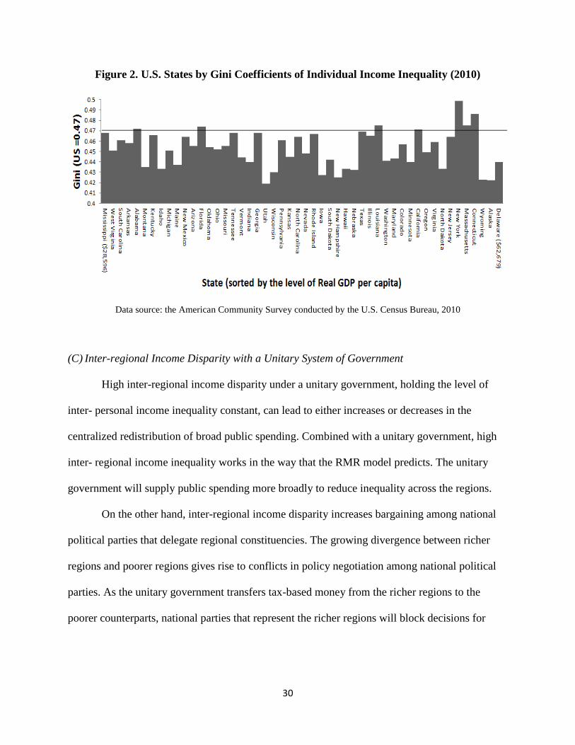
Compared to the inter-personal inequality which is explained by a relative poverty gap
between the median income and the average income, inter-regional inequality describes a
relative poverty gap in more complex ways. It captures not only relative poverty between
individual residents within a region but also relative poverty between regions. There will be
poorer individuals and richer individuals in each region. Because of relative homogeneity within
a region compared to across regions, the level of income inequality within a region is lower than
the level of income inequality in the entire country. This simplified assumption makes poorer
individuals in richer regions relatively wealthier than poorer individuals in poorer regions. For
example, Figure 2 compares the Gini score for the United States with Gini scores by the U.S.
state-level in 2010. On the horizontal axis, we see the level of inequality within a state. In most
cases, Gini scores by state-level are lower than the Gini score for the entire United States (0.47).
30
Figure 2. U.S. States by Gini Coefficients of Individual Income Inequality (2010)
Data source: the American Community Survey conducted by the U.S. Census Bureau, 2010
(C) Inter-regional Income Disparity with a Unitary System of Government
High inter-regional income disparity under a unitary government, holding the level of
inter- personal income inequality constant, can lead to either increases or decreases in the
centralized redistribution of broad public spending. Combined with a unitary government, high
inter- regional income inequality works in the way that the RMR model predicts. The unitary
government will supply public spending more broadly to reduce inequality across the regions.
On the other hand, inter-regional income disparity increases bargaining among national
political parties that delegate regional constituencies. The growing divergence between richer
regions and poorer regions gives rise to conflicts in policy negotiation among national political
parties. As the unitary government transfers tax-based money from the richer regions to the
poorer counterparts, national parties that represent the richer regions will block decisions for

31
more broad redistribution of public spending (Aysan, 2005a/b).11 In achieving policy
coordination more effectively, the unitary government mitigates this tension by reducing the size
of broad redistributive public spending (Giuranno, 2009a/b).
(D) Inter-regional Income Disparity with Federalism
Under federalism, national decisions on the broad redistribution of public spending will
be made by politicians that represent geographic jurisdictions. At a higher level of inter-regional
income disparity, policy preferences will vary. A federal system with high inter-regional
disparity, when holding inter-personal income disparity constant, will make regional conflicts
more severe. Thus, policy gridlock is expected.
Given that regions trump individual redistributive motives under federalism, a higher
level of inter-regional income disparity will increase conflicts between poorer regions and richer
regions. Under strong federalism, political decision-making power will be dispersed in both
poorer regions and richer regions with mutual veto power. A high level of inter-regional
inequality in federalism will increase policy divergence across disparate regions. Thus, there will
be competitive veto points. In a situation of competitive veto player constraints, richer regions
will veto more public spending for broader redistribution. The policy supply of the national
government under federalism seeks to meet this demand from richer regions by attempting to cut
broad public spending, but this will be difficult when poorer regions also veto spending cuts as
11 In a relative poverty concept, poorer individuals in richer regions will pay more tax than poorer individuals in
poorer regions based on progressive taxation uniformly imposed by the unitary government. This implies that richer
regions pay relatively more than poorer regions as costs of broad redistribution in public education spending
increase.

32
they want more redistribution. The expected result is a policy impasse. More competitive veto
points at divergent inter-regional disparities will erect barriers to a policy change (either increase
or decrease) for the broad redistribution of public spending. Whether the level of broad public
spending is high or low, it will be locked in where it is (Treisman, 2000).
To summarize, the redistributive policy effects of inter-regional income disparity are
distinctive from those of inter-personal income disparity under federalism although we may not
see this difference in a unitary system of government. I emphasize that the policy effects of
inequality with federalism differ by the two types of inequality. High inter-personal income
disparity and federalism have a synergic effect to create more redistributive demands from
poorer individuals through multiple subnational governments. There will be greater policy
provisions for broad public spending than when there is only a unitary government. High inter-
regional inequality interacts with federalism to erect competitive veto player constraints. It will
then be harder to bring a change in the amount spent on public policies in which benefits are
broadly consumed inter-regionally.
This theoretical overview made several assumptions. First, richer individuals do not want
to subsidize poorer individuals in the broad redistribution of public spending, as poorer
individuals benefit more from the broad provision of public spending (Stasavage, 2005). Second,
a national government is expected to redistribute resources inter-personally (from richer
individuals to poorer individuals) and inter-regionally (from richer regions to poorer regions)
through the broad provision of public goods including public education spending (Tanzi, 2000).
Given this set of assumptions, I expect that high inter-personal inequality across federal
regions would create pro-poor redistributive policy pressure because the regions are the smaller
replicas (microcosms) of the nation with the highly-skewed income distribution of individual

33
citizens. The local constituency demand will push their representatives to exploit a national
common pool of public education spending in distributing benefits specific to their localities.
Therefore, the overuse effect of common property can be an increasing linear function of the
number of regional delegates in the national legislation. These regional delegates engage in pork-
barrel politics making their benefits outweigh their equal share of the costs attached to
maintaining the national pool. The subsequent effect will lead to more public education
spending.
Hypothesis 2: Inter-personal income disparity in federalism, holding inter-regional
income disparity constant, further increases the level of broadly redistributive public
spending, more so than in a unitary system of government.
On the other hand, federalism for inter-regional inequality results in a third assumption:
redistributive motives among individuals are clustered upon their geographic locations.
Federalism fosters the dispersion of national policy decision making in political jurisdictions
with mutual veto power. Power dispersion shapes policies as a manifestation of inter-regional
inequality. Locally elected politicians will seek to enact national educational policy reflective of
a region’s specific demands. More competitive veto points with divergent regional interests will
create smaller bargaining space over the redistributive policies. Richer regions will veto more
spending, whereas poorer regions will veto spending cuts. High inter-regional inequality will
make veto player constraints worse. Changes in public education spending will be difficult. I
expect that the magnitude of policy change is smaller under federalism than in a unitary system
of government.

34
Hypothesis 3: Inter-regional income disparity in federalism, holding inter-personal
income disparity constant, leads to less change in public spending for broad redistribution
than in a unitary system of government.
This logic of redistributive conflicts expressed in a joint effect of inter-regional income
disparity and federalism on public spending for broad redistribution is limited in its policy scope.
Redistributive public programs are not monolithic but rather multidimensional. Indeed, they vary
from redistributive goods that are more directed to individuals (e.g., social security transfers and
healthcare) to redistributed goods that are more broadly consumed for the entire society (e.g.,
public safety and national security). In the following section, I further elaborate how the disparity
in regional economies and regional autonomy (defined as the authority of regional government
more broadly to capture the various policy dimensions of targeted spending) jointly shape
patterns of national policy outcomes over a range of choices on redistributive policy programs.
Policy Targeting: Preference Convergence among Disparate Regions with Policy Autonomy
Out of competing public budget categories, rich regions and poor regions are likely to
find it easier to coordinate their preferences for a social allocation in which benefits are directed
to specific individuals within every territorial region. Rich regions seek an increase in the
centralized redistribution of social spending, only as preferable to other types of redistributive
spending that go disproportionally to poor regions, especially when interregional inequality is
very high.12 For example, in the U.S., rich and unequal states such as California and New York
12 Similarly, rich regions seek the centralized redistribution of goods targeting specific individuals regardless of
geographic locations preferable to policy goods that are disproportionally geographical based.

35
are for increased social welfare spending nationwide although this policy choice creates a
spillover effect across other poor states. Regional transfers (benefits that are more broadly
redistributed for the entire society) redistribute taxpayer money away from a state like California
towards a relatively poor state such as Mississippi. Social transfers such as Medicaid (benefits
that are more directed to specific individuals) also benefit California. For poor regions, on the
other hand, interregional transfers are preferred to social transfers. As inter-regional income
disparity increases, individual beneficiaries of social transfers are larger in number and thus the
benefit of the policy program outweigh the costs of national policy coordination with their rich
regional counterparts. Thus, poor regions have an incentive to support more social transfers.
The authority exercised by regional governments over their territory and people intervene
to solidify their policy coordination on the central government’s budget allocation toward social
categories. This regional authority encompasses not only political representation and tax rate
control, but also it accounts for borrowing autonomy from the centrally imposed restrictions
(Hooghe et al., 2015).13 Regional authority is granted through constitutional rules of
policymaking. It facilitates a reactive power which blocks or delays a policy change away for the
status quo (Triesman, 2006). National representatives of regions endowed with this reactive
power can affect less-preferred expenditures by acting as veto gates for budget policies (e.g.,
upper house veto or amendment of lower house budgets and supermajority rules).
Rising inter-regional income disparity in a polity where regional authority is
institutionalized at a greater degree creates an increasingly cooperative policy incentive among
13 I assume federalism to be a subset of regional authority in a broader scope. I use two terms interchangeably. They
create institutional power that provides opportunities for regional representatives to influence national policy
making.

36
those unequal regions on greater budget allocation toward targeted spending. Given trade-offs
among competing budget categories, the policy pressures escalated by severe inter-regional
income disparity interacting with strong regional authority makes budget allocation towards
targeted spending more appealing to national representatives of regions and thus increases the
likelihood of a policy compromise among them.
Redistributive tensions between the rich and poor Länder in Germany provides an
illustrative case. Germany has high inter-regional income disparity linked to the German
reunification. For example, “in 1991, the GNP per capital in the new Eastern Länder was 30% of
that of the Western Länder” (Renzsch, 1998: 127). Through the German Unity Fund, allocation
of reunified Germany was heavily favored social spending involving for social assistance
(Sozialhife)14 as the form of redistribution which benefited the poor in the affluent Western
regions while also subsidizing the poor in the Eastern regions (Flockton, 1999). In fact, in the
period 1990-1994, Germany’s growth in social security transfer measured as a share of GDP
shows a much faster pace than the OECD’s with an average difference of 15 percent (Beramendi,
2012). Rich regions in Germany benefited somewhat from redistributive social spending but not
from redistributive public work projects. On the other hand, a political consequence brought
about by reunification was a stronger coalition in the upper chamber (Bundesrat) between the
Eastern Länder and poor Western Länder. During a policy negotiation over interregional
transfers primarily to the East (e.g., the Solidarity Pact starting in 1995), reunified Germany
facilitated a stronger institutional position for those contributing to Western Länder (Beramendi,
2012; Gunlicks, 2002). Given this constraint, targeted spending towards policies like social
14 Programs and services provided by local authorities directly to individuals who have exhausted their rights to
receive the unemployment compensation and need basic care in their daily lives (Beramendi, 2012).

37
Figure 3. Policy Effects of Rising Economic Disparities among Autonomous Regions
assistance is an opportunity for rich Western regions to shift allocation to their advantage while it
serves the policy interests of the poor Länder in the union. This interest convergence in policy
preference is predicted in hypothesis testing:
Hypothesis 4: Increased inter-regional inequality and regional authority prompt relative
allocation towards targeted spending in which benefits are directed to individuals.15
15 Inter-personal income disparity’s combined effect with regional authority does not matter to more targeted
spending because the majority poor from economically homogenous regions (by the assumption of inter-personal
income disparity are the beneficiaries from both targeted spending and broad non-targeted spending.

38
Figure 3 illustrates the expected joint effects of severity in regional inequality and
strength in regional autonomy on the relative amount of targeted spending in which benefits
more are directed to individuals across all territorial units. With a rise in the severity of regional
inequality, the strength of regional autonomy should be positively correlated with the size of
relative budget allocation towards targeted spending.16
To summarize, this chapter theorizes inter-regional inequality as conceptually distinct
from inter-personal income disparity. I describe individual redistributive motives by economic
geography and then apply this theory to the political logic of redistributive conflicts. A
discussion on the intervening role of regional autonomy also helps to identify a condition under
which disparate regions’ redistributive conflicts among disparate regions lead to policy gridlock
or a policy compromise. The next three empirical chapters present supporting evidence and
policy implications.
16 Although not shown here, I assume a symmetry of interaction that as the strength of regional authority grow,
severity in regional inequality is also increasingly correlated with relative targeted spending.

39
CHAPTER 3
Spatial Patterns of Individual Support for Public Education Financing:
Evidence from South Korea
Regions differ by their level of income as well as their internal distribution of income.
These differences affect the redistributive interests of their residents. In the previous theory
chapter, I explained how an economic disparity in regional income could shape a policy alliance
between individuals with preferences for redistributive spending. The crux of my argument here
is that both poor and rich residents in the poor areas prefer higher levels of public spending.
These geographically clustered people demand higher central government expenditures, which
are financed by centralized taxes and redistributed across economically disparate regions of a
country. The poor in the poor regions want it because they are likely to be net beneficiaries of
this centralized redistribution, and the rich in the poor regions want it because it offsets the tax
burden to support their poor neighbors which they would otherwise fund by themselves at the
local level. In comparison, residents in affluent regions are likely to prefer having their tax
revenues spent within their regions. More central redistribution requires higher central taxes,
which becomes burdensome for the rich taxpayers from the affluent regions. The marginal gains
of the poor in affluent regions decrease with broader centralized redistribution because they
share the benefits with the poor in the other regions.
To test these regional characteristics influencing the redistributive interests of
individuals, I performed a series of regression analyses. The associated sample data was drawn
from a recent Korean General Social Survey (KGSS) regarding citizen preferences for increases
in public education spending, a policy that is highly centralized in administrative proceedings.

40
To explain the variance of individual preferences across regions, I use the survey respondent’s
residential information. The analysis presented below offers strong evidence that both rich and
poor residents in poor regions support higher public education spending, whereas those in
affluent regions tend to oppose expansionary spending. This empirical result suggests that
regional wealth disparity trumps the redistributive motives of individuals.
The remainder of this survey data analysis is organized as follows. First, I begin with a
case that describes a top-down administrative structure of resource allocation deeply rooted in
Korean public education financing. Second, I offer a brief literature review on the relationship
between income inequality and public spending. This following section details my hypotheses
and their theoretical foundations. Third, in the data section, I describe details of the KGSS data’s
variables and measures. Then, the following section presents the results from my regression
analyses. Lastly, I discuss policy implications of the findings.
Case Selection: The Structure of Public Education Financing in South Korea
The finance of Korean public education is highly centralized.17 Most funding for local
school management costs comes from the central government’s grants and subsidies, equivalent
to roughly 20 percent of the country’s total internal revenue. Additional funding is also available
on the revenue of the education tax, which is levied as surtax on many other types of national
17 In this chapter, I set the analytic scope of public education restricted to public and non-tertiary sectors only, given
that private sources play a much bigger role in financing tertiary education in Korea. For instance, in 2001, 73
percent of tertiary education funds came from private sources. This number is considerably larger than the OECD
average of 31 percent (see OECD Education at a Glance 2014).

41
Figure 4. Centralized Structure of Education Financing in Korea (2006)
taxes including, for example, the gasoline tax and the transportation tax.18 This fund is managed
by the Ministry of Education (MOE). Additionally, there is a small portion of revenue coming
from fees and tuition paid by the students and their parents.
As illustrated in Figure 4, the educational administration of Korea has the three-tier
structure comprised of the central management (i.e., MOE), the macro-local administrative
divisions (i.e.,16 metropolitan and provincial offices of education), and the local subdivisions
(i.e., 180 regional offices of education). The autonomy of local education services is
18 Some education revenue is collected at the local level, although it is much smaller in scale. However, this
localized function is operationalized in a centralized manner. For example, the revenue of Local Education Tax
collected by local governments goes to the Local Education Special Account, a revenue source of Offices of
Education at 16 prefectures over which the central Ministry of Education takes full control.
180 Regional Offices of Education: Funding Mostly Tranferred to Teachers' Salaries in Local Schools.
16 Metropolitan and Provincial Offices of Education (as Administrative Arms of
MOE)
The Ministry of Education (MOE) Budget at the Central Goverment.
20% of internal tax revenue allocated for local governments' education budgets.
Education Tax Revenue (as Surtax)
Budget Planning and Administrative Decisions
80% of thier revenue transferred from the MOE
Other revenue (small degree) transfered from local governing bodies, internal assets, locally issued bonds, school admission fees and tuition.

42
institutionally promoted by electing the head of the local office of education directly in the local
election. However, the authority and responsibility are still financially centralized between these
offices of education. For instance, regional offices of education receive roughly 80 percent of
their revenue (primarily going to the payment of teachers’ salaries) from the grants and subsidies
of the MOE. Also, 16 prefectural educational offices, under which regional offices are
administered, act as administrative arms of the MOE regarding budget planning and decisions.
The continuity of centralized public education finance is mainly attributed to the “blurred
nature” of expenditure responsibilities between the central and local governments (Kim, 2004).
Although Korea has a full-fledged local autonomy system (started in 1995) for balanced regional
development, the fiscal decentralization has been unclear in policy implementation. There are
two reasons for this lingering policy problem, particularly in the domain of public education
finance. First, the Korean government has long pursued public education as an egalitarian tool
for the public regardless of geographic location or socio-economic status.19 The second reason
concerns the coordination issue of strategic interest. For the central government, practicing a
system of centralized redistribution creates opportunities to exert its fiscal power over local
governments. By coalescing to this policy intervention from the center, local governments
19 See an introductory note by Byun (2010) for two long-run policy examples: 1) Education Tax Act (in 1958) for
free compulsory primary education; 2) high school equalization policy (HSEP in 1974) with the introduction of
random school assignment. In the region adopting the HSEP, the middle school graduates are assigned to a high
school within their residential areas based on a random computerized lottery. In case of the regions not adopting the
HSEP, public high schools generally select their students through region-wide high school entrance exams or middle
school transcripts.

43
reserve an institutional channel to ask for more intergovernmental transfers whenever needs for
local expenditure are greater than supplies of locally raised funds.20
Theoretical Frame: Individual Income Positions and Preferences for Public Education
Subsidies
Starting from the seminal contribution of Meltzer and Richard (1981), scholarship in
political economy has shown that individual preferences for redistribution may be inferred from
an individual’s position in the distribution of income. The relevant works by Boix (1997, 1998)
and Ansell (2008a/b, 2010) apply this frame to the study of education. The poor like to support
funding for education because the tax-funded money goes to those who are at the lower end of
the income distribution. On the contrary, the more well-off individuals, who have a greater
ability to opt out for private education, tend to oppose increases in public education subsidies
that are funded by tax hikes.21
20 These cases are quite common, especially among the poor regions having fiscal difficulties to meet increasing
demands, given that local taxation is virtually fixed in Korea. See a similar view in McLure (2001) and Bird &
Tarasov (2004).
21 The redistributive policy preference from income position over publicly financed education is not always clear-
cut, however. The lower income class might prefer more spending on other social policies instead of education
spending, depending on the degree of their demands and expectations for immediate redistributive consequences. As
for the wealthy, they might support the expansion of public subsidies to education when they expect more benefits
from it (e.g., increased labor productivity via the promotion of public access to education) than from other social
policies, or when they need to pay for private education at very high costs (Fernandez & Rogerson, 1995; Ansell,
2008a/b). Therefore, as argued by Levy (2005), if the aggregated effects of income position are tested against

44
These micro-foundations of individual policy preferences, however, have largely ignored
interactions with macro-institutional contexts that affect the relative pay-offs of public
investment in different income classes. This macro-micro joint relation has received little
attention among previous studies that have attempted to identify determinants of preferences for
education spending. Exceptions are partially provided by more recent scholarship (e.g., Ansell,
2010; Busemeyer, 2009, 2012; Busemeyer & Iversen, 2014; Kitchelt & Rehm, 2006). These
pertinent works hinted that the impact of the individual income position on education preferences
strongly depends on the interplay between the individual’s position on the income scale and the
types of institutional arrangements (e.g., representation systems, partisan participation in
government, and existing levels of socio-economic /educational stratification).
Although this multilevel research has significantly contributed to a better understanding
of individual- and institutional-level determinants of policy preferences, there has been a lack of
discussion about the impact of spatial (or more precisely, geographic) contexts on the micro-
level dynamics of preference formation. This is an important omission, especially for the
discussion of individual policy attitudes towards the education subsidies redistributed from the
central government. Inequality in the asset distributions across regions sets the price for the
income share contributing to education investment at different marginal costs (Beramendi &
Rehm, 2016), and this relative price is likely to constrain the central government’s provision
(Wibbels, 2005). As argued by Kim (2006), the wealthy regions view redistribution by the
central government as expensive because they pay for the services (or resources) that are
education preference in fiscal terms, an individual’s income position as such may not necessarily serve as a
significant determinant.

45
transferred to their poor counterparts. On the other hand, poor local governments may interpret
this transfer as a process to guarantee them more fiscal resource inflows.
As an extension to this locality-based research, my focus lies on the policy effects of
macro contexts interacting with the micro-level dynamics of preference formation. To be
concrete, my contextual approach examines the role of regional economic disparity (macro-
component) in shaping the way that an individual’s income position (micro-component)
determines preferences on education spending. I place emphasis on the role of disparity in
regional wealth as a key macro-level determinant of individual preference for public education
investment. I argue for more (less) support among residents in poor (rich) regions. The
centralized redistribution of tax-funded money makes these people net beneficiaries
(contributors) at the price they pay for sharing the public provision of education spending.
Survey Data for Empirical Validation
To examine how individual income positions in the context of regional wealth may affect
individual policy preferences for public education spending, I use the Korean General Social
Survey (KGSS) data collected in 2006. The dataset includes the most recent information about
individual attitudes towards increases in education subsidies by the central government.
Respondents’ geographic locations are identified at the municipal level.22 To be specific, the
KGSS includes the following question about preference for more public education spending:
22 Samples were collected for the population over the age 18 across 96 subnational regions at the municipal level. To
do so, the survey used a multi-stage area cluster sampling method for a total of 1605 interviews.

46
Please show whether you would like to see more or less government spending on education.
Remember that if you say “much more,” it might require a tax increase to pay for it.
1. Should spend much less
2. Should spend less
3. Should spend the same as now
4. Should spend more
5. Should spend much more
Figure 5 (below) summarizes the overall distribution of individual preferences for education
subsidies provided by the central government.23 The average preference level is around 3.8 on a
five-ordinal scale moving from “spend much less” to “spending much more.” The response share
of each category amounts to 26.2 percent for “spend much more,” 43.0 percent for “spend
more,” 21.1 percent for “spend the same as now,” 6.4 percent for “spend less,” 0.6 percent for
“spend much less,” and 2.7 percent for “don’t know.”24 From an overall perspective of the KGSS
samples, a majority of the survey respondents show their support for spending increases (rather
than decreases) in general, regardless of policy categories including environment, health, law
23 The survey respondents do not necessarily know at which government level funding for public education is
collected and redistributed. The survey did not specify nor provide information before the query was exposed to the
respondents.
24 “Don’t know” answers are excluded from the analysis. Including them in the same category as “spend the same as
now” did not alter key findings in any meaningful ways.

47
Figure 5. Variations in Public Support for Education Financing
Source: KGSS 2006 (96 Municipal Regions)
Government should spend money: education
enforcement, education, and retirement pension.25 This general pattern for pro-spending attitudes
applies to the survey questions including the area of public education, where support for
increases in education subsidies reached almost 69 percent of the total responses. Education is
25 See for a similar case in Jacoby (1994)’s study of the American public opinions. By and large, the respondents
showed a desire to have a small government but in terms of spending questions pertinent to a specific policy
category, they show strong preference for spending increase rather than decrease.

48
the largest portion of public support for any policy category examined in the survey
questionnaires. One way to interpret this positive number is that people perceive increases in the
public provision of education subsidies as a channel for equal opportunities (note that we saw
this aspect earlier in the Korean government’s key policy agenda). But at the same time, people
may also see such increases as an important economic engine for human capital development
(Park, 2008). Nonetheless, it is plausible that respondents are aware of the increased tax burden
associated with increased spending (as it was mentioned within the survey question). The
“spending much more” category was only about half the percent as those for large spending (26
percent vs. 43 percent), perhaps because respondents are reminded of the tax burden at that
category.
The second reason for my use of the KGSS data is that they provide valuable
demographic information regarding each survey respondent’s geographic location by
administrative districts (the survey assigned each respondent with a block number indicative of a
municipal region). The geographic data are broken down into 96 regional locations at the
municipal level. 26 This information allows me to examine the spatial distribution of individual
preferences for education spending. My expectation is that the people in the rich metropolitan
areas will be relatively unsupportive of the broad redistribution of public education subsidies,
compared to the people in the less developed regions.
Figure 6 presents scatter evidence among subnational regions in their proportional
differences in total respondents who answered, “should spend much more.” For instance,
Pyeongtaek-si (a suburb region) had 63 percent of the respondents for expansionary education
26 I used the municipal level identification for the survey respondents in order to closely match them with their
electoral districts at a local level.

49
Figure 6. Geographic Distribution of Public Support for Education Financing
Source: KGSS 2006 (96 Municipal Regions)
Notes: Administratively, local governments are divided into a total of 16 prefectures and 234 municipalities. Prefectures, upper-
level local governments, are composed of a metropolis (Seoul), six wide-area cities (Busan, Daegu, Incheon, Gwangju, Daejeon,
and Ulsan), and nine provinces (Gangwon, Kyonggi, Chungbuk, Chungnam, Jeonbuk, Jeonnam, Gyeongbuk, Gyeongnam, and
Jeju). Municipalities consist of cities, towns (Gun), and special districts (Gu). Cities have a population of 50,000 or more, and
towns (Gun) have a population of under 50,000. Special districts are autonomous municipalities under seven big cities (Seoul and
Six wide-area cities).

50
spending, while Secho-gu in Seoul (a capital region) showed that the supporters were only about
33 percent of all responses. Please see Appendix 2 for additional contrasts with other regions in
urban Seoul, which ranges from 20 percent (Jungnang-gu) to 50 percent (Gangbuk-gu).
However, as illustrated in Figure 6, this stark contrast is not always the case, as can be seen in
the comparison between rural districts and six additional metropolitan cites other than Seoul.27
For example, the KGSS survey data collected from Yeongdo-gu—a densely populated district of
Busan, which is the largest port city of South Korea—show that roughly 57 percent of the survey
respondents expressed a strong preference for expansionary spending on public education. This
number is only marginally different from the approximation describing Pyeongtaek.28
Dependent Variable
My empirical research is interested in the behavioral patterns of individuals reacting to
tax-funded spending for public education. Given that, I used a binary coding for representing
“spending much more” with a tax burden reminder, instead of keeping the original five-scale
index (spend much more, more, the same as now, less, or much less).29 The methodological base
for such binary coding follows a contingent valuation method (CVM) that can measure demands
for public services by asking the survey respondents about their willingness to pay for the
27 This is also called six “wide-area” cites, listed as Busan, Daegu, Daejeon, Gwangju, Incheon, and Ulsan. Please
see Figure 6 for their geographic reference in Korea.
28 Defined by the intra-regional distribution of public resources, the net benefit to individuals remains
disproportionate with the size of the local population. Intergovernmental transfers may offset some of the negative
impacts of population density. Fortunately, the sample weight was applied to the KGSS data as indicated in the
survey methodology section, although the weight variables are publicly unavailable.
29 A robustness check for the ordinal scales is reported in Appendix 6.

51
services. This CVM-type survey is common in the works that address a type of value placed by
citizens on education (Mitchell & Carson, 1989; Duncome et al., 2003). Nearly 25 percent of the
KGSS’s respondents support expansionary spending on public education, even at a risk of a
higher tax burden. See Appendix 2 for the binary data distribution by municipalities, which
ranges from 0 percent (Gimpo-si, near Seoul) to 63 percent (Pyeongtaek-si) in support of a major
tax-funded increase in education spending.
Independent Variables
The independent variables of interest are four groups of individuals, defined by their
place in the income distribution (both in the national and region distribution), and by the overall
income of their regions.30 First, I grouped residents according to their position in the nationally
aggregated income distribution as poor residents in poor regions (Pp), rich residents in poor
regions (Rp), poor residents in rich regions (Pr), and rich residents in rich regions (Rr). Then I
modified these group identifiers (PP, RP, Pr, Rr) into the categories of individuals’ relative income
positions within their region (P̅P, P̅r, R̅P, R̅r). I provide greater detail about these identifiers in the
following pages (See Table 3 below for a summary).
Distribution of National Wealth across Regions
The relevant macroeconomic context is inequality in the distribution of national wealth
across geographic regions (henceforth called economic geography). To measure economic
30 The interaction between the individual’s income position and the distribution of the regional wealth can be
constructed as a continuous variable, but this does not allow for me to identify four different groups from the
estimation model all together.

52
geography, I use the regional index of financial independence from the central government. I
measure fiscal independence rather than a direct measure of income because the regions’ fiscal
resources (which might not be closely related to wealth) are closer in theory to the analysis at
hand. Regional residents’ view of policy funded at the central level should be compared to the
funding available in their region. The municipal level data were obtained from the Korean
Statistical Information Service (KOSIS) portal. This index is a ratio of the municipal
government’s own-source revenue to its total revenue. The higher ratio the local government has,
the more independently it functions from the central government subsidies.31 A high tax ratio
also suggests that a region is rich. Simply for inferential convenience, this ratio index measure is
converted to a percentage. It covers the total of 96 municipal regions from which the KGSS data
were collected. It shows a range from 10.1 (Yechen-gun, a rural region) to 90.4 (Secho-gu, a
capital region). In Seoul only, Gangnam-gu (one of the richest regions located on the south side
of the Han River) is almost 2.8 times more financially independence than Jungnan-gu (one of the
relatively less affluent regions located on the north side of the Han River). See Appendix 2 for
additional details on regional variation.32
31 Rich regions often receive large fiscal transfers from the central government as part of the initiative to boost local
economic development. Based on the financial independence formula (i.e., given as own-source revenue divided by
total revenue), such transfers are inversely proportional to the rich region’s level of fiscal independence. However,
in many cases, rich regions are also densely populated. In other words, more own-source revenues are anticipated
form their tax bases. The correlation between the size of the regional population and the index of financial
independence is 0.75 (p <0.05).
32 Apparently, it not necessarily the case that the densely populated municipal regions show a high ratio in the
financial independence index. This is because these regional areas are often recipients of the central government
subsidies due to increasing public demands from their large populations.

53
On disparities in regional wealth, each region was assigned to a decile rank by the level
of financial independence. Note that I did not use a direct measure of regional finance here
because the policy effects triggered by the poor and the rich jurisdictions do not necessarily rely
on a linear assumption due to the (typically right) skewed distribution of regional wealth. In
comparison, a decile rank makes it easier to create different profiles for the disparity in regional
wealth. In practice, municipal regions ranked at the top 20 percent in the distribution of the
financial independence data are considered economically well-off (notated as a subscript of r).
Whereas, those ranked at the bottom 20 percent are considered economically destitute (notated as
a subscript of p). Dummy coding was applied to the variables capturing these two regional
groups, with notions of r and p.
Distribution of Individual Incomes
To show individuals’ positions in the nationally aggregated income distribution, I used
the KGSS data on the monthly income (before tax and other deductions) of the respondent’s
household—values weighted for the size of their household. The household income measure is
used to maximize observations and is a better indicator of individuals’ overall economic
conditions than is individual income (see also Busemeyer et al., 2009; Busemeyer & Iversen,
2014). To distinguish rich (henceforth, denoted by a capital letter R) from poor (denoted by a
capital letter P), every survey respondent was assigned to a decile rank by his or her level of
household income. This rank information is coded in two dummy variables (i.e., the rich ranked
at the top 20 percent, and the poor ranked at the bottom 20 percent). 33
33 As a robustness check, I also adopted a different threshold value (e.g., the top 40 percent and the bottom 40
percent in the distribution of household income). See Appendix 4 for consistency.

54
Table 3. Summary of Household Income Distribution by Regions
Distribution of Household Income among Individuals
(Nationwide)
(Region-specific)
Poor (P) Bottom 20%
Rich (R) Top 20%
Poor (P̅) Bottom 20%
Rich (R̅) Top 20%
Distribution of
National Wealth
across Subnational
Regions
(Nationwide)
Poor (p) Bottom 20%
P p R p P̅ P R̅ P
Rich (r) Top 20%
P r R r P̅ r R̅ r
In short, the group identifier box that sits on the left side of Table 3 illustrates four
different income groups. These are solely based on the individual’s position in the nationally
aggregated income distribution. Pp, for instance, may be equivalent to those destitute poor living
in a remote rural area. On the other hand, Rr represents those who have high earning jobs and
live in an affluent region like Gangnam-gu in Seoul (similar to Beverly Hills in Los Angeles,
California).
The group identifier box that sits on the right side of Table 3 differs in nature by relative
income specific to regions. I assigned the decile rank information of household income
distribution among individuals according to their relative positions in the region-specific income
distribution. To avoid confusion with the nationwide income rank, I applied a new notation for
household income rank specified by regional scope: P̅P < R̅P (written as poor and rich residents
within an impoverished region, respectively) versus P̅r < R̅r (written as poor and rich residents
within an affluent region, respectively). This rank order is in part similar to what we saw earlier
from the household income rank, based on the nationally aggregated distribution (Pp = Pr < Rp =

55
Rr).34 However, when considering relative income positions specific to regions, the former
should differ from the latter in various ways: for example,
either P̅P < P̅r < R̅P < R̅r or
P̅P < R̅P < P̅r < R̅r , or
P̅P < (R̅P = P̅r) < R̅r.35
In simple terms, this implies that the poor in rich regions, P̅r, may earn more or less than (or
equal to) the rich in poor regions, R̅p. In contrast, according to an intra-regional perspective, it is
certain that the earnings of P̅r are less than those of R̅r.
The earning of R̅r (region-specific) should also be bigger than that of Rr (nationwide). As
a real data example from the KGSS in 2006, a group of individuals holding income attributes of
R̅r corresponds to Gangnam-gu’s top 20 household income holders. The data show that these
34 According to the nationally aggregated income distribution, individuals holding the same level of household
income are simply geographically dispersed. In other words, some people living in a wealthy region (Pr) are as poor
as those staying in a poor region (Pp). In fact, an urban area typically shows higher interpersonal inequality than a
rural area. For example, this assumes that Pr may earn an equivalent income to Pp.
35 There are other possibilities for the income rank order as described below.
1) P̅P < P̅r < R̅r < R̅P (e.g., the millionaires living in rural areas)
2) P̅r < P̅P < R̅P < R̅r (e.g., the destitute poor living in urban ghetto areas)
3) P̅r < P̅P < R̅r < R̅P (e.g., conditions 1 and 2 combined)
However, for the sake of model simplicity, in this research I treat these additional cases as outliers. This means that
my analysis begins with an assumption: on average, P̅P is a group of the poorest individuals where as R̅r is a group
of the richest individuals in their income status nationwide. Moreover, this assumption matters for my analysis
focusing on the costs and trade-offs associated with P̅r and R̅P, depending on the regional outlook of income
distribution.

56
individuals mostly had high earning jobs varying from administrative associate professionals to
trade brokers. R̅r’s average monthly income amounted to $10,837 (converted from Korean won
in 2006). This amount is roughly 4,000 dollars more than the average household earning of Rr
($6,983). As such, the real data difference between R̅r and Rr reveal that relative income strata
vary, depending on the geographic locations of unequal income holders.
To ensure that the earning of R̅r is greater than that of R̅p, I checked the KGSS data.
Seocho-gu, which makes up the greater Gangnam area along with Gangnam-gu, is on the
southern side of the Han River. The KGSS data identifies R̅r (Secho-gu’s top 20 household
income earners) as having an average monthly holding of $19,530 in 2006. This dollar amount is
almost five times bigger than the average monthly earning of R̅p in Jungnang-gu (a less affluent
region on the northern side of the Han River in Seoul). The average monthly household income
of R̅p in Jungnang-gu was $4,515 in 2006. This relative income level tendency toward R̅r > R̅p
implies that the rich in affluent regions earn more than the rich in less affluent regions.
According to the KGSS’s additional household income reports, the bottom 20 percent of
household income earners (P̅r) in the greater Gangnam area was found to have average monthly
income holdings of $3,440 (Seocho-gu) and $989 (Gangnam-gu). These amounts are much
larger than the average monthly income holding of P̅P from Haenam-gun, which ranks as the in
the distribution of financial independence (See Appendix 2). In 2006, Haenam-gun’s bottom 20
percent household income earners maintained their average holding of $215 per month. This
relative income portion suggests that, in general, the poor in poor regions have fewer earning
opportunities than do the poor in rich regions.

57
Table 4. Summary of Expectations on Support for Increased Education Spending
Household Income
(Nationwide)
Household Income
(Region-specific)
Poor Rich Poor Rich
Regional
Wealth
Poor [Pp] + [Rp] + Poor [P̅P] + [R̅P] +
Rich [Pr] - [Rr] - Rich [P̅r] - [R̅r] -
The cross check (nationwide vs. region-specific) available from Table 4 helps to yield
predictions about policy preferences of two focus groups in particular: Pr and Rp (also with P̅r
and R̅p). First, applied to the nationally aggregated income distribution scheme, Pr could be
identical to Pp regarding their cost sharing at the same rate of taxation that goes to the national
government’s vault.36 However, Pr could benefit greatly from the large tax contribution by Rr
(given an income level where Rr > Rp), which would help to offset a fixed cost (determined by a
progressive tax rate) incurred to them as long as all available funds for public education were
collected and redistributed intra-regionally rather than nationally. This yields the expectation that
Pr dislikes or at least remain unsupportive of increasing funding for public education that is
shared across regions.
36 Note that this scenario excludes a case in which Rr is also simultaneously identical to Rp at the rate of tax pay. In
such a case, it would assume the same income distribution in every region; hence there would be no distinction
between the rich regions and the poor regions, but rather it would assume one single polity (Meltzer & Richard,
1981).

58
The second prediction also rests on the nationwide income distribution base. The cost of
raising funding for public education could be fixed at the same rate of progressive taxation to
both Rp and Rr. Nonetheless, as for Rp even at the fixed cost, having high local demands from
their poor population would make every single penny of spending worthless towards the quality
improvement of public education unless there are additional contributions from Rr. In other
words, national redistribution to the poor region offsets local education spending that would be
borne by the Rp in a decentralized system. Thus, it is likely that Rp supports expansionary
spending when tax-funded money goes to the central government and gets redistributed across
regions broadly.
This method of scope allows for identifying differences in relative marginal return to
income earners, all depending on the economic geography of their residential locations.37 Several
additional predictions can be drawn from variations in income distribution by region. First,
defined by the region-specific income distribution, P̅r may earn more than P̅p, although it is
obvious that P̅r earns less than R̅r. Second, this assumes that P̅r pays more education tax than does
P̅p, according to the system of progressive national taxation in Korea. From this relative
difference in tax-funded cost among groups, one deduces a third prediction that is, to raise
funding for cross-regional public education, P̅r would have to contribute some of its income
distributions to P̅p, which would reduce P̅r’s net benefits after taking into account the tax
37 In Korea, the education tax collected by the central government is uniformly applied to all income earners at a
progressive tax rate. The costs incurred to these individual taxpayers, therefore, differ only by their income level,
and are independent of their geographic locations. However, location also matters when policy interest comes down
to net benefits, calculated on the basis of location (which assumes that income distribution differs by regions) and
the tax costs to be applied to individuals.

59
contribution by their wealthier counterparts. It is suggested therefore that P̅r might not have a
strong incentive to support increased education spending. The fourth prediction, also applying a
region-specific income distribution scheme, is concerned with the policy incentives of R̅p , visa
vie R̅r. Assuming that the income level of R̅p is lower than that of R̅r, R̅p’s share of income
supplemented by funding from R̅r to finance cross-regional public education would offset costs
to providing education for their local P̅p. Individuals in R̅p pay a fixed amount of tax, but their net
benefits differ depending on whether they have a system of redistribution that includes R̅r or not.
Based on this, we expect that R̅p would support more funding for education when the benefits are
redistributed cross-regionally.
To incorporate this set of expectations into the model estimating all types of cross-level
relations between individual income positions and economic geography, I use dummy variables
to code for nationwide factors of Pp, Rp, Pr, and Rr (also similarly for region-specific factors of
P̅p, R̅p, P̅r, and R̅r). For instance, Pp is assigned a value of 1 if the respondent’s income attributes
match the description of poor residents (P = 1) and poor regions (p = 1). Otherwise, a value of
zero is assigned. Following in this way, I constructed 4 dummy variables to be used together in
the regression analysis, with the middle-income earners omitted as the reference category.38
38 I purposefully chose the middle-income earners as the reference category because their preferences for
redistributive policies are rather tricky when thinking in terms of the structure of disparate income positions. As
demonstrated in the social affinity theory adopted by Lupu and Pontusson (2011), the middle class’ relative income
distance to the poor, compared to their distance to the affluent, is likely to determine public support for redistributive
policies. In addition, from a modeling perspective, the use of middle income earners as the base allows the model
incorporating all of the spatial relations discussed here to be used. In this regard, I implicitly consider Pp (P̅p) >
middle income earners > Rr (R̅r) in their preference orders regarding increases in funding for public education.

60
Controls
To isolate the effects of Pp, Rp, Pr, and Rr (and the effects of P̅p, R̅p, P̅r, and R̅r) on public
preferences for education spending increases, I employ several socio-demographic control
variables (all individual-level data) drawn from standard public sector demand models.
I take into account several alternative explanations for variations in individual
preferences for public education spending. Gender is one factor thought to affect an individual’s
support for social spending.39 It is often argued that women are more likely to favor social
spending since such public expenditures may create more opportunities for women to engage in
the active labor force (Park, 2008). Since women tend to earn less than men, we may expect
them to favor more public education spending (Busemeyer & Iversen, 2014). Female
respondents are assigned a value of 1, and zero otherwise.
College graduates are likely to support higher spending for education budgets (see
Duncombe et al., 2003). Moreover, statistics show a significant earning gap between high school
and college graduates, and this gap highlights the importance of public schools’ preparation not
only for employment but for higher education as well (Plutzer & Berkman, 2005). To capture
these individual traits, I assigned a value of 1 to all survey respondents who held a 4 year college
degree or above.
The provision of publicly funded education is an attractive policy option for families with
school age children. Married with kids is a dummy variable used as a correlative of support for
39 The names of all control variables here are italicized for clarity. These variable names were not necessarily given
in exact phrase as part of the query to the survey respondents.

61
education spending.40 As a related control, seniors are more likely to oppose increases in public
education spending because benefits from these services do not go to them directly. For further
explanation, see the intergenerational conflict argument put forth by Preston (1996) and
Duncombe et al. (2003). I created a dummy variable using the respondent’s age information. A
value of 1 is assigned to all respondents over the age of 65 years.
Occupation in education fields is likely to produce positive impacts on preferences for
spending on public education. Research shows a positive correlation between support for school
budgets and being an employee of school districts (Duncombe et al., 2003). To distinguish
respondents who work in the education field, such as teaching professionals and school
inspectors, I use the KGSS’ variable on 4 digit ISCO-88 numbers offered by the International
Standard Classification of Occupation. This code identifies the respondent’s profession. All
professions associated with education fields within the ISCO-88 are assigned a value of 1, and
zero otherwise.
I also include a measure of the respondent’s ideological self-placement on the liberal-
conservative continuum to capture an individual’s political orientation towards the public share
in education funding. According to general explanations from political psychology, a more left-
ward 41 orientation is associated with a more liberal conception of human rights—i.e., a
40 For the sake of simplicity, dummy coding is used for attributes in the joint occurrence of the respondent’s marital
status (0/1) and their staying with children (0/1). To be more precise, I extracted the pertinent information regarding
school age children from the KGSS’s compound factors in demographic variables of family members (e.g., family
members’ ages and relationship to the respondent). I then re-ran the model with this alternative dummy. The result
did not change appreciably with this alternation.
41 Here, I loosely use the conservative-liberal self-placement as interchangeable with the right-left self-placement,
although the meaning of these dimensions may vary across nations (Dalton, 2006; Inglehart, 1990; Huber &
62
preference for respecting the rights of other individuals (Haidt & Graham, 2007). The ideological
self-placement data from the KGSS are scaled into the range from very conservative (1) to very
liberal (5).
Studies show more religious people, irrespective of their denominations, are less likely to
demand social spending because religious involvement can serve as an alternative to social
insurance for individuals (see, for example, Scheve & Stasavage, 2006; Benabou & Tirole,
2006). Individuals often draw communal material support in times of difficulty from their
religious participation. See for the relevant evidence in the case of the U.S. (Hungerman, 2005;
Chen & Lind, 2014; Dehejia et al., 2007). The respondent’s religiosity is measured as the
frequency in attending religious services.
It is also important to add factors regarding the respondent’s subjective evaluation of the
political economy, as it plays a role in shaping preferences for education. To incorporate this, I
draw on a series of attitudinal survey work conducted by Duncombe et al. (2003) and Park
(2007). When taxed at high rates, individuals are less attracted to increases in tax-funded
education spending. Tax burden for high-income will diminish individual preferences for
expansionary public expenditure. Moreover, support for preferential spending on education is
anticipated to rise when the public has a more positive prospect for future economies and when
they view quality public education as an engine for development. Thus, a prospective of better
economic conditions is likely to have a positive sign on preferences for expansionary education
spending. Also, in the sense that the public provision of quality education is often viewed as
Inglehart, 1995). Quite contrary to this, however, Kim and Kang (2013) found from their cross-cultural validity
study of self-rated political orientation that both Korean and American participations have common characteristics
in self-rated political ideology.

63
equal opportunity enhancing, those respondents having a stronger expectation for government
responsiveness are apt to assign a greater degree of preference to increases in public education
funds.
Model Specification and Estimation Strategy
Based on preferential policy data that has binary outcomes, I look into a series of probit
regression estimates of support for tax-funded education spending. I put all dummy variables
together into one estimation model to examine the contextual effects of income positions across
ninety-six Korean municipal regions.42 One could argue that a multilevel model is a better way to
control for factors specific to the regions. Typically, in performing the analysis, this alternative
method suggests that we take into account the estimation uncertainty regarding individual-level
outcomes due to variations between groups—in my case, such variations would be regional
differences in financial independence. However, in this research, I do not necessarily use a
region’s financial independence as a group-level predictor for explaining the averaged preference
among all individuals that may vary across regions. This averaged preference is not my research
interest. I am more interested in examining how a region’s financial condition affects region-
specific preferences of individuals with different income holding statuses. Thus, a probit model
design is more appealing:
42 I use probit estimators instead of logit because I attempt to model high preferences for education spending as a
function of covariates. The survey recorded for preferences themselves are designed to be normally distributed as a
sampling of the population. Yet, I dichotomize it during my empirical application (i.e., high preference in spite of a
potential tax burden or not).

64
Prob [High Preference i = 1] = Φ [β1 + β2 Poor Residents in Poor Regions
+ β3 Rich Residents in Poor Regions
+ β4 Poor Residents in Rich Regions
+ β5 Rich Residents in Rich Regions
+ ∑ βj𝑗 𝑋
+ ∑ βk 𝑅𝑒𝑔𝑖𝑜𝑛𝑘 + εi ]
where the dependent variable, High Preference, takes a value of 1 if an individual respondent (i)
from the KGSS in 2006 was willing to support increases in tax-funded public education spending
even with a potential for a tax increase. Otherwise, a value of zero is assigned to all other valid
individual responses collected across municipal regions in Korea. Φ denotes the standard
cumulative normal distribution.
βs represent a series of probit estimators to be estimated. β1 is the constant term. β2
through β5 are parameters that capture the policy effects of income positions contextually related
with types of economic geography (e.g., Pp, Rp, Pr, Rr or P̅p, R̅p, P̅r, R̅r). I expect the coefficient
estimates of β2 and β3 to show a positive sign on the predicted probability of high preference. By
comparison, the signs of estimates of β4 and β5 are expected to be negative.
Retaining adjustment for the contextual effects, the estimation model also has a collection
of auxiliary variables that provide alternative explanations. The controls X are a set of standard
socio-demographic variables. See Appendix 1 for the complete list of control variables and their
distributional characteristics. The correlation among these covariates is considerably low as

65
shown in the Spearman Rank Order correlation table in Appendix 3.43 Also, I use dummy
variables for regional fixed effects to model unexplained parts of regional characteristics, such as
political culture and civic engagement. Gangnam-gu, known as one of the richest municipal
regions in South Korea, is omitted for the baseline category. Presumably, including an additional
variable in the estimated model could lead to a more heteroskedastic distribution of errors. Thus,
I will report heteroskedastic-consistent robust-standard errors.44
Empirical Results
There is reasonable evidence of spatial effects revealed by the analysis of the KGSS data
on preferences for increases in public education spending. Results from Table 5 are illustrative of
how regional wealth can shape individual redistributive motives. As far as the probit regression
estimates of preferential effects are concerned, I find that civic preferences for education
spending are not solely determined by personal income level. Economic geography also has a
jonint effect on preferences for education spending.
43 The model equation does not mix the spatial interactions constructed from a nationwide perspective with those
from a region specific perspective together. This is because I want to minimize collinearity of variables such as a
high correlation (r=0.81) between R̅r (Region specific) and Rr (Nationwide).
44 To test this assumption, I look at the likelihood ratios obtained from comparing two models: a model with an
additional control variable and a model without any control variables. When adding more variables, I anticipate
detecting a greater likelihood ratio. For the model with a full battery of controls, I expect to find the significant
presence of heteroscedasticity. For example, using the Stata “hetprob” command, I checked for statistically
significant likelihood ratio statistics. In Table 5 for Model [2], I found the likelihood ratio statistics of 20.90 and the
significant p-value of 0.022, whereas Model [4] has the likelihood ratio of 21.37 and the p-value of 0.019.

66
Table 5. Impact of Household Income Distribution on Public Support for Education
Financing in Korea
Dependent Variable:
1 = Government should spend much more on education*
0 = Otherwise
* If agreeing to “spend much more,” it might require a tax
increase to pay for it. (25% of total survey samples)
Household Income Decile
(Nationwide)
Household Income Decile
(Region-specific)
Gro
up
No
tati
on
B
Probit
Basic
[1]
Probit
Full
[2]
Gro
up
Nota
tion
Probit
Basic
[3]
Probit
Full
[4]
Poor Regions (Fiscal Independence Ranking Bottom 20% = 1, 0)
Poor Residents (Household Income Ranking Bottom 20% = 1, 0) [Pp] 0.119 0.081 [P̅p] 0.162 0.183
(0.222) (0.224) (0.256) (0.258)
Rich Residents (Household Income Ranking Top 20% = 1, 0) [Rp] 0.362 0.439† [R̅p] 0.370* 0.433**
(0.292) (0.296) (0.196) (0.198)
Rich Regions (Fiscal Independence Ranking Top 20% = 1, 0)
Poor Residents (Household Income Ranking Bottom 20% =1, 0) [Pr] -0.940** -1.017** [P̅r] 0.105 0.116
(0.469) (0.461) (0.235) (0.244)
Rich Residents (Household Income Ranking Top 20% = 1, 0) [Rr] -0.351* -0.350* [R̅̅̅r] -0.165 -0.177
(0.192) (0.195) (0.200) (0.204)
Controls
Gender (Female=1, Male=0) -0.032 -0.015 -0.037 -0.022
(0.077) (0.079) (0.077) (0.078)
College Degree (Yes = 1, No=0) 0.103 0.138† 0.100 0.138† (0.087) (0.088) (0.086) (0.088)
Married with Kids (Yes = 1, No=0) 0.172** 0.188** 0.172** 0.191**
(0.082) (0.083) (0.081) (0.082) Seniors (Age 65 or above = 1, Otherwise 0) -0.106 -0.053 -0.118 -0.069
(0.141) (0.146) (0.140) (0.144)
Occupation in Education Field (Yes = 1, No =0) 0.071 0.065 0.074 0.068
(0.140) (0.141) (0.140) (0.142)
Ideological Self-placement (Conservative 1 – Liberal 5) 0.076* 0.044 0.077* 0.045
(0.040) (0.041) (0.040) (0.041) Frequency in Attending Religious Services (1-8) -0.001 -0.000 -0.002 -0.001
(0.015) (0.015) (0.015) (0.015)
Tax Burden for High Income (Much too low 1 – Much too high 5) -0.058* -0.053† (0.034) (0.033)
Better Economic Situation (Much Worse 1 – Much Better 5) 0.072* 0.068†
(0.043) (0.043) Government Responsibility to Reduce Income Gap (1-4) 0.100** 0.108**
(0.049) (0.049) Constant (Residents of Gangnam-gu, Seoul Metropolitan Area) -0.424 -0.676 -0.677* -0.964**
(0.413) (0.500) (0.383) (0.472)
Number of observations 1,454 1,414 1,454 1,414 Fixed Effect Dummy (# of Regions) Yes (87) Yes (87) Yes(87) Yes(87)
BIC (Bayesian Information Criterion) 2337.12 2306.558 2340.865 1779.341
McFadden’s Pseudo R-squared 0.056 0.063 0.054 0.062
Hosmer–Lemeshow Chi2 (Goodness-of-fit Test) 2.75 4.73 4.45 4.33
Prob > Hosmer-Lemeshow Chi2, Testing against the null hypothesis
that there is no difference between observed and model-predicted values)
0.949 0.786 0.815 0.827
Note: Two-tailed test significant at p<0.01***, p<0.05**, p<0.1*, p<0.15†. Heteroskedastic-robust standard errors are in parentheses. The probit
model threshold for tax burden imposition is set based on five intervals (i.e., spend much less, spend less, spend the same as now, spend more, and spend much more). The total number of samples from Korean General Social Survey is 1605, but I omitted responses from nine out of
ninety-six regions from analysis due to no variation in binary outcomes. See Appendix 2 for a list of omitted regions. 72% of the data are
correctly predicted across all estimated probit models.

67
There are two empirical regularities drawn from this contextual analysis. The first one is
that both Pp and Rp (also P̅p and R̅p) are more willing to support redistributive funding for
education. The statistical result deduced from Table 5 (Models [3] & [4]) corroborates the idea
that R̅p’s share of income to finance public education spending engenders more net benefits if
this public money is collected at a progressive tax rate by the central government and
redistributed to subnational regions. As this centralized system of redistribution results in more
tax contributions from R̅r, R̅p’s attitudes are consistent with the idea that they are net
beneficiaries of education spending. As shown from estimates in Models [3] & [4], R̅p is
positively and significantly correlated with the probability of supporting centrally administered
redistribution (for the substantive effect of each variable, please refer to Table 6 below).
Where the people share attributes of Pr and Rr (also P̅r and R̅r), on the other hand, the
probability of detecting a strong preference for more education spending tends to decline.45 In
particular, probit estimates of Models [1] & [2] show that Pr is negatively (and significantly)
correlated with the probability of having a high preference for increased spending. This
relationship suggests that even in a case where Pr holds a similar income position to Pp in the
lower quartile of the nationwide distribution, more redistributive spending by the central
government would not be so attractive. This is because the inclusive procedure may lead to a
reduction in the size of regional assets available per individual having attributes of Pr.
45 The estimated effects of r defined by the region-specific income decile are not so clear-cut, however. I found this
anomaly was mainly due to variations in sampling size of middle income earners. For a robustness check, lowering a
threshold value for income disparity (i.e., top/bottom 20 percent to top/bottom 40 percent) resulted in mitigating this
empirical concern. See Appendix 4.

68
Probit estimates of Pp and P̅p (or Rr and R̅r) report anticipated positive (or negative) signs
on the probability of high preference. However, this relationship turns out to be statistically
meaningless or even insignificant. One way to interpret this null finding is that the tax burden
pressure attached to the survey query has little impact on the probability of Pp and P̅p’s
preference, given their income status that makes them the winners of redistributive spending
most of the time. On the other hand, Rr and R̅r’s share of income via tax payment to the national
government is almost always more costly than immediate benefits brought to these better-offs. In
this regard, having an additional reminder of an associated tax increase with dramatically
increased spending does not appear to make a substantial difference to the affluent individuals.
Created from full models [2] & [4] in Table 5, the post-estimation Table 6 reports the
marginal effects for the probit estimates of Pp, Rp, Pr, and Rr (as well as P̅p, R̅p, P̅r, and R̅r). From
this comparative statics, I find that the marginal effect of size varies relative to the respective
comparison group—i.e., the middle-income earners (defined either in the nationally aggregated
distribution or the region-specific distribution). The y-axis shows a list of dummy variables that
capture four types of the spatial relations between income positions and economic geography. On
the x-axis, the number represents changes in the estimated predicted probability induced by
taking the effects of Pp, Rp, Pr, and Rr (as well as P̅p, R̅p, P̅r, and R̅r) into the regression while
holding other factors at their means or 1 (if dummies).46 Also, the point estimates with their
confidence intervals can be found in Table 6. The further the left (right), the lower (higher) the
probability associated with public approval of expansionary spending on public education.
46 Based on the probit estimates, I use the Stata command “dprobit” to calculate marginal effects. This method
reports discrete changes of dummy variables (Pp, Rp, Pr, and Rr (as well as P̅p, R̅p, P̅r, and R̅r)) from 0 to 1.

69
Table 6. Marginal Effects of Income Distribution on Public Support for Education
Financing (with 90% and 95% Confidence Intervals)
For instance, the predicted probability of pro-spending attitudes towards tax-funded education
diminishes significantly among individuals holding attributes of Pr (in comparative statics, they
are approximately 22 percent less likely to support than are the middle-income earners in the
country). On the other hand, increases in effect size are relatively moderate among R̅p (just about
16 percent more likely to support than the middle-income earners in their respective regions).47
47 Unfortunately, my empirical model does not address how closely the earnings of middle income respondents in
the nationwide distribution approximate those of middle income respondents in the region-specific distribution.

70
However, even this moderate marginal effect of R̅p has a significantly bigger effect, relative to
the marginal effect of R̅r. This implies that high income holding residents in poor regions (e.g.,
Jungnang-gu’s top 20 percent income earners) have significantly different policy motivations
from those of high-income earners in rich regions (e.g., Gangnam-gu’s top 20 percent income
earners). What determines their difference is not the merely level of income holding.
Importantly, the difference is determined instead by the individual’s relative position in the
region-specific income redistribution.
As illustrated by the estimated effects of control variables, the probability of high
preference for education spending is also predicted by some other factors, such as marital status,
living with children, ideological self-placement, the respondent’s tax burden pressure, views on
future economic conditions, and support for inequality reduction policies. The model estimates
show that parents (married individuals with kids) are more likely to favor increases in public
finance of education, compared to their nonparent counterparts. However, marginal effects on
the probability of high preference differ only by 5 to 6 percent, depending on the models being
tested. I also find evidence among the KGSS respondents that liberal orientation is strongly
associated with preferences for increased education spending. However, the size of this estimated
impact is not substantial. For example, the propensity to support public finance for education
would be expected to have a positive change from 2.3 percent to 3.3 percent if an individual ever
experienced a dramatic shift in ideological orientation from very conservative to very liberal
(See Table 5, Models [1] & [3]). Besides, the statistical significance of this relationship on
ideological self-placement and the propensity of support for education finance become weakened
However, a country with more economically disparate regions will show a closer distance between nationally
aggregated and region-specific middle income positions.

71
with additional covariates that control for public evaluations of the economy (see Table 5,
Models [2] & [4]). On the other hand, as anticipated, the respondent’s tax burden decreases from
1.7 to 1.9 percent (depending on the models) in the predicted probability of high preference,
whereas a prospect for better economic conditions increases the chance from 2.2 to 2.4 percent.
The degree of holding the government accountable for equity is also significantly and positively
correlated with a considerably high preference for public education spending. This relationship
yields a probability estimate of a pro-spending attitude that increases by 3.2 to 3.5 percent. All
other control variables, however, show insignificant results.
Model Fit
A binary regression does not offer an equivalent statistic to the R-squared value in the
OLS regression because the model estimates are maximum likelihood estimations obtained by an
iterative process. Unlike the OLS estimate that reports this goodness-of-fit measure, a ML
estimate is not calculated to minimize variance. To evaluate the goodness-of-fit of the probit
models, researchers often use measures for “pseudo” R-squared (e.g., McFadden’s). Such
measures also run similarly along a scale ranging from 0 to 1 (with a higher value indicating a
better fit), although these statistics do not mean the same thing as the R-squared value in OLS
regressions (i.e., variations in the dependent variable explained by the model). The values of my
estimated “pseudo” R-squared from the probit analysis range from 0.05 to 0.06. However, it is
common in a binary regression to have a small pseudo R-squared value when resorting to a
maximum likelihood estimate (e.g., pseudo R-squared less than 0.1 is common in the empirical
literature. See Chu & Willet, 2009). Judging from the size of the pseudo R-squared, I find that
the probit estimates of full models show improvement on model fit. Moreover, to have an

72
alternative check on the fit of these probit models, I ran a Homwer-Lemeshow (H-L) Chi-
squared test. The H-L Chi-squared statistic does not show significant evidence against the null
hypothesis that there is no difference between observed and model-predicted values (see Hosmer
et al., 2013). Indeed, the model shows that more than 72% of data are correctly predicted across
all estimated probit models, and this provides evidence that the model has a reasonable fit.
Another concern with model fit is that adding parameters can increase the likelihood but
result in overfitting. Both BIC (Bayesian Information Criterion) and AIC (Akaike Information
Criterion) mitigate this problem by introducing a penalty term for the number of parameters in
the model. I report the BIC in Table 5 because the penalty term is larger for BIC than AIC. The
smaller the BIC, the better the model fit. As seen in Table 5, the full model (Model [4])—
defining income distribution by region—presents the smallest BIC value.
Robustness Tests
To ensure the robustness of the findings from Table 5, I also check the regression results
from an alternative specification based on the ordered probit estimation method. First, each of Pp,
Rp, Pr, and Rr (as well as P̅p, R̅p, P̅r, and R̅r) is defined at an alternative threshold value; the rich
fall into the top 40 percent income bracket and the poor rank at the bottom 40 percent of the
distribution. See Appendix 4 for the proceeding of this revision on contextually determined
income group specifications. Such modification allows for inferential statistics to be drawn with
a smaller size of the middle-income reference group. This alternative model specification does
not show a significant change in the estimated preferences for increased education finance
reported in Table 5. The result from Appendix 4 shows consistency in the gains of positive

73
directional effects of Pp and Rp (also P̅p and R̅p), thus contrasting with the negative directional
effects of Pr, and Rr (also P̅r, and R̅r).
Unlike studies using experimental data, this survey analysis relies on observation data,
where the assignment into a treated group—i.e., individual identification of Pp, Rp, Pr, or Rr (as
well as P̅p, R̅p, P̅r, or R̅r)—and a control group (i.e., middle income earning group) is not random.
This means that some individual characteristics make certain people more prone to being
selected into a treated group. Thus, it may be hard to compare their preferences directly based on
the pertinent group specification. In fact, this concern becomes an important issue as differences
in policy preference are shaped by geographic clusters (as partially shown earlier in Figure 3).
Therefore, before running the regression analysis, we would first need to find a
comparable propensity score that is the unbiased predicted probability of selecting into treated
groups given pre-treated individual characteristics. This technique allows for matching
observations from treated and control groups based on their propensity scores. In practice, I use
the nearest-neighbor matching method as well as a radium matching method for additional
robustness checks.48 The former seeks to select a control observation that has the closest
characteristics related to each treated observation, which, in turn, helps minimize propensity
score differences. The latter seeks to match a treated observation with control observations that
fall within a specific radius (I applied 0.03 by convention). Having these propensity matching
techniques incorporated into education spending preference model estimations, I find the most
48 To minimize data selection bias, I ensure that the data is sorted in random order prior to propensity matching. All
calibration required to find a good matching was executed through the Stata program “psmatch2.” I also cross-
checked this results with other matching methods, such as kernel matching and stratification matching, as well as the
application of bootstrap standard errors. The results remain robust.

74
significant evidence that Pr (defined by nationwide income distribution) ranges from 23 to 30
percent less for supporting increases in public education than their counterparts in the middle
income earning groups; by comparison of relative preferences, R̅p (defined by region-specific
income distribution) is roughly between 15 and 19 percent more for increases in public education
spending than their counterparts in the middle income earning groups (See Appendix 5 for the
supporting evidence regarding the statistical significance of the treatment effect on the treated).
I also check results from an ordered probit estimation in a view to minimizing a bias that
might have been introduced by the implementation of an ad-hoc threshold value for binary
outcomes. In this research, the ordered probit model contains a qualitative dependent variable for
which the multiple categories (e.g., spend much more, spend more, about the same, spend less,
and spend much less) are a ranking that reflects the magnitude of individual preference.
However, I do not resort to the ordered probit analysis for my base model. The ordered probit
limits an analytical ability to distinguish “spend much more” (with the attachment of a tax
burden disclaimer) from all other response categories (without this tax disclaimer), and there is
also not much variation across negative reactions to increased education spending among the
KGSS respondents (as shown in Figure 5). In any event, Appendix 6 presents ordered probit
estimates of Pp, Rp, Pr, and Rr (as well as P̅p, R̅p, P̅r, and R̅r ) on policy preferences in ordinal
values, ranging from 1 (should spend much less) to 5 (should spend much more). The results
from the different sample sizes—whether accounting for 87 regions (the same as in Table 5) or
96 regions (the expanded samples allowed by using more variations in the dependent variable)—
show consistency in the expected direction on the spatial interactions between income positions
and economic geography.

75
To check robustness with an alternative measure of government spending, I employ the
KGSS variable capturing public sentiment towards changes in government spending. This survey
query asks the respondents how strongly they support or oppose a reduction in government
spending, which is broadly applied to different fiscal policy areas such as unemployment
benefits, education, and public health. Historically, the central government in Korea has long
played a key role in administrating redistributive spending (Park, 2008). This alternative
dependent variable takes a value on a five-point scale, ranging from 1, “strongly in favor of
spending cuts,” to 5, “strongly against spending cuts.” The findings from Appendix 7 offer a
good deal of evidence that regional wealth matters to the public’s policy mood (Models [1]-[3],
in particular), as shown by Pr’s (and Rr’s) statistically significant correlative of changes in
overall government spending. Ordered probit estimates show that some people in the affluent
regions (Pr and Rr) tend to be less supportive of excessive spending sought by the central
government. This finding remains robust even when the estimated model accounts for more
controls regarding information about unemployment status, the respondent’s perceived level of
socioeconomic class, and working status in government or public works (see Appendix 1 for the
detail data description).
My findings can be summarized in two succinct ways. First, there is a contextual effect
between income inequality among individuals and economic disparity among regions where
these individuals are geographically dispersed. Such an effect is best described by the features of
economic geography that point to a clustering of interest around individual support for increases
in public education spending. Second, I test this effect from various types of economic
geography that capture income positions constitutive of regional wealth from a national spectrum
(i.e., Pp, Rp, Pr, and Rr ) as well as a region-specific one (i.e., P̅p, R̅p, P̅r, and R̅r ).

76
The empirical results here show that certain spatial configurations, especially among the
focus groups Rp & Pr (or R̅p & P̅r), are more deterministic of civic preferences for increases in
tax-funded education spending. As the tax burden increases with the cost attached to a rise in
funding for education, R̅p is likely to support more redistributive spending through the central
government, a policy practice that has been a long tradition in Korea in the domain of public
education spending. The empirical analysis also uncovers the significant negative relation of Pr
to the preference for public finance on education—there is a diminishing marginal return to
increased funding for education that is redistributed broadly across regions. This scattered
evidence suggests that regional inequality significantly affects citizens’ strategic calculation of
self-interest subject to economic geography. It is also suggested that the public education finance
in Korea is one policy example that is reflective of how spatial relations can explain variations in
public support for government spending.
Conclusions and Policy Implications
This chapter contributes to the public spending literature by examining how individual
redistributive motives are determined by the spatial interactions between individual income and
regional wealth. My focus is on the empirical assessment that regional wealth disparity trumps
individual redistributive motives. This relationship was tested in the policy domain of public
education spending.
The empirical results in this chapter support my argument in the following ways. First of
all, both poor and rich residents in affluent regions are net contributors compared to the poor and
rich residents in less affluent regions. This relationship is incurred because, while their cost of
tax pay may be fixed, their gross benefits decrease due to this central redistribution. Their

77
relative gains diminish (or relative costs increase) as the income share is sought broadly across
regions via central education tax. This relationship is exemplified by the public education
spending in Korea that has a highly centralized system to promote equality opportunities of
education. Regarding pay-offs, both rich and poor residents in poor regions are likely to be net
beneficiaries since their relative gains increase (or relative costs decrease) due to the greater
inflows of resources from central government redistribution.
The empirical results from this chapter demonstrate how individual redistributive motives
shaped by geographic contexts affect citizen support for public education spending. The findings
from this contextual relationship reveal important policy implications on elements of public
consent that will make policy implementation on public finance easier and more efficient. For
example, civic preferences for education spending are not solely explained by an individual-level
analysis of public interest in the question of “who gets what.” This limited scope has been long
studied both theoretically and empirically and produces convincing evidence that the income
position of the poor and rich serves as an important determinant of redistributive policies. See,
for example, the political economy literature that explains the poor’s ability to extract transfers
from the rich under the full-franchised democracy and the right-skewed income distribution
(Meltzer & Richard, 1981; Boix, 2003).
However, this chapter indicates that such redistributive policies are also contextually
determined. In other words, policies are adopted by public interests formed at the micro-
foundation of individual policy interests that are subject to the macro-context of the economic
geography pertinent to the relevant individuals. From this extended scope, we learn that what is
equally important to (if not more than) the question of “who gets what” is the question of “who
gets what at which price” (Beramendi & Rehm, 2016). This new research query permits us to

78
have a better understanding of why some poor (or rich) individuals are less (or more) willing to
support increases in funding for broad redistribution when this proposed policy appears to be (or
not to be) in their best interest.
The presented empirical results are mainly about how individual interest interacts with
economic geography to influence a preferred choice, but this analytical report also reveals
shortcomings of the policy application. For example, individuals can move to another place
(either a rich region or a poor region) if it is deemed to fit with his or her best interest in the
relative size of net benefits that he or she would receive from the expansion of public provision.
Of course, moving is not an option for everyone since it depends on his or her job specificity and
financial means; labor mobility will thus draw much more complex interactions between income
positions and regional wealth. Suppose that poor individuals move from a destitute rural area to
an affluent city area to look for a better economic opportunity. The new residential location will
give a much greater return than the attached cost because it will provide a large pool of resources
from which to extract at the expense of rich people’s tax, as long as this tax-funded money gets
redistributed back to the new residents and their adjacent neighborhood. In such a case, even the
same income group could end up with different policy preferences over nationwide
redistribution, depending on the residential location.
However, moving to a new geographic location also comes with substantial costs and
risks. For example, having a specific skill set may limit one’s labor mobility given the difficulty
in finding a matched job in a new location. In this regard, relocation may cause financial
insecurities. Taking this interregional economic externality that is driven by geography, where
income and risk are heterogeneous, we start to see a complexity of regional governments’
politics. This complexity is especially noticeable when regions devise their policies for

79
redistribution (see, e.g., the design of decentralization politics explained by Beramendi, 2012). A
further discussion of this labor mobility dynamic is interesting but beyond the scope of this
current chapter.
Although the central government plays a dominant role in administrating public
education spending in Korea over the entire proceedings of tax collection and redistribution to
locals, much of non-tertiary public education spending is decentralized in many other countries
(e.g., the U.S.). It would be thus interesting to examine how the regional disparity affects the
preferences of the poor and rich in the decentralized countries. The next two chapters will
discuss these cross-national differences.

80
CHAPTER 4
Country-level Application to Comparative Public Policies:
Federalism, Regional Inequality, and Education Spending
In the previous chapter, I used the Korean General Social Survey data to show micro-
level evidence on how uneven economic geography shapes individuals’ preferences for
centralized redistribution of tax-funded money for public education. This finding has important
policy implications for a country that has disparate regions: they should expect difficulty in
policy coordination on the goods that are broadly redistributed across disparate those regions but
funded disproportionately by rich regions.
This chapter is devoted to testing an extended model that captures cross-national
differences in redistributive conflict. My core argument is that the diffusion of the national
policymaking authority across disparate regions exacerbates redistributive conflicts. The
redistributive policy conflict becomes more severe in a federal system of government than a
unitary because the former creates more veto players in the national legislative process
composed of local representatives. I highlight this conditional relationship by separating from
federalism’s interaction with inter-personal inequality (neglecting inter-regional inequality. On
the one hand, federalism combined with high inter-personal inequality leads to deficit spending
due to the reduced relative shared cost on public financing among economically homogenous
regions to mitigate high inter-personal inequality. However, considering economically diverse
regions, federalism increases regions’ policy ability to block or delay changes in expenditures
towards a less-preferred direction.

81
To show the distinctive policy effects of inequality of two types (inter-personal inequality
vs. inter-regional inequality) and its interaction with federalism on education spending, I first test
the joint effect of federalism and inter-personal inequality on the level of public education
spending. I use the level measure to test the conditional effect on deficit spending. However, to
contrast with this, I use a volatility measure for public education spending to capture the
combined effect of federalism and regional disparity that makes it hard to move away from the
status quo spending (whether increases or decreases). For this regional inequality test, I create
cross-nationally comparable measures of intra-country variances using regional GDP per capita.
These measures for inter-regional inequality are not highly correlated with the previously used
measures for inter-personal inequality.49
I find supporting evidence using panel data for overall public education spending as a
share of GDP for 18 advanced economies from 1980 to 2010. The test results illustrate
distinctive policy outcomes: 1) inter-personal inequality, measured by income distribution
percentile among individuals across the nation, is associated with a high level of public
education spending in a federal system government than a unitary. 2) In contrast, inter-regional
inequality (measured by the variance of income distribution across geographical-based
subnational units) is associated with lower levels of policy volatility in public education
49 I acknowledge that some countries suffer both high inter-personal inequality and inter-regional inequality. Of
course, all government policies deal with both inter-personal and inter-regional distributive implications
(Beramendi, 2007). Given the data availability, however, I cannot directly deal with simultaneous concerns about
inequality within a region and across regions (The Theil T measure could be an ideal one). In that regard, my
analysis is necessarily underspecified. Nonetheless, I see the value in analyzing regional effects on their own in the
same way that many empirical works looking at inter-personal inequality in isolation have contributed to the
discipline.

82
spending in a federal system of government than a unitary. These results also show evidence that
a higher level of inter-regional inequality, compared to interpersonal inequality, within a
federalist country is more vulnerable to policy gridlock.
The rest of this paper is structured as follows. First, I summarize a theory of why and
how educational policy effects of inequality of both types become distinctive under federalism,
followed by testable hypotheses. The second section discusses data and analytical strategies. The
third section reports empirical findings. Lastly, a conclusion follows with policy implications.
Governing Structure Matters: Politics of Income Inequality on the Redistribution of Public
Education Spending.
Economic inequality is a major policy concern of a redistributive government. Public
education spending is a particularly sensitive policy area because it is a primary factor in the
human capital development and future economic outcomes (Barro, 1997). National public
education spending is considered a redistributive policy (i.e., local tax revenues contribute the
national sum which gets redistributed across subnational regions via the central administration).50
Education policy is redistributive across both individuals and regions, subsidizing the relatively
poor individuals and regions. Most research in the field debates the effects of unequal income
distribution on public education spending (Meltzer & Richard, 1983; Corcoran & Evan, 2010).
The literature on public education spending, however, discuss little the policy effect of
interregional inequality jointly with institutional conditions such as the structure of governance.
In the theory chapter, I looked at how different kinds of inequality interact with a
decentralized system of government to affect the level of education spending and (more
50 Nations vary in the degree to which education spending is locally versus centrally funded and redistributed.
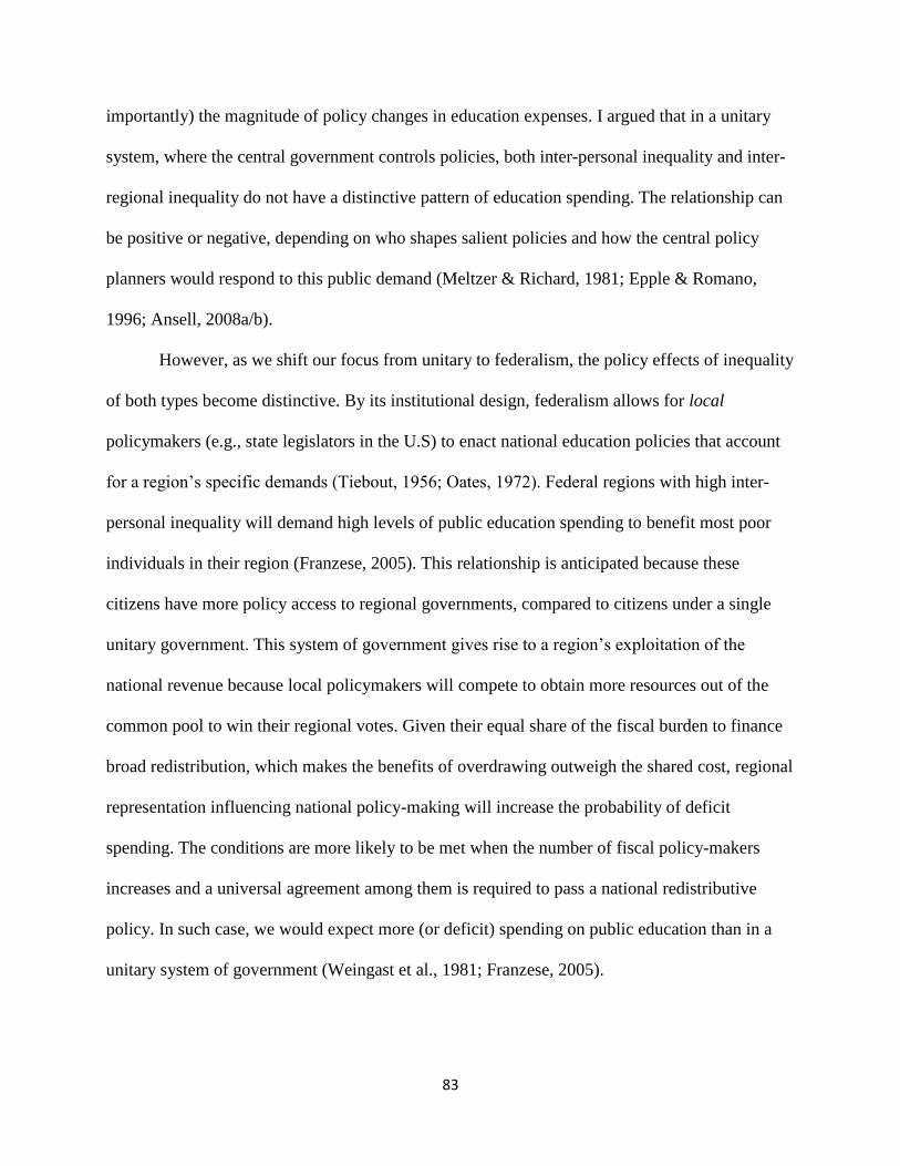
83
importantly) the magnitude of policy changes in education expenses. I argued that in a unitary
system, where the central government controls policies, both inter-personal inequality and inter-
regional inequality do not have a distinctive pattern of education spending. The relationship can
be positive or negative, depending on who shapes salient policies and how the central policy
planners would respond to this public demand (Meltzer & Richard, 1981; Epple & Romano,
1996; Ansell, 2008a/b).
However, as we shift our focus from unitary to federalism, the policy effects of inequality
of both types become distinctive. By its institutional design, federalism allows for local
policymakers (e.g., state legislators in the U.S) to enact national education policies that account
for a region’s specific demands (Tiebout, 1956; Oates, 1972). Federal regions with high inter-
personal inequality will demand high levels of public education spending to benefit most poor
individuals in their region (Franzese, 2005). This relationship is anticipated because these
citizens have more policy access to regional governments, compared to citizens under a single
unitary government. This system of government gives rise to a region’s exploitation of the
national revenue because local policymakers will compete to obtain more resources out of the
common pool to win their regional votes. Given their equal share of the fiscal burden to finance
broad redistribution, which makes the benefits of overdrawing outweigh the shared cost, regional
representation influencing national policy-making will increase the probability of deficit
spending. The conditions are more likely to be met when the number of fiscal policy-makers
increases and a universal agreement among them is required to pass a national redistributive
policy. In such case, we would expect more (or deficit) spending on public education than in a
unitary system of government (Weingast et al., 1981; Franzese, 2005).

84
In comparison, federal regions with high inter-regional inequality will find it hard to draw
a policy consensus on reforming redistribution than regions ruled by a unitary government.
Under a federal system, national policy making power is diffused equally to both rich and poor
regions.51 However, this diffusive power would work as a system of policy constraint as regional
disparity grows. For wealthy federal regions compared to the poorer counterparts, broader
redistribution creates a larger fiscal burden. Thus, national delegates from these richer regions
will seek to block fiscal expansion and pass budget cuts to redistributive spending. Poor regions
also have veto power to delay budget cuts while this tool is not useful to expand spending. As
regional inequality increases, the coordination of policy decision making between the rich and
the poor regions will become increasingly difficult, leading to a stalemate in which policy
gridlock is anticipated (Weingast et al., 1981; Giuranno, 2009a/b; Tsebelis, 2002; Triesman,
2000).
In hypothesis testing, I expect two possible outcomes regarding the level and magnitude
of public education spending. A federal system with inter-personal inequality, further increases
the level of public education spending, relative to a unitary system of government. On the other
hand, a federal system with inter-regional inequality engenders less change (irrespective of an
increase or decrease) in reforming public education spending than a unitary system of
government.
Data
To test the policy effects incurred by the joint relationship between income inequality and
51 Recognizing that regions’ powers can differ in federations depending on, among other things, malapportionment,
and population distributions.

85
federalism across countries over time, I use the panel data from 18 OECD countries from 1980 to
2010. My choice of the OECD data is based on the availability of regional inequality measures
as well as refined institutional controls to be used in the estimated models.
Dependent Variable
To gauge the size of overall public education spending weighted by the size of national
economies, I use the general government’s expenditure on public education as a share of GDP.
Public education spending at the general government level includes all levels of human capital
investment (primary, secondary, tertiary, and others). The general government spending measure
is also applied to both a unitary system of government and federalism to capture overall flows of
redistribution better. The intent is partly because the redistribution would not be fully captured
from a scope of the central government finance if regions have strong incentive to isolate their
fiscal sources. This data series is available from the World Development Indicators (WDI)
database provided by the World Bank group. I used public education spending observations for
18 OECD countries from 1980 through 2010.
Measures of Inter-personal Inequality
The distribution of individual income inequality is measured in the ratio of individual
earnings in the upper 90th percentile to earnings in the bottom 10th percentile – I call this
P9010.52 Although Gini coefficients are another popular measure used in the literature, Gini
52 As an alternative measure, I use the decomposition of P9010 - income differentials in the two halves of the
individual income distribution based on the 90th – 50th earnings ratio divided by the 50th – 10th earnings ratio. This
alternative measure is useful to know what extent the P9010 ratio is driven by inequality in the top of distribution

86
Table 7. Education Spending (GDP %) and Structure of Inequality in 18 OECD Countries
Average Values from 1980 to 2010
(Sources: OECD Stat 2007; Lupe and
Pontusson 2011; World Development
Indicators; UNESCO Institute for
Statistics; the author’s calculation)
90-10 Ratio
Gini
COV
GDP (%)
Countries
P9010
Ratio
Gini
(%)
COV
(0-1)
GDP
(%) Min Max Min Max Min Max
Min Max
Austria 3.31 (9) 32.47 0.22 (6) 5.45 3.23 3.38 29.00 34.60 0.19 0.24 5.01 6.25
Belgium 2.36 (16) 27.54 0.38 (1) 5.41 2.25 2.49 22.70 37.47 0.35 0.42 3.03 6.44
Canada 3.96 (3) 34.88 0.28 (3) 6.17 3.52 4.45 30.51 37.20 0.20 0.37 4.77 7.88
Denmark 2.39 (14) 29.70 0.16 (16) 7.56 2.14 2.74 27.26 32.10 0.14 0.18 5.70 8.72
Finland 2.45 (13) 21.97 0.21 (8) 5.93 2.29 2.59 15.05 25.86 0.14 0.26 4.77 7.65
France 3.11 (10) 27.72 0.18 (15) 5.30 2.83 3.28 23.98 29.20 0.16 0.19 4.38 5.90
Germany 3.34 (8) 24.12 0.30 (2) 4.53 2.94 4.28 19.89 26.60 0.25 0.43 4.43 4.61
Greece 3.36 (7) 24.35 0.21 (9) 2.62 3.24 3.44 21.80 27.20 0.16 0.28 1.77 4.09
Ireland 3.77 (4) 27.38 0.20 (10) 5.01 3.26 4.06 24.40 30.26 0.12 0.26 4.22 5.91
Italy 2.37 (15) 32.93 0.25 (4) 4.62 2.22 2.60 31.23 34.90 0.23 0.27 3.95 4.96
Netherlands 2.68 (11) 32.24 0.19 (13) 5.52 2.40 2.92 29.32 33.60 0.12 0.38 4.84 6.37
Norway 2.12 (18) 22.01 0.20 (11) 6.68 1.95 2.29 19.70 25.20 0.14 0.27 5.35 7.99
Portugal 4.36 (2) 23.42 0.24 (5) 4.33 4.25 4.66 22.19 25.60 0.19 0.36 3.09 5.79
Spain 3.70 (5) 22.80 0.19 (14) 4.21 3.29 4.22 20.81 25.54 0.18 0.23 3.22 4.98
Sweden 2.17 (17) 22.96 0.13 (18) 6.79 1.95 2.35 16.82 25.00 0.08 0.17 5.56 7.51
Switzerland 2.58 (12) 29.71 0.16 (17) 5.17 2.42 2.69 26.80 31.26 0.14 0.19 4.62 6.00
UK 3.40 (6) 31.40 0.20 (12) 5.01 2.98 3.64 25.85 35.30 0.16 0.23 4.37 5.63
USA 4.46 (1) 32.61 0.22 (7) 5.27 3.78 5.02 26.88 36.54 0.16 0.46 4.76 5.77
Note: Values in parentheses are country ranking.
vis-à-vis inequality at the bottom. As put forth by Lupe and Pontusson (2011), this method is designed to capture a
type of SKEW in the 90th -50th earnings ratio over the 50th – 10th earnings ratio. The degree of SKEW is important
because when the distance between the middle income and the lower-income is smaller relative to the distance
between the middle income and the upper-middle, the middle-income voters could “empathize” with the poorer and
support redistributive policies (in the absence of cross-cutting ethnic cleavages). Otherwise, such redistributive
motives will be a minor concern under a higher level of SKEW.

87
coefficients take account of the full income distribution identified as the relationship of
cumulative shares of the entire national income received by the population. The income quintile
ratios are preferred in my research because I am interested in the gap between the poor and the
rich. The income quintile ratio is also easy to interpret. Take for an example that the P9010 ratio
is equal to 5 (see Appendix 8 for the data ranges from 1.95 to 5.02 for the OECD samples). It
means that the poorest person in the richest 10 percent of the population in the income
distribution earns five times as much income as the richest person in the poorest 10 percent
would earn. Table 7 (above) shows time-series cross-national comparison for the distribution of
P9010. The United States, compared with Norway (ranked in the lowest in P9010), has a P9010
ratio difference of 4.46 to 2.12. That says, for example, in US dollar terms, the poorest person in
the richest group makes about four dollars more on average, compared to every single dollar that
the richest of the poorest group makes. However, in Norwegian Krone, the poorest of the richest
group makes about two Krones more. The income quintile ratio data are available from the
OECD Statistics database.
Measures of Inter-regional Inequality
Measuring regional disparity is difficult because the subnational unit level data is limited
and internationally comparable measures of geographic distribution of wealth to a country
require the consideration of many contingent factors. Empirical studies of OECD countries have
displayed a relative success in the data collection and use for robust inequality measures (Kessler
& Lessmann, 2010; Lessmann, 2009, 2011). These macro data relates regional GDP per capita,
the country’s average GDP per capita, the share of the country’s total population in a region, and
the number of regions in that country. From research on subnational income level data, regional

88
GDP per capita data is obtainable from the Cambridge Econometrics Database. I adopt a
mathematical formula most popularly used for calculating regional disparity (Lessmann, 2009,
p.2460): the coefficient of variations of regional GDP per capita (COV).53
53 I also calculated for two alternative measures for robustness (Lessmann, 2009): 1) the population-weighted
coefficient of variation (COVW) = 1
�̅�√
1
𝑛∑ 𝑝𝑖(�̅� − 𝑦𝑖)2𝑛
𝑖=1 , 2) the adjusted Gini coefficient (ADGINI)
= 2 ∑ 𝑖𝑦𝑖
𝑛𝑖=1
𝑛 ∑ 𝑖𝑦𝑖𝑛𝑖=1
−𝑛
𝑛−1 . I emphasize that three disparity measures (COV, COVW, ADGINI) are conceptually different
from each other. While both COV and COVW are measures of dispersion, COVW differs slightly by having values
adjusted for the share of the country population in a region. It could be possible for a measure of COV, without
taking different population densities into account, to report a high score, while COV may not actually matter to a lot
of people. For example, one region with 1,000 inhabitants and a regional GDP per capita of $20,000; the second
region has a regional GDP per capita of $10,000 but only 10 inhabitants (Lessmann, 2006).
Compared to COV and COVW, ADGINI focuses more on measuring deprivation. Dispersion and
deprivation are two ways to conceptualize spatial differences in wealth (see Protnove & Felsenten, 2005). The
dispersion measures, COV and COVW, only capture the distribution of income. The ADGINI retains more
meaningful information about the extent of relative poverty, not merely income spread. In ADGINI, additional
weight is given to a region’s wealth as it veers farther away from the mean of the inter-regional regional wealth
distribution. This weight value makes the inequality measure more sensitive to changes in the upper or lower tail of
this distribution.
The United States and Argentina clearly show the differences in these three measures. In the United States
in 2010, per capita income approximated USD $50,000 in Massachusetts and $30,000 in Mississippi. In Argentina
in 2006, gross provincial product per capita in Buenos Aires was USD $25, 000 and $2,500 in Tucuman. COV
would calculate these differences to be similar across jurisdictions – around $20,000. The ADGINI variable,
however, would take into account the meaningful differences in relative wealth in development is relatively even
and social safety nets redistribute wealth to the neediest populations.

89
COV = 1
�̅�√
1
𝑛∑ (�̅� − 𝑦𝑖)2𝑛
𝑖=1
where �̅� denotes the country’s average GDP per capita. 𝑦𝑖 is the GDP per capita of a region i. 𝑝𝑖
indicates the share of the country’s total population in region i. Finally, n is the number of
regions within a country. This measure is cross-nationally comparable (Lessmann, 2009; Portnov
& Felsensten, 2005).
COV is calculated based on the regional level GDP data from 18 OECD countries
covering the years from 1980 to 2010. This cross-national sample is the most available coverage
for regional GDP per capita.54 See Table 7 for the cross-national time series sample data
distribution. COV allows for the “intra-country” variance information to be translated into the
numerically continuous index (0-1) of “inter-country” variance. For inferential purposes, I
rescale these numbers on one to ten scales. The value of zero denotes that a country is perfectly
evenly developed across its regions, but the value of ten represents extreme inequality.
Two Uncorrelated Measures of Inequality
Inter-regional inequality and inter-personal inequality are not only conceptually
independent but also empirically uncorrelated with each other. Table 8 includes a country’s score
of inter-regional inequality (COV as a variation of regional GDP per capita). This chart also
includes a country’s score of inter-personal inequality measured in two folds: 1) Gini (in percent)
detects inequality in the distribution of aggregated individual income, 2) P90/10 (in ratio of the
54 Unfortunately, the micro-level data on economic inequality across sub-national units are not widely available for
most developing countries. They are critical for calibrating cross-nationally comparable measures of regional
disparity.

90
Table 8. Inter-regional Inequality and Inter-personal Inequality Compared
Average value from 2006 to 2010
Ranking
Inter-regional Inequality Inter-personal Inequality
Countries COV
(0-1)
Countries
Gini
(0-100) Countries
P90/10
(ratio)
1 Belgium 0.352 Canada 36.19 USA 4.92
2 Canada 0.318 USA 35.55 Portugal 4.28
3 Germany 0.307 Austria 33.00 Ireland 3.85
4 Norway 0.267 Italy 32.92 Canada 3.73
5 Greece 0.248 UK 31.81 Germany 3.62
6 Ireland 0.234 Denmark 31.75 UK 3.60
7 Italy 0.231 Netherlands 30.17 Spain 3.42
8 UK 0.225 Switzerland 30.06 Austria 3.34
9 Portugal 0.216 Ireland 29.91 Greece 3.33
10 Finland 0.201 France 28.25 Netherlands 2.90
11 France 0.192 Belgium 26.99 France 2.88
12 Austria 0.188 Greece 25.72 Denmark 2.71
13 USA 0.185 Spain 25.43 Switzerland 2.68
14 Spain 0.181 Germany 25.36 Finland 2.55
15 Switzerland 0.177 Sweden 23.49 Belgium 2.34
16 Denmark 0.172 Finland 23.45 Sweden 2.30
17 Sweden 0.156 Portugal 23.11 Italy 2.26
18 Netherlands 0.155 Norway 22.63 Norway 2.25
Note: the pairwise correlation of COV (Coefficient of Variations of regional GDP per capita) and Gini is -0.04 (p-
value = 0.88). The pairwise correlation of COV and P90/10 is 0.023 (p-value = 0.93). 1 for COV means shares of
national income by only one region. 100% for Gini means shares of national income by only one person. P90/10 is
the ratio of the 10% of people with the highest income to the 10% of people with the lowest income. For example,
USA shows 4.9 in P90/10 ratio; this means that the poorest individual of the richest group earns 4.9 times more per
every single dollar than the richest individual of the poorest group.
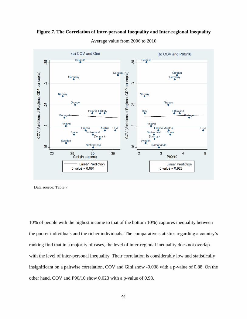
91
Figure 7. The Correlation of Inter-personal Inequality and Inter-regional Inequality
Average value from 2006 to 2010
Data source: Table 7
10% of people with the highest income to that of the bottom 10%) captures inequality between
the poorer individuals and the richer individuals. The comparative statistics regarding a country’s
ranking find that in a majority of cases, the level of inter-regional inequality does not overlap
with the level of inter-personal inequality. Their correlation is considerably low and statistically
insignificant on a pairwise correlation, COV and Gini show -0.038 with a p-value of 0.88. On the
other hand, COV and P90/10 show 0.023 with a p-value of 0.93.

92
Substantively, Belgium ranks in the middle of inter-personal inequality based on Gini
index and the bottom of inter-personal inequality based on P90/10. However, the level of inter-
regional inequality in Belgium is the highest based on COV.55 The United States is an opposite
case. Its inter-personal inequality level for both Gini and P90/10 is very high in the country
ranking.56 However, the inter-regional inequality in the United States shows a relatively equal
regional income distribution, compared with other the two-thirds of the sample from OECD
countries in the same period.
Figure 7 (above) shows the statistical relationship between inter-regional inequality and
inter-personal inequality. Again, there is no clear evidence that inter-personal inequality is
linearly correlated with inter-regional inequality. A linear prediction line for the bivariate
relationship between inter-regional inequality and inter-personal inequality finds a statistically
insignificant slope.
Measures of Federalism
I measure federalism as a political decentralization for several reasons. Most importantly,
federalism captures the political dynamics, local input in policy-making, that I argue produce
divergence across regions. Thus, measures of political decentralization would be like my
55 Lessmann (2011) reports the same concern for Belgium.
56 This is partly explained by the Congressional Budget Office’s report on income trends from 1979 to 2007. Income
grew by 18 percent of share of income for the bottom 20 percent of households, but 275 percent for the top 1 percent
of households. See http://www.cbo.gov/sites/default/files/cbofiles/attachments/10-25-HouseholdIncome.pdf

93
Table 9. Measures of Federalism
Country
Electoral Federalism (1980-2009)
Are state/province governments locally elected? (Beck et al. 2010,
Database of Political Institutions)
0 = No local election
1 = Legislature locally elected
2 = Legislature and executive locally elected
Mean St. Dev Min Max
Austria 2 0 2 2
Belgium 1.53 0.51 1 2
Canada 2 0 2 2
Denmark 2 0 2 2
Finland 0.30 0.46 0 1
France 1 0 1 1
Germany 2 0 2 2
Greece 0.87 0.35 0 1
Ireland 2 0 2 2
Italy 2 0 2 2
Netherlands 1 0 1 1
Norway 1 0 1 1
Portugal 0.15 0.53 0 2
Spain 2 0 2 2
Sweden 1 0 1 1
Switzerland 2 0 2 2
UK 2 0 2 2
USA 2 0 2 2
conceptualization of federalism. I focus on electoral federalism57 because I am interested in
capturing the level of the closeness between local politicians and their local constituencies. This
57 I use fiscal federalism as an alternative measure. Fiscal autonomy is important to the functioning of federalism.
Without money and the ability to spend it, federalism may have little policy effect. I take a veto player approach by
using a discrete index of approximate strength of regional governments’ power over the distribution of tax revenue.
The data and codebook are accessible at http://www.unc.edu/~hooghe/data_ra.php. This measure captures whether
local governments can dictate spending, negotiate spending, or even cast a veto against it. The political reality could
be more complex than mere description (Sorens, 2011). The interactive relationship between fiscal federalism and
electoral federalism also matters, because the state governors appointed by the central government cannot go free of
94
measure is classified in the strength of federalism based on the degree of local autonomy in
electoral and fiscal matters. Electoral federalism measures subnational control over the election
of local legislative and executive office. This measure is coded 0 if unitary (no local election), 1
if the legislature is locally elected, but the executive is appointed and; 2 if both the legislature
and the executive are locally elected – see Table 9 (above) for these identifiers for the sample
countries. I am not aware, at least in my OECD country sample, of cases where the legislature is
appointed while the executive is elected at the provincial or state government level. This
trichotomous measure is collected from the Database of Political Institutions.58
Controls
We need to capture the effects of open markets on human capital investment measured by
the size of public education spending at the aggregated level. To operataionlize this, the analysis
controls for both trade openness (TRADE) and capital mobility (KAOPEN). These two
globalization measures are expected to be positively correlated with the supply of skilled labor
through human capital investment (Ansell, 2008a/b). The size of total government expenditure
(GOVTEXP) can also be positively correlated with the size of public education spending. An
the central government’s redistributive policy decision, even if the local state government may hold strong fiscal
autonomy. However, this is not an issue to my data, where electorally federal countries also tend to be fiscally
federal. The fiscal federalism measure ranges from 0 to 2, where 0 is a unitary system, 1 denotes weak fiscal
federalism, and 2 indicates strong fiscal federalism.
58 I use a measure for federalism (a type of political decentralization) rather than decentralization more broadly
because the definition of decentralization lies in conceptual muddles. It shows a mixture of fiscal, administrative,
and political decentralization. See the conceptual debates in Schneider (2003) who suggests a factor analysis to
capture those three core dimensions.

95
increase in government expenditure raises the products of private capital and increase the rate of
growth (Strauss, 2001). This growth role of government expenditure will increase human capital
investment to maintain the productivity efficiency (Barro, 1990).
On the other hand, controlling for a country’s level of economic development can be
important to relating market potentials to the size of public education spending. To scale market
potentials, the model accounts for the effect of Logged GDP per capita (GPPPC(LOG)) and GDP
per capita growth (GPPC(GROWTH)). These two economic variables are used to capture the
effect of Wagner’s law. Wagner’s law posits that increasing economic development will lead to
an increased preference for public good redistribution due to social, administrative, and welfare
issues which increase in needs and complexity (see Wagner, 1883; Castles, 1989; Busemeyer,
2007). For measuring the leftist parties’ participation in government, I use the leftist party’s
seats as a share of total legislative seats (LEFT) to capture the constituency effect directly. The
government participation by leftist parties is positively correlated with public education
spending, since their core constituencies, unskilled and poor individual voters, support broader
access to public education (Ansell, 2008a/b; Busemeyer, 2009). Lastly, to isolate demographic
pressures on the expansion of public education spending, the size of the population under age 14
(POP14) is included. The young population has a positive impact on public education spending
due to their potential demands (Busemeyer 2007). Data sources and detail descriptions are
available in Appendix 8.
Models, Methods, & Empirical Findings
Model 1 (without an Interaction Variable):

96
Public Education Spendingit = β1 Inter-personal Inequalityit + β2 Inter-regional Inequalityit
+ β3 federalism it + ∑ βjControlsit + ∑ 𝛽𝑘 Country ki + Ԑ it
𝛽𝑠 are parameter estimates. The subscript i and t are the country and year of the observations
respectively. The j and k (18) denotes, respectively, the control variable and country dummies.
The constant term is suppressed to identify the equation.
The data covers a pooled time series from 1980 to 2010. Given the data’s cross-sectional
structures (TSCS), I examine the effects of inequality on education spending across countries
over time. Despite its inferential advantages like so, the TSCS design tends to violate the
assumptions of linear regression models, such as non-constant error variance, contemporaneous
cross-sectional correlation, panel-corrected standard errors (Beck & Katz, 1995).59 My
estimation relies on panel error adjusted with AR(1) to remove serial autocorrelation.60 While
other studies of education spending use a lagged dependent variable (Busemeyer, 2007, 2009),
other authors such as Achen (2000) and Plümper et al. (2005) assess a lagged dependent variable
biases significantly downward other independent variables in the model. Their alternative
suggestion is a use of AR(1) process. Country dummies are included in the model to control
unmeasured country-specific effects such as social spending related political culture.
59 The conventional feasible generalized least squares-based algorithm (FGSL) is not appropriate to the unbalanced
panel data that we have. In our dataset, the cross-national dimensions (N=18) are smaller than the time dimension
(T=30). This condition (T>N) meets a requirement for the finite sample properties of PCSE estimators to produce
the large time asymptotic based standard errors.
60 Robustness testing for the model with the lagged dependent variable did not change main findings. However,
Kittel and Winter (2005) argue that when a lagged dependent variable is correlated with country dummies, its
combination with country fixed effects can increase statistic bias.

97
Table 10. Impacts of Inequality on the Size of Public Education Spending
Variables Estimates
(PCSE adjusted)
COV (Inter-regional Inequality)
-0.171***
(0.070)
P9010 (Inter-personal Inequality)
0.314***
(0.128)
Trade openness (trade % of GDP)
0.009**
(0.004)
Capital Openness (Chin-Ito Index) 0.446***
(0.062)
Government expenditure (as % of GDP) 0.320***
(0.029)
Left party legislative seats (as % total) 0.007**
(0.003)
GDP per capita (Logged) 1.709***
(0.465)
GDP per capita growth (annual %) 0.022
(0.013)
Population ages 0-14 (% of population) 0.352***
(0.053)
Electoral federalism 0 = No local election,
1 = the legislative locally elected but the executive appointed,
2 = both the legislative and the executive locally elected
-0.271
(0.275)
Number of observations 245
Countries 18
Country Fixed Effect Yes
R square 0.994
Note: Two-tailed tests for significant at *** p<0.01, ** p<0.05, * p<0.1. Errors are
corrected for panel specific AR1. The constant is suppressed.

98
Table 10 (above) presents findings of the positive relationship between inter-personal
inequality (P9010) and public education spending. See Appendix 9 for robustness tests. Inter-
regional inequality (COV) is negatively associated with public education spending. When
inter-personal inequality increases by 1 unit on 1-10 scales (this is equivalent to 10 percent of 0-1
index), there will be a cut in overall public education spending by 0.17 % of GDP. On the other
hand, if P9010 increases by a ratio of 2 (the poorest person of the richest 10 percent of the
population in the income distribution earns 2 times as much as the richest person of the poorest
10 percent would earn), this will lead to an increase in overall public education spending by
0.6 % of GDP (0.314*2 = 0.628). Federalism as a control of a degree of political decentralization
does not show a strong and meaningfully significant effect on overall public education spending
as mixed results presented by previous empirical studies on the policy effects of federalism show
(Martinez-Vazquez & McNab, 2003; Prud’homme, 1995; Woller & Phillips, 1998).
The effects of control variables are mostly significant with positive signs. Two economic
openness measures (trade flows and a degree of capital mobility) have positive associations with
human capital investment. The effect size of trade openness is considerably small, but this is due
to a scaling matter, given trade openness ranges from 17% to 183% of GDP. On the other hand, a
unit increase in the index of capital openness (with a sample range from -1.86 to 2.46 (more
open)) shows 0.4% of GDP. The size of government expenditure is positively associated with
public education spending. The leftist partisan power in the national legislature has positive
impact, but the effect size is relatively small compared to other economic variables (I will look
into the measured in log of GDP per capita (thousand US dollars, 2000 constant) shows that a
$100 (1% of $1000) increase in GDP per capita will lead to an increase in overall public
education spending by 1.709/100 = 0.02% of GDP. GDP per capita growth does not have a

99
significant impact on overall public education spending (I will use GDP growth as an alternative
measure). The demographic pressures measured as population age under 14 show the positive
and significant effect by a factor of 0.3% of GDP.
Model 2 (with an Interaction Variable):
Public Education Spendingit = β1 Inter-personal Inequalityit + β2 Inter-regional Inequalityit
+ β3 federalism it + β4 Inter-personal Inequality X federalism it
+ ∑ βjControlsit + ∑ 𝛽𝑘 Country ki + Ԑ it
Note: A list of controls is identical with that of Model 1. Errors are adjusted for panel corrected standard errors.
Model 2 captures the effect of inter-personal inequality on public education spending,
conditional on federalism. I measure a compound effect between inter-personal inequality and
federalism on public education spending. I obtain a marginal effect of inter-personal inequality
conditional on a degree of federalism (testing against Ho = β1 + β4 Inter-personal Inequality
*federalism it = 0). The model estimate also says the independent effect of inter-personal
inequality (β1) while holding no effect of federalism (testing against Ho = β1 = 0).
Table 11 confirms that inter-personal inequality (P9010) interacts with electoral
federalism to further increase the level of overall public education spending than with a unitary
system of government (See also Appendix 10 for robustness tests). Inter-personal inequality is
negatively, but weakly, associated with public education spending (p-value <0.1). As disused in
the theory section of Chapter 2, the effect of inter-personal inequality under a unitary system

100
Table 11. Effects of Inter-personal Inequality & Federalism
on Public Education Spending61
Estimates
Variables (PCSE adjusted)
P9010 (Inter-personal Inequality) -1.009*
(0.609)
Electoral federalism -2.042**
(0.859)
P90/10 * Electoral federalism 0.745**
(0.330)
COV (Inter-regional Inequality) -0.183***
(0.070)
Trade openness (trade % of GDP) 0.008**
(0.004)
Capital Openness (Chin-Ito Index) 0.411***
(0.068)
Government expenditure (as % of GDP) 0.298***
(0.031)
Left party legislative seats (as % total) 0.005
(0.004)
GDP per capita (Logged) 1.847***
(0.428)
GDP per capita growth (annual %) 0.019
(0.016)
Population ages 0-14 (% of population) 0.362***
(0.052)
Number of observations 245
Countries 18
Country Fixed Effect Yes
R-squared 0.994
Note: Two-tailed tests for significant at *** p<0.01, ** p<0.05, * p<0.1. Estimates are panel corrected
error adjusted with panel specific AR(1). Country fixed effects are controlled.
61 A model extension may incorporate the interaction term of federalism and COV into the estimated model.
However, this addition further complicates the role federalism, whether focusing on interpersonal inequality or inter-
regional inequality. This will be contingent upon issue salience and partisan power to the federal government.

101
Figure 8. Marginal Effect of Inter-personal Inequality (P90/10) on Public Education
Spending, Conditional on Electoral Federalism
Note: Values denote % of Public Education Spending
could be either positive or negative. However, when inter-personal inequality interacts with
federalism, there is a synergic effect of these two variables in a positive causal direction for the
size of public education spending. This synergy is anticipated in theory that federalism by nature
of its institutional design reduces a relative constraint of fiscal burdens imposed as economically
homogenous regions.
Figure 8 draws a marginal effect of inter-personal inequality on public education
spending as the strength of electoral federalism increases. As can be seen, if electoral federalism

102
allows for subnational regions to have the legislative locally elected, the marginal effect of inter-
personal inequality (by 1 unit), on average, will lead to an increase in public education spending
by 0.7% of GDP (-0.264 + 1.009 = 0.745). As the strength of federalism increases, the marginal
effect of inter-personal inequality on public education spending becomes statistically significant
inter-personal inequality, shows a significantly negative effect on the redistribution of public (see
vertical bars passing through the horizontal line of zero in Figure 8). To return to Table 11
(above), electoral federalism (in the absence of inter-personal inequality), which assumes no
effect of education spending. The effects of control variables reported from Table 10 remain
intact for their signs and statistical significance.
Model 3 (with an Interaction Variable)
†Public Education Spendingit = β1 Inter-personal Inequalityit + β2 Inter-regional Inequalityit
+ β3 federalism it + β4 Inter-regional Inequality X federalism it
+ ∑ βjControlsit + ∑ 𝛽𝑘 Country ki + Ԑ it
Notes: † Volatility is calculated by the standard deviation for non-overlapping three-year periods. A list of controls is
identical with that of Model 1. Errors are adjusted for panel corrected standard errors.
To test the effects of veto player constraints, I modified the dependent variable by taking the
standard deviation of non-overlapping three-year periods from 1980 to 2010 The standard
deviation serves to measure policy volatility, commonly used in the political economy literature
(Aisen & Veiga, 2005).62 Lower values mean less change (i.e., a higher likelihood of
62 I also used non-overlapping 5 year-periods for alternative standard deviation calculations and found the key
variable effects remain largely intact.

103
perpetuating policy gridlock) while higher values are more change (i.e., a lower likelihood of
policy gridlock). According to veto player constraints, we should expect to see lower values.
Model 3 uses the standard deviation of public education spending on the left-hand side. The
average values of three years for independent variables are used on the right-hand side of Model
3. One exception is made because a degree of federalism is discrete, so I took the maximum level
during three years and coded it as individual observation used in Model 3.
Based on results from Table 12, inter-regional inequality interacts with federalism to
dampen the volatility of public education spending – see Appendix 11 for robustness tests. Note
that the coefficient of the electoral federalism’s independent effect is positive (more changes)
when assuming regions are fairly identical in comparison. However, in conditional hypothesis
testing, inter-regional inequality (in the absence of federalism effects) has a positive effect on the
volatility of public education spending because inter-regional inequality could either increase or
decrease the level of public education spending. However, inter-regional inequality and
federalism produce a synergic effect of reducing the change in public education spending.
Figure 9 presents the marginal effect of inter-regional inequality (COV) on volatility in
the size of public education spending. As a degree of federalism increases, the marginal effect of
inter-personal inequality, on average, dampens significantly: a shift from a unitary system of
government with no local election to weak federalism with the legislative locally elected will
lead to 0.25 standard deviation less change from the three-year average of public education
spending (0.088 – 0.347 = - 0.25). When a country shifts from a unitary system of government
to adopt a system of full-blown federalism (regarding electoral federalism), the marginal effect
of inter-personal inequality, on average, will reduce changes by a 0.518 deviation from the three-

104
Table 12. Effects of Economic Inequality & Federalism
on Volatility of Public Education Spending†
Estimates
Variables (PCSE adjusted)
COV (Inter-regional Inequality) 0.347***
(0.068)
Electoral federalism 0.443**
(0.173)
COV * Electoral federalism -0.259***
(0.052)
P9010 (Inter-personal Inequality) 0.264***
(0.069)
Trade openness (trade % of GDP) -0.002
(0.002)
Capital Openness (Chin-Ito Index) -0.008
(0.029)
Government expenditure (as % of GDP) 0.036**
(0.016)
Left party legislative seats (as % total) 0.005**
(0.002)
GDP per capita (Logged) -0.220
(0.177)
GDP per capita growth (annual %) -0.025**
(0.012)
Population ages 0-14 (% of population) -0.048***
(0.018)
Number of observations 91
Countries 18
Country Fixed Effect Yes
R-squared 0.879
Note: Two-tailed tests for significant at *** p<0.01, ** p<0.05, * p<0.1. Estimates are panel corrected error
adjusted based on lagged dependent variable models. Country fixed effects are controlled. †Volatility is the
standard deviation of government expenditure on public education over three years non-overlapping periods
between 1980 and 2010. †† Values are taken for the maximum score during three years; all other
independent variables take the average value of three years.

105
Figure 9. Marginal Effect of Inter-regional Inequality (COV) on Volatility of Public
Education Spending, Conditional on Electoral Federalism
Note; Values denote the standard deviation from average public education spending
year average of public education spending (-0.171-0347 = - 0.518). This conditional dampening
effect of inter-regional inequality under federalism is statistically significant.
In return to Table 12 (above), the sign of coefficients for each control variable can be
read regarding more change or less change. Inter-personal inequality (P9010) creates more
changes because the effect could be positive or negative on redistribution. The oversized
government expenditure is positively correlated with more volatility since it will create upward

106
pressures on public education spending. The effect of left party power creates upward pressure
for the size of public education spending because the core constituencies of the left prefer the
broad distribution of public education spending (Stasavage, 2005; Ansell, 2008a/b; Boix, 1995;
Buesmeyer, 2007). For GDP per capita growth, I suspect that economic growth is endogenously
related with the volatility of government spending. The growth literature points to negative
effects of government spending volatility on economic growth (Carmiganni et al., 2007, Fatas &
Mihov, 2003; Fuceri, 2007). Increases in the population under age 14 as a proportion of the total
is used as a proxy for demographic pressures for public education (particularly in primary
education). The effect of this variable shows less change because in OECD countries, the effect
of demographic pressures for public finance on education conflicts with the growing aging
population. See for Preston’s (1984) generational competition hypothesis; Richman and
Stagner’s (1986) extension to Preston. For example, Poterba’s (1996) panel data analysis of the
U.S. states over the 1960-1990 periods shows that an increase in the fraction of elderly residents
affects a significant reduction in per child educational spending.
Conclusion and Policy Implications
I began my inequality research by asking what the role of political geography is about the
redistribution of public education spending, focusing on the level and variability of spending
adjustment. This chapter provides evidence that the redistributive policy effect of inter-regional
inequality works differently from that of inter-personal inequality under federalism. My subset
arguments distinguish the fractionalization effects of federalism from the polarization effects of
federalism. I argue for inter-personal inequality as amplifying fractionalization effects of
federalism that exacerbate regions’ overuse of the common pool. The important prediction is

107
high levels of public education spending nationwide. Stemming from this directional
expectation, I argue that higher inter-regional inequality worsens policy conflicts between
regions bearing their unequal share of fiscal burdens to finance broad redistribution. Given this,
inter-regional inequality further amplifies the polarization effects of federalism. Applying this to
the policy effects of federalism for high inter-regional inequality, I expect that the magnitude of
changes in public education spending will be small. Using the panel data for 18 OECD countries
from 1980 to 2010, I find supporting evidence for these two conditional arguments (one for
levels and the other for the volatility).
These theoretical and empirical distinctions regarding inequality of both types (individual
focus versus regional focus), however, will entirely depend on the level of analysis as well as the
institutional structure in a country. The logical outcome of RMR (the greater the inequality, the
greater the government spending) will make sense only if examining redistributive politics
within one undifferentiated jurisdiction that has a majoritarian voting rule and a system of
progressive taxation. When there is more than one jurisdiction, the median voters’ policy
interests (suggested by RMR) will vary across multiple subnational jurisdictions. In this chapter,
I show federalism as a political structure that highlights the importance of the spatial measure of
inequality. I further acknowledge that the political geography of inequality is also important to
other institutional factors such as voting districts and district-oriented voting behavior (the
personal votes). Some institutional context will dampen the policy effects of inter-regional
inequality.
For instance, presidential systems based on a popular vote will encourage cross-regional
coalitions. In this case, nationally aggregated individual income distribution (inter-personal
inequality) will be a more politically relevant inequality measure. Another example of the utility

108
of inter-personal inequality measures can be found in the demographic context that a country is
divided into nearly homogenous regions. Wealth distribution, in this case, is similar in each
region, rendering a similar type of median voter within it.
Applying inter-regional inequality to this demographic context will be misleading in
predicting political behavior, but will also obfuscate the variance of the relevant factors of
inequality in that country. When in fact, the opposite case will be true; aggregated individual
income measures applied to where inter-regional inequality is high but inter-personal inequality
is low. Then this misapplication will lead to perplexing policy results.
When choosing more appropriate indicators of inequality, it is critical to match these
indicators with the relevant political / demographic conditions of a country. In political contexts,
we need to consider both jurisdictional representation and accountability. To address
demographic contexts, we need to look at the divergence between individual and regional
inequality.
One way to assess this divergence can be done in framing four dimensions of inequality
divergence: 1) high inter-personal & high inter-regional, 2) low inter-personal & low inter-
regional, 3) high inter-personal & low inter-regional, 4) low inter-personal & high inter-regional.
In a country that has a match on inequality of two types (as described in cases #1 and #2), the
distinctions between those two inequality indicators are of little importance and empirical
findings based on either measure will be relatively less affected by choice of inequality
measured. However, where countries have a mismatch on inequality of two types (case #3 – the
U.S.A, case #4 – Belgium, c.f. Table 8), the choice of inequality indicators will be integral.
Also, the weak association between these two inequality indicators suggests how much countries
deviate. Therefore, distinguishing the geographic measure of inequality from the aggregated

109
individual measure of inequality is theoretically, as well as empirically important to account for
policy effects.
This chapter attempts to understand policy effects subject to types of inequality under a
federal system of government. Based on the limited quality of data on inter-regional income
disparity (a cross-nationally comparable measure of the intra-country variance), this chapter is a
first step to unfold the complexity of public spending.
110
CHAPTER 5
Empirical Analysis of Policy Bargaining:
Testing the Conditional Theory of Regional Inequality and Decentralization
Previous studies show cross-national evidence that a decentralized country with uneven
regional economies tends to experience difficulties in centrally financing public goods broadly
redistributed across disparate regions. Many of these works share insights from Tsebelis’ (2002)
study of veto gates in institutional politics. This veto player research predicts a general policy
outcome: diversified regional preferences together with the power of regional authority to block
national policies are likely to create policy gridlock at the challenge of national policy
coordination.
I presented cross-national evidence that a federalist country with uneven regional
economies tends to experience greater difficulty in changing public education financing. The
higher likelihood of policy gridlock is anticipated as regional preferences become more divergent
and regional authority to block national policies further increases.
This empirical chapter, however, presents counter evidence that not all types of
redistributive spending are prone to policy gridlock. Even the redistributive spending that goes
disproportionally to poor regions can still benefit rich regions or at least minimize the latter’s
relative loss by targeting policy benefits to specific individuals within every territorial region.
Given this shared interest, poor areas which prefer centralizing more interregional (as well as
interpersonal) redistribution find it easier to achieve policy coordination with their affluent
counterparts.

111
Most importantly, this chapter highlights specific conditions under which redistributive
policy pressures from economic disparities among autonomous regions encourages a strategic
coalition between rich and poor areas to facilitate the centralized redistribution of public
spending. As an example of this condition, I point to targeted spending such as social
expenditure that directs the associated policy benefits primarily to qualified individuals rather
than to the society as a whole. Using a new annual dataset for policy priority measures
comparable across 22 OECD countries over the recent 20 years, I find supporting evidence.
Growing regional income disparity in highly decentralized countries tends to be accompanied by
growing centralized redistribution of public spending towards social policies while shifting away
from policies that can isolate policy benefits solely on a regional base.
The rest of this empirical chapter is organized as follows. First, I briefly review the
literature and theorize my institution-grounded contextual hypothesis to be tested. There, I pace
emphasis on the combined effect of variations in redistributive demands from disparate regions
and the regionalized administrative authority. The second section is dedicated to describing the
attributes of the data for regression analysis. There, I discuss data analytic strategies, followed by
explaining variables and measurement in detail. In the following section, I discuss the data
analytic results. I conclude this empirical chapter with a potential research extension and policy
implications.
Bargaining for a Centralized Provision of Public Policies
Copious studies on redistributive spending offer compelling models for how and when
redistributive pressures from the poor majority shape public policy choices. There is little

112
discussion, however, drawn from these models to help us understand redistributive spending as a
bargaining outcome between the poor majority and the rich minority.
Fortunately, a few exceptional studies are devoting their attentions to the comparative
analyses of redistributive spending elaborated from a regional perspective. For example, the
popular analysis of public spending (e.g., Meltzer-Richard model of public spending) primarily
focuses on a policy dictatorship of the poor majority where the rich are considered as politically
marginal.
Extending from this analytical tradition, Giuranno (2009a, 2009b) highlights a likelihood
of policy vetoes sought by the rich regions in a country with economically highly-disparate
regions. According to him, we should expect more policy vetoes of national legislation from the
rich regions if the central government looks to increase the tax-funded public spending that goes
disproportionately to the poor regions. Giuranno’s study offers an important insight: wealthy
individuals may be less powerful regarding democratic vote counts than their poor majority
counterparts. However, the rich regions can project their parochial interests through formal
powers allotted to territories in the making of national legislation. The rich regions are more
likely to exercise their policy vetoes when it becomes inefficient for their money to go to the
central government to be redistributed disproportionately to the poor regions. With the rise in
regional disparities, it is likely that the rich regions find the centralized format of redistributive
policies less efficient and contradictory to their strategic policy interest. Thus, policy
noncompliance will be affected by a rich region’s preference regarding the trade-offs between
equity enhancement due to broad redistribution (Tanzi, 2000) and the incentives to constrain
large redistribution due to the cost of efficiency losses (Aysen, 2005).

113
Overall, whether explicitly or implicitly, these present studies describe regional disparity
as a major obstacle to centralized policy bargaining by representatives of localities. To be
specific, regional economic disparities deepen the polarization in policy interests between the
rich and the poor jurisdictions. This divergence exacerbates interregional redistributive conflicts,
potentially leading to the under-provision of public goods and services across sub-national
regions.
This conflict model, however, understates that a policy bargain between disparate regions
can be easier under the decentralized system of regions when goods are directed to individuals
regardless of region. Consistent with works of Basley and Coate (2003) and Giuranno (2009b), I
argue for a condition under which autonomous regions with uneven regional economies achieve
policy coordination in the centralized provision of public spending. A good candidate of this
condition is a targeted spending specific to individual benefits (e.g., social security transfers and
health expenditure).
The key implication for the rich regions is that not all types of the centralized provision
of redistributive policy come at a high cost while policy goods are disproportionally redistributed
to poor regions. Implementing some policies is (relatively) less expensive than others when cost
sharing is unavoidable.63 By ensuring the allocation of public money to be directed to individual
beneficiaries who are a segment of their regional population, the rich regions reduce the
efficiency loss associated with the redistributive policy. Targeted spending becomes a significant
63 The main reasons these costs might be unavoidable are due to externalities and migration. If poor regions become
too disparate without resources to aid their impoverished citizens, the poor in the poor regions are likely to move to
the richer regions. Moreover, rich regions may have economic risks against which they would want to share the
burden of social insurance with poorer regions (Beramendi, 2012).

114
policy preference for the representatives of the rich regions as they seek to win an electoral
support from their local voters. Moreover, in the existence of logrolling institutions to facilitate
political exchange, the affluent regions will have a stronger incentive to coordinate this
centralized provision of targeted spending policy with the poor regions.
On the other hand, my argument for the poor regions implies that more targeted spending
is a desirable policy option because it creates positive spillover effects which contribute to the
general welfare of the poor majority within a local district. Since individual beneficiaries in poor
regions outnumber those in rich regions, a centralized policy provision of target spending agreed
by the rich regions should also be in the poor regions’ best interest. This regional interest
becomes stronger the poorer the regions are. It will create an easy bargaining situation. The
compromise between the interests of the rich and the poor regions is likely to engender a
reasonable policy change.64
In short, a high level of legislative conflict among economically disparate regions does
not necessarily escalate all types of tax-funded public spending programs into policy gridlock.
Instead, targeted spending programs may be more conducive to policy agreement than non-
targeted ones; that is, regions are likely to reach a pro-spending agreement on programs specific
to individuals. This policy outcome is probably with countries that have economically highly-
disparate regions and diffuse policy authority across their territorial regions to a greater extent.
Based on this argument, I predict a testable hypothesis for the growth of social spending
in a decentralized country with growing regional inequality. In data analytic section below, I
focus on the combined (interaction) effects of regional disparity and decentralization rather than
64 In this case, it would be an intersubjective understanding that the autonomous rich regions are likely to attempt to
block a radical policy change during negotiating the centralized provision of redistributive policy.

115
these two variables separately. I did this to capture a bargaining condition mutually recognized
by all participants regarding demands for redistributive goods (explained by the rise of regional
disparity) injunction with local capabilities to block policy enactment at the centralized
legislation (explored by the strength of regional authority).
Data and Methodology
To conduct my contextual hypothesis testing against social spending across countries
over a reasonably extended period, I use the cross-national time-series data. This set up allows
me to capture country-level differences in their policy commitment to targeted spending. The
term “policy commitment” is operationalized in two specific ways: 1) how much is spent on
targeted policy programs, 2) how spending itself is divided across competitive policy areas. The
first definition is related to changes in a GDP share. The second definition is directly concerned
with shifts in the government’s relative policy priority from non-targeted spending programs
(geographically isolated) to targeted spending programs (specific to qualified individuals across
regions).
Measuring a country’s policy priority is challenging especially for a cross-national
analysis, partly because it needs to capture the inherent trade-offs in spending choices by nations.
The scope of the associated data is also limited in their public access. The data scope for a policy
priority analysis requires complete information on government policy spending subcategories
that are cross-nationally comparable to each other. This data constraint sets my research scope

116
for 22 OECD nations over 20 years (1990-2010) due to the availability of data across all nine
common policy areas of redistribution.65
Statistical Model Specifications
To address the empirical relationship between economic inequality across autonomous
regions and targeted spending, I use a series of error correction models (ECMs). In each model,
the dependent variable is expressed as the first difference (∆ targeted spending). This change
expression is also applied to the independent variables (except dummies) along with the level
values of these variables. My motivation for an ECM setup lies in capturing transitory policy
adjustment effects primarily. When the independent variables change in the model, the
dependent variables will adjust. The ECM estimation technique can be useful to capture both
transitory adjustment effects and enduring effects of changes in the dependent variable and allow
us to identify these two effects separately. I focus on transitory adjustment effects (noted by the
delta) rather than enduring effects (indicated by the t-1) to capture how policy (or economy)
shock will deliver effects on government spending in the short run while any significant
transitory adjustment may not be identifiable over time. My ECM model, similar to Kwon and
Pontusson (201), setup takes the following baseline form:
∆𝑦𝑖𝑡 = 𝜃𝑦𝑖𝑡 + ∑ 𝛽𝑗𝑋𝑖𝑡−1 + ∑ 𝛾𝑗∆𝑋𝑖𝑡 + 𝜀it
65 For a longer period to establish a reasonable country estimate, I use social expenditure data as an alternative proxy
for targeted spending. The data covers years from 1980 to 2010 across 26 OECD countries.

117
where ∆𝑦it indicates a change from previous year’s targeted spending (i.e., social spending as a
share of GDP or a policy priority score) in country i. X is a list of the independent variables
including income inequality indicators and socio-economic controls. Ԑ is the disturbance term. γ
is an estimated effect of transitory adjustment in the dependent variable (∆𝑦it). The long run
effect caused by one unit increase in the independent variable 𝑋𝑖𝑡−1 can be estimated by dividing
-𝛽𝑗 by the error correction rate 𝜃 (i.e., the coefficient estimate of the lagged level dependent
variable 𝑦it). My estimates of ECM models are based on the fixed effect model estimation with
the robust standard error adjusted. Fixed effects can greatly reduce omitted variable bias such
unmodeled country-specific factors as political and institutional history. Since I use the panel
data structure, I control for the heteroskedastic errors in the model estimates.
Dependent Variables
A country’s policy commitment to targeted spending can be measured by changes in
social spending or changes in policy priorities on a relative policy focus ranging from
particularized benefits and collective goods (see for a sample summary in Appendix 13 from
1980 to 2010). Public spending is often called “social” when its policy objectives serve “the
provision by public and private institutions of benefits to, and financial contributions targeted at,
households and individuals in order to provide support during circumstances which adversely
affect their welfare” (Adema et al., 2011, p.89). This policy delivery varies across (and within)
countries over time.
Figure 10 (below) plots the volatility of social expenditures across 34 OECD countries
from 1980 to 2014. Each bar graph per country indicates the range between positive and
negative year-to-year changes in social expenditure over time. The graph shows that Slovenia

118
Figure 10. Volatility of Social Expenditure across 34 OECD Countries from 1980 to 2014
Mex
ico
Isra
elK
ore
a* N
ew Z
eala
nd
* A
ust
rali
a* H
ungar
y* S
wit
zerl
and
Chil
e*(€
) It
aly
* U
nit
ed S
tate
sT
urk
ey*(€
) A
ust
ria
*(€
) G
reec
e*(€
) N
ether
lands
OE
CD
- T
ota
l* J
apan
* U
nit
ed K
ingdom
* C
anad
a*(€
) B
elgiu
m* C
zech
Rep
ubli
c*(€
) P
ort
ugal
(€)
Lux
embourg
*(€
) G
erm
any
Icel
and
*(€
) S
lovak
Rep
ubli
c*(€
) F
rance
*' N
orw
ay*(€
) S
pai
n* D
enm
ark
* S
wed
en(€
) E
stonia
*(€
) Ir
elan
d*(€
) F
inla
nd
* P
ola
nd
* S
loven
ia
Yea
r-to
-yea
r C
han
ge
in S
oci
al E
xpen
dit
ure
(%
GD
P)
-5
0
5
10
15
20
Decrease
Increase
Notes: The data is obtained from the OECD Social Expenditure Database (SCOX). Social expenditure is the sum of
government spending covering main policy areas such as old age, survivors, incapacity-related benefits, health,
family, active labor market programs, unemployment, housing, and other social policies. *(€) denotes the Eurozone
sample data used in the analysis, determined by the data availability based on model specifications using 26
countries from 1980 to 2010. The model estimates omitting Slovenia are available in the results from a panel
jackknife test available in Appendix 20.
experienced the most drastic change in the profile of social spending. For instance, between 1995
and 1996 with the inception of the accommodation to the European Monetary Union, social
spending in Slovenia increased by a GDP share of 16.5%. This number is a stark contrast to the

119
Mexican experience. For Mexico, on the other hand, the average change in social spending
between 1985 and 2012 was only about 0.22% in GDP proportion. This variation suggests
different policy efforts sought by countries to move away from the status quo spending. Figure
10 also confers a country’s relative rigidity to change the policy design of social spending. As
shown in this bar chart, the size of a bar above the zero line (welfare expansion) is bigger than
that below the zero line (welfare retrenchment). This result suggests that at the centralized
legislation of local representatives, reductions in welfare policy are harder to negotiate than
welfare increases (Obinger et al., 2005).
I use a GDP share measure of social expenditure at the general government level. The
validity of spending measure at the general government level may be threatened by
heterogeneous policy interests created in the system of multi-tier governance. Nonetheless, the
general government level data captures overall flows of cross-regional redistribution explicitly.
These flows are often intractable from an analysis of redistributive spending solely by the central
government because fiscally autonomous regions have incentives to isolate their tax revenue
from the central government. The panel data are available from the OECD Social Expenditure
Database (SCOX).66
Not only is social spending significant as a single component of the policy process, but its
relationship with other policies is important as a relative component of the resource allocation
process. Typically, the research on inequality measures relevant government expenditure as
social spending – the summation of specific government spending categories thought to be
particularly redistributive, as a percentage of GDP (Lupe & Pontusson, 2011; Beramendi &
66 For a robustness check, I also used the Global Finance Statistics (GFS) data for the central government spending
on social polies, separated from the general government. The result is reported in Appendix 17.

120
Cusack 2009; Bradley et al. 2003a; Iversen & Soskice 2006a/b; Moene & Wallerstein 2001).
These categories normally include disability benefits, survivor pensions, health benefits, family
services & family income support, housing assistance, unemployment benefits, and job market
assistances.67 However, government spending is not only structured as social spending or
otherwise, but can be broadly conceptualized by the relative scope of its reach. Many policies
related to social protection, for example, are more targeted at specific segments of the
population, while other policies, such as public order and safety, by the nature of their services,
are more broadly consumed for the entire society.68
One of the innovations of my empirical research is to analyze a complete picture of
government spending by employing a model capturing relative weights across different policy
areas known as policy priority scores (Jacoby & Schneider, 2009). Policy priorities are defined
as the component of government decision-making in which public officials allocate scarce
67 For types of social spending broken down to explicit categories (in both cash and accrual accounts), see the
aggregated dataset available from OECD Social Expenditure Statistics.
68 Every public policy program is designed for both individualistic benefits and collective benefits for the society.
However, the government’s relative emphasis differs across these policy programs. Roughly speaking, there may be
a country spending large amount on a social policy program. However, this does not necessarily mean that the
government is strongly committed to social spending. It could be that this country has a large public sector.
However, across different public policy programs, this amount of social spending could be relatively smaller than
other areas. For instance, according to the most recent 5 year average GDP share of social expenditure in Greece and
Hungary between 2007 and 2011, the level of social expenditure for these two countries was higher than the OECD
average (23 % vs. 21%). However, when considered in percentage of the total government expenditure, these
countries’ policy commitment to social expenditure was lower than the OECD average (46% vs. 48%). As
illustrated in this example, we will need to consider both the allocation of spending and the level of spending
together if addressing the country’s commitment to social spending.

121
resources, in the form of expenditure, to different program areas. The focal point does not lie just
on the question of how much a country spends on a policy program per se, but also on the
question of how a country divides up its available pool of resources. To implement this
allocation idea, I depart from restricting my analysis to the social spending variable alone.
Instead, I employ the full range of government spending to reveal policy priorities. In doing so, I
can avoid an assumption that large spending on social policies implies a policy commitment to
that area. We cannot, for example, distinguish governments with high levels of spending on all
policy areas including social spending, from those specifically dedicating resources to social
spending.
Measuring policy priorities also helps us evaluate whether countries spend in more
“particularized” (individualistic) ways or more “collective” ways as non-targeted provisions for
everyone within a region (Baron & Ferejohn 1989; Huber & Stephen 2001; Jacoby & Schneider
2001; Kousser 2005; Volden & Wiseman, 2007). The particularized way could be viewed as
targeted provision for qualified individuals across regions while the collective way could be
thought as non-targeted provision for everyone within a region. For example, social expenditures
such as health care and social protection are often categorized as particularized or individualistic
benefits because they are allocated primarily to individuals or households based on need
assessment. On the other hand, examples of collective goods are capital expenditures on
infrastructure, defense, and security that are not easily targetable to individuals but are broadly
consumed by the entire society.69 In many cases, the diffusion of public policy benefits relevant
to this non-targeted provision can be geographically isolated.
69 As pointed out by Jacoby & Schneider (2009), differentiating collective goods from particularized
(individualistic) benefits based on their policy objectives is a merely descriptive purpose. In fact, all forms of

122
Measuring of policy outputs that overcome this assessment limitation can be
operationalized by implementing a technique of the “unfolding” analysis (Coombs, 1964; Poole,
1984; Jacoby & Schneider, 2009).70 What this unfolding technique does is, rather than isolating
spending categories, it uses all government spending to “construct a geometric model in which
yearly [country] spending on policies is represented as distances between points within a space”
(Jacoby & Schneider, 2009, p.1). In other words, the unfolding technique separates policy areas
that are least likely to occur together. As a concrete example from the U.S. results (Jacoby &
Schneider, 2009), states that spend a higher percentage of their resources on law enforcement are
likely to spend a low percentage on healthcare. At the very least, this spatial proximity model
provides a yearly score for each sample country, which accurately summarizes that country’s
expenditures across all major program areas and explicitly depicts the tradeoffs that countries
make in allocating resources across program areas. Therefore, it can be interpreted as an
empirical representation of the country’s spending priorities.
Note that these spending categories have not typically been examined in studies of
inequality, apart from their contribution to total expenditures. However, this omission can be
problematic when taking into account a policy trade-off (or relative policy position): for instance,
the country which spends more on particularized benefits invariably spend less on collective
goods and vice versa (Jacoby & Schneider, 2009). The isolation of social expenditure from other
policies share the features of both collective goods and particularized benefits to a certain extent. However, in this
chapter, I use the distinction between collective goods and particularized benefits as a way to identify comparable
subsets of policies revealed in the output of unfolding analysis (see Figure 2).
70 This technique is called “unfolding” because we seek to “unfold” a country’s profiles of spending values in order
to find the relative position of the country as well as its policy point simultaneously across all countries.

123
types of public spending may thus lead to an ad-hoc or inaccurate assessment of redistributive
policies in a particular nation. Thereby, they may result in precluding the examination of the true
effects of inequality on public expenditures.
Fortunately, measuring of policy outputs that overcome this assessment limitation can be
operationalized by implementing a technique of the “unfolding” analysis (Coombs, 1964; Poole,
1984, Jacoby & Schneider, 2009).71 What this unfolding technique does is that rather than
isolating spending categories, it uses all government spending to “construct a geometric model in
which yearly [country] spending on policies is represented as distances between points within a
space” (Jacoby & Schneider, 2009, p.1). In other words, the unfolding technique separates policy
areas that are least likely to occur together.
As a concrete example from the U.S. results (Jacoby & Schneider, 2009), states that
spend a higher percentage of their resources on law enforcement are likely to spend a low
percentage on healthcare. At the very least, this spatial proximity model provides a yearly score
for each sample country, which accurately summarizes that government expenditures across all
the main program areas and explicitly depicts the tradeoffs that countries make in allocating
resources across program areas. Therefore, it can be interpreted as an empirical representation of
the country’s spending priorities.
To provide a cleaner picture of government spending in the countries of interest, I
replicate this unfolding technique using spending data from 24 OECD countries between1990
and 2010.72 To reflect a full range of policy expenditures, I used all of the expense categories
71 This technique is called “unfolding” because we seek to “unfold” a country’s profiles of spending values in order
to find the relative position of the country as well as its policy point simultaneously across all countries.
72 Complete policy spending categories for post-1960s OECD members are not available until 1990.

124
specified by the international standard Classifications of Functions of Government (COFOG).
The COFOG data allows for an unfolding technique to cover the range of ten policy areas
simultaneously: 1) general public services; 2) defense, 3) public order & safety, 4) economic
affairs, 5) environment protection, 6) housing & community amenities, 7) health, 8) recreation,
culture, & religion, 9) education, and 10) social protection. I combined the fifth and the sixth
categories together since both categories take up a very small portion of country spending (less
than 2% of the total government spending), and they are highly correlated with each other
(p<0.05). In general, the data shows the relatively small fraction of total expenditure goes to the
environment protection policy. I also ensured that spending data on those ten policy areas were
collected at the central government level. This is because the central government is the locus of
government decision making for the efficient allocation of scarce resources. Policy priorities are
outputs of a bargaining among local representatives in the national legislature.
Figure 11 below displays two outcomes of the unfolding analysis. Policy priority scores
range from -0.5 to 1.5 for the policy point location and -0.02 to 0.05 for the country locations.
The policy point location shows a coordinate for nine policies. This coordinate indicates the
relative positions of the policy points fall roughly into two comparable subsets (particularistic
benefits vs. collective goods). The policies on the left side of the graph are policies that provide
more specific services to individuals as a segment of the population within a country.
The policies on the right-hand side of the graph place focus more on spending areas for
generic regulatory purposes or the benefits of the entire society. The country mean policy
coordinates, on the other hand, show the country’s relative policy emphasis given a year.
Negative values on country scores suggest relatively more spending on policies identified on the
left side of the policy plot in Figure 11. Positive country scores indicate relatively more

125
Figure 11. An OECD Spending Data Replication for Unfolding Analysis
Notes: The scale of the illustration differs across the two dot plots. Dots on the right panel are obtained from the unfolding analysis of 24 OECD countries over
recent two decades (1990-2010). Dots on the left panel are the mean points of spending policy priorities for each country. Horizontal bars show the minimum-
maximum range of point coordinates of policy priorities for each country during the period.

126
spending identified on the right side. I interpret these scores as follows: for example, the scale
score for Germany is 0.02 unit smaller than the score for Belgium. This number means that
Germany dedicated on average 2% more of its total spending towards particularized
(individualistic) benefits than Belgium did. Importantly, many of the spending categories that are
typically considered redistributive spending are what I identify as socially (individualistically)
targeted spending using this technique. My expectation that unequal countries will spend more
on social allocation is therefore in alignment with much of the literature on the political effects of
inequality that have not examined regional inequality specifically.
Independent Variables
My interest lies in detecting the joint role of diversity in regional demands and strength of
the regional authority to play in changing national spending policy. This combined factor nicely
captures the complexity in regions’ strategic calculation of self-interests subject to their mutual
recognition of each other’s credible ability to cast a policy veto. It aims at capturing disparate
regions’ incentives to achieve a cooperative policymaking. This intent can be constructed by an
interaction term that involves the degree of regional disparity and the strength of regional
authority. Constructing measures of regional disparity is shown explicitly in the data analytic
section in Chapter 4. For a robustness check, I resort to three alternative measures of regional
disparity: in brief, COV (the coefficient of variance in the distribution of regional GDP per
capita), COVW (Population weighted COV), and ADGINI (the relative poverty adjusted Gini
coefficient of regional income). As a reminder, these are the measures of cross-nationally
comparable intra-country variance, which will allow me to examine how regional inequality
affects redistributive spending across countries.

127
To operationalize strength in the authority of regional governments, I use the Regional
Authority Index (RAI) prepared by Hooghe et al. (2015). The RAI is an annually-based measure
across ten dimensions classified into two domains of authority: 1) “self-rule, or the authority a
regional government exerts within its territory” (i.e., institutional depth, policy scope, fiscal
autonomy, borrowing autonomy, and representation), 2) “shared-rule, or the authority a regional
government or its representatives exerts in the country as a whole” (i.e., lawmaking, executive
control, fiscal control, borrowing control, constitutional reform). Please see Appendix 12 for
additional information on each dimension. The RAI is a single, continuous measure ranging from
centralization (0) in which the central government monopolizes decision-making authority to
decentralization (36.99 given my country samples) in which the regional governments have
extensive decision-making authority.
The RAI is a simplification, compared with other authors who differentiate among
vertical versus horizontal decentralization, or types of decentralization in regards to decision-
making, electoral, fiscal, or personnel (Treisman, 2002), or between fiscal, political, and
administrative decentralization (Schneider, 2003). However, these alternative measures are
largely equivalent with the ten dimensions used for calibrating the RAI. The (internal) validity of
the RAI is, therefore, high. Also, because this fine-grained RAI takes a continuous measure, the
RAI can capture a greater variation. More specifically, it tends to avoid or alleviate disagreement
concerns in the treatment of federal versus non-federal countries (Schackel, 2008).
Given the policy outcome variable of interest expressed in change terms, I expect the rise
of changes in regional disparity (∆ COV, ∆ COVW, or ∆ ADGINI) and regional authority (∆
RAI) to have a joint effect. They will lead to more positive changes in social spending and more
negative changes in policy priorities (this means, targeting more on individualistic benefits).

128
Controls
To isolate the combined effects of regional disparity and regional authority on targeted
spending, I use a full battery of controls that are commonly used in modeling of government
spending. First, a country with growing interpersonal income inequality, measured by changes in
the estimated Gini coefficient of household market (pre-tax, pre-transfer) income, is expected to
show more positive changes in social spending (and imply more negative changes in policy
priorities). Second, growing government participation by the leftist parties should be correlated
with more positive changes in social spending as they pursue more generous welfare spending.73
The government of the left is measured in the proportion of social democratic and other parties in
government based on their share in parliament (see the Comparative Political Data Set by
Armingeon et al., 2005). Third, the larger the economic growth, measured by changes in
Purchasing Power Parity (PPP) converted GDP per capita, the more the cut down of social
spending to remain competitive in the global markets. However, even at a tight budget
constraint, the government’s priority of social services may remain strong because of the needs
for protective actions to make sure that the specialized economy functions smoothly (Wagner’s
law of increase state spending).74 Fourth, growing openness to trade, measured by changes in
73 Lower income groups are usually seen as favoring social spending while upper income groups and capital desire
to have a limited role of government in shaping free market economies (Hibbs, 1987; Wittman, 1983; Keech, 1995).
In competing for votes, parties orient their policy programs to represent these different interests of class-defined core
political constituencies (Hibbs, 1987). Incumbent parties continue to do this in order to get reelected (Schmidt,
1996). In such, parties operate as “transmission belts” for social-political demands.
74 According to Wagner’s hypothesis on the upward trend of public funding, known as Wagner’s law of increasing
state spending, public sectors will grow as per capita income rises in the development of industrial economies
because of increasing demands for social services (Wagner, 1958; Peters, 2002).

129
GDP share of exports plus imports, is expected to induce reduced social spending because
greater trade integration elevates tax competition that constrains government resources (Ferris,
2003; Borcherding et al., 2005).75 In this race to the bottom, governments will find it difficult
without a significant tax revenue increase to pursue targeted policy solutions such as public
spending through social protection. That can shape changes in policy priorities of public
spending more towards collective goods. Fifth, dependent populations, measured in this case as
those over the age of 65, rely disproportionately on government services overall and welfare
spending in particular. Based on this, I expect a positive relationship between growth in the aged
population ratio (percentage of population over 65) and change in social spending, whereas a
negative correlation between this aged population ratio growth and policy priority score changes.
Sixth, growth in the organized strength of labor, measured by changes in the relative size of
union members to the total labor force, is expected to create a positive change in social spending.
Similarly, an increasing rate of unemployment (percentage of the total labor force) will lead to
growth in social benefits that are directed to the unemployed (e.g., Garrett & Mitchell, 2001;
Kittel & Winner, 2005; Rodrik, 1996, 1997).
I also use two additional institutional controls that are almost time-invariant. Seventh,
election studies show that to win votes, transfer payments sought by incumbents increase before
elections. In that regard, I control for election year effects. The election year dummy is used (1=
75 However, some scholars posit an alternative “compensatory” hypothesis whereby governments will seek to
mitigate job market risks through spending on social protection with greater openness to trade (Cameron, 1978;
Rodrik, 1996, 1997; Garrett, 1998; Martinez-Mongay, 2002; Shelton, 2007; Gemmell et al., 2008). Other authors
find no significant relationship between trade openness and public expenditures in OECD countries (Iversen &
Cusack, 2000; Kittel & Winner, 2005; Dreher, 2006; Dreher et al., 2008).

130
election year, 0 = non-election year) accordingly. Finally, to get into the EMU (European
Economic and Monetary Union), countries are required to stabilize their financial programs.
Thus, EMU country-years (assigned a value of 1 since the year of accession) are anticipated to
show a reduction in social spending. Both Election year and EMU dummies are omitted from the
policy priority change model due to collinearity.
Empirical Results
ECM estimates of targeted spending models provide evidence of a policy adjustment
engendered by the relationship of rising economic disparities among autonomous regions with a
pro-spending orientation towards social policies. Determined by the country-year data on social
expenditure from 26 OECD countries (1980-2010), Table 13 predicts an expected policy
outcome: growing regional inequality joint with regional autonomy tends to induce more positive
changes in social spending. The spending size with changes in the relative deprivation adjusted
Gini and RAI (∆ ADGINI*∆ RAI) is almost twice as big as the other measures of regional
disparity (∆ COV*∆ RAI or ∆ COVW*∆ RAI). The interaction effects of ∆ COVW and ∆ RAI
become less significant as a full battery of controls was included in the estimated model. It could
be that more densely populated regions are benefitting most from targeted policy spending,
whereas regions with a smaller size of the population benefit less.
To further examine the joint effects of regional disparity and regional authority from a
dynamic perspective, I use a marginal effect graph. Following Brambor et al. (2006), I create
Figure 12 (a)-(c) above that illustrate the marginal effects of ∆ regional disparity on ∆ social
spending, conditional on the range of ∆ RAI. As an illustration, the y-axis shows a range of
averaged marginal effects expected by one standard deviation increase in ∆ COV (or ∆ COVW
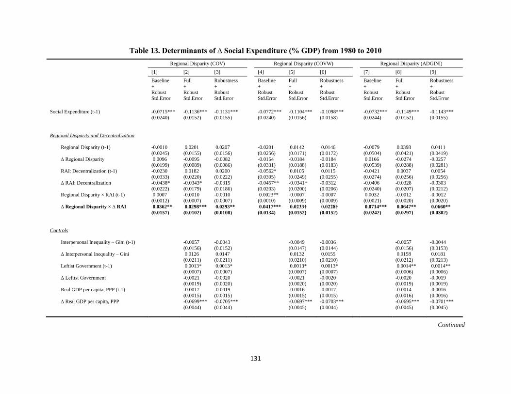
131
Table 13. Determinants of ∆ Social Expenditure (% GDP) from 1980 to 2010
Regional Disparity (COV) Regional Disparity (COVW) Regional Disparity (ADGINI)
[1] [2] [3] [4] [5] [6] [7] [8] [9]
Baseline
+ Robust
Std.Error
Full
+ Robust
Std.Error
Robustness
+ Robust
Std.Error
Baseline
+ Robust
Std.Error
Full
+ Robust
Std.Error
Robustness
+ Robust
Std.Error
Baseline
+ Robust
Std.Error
Full
+ Robust
Std.Error
Robustness
+ Robust
Std.Error
Social Expenditure (t-1) -0.0715*** -0.1136*** -0.1131*** -0.0772*** -0.1104*** -0.1098*** -0.0732*** -0.1149*** -0.1143***
(0.0240) (0.0152) (0.0155) (0.0240) (0.0156) (0.0158) (0.0244) (0.0152) (0.0155)
Regional Disparity and Decentralization
Regional Disparity (t-1) -0.0010 0.0201 0.0207 -0.0201 0.0142 0.0146 -0.0079 0.0398 0.0411
(0.0245) (0.0155) (0.0156) (0.0256) (0.0171) (0.0172) (0.0504) (0.0421) (0.0419)
∆ Regional Disparity 0.0096 -0.0095 -0.0082 -0.0154 -0.0184 -0.0184 0.0166 -0.0274 -0.0257 (0.0199) (0.0089) (0.0086) (0.0331) (0.0188) (0.0183) (0.0539) (0.0288) (0.0281)
RAI: Decentralization (t-1) -0.0230 0.0182 0.0200 -0.0562* 0.0105 0.0115 -0.0421 0.0037 0.0054
(0.0333) (0.0220) (0.0222) (0.0305) (0.0249) (0.0255) (0.0274) (0.0256) (0.0256) ∆ RAI: Decentralization -0.0438* -0.0343* -0.0315 -0.0457** -0.0341* -0.0312 -0.0406 -0.0328 -0.0303
(0.0222) (0.0179) (0.0186) (0.0203) (0.0200) (0.0206) (0.0240) (0.0207) (0.0212)
Regional Disparity × RAI (t-1) 0.0007 -0.0010 -0.0010 0.0023** -0.0007 -0.0007 0.0032 -0.0012 -0.0012 (0.0012) (0.0007) (0.0007) (0.0010) (0.0009) (0.0009) (0.0021) (0.0020) (0.0020)
∆ Regional Disparity × ∆ RAI 0.0362** 0.0298*** 0.0293** 0.0417*** 0.0233† 0.0228† 0.0714*** 0.0647** 0.0660**
(0.0157) (0.0102) (0.0108) (0.0134) (0.0152) (0.0152) (0.0242) (0.0297) (0.0302)
Controls
Interpersonal Inequality – Gini (t-1) -0.0057 -0.0043 -0.0049 -0.0036 -0.0057 -0.0044
(0.0156) (0.0152) (0.0147) (0.0144) (0.0156) (0.0153) ∆ Interpersonal Inequality – Gini 0.0126 0.0147 0.0132 0.0155 0.0158 0.0181
(0.0211) (0.0211) (0.0210) (0.0210) (0.0212) (0.0213)
Leftist Government (t-1) 0.0013* 0.0013* 0.0013* 0.0013* 0.0014** 0.0014** (0.0007) (0.0007) (0.0007) (0.0007) (0.0006) (0.0006)
∆ Leftist Government -0.0021 -0.0020 -0.0021 -0.0020 -0.0020 -0.0019
(0.0019) (0.0020) (0.0020) (0.0020) (0.0019) (0.0019) Real GDP per capita, PPP (t-1) -0.0017 -0.0019 -0.0016 -0.0017 -0.0014 -0.0016
(0.0015) (0.0015) (0.0015) (0.0015) (0.0016) (0.0016)
∆ Real GDP per capita, PPP -0.0699*** -0.0705*** -0.0697*** -0.0703*** -0.0695*** -0.0701***
(0.0044) (0.0044) (0.0045) (0.0044) (0.0045) (0.0045)
Continued

132
Table 13 (Continued).
Regional Disparity (COV) Regional Disparity (COVW) Regional Disparity (ADGINI)
[1] [2] [3]
[4] [5] [6]
[7] [8] [9]
Baseline
+ Robust
Std.Error
Full
+ Robust
Std.Error
Robustness
+ Robust
Std.Error
Baseline
+ Robust
Std.Error
Full
+ Robust
Std.Error
Robustness
+ Robust
Std.Error
Baseline
+ Robust
Std.Error
Full
+ Robust
Std.Error
Robustness
+ Robust
Std.Error
Controls
Trade Openness (t-1) -0.0089* -0.0088* -0.0085* -0.0084* -0.0091* -0.0090*
(0.0044) (0.0044) (0.0045) (0.0044) (0.0045) (0.0044) ∆ Trade Openness -0.0287*** -0.0286*** -0.0284*** -0.0282*** -0.0287*** -0.0286***
(0.0055) (0.0054) (0.0056) (0.0055) (0.0055) (0.0054)
Old Age Population (t-1) 0.1561*** 0.1459*** 0.1492*** 0.1407*** 0.1649*** 0.1564*** (0.0442) (0.0460) (0.0418) (0.0447) (0.0444) (0.0470)
∆ Old Age Population -0.1905 -0.1920 -0.1826 -0.1841 -0.2370 -0.2390 (0.3036) (0.3090) (0.3199) (0.3236) (0.2854) (0.2892)
Labor Union Power (t-1) -0.0229** -0.0226** -0.0220** -0.0216** -0.0216** -0.0212**
(0.0092) (0.0091) (0.0090) (0.0089) (0.0089) (0.0088)
∆ Labor Union Power 0.0034 0.0032 0.0047 0.0047 0.0061 0.0060
(0.0304) (0.0302) (0.0311) (0.0310) (0.0309) (0.0307)
Unemployment Rate (t-1) -0.0211 -0.0210 -0.0213 -0.0214 -0.0186 -0.0187
(0.0174) (0.0176) (0.0178) (0.0179) (0.0171) (0.0172)
∆ Unemployment Rate 0.1152*** 0.1136*** 0.1144*** 0.1128*** 0.1134*** 0.1117***
(0.0321) (0.0324) (0.0321) (0.0323) (0.0322) (0.0326)
EMU (t) 0.0510 0.0408 0.0404
(0.0820) (0.0832) (0.0839)
Election Year (t) 0.0730* 0.0762** 0.0774**
(0.0361) (0.0365) (0.0353)
Constant 1.9281*** 2.7528*** 2.7865*** 2.4522*** 2.7889*** 2.7999*** 1.9803*** 2.6119*** 2.6122*** (0.5062) (0.6749) (0.7158) (0.5994) (0.6711) (0.7196) (0.4745) (0.7354) (0.7713)
Number of observations 635 590 590 635 590 590 635 590 590 Countries 26 26 26 26 26 26 26 26 26
Fixed Effects (by Country) Yes Yes Yes Yes Yes Yes Yes Yes Yes
R-squared (within) 0.042 0.626 0.627 0.049 0.624 0.626 0.047 0.625 0.627 Prob>Wald Chi2 0.00 0.00 0.00 0.00 0.00 0.00 0.00 0.00 0.00
Notes: The dependent variable is changes of social expenditure measured as a share of GDP across 26 countries from 1980 to 2010. All model estimates are evaluated with their statistical significance
against the two-side significant at p<0.01***, p<0.05**, p<0.1*, p<0.15†. Entries are GLS fixed effect model estimators with robust standard errors adjusted (xtreg, fe vce (robust)). COV= coefficient of variation, COVW = Population weighted coefficient of variation, ADGINI = Regional Adjusted Gini Coefficient. EMU = the European Monetary Union. Please see Appendix 12 for the detail data
description of each variable. Constrained by the unbalanced panel data structure, the regression analysis uses approximately 78 to 72 percent of the total observations (T: 31 years × N: 26 countries).

133
Figure 12. Marginal (Short-Run) Effects of Interaction Terms on ∆ Social Expenditure (% GDP)
(a) Marginal Effects of ∆COV Interacting
with ∆RAI
(b) Marginal Effects of ∆COVW Interacting
with ∆RAI
(c) Marginal Effects of ∆ADGINI
Interacting with ∆RAI
(d) Marginal Effects of ∆RAI Interacting
with ∆COV
(e) Marginal Effects of ∆RAI Interacting
with ∆COVW
(f) Marginal Effects of ∆RAI Interacting
with ∆ADGINI
Used 90% confidence intervals. The coefficient
estimate on the interaction term is 0.029 (robust
standard errors = 0.010, t-statistics =2.91).
Used 90% confidence intervals. The coefficient
estimate on the interaction term is 0.023 (robust
standard errors = 0.015, t-statistics =1.53)
Used 90% confidence intervals. The coefficient
estimate on the interaction term is 0.064 (robust
standard errors = 0.029, t-statistics =2.18)
Notes: The slope lines connect the estimates of averaged marginal effects generated by the interaction terms tested in full models from Table 13. The vertical axis on the right
indicates the percentage distribution of conditional values included in the sample estimation. All bars of histograms are set by the width of 0.25. All marginal effects (values on the
vertical axis) are calculated with an assumption that leads to increasing by one standard deviation to incorporate variations across measures. ∆RAI=0.984, ∆COV=1.779,
∆COVW=1.335, ∆ADGINI=0.680.
134
or ∆ ADGINI) as ∆ RAI moves from low to high. I find that the marginal effects of ∆COV (or
∆COVW) are statically significant (but not much so in regards to the marginal effect of
∆ADGINI). The marginal effects of ∆COV (or ∆COVW) show a shift in year change in social
spending value from -0.3% of GDP (with a change in a more centralized system: Denmark 2006-
2007) to 0.5% of GDP (with a change for a more decentralized system: France 1981-1982).
It is worth noting that there is no a priory understanding in my theoretical approach to
discerning the marginal effects of regional disparity given regional authority from the marginal
effects of vice versa. According to Berry et al. (2012), it is also valuable information to make
additional predictions about the marginal effect of regional authority conditional on regional
disparity since there is an implicit assumption that I establish interaction effects as symmetric.
The intent for Figure 12 (d)-(e) above follows this recommendation. I find that the marginal
effects of ∆ RAI on ∆ social spending are statistically significant and positive as ∆COV (or ∆
ADGINI) moves from low to high. The magnitude of the marginal effects remains robust,
though.
Overall, Figure 12 above shows insufficient evidence that the interaction effects of
regional disparity and authority on social spending are symmetric. This finding raises an
important concern about the conditional hypotheses being tested.76 To ensure symmetry of this
interaction effect, I additionally checked for social spending’s relative reach in competition with
other policy programs. Using the data on policy priority scores for 22 OECD countries from
76 As pointe out by Berry et al. (2006), if each element of the interaction terms works fundamentally different
theoretical roles by designing one of these variables as the conditioning variable while the other as not, the joint
effect test would make little sense. In this case, rather than describing the effects of these two elements as
interactive, one should depict them as merely additive.

135
Table 14. Determinants of ∆ Policy Priority from 1990 to 2010
Regional Disparity (COV) Regional Disparity (COVW) Regional Disparity (ADGINI)
[10] [11] [12] [13] [14] [15]
Baseline
+ Robust
Std.Error
Full
+ Robust
Std.Error
Baseline
+ Robust
Std.Error
Full
+ Robust
Std.Error
Baseline
+ Robust
Std.Error
Full
+ Robust
Std.Error
Policy Priority (t-1) -0.2462*** -0.4384*** -0.2519*** -0.4305*** -0.2440*** -0.4388***
(0.0667) (0.1000) (0.0657) (0.0944) (0.0690) (0.1019) Regional Disparity and Decentralization
Regional Disparity (t-1) -0.0025 0.0251 -0.0093 0.0340 0.0077 0.0644
(0.0211) (0.0239) (0.0244) (0.0283) (0.0441) (0.0490) ∆ Regional Disparity 0.0040 0.0090 0.0229 0.0270 -0.0119 -0.0051
(0.0202) (0.0170) (0.0220) (0.0182) (0.0361) (0.0288)
RAI: Decentralization (t-1) 0.0048 0.0575 0.0019 0.0652 0.0077 0.0515* (0.0298) (0.0365) (0.0356) (0.0406) (0.0264) (0.0277)
∆ RAI: Decentralization 0.0415* 0.0299* 0.0457* 0.0376* 0.0482* 0.0434**
(0.0224) (0.0157) (0.0249) (0.0184) (0.0238) (0.0166)
Regional Disparity × RAI (t-1) -0.0002 -0.0016 -0.0000 -0.0019 -0.0010 -0.0032
(0.0008) (0.0011) (0.0011) (0.0014) (0.0017) (0.0021)
∆ Regional Disparity × ∆ RAI -0.0280** -0.0382** -0.0413** -0.0506** -0.0863*** -0.1214***
(0.0109) (0.0154) (0.0152) (0.0183) (0.0238) (0.0247)
Controls
Interpersonal Inequality – Gini (t-1) 0.0209 0.0205 0.0212
(0.0137) (0.0141) (0.0139)
∆ Interpersonal Inequality – Gini 0.0199 0.0228 0.0212
(0.0197) (0.0197) (0.0203)
Leftist Government (t-1) 0.0003 0.0002 0.0003
(0.0007) (0.0007) (0.0006)
∆ Leftist Government 0.0003 0.0002 0.0003
(0.0007) (0.0007) (0.0007)
Real GDP per capita, PPP (t-1) -0.0050*** -0.0050*** -0.0047**
(0.0017) (0.0017) (0.0017)
∆ Real GDP per capita, PPP -0.0054 -0.0056 -0.0055
(0.0037) (0.0037) (0.0038)
Trade Openness (t-1) 0.0081 0.0081 0.0085
(0.0057) (0.0055) (0.0055)
∆ Trade Openness 0.0105 0.0111 0.0113
(0.0076) (0.0074) (0.0076)
Old Age Population (t-1) -0.1432** -0.1344** -0.1309**
(0.0598) (0.0590) (0.0576)
∆ Old Age Population 0.0871 0.0870 0.0558
(0.1922) (0.1970) (0.1781)
Labor Union Power (t-1) 0.0043 0.0073 0.0093
(0.0125) (0.0128) (0.0125)
∆ Labor Union Power -0.0087 -0.0069 -0.0062
(0.0354) (0.0350) (0.0357)
Unemployment Rate (t-1) -0.0111 -0.0138 -0.0099
(0.0110) (0.0100) (0.0105)
∆ Unemployment Rate 0.0022 0.0043 0.0039
(0.0288) (0.0317) (0.0312)
Constant -0.0800 0.7856 0.0509 0.3697 -0.1675 0.2517
(0.5675) (1.3601) (0.6345) (1.4361) (0.5027) (1.4022)
Number of observations 353 344 353 344 353 344
Countries 22 22 22 22 22 22 Fixed Effects (One Way) Yes Yes Yes Yes Yes Yes
R-squared (Within) 0.154 0.278 0.162 0.279 0.156 0.283
Prob>Wald Chi2 0.00 0.00 0.00 0.00 0.00 0.00
Notes: The dependent variable is changes of policy priority (rescaled to percentage points). The complete list of spending policy sub-categories (see the data description for Appendix 12) is not available before 1990 in most sample countries. Entries are GLS fixed effect model estimators
with robust standard errors adjusted. The coefficient estimates are expressed at the statistically significant level at *p<0.1, **p<0.05, ***p<0.01,
two-tailed test.

136
Figure 13. Marginal (Short-Run) Effects of Interaction Terms on ∆ Policy Priority
(a) Marginal effect of ∆COV
conditional on ∆RAI
(b) Marginal effect of ∆COVW
conditional on ∆RAI
(c) Marginal effect of ∆ADGINI
conditional on ∆RAI
(d) Marginal effect of ∆RAI conditional
on ∆COV
(e) Marginal effects of ∆RAI
conditional on ∆COVW
(f) Marginal effects of ∆RAI
conditional on ∆ADGINI
Used 90% confidence intervals. The coefficient
estimate on the interaction term is -0.038 (robust
standard errors = 0.015, t-statistics = -2.48).
Used 90% confidence intervals. The coefficient
estimate on the interaction term is -0.051 (robust
standard errors = 0.018, t-statistics = -2.76).
Used 90% confidence intervals. The coefficient
estimate on interaction term is -0.121 (robust
standard errors = 0.025, t-statistics = -4.91).
Notes: The slope lines are a series of point estimates simulated for averaged marginal effects based on the coefficient estimates of the interaction terms using full models from
Table 14. The vertical axis on the right indicates the percentage distribution of conditional values included in the sample estimation. All bars of histograms have width 0.25. The
marginal effects present the expected changes in policy priority due to increases by one standard deviation in ∆RAI (0.844), ∆COV(1.280), ∆COVW(1.062), ∆ADGINI(0.582).

137
1990 to 2010, I find more robust evidence that the interaction effects are indeed symmetric and
engender a policy good that is more directed to individual beneficiaries.
Table 14 provides supporting evidence that growing economic disparities among
autonomous regions are inversely associated with changes in the government’s policy priority
(given a linear assumption on more collective goods). Thinking regarding policy trade-offs
between collective goods and particularized (individualistic) benefits, one could interpret this
negative association as a shift in the government’s policy priority from collective goods to
particularized (individualistic) benefits. As shown in Table 14, the interaction terms of ∆ COV
(or ∆ COVW or ∆ ADGINI) and ∆ RAI show a negative sign on ∆ policy priority consistently.
The directional effect of the interaction variable is also statistically significant regardless of
employing alternative measures of regional disparity. A unit increase in ∆ ADGINI and ∆ RAI is
expected to create a relatively large incentive in prioritizing a policy towards particularized
(individualistic) benefits. For example, Table 14 (full models) shows variations in effect size: 3%
more of the total government spending by ∆ COV*∆ RAI, 5% by ∆ COVW*∆ RAI, and 12% by
∆ ADGINI*∆ RAI to be allocated for a policy good directed to individual benefits.
As a follow-up, Figure 13 also summarizes the marginal effects of interaction variables
on changes in policy priority scores. Not only does every marginal effect graph show a shift in
policy orientation from a positive value (collective goods) to a negative value (individualistic
benefits) on the y-axis, but these relationships are also statistically significant regardless of
applying alternative measures of regional inequality. More importantly, this statistical
significance remains robust when applied to a test for the symmetry of interaction effects (Berry
et al., 2006). In accounting for the conditioning variable based on its range from low to high,
whether I choose to estimate the marginal effect of regional disparity on policy priority or the

138
marginal effect of regional authority on policy priority, I demonstrate a consistent finding
regarding a general pattern in the interaction effects on policy priority. As an additional note, my
finding confirms with Table 14 that the marginal effect size of the interaction variable is bigger
when I employ the joint effect by ∆ ADGINI*∆ RAI. This result shows a policy focus shift from
0.4% more of the total government spending to be allocated for collective goods to 0.3 (or 0.4) %
more for individualistic benefits.
In general, the effects of control variables show expected directional signs as depicted in
Table 13 and Table 14. For the variables measured in change, I find economic growth (and
increase in openness to trade) is negative and significantly associated with changes in social
spending. Whereas, growth in the unemployment rate is positively and significantly correlated
with the growth of social expenditure. Regarding policy priority estimates, I find that the
variables capturing economic growth and old age population ratio are negatively correlated with
the government’s policy priority of collective goods. However, the statistical significance of this
relationship is shown primarily in the long-run effects although the short-run effects predict
anticipated policy directions.
Robustness Checks
I employ alternative measures of social expenditure. First, to capture social spending as a
proportion of the government budget, I use spending as a share of the total government
expenditure.77 My expectation for positive changes in social spending due to the interaction
77 Most studies use social spending as a share of GDP, thus, capturing the overall allocation of societal resources.
However, this measure is strongly affected by the size of government and arguably does not capture governments
allocate the resources directly under their controls. Social spending as a share of the total government spending can

139
variable remains intact (See Appendix 14). Second, I use a disaggregated measure of social
expenditure (e.g., social security transfers, health expenditure). As shown in Appendix 15, the
model estimates anticipate more positive changes in GDP share of social security transfers78 and
health expenditures attributed to growth in economic disparities among autonomous regions.
Third, I use the government expenditure on social protection, which is considered as the most
important government core function to redistribute income and wealth in the EU-28 countries.79
This social protection measure (e.g., aggregated on sickness and disability, old-age, survivors,
family, children, unemployment, housing, R & D, social exclusion, etc.) is available both at the
general government level and the central government level. I cross-check them for robustness in
the interaction effects of regional inequality and authority on social protection. Appendix 16
presents the supporting evidence. The data sources and summary statistics are all available in
Appendix 21.
To check robustness to alternative independent variables, I use disaggregated measures of
the Regional Authority Index: Self-rule vs. Shared-rule. The self-rule measure supposes to
capture a horizontal idea of the authority exercised by the regional government over the people
within its territory, while the shared-rule is a vertical concept of regional authority about the
central government. Appendix 17 confirms that (regardless of how it gets defined regarding the
self-rule versus the shared-rule) the interaction effects of regional disparity and RAI on policy
priorities are consistently negative and statistically significant. The magnitude of this interaction
provide a more direct measure of government preference and has the additional benefit of increasing the variance
across countries (Rudra & Haggar, 2005).
78 This measure is often criticized as it is overly sensitive to fluctuation in the business cycles (Ha 2008).
79 See <http://ec.europa.eu/eurostat/statistics-explained/index.php/Government_expenditure_on_social_protection>

140
effect is larger in use of the shared-rule definition than the self-rule one, given the fact that the
national legislation of regional delegates is the locus of nationwide redistributive policymaking.
As an alternative modeling strategy to capture fixed effects in the residuals, I choose to
manually introduce country fixed effects to the model with a concern for the time-invariant or
slow-moving variable effects. In the analysis, I estimate ECM with fixed effects models and
panel-corrected standard errors (Beck & Katz, 1995). This ECM design includes country
dummies in the model to capture the country-level specificity. As shown in Appendix 18, the
interaction variable is positively correlated with social spending whereas negatively associated
with policy priority. I find a consistency that the interplay of ∆ ADGINI and ∆ RAI is
significantly correlated with the alternative measures of change in targeted spending (∆ social
spending or ∆ policy priority). Also, Appendix 19 reports a comparison between the long-run
(level) based estimates of the marginal effects (Beweley, 1979) and the short-run (change) based
estimates of the marginal effects. In the case of the policy priority variable, the general pattern of
a downward slope is common to both the long-run and the short-run based estimates.
To check whether my country-year samples suffer from a country selection bias, I
employ a Panel Jackknife analysis technique. This sensitivity analysis was carried out by
removing one country at a time from the overall sample and then estimating the model. I repeat
this analysis iteratively with the replacement. Appendix 20 presents a coefficient plot for
interaction effects. Except ∆ COVW * ∆ RAI, all other interaction variables (∆ COW * ∆ RAI or
∆ ADGINI * ∆ RAI) show robust findings to a significant test on their directional effects.
Conclusion and Policy Implications

141
The primary goal of this chapter was to contest whether a joint factor (the regions’
heterogeneous policy preferences and their mutual recognitions of each other’s capability to cast
a credible policy veto on national legislation) leads to cooperative policymaking on public
spending programs. This chapter focuses on policy areas in which benefits are directed to the
regional segments of the population. To conduct this empirical test, I use social expenditure data
from 26 OECD countries (1980-2010) and a policy priority measure incorporating government
spending’s relative reach across competing for policy programs in 22 OECD countries (1990-
2010). I find that the interplay of rising regional disparity and regional authority tend to bring
about growth in social spending and a greater tendency towards the government’s policy priority
of individualistic benefits. This finding is robust to alternative (or disaggregated) measures for
government spending types, governmental levels, estimation techniques, along with a check for
sampling bias.
The interaction variable effect is the most critical part of this chapter. However, two
components of the interaction need a further reflection. The degree of regional disparity can be
endogenously correlated with the degree of regional authority. Political or fiscal decentralization
can determine regional differences in economic performance whereas this economic geography
of inequality can affect the willingness of regions to overcome their fragmentation (Beramendi,
2012). However, this chapter uses the sample period (1980-2010) that shows a mix of increases
and decrease in the annual number of reforms for increasing regional authority although there is
an increase in regional reforms starting 1960s. See for Marks et al. (2008) especially the
summary table of trending regional authority reforms (p.170). Nonetheless, this nonlinearity in
the regional authority reform trend, finding an instrumental variable for the regional disparity is
an important task, which will be a useful research extension from this particular one.

142
This empirical research still sheds important light on linking the economic logic of
redistribution with the political logic of redistributive conflicts. Policymakers tie their hands to
their local constituencies for the return of political support from these locals. To this constraint, a
delegate democracy shapes politics into a public competition to make it best suitable for
parochial policy interests.
This myopic interests often create a policy dilemma to politicians at the national level.
With the rise of regional inequality, politicians are obliged to meet stronger demands from their
local constituencies. However, when they engage in a policy bargaining for the national
legislation, especially working under a decentralized system of governance, they may find it
difficult to amend existing policies.
This research offers a potential for finding a common policy ground at the national level.
The redistributive policy bargaining among regions with economically uneven stands but
politically equally powerful does not have to end in policy gridlock. Instead, a cooperative
policymaking is possible even during the escalation of policy conflicts. Possibilities for policy
coordination partly depends on a type of policy programs targeted by these politicians in their
strategic calculation of self-interests subject to the structure of their policy competition.

143
CHAPTER 6
Concluding Comments and the Contribution of Research to Policy Goals
This dissertation begins with the question of why high inter-personal income disparity
within a country does not lead to an increase in broadly redistributive public spending such as
public education. It answers this by introducing the geographic determinant of individual
redistributive motives, which are mostly neglected in the current studies of income inequality
and government redistributive policies. As discussed, studies on income inequality have mainly
focused on the inter-personal income disparity that measures the unequal distribution of the
nationally aggregated individual income such as Gini coefficients. While building on this
conventional approach, my approach assumes that inequality across regions differs from one
region to another. This assumption is rather plausible because individual income earners are
geographically dispersed. From this, I argue that policy preferences are related to this geographic
dispersion.
I theorize that regional wealth largely shapes individual redistributive interests, especially
where the regional disparity is high and regional policy autonomy is possible. Using the Korean
General Social Survey (2009) data, I find supporting evidence that regional interests trump (or
interact with) individual preferences for increased public education spending centrally
administrated. Rich citizens in the poor region are likely to favor increased public education
spending while poor citizens in rich regions are less likely to be in favor. This result is contrary
to a class-based interest that poor citizens (irrespective of their regional locations) prefer more
redistribution to less, whereas rich citizens (irrespective of their residential regions) show the
opposite.

144
This micro-level finding implies that a policy tension between net beneficiaries from poor
regions and net contributors from rich regions arises from conflicts over the centralized
coordination of broad redistribution. Redistributive policies preferred by economically disparate
regions are therefore difficult to coordinate at the national level because rich regions find it
inefficient to support an increase in broadly redistributive spending which goes disproportionally
to poor regions.
However, institutional systems also mediate these regional interests. I argue that an
institutionalized system of regional policy autonomy (e.g. federalism) empowers disparate
regions’ policy veto to block or delay less-preferred expenditures. From this conditional effect, I
draw two policy predictions: 1) exacerbating redistributive conflicts among regional interests on
the broad redistribution of collective public goods, leads to policy gridlock at the nation level, 2)
alternatively prioritizing targeted spending in which benefits are directed to specific individuals
across all jurisdictions, leads to a greater likelihood of policy compromise at the national level.
Empirical results are supportive of those two policy predictions. Using OECD public
spending data over the last 30 years, I confirm that inter-regional income disparity and regional
autonomy jointly constrain changes in public education spending. I also find that not all
redistributive conflicts necessarily create a policy hurdle perpetuating the status quo spending.
Rather, depending on how public budgets are allocated across competitive policy programs,
redistributive conflicts create a policy incentive which makes reaching a policy compromise
relatively easier. To confirm this statement, when testing against social welfare spending as well
as policy priority (to analyze relative position of all policies), I find that the joint effect of inter-
regional income disparity and regional autonomy creates more positive changes in targeted
spending for individualistic benefits across all regions.
145
On the theoretical side, this dissertation extends the question of “who gets what”
prevailing in the existing literature to the question of “who gets what at which price” (e.g.
Beramendi & Rehm, 2016). The latter is more concerned with combing interest between an
economic logic of redistribution and a political logic of redistributive conflicts. This research
does not devalue the importance of inter-personal income inequality as having a significant role
to play in shaping redistributive policies. However, it is suggested that inter-regional income
disparity conditional on an institutionalized system of regional autonomy should also be
considered when trying to resolve the puzzling variances left out of the studies on inter-personal
inequality.
On the empirical side, this study provides two useful measures: the measure of regional
inequality and the measure of policy priority. The regional disparity measure is a cross-nationally
comparable variable of intra-country inequality variance. It can be very useful for a variety of
institutional analyses in a cross-national context over time. It could serve as a conditional
variable or an outcome variable. For example, we could look at the effect of regional inequality
on the electoral performance of a national party organization where the fragmentation of regional
interests challenges to an intra-party coalition at the national legislature. On the other hand,
regional inequality could be viewed as a policy evaluation outcome by electoral designs such as
majoritarian rules compared with proportional representation rules.
This research also introduces a new measure of the government’s policy priority which is
cross-nationally comparable over time. The policy priority measure is especially useful for
capturing the correlated government spending categories (as shown in trade-offs among
competitive public policy programs). This empirical measure is considered more complicit in the

146
reflection of government spending categories as a whole, rather than selecting one area over
another without extensively taking into account their correlation.
My research separating inter-regional income disparity from inter-personal income
disparity is practically useful. In legislative elections at the national level, national parties should
take into consideration the electoral consequences of inter-regional income disparity which can
divide their national votes and thus weaken party strength at the national level. This conjecture is
primarily due to heterogeneous redistributive interests among the national representatives of
disparate regions. In that case, even though the national party desires to implement broad
redistributive policies to attract votes, inter-regional income disparity will become an obstacle to
winning the national election. Therefore, it is an important policy task for the national party to
strategically consider the inter-regional income disparity as a vital issue for their political
survival at the national level.
Our lives are geographically bound and so are our redistributive policy interests. An
approach to inter-regional income disparity is a useful way of thinking about our redistributive
motives and policy debates among our regional representatives in the national legislature.
147
REFERENCES
Achen, C. H. (2000). Why lagged dependent variables can suppress the explanatory power of
other independent variables. Presented at the annual meeting of the American Political
Science Association, Los Angeles, CA.
Adema, W., Fron, P., & Ladaique, M. (2011). Is the European welfare state really more
expensive?: Indicators on social spending, 1980-2012. A Manual to the OECD Social
Expenditure Database (SOCX) (No. 124). OECD Publishing. The dataset is accessible at
http://www.cpds-data.org/.
Alesina, A., & Perotti, R. (1996). Income distribution, political instability, and investment.
European Economic Review, 40(6), 1203-1228.
Alesina, A., & Rodrik, D. (1991). Distributive politics and economic growth (No. w3668).
National Bureau of Economic Research.
Ansell, B. W. (2008a). University challenges: Explaining institutional change in higher
education. World Politics, 60(02), 189-230.
Ansell, B. W. (2008b). Traders, teachers, and tyrants: democracy, globalization, and public
investment in education. International Organization, 62(02), 289-322.
Ansell, B. W. (2010). From the ballot to the blackboard: The redistributive political economy of
education. Cambridge University Press.
Armingeon, K, Isler, C., Knöpfel, L., Weisstanner, D & Engler, S. (2015). Comparative
Political Data Set 1960-2013. Bern: Institute of Political Science, University of Berne.
Aisen, A., & Veiga, F. J. (2005). Does political instability lead to higher inflation? A panel data
analysis (No. 2005-2049). International Monetary Fund.
Aysan, A. F. (2005a). The role of the efficiency of redistributive institutions on redistribution: an

148
empirical assessment. University Library of Munich, Germany.
Aysan, A. F (2005b). Inequality, the efficiency of redistributive institutions, and redistribution: is
government effectiveness the missing link between inequality and redistribution? Mimeo.
Barro, R. J. (1990). Government spending in a simple model of endogenous growth, Journal of
Political Economy 98(5), 103–125.
Barro, R. J. (1997). Determinants of economic growth: a cross-country empirical study.
The MIT Press.
Barro, R. J., & Gordon, D. B. (1983). Rules, discretion, and reputation in a model of monetary
policy. Journal of Monetary Economics, 12(1), 101-121.
Barro, R., Sala-i-Martin, X., (2004). Economic growth. The MIT Press.
Barron, D., & Ferejohn, J. (1989). Bargaining in legislature. American Political Science Review,
83, 1181-1206.
Bassett, W. F., Burkett, J. P., & Putterman, L. (1999). Income distribution, government transfers,
and the problem of unequal influence. European Journal of Political Economy, 15(2),
207-228.
Beck, N., & Katz, J. N. (1995). What to do (and not to do) with time-series cross-section
data. American Political Science Review, 89(3), 634-647.
Beck, T., Clarke, G., Groff, A., Keefer, P., & Walsh, P. (2010). New tools in comparative
political economy: The Database of Political Institutions. The World Bank Economic
Review, 15(1), 165-176.
Bednar, J. (2011). The political science of federalism. Annual Review of Law and Social
Science, 7, 269-288.
Bénabou, R. (2000). Unequal societies: income distribution and the social contract. American
149
Economic Review, 96-129.
Bénabou, R., & Tirole, J. (2006). Incentives and prosocial behavior. The American Economic
Review, 96(5), 1652-1678.
Beramendi. P. (2007). Inequality and the territorial fragmentation of solidarity. International
Organization, 61(4): 783-820.
Beramendi, P. (2012). The political geography of inequality: regions and redistribution.
Cambridge University Press.
Beramendi, P., & Cusack, T. R. (2009). Diverse disparities the politics and economics of wage,
market, and disposable income inequalities. Political Research Quarterly, 62(2), 257-
275.
Beramendi, P., & Rehm, P. (2016). Who gives, who gains? Progressivity and preference.
Comparative Political Studies, 49(4), 529-563.
Berg, A., & Ostry, J. (2011). Equality and efficiency. Finance & Development, 48(3), 12-15.
Berry, W. D., Golder, M., & Milton, D. (2012). Improving tests of theories positing interaction.
Journal of Politics, 74(03), 653-671.
Besley, T., & Coate, S. (2003). Centralized versus decentralized provision of local public goods:
a political economy approach. Journal of public economics, 87(12), 2611-2637.
Bewley, R. A. (1979). The direct estimation of the equilibrium response in a linear dynamic
model. Economics Letters, 3(4), 357-361.
Bird, R. M., & Tarasov, A. V. (2004). Closing the gap: fiscal imbalances and intergovernmental
transfers in developed federations. Environment and Planning C, 22(1), 77-102.
Boix, C. (1997). Political parties and the supply side of the economy: the provision of physical

150
and human capital in advanced economies, 1960-90. American Journal of Political
Science, 41(3), 814-845.
Boix, C. (1998). Political parties, growth, and equality: conservative and social democratic
economic strategies in the world economy. Cambridge University Press.
Boix, C. (2003). Democracy and redistribution. Cambridge University Press.
Borcherding, T. E., Ferris, J. S., & Garzoni, A. (2005). Growth in the real size of government
since 1970. In Handbook of public finance (pp. 77-108). Springer US.
Bradley, D., Huber, E., Moller, S., Nielsen, F., & Stephens, J. D. (2003). Distribution and
redistribution in postindustrial democracies. World Politics, 55(02), 193-228.
Brambor, T., Clark, W. R., & Golder, M. (2006). Understanding interaction models: Improving
empirical analyses. Political Analysis, 14(1), 63-82.
Busemeyer, M. R. (2007). Determinants of public education spending in 21 OECD democracies,
1980–2001. Journal of European Public Policy, 14(4), 582-610.
Busemeyer, M. R. (2009). Social democrats and the new partisan politics of public investment in
education. Journal of European Public Policy, 16(1), 107-126.
Busemeyer, M. R. (2012). Inequality and the political economy of education: an analysis of
individual preferences in OECD countries. Journal of European Social Policy, 22(3),
219-240.
Busemeyer, M. R., Goerres, A., & Weschle, S. (2009). Attitudes towards redistributive spending
in an era of demographic aging: the rival pressures from age and income in 14 OECD
countries. Journal of European Social Policy, 19(3), 195-212.
Busemeyer, M. R., & Iversen, T. (2014). The politics of opting out: explaining educational
financing and popular support for public spending. Socio-Economic Review, 12(2), 299-

151
328.
Byun, S. (2010). Does policy matter in shadow education spending? Revisiting the effects of
the high school equalization policy in South Korea. Asia Pacific Education Review 11(1):
83-96.
Cameron, D. R. (1978). The expansion of the public economy: a comparative analysis.
American Political Science Review, 72(04), 1243-1261.
Castles, F. G. (1989). Explaining public education expenditure in OECD nations. European
Journal of Political Research, 17(4), 431-448.
Chen, D. L., & Lind, J. (2014). The political economy of beliefs: Why fiscal and social
conservatives/liberals come hand-in-hand, Mimeo, University of Chicago.
Cheshire, P. C., & Gordon, I. R. (1998). Territorial competition: some lessons for policy. The
Annals of Regional Science, 32(3), 321-346.
Chiu, E. M., & Willett, T. D. (2009). The interactions of the strength of governments and
alternative exchange rate regimes in avoiding currency crises. International Studies
Quarterly, 53(4), 1001-1025.
Coombs, C. H. (1960). A theory of data. Psychological review, 67(3), 143.
Corcoran, S., & Evans, W. N. (2010). Income inequality, the median voter, and the support for
public education (No. w16097). National Bureau of Economic Research.
Cox, G. W. (2001). The institutional determinants of economic policy outcomes. In S. Haggard,
& MD McCubbins (Eds.), Presidents, parliaments and policy, Cambridge University
Press.
Carmignani, F., Colombo, E., & Tirelli, P. (2007). Public expenditure and growth volatility: do"

152
globalisation" and institutions matter? (No. 116). Dipartimento di Economia Politica
Università degli Studi di Milano-Bicocca.
Crepaz, M. M., & Moser, A. W. (2004). The impact of collective and competitive veto points on
public expenditures in the global age. Comparative Political Studies, 37(3), 259-285.
Dalton, R. J. (2006). Social modernization and the end of ideology debate: patterns of
ideological polarization. Japanese Journal of Political Science,7(01), 1-22.
Decressin, J. (2002). Regional income redistribution and risk sharing: how does Italy compare in
Europe?. Journal of Public Economics, 86(2), 287-306.
Dehejia, R., DeLeire, T., & Luttmer, E. F. (2007). Insuring consumption and happiness through
religious organizations. Journal of Public Economics, 91(1), 259-279.
Dreher, A. (2006). The influence of globalization on taxes and social policy: An empirical
analysis for OECD countries. European Journal of Political Economy, 22(1), 179-201.
Dreher, A., Sturm, J. E., & Ursprung, H. W. (2008). The impact of globalization on the
composition of government expenditures: Evidence from panel data. Public Choice,
134(3-4), 263-292.
De Mesquita, B. B., & Root, M. H. L. (Eds.). (2000). Governing for prosperity. Yale University
Press.
Duncombe, W., Robbins, M., & Stonecash, J. (2003). Measuring citizen preferences for public
services using surveys: Does a “gray peril” threaten funding for public education? Public
Budgeting & Finance, 23(1), 45-72.
Education at a Glance 2014 (www.oecd.org/edu/eag.htm)
Easterly, W. (2007). Inequality does cause underdevelopment: Insights from a new
instrument. Journal of Development Economics, 84(2), 755-776.

153
Epple, D., & Romano, R. E. (1996). Ends against the middle: Determining public service
provision when there are private alternatives. Journal of Public Economics, 62(3), 297-
325.
Fatas, A., & Mihov, I. (2003). On constraining fiscal policy discretion in EMU. Oxford Review
of Economic Policy, 19(1), 112-131.
Fernandez, R., & Rogerson, R. (1995). On the political economy of education subsidies. The
Review of Economic Studies, 62(2), 249-262.
Ferris, J. S. (2003). Do alternative measures of government result in alternative explanations for
government size? Economics Bulletin, 8(4), 1-11.
Franzese, R. (2005). Fiscal Policy with Multiple Policymakers: Veto Actors and Deadlock;
Collective Action and Common Pools; Bargaining and Compromise.
http://papers.ssrn.com/sol3/papers.cfm?abstract_id=1084095.
Flockton, C. (1999). Employment, welfare support and income distribution in East Germany. In
C. Flockton (ed.) Recasting East Germany: Social Transformation after the GDR.
London, Routledge.
Furceri, D. (2007). Is Government Expenditure Volatility Harmful for Growth? A Cross‐Country
Analysis. Fiscal Studies, 28(1), 103-120.
Garrett, G. (1998). Partisan politics in the global economy. Cambridge University Press.
Garrett, G., & Mitchell, D. (2001). Globalization, government spending and taxation in the
OECD. European Journal of Political Research, 39(2), 145-177.
Gerber, E. R., & Lewis, J. B. (2004). Beyond the median: voter preferences, district
heterogeneity, and political representation. Journal of Political Economy, 112(6), 1364-
1383.

154
Gemmell, N., Kneller, R., & Sanz, I. (2008). Foreign investment, international trade, and the size
and structure of public expenditures. European Journal of Political Economy, 24(1), 151-
171.
Giorno, C. R., Roseveare, P. D., & van den Noord, P., (1995). Estimating potential output, output
gaps, and structural budget balance. Economics Department Working Paper No. 152.
Organization for Economic Co-operation and Development, Paris.
Giuranno, M. G. (2009a). Regional income disparity and the size of the public sector. Journal of
Public Economic Theory, 11(5), 697-719.
Giuranno, M. G. (2009b). Pooling sovereignty and subsidiarity principle. Discussion
Papers, 9(01).
Goldin, C., & Katz, L. F. (1997). Why the United States led in education: lessons from
secondary school expansion, 1910 to 1940 (No. w6144). National Bureau of Economic
Research.
Goodrich. S. (1992). Political instability as a determinant of U.S. foreign direct investment.
Harvard University Senior Thesis.
Gunlicks, A. B. (2002). The impact of unification on German federalism. German Politics,
11(3): 131-152.
Ha, E. (2008). Globalization, veto players, and welfare spending. Comparative Political Studies
41:783-813.
Haidt, J., & Graham, J. (2007). When morality opposes justice: Conservatives have moral
intuitions that liberals may not recognize. Social Justice Research,20(1), 98-116.
Hibbs, D. A. (1987). The political economy of industrial democracies (p. 58). Harvard
University Press.

155
Hosmer Jr, D. W., Lemeshow, S., & Sturdivant, R. X. (2013). Applied logistic regression (Vol.
398). John Wiley & Sons.
Huber, J., & Inglehart, R. (1995). Expert interpretations of party space and party locations in 42
societies. Party politics, 1(1), 73-111.
Huber, E., & Stephens, J. D. (2001). Development and crisis of the welfare state: parties and
policies in global markets. University of Chicago press.
Hungerman, D. M. (2005). Are church and state substitutes? Evidence from the 1996 welfare
reform. Journal of Public Economics, 89(11), 2245-2267.
Hooghe, L., Marks, G., & Schakel, A. H. (2010). The rise of regional authority: a comparative
study of 42 democracies. Taylor & Francis.
Hooghe, L., Marks, G., Schakel, A. H., Osterkatz, S. C., Niedzwiecki, S., & Shair-Rosenfield, S.
(2015). Measuring Regional Authority: A Postfunctionalist Theory of Governance.
Volume I: Measuring Regional Authority. Oxford University Press. The dataset is
accessible at http://www.unc.edu/~gwmarks/data_ra.php.
Huber, E., & Stephens, J. D. (2001). Development and crisis of the welfare state: parties and
policies in global markets. University of Chicago Press.
Inglehart, R. (1990). Culture shift in advanced industrial society. Princeton University Press.
Iversen, T., & Cusack, T. R. (2000). The causes of welfare state expansion: deindustrialization or
globalization?. World Politics, 52(03), 313-349.
Iversen, T., & Soskice, D. (2006a). Electoral institutions and the politics of coalitions: Why some
democracies redistribute more than others. American Political Science Review, 100(2),
165.
Iversen, T., & Soskice, D. (2006b). The cause of welfare state expansion: deindustrialization or

156
globalization? World Politics, 52(3), 313-349.
Jacoby, W. G. (1994). Public attitudes toward government spending. American Journal of
Political Science, 336-361.
Jacoby, W. G., & Schneider, S. K. (2001). Variability in state policy priorities: an empirical
analysis. Journal of Politics, 63(2), 544-568.
Jacoby, W. G., & Schneider, S. K. (2009). A new measure of policy spending priorities in the
American states. Political Analysis, 17(1), 1-24.
Keech, W. R. (1995). Economic politics: The costs of democracy. Cambridge University Press.
Kessler, A. S., & Lessmann, C. (2010). Interregional redistribution and regional disparities:
How equalization does (not) work. Centre for Economic Policy Research.
Kim, K. R., & Kang, J. S. (2013). Liberal–conservative self-identification in Korea: a cross-
cultural explanation. Korean Social Science Journal, 40(2), 113-120.
Kim, J. (2004). Fiscal decentralization in Korea. International symposium, on
fiscal decentralization in Asia revisited, Hitotsubashi University, November,
September, 5-6.
Kittel, B., & Winner, H. (2005). How reliable is pooled analysis in political economy? The
globalization‐welfare state nexus revisited. European Journal of Political Research,
44(2), 269-293.
Kitschelt, H., & Rehm, P. (2006). New social risk and political preferences. The politics of post-
industrial welfare states: adapting post-war social policies to new social risks, 52-82.
Kousser, T. (2005). Term limits and the dismantling of state legislative professionalism.
Cambridge University Press.
Kwon, H. Y., & Pontusson, J. (2010). Globalization, labour power and partisan politics
157
revisited. Socio-Economic Review, 8(2), 251-281.
Kydland, F. E., & Prescott, E. C. (1977). Rules rather than discretion: the inconsistency of
optimal plans. The Journal of Political Economy, 473-491.
Lessmann, C. (2006). Fiscal decentralization and regional disparity: a panel data approach for
OECD countries. Available at SSRN 936874.
Lessmann, C. (2009). Fiscal decentralization and regional disparity: evidence from cross-section
and panel data. Environment and Planning A, 41, 2455-2473.
Lessmann, C. (2011). Regional inequality and decentralization: an empirical analysis.
Levy, G. (2005). The politics of public provision of education. The Quarterly Journal of
Economics, 1507-1534.
Lindert, P. H. (1996). What limits social spending? Explorations in Economic History, 33, 1-34.
Lupu, N., & Pontusson, J. (2011). The structure of inequality and the politics of redistribution.
American Political Science Review, 105(02), 316-336.
Marks, G., Hooghe, L., & Schakel, A. H. (2008). Patterns of regional authority. Regional and
Federal Studies, 18(2-3), 167-181.
Martinez-Mongay, C. (2002). Fiscal policy and the size of governments. The Behavior of Fiscal
Authorities. Stabilization, Growth and Institutions.
Martinez-Vazquez, J., & McNab, R. M. (2003). Fiscal decentralization and economic
growth. World development, 31(9), 1597-1616.
McLure Jr, C. E. (2001). The tax assignment problem: ruminations on how theory and practice
depend on history. National Tax Journal, 339-363.
Meltzer, A. H., & Richard, S.F. (1981). A regional theory of the size of government. Journal
of Political Economy 89(5):914-27.

158
Meltzer, A. H., & Richard, S. F. (1983). Tests of a rational theory of the size of government.
Public Choice, 41(3), 403-418.
Mitchell, R. C., & Carson, R. T. (1989). Using surveys to value public goods: the contingent
valuation method. Resources for the Future.
Moene, K., & Wallerstien, M. (2001). Inequality, social insurance, and redistribution. American
Political Science Review, 95(04), 859-874.
Oates, W. A. (1972). Fiscal federalism. New York: Harcourt Brace Jovanovich.
Obinger, H., Leibfried, S., & Castles, F. G. (2005). Federalism and the welfare state: new world
and European experiences. Cambridge University Press.
Olson, M. (1982). The Rise and Decline of Nations: Economic Growth, Stagflation, and Social
Rigidities. Yale University Press.
Organization of Economic Cooperation and Development (2013), “Social expenditure:
aggregated data”, OECD Social Expenditure Statistics (database). The dataset is
accessible at http://stats.oecd.org/Index.aspx?datasetcode=SOCX_AGG.
Park, C. (2008). Korean attitudes toward the role of government. Korean Political Science
Review. 42(4), 269-288.
Perotti, R. (1992). Fiscal policy, income distribution, and growth. Columbia University.
Department of Economics.
Perotti, R. (1996). Growth, income distribution, and democracy: what the data say. Journal of
Economic growth, 1(2), 149-187.
Persson, T., & Tabellini, G. (1994). Is inequality harmful for growth? Theory and evidence.
American Economic Review, 84(3), 600-621.
Persson, T., & Tabellini, G. (2006). Democratic capital: the nexus of political and economic

159
change (No. w12175). National Bureau of Economic Research.
Peters, A. (2002). An application of Wagner’s ‘law’of expanding state activity to totally
diverse countries. Transition, (31): 1-43.
Plümper, T., Troger V., & Manow, P. (2005). Panel data analysis in comparative politics:
linking method to theory. European Journal of Political Research 44(2): 327-54.
Plutzer, E., & Berkman, M. (2005). The graying of America and support for funding the nation’s
schools. Public Opinion Quarterly, 69(1), 66-86.
Portnov, B., & Felsenstein, D. (2005). Regional disparities in small countries. Springer.
Poterba, J. M. (1996). Demographic structure and the political economy of public education (No.
w5677). National Bureau of Economic Research.
Preston, S. H. (1984), Children and the elderly in the United States, Demography 21: 435-457.
Preston, S. H. (1996). Children will pay. New York Times Magazine, 29, 96-97.
Poterba, J. M. (1996). Demographic structure and the political economy of public education (No.
w5677). National Bureau of Economic Research.
Poole, K. T. (1984). Least squares metric, unidimensional unfolding. Psychometrika, 49(3), 311-
323.
Prud’homme, R. (1995). On the dangers of decentralization, World Bank Policy Research
Working Paper 1252.
Renzsch, W. (1998). Financing German unity: fiscal conflict revolution in a complex federation.
Publius: The Journal of Federalism 28(4):127-146.
Richman, H. A., & Stagner, M. W. (1986). Children: treasured resource or forgotten minority.
Our Aging Society: Paradox and Promise, 161-179.
Riker, W. H. (1964). Federalism: Origin, operation, significance. Boston: Little, Brown.

160
Rodden, J. (2000). The dilemma of fiscal federalism: Hard and soft budget constraints around the
world. Massachusetts Institute of Technology, Cambridge, MA.
Rodrik, D. (1996). Why do more open economies have bigger governments? (No. w5537).
National Bureau of Economic Research.
Rodrik, D. (1997). International trade and big government. International Trade and Finance:
New Frontiers for Research, 89.
Rodríguez-Pose, A., & Ezcurra, R. (2010). Does decentralization matter for regional disparities?
A cross-country analysis. Journal of Economic Geography, 10(5), 619-644.
Romer, T. (1975). Individual welfare, majority voting, and the properties of a linear income tax.
Journal of Public Economics, 4(2), 163-185.
Rudra, N., & Haggard, S. (2005). Globalization, democracy, and effective welfare spending in
the developing world. Comparative Political Studies, 38(9), 1015-1049.
Schakel, A. H. (2008). Validation of the regional authority index. Regional and Federal Studies,
18(2-3), 143-166.
Scheve, K., & Stasavage, D. (2006). Religion and preferences for social insurance. Quarterly
Journal of Political Science, 1(3), 255-286.
Schmidt, M. G. (1996). When parties matter: a review of the possibilities and limits of partisan
influence on public policy. European Journal of Political Research, 30(2), 155-183.
Schneider, A. (2003). Decentralization: conceptualization and measurement. Studies in
Comparative International Development (SCID),38(3), 32-56.
Shelton, C. A. (2007). The size and composition of government expenditure. Journal of Public
Economics, 91(11), 2230-2260.
Sibiano, P., & Agasisti, T. (2012). Efficiency and heterogeneity of public spending in education

161
among Italian regions. Journal of Public Affairs.
Solt, F. (2009). Standardizing the world income inequality database*. Social Science Quarterly,
90(2), 231-242.
Sorens, J. (2011). The institutions of fiscal federalism. Publius: The Journal of Federalism,
41(2), 207-231.
Stasavage, D. (2005). Democracy and education spending in Africa. American Journal of
Political Science, 49(2), 343-358.
Strauss, T. (2001). Growth and government: is there a difference between developed and
developing countries?. Economics of Governance, 2(2), 135-157.
Stratmann, T. (1995). Campaign contributions and congressional voting: does the timing of
contributions matter?. The Review of Economics and Statistics, 127-136.
Tanzi, V. (2000, November). On fiscal federalism: issues to worry about. In Conference on
Fiscal Decentralization, International Monetary Fund.
Tiebout, C. M. (1956). A pure theory of local expenditures. The journal of political economy,
416-424.
Treisman, D. (1999a). Political decentralization and economic reform: a game theoretic
analysis. American Journal of Political Science, 43(2): 488-517.
Treisman, D. (1999b). Russia’s tax crisis: explaining falling revenues in a transitional economy.
Economics and Politics. 11(2): 145-169.
Treisman, D. (2000). Decentralization and inflation: commitment, collective action, or
continuity. American Political Science Review, 837-857.
Treisman, D. (2002). Defining and measuring decentralization: a global perspective.
Unpublished manuscript.
162
Treisman, D. (2006). Fiscal decentralization, governance, and economic performance: a
reconsideration. Economics & Politics, 18(2), 219-235.
Tsebelis, G. (1995). Conditional agenda‐setting and decision‐making inside the European
parliament. The Journal of Legislative Studies, 1(1), 65-93.
Tsebelis, G. (2002). Veto players: How political institutions work. Princeton University Press.
Volden, C., & Wiseman, A. E. (2007). Bargaining in legislatures over particularistic and
collective goods. American Political Science Review, 101(01), 79-92.
Visser, J. (2011). ICTWSS: Database on institutional characteristics of trade unions, wage
setting, state intervention and social pacts in 34 countries between 1960 and
2007. Institute for Advanced Labour Studies, AIAS, University of Amsterdam,
Amsterdam.
Wagner, A. (1958). Three extracts on public finance. Classics in the theory of public finance,
1(7).
Wagner, A. (1883) Three extracts on public finance, in R. A. Musgrave and A. T. Peacock (eds)
(1958), Classics in the theory of public finance. London: Macmillan.
Weingast, B. R. (1995). The economic role of political institutions: market-preserving federalism
and economic development. Journal of Law, Economics, & Organization, 1-31.
Weingast, B. R., Shepsle, K. A., & Johnsen, C. (1981). The political economy of benefits and
costs: A neoclassical approach to distributive politics. The Journal of Political Economy,
642-664.
Wibbels, E. (2005). Decentralized governance, constitution formation, and redistribution.
Constitutional Political Economy, 16(2), 161-188.
Wittman, D. (1983). Candidate motivation: a synthesis of alternative theories. American

163
Political Science Review, 77(01), 142-157.
Woller, G. M., & Phillips, K. (1998). Fiscal decentralization and LDC economic growth: an
empirical investigation. The journal of development studies, 34(4), 139-148.
Zhang, L. (2002). Income distribution and political economy of allocation of public education
spending. Stanford Institute for Economic Policy Research, Discussion paper, (02-25).

164
APPENDICES

165
Appendix 1. Variables used to predict public support for education financing in Korea 2006 (Chapter 3).
Categories Variable(s) Description Mean SD Sources
Public support
for education
financing
Support for public education financing Dummy value coded as 1 if the respondent says “spend much more,” 0 for
otherwise (i.e., spending more, spend as the same now, spend less, and spend
much less). Binary codes created by the author.
0.268 0.443 KGSS 2006
Revised by the author
Level of support for education
financing
Five-scaled values for public support for education financing. (1=spend
much less – 5=spend much more).
3.899 0.894
Household
Income Disparity
Nat
ion
wid
e
Inco
me
Dec
ile
Poor residents in poor regions A set of dummy variables is created to identify the geographic distributions
of “before taxes or other reductions” monthly household income on a
nationwide base (or a subnational region base). Individuals at the bottom
20% and top 20% in household income decile are assigned to be in the poor
and the rich people, respectively. Each of these two groups is further divided
into subgroups, depending on the wealth of the region they reside. The
regional wealth is measured in degree of fiscal independence (=locally
collected revenue / total local revenue *100). Regions at the bottom 20% and
the top 20% in their fiscal independence decile are assigned to be in the poor
and the rich, respectively. All of the variables are dummies. The base
categories are the median household income earners residing in neither poor
nor rich regions.
0.062 0.241 KGSS 2006,
KOSIS – Statistical
Database
(Korean language
version)
Revised by the author
Rich residents in poor regions 0.246 0.158
Poor residents in rich regions 0.058 0.234
Rich residents in rich regions 0.012 0.108
Reg
ion
-Sp
ecif
ic
Inco
me
Dec
ile
Poor residents in poor regions 0.058 0.234
Rich residents in poor regions 0.029 0.169
Poor residents in rich regions 0.057 0.232
Rich residents in rich regions 0.047 0.211
Controls Gender The respondent’s gender: Female = 1, male = 0 0.554 0.497 KGSS 2006,
ISCO-88 ,
Revised by the author
College degree The highest level of school the respondent attended: 4 year college (or
above) = 1, junior college (or below) = 0.
0.490 0.500
Married with kids The respondent’s marital status with children: married with kids = 1,
otherwise = 0.
0.621 0.485
Seniors Age over 65 = 1, otherwise = 0 0.124 0.329
Occupation in education field The variable takes a value of one if the respondents work for school districts
or works in the educational field. To identify individuals with their
occupation types, 4 digit ISCO-88 codes are used.
0.068 0.252
Continued

166
Appendix 1 (Continued).
Categories Variable(s) Description Mean SD Sources
Controls Ideological self-placement Self-identification of ideological positioning on a 5 points scale: (1) Very
conservative, (2) somewhat conservative, (3) neither liberal nor
conservative, (4) somewhat liberal (5) very liberal.
2.926 0.938 KGSS 2006
Revised by the author
Attending religious service Frequency in the respondent’s attending religious service: (1) Less than once
a year – (8) A few times a week.
3.483 2.576
Tax burden for high-income Describing the respondent’s feeling about taxes for high income. (1) Much
too low, (2) too low, (3) about right, (4) too high, (5) much too high.
2.319 1.143
Better economic situations How satisfied with the current state of economy: (1) Very dissatisfied, (2)
somewhat dissatisfied, (3) neither satisfied nor dissatisfied, (4) somewhat
satisfied, (5) very satisfied.
3.342 0.918
Government responsibility Responsible for reducing the income gap between the rich and the poor: (1)
Definitely should not be, (2) probably should not be, (3) probably should be,
(4) definitely should be.
3.176 0.815
Unemployed† Whether working for pay: 1=Yes, 0 = No 0.418 0.493
Perceived social-class† Subjective class identification: 1=lower, 2=middle, 3=upper. 1.312 0.517
Government / public workers† Types of an organization working for: 1= government or publicly owned
firms, 0 = private firms or nonprofit organization or others.
0.042 0.203
Regional Dummies Administrative subnational boundaries. 87 for probit model estimates, 95 for
ordered probit model estimates.
Notes: KGSS = Korean General Social Survey, KOSIS = Korean Statistical Information Service. ISCO-88 = International Standard Classification of Occupation †Additional
control variables used in ordered probit model estimate. See Appendix 6.

167
Appendix 2. Regional Support for Education Financing in Korea (2006)
Rank Regions
Metro
Areas
Binary Outcomes Five-scale Outcomes Financial
Independence Index Yes No
Spend
much
less
Spend Less
Spend
as the
same now
Spend more
Spend
much
more
1 Seocho-gu Seoul 33.33 66.67 0.00 0.00 16.67 50.00 33.33 90.40
2 Gangnam-gu Seoul 35.71 64.29 0.00 0.00 7.14 57.14 35.71 87.20
3 Songpa-gu Seoul 32.35 67.65 0.00 5.88 17.65 44.12 32.35 84.20
4 Seongnam-si 20.69 79.31 3.45 0.00 20.69 55.17 20.69 72.40
5 Yeongdeungpo-gu Seoul 20.83 79.17 0.00 0.00 29.17 50.00 20.83 71.20
6 Suwon-si 25.45 74.55 0.00 1.82 20.00 52.73 25.45 65.60
7 Changwon-si 15.00 85.00 2.50 5.00 45.00 32.50 15.00 63.80
8 Hwaseong-gun 44.44 55.56 0.00 11.11 22.22 22.22 44.44 63.60
9 Ansan-si 30.56 69.44 2.78 19.44 16.67 30.56 30.56 62.80
10 Anyang-si 31.25 68.75 0.00 6.25 31.20 31.20 31.25 62.70
11 Bucheon-si 10.00 90.00 0.00 5.00 30.00 55.00 10.00 62.00
12 Goyang-si 44.44 55.56 0.00 0.00 13.89 41.67 44.44 60.60
13 Yangcheon-gu Seoul 31.58 68.42 0.00 5.26 21.05 31.58 31.58 59.70
14 Osan-si 33.33 66.67 6.67 6.67 26.67 26.67 33.33 58.40
15 Siheung-si 26.67 73.33 0.00 6.67 40.00 26.67 26.67 58.10
16 Yongin-si 26.67 73.33 0.00 0.00 6.67 66.67 26.67 56.40
17 Gumi-si 9.09 90.91 0.00 0.00 31.82 59.09 9.09 54.10
18 Ulju-gun 30.00 70.00 0.00 0.00 10.00 60.00 30.00 50.50
19 Gwangyang-si† 0.00 100.00 0.00 20.00 20.00 60.00 0.00 48.70
20 Yangsan-si 33.33 66.67 0.00 0.00 50.00 16.67 33.33 48.30
21 Dongjak-gu 37.14 62.86 0.00 8.57 14.29 40.00 37.14 48.20
22 Uijeongbu-si 33.33 66.67 0.00 0.00 16.67 50.00 33.33 48.20
23 Pohang-si 30.30 69.70 0.00 0.00 18.18 51.52 30.30 47.80
24 Cheonan-si 22.45 77.55 2.04 4.08 28.57 42.86 22.45 47.70
25 Gwangmyeong-si† 0.00 100.00 0.00 0.00 40.00 60.00 0.00 47.50
26 Cheongju-si 34.21 65.79 0.00 10.53 10.53 44.74 34.21 47.40
27 Gwangjin-gu Seoul 40.00 60.00 0.00 0.00 16.00 44.00 40.00 44.90
28 Seongbuk-gu Seoul 31.25 68.75 0.00 6.25 25.00 37.50 31.25 44.50
29 Uiwang-si 50.00 50.00 0.00 0.00 16.67 33.33 50.00 44.10
30 Gangseo-gu Seoul 34.29 65.71 0.00 11.43 20.00 34.29 34.29 43.90
31 Pyeongtaek-si 63.64 36.36 9.09 9.09 9.09 9.09 63.64 43.90
32 Nam-gu Ulsan 11.11 88.89 0.00 22.22 11.11 55.56 11.11 43.10
33 Guri-si 28.57 71.43 0.00 0.00 0.00 71.43 28.57 42.50
34 Namdong-gu Incheon 37.50 62.50 0.00 0.00 12.50 50.00 37.50 41.00
35 Paju-si 19.05 80.95 0.00 14.29 23.81 42.86 19.05 40.80
36 Gimpo-si 0.00 100.00 0.00 33.33 33.33 33.33 0.00 40.70
37 Namyangju-si 29.41 70.59 0.00 17.65 23.53 29.41 29.41 40.40
38 Gimhae-si 15.00 85.00 5.00 0.00 30.00 50.00 15.00 40.40 39 Suseong-gu Daegu 20.83 79.17 0.00 8.33 16.67 54.17 20.83 39.50
40 Yuseong-gu Daejeon 31.25 68.75 0.00 6.25 31.25 31.25 31.25 39.20
41 Dobong-gu Seoul 43.75 56.25 0.00 0.00 18.75 37.50 43.75 39.00
42 Masan-si 21.05 78.95 0.00 5.26 47.37 26.32 21.05 38.90
43 Busanjin-gu Busan 30.77 69.23 0.00 0.00 15.38 53.85 30.77 38.80
44 Buk-gu Ulsan 50.00 50.00 0.00 0.00 0.00 50.00 50.00 38.40
45 Jeonju-si 40.48 59.52 0.00 0.00 21.43 38.10 40.48 37.40
46 Gwanak-gu Seoul 43.75 56.25 6.25 0.00 18.75 31.25 43.75 36.60
47 Geoje-si 33.33 66.67 0.00 0.00 22.22 44.44 33.33 35.60
48 Jeju-si 26.32 73.68 0.00 5.26 5.26 63.16 26.32 33.80
49 Dangjin-gun 11.11 88.89 0.00 11.11 33.33 44.44 11.11 33.30
50 Yeonsu-gu† Incheon 0.00 100.00 0.00 27.27 27.27 45.45 0.00 32.90
51 Dalseo-gu Daegu 15.38 84.62 0.00 0.00 38.46 46.15 15.38 32.50 52 Nam-gu Incheon 33.33 66.67 0.00 0.00 11.11 33.33 33.33 32.10
53 Jung-gu Daegu 18.18 81.82 0.00 0.00 18.18 63.64 18.18 32.10
54 Nowon-gu Seoul 26.83 73.17 0.00 12.20 12.20 48.78 26.83 32.00 55 Dongdaemun-gu† Seoul 40.00 60.00 0.00 0.00 0.00 60.00 40.00 32.00
Continued

168
Appendix 2 (Continued).
Rank Regions
Binary Outcome Five-scale Outcome Financial
Independence
Index
Metro
Areas Yes No
Spend
much
less
Spend less
Spend
as the
same now
Spend more
Spend
much
more
56 Anseong-si 37.50 62.50 0.00 12.50 25.00 25.00 37.50 31.90
57 Gangbuk-gu Seoul 50.00 50.00 0.00 0.00 0.00 50.00 50.00 31.10
58 Haeundae-gu Busan 33.33 66.67 0.00 5.56 27.78 33.33 33.33 31.00
59 Wonju-si 14.29 85.71 7.14 7.14 28.57 42.86 14.29 30.90
60 Seo-gu Gwangju 22.22 77.78 0.00 0.00 25.93 51.85 22.22 30.70
61 Yeosu-si 33.33 66.67 0.00 0.00 11.11 55.56 33.33 30.60
62 Bupyeong-gu Incheon 26.92 73.08 0.00 0.00 23.08 50.00 26.92 30.50
63 Eunpyeong-gu Seoul 34.62 65.38 0.00 0.00 23.08 42.31 34.62 30.40
64 Jungnang-gu Seoul 20.00 80.00 0.00 0.00 20.00 60.00 20.00 30.40
65 Dalseong-gun 11.11 88.89 0.00 11.11 55.56 22.22 11.11 30.20
66 Yeonje-gu Busan 50.00 50.00 0.00 0.00 33.33 16.67 50.00 30.00
67 Dongnae-gu Busan 37.50 62.50 0.00 25.00 25.00 12.50 37.50 29.70
68 Gyeyang-gu Incheon 23.08 76.92 3.85 11.54 7.69 53.85 23.08 29.00
69 Suncheon-si 18.18 81.82 0.00 4.55 13.64 63.64 18.18 28.80
70 Gyeongsan-si 11.11 88.89 0.00 33.33 22.22 33.33 11.11 28.70
71 Jincheon-gun 36.36 63.64 0.00 27.27 9.09 27.27 36.36 27.00
72 Sasang-gu Busan 22.22 77.78 0.00 0.00 11.11 66.67 22.22 26.90
73 Nam-gu Busan 12.50 87.50 0.00 12.50 12.50 62.50 12.50 26.70
74 Gyeongju-si 20.00 80.00 0.00 0.00 40.00 40.00 20.00 26.60
75 Gangneung-si 25.00 75.00 8.33 8.33 33.33 33.33 25.00 26.50
76 Sokcho-si 14.29 85.71 0.00 14.29 0.00 71.43 14.20 26.50
77 Gwangsan-gu Gwangju 28.57 71.43 0.00 11.43 31.43 28.57 28.57 26.00
78 Saha-gu Busan 36.36 63.64 0.00 9.09 18.18 36.36 36.36 25.80
79 Seo-gu Daegu 55.56 44.44 0.00 0.00 11.11 33.33 55.56 25.40
80 Buk-gu Daegu 16.67 83.33 0.00 12.50 16.67 54.17 16.67 25.20
81 Daedeok-gu Daejeon 25.00 75.00 0.00 12.50 37.50 25.00 25.00 24.40
82 Jung-gu Ulsan 33.33 66.67 0.00 16.67 33.33 16.67 33.33 23.10
83 Buk-gu Gwangju 14.29 85.71 0.00 14.29 14.29 57.14 14.29 22.10
84 Dong-gu Dae-gu 33.33 66.67 0.00 11.11 11.11 44.44 33.33 21.60
85 Donghae-si† 0.00 100.00 0.00 25.00 25.00 25.00 0.00 21.20
86 Yeongdo-gu Busan 57.14 42.86 0.00 0.00 14.29 28.57 57.14 18.80
87 Buk-gu Busan 13.04 86.96 0.00 8.70 8.70 69.57 13.04 18.20
88 Hwasun-gun 28.57 71.43 0.00 14.29 42.86 14.29 28.57 17.20
89 Geochang-gun 20.00 80.00 0.00 10.00 50.00 20.00 20.00 14.50
90 Jeongeup-si 11.11 88.89 0.00 0.00 55.56 33.33 11.11 14.00
91 Hongseong-gun 25.00 75.00 0.00 25.00 12.50 37.50 25.00 12.40
92 Yeongwol-gun 28.57 71.43 0.00 14.29 14.29 42.86 28.57 12.10
93 Buan-gun† 0.00 100.00 0.00 0.00 0.00 100.00 0.00 12.00
94 Gochang-gun† 0.00 100.00 0.00 0.00 55.56 44.44 0.00 10.70
95 Haenam-gun† 0.00 100.00 0.00 0.00 14.29 85.71 0.00 10.40
96 Yecheon-gun† 0.00 100.00 0.00 11.11 22.22 66.67 0.00 10.10
Note: Empty spaces denote zero percent of the response categories. All numbers drawn in the table are expressed in percentage.
† 9 municipalities dropped from the probit analysis due to no variations on the binary dependent variable.

169
Appendix 3. Spearman Rank Order Correlation (N=1414)
Measure [1] [2] [3] [4] [5] [6] [7] [8] [9] [10] [11] [12] [13] [14] [15] [16] [17] [18] [19]
[1]. Support for Education (0/1) -----
[2]. Pp (0/1) -0.02 -----
[3]. Rp (0/1) 0.01 -0.03 -----
[4]. Pr (0/1) -0.05 -0.02 -0.02 ----- [5]. Rr (0/1) -0.03 -0.05* -0.04 -0.03 -----
[6]. P̅P (0/1) -0.02 0.64* -0.03 -0.02 -0.04 -----
[7]. R̅P (0/1) 0.01 -0.05 0.61* -0.03 -0.06* -0.04 -----
[8]. P̅r (0/1) 0.00 -0.04 -0.03 0.63* -0.04 -0.03 -0.04 -----
[9]. R̅r (0/1) -0.03 -0.05 -0.04 -0.02 0.82* -0.04 -0.05* -0.04 -----
[10]. Female (1/0) -0.01 0.02 0.03 0.04 -0.02 0.02 0.01 0.02 -0.02 -----
[11]. College Degree (1/0) 0.04 -0.18* 0.09* -0.09* 0.12* -0.11* 0.07* -0.07* 0.13* -0.16* -----
[12]. Married with Kids (1/0) 0.06* -0.05* -0.05 -0.04 0.03 -0.02 -0.00 -0.02 0.03 0.05 -0.23* -----
[13]. Seniors (1/0) -0.02 0.22 -0.01 0.06 -0.06* 0.17* -0.04 0.04 -0.06* -0.02 -0.26* 0.02 ----- [14]. Occupation in Education (1/0) 0.02 -0.05 0.06* -0.03 0.02 -0.03 0.03 -0.05 0.01 0.14* 0.22* 0.02 -0.06* -----
[15]. Ideological Self-placement (1-5) 0.05 0.02 0.07* -0.04 0.04 -0.02 0.05 -0.04 0.02 -0.03 0.11* -0.05 -0.06* 0.04 -----
[16]. Attending Religious Services (1-8) 0.01 0.06* 0.02 -0.01 0.03 0.04 0.01 -0.01 0.01 0.20* -0.02 0.11* 0.04 0.03 0.02 -----
[17]. Tax burden for High Income (1-5) -0.06* 0.03 0.05 -0.05 0.05* 0.01 -0.02 -0.01 0.03 0.02 0.02 -0.00 0.03 -0.05 -0.07* 0.05 -----
[18]. Better economic situation (1-5) 0.04 0.04 -0.01 0.05 0.06* 0.03 -0.02 0.04 0.03 -0.04 0.02 -0.03 0.04 -0.01 0.09* 0.04 -0.03 -----
[19]. Government responsibility (1-4) 0.08* 0.03 -0.00 -0.04 -0.08 -0.00 -0.01 -0.10* -0.07* 0.03 -0.01 -0.08* 0.05 0.02 0.10* -0.03 -0.14* -0.02 -----
Note: The reported correlation is based on Table 5. To avoid violations of normality given a non-linear relationship being tested, Spearman rank-order coefficients are tested as an alternative to Pearson’s
correlation. Spearman’s correlations significant at p<0.05*. For the nationwide income disparity specification, Pp = Poor residents in poor regions, Rp = Rich residents in poor regions, Pr = Poor residents in rich
regions, Rr = Rich residents in rich regions. For the region-specific income disparity specification, P̅P = Poor residents in poor regions, R̅P = Rich residents in poor regions, P̅r = Poor residents in rich regions,
R̅r = Rich residents in rich regions.

170
Appendix 4. Robust to Alternative Income Distribution Specifications
Dependent Variable:
(1) Government should spend more on education* (0) Otherwise
* If agreeing to “spend much more,” it might require a tax increase to pay
for it. (25% of total survey samples)
Household Income
Deciles (Nationwide)
Household Income
Deciles (Region-specific)
Probit Basic
[1]
Probit Full
[2]
Probit Basic
[3]
Probit Full
[4]
Poor Regions (Fiscal Independence Ranking Bottom 40% = 1, 0)
Poor Residents (Household Income Ranking Bottom 40% = 1, 0) 0.294 0.227 0.108 0.092
(0.215) (0.214) (0.178) (0.181)
Rich Residents (Household Income Ranking Top 40% = 1, 0) 0.486** 0.472** 0.119 0.128 (0.220) (0.219) (0.167) (0.169)
Rich Regions (Fiscal Independence Ranking Top 40% = 1, 0)
Poor Residents (Household Income Ranking Bottom 40% =1, 0) -0.046 -0.066 -0.234 -0.249†
(0.196) (0.202) (0.164) (0.168) Rich Residents (Household Income Ranking Top 40% = 1, 0) -0.032 -0.013 -0.281* -0.258†
(0.169) (0.172) (0.158) (0.162)
Controls
Gender (Female=1, Male=0) -0.044 -0.030 -0.034 -0.020 (0.077) (0.079) (0.077) (0.079)
College Degree (Yes = 1, No=0) 0.084 0.115 0.113 0.146
(0.087) (0.089) (0.088) (0.090) Married with Kids (Yes = 1, No=0) 0.164** 0.178** 0.168** 0.183**
(0.082) (0.083) (0.082) (0.084)
Seniors (Age 65 or above = 1, Otherwise 0) -0.111 -0.053 -0.103 -0.048 (0.141) (0.145) (0.141) (0.145)
Occupation in Education Field (Yes = 1, No =0) 0.076 0.068 0.075 0.070
(0.140) (0.141) (0.141) (0.142) Ideological Self-placement (Conservative 1 – Liberal 5) 0.076* 0.045 0.079* 0.047
(0.040) (0.042) (0.040) (0.042)
Frequency in Attending Religious Services (1-8) -0.002 -0.002 -0.001 -0.000 (0.015) (0.015) (0.015) (0.015)
Tax Burden for High Income (Much too low 1 – Much too high 5) -0.053† -0.052
(0.033) (0.033) Better Economic Situation (Much Worse 1 – Much Better 5) 0.064† 0.064
(0.043) (0.043)
Government Responsibility to Reduce Income Gap (1-4) 0.106** 0.106** (0.049) (0.049)
Constant (Residents of Gangnam-gu, Seoul Metropolitan Area) -0.653 -0.929* -0.470 -0.754
(0.401) (0.487) (0.410) (0.491)
Number of observations 1,454 1,414 1,454 1,414 Fixed Effect Dummy (# of Regions) Yes (87) Yes (87) Yes(87) Yes(87)
BIC 2340.242 2310.354 2341.878 2312.616
McFadden’s Pseudo R-squared 0.054 0.061 0.054 0.060
Hosmer–Lemeshow Chi2 (Test for Goodness-of-fit) 3.12 2.75 6.34 9.22
Prob > Hosmer-Lemeshow Chi2, Testing against the null hypothesis that there is no difference between observed and model-predicted values)
0.927 0.949 0.609 0.324
Note: Two-tailed test significant at the two-tailed test at p<0.01***, p<0.05**, p<0.1*, p<0.15†. Heteroskedastic-robust standard errors are in parentheses. 72% of data are correctly predicted across all estimated probit models. The average sample sizes of household income groups are 16
percent and 17 percent of the total survey responses.

171
Appendix 5. Propensity Score Matching Estimates of Geographic-based Household Income
Distribution Groups on Support for Increases in Education Financing
Household Income
(Nationwide)
Household Income
(Region-specific)
Nearest
Neighbor
Matching
Poor Rich Poor Rich
Regional
Wealth
Poor 0.12
[t= 1.41]
0.07
[t=0.39] Poor
0.00
[t=0.00] 0.19
[t= 2.19]
Rich -0.30
[t= -1.96]
-1.44
[t= -1.55] Rich
0.09
[t= 0.84]
-0.07
[t= -0.98]
Radius
Matching
Poor Rich Poor Rich
Regional
Wealth
Poor 0.16
[t=1.11]
0.14
[t=0.88] Poor
0.03
[t=0.29] 0.15
[t = 1.92]
Rich -0.23
[t= -2.55]
-0.11
[t= -1.62] Rich
0.07
[t= 0.75]
-0.08
[t=-1.16]
Notes: The numbers inside the boxes indicate sensitivity analysis for average treatment effects. The emboldened
output shows a statistically significant treatment effect on the treated.

172
Appendix 6. Robust to Ordered Probit Estimators
Query: Government Should Spend Money on Education.
1. Spend much less 2. Spend less 3. Spend the same as now 4. Spend more 5. Spend much more* (*25% of total survey samples)
87 Regions (Samples from Probit Estimates) 96 Regions (All Samples)
Household Income Deciles (Nationwide)
Household Income Deciles (Region-specific)
Household Income Deciles (Nationwide)
Household Income Deciles (Region-specific)
Basic
[1]
Full
[2]
Basic
[3]
Full
[4]
Basic
[5]
Full
[6]
Basic
[7]
Basic
[8]
Poor Regions (Fiscal Independence Ranking Bottom 20% = 1, 0)
Poor Residents (Household Income Ranking Bottom 20% = 1, 0) 0.149 0.126 0.175 0.170 0.126 0.098 0.200 0.194 (0.176) (0.176) (0.185) (0.187) (0.159) (0.158) (0.181) (0.183)
Rich Residents (Household Income Ranking Top 20% = 1, 0) 0.075 0.118 0.258† 0.277* 0.089 0.121† 0.257* 0.278*
(0.251) (0.260) (0.165) (0.167) (0.247) (0.255) (0.154) (0.155)
Rich Regions (Fiscal Independence Ranking Top 20% = 1, 0)
Poor Residents (Household Income Ranking Bottom 20% =1, 0) -0.255 -0.318† 0.244 0.251 -0.253 -0.313 0.252 0.262 (0.182) (0.203) (0.177) (0.188) (0.184) (0.204) (0.179) (0.190)
Rich Residents (Household Income Ranking Top 20% = 1, 0) -0.248* -0.251* -0.105 -0.099 -0.251* -0.252* -0.107 -0.100
(0.137) (0.144) (0.143) (0.149) (0.138) (0.145) (0.145) (0.151) Controls
Gender (Female=1, Male=0) -0.027 -0.020 -0.035 -0.030 -0.025 -0.020 -0.034 -0.032
(0.062) (0.063) (0.062) (0.063) (0.061) (0.062) (0.061) (0.062) College Degree (Yes = 1, No=0) 0.153** 0.180** 0.141** 0.171** 0.154** 0.181** 0.144** 0.175**
(0.071) (0.072) (0.070) (0.071) (0.070) (0.071) (0.070) (0.070)
Married with Kids (Yes = 1, No=0) 0.191*** .215*** 0.191*** 0.218*** 0.190*** 0.218*** 0.191*** 0.221***
(0.066) (0.067) (0.065) (0.066) (0.065) (0.066) (0.064) (0.065)
Seniors (Age 65 or above = 1, Otherwise 0) -0.093 -0.069 -0.100 -0.079 -0.126 -0.093 -0.131 -0.102
(0.105) (0.108) (0.104) (0.108) (0.099) (0.103) (0.098) (0.103) Occupation in Education Field (Yes = 1, No =0) 0.185* 0.189* 0.188* 0.192* 0.192* 0.194* 0.196* 0.198*
(0.104) (0.106) (0.104) (0.106) (0.103) (0.105) (0.103) (0.105)
Ideological Self-placement (Conservative 1 – Liberal 5) 0.076** 0.049 0.077** 0.050 0.073** 0.048 0.074** 0.049 (0.033) (0.034) (0.033) (0.034) (0.032) (0.034) (0.032) (0.034)
Frequency in Attending Religious Services (1-8) 0.017† 0.016 0.017† 0.015† 0.016† 0.015 0.016 0.014
(0.012) (0.012) (0.012) (0.012) (0.011) (0.012) (0.011) (0.012) Tax Burden for High Income (Much too low 1 – Much too high 5) -0.043† -0.039 -0.040 -0.036
(0.029) (0.029) (0.029) (0.029)
Better Economic Situation (Much Worse 1 – Much Better 5) .095*** 0.092** 0.093*** 0.091** (0.036) (0.036) (0.035) (0.035)
Government Responsibility to Reduce Income Gap (1-4) 0.067† 0.076* 0.078* 0.085** (0.041) (0.041) (0.040) (0.040)
Number of observations 1,454 1,414 1,454 1,414 1,513 1,470 1,513 1,470
Fixed Effect Dummy (# of Regions) Yes (87) Yes (87) Yes (87) Yes (87) Yes (96) Yes(96) Yes (96) Yes(96) BIC 4246.42 4150.995 4244.71 4149.287 4439.932 4337.181 4437.604 4334.703
Pseudo (McFadden’s) R2 0.036 0.041 0.037 0.042 0.041 0.045 0.041 0.046
Note: Two-tailed tests significant at two-tailed test at p<0.01***, p<0.05**, p<0.1*, p<0.15†. Heteroskedastic-robust standard errors are in parentheses. The cut point values (4) are not reported here due to a space limit.

173
Appendix 7. Robust to Overall Government Spending
Query: Cut in government spending.
1.Strongly in favor of
2.In favor of 3. Neither in favor of nor against
4. Against
5. Strongly against
Household income decile (Nationwide) Household income decile (Region-specific)
Ordered Probit
Basic
[1]
Ordered Probit
Full
[2]
Ordered Probit
Full + Additional controls
[3]
Ordered Probit
Basic
[4]
Ordered Probit
Full
[5]
Ordered Probit
Full + Additional controls
[6]
Poor Regions (Fiscal Independence Ranking Bottom 40% = 1, 0)
Poor Residents (Household Income Ranking Bottom 40% = 1, 0) 0.140 (0.143) 0.097 (0.146) 0.080 (0.148) 0.076 (0.134) 0.092 (0.138) 0.089 (0.139) Rich Residents (Household Income Ranking Top 40% = 1, 0) 0.145 (0.144) 0.083 (0.145) 0.072 (0.146) 0.084 (0.125) 0.128 (0.125) 0.128 (0.126)
Rich Regions (Fiscal Independence Ranking Top 40% = 1, 0)
Poor Residents (Household Income Ranking Bottom 40% =1, 0) -0.441 (0.146)*** -0.435 (0.148)*** -0.438 (0.149)*** -0.055 (0.132) -0.066 (0.134) -0.084 (0.136)
Rich Residents (Household Income Ranking Top 40% = 1, 0) -0.262 (0.123)** -0.264 (0.125)** -0.234 (0.127)* 0.010 (0.130) -0.015 (0.132) 0.010 (0.134)
Controls
Gender (Female=1, Male=0) -0.065 (0.060) -0.060 (0.061) -0.117 (0.064)* -0.064 (0.060) -0.060 (0.061) -0.120 (0.064)*
College Degree (Yes = 1, No=0) -0.094 (0.071) -0.103 (0.072) † -0.112 (0.074) † -0.096 (0.071) -0.110 (0.072) † -0.120 (0.074) † Married with Kids (Yes = 1, No=0) -0.220 (0.062)*** -0.215 (0.063)*** -0.193 (0.064)*** -0.212 (0.062)*** -0.208 (0.063)*** -0.186 (0.064)***
Seniors (Age 65 or above = 1, Otherwise 0) 0.133 (0.108) 0.082 (0.114) 0.013 (0.115) 0.120 (0.109) 0.070 (0.114) -0.001 (0.115)
Occupation in Education Field (Yes = 1, No =0) 0.091 (0.105) 0.095 (0.107) 0.150 (0.109) 0.093 (0.105) 0.095 (0.108) 0.150 (0.110) Ideological Self-placement (Conservative 1 – Liberal 5) 0.021 (0.033) 0.029 (0.034) 0.025 (0.034) 0.023 (0.033) 0.031 (0.034) 0.026 (0.034)
Frequency in Attending Religious Services (1-8) -0.028 (0.011)** -0.028 (0.012)** -0.029 (0.012)** -0.029 (0.011)** -0.029 (0.012)** -0.030 (0.012)** Tax Burden for High Income (Much too low 1 – Much too high 5) 0.027 (0.027) 0.027 (0.028) 0.025 (0.028) 0.024 (0.028)
Better Economic Situation (Much Worse 1 – Much Better 5) 0.054 (0.035) † 0.053 (0.035) † 0.058 (0.035)* 0.057 (0.035)*
Government Responsibility to Reduce Income Gap (1-4) 0.017 (0.038) 0.014 (0.038) 0.017 (0.038) 0.013 (0.038) Unemployed (1=Working for pay, 0 = No) 0.201 (0.065)*** 0.206 (0.066)***
Perceived Level of Socioeconomic-class (Low=1, Middle=2, High=3)√ -0.072 (0.062) -0.072 (0.062)
Government or Public Workers: (1=government, publicly owned firm,
0=private firm, nonprofit organization, others)
0.479 (0.146)*** 0.486 (0.146)***
Number of observations 1,498 1,456 1,452 1,498 1,456 1,452 Fixed Effect Dummy (# of Regions – “Gangnam-gu” as the base) Yes (96) Yes(96) Yes(96) Yes(96) Yes(96) Yes(96)
BIC 4863.629 4759.483 4750.719 4871.940 4766.288 4757.025 Pseudo (McFadden’s) R2 0.048 0.050 0.055 0.046 0.048 0.053
Note: Two-tailed tests significant at the two-tailed test at p<0.01***, p<0.05**, p<0.1*, p<0.15†. Heteroskedastic-robust standard errors are in parentheses. The cut point values (4) are not reported here due to a space limit.
√Designed for capturing a subjective measure (while household income variables are used as objective measures).

174
Appendix 8. Variables, Definitions, and Sources (Chapter 4)
Variables Description Min Max Data Source
Education Spending
General Public
Education Spending
Public expenditure on education, total (% of
GDP): Government spending on educational
institutions, education administration, as well as
subsidies
1.77 8,72 World Development
Indicators (WDI),
UNESCO Institute for
Statistics (UNESCO)
Education Spending
Policy Priority across
Sectors (Tertiary over
Primary)
Using % of the distribution of public current
expenditure on education by tertiary (or
primary), the variable is created regarding ratio
values.
0.19 1.97 UNESCO; Ratio (Tertiary
/ Primary) is the author’s
calculation.
Economic Inequality
P9010 Earnings of a worker in the 90th percentile of the
earnings distribution as a share of the earnings of
a worker in the 10th percentile of the earning
distribution.
1.95 5.02 Lupu and Pontusson
(2011), OECD (2007)
SKEW The 90th-50th earning ratio divided by the 50th –
10th earning ratio.
0.75 1.77
COV† The Coefficient of Variation. 0.08 0.46 Author’s calculation from
data of national statistics
and the Cambridge
Econometrics (NUT2
Level).
COVW† Weighted Coefficient of Variation. 0.08 0.43
ADGINI† Adjusted Gini Coefficient 0.04 0.25
Federalism
FISCAL
FEDERALISM
The extent which regional representatives
codetermine the distribution of the national tax
revenue. 0, 1, 2
0 2 Regional Authority Index
(Hooghe et al. 2010)
ELECTORAL
FEDERALISM
Extent which state / Province governments are
locally elected: 0, 1, 2.
0 2 Database of Political
Institutions (DPI, Beck et
al. 2010)
Controls
LEFT Leftist party legislative seats as % of total seats 0 65.0 Comparative Parties
Dataset I
KAOPEN Capital openness Index -1.86 2.46 Chin-Ito Index (2010)
GOVTEXP Total government expenditure as % of GDP 9.7 29.8 WDI
TRADE Imports + Exports / GDP 17.19 183.07
GDPPC (LOG) Log of GDP per capita, constant 2000 US$ 1.86 3.74
GDPPC_GROWTH GDP per capita growth (annual %) -8.79 7.6
POP14 Age under 14 (% of Population) 13.48 30.36
Note: †Values (with a possible range from 0 to 1) are rescaled to a possible range from 0 to10 for analysis purpose. †† In the
modeling analysis, values are adjusted for counting every 10 scale move to see the effects more clearly. * Total enrollment,
regardless of age, to the population of the age group that officially corresponds to the level of education.

175
Appendix 9. Robustness Tests: Impacts of Inequality on Public Education Spending
[1] [2] [3]
Variables coef/pcse coef/pcse coef/pcse
Inter-regional Inequality
COV
-0.1910***
(0.0717)
COVW -0.2417**
(0.1032)
ADGINI -0.4748***
(0.1796)
Inter-personal Inequality
P9010
0.5567***
0.5105***
0.5876***
(0.1817) (0.1840) (0.1791)
SKEW 1.5970** 1.5912** 1.6710**
(0.7703) (0.7700) (0.7794)
Controls
TRADE
0.0091**
0.0092**
0.0085*
(0.0043) (0.0043) (0.0044)
KAOPEN 0.4702*** 0.4796*** 0.4706***
(0.0698) (0.0700) (0.0700)
GOVTEXP 0.3182*** 0.3120*** 0.3180***
(0.0302) (0.0301) (0.0301)
LEFT 0.0077** 0.0076** 0.0079**
(0.0038) (0.0038) (0.0039)
GDPPC (LOG) 1.4688*** 1.5517*** 1.4846***
(0.5077) (0.5093) (0.5067)
GDPPC (GROWTH) 0.0256 0.0271 0.0262
(0.0168) (0.0168) (0.0167)
POP14 0.3647*** 0.3675*** 0.3734***
(0.0537) (0.0532) (0.0545)
FISCAL FEDERALISM -9.1473*** -9.1608*** -8.0811***
(1.1985) (1.1717) (1.0296)
ELECTORAL FEDERALISM -0.3188 -0.3471 -0.2766
(0.2766) (0.2673) (0.2739)
Number of observations 245 245 245
Countries 18 18 18
R square 0.9943 0.9944 0.9944
Note: Two-tailed tests for significant at *** p<0.01, ** p<0.05, * p<0.1. All models account for
country fixed effects. Errors are corrected for panel specific AR1. The constant is suppressed.

176
Appendix 10: Effects of Inter-personal Inequality & Federalism on Public Education Spending
[1] [2] [3] [4] [5] [6]
Variables coef/pcse coef/pcse coef/pcse coef/pcse coef/pcse coef/pcse
Inter-personal Inequality
P9010 0.8586*** 0.8474*** 0.8667*** -0.9256 -0.8423 -0.9562
(0.2372) (0.2366) (0.2367) (0.5906) (0.5769) (0.5872)
SKEW 1.5611* 1.5828* 1.5370* 0.8046 0.5259 1.0401
(0.8256) (0.8296) (0.8235) (1.9598) (1.9032) (2.0153)
Testing Collective Action
Problem Constraints
P9010 * Fiscal Federalism -0.3967 -0.4438 -0.3563
(0.3499) (0.3545) (0.3525)
SKEW * Fiscal Federalism -0.2386 -0.2927 -0.0689
(1.6675) (1.6911) (1.6649)
P9010 * Electoral Federalism 0.8593*** 0.7942*** 0.8943***
(0.3061) (0.2997) (0.3041)
SKEW * Electoral Federalism 0.6448 0.7802 0.5658
(1.0611) (1.0382) (1.0894)
Inter-regional Inequality
COV -0.1777** -0.1903***
(0.0711) (0.0716)
COVW -0.2235** -0.2278**
(0.0994) (0.1028)
ADGINI -0.4318** -0.4872***
(0.1758) (0.1808)
Controls
TRADE 0.0109*** 0.0113*** 0.0101** 0.0086** 0.0087** 0.0078*
(0.0041) (0.0041) (0.0042) (0.0044) (0.0044) (0.0044)
KAOPEN 0.4609*** 0.4706*** 0.4593*** 0.4285*** 0.4391*** 0.4269***
(0.0618) (0.0630) (0.0609) (0.0750) (0.0754) (0.0751)
GOVTEXP 0.3315*** 0.3280*** 0.3293*** 0.2992*** 0.2955*** 0.2965***
(0.0300) (0.0300) (0.0300) (0.0341) (0.0341) (0.0341)
LEFT 0.0072** 0.0071** 0.0073** 0.0052 0.0053 0.0051
(0.0032) (0.0032) (0.0032) (0.0041) (0.0041) (0.0041)
GDPPC (LOG) 1.1847** 1.2398** 1.2291** 1.4971*** 1.5692*** 1.5134***
(0.5018) (0.5000) (0.5023) (0.4706) (0.4714) (0.4678)
GDPPC (GROWTH) 0.0290* 0.0311* 0.0288* 0.0236 0.0253 0.0238
(0.0162) (0.0162) (0.0163) (0.0162) (0.0162) (0.0161)
POP14 0.3386*** 0.3400*** 0.3478*** 0.3653*** 0.3655*** 0.3735***
(0.0545) (0.0535) (0.0555) (0.0521) (0.0516) (0.0525)
FISCAL FEDERALISM -6.5107** -7.0712** -6.8371** -6.5497*** -5.9886*** -5.6495***
(2.7181) (2.8542) (2.7234) (1.6212) (1.5753) (1.5405)
ELECTORAL FEDERALISM -0.3045 -0.3327 -0.2686 -3.0879** -3.1126** -3.0353*
(0.2752) (0.2638) (0.2758) (1.5688) (1.5364) (1.5883)
Number of observations 245 245 245 245 245 245
Countries 18 18 18 18 18 18
R square 0.995 0.995 0.995 0.994 0.994 0.994
Note: Two-tailed tests for significant at *** p<0.01, ** p<0.05, * p<0.1. Estimates are panel corrected error
adjusted with AR(1). Country fixed effects are controlled. The constants are suppressed.

177
Appendix 11: Effects of Economic Inequality & Federalism on Volatility of Public Education Spending†
[1] [2] [3] [4] [5] [6]
Variables coef/pcse coef/pcse coef/pcse coef/pcse coef/pcse coef/pcse
Inter-regional Inequality
COV 0.0790 0.3094***
(0.0603) (0.0707)
COVW 0.0365 0.3874***
(0.0811) (0.0664)
ADGINI 0.1749 0.6878***
(0.1369) (0.1771)
Testing Veto Player Constraints
COV * Fiscal Federalism -0.0178
(0.0411)
COVW * Fiscal Federalism 0.0111
(0.0645)
ADGINI * Fiscal Federalism -0.1110
(0.1245)
COV * Electoral Federalism -0.2366***
(0.0566)
COVW * Electoral Federalism -0.2788***
(0.0448)
ADGINI * Electoral Federalism -0.5064***
(0.1212)
Inter-personal Inequality
P9010 0.3050*** 0.3027*** 0.3009*** 0.3535*** 0.3017*** 0.3656***
(0.1007) (0.1005) (0.0993) (0.0931) (0.0754) (0.0965)
SKEW 1.0357*** 1.0511*** 1.0490*** 1.0269*** 1.0513*** 1.1220***
(0.3205) (0.3428) (0.3187) (0.3309) (0.2700) (0.3178)
Controls
TRADE -0.0029 -0.0035 -0.0025 -0.0029 -0.0027 -0.0031
(0.0025) (0.0026) (0.0026) (0.0021) (0.0021) (0.0022)
KAOPEN -0.0222 -0.0191 -0.0113 0.0003 -0.0134 0.0048
(0.0276) (0.0263) (0.0263) (0.0273) (0.0271) (0.0254)
GOVTEXP 0.0350* 0.0377** 0.0338* 0.0319** 0.0366** 0.0317**
(0.0199) (0.0188) (0.0197) (0.0157) (0.0157) (0.0162)
LEFT 0.0010 0.0013 0.0009 0.0042* 0.0037* 0.0041*
(0.0021) (0.0021) (0.0020) (0.0024) (0.0022) (0.0025)
GDPPC (LOG) -0.2345 -0.2080 -0.2568 -0.3528** -0.2839* -0.3657**
(0.1884) (0.2192) (0.1903) (0.1671) (0.1634) (0.1649)
GDPPC (GROWTH) -0.0206 -0.0202 -0.0227* -0.0252** -0.0301** -0.0246**
(0.0133) (0.0138) (0.0126) (0.0110) (0.0125) (0.0103)
POP14 -0.0323 -0.0287 -0.0254 -0.0325* -0.0304* -0.0276
(0.0197) (0.0206) (0.0200) (0.0178) (0.0181) (0.0177)
FISCAL FEDERALISM†† -0.4793 -0.5674 -0.4648 -0.4823 -0.5840 -0.8037*
(0.4307) (0.4436) (0.4494) (0.4021) (0.3848) (0.4384)
ELECTORAL FEDERALISM†† -0.0494 -0.0504 -0.0511 0.4482** 0.4117*** 0.4898**
(0.1115) (0.1135) (0.1132) (0.1793) (0.1493) (0.2005)
Number of observations 91 91 91 91 91 91
Countries 18 18 18 18 18 18
R square 0.861 0.857 0.859 0.887 0.891 0.881
Note: Two-tailed tests for significant at *** p<0.01, ** p<0.05, * p<0.1. Estimates are panel corrected error adjusted
based on lagged dependent variable models. Country fixed effects are controlled. †Volatility is the standard deviation of
government expenditure on public education over three-year non-overlapping periods between 1980 and 2010. †† Values
are taken for the maximum score during three years; all other independent variables take the average value of three years.

178
Appendix 12. Variables and Data Description across 26 Countries from 1980 to 2010 (Chapter 5).
Variables Descriptions Mean Std.Dev. Min Max Sources
Dependent Variables
Social expenditure Social expenditure which is measured as a percentage of GDP is
amount to the total of public expenditure with financial flows
controlled by general government and mandatory “private” (all social
benefits not provided by the general government) expenditure. Social
expenditure account for gross expenditure along nine social policy
areas: “[1] old age – pensions, early retirement , home-help and
residential services for the elderly, [2] survivors – pensions and
funeral payments, [3] incapacity-related benefits – care services,
disability benefits, benefits accruing from occupational injury and
accident legislation, employee sickness payments, [4] health –
spending on in-and out-patient care, medical goods, prevention, [5]
family – child allowances and credits, childcare support, income
support during leave, sole parent payments, [6] active labor market
policies – employment services, training, employment incentives,
integration of the disabled, direct job creation, and start-up incentives,
[7] unemployment – unemployment compensation, early retirement
for labor market reasons; [8] housing – housing allowances and rend
subsidies, [9] other social policy areas – non-categorical cash benefits
to low-income households, other social services; i.e., support
programs such as food subsidies, which are prevalent in some non-
OECD countries.” (Adema et al. 2011, p.90).
21.20 5.04 9.9 36 The OECD Social
Expenditure Database
(SOCX). Adema et al.
2011.
Policy Priorities Sources of relative spending priority over the functional categories of
central government expenditures. Sources are set to a mean of zero.
Units are proportions (rescaled to percentage points). Positive scores
indicate the degree of which country’s policy spending is devoted to
collective goods, rather than particularized (individually-targeted)
policies (Jacoby & Schneider, 2009). Expenditure by ten functional
categories based on data recorded for the Classification of Function of
Government (COFOG) – General public services, national defense,
public order & safety, economic affairs, environmental protection &
housing & community amenities, health, recreation & culture &
religion, education, and social protection. Measured as a percentage of
GDP.
-0.22 1.39 -2.95 3.65 Calculated by the
Author using OECD
Statistics based on
Jacoby & Schneider’s
(2001, 2009)
unfolding analysis.
Continued

179
Appendix 12 (Continued).
Variables Descriptions Mean Std.Dev. Min Max Sources
Independent Variables
COV A measure of the coefficient of variation, using the country’s average
GDP per capita and the GDP per capita of subnational regions.
Regional levels specified by the standard subdivisions of countries
(i.e., state, province, NUTS2 classification). Calculation based on the
formulae provided by Lessmann (2009).
22.93 9.96 7.51 76.99 Calculated by the
Author using:
Cambridge
Econometrics,
National Accounts,
EUROSTAT. COVW The population-weighted coefficient of variation of regional GDP
per capita. Units are proportions (rescaled to percentage points).
21.68 8.60 6.10 54.64
ADGINI The region-adjusted Gini coefficient of regional GDP per capita.
Units are proportions (rescaled to percentage points).
11.36 4.07 3.71 29.12
RAI An index measure of the regional government authority that
combines ten institutional dimensions grouped into two larger
categories:
1) Self-rule: measuring levels of the authority exerted by a regional
government within its territory. Dimensions across institutional
depth, policy scope, fiscal autonomy, borrowing autonomy,
representation
2) (Multilateral) Shared-rule: measuring levels of the authority
exerted by a regional government or its representatives in the
country as a whole. Dimensions across law-making, executive
control, fiscal controls, borrowing control, constitutional reform.
RAI (regional authority index) is the sum calculated from the index
of self-rule (0-18) and index of shared rule (0-12). Theoretically, it
has a range of 0-30, but empirically the number goes over 30 due to
the number of tiers each country. The sample data at this research
ranges from 0 to 36.99 across 26 countries from 1980 to 2010. The
larger the number, the greater degree of the regional authority.
Unlike the decentralization/ centralization measures (or the federal /
nonfederal distinctions) which compress regional and local level
architectures into a dichotomous value, thus ignoring the importance
of temporal and spatial variations among them, RAI better capture
the scale and structure of these subnational governments aggregated
by country.
15.89 10.46 0 36.99 Regional Authority
Index; Hooghe et al.
(2005)
Continued

180
Appendix 12 (Continued).
Variables Descriptions Mean Std.Dev. Min Max Sources
Controls
Gini Coefficient Interpersonal inequality. Estimates of the Gini index of the household
market (pre-tax, pre-transfer) income inequality, using Luxembourg
Income Study data. Units are scales of 0 to 100.
31.62 5.60 22.83 54.79 SWIID, Ver. 5.0., Solt
(2009).
Leftist Government Relative power measured by the proportion of social democratic and
other parties in government based on their seat share in parliament.
This measure is expressed in percentage of the total parliamentary seat
share of all governing parties. Weighted by the number of days in
office given a year.
37.72 39.81 0 100 CPDS (updated August
4, 2015); See notes from
Armingeon et al. (2015).
Real GDP per capita, PPP PPP-converted GDP per capita (chain series) at 2005 constant price.
Rescaled to a unit of 100.
254.55 517.98 72.29 517.98 Penn World 7.1.
Trade Openness The sum of exports and imports as a share of GDP. 73.17 35.56 15.92 183.62 WDI
Old age population Population age at 65 or above (% total) 14.08 2.46 9.05 22.96 WDI
Labor Union Power Net union membership (% of wage and salary earners in employment.
This is also called labor union density
37.46 20.01 7.6 87.4 Visser (2013) Version
4.0.
Unemployment Rates Unemployment (% of total labor force), national estimates 7.80 3.93 1.6 23.90 WDI
EMU Dummy variable that takes the value of 1 if a country (since the year
of accession) has become a member of European Monetary Union.
For Germany, the data up to the end of 1990 are for the West
Germany before reunification unless otherwise mentioned. Data for
1991 onwards covers all of Germany.
0.18 0.38 0 1 CPDS
Election Year Dummy variable that takes the value of 1 if there was a legislative
election or an executive election given a year.
0.32 0.47 0 1 DPI
Notes: OECD = Organization for Economic Cooperation and Development, EUROSTAT = European Statistics, DPI = Database of Political Institutions, CPDS = Comparative
Political Data Set, WDI = World Development Indicators, SWIID = Standardized World Income Inequality Database. All data summary is calculated based at time t.

181
Appendix 13. Changes in Social Expenditure and Policy Priority from 1980 to 2010.
Country
Ranking
Social Expenditure (% GDP) Policy Priority
Countries Average
1980-1989
Average
2001-2010 ∆ Countries
Average
1990-1994
Average
2006-2010 ∆
1 Portugal 10.14 25.50 15.36 Ireland 0.90 2.31 1.41
2 Japan 10.98 22.70 11.72 Poland*** -0.80 -0.24 0.56
3 Greece 13.60 24.20 10.60 United Kingdom** -1.08 -0.94 0.14
4 Spain 16.58 26.70 10.12 Slovenia** -0.79 -1.23 -0.44
5 France 21.98 31.70 9.72 Austria** -1.42 -1.97 -0.55
6 Switzerland 15.86 25.40 9.54 Sweden** -0.83 -1.54 -0.71
7 Finland 19.24 28.70 9.46 Finland -1.32 -2.10 -0.78
8 Italy 20.64 29.20 8.56 Netherlands** 0.21 -0.80 -1.01
9 Norway 16.50 23.60 7.10 Germany -1.18 -2.20 -1.02
10 Ireland 16.50 23.30 6.80 France** -1.06 -2.09 -1.03
11 Australia 11.00 17.60 6.60 Greece*** 0.71 -0.42 -1.12
12 United States 13.58 19.60 6.02 Hungary** 1.30 0.03 -1.27
13 Austria 23.50 29.40 5.90 Spain** 0.19 -1.10 -1.29
14 Denmark 24.30 30.10 5.80 Denmark -1.16 -2.52 -1.35
15 United Kingdom 18.26 23.80 5.54 Slovak Republic** 1.58 0.10 -1.48
16 Czech Republic* 15.78 20.40 4.62 Canada 2.77 1.26 -1.50
17 Germany 23.74 28.00 4.26 Czech Republic** 1.06 -0.45 -1.51
18 New Zealand 17.32 21.00 3.68 Belgium 0.71 -0.82 -1.53
19 Belgium 25.18 28.80 3.62 United States 3.01 1.45 -1.56
20 Canada 15.00 17.90 2.90 Portugal* 1.04 -0.55 -1.59
21 Hungary** 21.20 23.50 2.30 Norway 0.31 -1.98 -2.29
22 Sweden 26.52 28.20 1.68 Italy 1.29 -1.61 -2.90
23 Slovenia** 22.60 23.90 1.30
24 Slovak Republic** 18.52 18.50 -0.02
25 Netherlands 26.52 24.30 -2.22
26 Poland* 23.18 20.70 -2.48
*Average (1990-1994) ** average (1995-1999), *** average (2000-2004) due to the data availability.

182
Appendix 14. Robustness to Social Expenditure (% Total General Government Expenditure) from 1980 to 2010
Regional Disparity (COV) Regional Disparity (COVW) Regional Disparity (ADGINI)
[1] [2] [3] [4] [5] [6] [7] [8] [9]
Baseline
+ Robust
Std.Error
Full
+ Robust
Std.Error
Robustness
+ Robust
Std.Error
Baseline
+ Robust
Std.Error
Full
+ Robust
Std.Error
Robustness
+ Robust
Std.Error
Baseline
+ Robust
Std.Error
Full
+ Robust
Std.Error
Robustness
+ Robust
Std.Error
Regional Disparity and Decentralization
Regional Disparity (t-1) 0.0427 0.0446 0.0440 0.0419 -0.0063 -0.0072 -0.0634 -0.0531 -0.0506
(0.0989) (0.0911) (0.0909) (0.1336) (0.1080) (0.1079) (0.2303) (0.2143) (0.2140) ∆ Regional Disparity -0.0108 -0.0105 -0.0065 -0.0700 -0.0765 -0.0752 -0.1039 -0.0834 -0.0770
(0.0436) (0.0476) (0.0473) (0.0727) (0.0746) (0.0730) (0.1246) (0.1422) (0.1383)
RAI: Decentralization (t-1) 0.3242 0.0919 0.0935 0.2972 -0.0149 -0.0141 0.2570 0.0052 0.0080 (0.2424) (0.1494) (0.1503) (0.2634) (0.1682) (0.1660) (0.2438) (0.1559) (0.1564)
∆ RAI: Decentralization -0.0252 -0.0729 -0.0647 -0.0500 -0.0671 -0.0571 -0.0287 -0.0961 -0.0899
(0.0969) (0.0906) (0.0954) (0.1005) (0.0973) (0.1032) (0.1008) (0.0928) (0.0962) Regional Disparity × RAI (t-1) -0.0040 -0.0019 -0.0019 -0.0033 0.0018 0.0019 -0.0025 0.0028 0.0028
(0.0047) (0.0041) (0.0041) (0.0066) (0.0054) (0.0055) (0.0113) (0.0099) (0.0099)
∆ Regional Disparity × RAI 0.0756 0.0819 0.0790 0.0839* 0.0534 0.0494 0.2676*** 0.3474** 0.3494** (0.0500) (0.0734) (0.0758) (0.0451) (0.0662) (0.0676) (0.0885) (0.1310) (0.1299)
Social Expenditure (t-1) -0.3830* -0.5332** -0.5321** -0.3734* -0.5323** -0.5313** -0.3754* -0.5334** -0.5326** (0.1892) (0.2028) (0.2012) (0.1896) (0.2020) (0.2005) (0.1890) (0.2018) (0.2002)
Constant 13.9498** 13.6423** 13.3693** 13.6502** 14.5377** 14.2935** 15.3831** 15.3904*** 15.0061**
(5.5918) (5.1938) (5.4152) (5.2809) (5.2324) (5.4497) (5.8288) (5.3098) (5.5977)
Number of Observations 494 485 485 494 485 485 494 485 485
Countries 26 26 26 26 26 26 26 26 26 Fixed Effects (by Country) Yes Yes Yes Yes Yes Yes Yes Yes Yes
R-squared 0.305 0.403 0.405 0.299 0.404 0.406 0.302 0.406 0.408 Prob > Wald Chi2 0.000 0.000 0.000 0.000 0.000 0.000 0.000 0.000 0.000
Notes: The dependent variable is measured in percentage of total general government expenditure. Control variables are not shown here due to the space limit
(see Table 13 and Appendix 12). Statistical significance is based on the two-sided test, ***p<0.01, **p<0.05, *p<0.1.

183
Appendix 15. Robustness to Alternative Measures of Social Spending
∆ Social Security Transfer (% GDP) ∆ Health Expenditure (% GDP)
[1]
COV
[2]
COVW
[3]
ADGINI
[4]
COV
[5]
COVW
[6]
ADGINI
Regional Disparity and Decentralization
Regional Disparity (t-1) 0.0403** 0.0292* 0.0803** -0.0023 0.0001 -0.0091
(0.0149) (0.0169) (0.0385) (0.0050) (0.0070) (0.0144) ∆ Regional Disparity 0.0011 0.0002 -0.0001 -0.0053 -0.0088 -0.0143
(0.0088) (0.0069) (0.0265) (0.0048) (0.0072) (0.0120)
RAI: Decentralization (t-1) 0.0232* 0.0113 0.0144 0.0015 -0.0009 -0.0061
(0.0128) (0.0181) (0.0179) (0.0081) (0.0102) (0.0112)
∆ RAI: Decentralization 0.0122 0.0224 0.0116 -0.0068 -0.0120 -0.0049
(0.0186) (0.0214) (0.0176) (0.0169) (0.0175) (0.0157)
Regional Disparity × RAI (t-1) -0.0017** -0.0013 -0.0030 -0.0000 0.0000 0.0006
(0.0006) (0.0008) (0.0018) (0.0002) (0.0003) (0.0008)
∆ (Regional Disparity × RAI) 0.0247* 0.0030 0.0711** 0.0092* 0.0179** 0.0146
(0.0142) (0.0130) (0.0345) (0.0047) (0.0079) (0.0127)
Controls
Social Security Transfer (t-1) -0.1023*** -0.0962*** -0.1007***
(0.0219) (0.0239) (0.0230)
Health Expenditure (t-1) -0.1273*** -0.1226*** -0.1246***
(0.0265) (0.0261) (0.0266)
Interpersonal Inequality – Gini (t-1) -0.0193** -0.0186** -0.0204** 0.0082 0.0090 0.0085
(0.0079) (0.0089) (0.0083) (0.0079) (0.0082) (0.0078)
∆ Interpersonal Inequality – Gini -0.0187 -0.0170 -0.0166 -0.0097 -0.0081 -0.0080
(0.0196) (0.0191) (0.0191) (0.0094) (0.0091) (0.0093)
Leftist Government (t-1) 0.0005 0.0004 0.0005 0.0001 0.0002 0.0001
(0.0007) (0.0008) (0.0007) (0.0003) (0.0003) (0.0003)
∆ Leftist Government -0.0009 -0.0010 -0.0009 -0.0003 -0.0003 -0.0003
(0.0017) (0.0017) (0.0017) (0.0005) (0.0006) (0.0005)
Real GDP per capita, PPP (t-1) -0.0025** -0.0022* -0.0021* 0.0011** 0.0010** 0.0011**
(0.0010) (0.0013) (0.0011) (0.0004) (0.0005) (0.0004)
∆ Real GDP per capita, PPP -0.0452*** -0.0450*** -0.0450*** -0.0134*** -0.0134*** -0.0133***
(0.0027) (0.0027) (0.0028) (0.0017) (0.0017) (0.0017)
Trade Openness (t-1) -0.0083** -0.0073* -0.0084** -0.0011 -0.0010 -0.0009
(0.0036) (0.0036) (0.0035) (0.0020) (0.0018) (0.0019)
∆ Trade Openness -0.0184*** -0.0177*** -0.0186*** -0.0097*** -0.0096*** -0.0095***
(0.0054) (0.0054) (0.0054) (0.0025) (0.0026) (0.0025)
Old Age Population (t-1) 0.0997*** 0.0927*** 0.1072*** 0.0152 0.0170 0.0171
(0.0328) (0.0314) (0.0334) (0.0223) (0.0222) (0.0216)
∆ Old Age Population -0.1237 -0.1274 -0.1799 0.0978 0.1045 0.0970
(0.2518) (0.2647) (0.2449) (0.1533) (0.1576) (0.1494)
Labor Union Power (t-1) -0.0196** -0.0178** -0.0176** -0.0058* -0.0053* -0.0053*
(0.0071) (0.0068) (0.0065) (0.0029) (0.0028) (0.0029)
∆ Labor Union Power 0.0294 0.0313 0.0313* -0.0027 -0.0030 -0.0020
(0.0173) (0.0197) (0.0172) (0.0050) (0.0051) (0.0051)
Unemployment Rate (t-1) -0.0230 -0.0254 -0.0207 -0.0119 -0.0128 -0.0127*
(0.0165) (0.0166) (0.0158) (0.0071) (0.0075) (0.0068)
∆ Unemployment Rate 0.1393*** 0.1403*** 0.1380*** -0.0049 -0.0064 -0.0066
(0.0334) (0.0336) (0.0328) (0.0109) (0.0108) (0.0113)
EMU (t) 0.0400 0.0250 0.0331 0.0026 0.0039 -0.0017
(0.0541) (0.0566) (0.0567) (0.0543) (0.0541) (0.0525)
Election Year (t) 0.0801* 0.0825* 0.0845* 0.0167 0.0173 0.0180
(0.0443) (0.0442) (0.0441) (0.0167) (0.0163) (0.0165)
Constant 2.5828*** 2.6482*** 2.3963** 0.4148 0.3108 0.3957
(0.8390) (0.8600) (0.9036) (0.3835) (0.3932) (0.3902)
Number of observations 605 605 605 573 573 573
Countries 26 26 26 26 26 26
Fixed Effects (by Country) Yes Yes Yes Yes
R-squared (Within) 0.546 0.541 0.545 0.368 0.3700000 0.368 Prob>Wald Chi2 0.00 0.00 0.00 0.00 0.00 0.00
Notes: See Appendix 21 for the data source and description of the dependent variables. Statistical significance at
two-tailed test, ***p<0.01, **p<0.05, *p<0.1. Errors are adjusted for the robust standard errors.

184
Appendix 16. Robustness to ∆ Social Protection at Different Government Levels
Central Government General Government
[1] COV [2] COVW [3] ADGINI [4] COV [5] COVW [6] ADGINI
Regional Disparity and Decentralization
Regional Disparity (t-1) 0.0091 0.0038 0.0381 0.0535 0.0369 0.0907 (0.0298) (0.0335) (0.0662) (0.0617) (0.0687) (0.1379)
∆ Regional Disparity -0.0208 0.0233 -0.0026 -0.0008 -0.0072 -0.0040 (0.0369) (0.0489) (0.0033) (0.0340) (0.0434) (0.0056)
RAI:- Decentralization (t-1) -0.1052* -0.0724 -0.0728 -0.0132 -0.0368 0.0051 (0.0565) (0.0532) (0.0676) (0.0532) (0.0696) (0.0608)
∆ RAI: Decentralization 0.0346 0.0379 0.0332 0.0328 0.0223 0.0254 (0.0433) (0.0655) (0.0525) (0.0591) (0.0813) (0.0724)
Regional Disparity × RAI (t-1) -0.0011 -0.0011 -0.0153 -0.0022 -0.0018 0.0560 (0.0011) (0.0020) (0.0859) (0.0022) (0.0032) (0.0756)
∆ (Regional Disparity × RAI) 0.0905** 0.0653* 0.1318 0.0910*** 0.1289*** 0.2341***
(0.0368) (0.0374) (0.0840) (0.0149) (0.0387) (0.0589) Controls
Social Protection (t-1) -0.3377*** -0.3432*** -0.3387*** -0.1881*** -0.1917*** -0.1923*** (0.0329) (0.0337) (0.0322) (0.0445) (0.0444) (0.0438)
Interpersonal Inequality – Gini (t-1) -0.0675*** -0.0717*** -0.0686*** -0.0176 -0.0191 -0.0222*
(0.0222) (0.0232) (0.0214) (0.0120) (0.0128) (0.0119)
∆ Interpersonal Inequality – Gini -0.0008 0.0025 0.0031 0.0073 0.0093 0.0079
(0.0374) (0.0374) (0.0377) (0.0443) (0.0440) (0.0447)
Leftist Government (t-1) 0.0004 0.0002 0.0003 0.0002 0.0001 0.0000
(0.0008) (0.0009) (0.0007) (0.0010) (0.0010) (0.0011)
∆ Leftist Government 0.0012 0.0012 0.0013 -0.0009 -0.0008 -0.0009
(0.0021) (0.0020) (0.0021) (0.0013) (0.0013) (0.0013)
Real GDP per capita, PPP (t-1) -0.0006 -0.0003 -0.0006 -0.0008 -0.0007 -0.0004
(0.0019) (0.0021) (0.0018) (0.0024) (0.0025) (0.0024)
∆ Real GDP per capita, PPP -0.0481*** -0.0487*** -0.0487*** -0.0560*** -0.0557*** -0.0558***
(0.0061) (0.0062) (0.0062) (0.0057) (0.0057) (0.0060)
Trade Openness (t-1) -0.0194*** -0.0180*** -0.0194*** -0.0096** -0.0094** -0.0095**
(0.0059) (0.0063) (0.0059) (0.0044) (0.0041) (0.0043)
∆ Trade Openness -0.0115 -0.0095 -0.0116 -0.0172** -0.0171** -0.0169**
(0.0084) (0.0092) (0.0085) (0.0064) (0.0065) (0.0067)
Old Age Population (t-1) 0.2239*** 0.2185*** 0.2344*** 0.1137 0.1144 0.1238
(0.0791) (0.0771) (0.0799) (0.1016) (0.1022) (0.1079) ∆ Old Age Population -0.4889 -0.6334 -0.5257 -0.4923 -0.5177 -0.5422 (0.5466) (0.5345) (0.5065) (0.4243) (0.4369) (0.4256)
Labor Union Power (t-1) -0.0153 -0.0138 -0.0130 -0.0320 -0.0317 -0.0307
(0.0142) (0.0152) (0.0153) (0.0209) (0.0211) (0.0229) ∆ Labor Union Power 0.1169*** 0.1202*** 0.1156*** 0.0689* 0.0701* 0.0706*
(0.0352) (0.0356) (0.0340) (0.0345) (0.0352) (0.0342) Unemployment Rate (t-1) 0.0763** 0.0823** 0.0805** 0.0134 0.0155 0.0176 (0.0334) (0.0324) (0.0296) (0.0251) (0.0264) (0.0248) ∆ Unemployment Rate 0.0974 0.1016 0.0917 0.0919** 0.0960** 0.0940**
(0.0602) (0.0601) (0.0608) (0.0412) (0.0428) (0.0424) EMU (t) 0.1454 0.1342 0.1557 0.0231 0.0245 0.0249 (0.2126) (0.2082) (0.2154) (0.1257) (0.1233) (0.1255) Election Year (t) -0.0463 -0.0408 -0.0369 0.0885 0.0889 0.0978 (0.0949) (0.0970) (0.0958) (0.0601) (0.0615) (0.0589) Constant 6.0619** 6.1438** 5.7024** 3.7391 4.1779 3.9254
(2.3339) (2.6884) (2.5447) (2.9728) (2.8423) (3.2688)
Number of observations 357 357 357 287 287 287 Countries 25 25 25 24 24 24 Fixed Effects (by Country) Yes Yes Yes Yes R-squared (Within) 0.491 0.488 0.486 0.713 0.709 0.708 Prob>Wald Chi2 0.00 0.00 0.00 0.00 0.00 0.00
Notes: See Appendix 21 for the data source and description of the dependent variables. Statistical significance at
two-tailed test, ***p<0.01, **p<0.05, *p<0.1. Errors are adjusted for the robust standard errors.

185
Appendix 17. Robustness to Variations in Regional Authority (Self-rule vs. Shared-rule)
∆ Social Expenditure (% GDP) ∆ Policy Priority
[1] [2] [3] [4] [5] [6] [7] [8] [9] [10] [11] [12]
COV COVW ADGINI COV COVW ADGINI COV COVW ADGINI COV COVW ADGINI
By Self Rule By Shared Rule By Self Rule By Shared Rule
Regional Disparity and Decentralization
Regional Disparity (t-1) 0.012 0.013 0.031 0.010 0.001 0.023 0.039* 0.062** 0.093* -0.015 -0.004 -0.004
(0.013) (0.015) (0.038) (0.016) (0.015) (0.039) (0.022) (0.027) (0.048) (0.016) (0.017) (0.034)
∆ Regional Disparity -0.010 -0.019 -0.027 -0.008 -0.017 -0.022 0.014 0.030 -0.000 -0.003 0.017 -0.011
(0.009) (0.019) (0.029) (0.008) (0.019) (0.027) (0.018) (0.018) (0.032) (0.015) (0.018) (0.028)
Self-rule (t-1) 0.026 0.026 0.012 0.092** 0.126** 0.086**
(0.023) (0.026) (0.027) (0.041) (0.047) (0.033)
∆ Self-rule -0.032 -0.034 -0.028 0.038 0.053** 0.056* (0.022) (0.026) (0.023) (0.025) (0.024) (0.028)
Regional Disparity × Self-rule (t-1) -0.001 -0.001 -0.001 -0.003** -0.004** -0.006**
(0.001) (0.001) (0.002) (0.001) (0.002) (0.002)
∆ (Regional Disparity × Self-rule) 0.032** 0.026 0.069** -0.048** -0.071*** -0.144***
(0.012) (0.019) (0.031) (0.018) (0.021) (0.032)
Shared-rule (t-1) -0.001 -0.095 -0.037 -0.093 -0.059 -0.018
(0.095) (0.107) (0.106) (0.072) (0.090) (0.066)
∆ Shared-rule -0.055 -0.089 -0.085* -0.230* 0.013 -0.151*** (0.059) (0.069) (0.049) (0.124) (0.135) (0.040)
Regional Disparity × Shared-rule (t-1) -0.002 0.001 -0.002 0.003 0.002 0.002
(0.002) (0.003) (0.006) (0.002) (0.002) (0.004)
∆ (Regional Disparity × Shared rule) 0.046 -0.006 -0.067 -0.389** -0.026 -1.225***
(0.094) (0.085) (0.407) (0.170) (0.211) (0.222)
Social Expenditure (t-1) -0.114*** -0.111*** -0.115*** -0.108*** -0.109*** -0.108*** (0.015) (0.016) (0.015) (0.016) (0.016) (0.016)
Policy Priority (t-1) -0.455*** -0.452*** -0.452*** -0.456*** -0.436*** -0.438***
(0.107) (0.099) (0.107) (0.090) (0.088) (0.094)
Constant 2.861*** 2.741*** 2.659*** 3.024*** 3.261*** 2.887*** 0.600 -0.151 0.002 2.248 1.609 1.465
(0.614) (0.630) (0.679) (0.793) (0.732) (0.844) (1.399) (1.364) (1.410) (1.401) (1.409) (1.534)
Number of Observations 26 26 26 26 26 26 22 22 22 22 22 22
Countries 0.625 0.624 0.625 0.625 0.625 0.625 0.290 0.296 0.294 0.264 0.260 0.267
Fixed Effect (by Country) Yes Yes Yes Yes Yes Yes Yes Yes Yes Yes Yes Yes
R-squared 26 26 26 26 26 26 22 22 22 22 22 22
Prob > Wald Chi2 0.00 0.00 0.00 0.00 0.00 0.00 0.00 0.00 0.00 0.00 0.00 0.00
Notes: All estimates are obtained from the fixed effect model with robust standard errors adjusted. The control variables are not shown here due to the space limit. Statistical
significant test at the two-sided test, ***p<0.01, **p<0.05, *p<0.1.
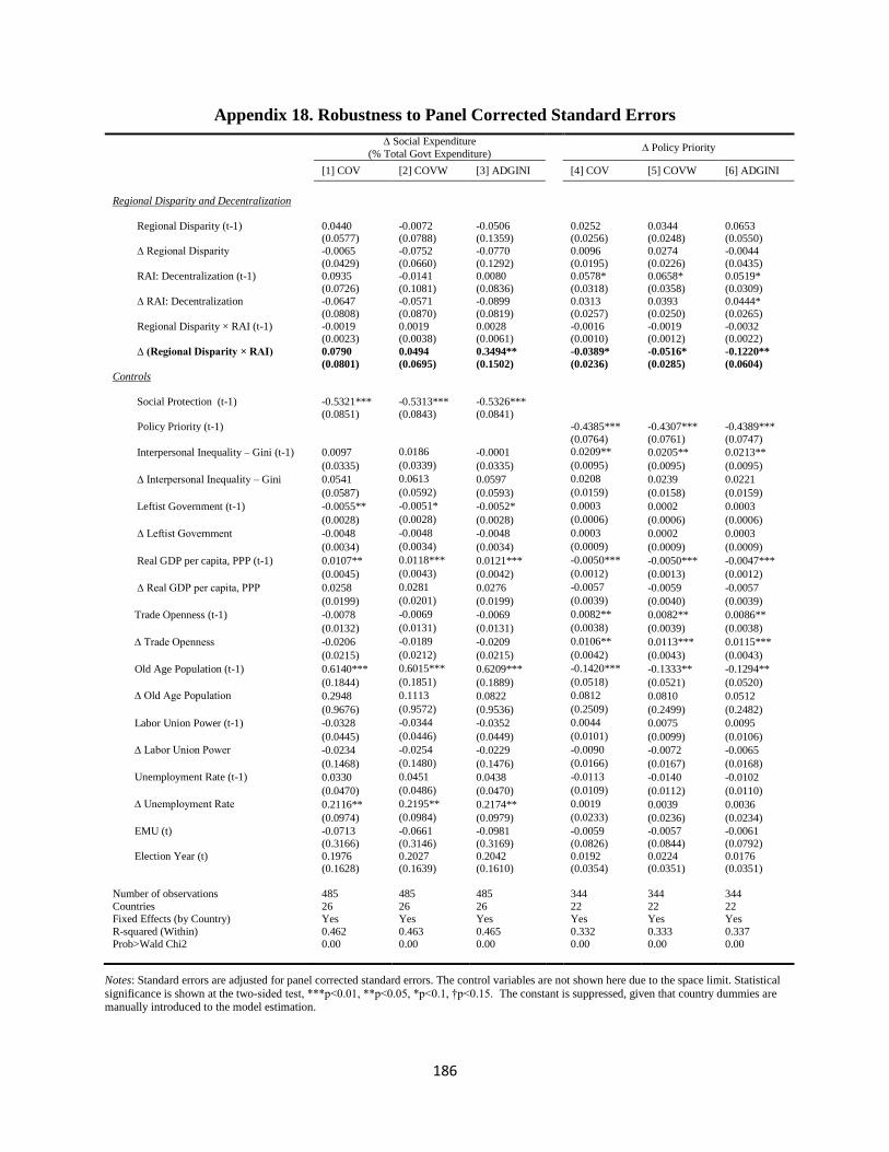
186
Appendix 18. Robustness to Panel Corrected Standard Errors
∆ Social Expenditure
(% Total Govt Expenditure) ∆ Policy Priority
[1] COV [2] COVW [3] ADGINI [4] COV [5] COVW [6] ADGINI
Regional Disparity and Decentralization
Regional Disparity (t-1) 0.0440 -0.0072 -0.0506 0.0252 0.0344 0.0653 (0.0577) (0.0788) (0.1359) (0.0256) (0.0248) (0.0550)
∆ Regional Disparity -0.0065 -0.0752 -0.0770 0.0096 0.0274 -0.0044
(0.0429) (0.0660) (0.1292) (0.0195) (0.0226) (0.0435)
RAI: Decentralization (t-1) 0.0935 -0.0141 0.0080 0.0578* 0.0658* 0.0519*
(0.0726) (0.1081) (0.0836) (0.0318) (0.0358) (0.0309)
∆ RAI: Decentralization -0.0647 -0.0571 -0.0899 0.0313 0.0393 0.0444*
(0.0808) (0.0870) (0.0819) (0.0257) (0.0250) (0.0265)
Regional Disparity × RAI (t-1) -0.0019 0.0019 0.0028 -0.0016 -0.0019 -0.0032 (0.0023) (0.0038) (0.0061) (0.0010) (0.0012) (0.0022)
∆ (Regional Disparity × RAI) 0.0790 0.0494 0.3494** -0.0389* -0.0516* -0.1220**
(0.0801) (0.0695) (0.1502) (0.0236) (0.0285) (0.0604)
Controls
Social Protection (t-1) -0.5321*** -0.5313*** -0.5326***
(0.0851) (0.0843) (0.0841) Policy Priority (t-1) -0.4385*** -0.4307*** -0.4389***
(0.0764) (0.0761) (0.0747)
Interpersonal Inequality – Gini (t-1) 0.0097 0.0186 -0.0001 0.0209** 0.0205** 0.0213**
(0.0335) (0.0339) (0.0335) (0.0095) (0.0095) (0.0095)
∆ Interpersonal Inequality – Gini 0.0541 0.0613 0.0597 0.0208 0.0239 0.0221
(0.0587) (0.0592) (0.0593) (0.0159) (0.0158) (0.0159)
Leftist Government (t-1) -0.0055** -0.0051* -0.0052* 0.0003 0.0002 0.0003
(0.0028) (0.0028) (0.0028) (0.0006) (0.0006) (0.0006)
∆ Leftist Government -0.0048 -0.0048 -0.0048 0.0003 0.0002 0.0003
(0.0034) (0.0034) (0.0034) (0.0009) (0.0009) (0.0009)
Real GDP per capita, PPP (t-1) 0.0107** 0.0118*** 0.0121*** -0.0050*** -0.0050*** -0.0047***
(0.0045) (0.0043) (0.0042) (0.0012) (0.0013) (0.0012)
∆ Real GDP per capita, PPP 0.0258 0.0281 0.0276 -0.0057 -0.0059 -0.0057
(0.0199) (0.0201) (0.0199) (0.0039) (0.0040) (0.0039)
Trade Openness (t-1) -0.0078 -0.0069 -0.0069 0.0082** 0.0082** 0.0086**
(0.0132) (0.0131) (0.0131) (0.0038) (0.0039) (0.0038)
∆ Trade Openness -0.0206 -0.0189 -0.0209 0.0106** 0.0113*** 0.0115***
(0.0215) (0.0212) (0.0215) (0.0042) (0.0043) (0.0043)
Old Age Population (t-1) 0.6140*** 0.6015*** 0.6209*** -0.1420*** -0.1333** -0.1294**
(0.1844) (0.1851) (0.1889) (0.0518) (0.0521) (0.0520)
∆ Old Age Population 0.2948 0.1113 0.0822 0.0812 0.0810 0.0512
(0.9676) (0.9572) (0.9536) (0.2509) (0.2499) (0.2482)
Labor Union Power (t-1) -0.0328 -0.0344 -0.0352 0.0044 0.0075 0.0095
(0.0445) (0.0446) (0.0449) (0.0101) (0.0099) (0.0106)
∆ Labor Union Power -0.0234 -0.0254 -0.0229 -0.0090 -0.0072 -0.0065
(0.1468) (0.1480) (0.1476) (0.0166) (0.0167) (0.0168)
Unemployment Rate (t-1) 0.0330 0.0451 0.0438 -0.0113 -0.0140 -0.0102
(0.0470) (0.0486) (0.0470) (0.0109) (0.0112) (0.0110)
∆ Unemployment Rate 0.2116** 0.2195** 0.2174** 0.0019 0.0039 0.0036
(0.0974) (0.0984) (0.0979) (0.0233) (0.0236) (0.0234)
EMU (t) -0.0713 -0.0661 -0.0981 -0.0059 -0.0057 -0.0061
(0.3166) (0.3146) (0.3169) (0.0826) (0.0844) (0.0792)
Election Year (t) 0.1976 0.2027 0.2042 0.0192 0.0224 0.0176 (0.1628) (0.1639) (0.1610) (0.0354) (0.0351) (0.0351)
Number of observations 485 485 485 344 344 344
Countries 26 26 26 22 22 22
Fixed Effects (by Country) Yes Yes Yes Yes Yes Yes
R-squared (Within) 0.462 0.463 0.465 0.332 0.333 0.337
Prob>Wald Chi2 0.00 0.00 0.00 0.00 0.00 0.00
Notes: Standard errors are adjusted for panel corrected standard errors. The control variables are not shown here due to the space limit. Statistical
significance is shown at the two-sided test, ***p<0.01, **p<0.05, *p<0.1, †p<0.15. The constant is suppressed, given that country dummies are manually introduced to the model estimation.
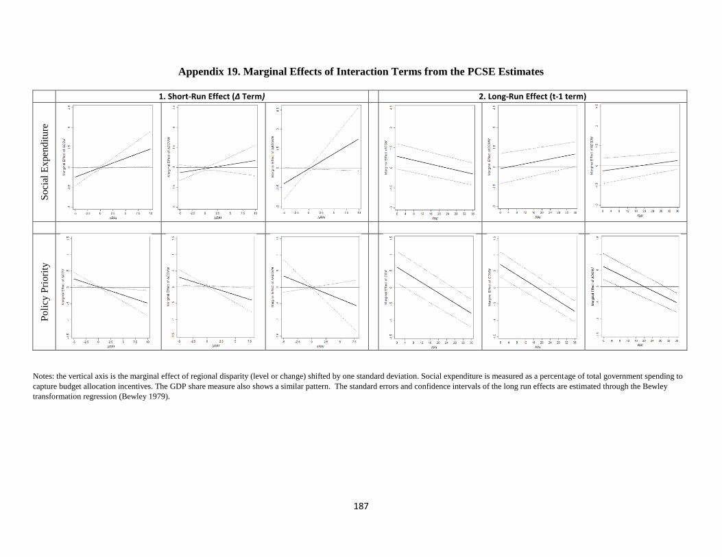
187
Appendix 19. Marginal Effects of Interaction Terms from the PCSE Estimates
1. Short-Run Effect (∆ Term) 2. Long-Run Effect (t-1 term)
Soci
al E
xpen
dit
ure
Poli
cy P
riori
ty
Notes: the vertical axis is the marginal effect of regional disparity (level or change) shifted by one standard deviation. Social expenditure is measured as a percentage of total government spending to
capture budget allocation incentives. The GDP share measure also shows a similar pattern. The standard errors and confidence intervals of the long run effects are estimated through the Bewley
transformation regression (Bewley 1979).

188
Appendix 20. Robustness to Panel Jackknife Analysis of Interaction Effects
(a) ∆ Social Expenditure (% GDP) (b) ∆ Policy Priority
Notes: The panel Jackknife estimates are presented on the full models from Table 13 and Table 14. Each country enlisted on the vertical axis represents 25 countries that
omit this country from the analysis iteratively with replacement. Confidence intervals are reported at the 90%. For the policy priority, the analysis is conducted across 21
countries due to the data availability from 1990 to 2010.

189
Appendix 21: Descriptive Statistics for Additional Variables
Variables Descriptions Mean Std.Dev. Min Max Sources
Alternative Dependent Variables
Social Expenditure Social expenditure (% Total general government expenditure). See
detail categories same as the above indicated in Appendix 12.
47.89 7.01 11.07 76.01 The OECD Social
Expenditure Database
(SOCX)
Social Security Transfer Social security transfer (% of GDP) accounts for social assistance
grants and welfare benefits paid by the general government (e.g.,
benefit for sickness, old-age, family allowances, etc.).
13.82 3.35 6.17 23.40 Comparative Political
Dataset; OECD
National Account
Statistics
Health Expenditure Current expenditure on healthcare (% of GDP). Provided by the
general government.
5.66 1.19 2.41 9.08 OECD Health
Expenditure and
Financing
Social Protection Social protection expenditure by the central government (% of GDP)
on sickness and disability, old-age, survivors, family children,
unemployment, housing, R& D, social exclusion, etc.
16.98 4.17 8.31 25.58 Government Finance
Statistics Online
Database.
Social protection expenditure by the general government (% of GDP) 14.04 3.66 5.17 22.56
Alternative Independent Variables
Self-rule This is an index measure to score the authority exercised by a
regional government over the people living within its territory.
Country scores are aggregated measures from each regional their and
individual regional government in that country. They account for a
regional government’s institutional autonomy (1-4), authoritative
competence in policy making (0-4), ability to control over local
taxation (0-4), borrowing without centrally imposing restrictions (0-
3), and having an independent legislature or executive (0-4).
Empirical ranges may go beyond the dimensional sum (18) due to
additive values by the multiple existences of regional tiers within a
country.
12.52 6.98 6.10 29.95 Regional Authority
Index (RAI)
Database; Hoogle et al
(2015).
Shared-rule The shared rule also a variable to capture the degree of the authority
exercised by a regional government particularly in the country as a
whole. Scores are the sum of policy indices across five dimensions:
Law making (0-2), executive control (0-2), fiscal control (0-2),
borrowing control (0-2), and constitutional reform (0-4).
3.37 4.39 0 15.01