Macroeconomic Challenges Facing

Low-Income Countries

New Perspectives

January 30–31, 2014

Income Inequality, Trade and Financial

Openness

G. C. Lim

University of Melbourne

Paul D. McNelis

Fordham University

Paper presented at the joint RES-SPR Conference on “Macroeconomic Challenges Facing

Low-Income Countries”

Hosted by the International Monetary Fund

With support from the UK Department of International Development (DFID)

Washington, DC—January 30–31, 2014

The views expressed in this paper are those of the author(s) only, and the presence of

them, or of links to them, on the IMF website does not imply that the IMF, its Executive

Board, or its management endorses or shares the views expressed in the paper.

Income Inequality, Trade and Financial

Openness

G.C. Lim and Paul D. McNelis

January 2014

Abstract

This paper examines the relationships of the Gini coefficient with

trade-openness, aid and foreign direct investment flows. Panel data es-

timates are provided for the overall data set (42 low to middle income

countries). We find empirically, that trade openness is more effective

than either foreign direct investent or foreign aid for changing income in-

equality, but its effectiveness depends on the stage of development. We

then develop a model of a small economy with varying degrees of open-

ness. We find that countries with high labour intensity in production, and

greater openness generate lower inequality in response to favorable shocks

to export demand and terms of trade. Both our empirical and simulation

results suggest that trade and financial openness can be effective policies

for reducing inequality in low income countries, provided that the gains

from capital are re-distributed.

Keywords:

JEL classification:

Lim: g.lim@unimelb.edu.au; Melbourne Institute of Economic and So-

cial Research, University of Melbourne, Parkville, Australia.

McNelis: mcnelis@fordham.edu; Department of Finance, Graduate

School of Business Administration, Fordham University, New York 10019.

McNelis’s research for this project took place while he was a visiting

scholar at the Department of Economic Studies at the Bank of Portu-

gal.

This paper is part of an IMF research project on macroeconomic pol-

icy in low-income countries supported by the UK Department for Interna-

tional Development (DFID). The views expressed in this paper are those

of the authors and do not necessarily reflect those of the DFID, IMF or

the Bank of Portugal.

1

1 Introduction

It has been more than forty years since Hirschman and Rothschild (1973) drew

attention to the changing tolerance for inequality in the process of economic

development. Citing the civil wars in Pakistan and Nigeria taking place in that

period, these authors argued that the "tunnel effect" — the willingness of certain

segments of the population to remain behind, accepting relative deprivation

while others get ahead, in the hope that the advancement would later become

more widespread — may be short lived. These authors challenged the prevailing

conventional wisdom of Kuznets (1955) and Kaldor (1957).

Kuznets formulated the relationship between economic growth and inequal-

ity as an inverted-U curve. In the early stages of development, as an economy

moved from an informal rural structure to an industrialized one, there would

be a transition process of greater inequality as the industrial sector grew at

the expense of the agrarian rural sector. As Turnovsky (2013) observes, the

Kuznets explanation of an inverted-U curve rests on "dual economy" dynamics.

Kaldor’s reasoning was more direct. The rich save more of their income

than the poor, so that redistribution in favor of the rich would lead to greater

savings and thus resources for investment and growth.

Kuznets and Kaldor offer different views of the inequality-growth relation.

In the Kuznets view, inequality increases as a result of the initial stages of

growth while in the Kaldor scenario, inequality is needed to generate growth.

As Deaton (2013) notes, inequality is part and parcel of development. As some

members of the population become successful in making the "Great Escape"

from poverty and deprivation, others may be left behind. A key question is

what policies enhance the changes of succeeding generations to make a similar

great escape?

In the years, since the Hirschman-Rothschild challenge, and the conventional

wisdom handed down by Kuznets and Kaldor, there has been progress in our

understanding of the relationship between growth and inequality. The belief

that economic growth generally alleviates poverty and reduces income inequality

is now widely-held and supported empirically by many studies. Dollar and Kray

(2002), for example, show in their highly cited article entitled “Growth is Good

for the Poor,” that economic growth and poverty reduction are related on a

one-to-one basis. In a later paper, Dollar and Kray (2004) argue that increased

trade leads to economic growth as well as poverty reduction in poor countries.

Few, if any, can dispute that fact that the advances in economic growth in many

parts of the world, particularly in East and South Asia, have brought hundreds

of millions out of poverty.

The last forty years have also witnessed the growth and spread of new tech-

nology as well as trade and financial liberalization across the world. Both of

these are seen as conduits of growth but their implications for income distrib-

ution are less clear-cut. A recent study by Jaumotte, Lall and Papageorgiou

(2008) suggested that while technological change has been a significant driver

of the rise in inequality across both developed and developing countries, the

contribution of globalization has been relatively minor. This is because trade

2

liberalization generally results in a reduction in income inequality while finan-

cial liberalization generally results in an increase in income inequality. Thus the

effects of globalization in trade and finance on income inequality tend to offset

each other.

The finding that the effect of globalization on inequality is minor has signif-

icant implications. Does it mean that designing policies to promote education,

skills and technological progress are the only viable options to promote growth

and equality? Is openness no longer an effective avenue for a low income coun-

try, with rich natural resources, but with a largely low-skilled labour force, to

achieve growth and equality? Which mechanisms ensure that growth (via trade

and/or financial liberalization) are or are not conducive to promoting income

equality?

This first part of the paper examines empirically the relationship between

income inequality, economic growth, and openness based on an annual data set

of 42 countries (with GDP per capital close to or below the world’s GDP per

capita) for the period 1992-2007. Is economic growth more likely to reduce

income inequality in countries which are relatively more open?

Openness is usually measured as the ratio of trade (sum of exports and

imports) to GDP. We also examine openness in terms of the ratio of foreign

direct investment as well as foreign aid relative to GDP.

The data are also decomposed into three subsets - low income countries

(which includes almost all countries eligible for Poverty Reduction and Growth

Trust support in International Monetary Fund lending programs), lower-middle

income countries (corresponding to classification suggested by the World Bank)

and upper-middle (comprising countries usually classified as Emerging Mar-

kets). Breaking the panel set into three groups allowed us to analyse the effect

of growth and relative income on inequality, conditioned on the stage of develop-

ment. Furthermore, apriori, countries designated as PRGT-eligible are excepted

to be more receptive to foreign aid inflows, while those countries designated as

EM are expected to be more receptive to foreign direct investment.

The panel results with fixed country and time effects show a significant nega-

tive association between the Gini and growth, as well as significant relationships

between the Gini and trade and financial openness. However both the intensity

and the direction of effect varied across the three subsets mainly because the

panel results masked a myriad of possibilities. For example, a closer look at the

correlations between the Gini and openness (both trade and financial) showed

that they varied from close to -1 to close to +1.

In order to understand better the relationships between openness (trade

and financial) and income inequality (as measured by the Gini coefficient), the

second part of this paper develops, calibrates and simulates a model of a small

open economy. Our specification captures key features noted by the IMF,

namely that the countries in our dataset tend to be heavily dependent on exports

of natural resources; they are less diversified and vulnerable to terms of trade

shocks (especially of food and oil); their financial system is centered around

banks and the exchange rate is usually fixed or pegged.

We simulate the model for shocks to the export sector (in the form of export

3

demand and terms of trade changes), for varying degrees of openness. We also

explore the importance of labour intensity in the production of traded and non-

traded goods for understanding the mechanisms that affect income inequality.

The paper is organized as follows. Section 2 of the paper is devoted to the

empirical analysis while section 3 sets out the model. In section 4, the stylized

model is simulated to yield insights about the empirical results. Concluding

remarks are in section 5.

2 Empirical Analysis

2.1 Data

The panel data set consists of annual data from 1992-2007 for 42 countries, all

with GDP per capital close to or below the world’s GDP per capita. The vari-

ables are: the Gini coefficients on inequality1, GDP growth rates (), relative

per-capita GDP (, that is the country’s per-capita GDP relative to the world

per capita GDP), government spending to GDP ratio (), openness in trade

(). The data set also includes the foreign aid to GDP ratio () and the

foreign direct investment to GDP ratio (), variables that represent financial

openness in terms of receptivity to capital-account inflows.2

Table 1 gives the sample means (in percentage terms) for each country in the

data set between 1992 and 2007. Since the data set spans a range of economies

with very different characteristics, we also ranked them according to their av-

erage GDP per capita and divided them into three classes - low income, lower-

middle and upper-middle income using the World Bank classification as a guide.

Twelve of the PRGT countries are in the low-income group (with GDP per

capita under 35 per cent of the world GDP per capita), the other five are clas-

sified as lower-middle income countries. The 10 upper-middle income countries

have GDP per capital around the world’s average GDP per capita.

Table 1 shows great variation among the indicators. In terms of GDP per

capita relative to the world’s GDP per capita, the poorest country is Tanzania

with a sample mean of 10.5 per cent. All PRGT countries plus Pakistan have

sample averages under 50 per cent. Countries with per-capita income close to

the world’s per capita GDP are the emerging countries which includes the South

American countries of Costa Rica, Venezuela and Brazil, the African countries

which include Tunisia and South Africa and the Asian country of Thailand.

1While we are only concerned with income inequality, we recognise that there are other

measures of inequality. For example, regional inequality is important, especially for very large

economies such as India and Brazil. Daumal (2010) found with time-series estimation that

Brazil’s trade openness contributed to a reduction in regional inequality while the opposite

was true for India.2The data, with the exception of the foreign aid and foreign direct investment ratios

are described in Solt (2009) and Claessens and van Horen (2012) and used in recent papers

by Delis, Hasan, and Myonidis (2013) and Delis, Hasan, and Kazakis (2013) to examine,

respectively, the relationship between foreign bank ownership with income inequality, and

banking-sector de-regulations with inequality.

4

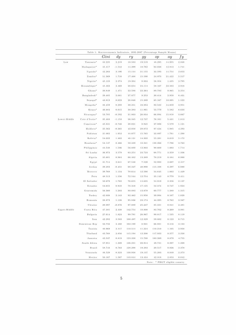
Tab le 1 : M a c ro e c o n om ic In d i c a t o r s , 1 9 9 2 -2 0 0 7 (P e r c e n t a g e S am p le M e a n s )

L ow Ta n z a n ia * 3 4 .2 2 5 2 .2 1 9 1 0 .5 8 3 1 9 .5 1 9 4 8 .2 9 5 1 4 .9 5 5 2 .8 3 8

M a d a g a s c a r * 4 5 .4 1 7 -1 .5 4 2 1 4 .3 9 9 1 0 .7 6 2 6 2 .0 2 6 1 2 .8 1 3 1 .7 4 1

U g a n d a * 4 2 .2 0 3 3 .1 9 6 1 5 .1 4 4 3 1 .1 5 5 3 2 .5 9 3 1 4 .7 5 4 3 .0 5 3

Z am b ia * 5 1 .3 6 9 1 .7 1 6 1 7 .4 6 8 1 5 .5 9 0 2 4 .0 7 3 2 1 .4 2 2 5 .5 1 7

N ig e r ia * 4 5 .1 2 3 3 .2 7 4 1 9 .3 8 4 8 .8 0 4 5 6 .3 5 4 1 .4 3 5 3 .7 9 5

M o z am b iq u e * 4 5 .4 0 3 3 .4 6 9 2 0 .6 5 4 2 4 .1 1 4 5 8 .1 6 7 3 3 .4 8 3 3 .9 1 8

G h a n a * 3 9 .8 4 9 1 .4 7 1 2 2 .5 8 0 2 3 .3 6 4 8 9 .7 8 3 9 .9 6 5 2 .2 5 4

B a n g la d e s h * 2 9 .4 8 5 2 .0 8 1 2 7 .8 7 7 9 .2 5 3 3 0 .4 1 4 2 .9 5 9 0 .4 3 1

S e n e g a l* 4 3 .8 1 3 0 .0 2 3 2 8 .0 4 0 1 5 .3 8 9 6 5 .1 6 7 1 0 .0 9 5 1 .5 2 2

M o n g o l i a * 3 2 .4 5 9 0 .2 8 8 3 0 .2 5 1 1 6 .8 8 4 9 2 .5 2 2 1 4 .6 5 9 3 .9 5 1

K enya * 4 6 .6 8 4 0 .0 1 5 3 0 .3 8 3 1 1 .9 6 1 5 3 .7 7 9 5 .5 8 2 0 .6 3 3

N ic a r a g u a * 5 3 .7 8 5 -0 .5 9 2 3 1 .8 6 3 2 6 .0 3 4 6 6 .8 9 4 1 5 .8 1 8 3 .6 6 7

L ow e r -M id d le C o t e d ’ Iv o i r e * 3 5 .4 0 3 -1 .1 5 3 3 6 .3 4 5 1 2 .7 3 7 7 6 .1 6 1 5 .4 3 1 1 .8 1 3

C am e ro o n * 4 5 .8 3 1 -0 .7 4 6 3 8 .0 2 1 8 .9 4 5 3 7 .0 8 6 5 .5 7 9 1 .1 2 1

M o ld ova * 3 5 .5 6 2 -0 .3 6 5 4 3 .0 5 0 2 9 .0 7 3 8 7 .4 2 4 5 .0 8 5 4 .2 9 3

P a k is t a n 3 1 .0 0 2 1 .9 5 3 4 4 .0 7 7 1 5 .7 6 5 3 3 .8 9 7 1 .7 9 1 1 .2 9 8

B o l iv ia * 5 4 .0 2 2 1 .4 0 3 4 8 .1 3 1 1 4 .2 0 2 5 5 .3 9 1 8 .6 1 9 5 .1 7 2

H o n d u ra s * 5 4 .1 4 7 0 .4 6 6 5 0 .4 3 9 1 8 .2 4 1 1 2 0 .2 6 6 7 .7 9 6 3 .7 6 3

P h i l ip p in e s 4 4 .5 4 8 1 .5 9 6 5 6 .8 8 9 1 2 .9 0 3 9 9 .6 0 9 1 .0 8 3 1 .7 1 4

S r i L a n ka 3 6 .9 7 3 3 .5 7 9 6 3 .2 5 4 2 3 .7 2 3 6 8 .7 7 1 3 .3 5 9 1 .3 3 6

A lg e r ia 3 5 .6 8 1 0 .9 6 4 6 6 .4 0 2 1 3 .3 8 9 7 0 .2 1 9 0 .4 8 4 0 .9 0 0

E g y p t 3 1 .7 1 4 2 .6 4 1 6 7 .5 4 0 7 .5 2 0 5 2 .9 9 3 2 .6 8 7 2 .4 1 7

J o rd a n 3 9 .2 8 3 -0 .4 5 5 6 8 .3 4 7 4 0 .9 9 0 1 1 5 .1 0 8 6 .2 9 7 6 .0 0 0

M o ro c c o 3 9 .7 6 8 1 .1 3 4 7 0 .6 1 4 1 2 .5 6 6 5 4 .6 4 5 1 .6 6 3 1 .4 4 9

P e ru 4 8 .5 1 3 1 .5 5 6 7 2 .5 4 4 1 2 .7 5 4 3 5 .1 4 3 0 .7 7 9 3 .4 1 1

E l S a lva d o r 5 0 .6 7 9 1 .7 6 2 7 6 .6 5 5 1 4 .6 3 5 5 4 .0 1 9 2 .3 5 6 2 .1 3 7

E cu a d o r 5 4 .6 5 5 0 .9 1 0 7 8 .3 1 0 1 7 .1 2 5 5 2 .4 7 4 0 .7 4 7 1 .9 2 4

G u a t em a la 5 6 .3 0 0 1 .2 0 3 8 0 .8 8 3 1 3 .0 7 9 6 0 .7 7 7 1 .3 8 0 1 .3 1 5

Tu rk e y 4 2 .0 3 8 2 .1 4 3 9 2 .4 6 2 1 5 .9 5 0 3 9 .9 9 4 0 .1 0 7 1 .0 2 9

R om a n ia 2 8 .8 7 3 1 .1 2 6 9 5 .8 3 6 2 3 .1 7 4 4 4 .3 9 5 0 .7 6 2 3 .5 6 7

U k ra in e 2 9 .0 9 7 -0 .8 7 6 9 7 .8 8 9 2 5 .2 4 7 8 5 .3 3 1 0 .8 4 1 2 .4 8 1

U p p e r -M id d le C o s t a R ic a 4 7 .4 8 1 2 .4 3 8 1 4 2 .7 5 4 1 8 .8 0 0 8 3 .7 6 2 0 .2 6 9 3 .8 0 1

B u lg a r ia 2 7 .6 1 4 1 .8 2 4 9 9 .7 9 1 2 6 .9 6 7 9 9 .8 1 7 1 .5 3 5 8 .1 1 9

I r a n 4 2 .2 9 2 3 .5 0 3 1 0 0 .4 9 7 1 2 .3 2 9 5 9 .8 0 2 0 .1 2 3 0 .7 1 5

D om in i c a n R ep 5 0 .7 5 6 3 .4 8 0 1 0 2 .1 9 9 8 .9 3 1 6 6 .8 8 1 0 .4 1 6 3 .1 8 3

Tu n is ia 4 0 .9 6 9 3 .4 1 7 1 1 0 .5 1 4 1 1 .3 2 4 1 1 0 .2 1 0 1 .1 0 5 2 .9 5 0

T h a i l a n d 4 3 .7 6 8 3 .8 5 6 1 1 5 .1 9 4 1 2 .2 0 0 1 1 7 .9 2 3 0 .2 7 7 3 .2 3 0

J am a ic a 4 2 .5 3 7 0 .8 1 9 1 2 3 .3 2 0 1 5 .7 0 8 1 0 3 .2 6 9 0 .8 7 9 4 .7 5 5

S o u th A fr i c a 5 7 .9 5 1 1 .3 0 9 1 2 6 .2 2 1 2 0 .9 1 4 4 9 .7 2 1 0 .2 9 7 1 .2 0 9

B ra z i l 5 8 .7 4 3 0 .7 6 3 1 2 8 .2 9 0 1 9 .3 8 3 2 0 .5 1 7 0 .0 2 6 2 .3 7 8

Ve n e z u e la 4 6 .5 2 9 0 .3 2 3 1 3 0 .9 3 8 1 9 .1 3 7 5 5 .2 0 3 0 .0 4 9 2 .3 7 3

M ex ic o 5 0 .1 0 7 1 .5 6 7 1 4 3 .8 4 4 1 3 .4 3 4 4 2 .3 1 8 2 .8 5 3 0 .0 4 2

N o t e : * P RG T e l ig ib le c o u n t r y

5

The highest mean Gini coefficient is for Brazil and the lowest is for Bulgaria.

For economic growth, the top three performers are Thailand, Sri Lanka and Iran,

while Jordan has the highest sample mean value for the Government spending

to GDP ratio. The Index of trade openness spans the range from 20.5 (Brazil)

to 120.3 (Honduras). Some countries received virtually no foreign investment,

such as Bangladesh, while the foreign aid flow for Mozambique is more than a

third of its GDP.

Table 2 summarizes the descriptive statistics of these indicators for the full

sample of 42 countries as well as the three income groups. The data show that

the Gini coefficients and the ratio of government spending to GDP are similar

across the samples. Openness and the ratio of foreign direct investment to GDP

is also surprisingly similar across the subsets. However, the Aid/GDP ratio is

much higher for the Low-income (PRGT) countries.

Table 2: Statistical Properties of Indices (Percentage)

Full sample (42)

mean 43.323 1.375 67.616 17.237 65.076 5.234 2.763

median 43.390 1.423 66.178 14.923 59.253 1.652 2.055

minimum 23.430 -17.900 9.484 5.892 13.310 -0.661 -2.499

maximum 61.780 15.572 166.476 52.362 144.492 74.137 32.947

Low-Income Countries (12)

mean 42.485 1.301 22.386 17.736 56.672 13.162 2.777

median 42.930 0.957 22.378 15.921 55.475 11.137 2.210

minimum 26.210 -9.350 9.484 5.892 17.406 0.367 -0.014

maximum 60.460 15.572 38.479 35.698 133.348 74.137 11.471

Lower-Middle Income Countries (20)

mean 41.431 1.033 67.374 17.949 67.176 2.919 2.763

median 41.060 1.330 67.766 14.764 61.556 1.593 1.710

minimum 23.430 -17.900 27.718 7.302 23.858 0.000 -2.499

maximum 61.780 9.158 129.971 52.362 141.148 19.163 32.947

Upper-Middle Income Countries (10)

mean 48.113 2.147 122.377 15.216 70.960 0.350 2.747

median 47.438 2.121 124.808 14.335 64.024 0.163 2.645

minimum 35.670 -4.434 80.573 7.992 13.310 -0.661 -0.070

maximum 60.480 9.112 166.476 22.906 144.492 3.345 9.425

As Deaton (2013) points out, sample means may mask important changes

talking place over time. To better understand the relationships between the

Gini coefficient and per-capita income and openness, we plot scatter diagrams

relating the Gini to these two variables at the beginning of the sample and at

the end of the sample, 1992 and 2007, respectively.

Figure 1 shows that both the per-capita income and the degree of openness

have increased markedly from the beginning to the end of the period. The x-

symbols represent the scatter diagram for 1992 and the o-symbols, the scatter for

6

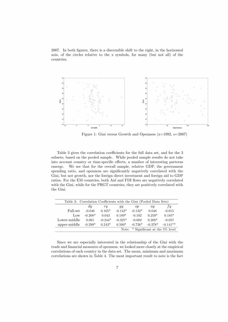
2007. In both figures, there is a discernible shift to the right, in the horizontal

axis, of the circles relative to the x symbols, for many (but not all) of the

countries.

-10 -5 0 5 10 1520

25

30

35

40

45

50

55

60

65

Growth

Gin

i

0 50 100 15020

25

30

35

40

45

50

55

60

65

Openness

Gin

i

Figure 1: Gini versus Growth and Openness (x=1992, o=2007)

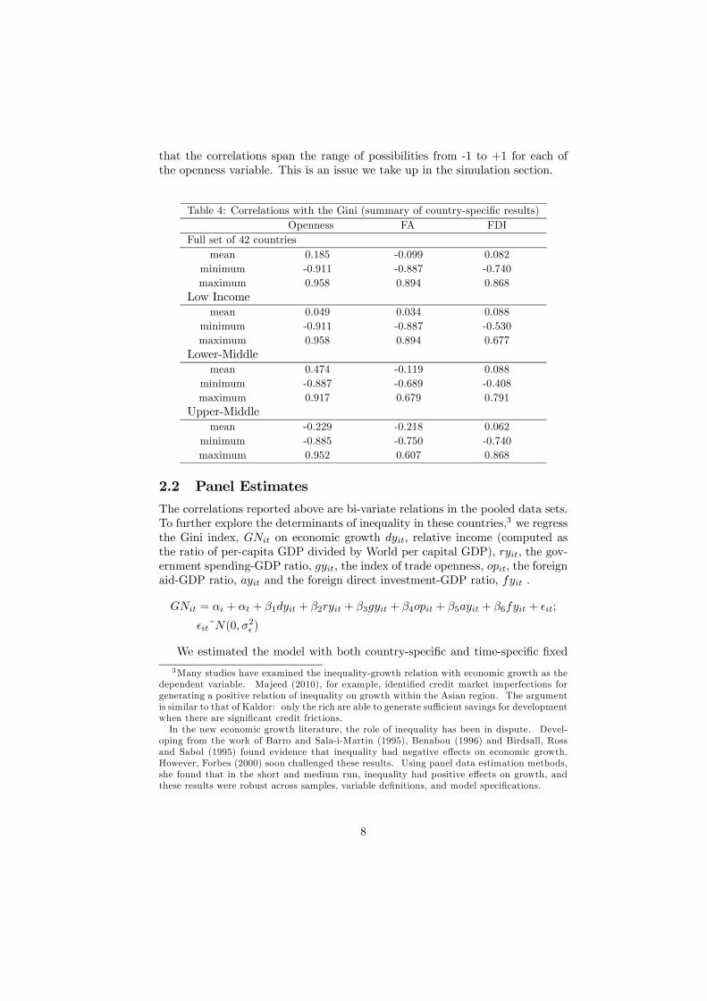
Table 3 gives the correlation coefficients for the full data set, and for the 3

subsets, based on the pooled sample. While pooled sample results do not take

into account country or time-specific effects, a number of interesting patterns

emerge. We see that for the overall sample, relative GDP, the government

spending ratio, and openness are significantly negatively correlated with the

Gini, but not growth, nor the foreign direct investment and foreign aid to GDP

ratios. For the EM countries, both Aid and FDI flows are negatively correlated

with the Gini, while for the PRGT countries, they are positively correlated with

the Gini.

Table 3: Correlation Coefficients with the Gini (Pooled Data Sets)

Full-set -0.048 0.165* -0.142* -0.132* 0.048 -0.015

Low -0.208* 0.043 0.189* -0.102 0.259* 0.185*

Lower-middle 0.001 -0.244* -0.325* -0.002 0.208* -0.057

upper-middle -0.299* 0.243* 0.500* -0.726* -0.378* -0.141**

Note: * Significant at the 5% level

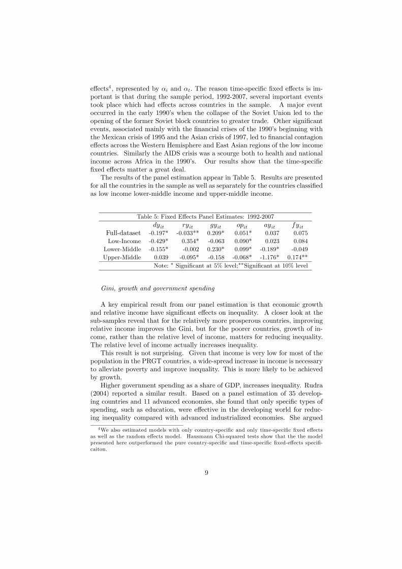
Since we are especially interested in the relationship of the Gini with the

trade and financial measures of openness, we looked more closely at the empirical

correlations of each country in the data set. The mean, minimum and maximum

correlations are shown in Table 4. The most important result to note is the fact

7

that the correlations span the range of possibilities from -1 to +1 for each of

the openness variable. This is an issue we take up in the simulation section.

Table 4: Correlations with the Gini (summary of country-specific results)

Openness FA FDI

Full set of 42 countries

mean 0.185 -0.099 0.082

minimum -0.911 -0.887 -0.740

maximum 0.958 0.894 0.868

Low Income

mean 0.049 0.034 0.088

minimum -0.911 -0.887 -0.530

maximum 0.958 0.894 0.677

Lower-Middle

mean 0.474 -0.119 0.088

minimum -0.887 -0.689 -0.408

maximum 0.917 0.679 0.791

Upper-Middle

mean -0.229 -0.218 0.062

minimum -0.885 -0.750 -0.740

maximum 0.952 0.607 0.868

2.2 Panel Estimates

The correlations reported above are bi-variate relations in the pooled data sets.

To further explore the determinants of inequality in these countries,3 we regress

the Gini index, on economic growth relative income (computed as

the ratio of per-capita GDP divided by World per capital GDP), the gov-

ernment spending-GDP ratio, , the index of trade openness, the foreign

aid-GDP ratio, and the foreign direct investment-GDP ratio, .

= + + 1 + 2 + 3 + 4 + 5 + 6 + ;

˜(0 2 )

We estimated the model with both country-specific and time-specific fixed

3Many studies have examined the inequality-growth relation with economic growth as the

dependent variable. Majeed (2010), for example, identified credit market imperfections for

generating a positive relation of inequality on growth within the Asian region. The argument

is similar to that of Kaldor: only the rich are able to generate sufficient savings for development

when there are significant credit frictions.

In the new economic growth literature, the role of inequality has been in dispute. Devel-

oping from the work of Barro and Sala-i-Martin (1995), Benabou (1996) and Birdsall, Ross

and Sabol (1995) found evidence that inequality had negative effects on economic growth.

However, Forbes (2000) soon challenged these results. Using panel data estimation methods,

she found that in the short and medium run, inequality had positive effects on growth, and

these results were robust across samples, variable definitions, and model specifications.

8

effects4, represented by and The reason time-specific fixed effects is im-

portant is that during the sample period, 1992-2007, several important events

took place which had effects across countries in the sample. A major event

occurred in the early 1990’s when the collapse of the Soviet Union led to the

opening of the former Soviet block countries to greater trade. Other significant

events, associated mainly with the financial crises of the 1990’s beginning with

the Mexican crisis of 1995 and the Asian crisis of 1997, led to financial contagion

effects across the Western Hemisphere and East Asian regions of the low income

countries. Similarly the AIDS crisis was a scourge both to health and national

income across Africa in the 1990’s. Our results show that the time-specific

fixed effects matter a great deal.

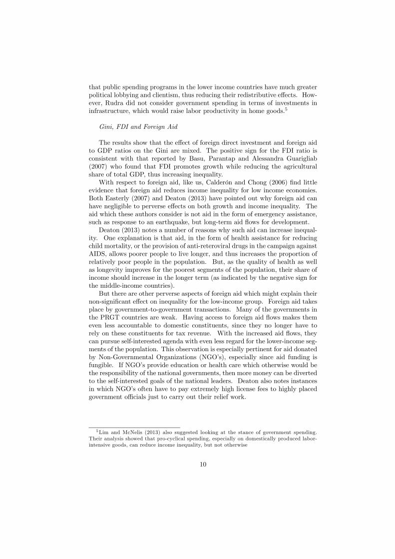
The results of the panel estimation appear in Table 5. Results are presented

for all the countries in the sample as well as separately for the countries classified

as low income lower-middle income and upper-middle income.

Table 5: Fixed Effects Panel Estimates: 1992-2007

Full-dataset -0.197* -0.033** 0.209* 0.051* 0.037 0.075

Low-Income -0.429* 0.354* -0.063 0.090* 0.023 0.084

Lower-Middle -0.155* -0.002 0.230* 0.099* -0.189* -0.049

Upper-Middle 0.039 -0.095* -0.158 -0.068* -1.176* 0.174**

Note: ∗ Significant at 5% level;∗∗Significant at 10% level

Gini, growth and government spending

A key empirical result from our panel estimation is that economic growth

and relative income have significant effects on inequality. A closer look at the

sub-samples reveal that for the relatively more prosperous countries, improving

relative income improves the Gini, but for the poorer countries, growth of in-

come, rather than the relative level of income, matters for reducing inequality.

The relative level of income actually increases inequality.

This result is not surprising. Given that income is very low for most of the

population in the PRGT countries, a wide-spread increase in income is necessary

to alleviate poverty and improve inequality. This is more likely to be achieved

by growth.

Higher government spending as a share of GDP, increases inequality. Rudra

(2004) reported a similar result. Based on a panel estimation of 35 develop-

ing countries and 11 advanced economies, she found that only specific types of

spending, such as education, were effective in the developing world for reduc-

ing inequality compared with advanced industrialized economies. She argued

4We also estimated models with only country-specific and only time-specific fixed effects

as well as the random effects model. Hausmann Chi-squared tests show that the the model

presented here outperformed the pure country-specific and time-specific fixed-effects specifi-

caiton.

9

that public spending programs in the lower income countries have much greater

political lobbying and clientism, thus reducing their redistributive effects. How-

ever, Rudra did not consider government spending in terms of investments in

infrastructure, which would raise labor productivity in home goods.5

Gini, FDI and Foreign Aid

The results show that the effect of foreign direct investment and foreign aid

to GDP ratios on the Gini are mixed. The positive sign for the FDI ratio is

consistent with that reported by Basu, Parantap and Alessandra Guarigliab

(2007) who found that FDI promotes growth while reducing the agricultural

share of total GDP, thus increasing inequality.

With respect to foreign aid, like us, Calderón and Chong (2006) find little

evidence that foreign aid reduces income inequality for low income economies.

Both Easterly (2007) and Deaton (2013) have pointed out why foreign aid can

have negligible to perverse effects on both growth and income inequality. The

aid which these authors consider is not aid in the form of emergency assistance,

such as response to an earthquake, but long-term aid flows for development.

Deaton (2013) notes a number of reasons why such aid can increase inequal-

ity. One explanation is that aid, in the form of health assistance for reducing

child mortality, or the provision of anti-reteroviral drugs in the campaign against

AIDS, allows poorer people to live longer, and thus increases the proportion of

relatively poor people in the population. But, as the quality of health as well

as longevity improves for the poorest segments of the population, their share of

income should increase in the longer term (as indicated by the negative sign for

the middle-income countries).

But there are other perverse aspects of foreign aid which might explain their

non-significant effect on inequality for the low-income group. Foreign aid takes

place by government-to-government transactions. Many of the governments in

the PRGT countries are weak. Having access to foreign aid flows makes them

even less accountable to domestic constituents, since they no longer have to

rely on these constituents for tax revenue. With the increased aid flows, they

can pursue self-interested agenda with even less regard for the lower-income seg-

ments of the population. This observation is especially pertinent for aid donated

by Non-Governmental Organizations (NGO’s), especially since aid funding is

fungible. If NGO’s provide education or health care which otherwise would be

the responsibility of the national governments, then more money can be diverted

to the self-interested goals of the national leaders. Deaton also notes instances

in which NGO’s often have to pay extremely high license fees to highly placed

government officials just to carry out their relief work.

5Lim and McNelis (2013) also suggested looking at the stance of government spending.

Their analysis showed that pro-cyclical spending, especially on domestically produced labor-

intensive goods, can reduce income inequality, but not otherwise

10

Gini and trade openness

The results show that trade openness has negligible effects for low income

countries, but has significant negative effects for the middle income countries.

Since the PRGT countries are much less open, the potential loss from increasing

trade openness, in terms of increasing inequality, appear to be greater when the

initial degree of openness is relatively low.

The empirical results pertaining to inequality and trade openness is usu-

ally explained with reference to conditions in the labour markets. Gourdon,

Maystre, and de Melo (2008) pointed out that initial endowments, particularly

with respect to skilled labor, matters when assessing the effects of openness

on inequality and poverty. Using changes in tariff revenue expressed as a

percentage of total revenue as the measure of openness, they find that trade

liberalization has strong positive effects on inequality in countries where a high

proportion of the labor force has little or no education.

Acar and Dogruel (2010) applied panel regression methods to study wage

inequality in selected Middle Eastern and Northern African (MENA) countries

and find that per-capita GDP and female labor-force participation have posi-

tive effects on inequality (as measured by the Theil index) while openness has

negative effects.

Studies about inequality have been conducted across time as well as across

countries. Anderson (2005) points out that while most empirical time series

studies show that greater openness increased inequality of wages, cross-sectional

studies tend to show that increased openness had little effect on inequality. He

conjectures that inequality associated with increased demand for skilled labor

was offset by other industry effects.

For example, Munschi (2012) studied a panel of industrial data between

1975-2002 for Bangladesh and the results show a decrease in overall wage in-

equality across industries. In this case, the increased demand for goods result-

ing from trade liberalization, based on comparative advantage, was produced

with labor-intensive methods which had the effect of diminishing overall wage

inequality as the wages of the least-skilled improved.

As Turnovsky (2013) points out, the varied character of empirical findings

about growth and distribution of income or wages or wealth should not be

surprising, since growth and distribution are endogenous variables. Following

Ehrlich and Kim (1997), these empirical results provide evidence of empirical

associations, but not necessarily evidence of causality between these variables.

Moreover, the countries in the panel are quite different and may not be ade-

quately captured by a panel model which assumes similar economic reactions

except for fixed effects. The country-specific correlations noted above suggest a

richer specification may be required.

We turn now to the use of general equilibrium models to obtain some under-

standing of the way the variables identified here, openness, FDI and Aid, affect

income inequality.

11

3 DSGE Model and Calibration

The stylized low-income open-economy model contains heterogenous agents who

follow the standard optimizing behavior characterized in dynamic stochastic

general equilibrium models. The agents have different initial endowments.

Their utility functions follow the Gorman (1961) specification, which facilitates

the modeling of the entire group as a single, representative agent at the macro-

aggregate level.

The model has a production sector which produces two types of goods -

tradeables with prices determined globally, and non-tradeables with market-

clearing prices. The model also includes a financial sector which accepts de-

posits from households, borrows from foreigners and lends to the public sector

and to firms. The public sector manages government expenditure, sets the ex-

change rate and implements monetary policy.

Many of these characteristics have been embedded in models cited by Turnovsky

(2013) in his survey of research on growth and inequality. However we go beyond

previous work in that we incorporate a banking sector and an initial distribution

of nominal money holdings amongst the economic agents. Our setup attempts

to capture the relevant dynamics not just of a small open economy (as in Chen

and Turnovsky (2910)), but a low-income small open economy.

Our goal is to set up a model to help understand certain aspects of the drivers

of income equality. In particular, we show how economic activity generated

by the shocks to terms of trade or export demand (for natural resources) can

reduce inequality. We also show how foreign aid, and foreign direct investment

condition the way in which these shocks affect openness and inequality.

We do not consider the effect of technological change and growth per se.

As noted in the empirical section, the negative effect of economic growth on

inequality is clear, so our interest is in understanding how trade, FDI and aid

flows affect income inequality, given a small open-economy setting with recurring

shocks to export demand and terms of trade, the main driving forces of income

in low-income economies.

3.1 Consumption and Labor

The economy has heterogenous agents and each agent has one unit of time

which is divided between work and leisure :

+ = 1; = 1

+ = (1)

Following Correia (1999, 2010) and García-Peñalosa and Turnovsky (2009, 2011),

we adopt an isoelastic utility function with the Gorman (1961) polar form prop-

erty6 to facilitate the analysis of aggregate macroeconomic behavior with a

6Other types of utility functions are also amenable to Gorman aggregations. Correia

(1999), for example, used the one proposed by Greenwood, Hercowitz, and Huffman (1988):

( ) = − 0 0

12

single aggregate entity. This allows the path of income inequality to respond

to shocks to aggregate income.

The representative aggregate entity, at period 0, optimizes the intertemporal

welfare function:

max

E0

∞X=0

µ1

()

()

¶(2)

where is the discount factor, is an index of effective consumption, 1(1−) isthe intertemporal elasticity of substitution, represents the elasticity of leisure

in utility. The parameter measures the relative importance of public spending

in private utility. The symbol E0 is the expectations operator at time = 0

Our choice of utility function is influenced by two considerations. First, as

Canova and Paustian (2011) point out, typical business cycle models, with only

consumption and leisure in the utility function, generally cannot replicate the

empirically established positive response of consumption to government spend-

ing. We add government spending in the utility function on the assumption that

such spending enhances the utility of private spending. Second, the Gorman

form adopted here allows us to model a distribution of heterogeneous households

and avoids the need to pre-determine the share of Ricardian to rule of thumb

consumers.7

The aggregate agent consumes domestically produced goods which is a

composite of non-traded home goods and internationally exported goods

:8

=

∙(1− )

1

¡

¢ −1 + ()

1 (

)−1

¸ −1

(3)

The parameter is the intratemporal elasticity of substitution between the

domestically produced non-traded home ( ) and export (

) good and the

parameter represents the share of export good in the consumption of domesti-

cally produced goods. Minimizing expenditures gives the demand for non-traded

home good and traded export good as:

= (1− )

µ

¶− (4)

=

µ

¶− (5)

The domestic goods price index is given by the following formula:9

=

h(1− )

¡

¢1−+ (

)1−i 11−

(6)

7Canova and Paustian (2011) have also noted that the use of this latter assumption, in

order to be empirically useful, requires a extremely large percentage of such rule-of-thumb

consumers relative to Ricardian consumers.8The microfoundations with differentiated goods using the the Dixit-Stiglitz (1977) aggre-

gator have not been spelled out since they are now well known.9This is derived using the definition, =

+

and the two demand equations.

13

The household sector are also the owners of the capital goods in the non-

tradeable sector, which accumulates according to the law of motion:

= (1− )

−1 + (7)

where are imported investment goods at the price ∗ ( is the exchange

rate and ∗ is the international exogenously determined price in foreign cur-

rency; =

∗ ). The term controls the replacement of the imported

capital goods; industries engaged in importing raw materials or intermediate

goods are likely to have a higher value of

The economic agent receives dividends Π returns to capital,

wage

payments and pays income taxes , where is the economy-wide

wage rate and is the income tax rate. We assume that savings are held in

the bank, as deposits () which earns interest at the rate . The budget

constraint is:

(1−)(−)+(1+−1)−1+

+Π = (1+

) ++

(8)

and is the tax on consumption.

The macro-aggregate agent chooses consumption, labor, capital, and de-

posits to maximize intertemporal utility, given by equation (2), subject to

the budget constraint, (8), and the law of motion for the capital stock, (7).

The agent chooses non-trivial solutions in that 0 0 0

0 taking as given the vector of prices for labor, consumption and in-

vestment goods, {,

}, the returns for money and capital, {

}

total dividends Π the tax rates on labor income and consumption, { }the current and expected government spending, { +1} and the initial stockof capital and money holdings, {

−1, −1}Maximizing (2) subject to (8) and (7) yields the following Euler conditions:

=(1− )

(1 + )

(9)

()−1

()

(1 + )= E

"(1 +

)(+1)

−1(+1)

+1

(1 + ) +1

#(10)

(1 + )¡ −

¢= E

£ +1(1− )

¤(11)

where the symbol E represents the expectations operator at time

The first equation, given by (9), tells us that the marginal disutility of labor is

equal to the after tax-marginal product of labor, weighed by the marginal utility

of consumption. The second equation (10) is the familiar Keynes-Ramsey rule

for optimal saving. The marginal disutility of forgone consumption today is

equal to the expected discounted value of the return on deposits multiplied by

the utility in the next period. Finally, the last equation (11) is the asset-pricing

equation for capital. The price of investment goods today, is equal to the

return on the investment goods plus the discounted expected value of the capital

gain on the price of these goods, net of depreciation.

14

3.2 Production and Pricing

There are two types of production and pricing activity for tradeable and non-

tradeable goods. We assume that the same nominal wage rate holds across

sectors, so that labor is fully mobile. Total dividends Π paid to the household

sector represent the sum of dividends from the firms in each sector.

3.2.1 Export Goods

The export good is a natural resource and inexhaustible. The output is

demanded by households and foreigners (exports):

=

+ (12)

ln() = ln(−1) + (1− ) ln() + ˜(0 ) (13)

The demand for the export good is assumed to follow an autoregressive process

where is the steady-state level of export demand and is a shock term with

mean 0 and standard deviation .

The firm meets demand using labor ( ) and the natural resource We

assume a Cobb-Douglas production function:

= (

)( )

1−(14)

The symbol is a fixed technological factor.

The export good sells at a price ∗ which is determined exogenously, and

follows an autoregressive stochastic process:

ln(∗ ) = ln( ∗

−1) + (1− ) ln( ∗) + ˜(0 ) (15)

The export sector thus responds to both quantity (export demand) and price

(terms of trade) shocks.

The export firm borrows the entire wage bill, , for which they impute

the interest cost (1 + ):

= (16)

In this analysis, we assume that the firm runs an overdraft system and can

borrow without limits. However, while there are no quantity constraints, the

amount of loans affects the cost of borrowing and will be factored into the

interest rate charged by the financial institution.

The firm remits dividends Π to households each period, which represent

the profits of the firm:

Π = ∗

− (1 + )

−

(17)

The symbol is the exchange rate expressed as domestic price of a foreign

unit of currency, with =

∗ The domestic price of the resource, ,

represents the "shadow price" of the resource.

15

Minimizing total costs subject to the production function constraint yields

the following first-order conditions for the exporting firms:

(1 + )

(1− )

=

(18)

=

((1 + ))

1−(

)

·µ

1

()(1− )1−

¶(19)

The first equation (18) tells us that the firm hires capital and labor up to the

point where their relative marginal products are equal to their relative costs.

The second equation (19) sets the price, in domestic currency units, to equal

the marginal cost.

3.2.2 Non-traded Goods

The firm producing non-traded home goods combines labour

and capital

in a Cobb-Douglas production function:

=

¡

¢ ¡¢1−

(20)

The symbol denotes the labor services hired by the firms. The coefficient

is the factor share of capital and is a productivity term (which is fixed

in this model). The term represents the contribution of the public sector

to augment productive capacity (for example building better infrastructure for

non-traded goods).10

The market clearing equation are given by the following equations

=

+ (21)

= +

(22)

= (23)

Domestic non-traded output is consumed by households

and by the

government which is further decomposed into government consumption ex-

penditure and government capital expenditure

For simplicity, we have

assumed that capital expenditure is a fixed proportion of total .

Total profits are given by the following equation:

Π = − −

Note that we have assumed that the non-traded sector cannot borrow, to create

a differential between the cost of labour in the two sectors. Minimizing total

10This setup is similar to that of Bouza and Turnovsky (2012). However these authors also

assume that government spending also improves productivity in the traded-goods producing

sector as well. A key policy parameter in their setup is the allocation of government spending

between the two sectors. Since our focus is not on the government sector, we have adopted a

simple specification.

16

costs subject to the production function yields the usual first-order condition

that the relative costs of the factors match the relative marginal products.

()

(1− )

=

We assume flexible prices for monopolistically competitive firms. In this case,

the price is set equal to the marginal cost:

=

()1−

( )

·Ã

1

()(1− )1−

!(24)

The domestic price level is thus a function both of the wage cost and

the rental price of capital

3.3 Financial Activity

We also assume limited participation of households in financial markets [see, for

example, Lahiri, Singh and Végh (2007)]. We assume an initial distribution of

money holdings across the agents in the model and the endowments determine

their share of capital. Since we are concentrating on inequality in low-income

economies, where financial markets are not well developed, we assume that the

relevant nominal asset for initial endowments is money, rather than government

bonds. Changes in relative returns (to money, capital and bonds) can have an

impact on inequality in this model.

Banks accept deposits from households and pay an interest rate .

They hold reserves as a variable proportion of deposits, Φ :

Φ = Φ+ (−1 −) (25)

where is the steady state level of deposits and Φis the steady-state reserve

ratio. The banks lend an amount to the exporting firms. We assume that

banks face a processing cost for loans equal to Φ where Φ varies depending

on the amount of loans processed:

Φ = Φ+ (−1 −) (26)

Similar to deposits, Φis the steady-state lending cost and is the steady-state

total lending by the financial sector. The term Φ can also include the cost to

the banks from setting aside resources as loan-loss reserves.

Banks also lend to the government (through the purchase of government

bonds, ) and receive a risk-free rate on these bonds given by Finally,

banks can borrow internationally at the international rate ∗ but we also

assume an asset-elastic foreign interest-rate risk premium term Φ modelled as:

Φ = Φ+ (−1 − ) (27)

17

Again, the steady state international borrowing is given by while Φis the

steady-state risk premium.11

The bank maximizes the present value of its dividends, subject to the balance

sheet identity:

Π = (1 +−1)−1 + (1 +−1)−1

− (1 +∗−1 +Φ−1)−1 − (1 +

−1)−1 : + (1 +Φ

) = + (1−Φ )

This expressions tells us that the cash flow of the bank comes from its gross

returns from bonds and loans plus new deposits and foreign borrowings, less

gross interest on deposits and foreign loans as well as the costs associated with

loans and reserve deposits. Optimizing the present value with respect to

and and substituting out the implied discount factor, yields the familiar

interest parity relationship and the spreads between the rates:

(1 +Φ ) (1 +) = (1 + ) (28)

(1−Φ ) (1 +) = (1 + ) (29)

(1 +) = (1 +∗ +Φ )+1 (30)

In this set-up, the deposit rate is always below the risk free government bond

rate while the lending rate is always above the risk-free rate. Note that auditing

and deposit insurance costs are incorporated into the deposit and lending rates.

3.4 Macroeconomic Policies and Debt

The tax rates levied on wage income and consumption are fixed and depends

on the stance of fiscal policy (which is fixed in this analysis). All government

spending falls in the home goods sector and the government borrows to finance

its expenditure.

Many low income economies operate in a pegged exchange rate regime; =

. This means that: = ∗ +Φ and the evolution of foreign bonds becomes:

= (1 +∗−1 +Φ−1)−1 + ∗

− ∗ (31)

The foreign bonds are held as assets by the banking system and when the trade

balance becomes negative for long periods of time, these assets become liabilities.

The evolution of domestic debt is given by the government budget constraint:

= (1 +−1)−1 + − − − −

(32)

where is the cost of regulations12

= Φ +Φ

+ (1 +

) − (1 +−1)−1 (33)

As noted above, the domestic banks hold the domestic government debt as

assets, and have deposits as liabilities.

11This is an important assumption for closing the open economy (see Schmitt-Grohe and

Uribe, 2003).12This variable together with the asset-sensitive interest rates ensure that domestic and

foreign debt stabilises following shocks.

18

3.4.1 Openness, Foreign Direct Investment and Foreign Aid

The index of trade openness for the model is defined in the traditional way as:

Φ =

∗ +

∗

where the variable is defined as:

=

+

(34)

Openness can also come about through financial flows, especially through

foreign direct investment and foreign aid. In the simulations below, we modify

the model to allow for these effects.

To model the effect of FDI, we allow foreigners to own the capital and

to repatriate the profits. The base model is changed in three ways: first, the

household budget constraint excludes returns to capital, second the investment

decision is discounted by the return to portfolio investment and third the returns

to FDI are repatriated (i.e. profits are treated as returns to multinationals).

(1− )( − ) + (1 +−1)−1 +Π = (1 + )

+ (35)

(1 + )¡ −

¢=

+1(1− ) (36)

− (1 +∗−1 +Φ−1)−1 =

−

∗ (37)

To model the effect of AID, we modify the model by treating foreign aid

as equivalent to paying for the investment goods with the funds going to the

government sector:

= (1 +−1)−1 + − − − −

− (38)

= ∗ (39)

where is the proportion supplied by foreign aid. This will then be comparable

to the base case except for the generosity of foreigners in paying for a proportion

of the investment goods in The evolution of domestic debt is given by the

government budget constraint, but in the absence of foreign aid, all is paid for

domestically, otherwise, is effectively donated by foreigners through foreign

aid. This setup is similar to the one followed by Bouza and Turnovsky (2011).

3.5 Distribution of Initial Endowments

The model is completed by incorporating a module to assess the distributional

effects. The base distribution of income is derived by endowing each agent with

an initial quantity of money, 0, held in the form of bank deposits.13 This

13The initial distribution of endowments of wealth, in money holdings is the source of

heterogeneity. We thus abstract away from idiosyncratic shocks to agents. Our model makes

use of a "representative agent" theory of distribution [see Turnovsky (2012) and Caselli and

Ventura (2000)].

19

endowment then determines the share of total profits Π that each agent

receives from firms:

Π = Π (40)

where Π represents distributed dividend payments to each agent. Over time,

deposits and gross nominal post-tax income

of each agent evolves as:

= (1 +

−1)−1 + (1− )

∙1− (1 + )

¸+ Π +

£

−

¤

(41)

= (1− )(1− ) + (1 +−1)

−1 +

+ Π (42)

where (1 − ) represents the labor hours and is the proportion of total

leisure computed from steady state relations based on the Euler equations (9)

and (10):

=1

(1 + )

+ (1− ) + Π+ £ −

¤

(1− )(43)

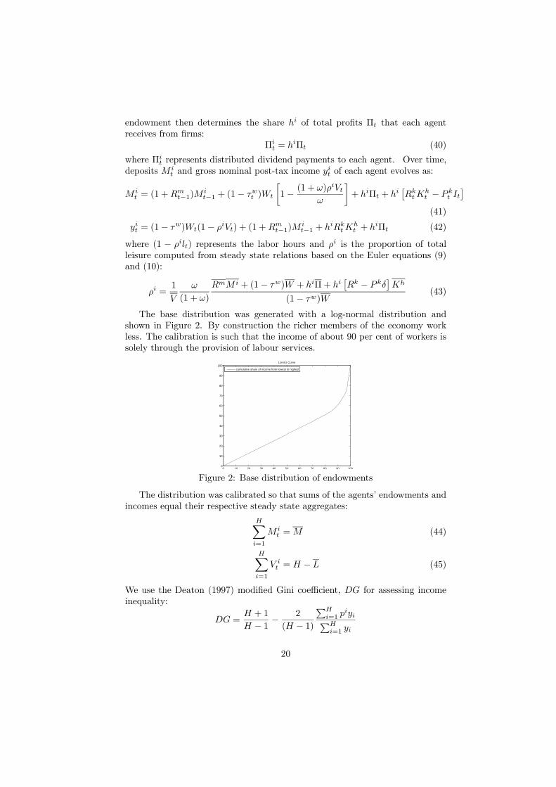
The base distribution was generated with a log-normal distribution and

shown in Figure 2. By construction the richer members of the economy work

less. The calibration is such that the income of about 90 per cent of workers is

solely through the provision of labour services.

0 10 20 30 40 50 60 70 80 90 1000

10

20

30

40

50

60

70

80

90

100Lorenz Curve

cumulative share of income from lowest to highest

Figure 2: Base distribution of endowments

The distribution was calibrated so that sums of the agents’ endowments and

incomes equal their respective steady state aggregates:

X=1

= (44)

X=1

= − (45)

We use the Deaton (1997) modified Gini coefficient, for assessing income

inequality:

= + 1

− 1 −2

( − 1)

P=1

P=1

20

where is the income rank of person , with the richest person having a rank

of 1 and the poorest person having a rank of

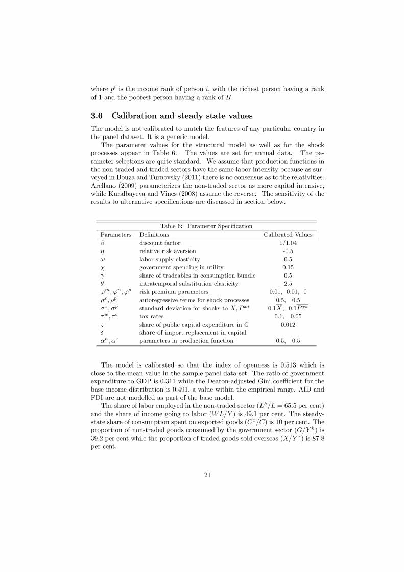
3.6 Calibration and steady state values

The model is not calibrated to match the features of any particular country in

the panel dataset. It is a generic model.

The parameter values for the structural model as well as for the shock

processes appear in Table 6. The values are set for annual data. The pa-

rameter selections are quite standard. We assume that production functions in

the non-traded and traded sectors have the same labor intensity because as sur-

veyed in Bouza and Turnovsky (2011) there is no consensus as to the relativities.

Arellano (2009) parameterizes the non-traded sector as more capital intensive,

while Kuralbayeva and Vines (2008) assume the reverse. The sensitivity of the

results to alternative specifications are discussed in section below.

Table 6: Parameter Specification

Parameters Definitions Calibrated Values

discount factor 1/1.04

relative risk aversion -0.5

labor supply elasticity 0.5

government spending in utility 0.15

share of tradeables in consumption bundle 0.5

intratemporal substitution elasticity 2.5

risk premium parameters 0.01, 0.01, 0

autoregressive terms for shock processes 0.5, 0.5

standard deviation for shocks to ∗ 0.1 0.1 ∗

tax rates 0.1, 0.05

share of public capital expenditure in G 0.012

share of import replacement in capital

parameters in production function 0.5, 0.5

The model is calibrated so that the index of openness is 0.513 which is

close to the mean value in the sample panel data set. The ratio of government

expenditure to GDP is 0.311 while the Deaton-adjusted Gini coefficient for the

base income distribution is 0491 a value within the empirical range. AID and

FDI are not modelled as part of the base model.

The share of labor employed in the non-traded sector ( = 655 per cent)

and the share of income going to labor ( ) is 49.1 per cent. The steady-

state share of consumption spent on exported goods () is 10 per cent. The

proportion of non-traded goods consumed by the government sector ( ) is

39.2 per cent while the proportion of traded goods sold overseas ( ) is 87.8

per cent.

21

4 Simulated Results

To understand better the empirical results, we first generate the impulses to

obtain insights about the key economic mechanisms following shocks that impact

on openness. In particular we shall examine the impulse responses following

shocks to trade flows (via export volume and price) as well as shocks to financial

flows (via FDI and foreign aid).

4.1 Impulse Responses

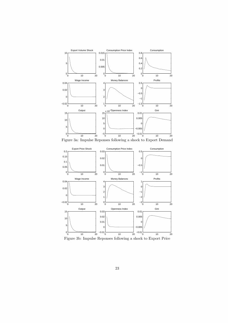
Figure 3 presents the results for the case of a shock to export demand and export

price without any foreign direct investment or foreign aid flows while Figure 4

compares the results for the Gini with and without financial flows.

4.1.1 Export Demand Shock

Figure 3a shows the impulses following a shock to the demand for exports. As

expected, the excess demand leads to an increase in the production of export

goods and upward pressure is put on the wage rate to attract more labour

into the export sector. This causes an increase in the price of home goods

and the consumption price index. The increase in the relative price of home

goods causes a switch away from the consumption of home to export goods,

resulting in an increase in aggregate consumption. Household income increases

and money balances increases. Profits falls initially because of the initial switch

away from home-goods. Overall, there is an increase in the index of openness

along with increased exports and GDP in the economy increases. The Gini

measure of inequality falls as the initial increase in wages relative to profits

causes a re-distribution in favour of those with higher labour to leisure ratios.

4.1.2 Terms of Trade Shock

Figure 3b shows the impulses following a shock to the price of export goods.

In this case, demand by the domestic sector falls, while demand by foreigners

is fixed in the model. The price of home goods and the consumption price

index rises resulting in an overall fall in consumption. Wage income increases

with more employment in the home-good sector, and money balances rises.

Returns on assets are state-dependent with risk margins falling with falls in debt.

Hence, as the value of exports increase (due to fixed demand at rising price),

debt falls and associated return on capital and hence profits fall. Meanwhile,

the index of openness improves and there is growth in the economy driven

by domestic production. The Gini measure of inequality falls as wage income

improves relative to profits.

22

0 10 200

5

10Export Volume Shock

0 10 200

0.005

0.01

0.015Consumption Price Index

0 10 200

0.2

0.4

0.6

0.8Consumption

0 10 20−0.02

0

0.02

0.04Wage Income

0 10 201

2

3

4Money Balances

0 10 20−1.5

−1

−0.5

0

0.5Profits

0 10 200

5

10

15Output

0 10 20−5

0

5

10

15x 10

−3Openness Index

0 10 20−0.01

−0.005

0

0.005

0.01Gini

Figure 3a: Impulse Reponses following a shock to Export Demand

0 10 200

0.05

0.1

0.15

0.2Export Price Shock

0 10 200

0.01

0.02

0.03Consumption Price Index

0 10 20−1

−0.5

0

0.5Consumption

0 10 20−0.02

0

0.02

0.04Wage Income

0 10 200

1

2

3

4Money Balances

0 10 20−3

−2

−1

0

1Profits

0 10 200

5

10

15Output

0 10 20−0.01

0

0.01

0.02

0.03Openness Index

0 10 20−0.01

−0.005

0

0.005

0.01Gini

Figure 3b: Impulse Reponses following a shock to Export Price

23

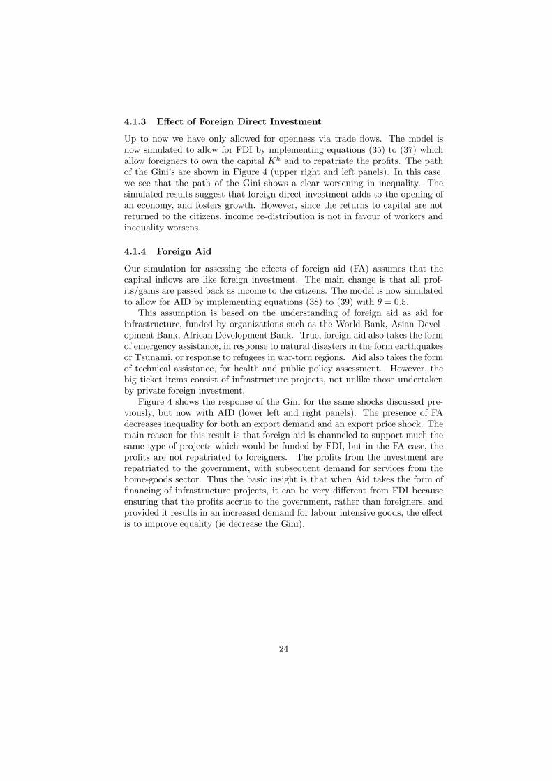
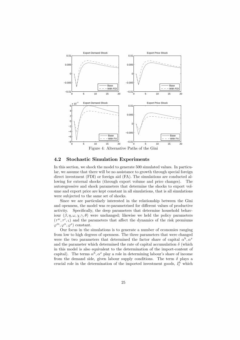
4.1.3 Effect of Foreign Direct Investment

Up to now we have only allowed for openness via trade flows. The model is

now simulated to allow for FDI by implementing equations (35) to (37) which

allow foreigners to own the capital and to repatriate the profits. The path

of the Gini’s are shown in Figure 4 (upper right and left panels). In this case,

we see that the path of the Gini shows a clear worsening in inequality. The

simulated results suggest that foreign direct investment adds to the opening of

an economy, and fosters growth. However, since the returns to capital are not

returned to the citizens, income re-distribution is not in favour of workers and

inequality worsens.

4.1.4 Foreign Aid

Our simulation for assessing the effects of foreign aid (FA) assumes that the

capital inflows are like foreign investment. The main change is that all prof-

its/gains are passed back as income to the citizens. The model is now simulated

to allow for AID by implementing equations (38) to (39) with = 05

This assumption is based on the understanding of foreign aid as aid for

infrastructure, funded by organizations such as the World Bank, Asian Devel-

opment Bank, African Development Bank. True, foreign aid also takes the form

of emergency assistance, in response to natural disasters in the form earthquakes

or Tsunami, or response to refugees in war-torn regions. Aid also takes the form

of technical assistance, for health and public policy assessment. However, the

big ticket items consist of infrastructure projects, not unlike those undertaken

by private foreign investment.

Figure 4 shows the response of the Gini for the same shocks discussed pre-

viously, but now with AID (lower left and right panels). The presence of FA

decreases inequality for both an export demand and an export price shock. The

main reason for this result is that foreign aid is channeled to support much the

same type of projects which would be funded by FDI, but in the FA case, the

profits are not repatriated to foreigners. The profits from the investment are

repatriated to the government, with subsequent demand for services from the

home-goods sector. Thus the basic insight is that when Aid takes the form of

financing of infrastructure projects, it can be very different from FDI because

ensuring that the profits accrue to the government, rather than foreigners, and

provided it results in an increased demand for labour intensive goods, the effect

is to improve equality (ie decrease the Gini).

24

0 5 10 15 20−0.01

−0.005

0

0.005

0.01Export Demand Shock

BaseWith FDI

0 5 10 15 20−0.01

−0.005

0

0.005

0.01Export Price Shock

BaseWith FDI

0 5 10 15 20−8

−6

−4

−2

0

2

4

6x 10

−3 Export Demand Shock

BaseWith FA

0 5 10 15 20−0.01

−0.005

0

0.005

0.01Export Price Shock

BaseWith FA

Figure 4: Alternative Paths of the Gini

4.2 Stochastic Simulation Experiments

In this section, we shock the model to generate 500 simulated values. In particu-

lar, we assume that there will be no assistance to growth through special foreign

direct investment (FDI) or foreign aid (FA). The simulations are conducted al-

lowing for external shocks (through export volume and price changes). The

autoregressive and shock parameters that determine the shocks to export vol-

ume and export price are kept constant in all simulations, that is all simulations

were subjected to the same set of shocks.

Since we are particularly interested in the relationship between the Gini

and openness, the model was re-parametrised for different values of productive

activity. Specifically, the deep parameters that determine household behav-

iour ( ) were unchanged; likewise we held the policy parameters

( ) and the parameters that affect the dynamics of the risk premiums

) constant.

Our focus in the simulations is to generate a number of economies ranging

from low to high degrees of openness. The three parameters that were changed

were the two parameters that determined the factor share of capital

and the parameter which determined the rate of capital accumulation (which

in this model is also equivalent to the determination of the import-content of

capital). The terms play a role in determining labour’s share of income

from the demand side, given labour supply conditions. The term plays a

crucial role in the determination of the imported investment goods, which

25

features prominently in the index of trade openness.

Φ =

∗ +

∗

= (

)( )

1−

=

¡

¢ ¡¢1−

= (1− )

−1 +

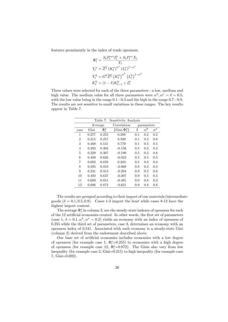
Three values were selected for each of the three parameters - a low, medium and

high value. The medium value for all three parameters were = = 05,

with the low value being in the range 01−03 and the high in the range 07−09.The results are not sensitive to small variations in these ranges. The key results

appear in Table 7.

Table 7: Sensitivity Analysis

Average Correlation parameters

case Gini Φ {Gini,Φ }

1 0.277 0.255 0.398 0.1 0.2 0.2

2 0.215 0.257 0.599 0.1 0.2 0.8

3 0.469 0.541 0.779 0.1 0.5 0.5

4 0.293 0.303 -0.156 0.5 0.2 0.2

5 0.229 0.307 -0.190 0.5 0.2 0.8

6 0.489 0.626 -0.023 0.5 0.5 0.5

7 0.692 0.859 0.383 0.5 0.8 0.8

8 0.295 0.310 -0.068 0.9 0.2 0.2

9 0.231 0.313 -0.204 0.9 0.2 0.8

10 0.492 0.637 -0.207 0.9 0.5 0.5

11 0.609 0.851 -0.491 0.9 0.8 0.2

12 0.696 0.872 -0.621 0.9 0.8 0.8

The results are grouped according to their import of raw materials/intermediate

goods ( = 01 05 09). Cases 1-3 import the least while cases 8-12 have the

highest import content.

The average Φ in column 3, are the steady-state indexes of openness for each

of the 12 artificial economies created. In other words, the first set of parameters

(case 1, = 01 = 02) yields an economy with an index of openness of

0.255 while the third set of parameters, case 3, determines an economy with an

openness index of 0.541. Associated with each economy is a steady-state Gini

(column 2) derived from the endowment described above.

Our base set of artificial economies includes economies with a low degree

of openness (for example case 1, Φ=0.255) to economies with a high degree

of openness (for example case 12, Φ=0.872). The Ginis also vary from low

inequality (for example case 2, Gini=0.215) to high inequality (for example case

7, Gini=0.692).

26

Each artificial economy is then subjected to the same set of export demand

and price shocks and the correlation between the 500 simulated Gini and open-

ness index computed. The correlations are in column 4.

Let us consider the cases with = 01 Since all three cases are subjected

to the same export demand and price shocks, the variations in openness are

generated from the variations in imports associated with the different production

structures. For these three cases, we see that the correlations with the Gini are

all positive. because the gains are small and accrue exclusively to those who are

owners of capital.

For the next 4 cases with = 05 (numbered 4-7 in Table 9), the correlation

of the Gini with the index of openness (Φ ) varies from negative to positive.

Comparing cases 5 with 2 and cases 6 with 3, we see that the economy with

the higher import-content in the capital required to produce home-goods have

negative correlations of the Gini with openness because the distribution of gains

is broader. However, a comparison of cases 6 with 7 shows that the more capital

intensive economy (case 7) actually produces a positive correlation. Since both

sectors are highly capital intensive, the distribution of income in the form of

wages (the main form of income for the majority of economic agents) is severely

limited.

For the next 5 cases with = 09 (cases 8-12), we see that the correlation of

the Gini with the index of openness (Φ ) are all negative with the largest nega-

tive value corresponding to the most open economy. In particular, comparing

cases 12 with 7 show that despite the high capital intensity in both sectors, the

economy with the higher import content in the non-traded sector, opens the

economy to more international shocks and the gains from trade are distributed

more broadly.

The same mechanisms also explain the results when we compare case 8 with

case 11, two economies with the same capital intensity in the export-sector.

However, case 8 has higher labor intensity in the non-traded sector than case

11.

For the 3 economies where the export-sector is more capital intensive then

the home-good sector ( ) (cases 2,5,9), and with similar steady-state

Ginis and Φ , the correlation of the Gini with openness becomes negative when

the import content is sufficiently large. A similar situation occurs for those

cases when production is very labour intensive in both sectors ( = = 02

cases 1,4,8); the correlation varies from positive to negative again depending on

the import-content.

These results are thus consistent with the empirical results, that the poorer

more labor intensive economies in both sectors benefit the most, in terms of

reducing inequality, from greater openness to trade. They affirm that GDP

and openness are the key factors for reducing inequality. But the correlations

vary from being strong to almost negligible and from negative to positive. In-

creasing openness, per se does not imply increasing equality. Labour intensity

in production and the nature of imported capital goods matter for the response

of inequality to increased openness.

27

5 Concluding Remarks

Our panel results show that economic growth leads unambiguously to a reduc-

tion in inequality while trade openness can increase or decrease the Gini. Foreign

direct investment and aid flows have negligible effects for low-income countries,

but they appear to benefit the middle-income countries. Overall, the panel re-

sults show why mixed results associated with trade and financial openness mute

the overall effect of globalisation on inequality.

These panel results are consistent with other empirical results reported in

the literature. However, a closer look at the data reveals that the correlations

between the Gini and openness for the countries in our sample varied from -1

to +1. To understand the variation in the correlation better, we also specified,

calibrated and simulated a stylised DSGE model of a small open economy.

We conducted simulation analysis, based on the stylized model, to help us

understand the relationship between the Gini, openness and income inequality

(impulses and correlations) along with variations in the capital intensity of the

traded and non-traded sectors.

The impulse response paths show that the key to understanding whether

trade openness, foreign direct investment and foreign aid flows have negative

or positive effects depends on the dynamics between wages and profits and the

degree of labor intensity in production. Favourable Gini outcomes come about

because of the distributive effects to wages and labour.

The analysis suggests that countries which have changed structurally to a

higher degree of openness by becoming more capital-intensive in their growing

export sector, tend to promote growth but not necessarily to promote income

equality. However, the results of this paper, both in the empirical analysis and

in the simulations, suggest that for countries where the export and home-goods

sectors are labour-intensive, growth and equality can be promoted by ensuring

that policies that favour openness also favour profit sharing.

Thus the analysis suggests that while Aid (as a percentage of donor coun-

try GDP, as emphasized by Millennium Development Goals), is ineffective, in

the first instance to promote income equality for low income countries, it ap-

pears that AID, together with trade openness, sow the seeds for growth and the

eventual alleviation of poverty.

28

References

[1] Acar, Sevil and Fatma Dogruel, 2010. Sources of inequality in selected MENA

countries. Working Paper, Marmara University, Department of Economics,

Beykoz, Turkey.

[2] Akitoby, B. Clements, S. Gupta, and G Inchauste, 2004. The Cyclical and Long-

Term Behavior of Government Expenditures in Developing Countries. IMF

Working Paper, WP/04/202.

[3] Atkinson A.B.,1970. On the measurement of inequality. Journal of Economic

Theory 2, 244-263.

[4] Anderson, Edward, 2005. Openness and inequality in developing Countres: a

review of theory and recent evidence. World Development 33, 1045-1063.

[5] Arellano, C., A. Buhlir, T. Lane, and L. Lipschitz, 2009. The dynamics impli-

cations of foreign aid and its viability. Jouran of Development Economics 88,

87-102.

[6] Barro, Robert J. and Sala-i-Martin, Xavier, 1995 Economic growth. New York:

McGraw-Hill.

[7] Basu, Parantap amd Alessandra Guarigliab, 2007. Foreign direct investment,

inequality, and growth. Journal of Macroeconomics 29, 824-839.

[8] Benabou, Roland, 1996. Inequality and growth, in Ben S Bernanke and Julio

J. Rotemberg, eds., NBER macroeconomics annual 1996. Cambridge, MA: MIT

Press, 1996b, pp. 11—74.

[9] Birdsall, Nancy; Ross, David R. and Sabot, Richard, 1995. Inequality and growth

reconsidered: lessons from East Asia. World Bank Economic Review, September

1995, 9(3), pp. 477—508.

[10] Brouza, Serpil and Stephen J. Turnovsky. 2011. The distributional consequences

of foreign transfers: do they reduce or exacterbate inequaltiy? Oxford Economic

Papers 64, 702-735.

[11] Calderón, Cecilia and Alberto Chong, 2006. Does foreign aid help reduce income

inequality? Working Paper 4437, Interamerican Development Bank.

[12] Caselli, F. and J. Ventura, 2000. A representative consumer theory of distribu-

tion. American Economic Review 90, 909-926.

[13] Chen, Yu-chin and Stephen J. Turnovsky 2010. Growth and inequality in a small

open economy. Journal of Macreconomics 32, 497-514.

[14] Correia, Isabel, 1999. On the efficiency and equity trade-off. Journal of Monetary

Economics 44, 581-603.

29

[15] Correia, Isabel. 2010. Consummption taxes and redistribution. American Eco-

nomic Review 100, 1673-1694.

[16] Daumal, Marie, 2010. The impact of trade openness on regional inequality: the

cases of India and Brazil. Working paper: Universite Paris-Dauphine.

[17] Deaton, A.,1997. Analysis of household surveys: A microeconometric approach

to development policy, Baltimore MD: Johns Hopkins University Press.

[18] Deaton, A. 2013. The great escape: health, wealth, and the origins of inequality.

Princeton, NJ: Princeton University Press.

[19] Delis, Manthos D. , Iftekar Hasan, and Nikolaos Myonidis, 2013. Foreign bank

ownership and income inequality: empirical evidence. Working Paper.

[20] Delis, Manthos D. , Iftekar Hasan and Pantelis Kazakis, 2013. Bank Regulations

and income inequality: empirical evidence. Review of Finance, forthcoming.

[21] Dollar, David and Aart Kray, 2001. Growth is good for the poor. World Bank

Working Paper 2587.

[22] Dollar, David and Aart Kraay, 2004. Trade, growth and poverty. Economic

Journal 114, F220F49.

[23] Easterly,William, 2007. Was development assistance a mistake? American Eco-

nomic Review 97, 328-332.

[24] Erlich, I, and J. Kim, 2007. The evolution of income and fertility inequalities

over the course of economic development: a human capital perspective. Journal

of Economic Growth 1, 137-174.

[25] Forbes, Kristin J., 2000. A reassessment of the relationship between inequality

and growth. American Economic Review 90(4): 869-887

[26] García-Peñalosa, Cecilia & Stephen J. Turnovsky, 2009. The dynamics Of wealth

inequality in a simple ramsey model: a note on the role of production flexibility,"

Macroeconomic Dynamics 13, 250-262.

[27] García-Peñalosa, Cecilia & Stephen J. Turnovsky, 2011. Taxation and income

distribution dynamics in a neoclassical rrowth model. Journal of Money, Credit

and Banking 43, 1543-1577,

[28] Gourdon, Julien, Micolas Maystre, and Jaime de Melo, 2008. Openness, in-

equality, and poverty: endowments matter. Journal of International Trade &

Economic Development 17, 343-378.

[29] Hirschman, Albert O. and Michael Rothschild, 1973. The chaning tolerance for

income inequaltiy in the course of economic development. The Quarterly Journal

of Economics 87, 544-566.

30

[30] Jaumotte, Florence, Subir Lall and Papageorgiou, 2008. Rising income inequal-

ity: technology or trade and financial globalization. IMFWorking Paper 08/185.

[31] Kaldor, Nicholas. 1957. A model of economic growth. Economic Journal 57,

591-624.

[32] Kuznets, Simon, 1955. Economic growth and income inequality. American Eco-

nomic Review 45, 1-28.

[33] Lim, G.C. and Paul McNelis, 2013. Alternative government spending rules: ef-

fects on income inequaltiy and welfare. Macroeconomic Dynamics, 17, 1496-1518.

[34] Majeed, M.T, 2010. Inequality, trade openness and economic growth in Asia.

Applied Econometrics and International Development 10, 201-210.

[35] Munschi, Farzana, 2012. Does openness reduce wage inequality in developing

countries? Panel data from Bangladesh. Singapore Economic Review 57, 1-12.

[36] Rudra, Nita 2004. Openness, welfare spending, and inequality in the developing

world. International Studies Quarterly 48, 683-709.

[37] Solt, F., 2009. Standardizing the world income inequality database. Social Science

Quarterly 90, 231-242.

[38] Turnovsky, Stephen. 2013. The relationship between economic growth and in-

equality. New Zealand Econoic Papers 10, 2-28.

[39] Tekin-Bouza, S. and S. Turnovsky, 2011. The distributional consequences of

foreign transfers: do they reduce or exacerbate inequality? Oxford Economic

Papers 64, 701-735

31