Embed Size (px)
Citation preview
POLITECNICO OF TURIN
Master Degree in Biomedical Engineering
Gait assessment in Parkinson’s diseaseusing waist-mounted smartphone
Supervisor : Prof.ssa Gabriella Olmo
Author : Alba Melissano
July 2019
Abstract
Parkinson’s disease (PD) is the second neurodegenerative disorder, expressed by
motor and non-motor symptoms. One of the primary motor symptoms is gait
impairment, that occurs with episodic (freezing of gait and festination) and contin-
uous disturbances, characterized by reduction of step length and gait velocity and
increase in stride-to-stride variability, that with postural instability intensifies fall
risk. Currently, to assess motor condition and gait impairment progress, subjective
and qualitative clinical evaluations are used, which may have negative effects on
diagnosis, follow-up and treatment. Therefore, gait analysis systems (laboratory-
based or laboratory-free) have been developed, providing objective and additional
information to neurologists. The aim of this study was to carry out the assessment
of PD walking, by the construction of a systems capable to detect steps, identify
initial (heel-strike) and final (toe-off) contacts of gait cycle and discriminate them
between left and right, in order to prove the feasibility of a simple and low cost sys-
tem for home monitoring of gait impairment in PD subjects. Data acquisition was
executed with a waist-mounted smartphone, which includes several inertial sensors.
A total number of 75 participants took part in the study, divided into three gro-
pus, consisting of neurological healthy people and two composed of PD subjects,
respectively. Data processing of acceleration signals was executed offline: wavelet
transform has been applied to vertical and anteroposterior components, and auto-
correlation function of vertical acceleration was computed. Spatio-temporal param-
eters and symmetry indices have been extracted and then correlated with subject
age, disease duration, UPDRS items and H&Y scores. Significance tests between
different groups have been also performed. Results were promising, with 95.3% of
total steps detected and over 85% of the parameters values in physiological ranges.
The high correlation coefficients and parameters trends are well in line with results
found in literature. The alghorithm showed good sensitivity to gait variability, ex-
pressed by step and stride variability and symmetry indices. Given the promising
results, togheter with ADL-like data aquisition, the proposed alghorithm could be
used for remote monitoring of PD patients clinical (e.g. disease progression) and
therapeutic (e.g. on/off state) condition, also in free-living environments.
ii
Acknowledgments
Desidero rivolgere un sentito ringraziamento verso la Prof.ssa Olmo e l’Ing. Borzı,
per la possibilita che mi e stata fornita nel realizzare questo lavoro e per il supporto
ricevuto.
Un doveroso ringraziamento alla mia famiglia: mamma, papa, Antonella ed Alessan-
dra, per l’estrema comprensione ed il forte incoraggiamento che mi hanno trasmesso
costantemente in questi anni, credendo sempre in me e nelle mie possibilita.
A Davide, un ringraziamento amorevole, per avermi sostenuta ed affiancata quo-
tidianamente con infinita pazienza, fornendomi utili consigli ed un luogo sicuro in
cui rifugiarmi.
A Silvia, un caloroso ringraziamento per essere stata sempre presente nonostante la
distanza, allietando con discrezione e sincero affetto le mie giornate e condividendo
a pieno questi mesi.
A Noemi, un affettuoso pensiero, per la comprensione, la delicatezza e le dolci pa-
role sempre rivoltemi durante gli anni di convivenza e non solo.
A Chiara e Clara, le mie compagne di universita nonche ormai sincere amiche, un
sentito grazie, per questi anni universitari condivisi tra gioie, difficolta, ma anche
spenzieratezza ed allegria.
Contents
Abstract . . . . . . . . . . . . . . . . . . . . . . . . . . . . . . . . . . . . ii
Acknowledgments . . . . . . . . . . . . . . . . . . . . . . . . . . . . . . . iii
List of Figures vi
List of Tables viii
1 Parkinson’s disease 1
1.1 Pathology and pathogenesis . . . . . . . . . . . . . . . . . . . . . . 1
1.2 Risk factors . . . . . . . . . . . . . . . . . . . . . . . . . . . . . . . 3
1.3 Epidemiology . . . . . . . . . . . . . . . . . . . . . . . . . . . . . . 4
1.4 Diagnosis . . . . . . . . . . . . . . . . . . . . . . . . . . . . . . . . 6
1.5 Clinical Features . . . . . . . . . . . . . . . . . . . . . . . . . . . . 7
1.5.1 A focus on gait impairment . . . . . . . . . . . . . . . . . . 9
1.6 Rating Scale . . . . . . . . . . . . . . . . . . . . . . . . . . . . . . . 13
1.6.1 Hoehn-Yahr scale . . . . . . . . . . . . . . . . . . . . . . . . 13
1.6.2 UPDRS . . . . . . . . . . . . . . . . . . . . . . . . . . . . . 13
1.6.3 Other scales . . . . . . . . . . . . . . . . . . . . . . . . . . . 14
1.7 Treatment . . . . . . . . . . . . . . . . . . . . . . . . . . . . . . . . 16
2 Gait Analysis 20
2.1 Gait Cycle . . . . . . . . . . . . . . . . . . . . . . . . . . . . . . . . 20
2.2 Gait Parameters . . . . . . . . . . . . . . . . . . . . . . . . . . . . . 21
2.3 Gait analysis . . . . . . . . . . . . . . . . . . . . . . . . . . . . . . 23
2.3.1 Laboratory-based gait analyis . . . . . . . . . . . . . . . . . 23
2.3.2 Laboratory-free gait analysis . . . . . . . . . . . . . . . . . . 25
2.4 Gait analysis in Parkinson’s disease . . . . . . . . . . . . . . . . . . 27
iv
Contents
3 Gait assessment 34
3.1 Materials . . . . . . . . . . . . . . . . . . . . . . . . . . . . . . . . 34
3.1.1 Smartphone sensors characteristics . . . . . . . . . . . . . . 34
3.1.2 Sample characteristics . . . . . . . . . . . . . . . . . . . . . 35
3.1.3 Positioning and protocol . . . . . . . . . . . . . . . . . . . . 36
3.2 Methods . . . . . . . . . . . . . . . . . . . . . . . . . . . . . . . . . 38
3.2.1 Pre-processing . . . . . . . . . . . . . . . . . . . . . . . . . . 38
3.2.2 Trunk acceleration pattern . . . . . . . . . . . . . . . . . . . 39
3.2.3 Identification of gait events: Wavelet transform . . . . . . . 41
3.2.4 Autocorrelation function . . . . . . . . . . . . . . . . . . . . 48
3.2.5 Calculation of spatio-temporal parameters and symmetry/reg-
ularity indices . . . . . . . . . . . . . . . . . . . . . . . . . . 52
3.2.6 Identification of right and left steps . . . . . . . . . . . . . . 56
3.2.7 Calculation of extra symmetry indices . . . . . . . . . . . . 62
3.2.8 Computation of Correlation Coefficients . . . . . . . . . . . 62
3.2.9 Statistical analysis: significance tests . . . . . . . . . . . . . 63
4 Results 65
4.1 Algorithm performance . . . . . . . . . . . . . . . . . . . . . . . . . 65
4.2 Correlation Coefficients - Phase 1 . . . . . . . . . . . . . . . . . . . 67
4.3 Correlation Coefficients - Phase 2 . . . . . . . . . . . . . . . . . . . 69
4.4 Significance Tests . . . . . . . . . . . . . . . . . . . . . . . . . . . . 74
4.4.1 Comparison 1: Controls vs PD subjects . . . . . . . . . . . . 74
4.4.2 Comparison 2: PD Phase 2 according to H&Y . . . . . . . . 75
4.4.3 Comparison 3: PD subjects YFOG, NFOG, HES . . . . . . 75
5 Discussion 80
6 Conclusions 86
Bibliography 88
v
List of Figures
1.1 Neuropathology of Parkinson’s disease . . . . . . . . . . . . . . . . 2
1.2 Diagram of the concept of the etiology and pathogenesis of Parkin-
son’s disease . . . . . . . . . . . . . . . . . . . . . . . . . . . . . . . 4
1.3 Incidence and prevalence of Parkinson’s disease. . . . . . . . . . . . 5
1.4 Non-motor features of Parkinson’s disease . . . . . . . . . . . . . . 10
1.5 Clinical symtoms and time course of Parkinson’s disease progression 11
1.6 Fall rates in PD compared to age-matched controls. . . . . . . . . . 12
2.1 Gait cycle phases . . . . . . . . . . . . . . . . . . . . . . . . . . . . 22
2.2 Example of marker positioning with Vicon system . . . . . . . . . . 25
2.3 Example of IMU measurements compared to Vicon system . . . . . 26
2.4 Use of two wearable sensors . . . . . . . . . . . . . . . . . . . . . . 30
2.5 Types of wereable sensors used in PD gait analysis . . . . . . . . . 31
2.6 Number of studies of smartphones and wearable sensors in neurology 31
2.7 Position of wereable sensors used in PD gait analysis . . . . . . . . 32
2.8 Acceleration obtained from two positions of sensor . . . . . . . . . . 32
3.1 Smartphone belt, smartphone position and reference axes. . . . . . 37
3.2 Frequency response of designed IIR Butterworth filter . . . . . . . . 39
3.3 Pattern of lower trunk vertical (top) and antero-posterior (bottom)
accelerations . . . . . . . . . . . . . . . . . . . . . . . . . . . . . . . 40
3.4 Mother Wavelet for AP acceleration: Gaus1 . . . . . . . . . . . . . 43
3.5 Mother Wavelet for V acceleration: Gaus1 . . . . . . . . . . . . . . 44
3.6 Wavelet transform 3D representation of AP acceleration in terms of
parameters a, b, and coefficients. . . . . . . . . . . . . . . . . . . . 45
vi
List of Figures
3.7 Wavelet transform 3D representation of V acceleration in terms of
parameters a, b, and coefficients. . . . . . . . . . . . . . . . . . . . 46
3.8 Appication of wavelet transform to AP acceleration. . . . . . . . . . 47
3.9 Appication of wavelet transform to V acceleration. . . . . . . . . . . 48
3.10 Inital contact instants detected on AP acceleration wavelet transform. 49
3.11 Final contact instants detected on V acceleration wavelet transform. 50
3.12 Superposition of anteroposterior and vertical acceleration wavelet
transforms with detected initial and final contact instants. . . . . . 51
3.13 Autocorrelation function of vertical acceleration. . . . . . . . . . . . 52
3.14 Temporal Parameters. . . . . . . . . . . . . . . . . . . . . . . . . . 56
3.15 Autocorrelation function of vertical acceleration and its regularity
coefficients. . . . . . . . . . . . . . . . . . . . . . . . . . . . . . . . 57
3.16 First method to divide steps into left and right: ML acceleration sign
at ICs istants. . . . . . . . . . . . . . . . . . . . . . . . . . . . . . . 60
3.17 Second method to divide steps into left and right: sign of ML accel-
eration area between zero-crossing of CWT AP acceleration. . . . . 61
4.1 Step Length and Gait Velocity as functions of UPDRS gait item score. 71
4.2 Step Regularity and Symmetry as functions of UPDRS gait item score. 72
4.3 Swing %GC SD, CV Stride Time, Step regularity as functions of
UPDRS postural stability item score. . . . . . . . . . . . . . . . . . 73
4.4 Cadence SD and LR Single Support %GC SD as functions of UPDRS
FOG item score. . . . . . . . . . . . . . . . . . . . . . . . . . . . . 74
4.5 Swing %GC SD and CV stance as functions of UPDRS FOG item
score. . . . . . . . . . . . . . . . . . . . . . . . . . . . . . . . . . . . 75
4.6 Step Regularity, Symmetry, Step Length and Gait Velocity as func-
tions of H&Y. . . . . . . . . . . . . . . . . . . . . . . . . . . . . . . 76
vii
List of Tables
1.1 Hoehn-Yahr Scale. . . . . . . . . . . . . . . . . . . . . . . . . . . . 13
1.2 Leg Agility, item 3.8 . . . . . . . . . . . . . . . . . . . . . . . . . . 15
1.3 Arising from chair, item 3.9 . . . . . . . . . . . . . . . . . . . . . . 15
1.4 Gait, item 3.10 . . . . . . . . . . . . . . . . . . . . . . . . . . . . . 16
1.5 Freezing of gait, item 3.11 . . . . . . . . . . . . . . . . . . . . . . . 16
1.6 Postural Stability, item 3.12 . . . . . . . . . . . . . . . . . . . . . . 17
1.7 Posture, item 3.13 . . . . . . . . . . . . . . . . . . . . . . . . . . . . 17
2.1 Comparison between advantages and disadvantages of laboratory-
based and free systems. . . . . . . . . . . . . . . . . . . . . . . . . . 28
3.1 Smartphone sensors characheristics . . . . . . . . . . . . . . . . . . 35
3.2 Control group caractheristics . . . . . . . . . . . . . . . . . . . . . . 36
3.3 Phase 1 group caractheristics . . . . . . . . . . . . . . . . . . . . . 36
3.4 Phase 2 group caractheristics . . . . . . . . . . . . . . . . . . . . . 37
3.5 Mother wavelet and scale choice. . . . . . . . . . . . . . . . . . . . 47
3.6 Quantification of the walking pattern. . . . . . . . . . . . . . . . . . 52
3.7 First differentiation errors between left and rigth steps. . . . . . . . 61
3.8 Final differentiation errors between left and right steps. . . . . . . . 62
3.9 Summary of computed spatio-temporal parameters and symmetry
indices. . . . . . . . . . . . . . . . . . . . . . . . . . . . . . . . . . . 63
4.1 Reliability of implemented method. . . . . . . . . . . . . . . . . . . 65
4.2 Difference between step time from autocorrelation function and wavelets
method. . . . . . . . . . . . . . . . . . . . . . . . . . . . . . . . . . 66
4.3 Detected physiological values . . . . . . . . . . . . . . . . . . . . . 66
viii
List of Tables
4.4 Correlation coefficients - Phase 1, Age. . . . . . . . . . . . . . . . . 67
4.5 Correlation coefficients - Phase 1, Gait Assistance. . . . . . . . . . . 68
4.6 Correlation coefficients - Phase 1, Disease Duration. . . . . . . . . . 69
4.7 Correlation coefficients - Phase 1, Gender. . . . . . . . . . . . . . . 69
4.8 Correlation coefficients - Phase 1, FOG Episodes. . . . . . . . . . . 70
4.9 Groups cardinality for each analized UPDRS item. . . . . . . . . . 70
4.10 Correlation coefficients - Phase 2, Gait Item. . . . . . . . . . . . . . 71
4.11 Correlation coefficients - Phase 2, Postural Stability Item. . . . . . 72
4.12 Correlation coefficients - Phase 2, FOG Item. . . . . . . . . . . . . . 73
4.13 Correlation coefficients - Phase 2, Arising Chair Item. . . . . . . . . 74
4.14 Correlation coefficients - Phase 2, H&Y. . . . . . . . . . . . . . . . 75
4.15 Comparison 1: Controls vs PD subjects. . . . . . . . . . . . . . . . 77
4.16 Comparison 2: PD group with H&Y=0 vs PD group with H&Y=1. 77
4.17 Comparison 2: PD group with H&Y=1 vs PD group with H&Y=2. 77
4.18 Comparison 2: PD group with H&Y=2 vs PD group with H&Y=3. 78
4.19 Comparison 2: PD group with H&Y=3 vs PD group with H&Y=4. 78
4.20 Comparison 3: PD HES vs PD YFOG. . . . . . . . . . . . . . . . . 78
4.21 Comparison 3: PD NFOG vs PD HES. . . . . . . . . . . . . . . . . 79
4.22 Comparison 3: PD NFOG vs PD YFOG. . . . . . . . . . . . . . . . 79
ix
Chapter 1
Parkinson’s disease
Parkinson’s disease (PD) is a devastating neurodegenerative pathology related to
age, with a multifactorial etiology. It owes its name to James Parkinson who
wrote in 1817 a monograph entitled ’Essay on the Shaking Palsy’. He described
with extreme details the apparent clinical signs of some patients in which an im-
balance is created between the inhibitory and excitatory mechanisms, in favor of
the latter. Excitatory (cholinergic) innervation prevails over inhibitory innerva-
tion, progressively causing a series of symptoms, such as resting tremor, hypertonia
with rigidity, akinesia, postural instability, speech and writing disorders, and also
anxiety-depressive symptoms. To date, no therapy has been found for PD, which
is cured only with symptomatic treatments.
1.1 Pathology and pathogenesis
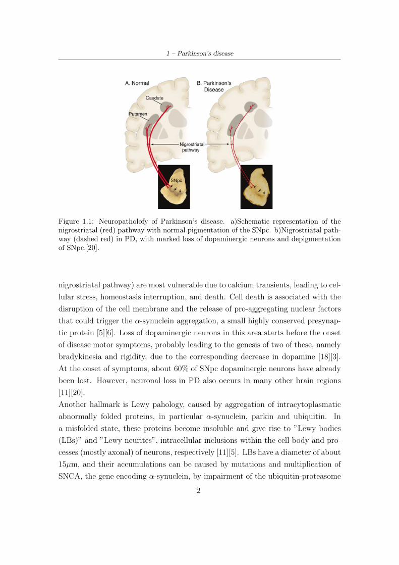
PD always show pathological hallmarks.The most important is the preferential, as
massive and progressive, degeneration of dopaminergic nigrostriatal neurons, whose
cell body is located at the level of the Substantia Nigra pars compacta (SNpc), while
the projections mainly branch towards the putamen and partly into the caudate.
The SNpc takes its name from the presence of neurons containing neuromelanine,
a dark pigment consisting of dopamine polymers (DA) embedded in a glyco-lipid
matrix. Macroscopically, the degeneration of these neurons results in the depig-
mentation of the SNpc (Fig.1.1) [20][11][18][1]. The ventrolateral cell groups (or
1
1 – Parkinson’s disease
Figure 1.1: Neuropatholofy of Parkinson’s disease. a)Schematic representation of thenigrostriatal (red) pathway with normal pigmentation of the SNpc. b)Nigrostriatal path-way (dashed red) in PD, with marked loss of dopaminergic neurons and depigmentationof SNpc.[20].
nigrostriatal pathway) are most vulnerable due to calcium transients, leading to cel-
lular stress, homeostasis interruption, and death. Cell death is associated with the
disruption of the cell membrane and the release of pro-aggregating nuclear factors
that could trigger the α-synuclein aggregation, a small highly conserved presynap-
tic protein [5][6]. Loss of dopaminergic neurons in this area starts before the onset
of disease motor symptoms, probably leading to the genesis of two of these, namely
bradykinesia and rigidity, due to the corresponding decrease in dopamine [18][3].
At the onset of symptoms, about 60% of SNpc dopaminergic neurons have already
been lost. However, neuronal loss in PD also occurs in many other brain regions
[11][20].
Another hallmark is Lewy pahology, caused by aggregation of intracytoplasmatic
abnormally folded proteins, in particular α-synuclein, parkin and ubiquitin. In
a misfolded state, these proteins become insoluble and give rise to ”Lewy bodies
(LBs)” and ”Lewy neurites”, intracellular inclusions within the cell body and pro-
cesses (mostly axonal) of neurons, respectively [11][5]. LBs have a diameter of about
15µm, and their accumulations can be caused by mutations and multiplication of
SNCA, the gene encoding α-synuclein, by impairment of the ubiquitin-proteasome
2
1 – Parkinson’s disease
system (UPS) and by corruption of the lysosomal autophagy system (LAS) [14],
which are very important for intracellular proteolysis [4][18][7][30]. Initially, α-
synuclein misfolds in a small number of cell, than gradually engages more brain
region with disease progression [14].
In PD patients brain other types of protein aggregations than α-synuclein were also
found. They synergise with Lewy pathology and contribute to the clinical expres-
sion of Parkinson’s disease. Some of these are β-amyloid plaques and tau-containing
neurofibrillary tangles, the protein inclusions typical of Alzheimer’s disease [11],
that seems to be a key factor for the cognitive decline in PD [19].
Oxidative stress is another important features of PD pathogenesis, which impli-
cates the release of oxydoradicals, eliciting the aggregation of α-synuclein and UPS
system failure [18][7]. Also mitochondrial dysfunction play a key role, leading to
both reduced ATP production and accumulation of electrons that aggrave oxidative
stress, with the final outcomes of apoptosis and cell death [18][14][7].
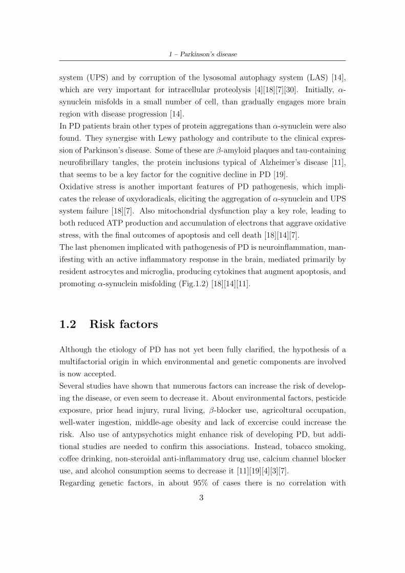
The last phenomen implicated with pathogenesis of PD is neuroinflammation, man-
ifesting with an active inflammatory response in the brain, mediated primarily by
resident astrocytes and microglia, producing cytokines that augment apoptosis, and
promoting α-synuclein misfolding (Fig.1.2) [18][14][11].
1.2 Risk factors
Although the etiology of PD has not yet been fully clarified, the hypothesis of a
multifactorial origin in which environmental and genetic components are involved
is now accepted.
Several studies have shown that numerous factors can increase the risk of develop-
ing the disease, or even seem to decrease it. About environmental factors, pesticide
exposure, prior head injury, rural living, β-blocker use, agricoltural occupation,
well-water ingestion, middle-age obesity and lack of excercise could increase the
risk. Also use of antypsychotics might enhance risk of developing PD, but addi-
tional studies are needed to confirm this associations. Instead, tobacco smoking,
coffee drinking, non-steroidal anti-inflammatory drug use, calcium channel blocker
use, and alcohol consumption seems to decrease it [11][19][4][3][7].
Regarding genetic factors, in about 95% of cases there is no correlation with
3
1 – Parkinson’s disease
Figure 1.2: Diagram of the concept of the etiology and pathogenesis of Parkinson’s disease,[18].
them, and PD is defined as ’idiopathic’ or ’sporadic’. The remaining 5% is at-
tributed to inherited genetic mutations and PD is called ’familial’. They are char-
acterized by mutations, and the most important occurs in GBA, which encodes
β-glucocerebrosidase. As already mentioned, SNCA mutation, that encodes α-
synuclein protein, leads to its aggregation and is assocated with inherited Parkin-
son’s disease. Also mutations in LRRK2 and parkin cause this type of PD, dom-
inantly and recessively respectively, and mutations in PARK7 are related to early
onset of the disease [11][15][11][19][14].
So, the risk of developing Parkinson’s disease is clearly multifactorial, and a futher
understanding of risk factors and their interactions is expected to have broad im-
plications for the elucidation of pathogenic mechanism and individualisation of
treatment [11].
1.3 Epidemiology
Parkinson’s disease is the second most common neurodegenerative disorder after
Alzheimer. It is mainly an illness of later life, so is more common in developed
4
1 – Parkinson’s disease
countries where people live longer [7]. The estimated prevalence of PD in indus-
trialized countries is 0.3% in the general population, 1.0% in people older than
60 years, and 3.0% in those aged 80 years and older, with incidence rates of 8 to
18 per 100000 person-years [8]. In Europe the prevalence at age between 85 and
89 has been reported as 3.5% [9] and in Italy the estimated average prevalence
is 157,7/100000 [10]. Both incidence and prevalence increase nearly exponentially
with advancing age [11]. So with an aging population and rising life expectancy
worldwide, the number of people with PD is expected to increase by more than 50%
by 2030 [12]. Moreover, the incidence seems to vary within subgroups definded by
race and ethnicity. In particular it seems be greater in Hispanics, followed by non-
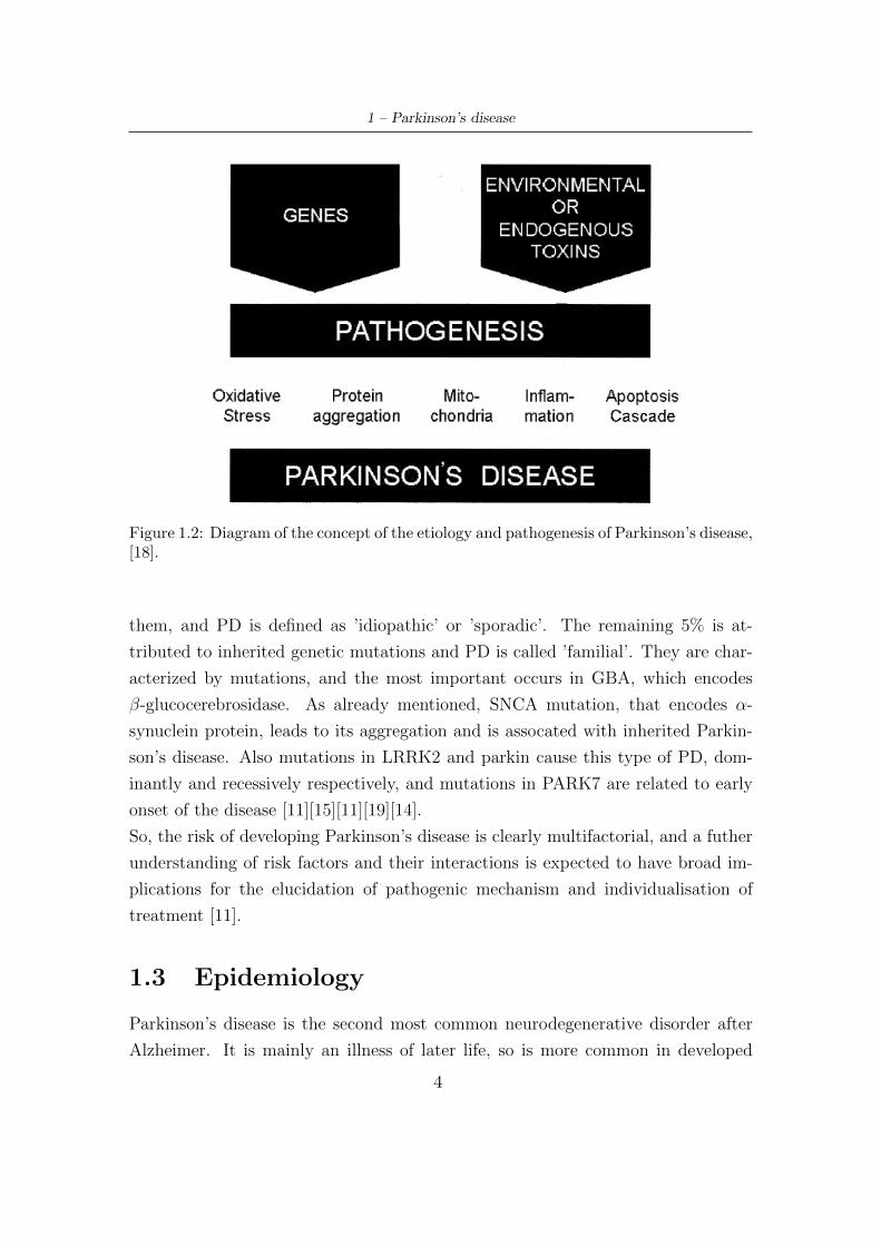
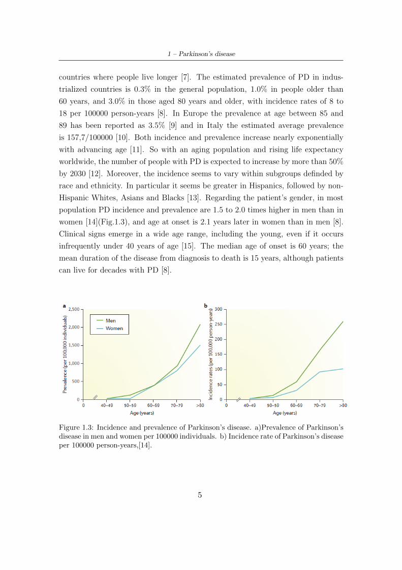
Hispanic Whites, Asians and Blacks [13]. Regarding the patient’s gender, in most
population PD incidence and prevalence are 1.5 to 2.0 times higher in men than in
women [14](Fig.1.3), and age at onset is 2.1 years later in women than in men [8].
Clinical signs emerge in a wide age range, including the young, even if it occurs
infrequently under 40 years of age [15]. The median age of onset is 60 years; the
mean duration of the disease from diagnosis to death is 15 years, although patients
can live for decades with PD [8].
Figure 1.3: Incidence and prevalence of Parkinson’s disease. a)Prevalence of Parkinson’sdisease in men and women per 100000 individuals. b) Incidence rate of Parkinson’s diseaseper 100000 person-years,[14].
5
1 – Parkinson’s disease
1.4 Diagnosis
The evaluation of PD is difficult because the expression of the disorder varies from
patient to patient (intra-patient variability), and is also significantly influenced by
emotional state, response to drugs, and other variables [17]. Hovewer, the diagnosis
of PD is still largely a clinical one, as there is no definitive test able to confirm the
diagnosis during life [15][16]. From a practical perspective, the first step for the
diagnosis of PD is a careful analysis of patient’s history. In particular, in-depth
investigations must be carried out, trying to define emerged symptoms and their
sequence (such as premotor symptoms), to analyze if patient is exposed to en-
vironmental risk factors, to record past and present medical impairments and to
examine possible neurological disorders in other family members [15]. At this point,
careful clinical examination follows. The disease is clinically defined by presence of
bradykinesia and at least one additional cardinal motor feature (rigidity and/or rest
tremor), additional supporting and exclusionary criteria, and response to levodopa.
The latter is very helpful, indicating presynaptic dopamine deficiency with intact
postsynaptic dopamine receptors, features typical of PD [18]. The clinical findings
are usually asymmetrical and remain the same throughout the disease, with gait
and balance affected later [15][18][4][14][19][16][11].
There are no practical diagnostic laboratory tests for PD, and in most cases, the
diagnosis is made only with these clinical examinations, but in specific circum-
stances, other ancillary investigations are needed. Imaging techniques are used
to differentiate Parkinson’s disease with motor symptoms from disorders without
presynaptic dopaminergic terminal deficiency [11]. Positron emission tomography
(PET) with fluorodopa (FDOPA) is one of the available technologies, that mea-
sures levodopa uptake into dopamine nerve terminals, but the costs and limited
accessibility make it difficult to use [15][18]. Dopamine transporter (DAT) imaging
with single photon emission computed tomografy (SPECT) is also a very useful ap-
proach, because it is sensitive for the detection of presynaptic dopaminergic neuron
degeneration in the striatum [11][15]. Brain structural imaging, either by computed
tomography (CT) or magnetic resonance imaging (MRI) can be performed, where
the latter is preferred [15]. Standard MRI has a marginal role in PD diagnosis,
but high and ultra-high-field MRI combined with advanced techniques are used to
6
1 – Parkinson’s disease
enhance diagnostic accuracy for Parkinson’s disease versus other types of degener-
ative parkinsonism [11][14].
Genetic testing is not part of the routine diagnostic process, except in patients in
whom there is a specific suspicion for a possible genetic cause (for example sugges-
tive family history and early onset) [14][11]. Although several studies have assessed
α-synuclein and other proteins concentrations in cerebrospinal fluid (CSF), there is
currently no clinically useful CSF-based diagnostic test for PD. This is also true for
blood biomarkers, although associations of different serum or plasma parameters
with disease progression have been described [14][11].
1.5 Clinical Features
The clinical expressions of Parkinson’s disease can be divided into two categories:
motor symptoms and non-motor symptoms.
The onset of motor symptoms is usually unilateral and asymmetry persists through-
out the disease, even in advanced stage. From this standpoint, PD is characterized
by four cardinal features [14][7]:
� Bradykinesia. It is the most characteristic clinical feature of PD, and it refers
to slowness of movement. It may be manifested by a delay in the initiation
of a movement and by slowness of its execution. Other aspects include a de-
lay in arresting movement, amplitude and speed decrementing of repetitive
movements, and inability to execute simultaneos or sequential actions. In ad-
dition to whole body slowness and impairment of fine motor movement, other
manifestations of bradykinesia involve drooling due to impaired swallowing
of saliva, monotonous dysarthria, loss of facial expression (hypomimia), re-
duced arm swing when walking (loss of automatic movement), micrographia,
reduced amplitude of voice and decreased stride length during walking. Its
clinical assessment is carried out by globally observing the patient’s sponta-
neous movements while sitting or walking, and asking him to perform some
repetitive movements in a wide and fast way, such as opening and closing the
hand, tapping the foot on the ground. During these tasks the examiner looks
for a possible decrease or loss in the amplitude.[15][16][17][18][20][7].
� Rest tremor, that is the most common and easily recognised symptom of PD.
7
1 – Parkinson’s disease
It is defined as a rythmic oscillatory involuntary movement that comes about
when the affected body part is relaxed. It is unilateral, but over time it can
affect both sides. Characteristically, rest tremor disappears or decreases its
intensity as soon as a finalized movement is performed to execute a certain
actions, and during sleep [15][16]. Commonly, this motor symptom manifests
as a resting ”pill-rolling” hand tremor, that is a supination-pronation tremor
which might be evident when the patient is asked to do fine finger movements
with the other hand or to walk. Occasionally it involves legs, jaw and tongue,
whereas head tremor is not typical of PD [9][15][19]. It occurs at a frequency
between 4 and 6 Hz, and can be intermittent at the beginning, being present
only in stressful and anxious situations, but with the progression of the disease
it tends to be present most of the time and worsen in amplitude with stress
or excitement [18][7]. In clinical practice, tremor is observed when the limb
muscles are relaxed, elicited by patient’s focus on a particular mental task,
such as countdown with eyes closed [15].
� Rigidity. It indicates an increase in muscle tone at rest or during movement,
and is characterized by an increase in resistance during passive mobilization of
an extremity, independent of direction and velocity of movement [48]. Rigidity
can affect limbs, neck and trunk and appears in several daily activities, like
dressing, writing and turning in bed. Typically, during examination of a seg-
ment, it is increased by voluntary movement of other body parts (Froment’s
maneuver) [15][16][7].
� Postural and gait impairment. They include postural instability and parkinso-
nian gait. Postural instability occurs mainly in advanced stages of PD and is
caused by a reduction in straightening reflexes, so that subject is not able to
spontaneously correct imbalances or to maintain an upright posture. There-
fore the patient is more subject to falls (often resulting in hip fractures) which
can occur in all directions even if more frequently forward. As the disease
progresses, the subject assumes a stooped posture, in which the trunk is bent
forward, arms are kept close to trunk and bent, as knees. In the later stages
it is also possible to appreciate permanent curvature of neck and back. Clini-
cally, it is evaluated by the pull test: the examiner stands behind the patient
and applies a pull in order to assess the ability to regain balance.
8
1 – Parkinson’s disease
Parkinsonian gait is slow and hypokinetic, occurs on a narrow base, and is
characterized by short shuffling steps and reduced step length, which gives the
observer the impression that the patient is chasing own center of gravity. An-
other gait disturbance than shuffling is motor blocking, that is called freezing
of gait[9][15][17].
There are many other motor findings in PD, most of which are directly related to
one of cardinal signs [17].
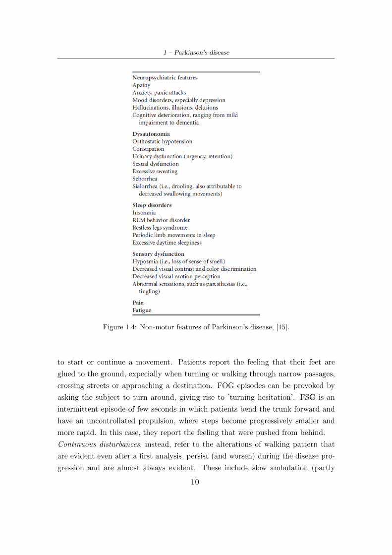
Although the motor symptoms of PD dominate the clinical picture, parkinsonian
subjects also present several non-motor symptoms (Fig.1.4). These include sen-
sory complaints, cognitive impairment, psychiatric symptoms, sleep disorders, au-
tonomic dysfunction, pain and fatigue [11][16][18]. Frequently, some of these can
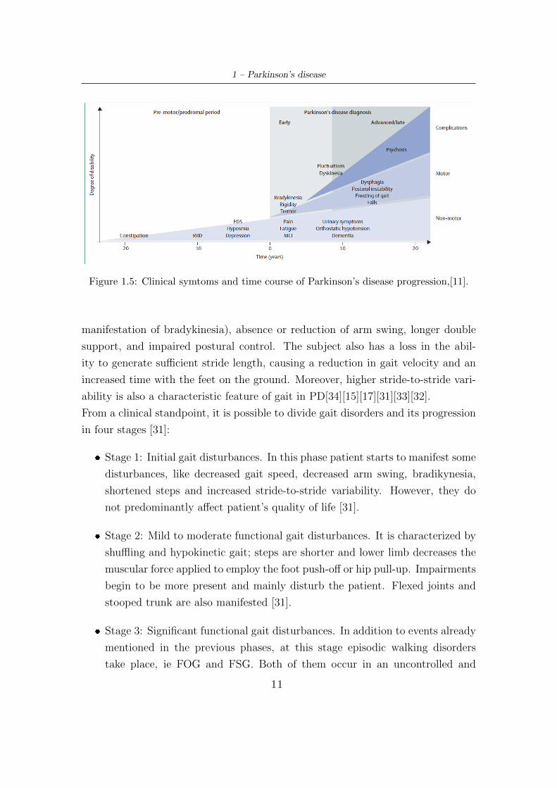
anticipate the onset of classic motor symptoms by years or even decades [15][14][7],
such as impaired olfaction, constipation, depression, excessive daytime sleepiness
(EDS), and rapid eye movement sleep behavior disorder (RBD)(Fig.1.5). This pe-
riod is called premotor or prodromal phase [11], and its features vary from patient
to patient [9]. With the disease progression, worsening of motor features occurs,
and there is an emergence of complications related to long-term symptomatic treat-
ment, including motor and non-motor fluctuations, dyskinesia (abnormal involun-
tary movement) and psychosis [11]. Severity of bradykinesia, rigidity, gait and
balance progress similarly, while tremor severity appears to be rather stable over
time, possibly indicating different underlying pathophysiological processes [7].
1.5.1 A focus on gait impairment
Gait disorders in PD is caused by imbalance of cortical and subcortical activities
with inhibition of the primary motor cortex, putamen, and cerebellum, which are
replaced by overactivation of non-typical brain areas. Some factors that contribute
to damage gait are a decrease in the senses of proprioception, discrimination, and
position.
Gait impairments can be divided into two types: continuous and episodic. Episodic
disturbances have a random, intermittent and unpredictable nature. These include
freezing of gait (FOG), festination gait (FSG), and start hesitation. FOG occurs
most often in PD patient who are in an advanced state of the disease. It is a
form of akinesia (loss of movement) and consists of a sudden and transient inability
9
1 – Parkinson’s disease
Figure 1.4: Non-motor features of Parkinson’s disease, [15].
to start or continue a movement. Patients report the feeling that their feet are
glued to the ground, expecially when turning or walking through narrow passages,
crossing streets or approaching a destination. FOG episodes can be provoked by
asking the subject to turn around, giving rise to ’turning hesitation’. FSG is an
intermittent episode of few seconds in which patients bend the trunk forward and
have an uncontrollated propulsion, where steps become progressively smaller and
more rapid. In this case, they report the feeling that were pushed from behind.
Continuous disturbances, instead, refer to the alterations of walking pattern that
are evident even after a first analysis, persist (and worsen) during the disease pro-
gression and are almost always evident. These include slow ambulation (partly
10
1 – Parkinson’s disease
Figure 1.5: Clinical symtoms and time course of Parkinson’s disease progression,[11].
manifestation of bradykinesia), absence or reduction of arm swing, longer double
support, and impaired postural control. The subject also has a loss in the abil-
ity to generate sufficient stride length, causing a reduction in gait velocity and an
increased time with the feet on the ground. Moreover, higher stride-to-stride vari-
ability is also a characteristic feature of gait in PD[34][15][17][31][33][32].
From a clinical standpoint, it is possible to divide gait disorders and its progression
in four stages [31]:
� Stage 1: Initial gait disturbances. In this phase patient starts to manifest some
disturbances, like decreased gait speed, decreased arm swing, bradikynesia,
shortened steps and increased stride-to-stride variability. However, they do
not predominantly affect patient’s quality of life [31].
� Stage 2: Mild to moderate functional gait disturbances. It is characterized by
shuffling and hypokinetic gait; steps are shorter and lower limb decreases the
muscular force applied to employ the foot push-off or hip pull-up. Impairments
begin to be more present and mainly disturb the patient. Flexed joints and
stooped trunk are also manifested [31].
� Stage 3: Significant functional gait disturbances. In addition to events already
mentioned in the previous phases, at this stage episodic walking disorders
take place, ie FOG and FSG. Both of them occur in an uncontrolled and
11
1 – Parkinson’s disease
unpredictable way, and have a temporal duration of seconds, rarely exceeding
30s.
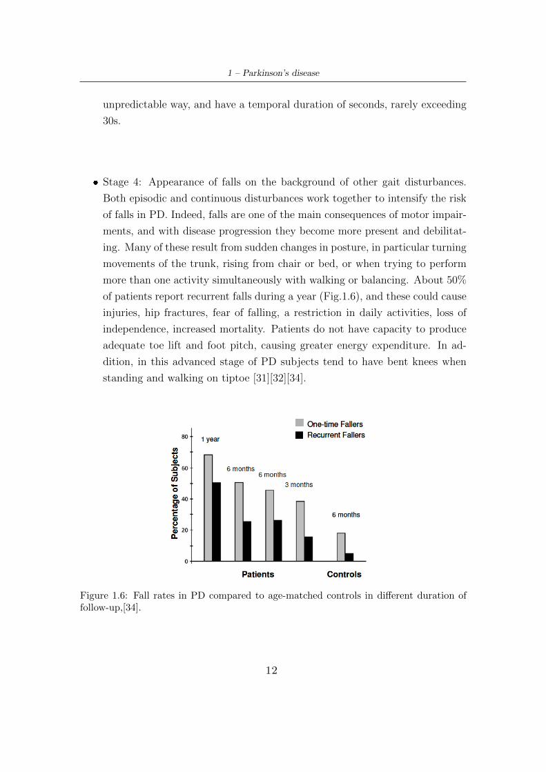
� Stage 4: Appearance of falls on the background of other gait disturbances.
Both episodic and continuous disturbances work together to intensify the risk
of falls in PD. Indeed, falls are one of the main consequences of motor impair-
ments, and with disease progression they become more present and debilitat-
ing. Many of these result from sudden changes in posture, in particular turning
movements of the trunk, rising from chair or bed, or when trying to perform
more than one activity simultaneously with walking or balancing. About 50%
of patients report recurrent falls during a year (Fig.1.6), and these could cause
injuries, hip fractures, fear of falling, a restriction in daily activities, loss of
independence, increased mortality. Patients do not have capacity to produce
adequate toe lift and foot pitch, causing greater energy expenditure. In ad-
dition, in this advanced stage of PD subjects tend to have bent knees when
standing and walking on tiptoe [31][32][34].
Figure 1.6: Fall rates in PD compared to age-matched controls in different duration offollow-up,[34].
12
1 – Parkinson’s disease
1.6 Rating Scale
In assessing the motor and non-motor symptoms, signs and disabilities of PD, rat-
ing scale are used to quantify the impairment and assign a value to a particular
features or symptom in question [17][16][2]. Motor scales are the best-known and
most widely used, but non-motor symptom scales are equally important. Combined
with a motor scale, these give a more balanced picture of how a person is affected
by disease [2].
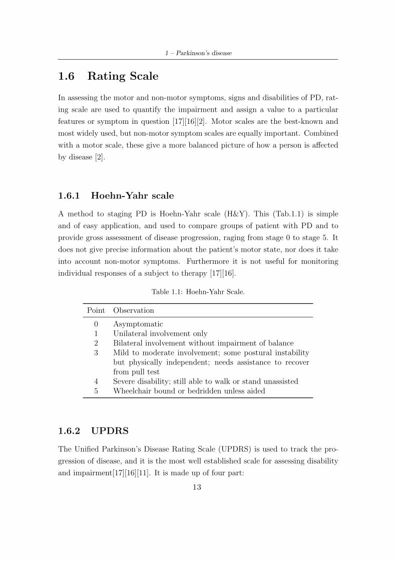
1.6.1 Hoehn-Yahr scale
A method to staging PD is Hoehn-Yahr scale (H&Y). This (Tab.1.1) is simple
and of easy application, and used to compare groups of patient with PD and to
provide gross assessment of disease progression, raging from stage 0 to stage 5. It
does not give precise information about the patient’s motor state, nor does it take
into account non-motor symptoms. Furthermore it is not useful for monitoring
individual responses of a subject to therapy [17][16].
Table 1.1: Hoehn-Yahr Scale.
Point Observation
0 Asymptomatic1 Unilateral involvement only2 Bilateral involvement without impairment of balance3 Mild to moderate involvement; some postural instability
but physically independent; needs assistance to recoverfrom pull test
4 Severe disability; still able to walk or stand unassisted5 Wheelchair bound or bedridden unless aided
1.6.2 UPDRS
The Unified Parkinson’s Disease Rating Scale (UPDRS) is used to track the pro-
gression of disease, and it is the most well established scale for assessing disability
and impairment[17][16][11]. It is made up of four part:
13
1 – Parkinson’s disease
� Part I: Evaluation of mental activity, behaviour and mood.
� Part II: Self-evaluation of activities of daily living.
� Part III: Evaluation of motor function.
� Part IV: Evaluation of complications of therapy.
Each part involves several items to appointing a value to a particular features.
The UPDRS testing is carried out by a healthcare professional. Points assigned to
every item are based on the person’s response, as well as observation and physical
examination, and range from 0 to 4. The total cumulative score ranges from 0
(no disability) to 199 (total disability). The scale was introduced in 1987 and has
since been updated by specialists from the Movement Disorder Society (MDS) to
include new assessments of non-motor symptoms [2]. The UPDRS is often used
with H&Y scale, and the Schwab and England Activities of Daily Living (ADL)
Scale. Relating to Part III of UPDRS scale, items more inherent to this document
are:
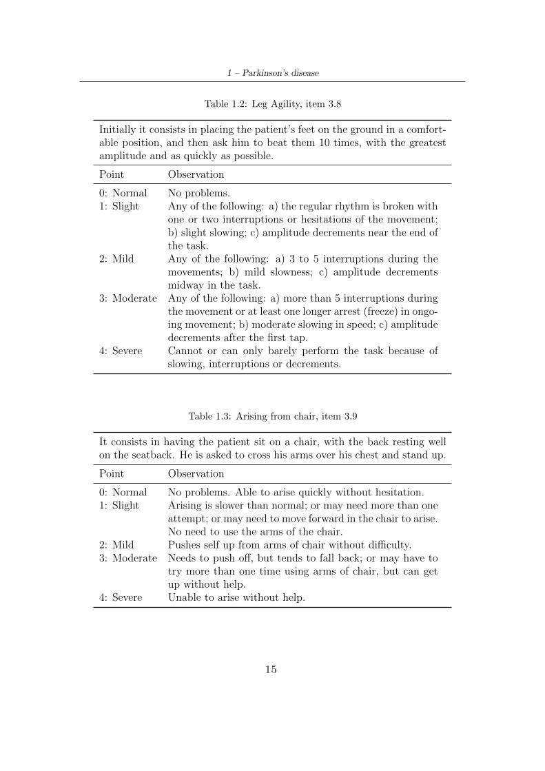
� ’Leg Agility (3.8)’, Tab.1.2.
� ’Arising from Chair (3.9)’, Tab.1.3.
� ’Gait (3.10)’, Tab.1.4.
� ’Freezing of gait (3.11)’, Tab.1.5.
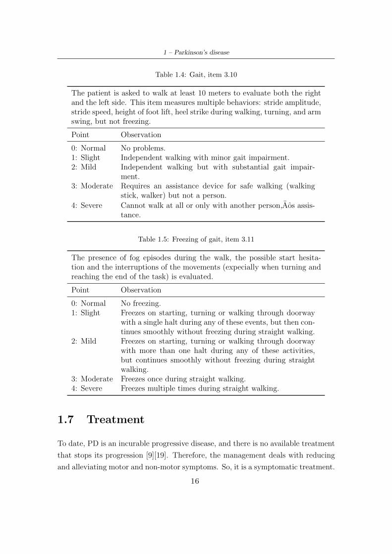
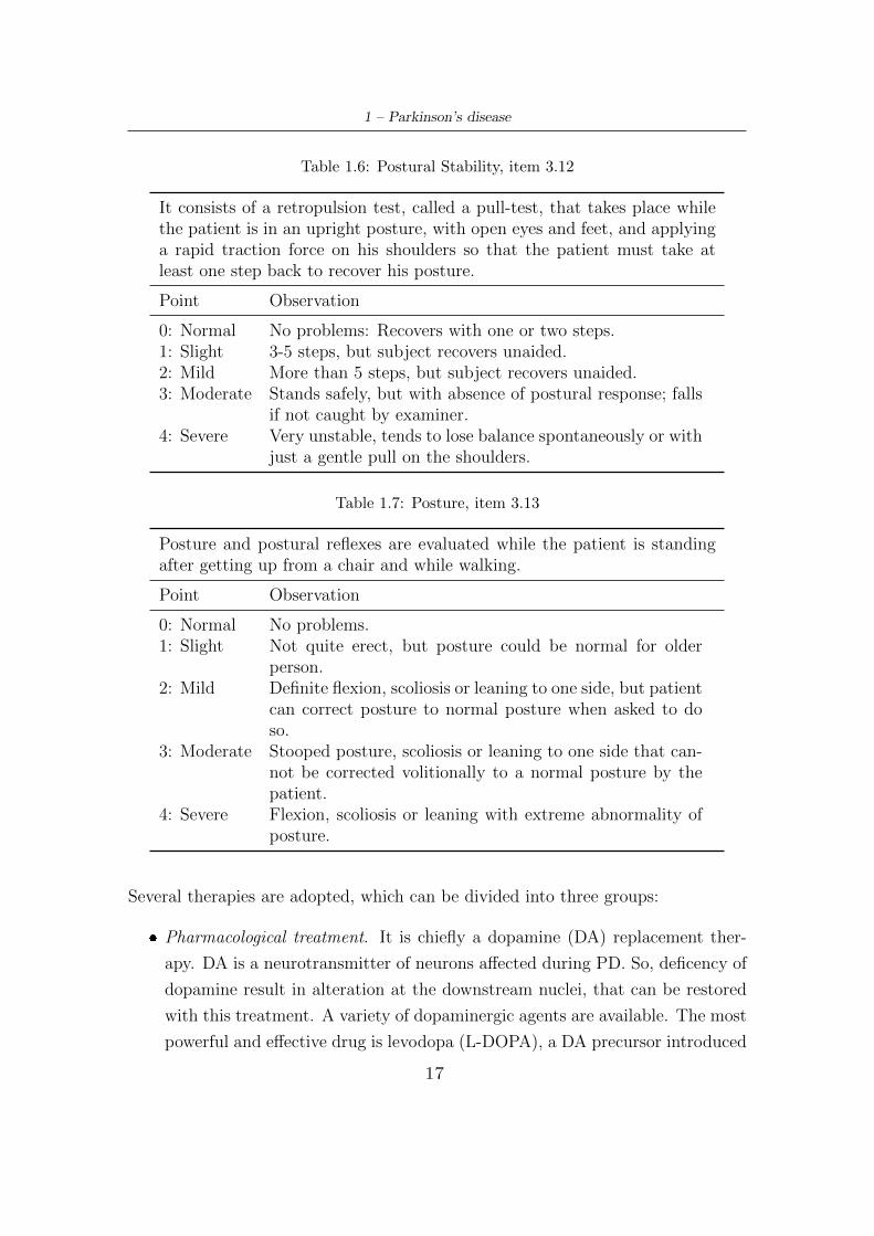
� ’Postural Stability (3.12)’, Tab.1.6.
� ’Posture (3.13)’, Tab.1.7.
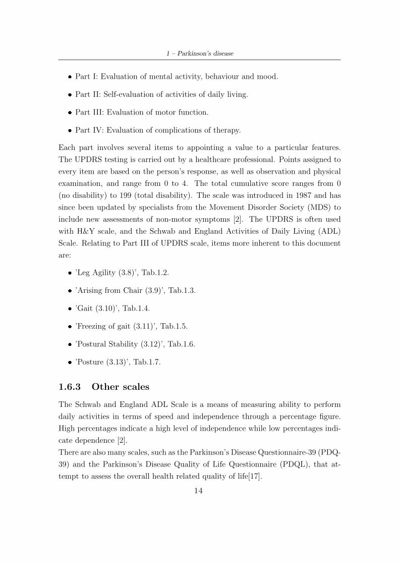
1.6.3 Other scales
The Schwab and England ADL Scale is a means of measuring ability to perform
daily activities in terms of speed and independence through a percentage figure.
High percentages indicate a high level of independence while low percentages indi-
cate dependence [2].
There are also many scales, such as the Parkinson’s Disease Questionnaire-39 (PDQ-
39) and the Parkinson’s Disease Quality of Life Questionnaire (PDQL), that at-
tempt to assess the overall health related quality of life[17].
14
1 – Parkinson’s disease
Table 1.2: Leg Agility, item 3.8
Initially it consists in placing the patient’s feet on the ground in a comfort-able position, and then ask him to beat them 10 times, with the greatestamplitude and as quickly as possible.
Point Observation
0: Normal No problems.1: Slight Any of the following: a) the regular rhythm is broken with
one or two interruptions or hesitations of the movement;b) slight slowing; c) amplitude decrements near the end ofthe task.
2: Mild Any of the following: a) 3 to 5 interruptions during themovements; b) mild slowness; c) amplitude decrementsmidway in the task.
3: Moderate Any of the following: a) more than 5 interruptions duringthe movement or at least one longer arrest (freeze) in ongo-ing movement; b) moderate slowing in speed; c) amplitudedecrements after the first tap.
4: Severe Cannot or can only barely perform the task because ofslowing, interruptions or decrements.
Table 1.3: Arising from chair, item 3.9
It consists in having the patient sit on a chair, with the back resting wellon the seatback. He is asked to cross his arms over his chest and stand up.
Point Observation
0: Normal No problems. Able to arise quickly without hesitation.1: Slight Arising is slower than normal; or may need more than one
attempt; or may need to move forward in the chair to arise.No need to use the arms of the chair.
2: Mild Pushes self up from arms of chair without difficulty.3: Moderate Needs to push off, but tends to fall back; or may have to
try more than one time using arms of chair, but can getup without help.
4: Severe Unable to arise without help.
15
1 – Parkinson’s disease
Table 1.4: Gait, item 3.10
The patient is asked to walk at least 10 meters to evaluate both the rightand the left side. This item measures multiple behaviors: stride amplitude,stride speed, height of foot lift, heel strike during walking, turning, and armswing, but not freezing.
Point Observation
0: Normal No problems.1: Slight Independent walking with minor gait impairment.2: Mild Independent walking but with substantial gait impair-
ment.3: Moderate Requires an assistance device for safe walking (walking
stick, walker) but not a person.
4: Severe Cannot walk at all or only with another person’Aos assis-
tance.
Table 1.5: Freezing of gait, item 3.11
The presence of fog episodes during the walk, the possible start hesita-tion and the interruptions of the movements (expecially when turning andreaching the end of the task) is evaluated.
Point Observation
0: Normal No freezing.1: Slight Freezes on starting, turning or walking through doorway
with a single halt during any of these events, but then con-tinues smoothly without freezing during straight walking.
2: Mild Freezes on starting, turning or walking through doorwaywith more than one halt during any of these activities,but continues smoothly without freezing during straightwalking.
3: Moderate Freezes once during straight walking.4: Severe Freezes multiple times during straight walking.
1.7 Treatment
To date, PD is an incurable progressive disease, and there is no available treatment
that stops its progression [9][19]. Therefore, the management deals with reducing
and alleviating motor and non-motor symptoms. So, it is a symptomatic treatment.
16
1 – Parkinson’s disease
Table 1.6: Postural Stability, item 3.12
It consists of a retropulsion test, called a pull-test, that takes place whilethe patient is in an upright posture, with open eyes and feet, and applyinga rapid traction force on his shoulders so that the patient must take atleast one step back to recover his posture.
Point Observation
0: Normal No problems: Recovers with one or two steps.1: Slight 3-5 steps, but subject recovers unaided.2: Mild More than 5 steps, but subject recovers unaided.3: Moderate Stands safely, but with absence of postural response; falls
if not caught by examiner.4: Severe Very unstable, tends to lose balance spontaneously or with
just a gentle pull on the shoulders.
Table 1.7: Posture, item 3.13
Posture and postural reflexes are evaluated while the patient is standingafter getting up from a chair and while walking.
Point Observation
0: Normal No problems.1: Slight Not quite erect, but posture could be normal for older
person.2: Mild Definite flexion, scoliosis or leaning to one side, but patient
can correct posture to normal posture when asked to doso.
3: Moderate Stooped posture, scoliosis or leaning to one side that can-not be corrected volitionally to a normal posture by thepatient.
4: Severe Flexion, scoliosis or leaning with extreme abnormality ofposture.
Several therapies are adopted, which can be divided into three groups:
� Pharmacological treatment. It is chiefly a dopamine (DA) replacement ther-
apy. DA is a neurotransmitter of neurons affected during PD. So, deficency of
dopamine result in alteration at the downstream nuclei, that can be restored
with this treatment. A variety of dopaminergic agents are available. The most
powerful and effective drug is levodopa (L-DOPA), a DA precursor introduced
17
1 – Parkinson’s disease
in therapy at the end of the 60s. It is usually administered with two inhibitors:
a decarboxylase inhibitor to prevent formation in the peripheral tissues, and
catechol-O-methyltransferase inhibitor to extend its plasma half-life and to
prolong the duration of action of each dose [18]. However, after some years,
the use of L-DOPA is complicated by the evolution of shorter duration of re-
sponse to individaul doses (wearing off symptoms), alternative phases with
good and poor response to medication (on-off symptoms), drug-induced invol-
untary movement of the head, trunk or limbs (dyskinesias), and psychosis [14]
[18][19][15][9][11].
A very advantageous approach to maintain constant levodopa plasma con-
centrations is the administration of a levodopa-carbidopa concentrate in the
duodenum (known as Duodopa) through a percutaneous endogastric tube con-
nected to a portable infusion pump. This pump allows adjustment of the drug
dose according to the patient’s condition. This approach has partly reduced
the dyskinesias typical of the advanced stages of PD. Furthermore, even a
subcutaneous infusion of apomorphine (a powerful antagonist of DA) leads to
an improvement in motor fluctuations.
Moreover, in the last few months, a new drug has been marketed: Ongentys,
also known as Opicapone. This is an inhibitor of COMT enzymes that degrade
L-DOPA at the peripheral level. Therefore it allows to increase the amount of
absorbed L-DOPA, reducing motor fluctuations at the end of the dose. So, it
is administered only to patients already treated with L-DOPA.
Other drugs used in treating PD symptoms are dopamine agonists. They have
good efficacy, and compared to L-DOPA are less likely to produce motor com-
plications, but are more likely to cause hallucinations, confusion and psychosis,
and provide less symptomatic benefit. So, thery are not recommended to el-
derly over age of 70 years [18][15][14]. Subjects with PD also use dopamine
releaser, like amantadine, that relieves symtoms (also dyskinesia) but produces
mental effects, and monoamine oxidase type B (MAO-B) inhibitors [18][14].
The efficacy of each of these drugs, as well as their adverse-event, need to be
fully explained to the patient when treatment options are being considered,
and seems to be also influenzed by placebo response [19].
There are also nondopaminergic agents that are useful to treat L-DOPA re-
sistant (”non-dopaminergic”) features (treatment-resistant tremor, freezing of
18
1 – Parkinson’s disease
gait, postural instability, falls, swallowing and speech disturances), but also
non-motor features, like cognitive and psychotic defects [18][14].
� Surgical treatment. It is characterized by stereotaxic deep brain stimulation
(DBS), that can be unilateral and bilater. It is made up of a neurostimulator,
that is placed subcutaneously in the anterior and superior region of the thorax,
and an electrode positioned in the brain. Once the system is in loco, electri-
cal impulses sent from the generator into the brain reduce abnormal electrical
signals and alleviate PD motor symptoms. It is used when patient have ad-
vanced PD with an excellent L-DOPA response but also motor complications
due to long-term medical treatment. The average time to surgical treatment is
about after 10-13 years after diagnosis of PD, and location needs to be individ-
ualized for each patient. However, treatment of subthalamic nucleus (STN)
reduce bradykinesia and levodopa dosage, and therefore dyskinesia severity
[18] [15][9][11]. It can also alleviate gait impairment and postural instability,
improving asymmetry of gait and joints range of motion, and increasing step
length and velocity [31]. Moreover, targeted gene therapy and cell transplan-
tation are also included in this group [11].
� Exercise-based treatment, which seem to improve symptoms that do not re-
spond to pharmacological and surgical therapies, like mobility, postural con-
trol and balance. This consist of physical therapy with cueing to improve gait,
excercise to improve balance, training to build up muscle power and increase
joint mobility [19][14].
19
Chapter 2
Gait Analysis
2.1 Gait Cycle
Walking can be defined as ”a method of locomotion involving the use of the two
legs, alternatly, to provide both support and propulsion”. Formally, walking uses a
ripetitious sequence of limb motion to move the body forward while simultaneosuly
maintaing stance stability [21].
Human walking is identified by gait cycle cyclical sequence. Gait cycle (GC) is
characterized by so-called gait events, that are defined on the basis of feet contact
with the ground. They are:
� Heel Strike (HS): the impact of the heel on the ground, ie represents the
beginning of load phase, also referred as initial contact (IC). However, for a
pathological gait it is possible that either the toe, side of a foot or even the
whole foot first touches the ground rather than heel [44].
� Toe-Strike (TS): the impact of the toe on the ground and it represents the end
of load phase.
� Heel-Off (HO): the detachment of the heel from the ground; it starts the push
phase.
� Toe-Off (TO): the detachment of the toe from the ground; it concludes the
push phase, also referred as final contact (FC).
20
2 – Gait Analysis
GC is the time interval between two successive and repetitive events of ipsilateral
foot (on the same side of the body). It is considered to begin from the contact of
one foot with ground (IC) and to finish with next same foot contact. So, gait cycle
consists of two steps: left and right. The step begins with the contact of ipsilateral
foot and ends with that of contralateral (other side of the body) foot. The sequence
of the steps (left-right or right-left) depends on the person’s first step.
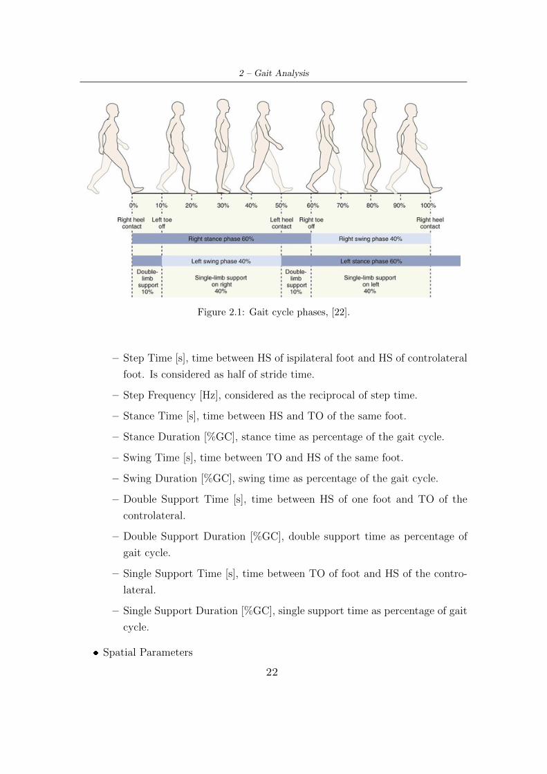
It is divided in two phases: stance phase and swing phase (Fig.2.1), that are defined
by gait events. The stance indicates the period during which the foot of considered
lower limb lies on the ground, so begins with the heel-strike (IC) and ends with
the toe-off (FC) . The swing, on the contrary, refers to the period in which foot
is in the air for the limb advancement, begins with TO and ends with a new heel-
strike. Usually, during normal walking, their physiological values are about 60%
and 40% of GC, for stance phase and swing phase respectively. However, these
vary according to walking speed: if velocity increases, stance becomes smaller and
the swing increases [47]. Moreover, GC can be divided in two other phases: single
support and double support. The first occurs when leg is in swing phase and the
other is in stance, therefore body weight is supported by a single limb. It starts
with toe-off of the contralateral foot and ends with a heel strike of the same. The
second takes place when both limbs rest on the ground, begins with contralateral
limb heel strike and finishs with the toe off of the limb in question. Physiologically,
a healthy walking has a single support around 80% and double support around 20%
of GC.
2.2 Gait Parameters
The detection of gait events mentioned above allows to obtain several spatio-
temporal parameters, that produce a quantitative description of gait. Therefore
they reflect the ability of subject and provide information about movement pattern
changes. The parameters of greatest relevance with this document are listed below.
� Temporal Parameters
– Stride Time [s], time between two consecutive HS of the same foot. For
healthy person it is on average about 1.03s [44].
– Stride Frequency [Hz], considered as the reciprocal of stride time.
21
2 – Gait Analysis
Figure 2.1: Gait cycle phases, [22].
– Step Time [s], time between HS of ispilateral foot and HS of controlateral
foot. Is considered as half of stride time.
– Step Frequency [Hz], considered as the reciprocal of step time.
– Stance Time [s], time between HS and TO of the same foot.
– Stance Duration [%GC], stance time as percentage of the gait cycle.
– Swing Time [s], time between TO and HS of the same foot.
– Swing Duration [%GC], swing time as percentage of the gait cycle.
– Double Support Time [s], time between HS of one foot and TO of the
controlateral.
– Double Support Duration [%GC], double support time as percentage of
gait cycle.
– Single Support Time [s], time between TO of foot and HS of the contro-
lateral.
– Single Support Duration [%GC], single support time as percentage of gait
cycle.
� Spatial Parameters
22
2 – Gait Analysis
– Step Length [m], distance between HS of ispilateral foot and HS of con-
trolateral foot. It is the displacement occuring during step time.
� Spatio-Temporal Parameters
– Gait Velocity [m/s], velocity during gait cycle. It is the average displace-
ment in unit time.
– Cadence [N.step/min], measured as the number of steps taken in certain
time, usually as the number of steps per minute. It is inversely propor-
tional to time cycle and related to leg length.
2.3 Gait analysis
Gait analysis is commonly referred to the quantitative description of all mechan-
ical aspects of walking [56]. It consists of gait parameters calculation and their
evaluation. It can have several purposes. Certainly, the most common applications
are clinical, sport and rehabilitation. Depending on area of interest, it takes into
account a greater or lesser number of parameters. In particular, clinical application
is that in which the greatest number of parameters are calculated to assess the
degree of disease or its progress. Gait analysis can be classified into two groups:
laboratory-based and laboratory-free. The two categories are discussed below.
2.3.1 Laboratory-based gait analyis
A standard gait laboratory, usually located in a hospital or a research center, fre-
quently have four systems for evaluating gait:
1. A motion-capture system, which digitally tracks the patient’s movement and
captures the three-dimensional movements of the body. It is made up of
synchronized cameras, marker placed over the skin of one or more anatomical
segments, and computer software that acquires and processes marker position
during walking. In particular, it allows to reconstruct the marker 3D-trajectory
from 2D images offered by cameras. This system allows to estimate gait spatio-
temporal parameters, but its potential goes beyond this aspect, since they are
thought for 3D kinematics measurements. [25][27].
23
2 – Gait Analysis
2. A video system, which records images of the patient while walking, and provide
a degree of quality control of the motion-capture data. It permits to view the
patient movement from different and multiple angles simultaneously, leading
to a complete understanding of its pattern. Furthermore, from this system is
possible to obtain basic gait parameters, like stride length, speed and cadence.
3. Force platform and pressure platform, where gait is measured by pressure or
force sensors and moment transducers when the subject walks on them. The
first measures force trasmitted to the floor when walking (Ground Reaction
Force GRF), the second find the evolution of foot pressure on the floor in
real time, that may reach up to 120%-150% of the patient’s body weight
in his maximum expression, when the heel touches the floor (HS). If used
individually, these devices are basic, and can be used to obtain a general idea
of gait problems a patient may have, but when integrated with the motion-
capture system they allow to assess the mechanism of movement.
4. An EMG system, which is used to record muscle activity during gait, a process
referred to as ’dynamic EMG’. If gait is altered, then also the muscular activity
during the same will be altered. EMG is a very useful non-invasive technique
used to understand the changes in gait function and gait phase detection [28].
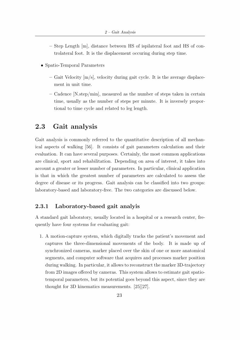
Some examples of optoelectronic systems used in gait analysis are Vicon, Qualisys
Motion Analysis or OptoTrack. In particular, Vicon system provides a clinically
validated solution in any gait analysis or rehabilitation environment, and can be
used to measure or give real-time feedback on the movements of the whole body or
a single part, including hands, face, feet and spine, across different applications, like
stroke rehabilitation, posture analysis, and balance studies. For these reasons, it is
the most commonly and widely choosen (Fig.2.2) [45][53]. To date, analysis with
these systems is widely accepted as ’gold standard’ for gait analysis, because it is
very good in measuring position, and produces well-quantified and accurate results
over short distances. On the other hans, it requires that markers always must be
seen by cameras, therefore needing the right environmental conditions; presents
very long set-up times to position markers adequately, leeding to expensive and
cumbersome equipment attached to the body; and has a limitated workspace for
the patient’s movement, so only a narrow number of consecutive strides can be
measured [23][25][26][27][55].
24
2 – Gait Analysis
Figure 2.2: Example of marker positioning with Vicon system, [45].
2.3.2 Laboratory-free gait analysis
This type of analysis does not require the use of bulky or permanently localized
devices in a laboratory, thus allowing to detect and quantify gait in any place and
at any time. It is carried out using different devices:
1. Inertial measurement unit (IMU), that aggregates different type of MEMS
sensors, such as accelerometers, gyroscopes and magnetometers, individually
or combined. It measures and reports on object’s velocity, acceleration, ori-
entation, and gravitational forces. Accelerometer is the most common type of
inertial sensor, and its ability to measure changes along its sensitive axis makes
it suitable for measuring motion status in human gait; instead gyroscope is an
angular rate sensor that measure the angular velocity of the feet or legs while
walking. IMU can be located on several parts of the body, such as feet, knees,
thighs or waist, individually or combined, so they are weareable system (WS).
The sufficient number of IMU to be used to obtain a relevant and complete
25
2 – Gait Analysis
analysis is under investigation, but certainly the complexity of the measure-
ments is linked to the number of sensors worn by the subject. Moreover, the
miniaturization of IMU allows the possibility of integrating them on instru-
mented insoles for gait analysis. They are ultra-small size, portable, low cost
and pratical useful for longer and natural movements. Furthermore, they do
not require a specific laboratory, but they can be used everywhere, and have
a theorically unlimited workspace. So, IMU can be successfully used for accu-
rate, non-invasive, and ambulatory motion tracking. However, they allow to
estimate temporal and spatial parameters, but the integration of acceleration
signals is subject to drift, leading to measurement errors. In addition, where
the magnetometers are present, they are influenced by the surroundings and
so they limit the settings for the analysis [25][24][26][28][23][55]. However, the
measurements of inertial systems can be compared to optoelectronic systems
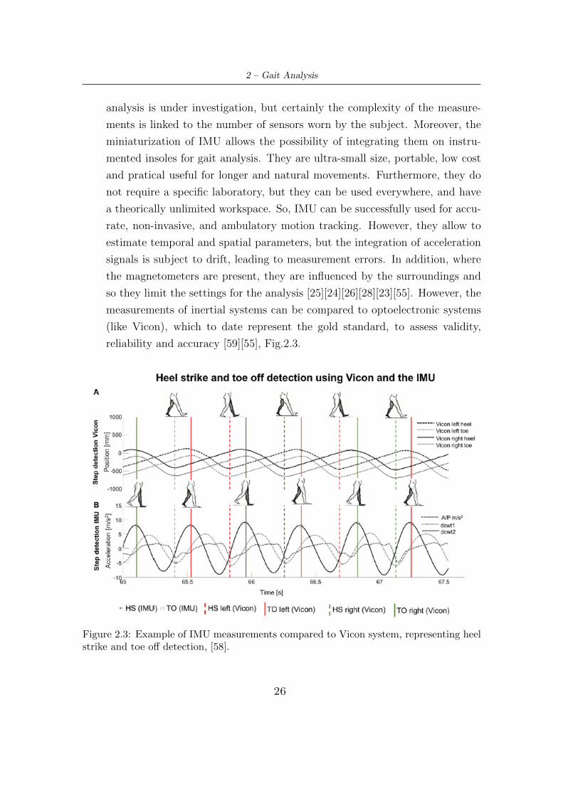
(like Vicon), which to date represent the gold standard, to assess validity,
reliability and accuracy [59][55], Fig.2.3.
Figure 2.3: Example of IMU measurements compared to Vicon system, representing heelstrike and toe off detection, [58].
26
2 – Gait Analysis
2. Smartphone, for the purpose of data collection in daily life. This use is becom-
ing increasingly popular thanks to its easy transport and rich sensing abilities.
It is equipped with accelerometers, gyroscopes and magnetometers that allow
it to be employed in an ever increasing number of fields of application, such as
tracking and positioning, activity recognition, health monitoring, telemedicine
and telerehabilitation. It is a cheaper and user-friendly alternative to IMUs
[49][26][50], which can be used by practically everyone. Indeed, nowadays, any
subject belonging to all age groups has one.
3. Goniometers, ie sensors used to measure the angles of human joints, as an-
klees, knees, hips, ecc. They can be various (strain gauge-based, inductive or
mechanical), and are usually fitted in intrumented shoes to measures ankle to
foot angles [28][24]. Also force-plate sensors can be embedded into footwear
for this type of analysis [25].
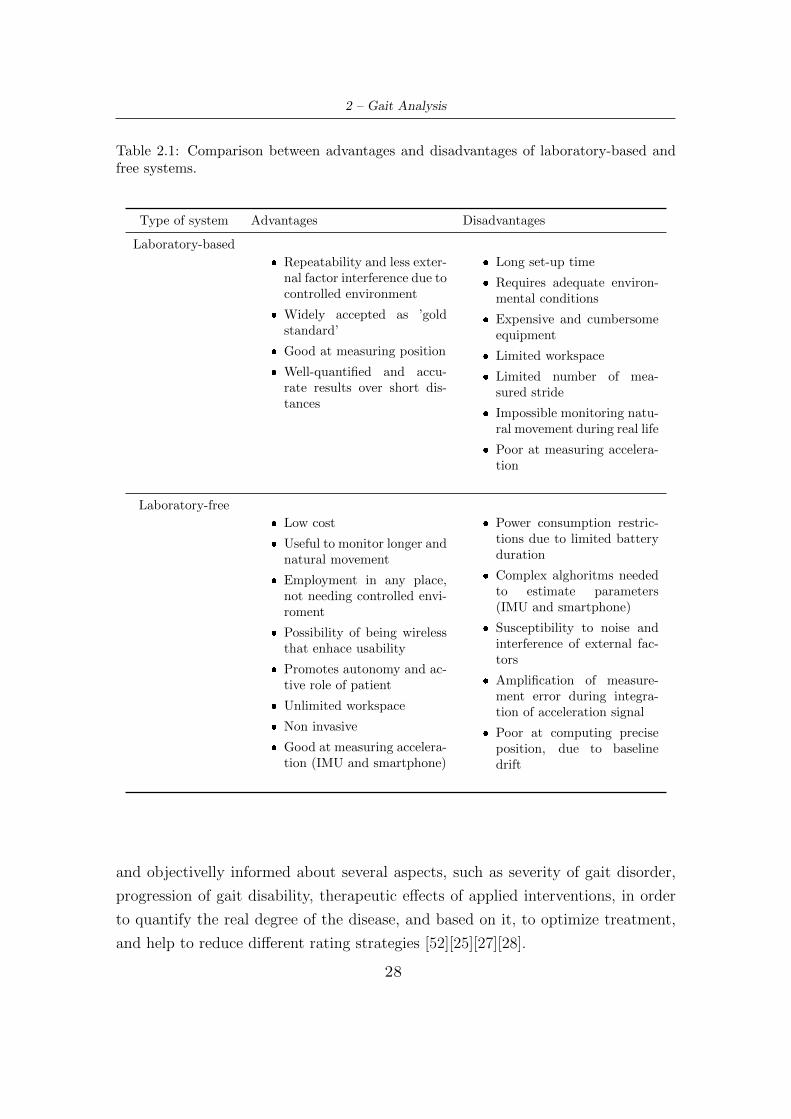
A complete view on the advantages and disadvantages of both categories is shown
in Tab.2.1.
2.4 Gait analysis in Parkinson’s disease
Since it is necessary to evaluate the motor symptoms of PD and their progress
during disease, many clinical assessments have been developed, where the most
common include the Timed up and Go test and the postural instability and gait
disability score derived from the UPDRS. These assessments are easy to accomplish
in clinical setting, because they require little equipment, and also provide imme-
diate outcomes that can be reported to the patient. However, these tests show
poor sensitivity and specificity for identifying prospective fallers in PD population,
and may not be sufficiently sensitive to detect changes in balance and walking in
people who have mild to moderate disease severity, like motor fluctuations, FOG,
falls [52]. This happens because they are subjective and qualitative measurements,
which have a negative effect on the diagnosis, follow-up and treatment of pathology
[23][24][60]. They only offer biased evaluations taken over short periods of time, do
not take into account the long-term patient mobility, but only indicate the condi-
tion at the moment. Moreover, the assessment is dependent on clinician’s expertise
and individual training [27]. So, it would be helpful for clinicians to be reliably
27
2 – Gait Analysis
Table 2.1: Comparison between advantages and disadvantages of laboratory-based andfree systems.
Type of system Advantages Disadvantages
Laboratory-based
� Repeatability and less exter-nal factor interference due tocontrolled environment
� Widely accepted as ’goldstandard’
� Good at measuring position
� Well-quantified and accu-rate results over short dis-tances
� Long set-up time
� Requires adequate environ-mental conditions
� Expensive and cumbersomeequipment
� Limited workspace
� Limited number of mea-sured stride
� Impossible monitoring natu-ral movement during real life
� Poor at measuring accelera-tion
Laboratory-free
� Low cost
� Useful to monitor longer andnatural movement
� Employment in any place,not needing controlled envi-roment
� Possibility of being wirelessthat enhace usability
� Promotes autonomy and ac-tive role of patient
� Unlimited workspace
� Non invasive
� Good at measuring accelera-tion (IMU and smartphone)
� Power consumption restric-tions due to limited batteryduration
� Complex alghoritms neededto estimate parameters(IMU and smartphone)
� Susceptibility to noise andinterference of external fac-tors
� Amplification of measure-ment error during integra-tion of acceleration signal
� Poor at computing preciseposition, due to baselinedrift
and objectivelly informed about several aspects, such as severity of gait disorder,
progression of gait disability, therapeutic effects of applied interventions, in order
to quantify the real degree of the disease, and based on it, to optimize treatment,
and help to reduce different rating strategies [52][25][27][28].
28
2 – Gait Analysis
Therefore, several approaches are utilized to overcome these problems, and to im-
prove the objectivity of measures, in order to track symptoms progression and
evaluate patient risks, resulting in more efficient measurement and providing spe-
cialists with a large amount of reliable information. In particular, gait analysis
allows to detect changes in gait that produce key information about patient’s qual-
ity of life, reducing the error margin caused by subjective techniques [23][24].
A large number of useful gait parameters can be evaluated by both gait categories
previous discussed, to improve the sensitivity, accuracy, reproducibility, and feasi-
bility of measurements about changes in motor behaviours [61][27][28]. Laboratory-
based systems surely represent the gold standard in gait analysis, but considering
the clinical application to Parkinson’s disease, they exhibit several problems. In
fact, a disadvantage is that the monitoring process is carried out in a controlled
enviroment in which the patient feels safe, but many subjects experience the most
severe episodes of impaired gait, FSG and FOG (that present episodic and unpre-
dictable nature) while at home [25]. Moreover, their limited workspace does not
allow the acquisition of a lot information. So, for these reasons, they result partly
inadequate for this application.
Instead, ambulatory gait analysis can provide valuable systems for anywhere-anytime
monitoring of PD individual’s motor behavior [26][49][54]. In fact, this type of anal-
ysis allows to evaluate fluctuating events in response to medication, to capture falls
or FOG episodes, and to assess all physical activities in everyday life, that occur
over long periods and outside the clinical examination room [61][27]. In particular,
a significant number of literature studies supports the use of wearable system, that
have recently shown good reliability for assessing individuals with PD, especially
for acceleration-based measures calculated in the time domain. They are able to
assess standing balance and walking differences for different subgroups of subjects,
like PD fallers and non-fallers, people with PD and controls, people with different
PD subtypes, and also contribute to the diagnosis beetween idiopatich PD and
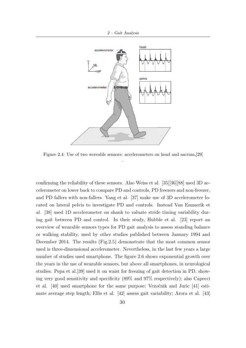
drug-induced parkinsonim [23][26][28]. Latt et al. [29] used two inertial sensors
(accelerometers, Fig.2.4) located in two different body zones (head and sacrum)
to detect and evaluate differences between fallers and non fallers in elderly people
with PD and controls. Their results show significant differences between analyzed
groups (reduced walking speed and step length and increased step time variability),
29
2 – Gait Analysis
Figure 2.4: Use of two wereable sensors: accelerometers on head and sacrum,[29]
.
confirming the reliability of these sensors. Also Weiss et al. [35][36][88] used 3D ac-
celerometer on lower back to compare PD and controls, PD freezers and non-freezer,
and PD fallers with non-fallers. Yang et al. [37] make use of 3D accelerometer lo-
cated on lateral pelvis to investigate PD and controls. Instead Van Emmerik et
al. [38] used 1D accelerometer on shank to valuate stride timing variability dur-
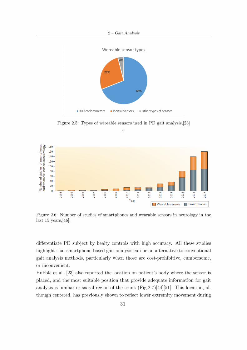
ing gait between PD and control. In their study, Hubble et al. [23] report an
overview of wearable sensors types for PD gait analysis to assess standing balance
or walking stability, used by other studies published between January 1994 and
December 2014. The results (Fig.2.5) demonstrate that the most common sensor
used is three-dimensional accelerometer. Nevertheless, in the last few years a large
number of studies used smartphone. The figure 2.6 shows exponential growth over
the years in the use of wearable sensors, but above all smartphones, in neurological
studies. Pepa et al.[39] used it on waist for freezing of gait detection in PD, show-
ing very good sensitivity and specificity (89% and 97% respectively); also Capecci
et al. [40] used smartphone for the same purpose; Vezocnik and Juric [41] esti-
mate average step length; Ellis et al. [42] assess gait variability; Arora et al. [43]
30
2 – Gait Analysis
Figure 2.5: Types of wereable sensors used in PD gait analysis,[23]
.
Figure 2.6: Number of studies of smartphones and wearable sensors in neurology in thelast 15 years,[46].
differentiate PD subject by healty controls with high accuracy. All these studies
highlight that smartphone-based gait analysis can be an alternative to conventional
gait analysis methods, particularly when those are cost-prohibitive, cumbersome,
or inconvenient.
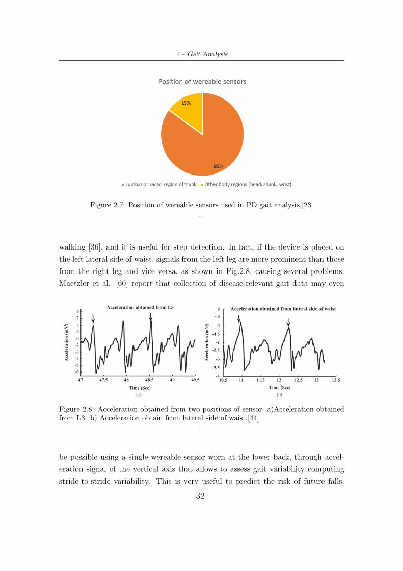
Hubble et al. [23] also reported the location on patient’s body where the sensor is
placed, and the most suitable position that provide adequate information for gait
analysis is lumbar or sacral region of the trunk (Fig.2.7)[44][51]. This location, al-
though centered, has previously shown to reflect lower extremity movement during
31
2 – Gait Analysis
Figure 2.7: Position of wereable sensors used in PD gait analysis,[23]
.
walking [36], and it is useful for step detection. In fact, if the device is placed on
the left lateral side of waist, signals from the left leg are more prominent than those
from the right leg and vice versa, as shown in Fig.2.8, causing several problems.
Maetzler et al. [60] report that collection of disease-relevant gait data may even
Figure 2.8: Acceleration obtained from two positions of sensor- a)Acceleration obtainedfrom L3. b) Acceleration obtain from lateral side of waist,[44]
.
be possible using a single wereable sensor worn at the lower back, through accel-
eration signal of the vertical axis that allows to assess gait variability computing
stride-to-stride variability. This is very useful to predict the risk of future falls.
32
2 – Gait Analysis
Furthermore, always using a sensor at the lower back, differences of anticipatory
postural adjustament between untreated PD patients and control individuals were
found, and this is very important because it is a parameter related to increased
risk of FOG and falling [60]. Also falls, which are sporadic and episodic events that
require long monitoring, balance impairment and mild postural sway abnormalities
can be detected by single sensor with triaxial accelerometer worn at the lower back,
like smartphone [60]. Therefore, the best operational solution for gait analysis in
PD seems to be the use of a 3D accelerometer (as a single inertial sensor or using
the one present in smartphone), positioned at lower waist.
In conclusion, wearable sensors provide a light-weight, portable and affordable al-
ternative to more expensive three-dimensional motion analysis systems and are
effective for detecting changes in standing balance and walking stability among
people with PD [23]. This will enable patients with movement disorders to benefit
from an analysis that has been limited to academic laboratories and state-of-the-art
medical centers [27].
33
Chapter 3
Gait assessment
This chapter describes materials and methods that have been used to extracting and
analyzing measured signals. Different spatio-temporal parameters were calculated
both in PD subjects and in elderly controls. All calculations and signal processing
were performed using Matlab R2018b software.
3.1 Materials
3.1.1 Smartphone sensors characteristics
Before proceeding with the acquisition and elaboration of signals, smartphone sen-
sors characteristics have been evaluated, in particular sampling frequency, range
and resolution, to understand if these were suitable for conducting gait analysis.
� Sensors sample frequency has to respects the Nyquist theorem, according to
which this must be at least twice the maximum useful frequency of the signal
to be acquired. Human activity acceleration signal lie in the 0-20 Hz band
[63], therefore a frequency of at least 40 Hz must be set. Anyhow, the 3-5 Hz
has been defined as ’locomotor band’ [40], and it has also been observed that
normal walking has a principal frequency around 2Hz [62].
� Acceleration signal amplitude range depends on considered direction, location
of sensor and body weight. Considering a waist-mounted sensor, acceleration
amplitude during walking lies in the range ±1g, with g being the gravitational
acceleration.
34
3 – Gait assessment
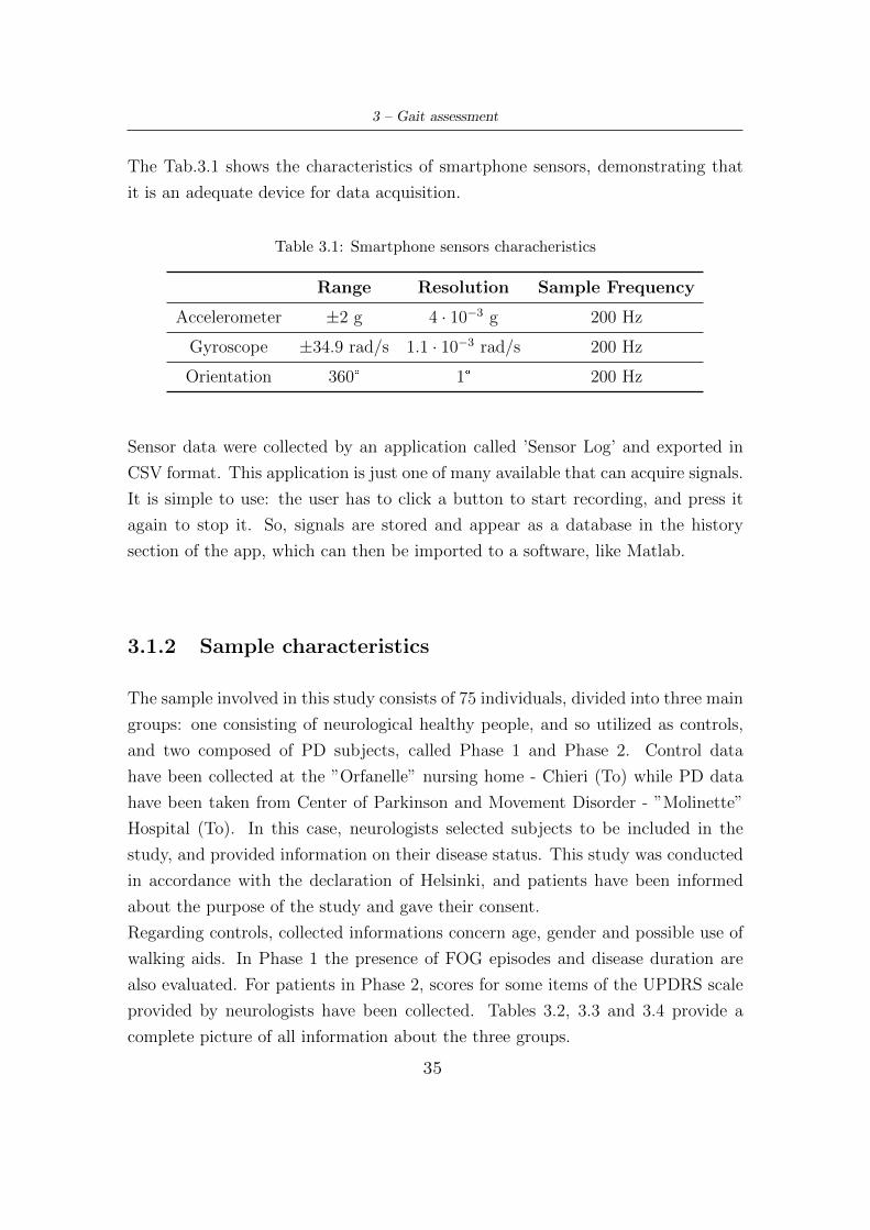
The Tab.3.1 shows the characteristics of smartphone sensors, demonstrating that
it is an adequate device for data acquisition.
Table 3.1: Smartphone sensors characheristics
Range Resolution Sample Frequency
Accelerometer ±2 g 4 · 10−3 g 200 Hz
Gyroscope ±34.9 rad/s 1.1 · 10−3 rad/s 200 Hz
Orientation 360° 1° 200 Hz
Sensor data were collected by an application called ’Sensor Log’ and exported in
CSV format. This application is just one of many available that can acquire signals.
It is simple to use: the user has to click a button to start recording, and press it
again to stop it. So, signals are stored and appear as a database in the history
section of the app, which can then be imported to a software, like Matlab.
3.1.2 Sample characteristics
The sample involved in this study consists of 75 individuals, divided into three main
groups: one consisting of neurological healthy people, and so utilized as controls,
and two composed of PD subjects, called Phase 1 and Phase 2. Control data
have been collected at the ”Orfanelle” nursing home - Chieri (To) while PD data
have been taken from Center of Parkinson and Movement Disorder - ”Molinette”
Hospital (To). In this case, neurologists selected subjects to be included in the
study, and provided information on their disease status. This study was conducted
in accordance with the declaration of Helsinki, and patients have been informed
about the purpose of the study and gave their consent.
Regarding controls, collected informations concern age, gender and possible use of
walking aids. In Phase 1 the presence of FOG episodes and disease duration are
also evaluated. For patients in Phase 2, scores for some items of the UPDRS scale
provided by neurologists have been collected. Tables 3.2, 3.3 and 3.4 provide a
complete picture of all information about the three groups.
35
3 – Gait assessment
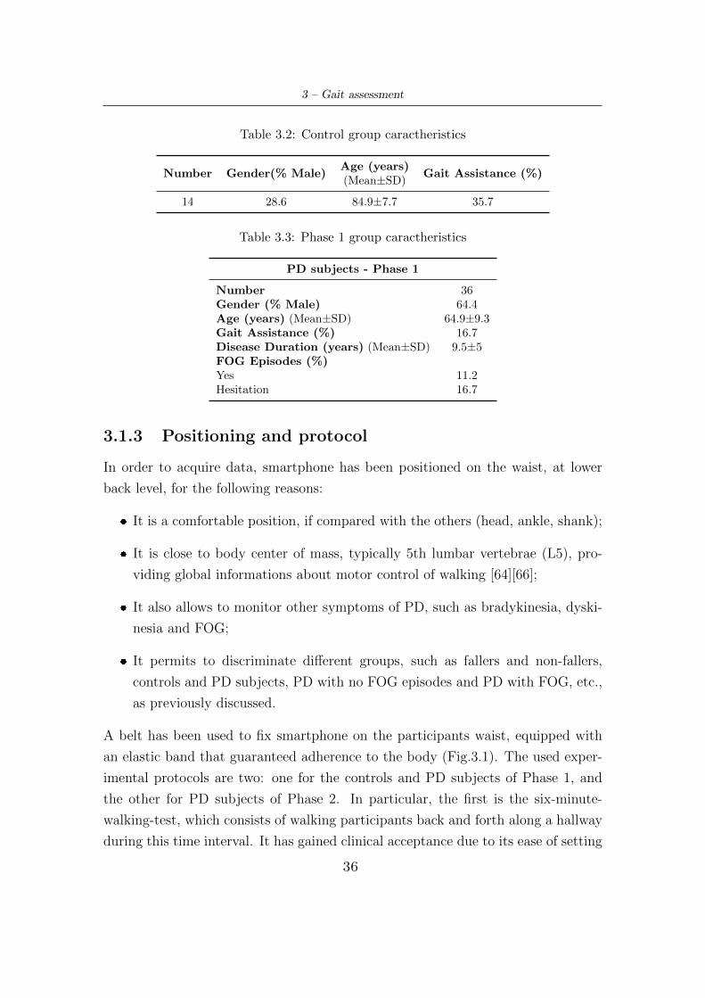
Table 3.2: Control group caractheristics
Number Gender(% Male)Age (years)
Gait Assistance (%)(Mean±SD)
14 28.6 84.9±7.7 35.7
Table 3.3: Phase 1 group caractheristics
PD subjects - Phase 1
Number 36Gender (% Male) 64.4Age (years) (Mean±SD) 64.9±9.3Gait Assistance (%) 16.7Disease Duration (years) (Mean±SD) 9.5±5FOG Episodes (%)Yes 11.2Hesitation 16.7
3.1.3 Positioning and protocol
In order to acquire data, smartphone has been positioned on the waist, at lower
back level, for the following reasons:
� It is a comfortable position, if compared with the others (head, ankle, shank);
� It is close to body center of mass, typically 5th lumbar vertebrae (L5), pro-
viding global informations about motor control of walking [64][66];
� It also allows to monitor other symptoms of PD, such as bradykinesia, dyski-
nesia and FOG;
� It permits to discriminate different groups, such as fallers and non-fallers,
controls and PD subjects, PD with no FOG episodes and PD with FOG, etc.,
as previously discussed.
A belt has been used to fix smartphone on the participants waist, equipped with
an elastic band that guaranteed adherence to the body (Fig.3.1). The used exper-
imental protocols are two: one for the controls and PD subjects of Phase 1, and
the other for PD subjects of Phase 2. In particular, the first is the six-minute-
walking-test, which consists of walking participants back and forth along a hallway
during this time interval. It has gained clinical acceptance due to its ease of setting
36
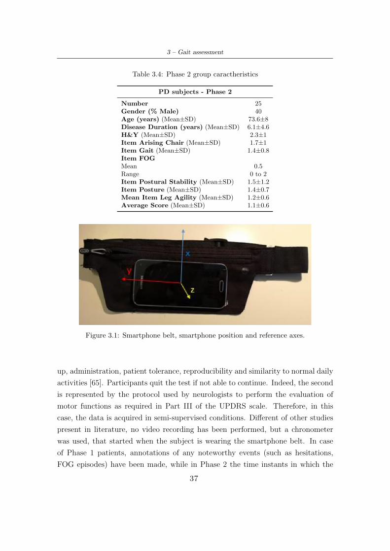
3 – Gait assessment
Table 3.4: Phase 2 group caractheristics
PD subjects - Phase 2
Number 25Gender (% Male) 40Age (years) (Mean±SD) 73.6±8Disease Duration (years) (Mean±SD) 6.1±4.6H&Y (Mean±SD) 2.3±1Item Arising Chair (Mean±SD) 1.7±1Item Gait (Mean±SD) 1.4±0.8Item FOGMean 0.5Range 0 to 2Item Postural Stability (Mean±SD) 1.5±1.2Item Posture (Mean±SD) 1.4±0.7Mean Item Leg Agility (Mean±SD) 1.2±0.6Average Score (Mean±SD) 1.1±0.6
Figure 3.1: Smartphone belt, smartphone position and reference axes.
up, administration, patient tolerance, reproducibility and similarity to normal daily
activities [65]. Participants quit the test if not able to continue. Indeed, the second
is represented by the protocol used by neurologists to perform the evaluation of
motor functions as required in Part III of the UPDRS scale. Therefore, in this
case, the data is acquired in semi-supervised conditions. Different of other studies
present in literature, no video recording has been performed, but a chronometer
was used, that started when the subject is wearing the smartphone belt. In case
of Phase 1 patients, annotations of any noteworthy events (such as hesitations,
FOG episodes) have been made, while in Phase 2 the time instants in which the
37
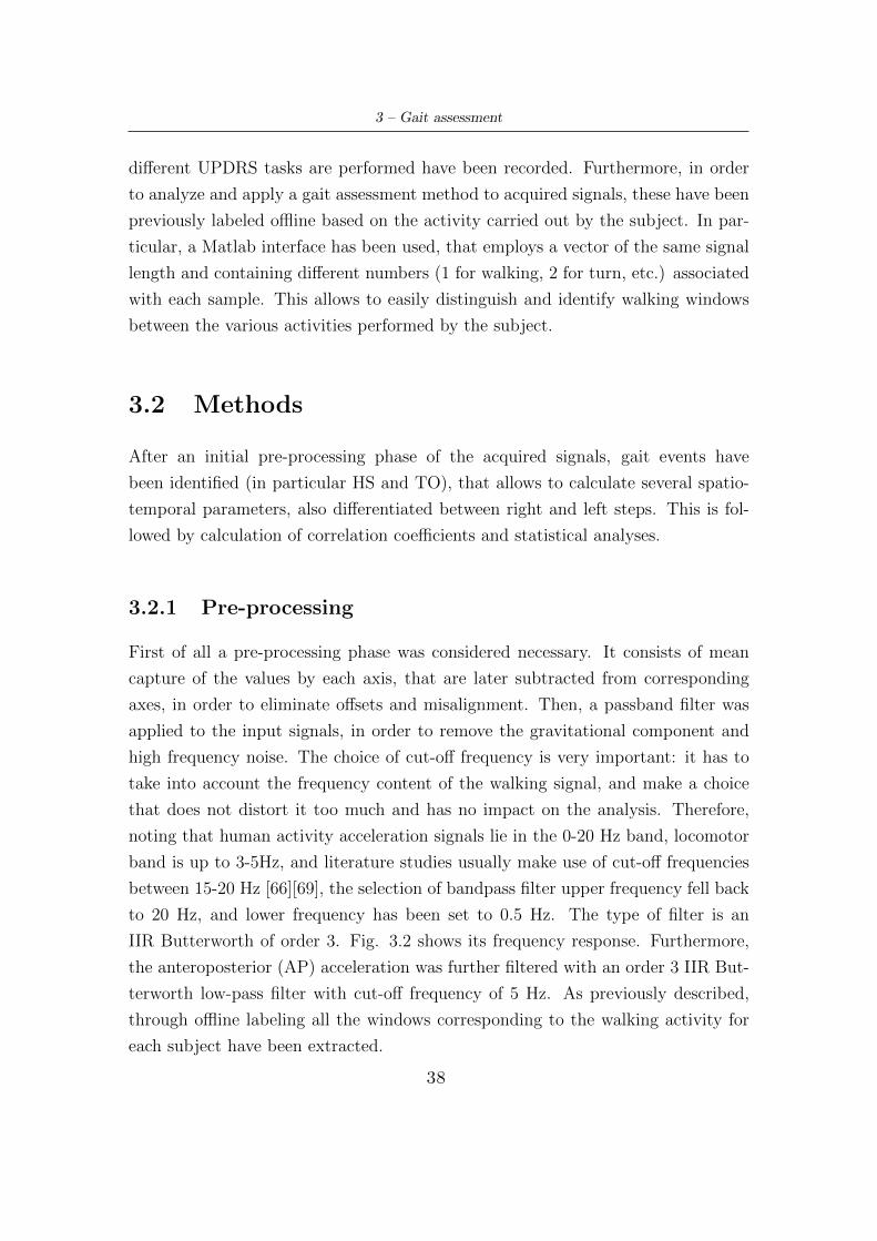
3 – Gait assessment
different UPDRS tasks are performed have been recorded. Furthermore, in order
to analyze and apply a gait assessment method to acquired signals, these have been
previously labeled offline based on the activity carried out by the subject. In par-
ticular, a Matlab interface has been used, that employs a vector of the same signal
length and containing different numbers (1 for walking, 2 for turn, etc.) associated
with each sample. This allows to easily distinguish and identify walking windows
between the various activities performed by the subject.
3.2 Methods
After an initial pre-processing phase of the acquired signals, gait events have
been identified (in particular HS and TO), that allows to calculate several spatio-
temporal parameters, also differentiated between right and left steps. This is fol-
lowed by calculation of correlation coefficients and statistical analyses.
3.2.1 Pre-processing
First of all a pre-processing phase was considered necessary. It consists of mean
capture of the values by each axis, that are later subtracted from corresponding
axes, in order to eliminate offsets and misalignment. Then, a passband filter was
applied to the input signals, in order to remove the gravitational component and
high frequency noise. The choice of cut-off frequency is very important: it has to
take into account the frequency content of the walking signal, and make a choice
that does not distort it too much and has no impact on the analysis. Therefore,
noting that human activity acceleration signals lie in the 0-20 Hz band, locomotor
band is up to 3-5Hz, and literature studies usually make use of cut-off frequencies
between 15-20 Hz [66][69], the selection of bandpass filter upper frequency fell back
to 20 Hz, and lower frequency has been set to 0.5 Hz. The type of filter is an
IIR Butterworth of order 3. Fig. 3.2 shows its frequency response. Furthermore,
the anteroposterior (AP) acceleration was further filtered with an order 3 IIR But-
terworth low-pass filter with cut-off frequency of 5 Hz. As previously described,
through offline labeling all the windows corresponding to the walking activity for
each subject have been extracted.
38
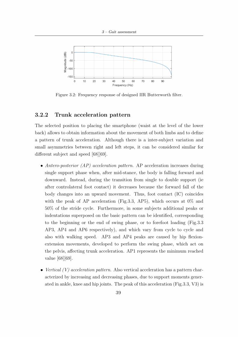
3 – Gait assessment
Figure 3.2: Frequency response of designed IIR Butterworth filter.
3.2.2 Trunk acceleration pattern
The selected position to placing the smartphone (waist at the level of the lower
back) allows to obtain information about the movement of both limbs and to define
a pattern of trunk acceleration. Although there is a inter-subject variation and
small asymmetries between right and left steps, it can be considered similar for
different subject and speed [68][69].
� Antero-posterior (AP) acceleration pattern. AP acceleration increases during
single support phase when, after mid-stance, the body is falling forward and
downward. Instead, during the transition from single to double support (ie
after controlateral foot contact) it decreases because the forward fall of the
body changes into an upward movement. Thus, foot contact (IC) coincides
with the peak of AP acceleration (Fig.3.3, AP5), which occurs at 0% and
50% of the stride cycle. Furthermore, in some subjects additional peaks or
indentations superposed on the basic pattern can be identified, corresponding
to the beginning or the end of swing phase, or to forefoot loading (Fig.3.3
AP3, AP4 and AP6 respectively), and which vary from cycle to cycle and
also with walking speed. AP3 and AP4 peaks are caused by hip flexion-
extension movements, developed to perform the swing phase, which act on
the pelvis, affecting trunk acceleration. AP1 represents the minimum reached
value [68][69].
� Vertical (V) acceleration pattern. Also vertical acceleration has a pattern char-
acterized by increasing and decreasing phases, due to support moments gener-
ated in ankle, knee and hip joints. The peak of this acceleration (Fig.3.3, V3) is
39
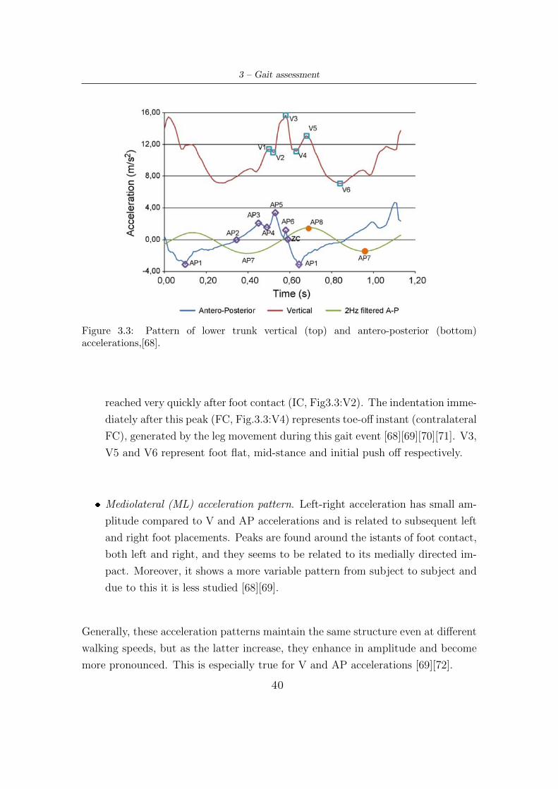
3 – Gait assessment
Figure 3.3: Pattern of lower trunk vertical (top) and antero-posterior (bottom)accelerations,[68].
reached very quickly after foot contact (IC, Fig3.3:V2). The indentation imme-
diately after this peak (FC, Fig.3.3:V4) represents toe-off instant (contralateral
FC), generated by the leg movement during this gait event [68][69][70][71]. V3,
V5 and V6 represent foot flat, mid-stance and initial push off respectively.
� Mediolateral (ML) acceleration pattern. Left-right acceleration has small am-
plitude compared to V and AP accelerations and is related to subsequent left
and right foot placements. Peaks are found around the istants of foot contact,
both left and right, and they seems to be related to its medially directed im-
pact. Moreover, it shows a more variable pattern from subject to subject and
due to this it is less studied [68][69].
Generally, these acceleration patterns maintain the same structure even at different
walking speeds, but as the latter increase, they enhance in amplitude and become
more pronounced. This is especially true for V and AP accelerations [69][72].
40
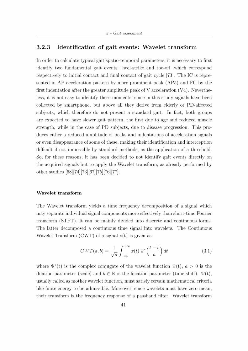
3 – Gait assessment
3.2.3 Identification of gait events: Wavelet transform
In order to calculate typical gait spatio-temporal parameters, it is necessary to first
identify two fundamental gait events: heel-strike and toe-off, which correspond
respectively to initial contact and final contact of gait cycle [73]. The IC is repre-
sented in AP acceleration pattern by more prominent peak (AP5) and FC by the
first indentation after the greater amplitude peak of V acceleration (V4). Neverthe-
less, it is not easy to identify these moments, since in this study signals have been
collected by smartphone, but above all they derive from elderly or PD-affected
subjects, which therefore do not present a standard gait. In fact, both groups
are expected to have slower gait pattern, the first due to age and reduced muscle
strength, while in the case of PD subjects, due to disease progression. This pro-
duces either a reduced amplitude of peaks and indentations of acceleration signals
or even disappearance of some of these, making their identification and interception
difficult if not impossible by standard methods, as the application of a threshold.
So, for these reasons, it has been decided to not identify gait events directly on
the acquired signals but to apply the Wavelet transform, as already performed by
other studies [68][74][73][67][75][76][77].
Wavelet transform
The Wavelet transform yields a time frequency decomposition of a signal which
may separate individual signal components more effectively than short-time Fourier
transform (STFT). It can be mainly divided into discrete and continuous forms.
The latter decomposed a continuous time signal into wavelets. The Continuous
Wavelet Transform (CWT) of a signal x(t) is given as:
CWT (a, b) =1√a
∫ +∞
−∞x(t) Ψ∗
(t− ba
)dt (3.1)
where Ψ∗(t) is the complex conjugate of the wavelet function Ψ(t), a > 0 is the
dilation parameter (scale) and b ∈ R is the location parameter (time shift). Ψ(t),
usually called as mother wavelet function, must satisfy certain mathematical criteria
like finite energy to be admissible. Moreover, since wavelets must have zero mean,
their transform is the frequency response of a passband filter. Wavelet transform
41
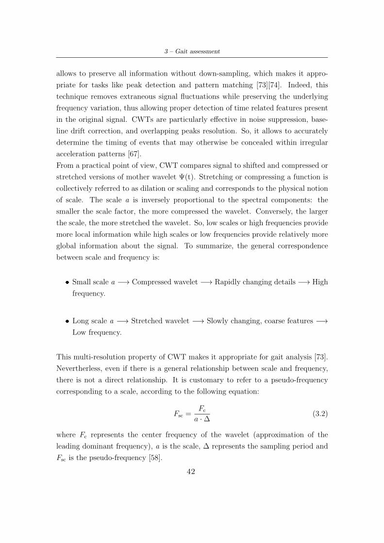
3 – Gait assessment
allows to preserve all information without down-sampling, which makes it appro-
priate for tasks like peak detection and pattern matching [73][74]. Indeed, this
technique removes extraneous signal fluctuations while preserving the underlying
frequency variation, thus allowing proper detection of time related features present
in the original signal. CWTs are particularly effective in noise suppression, base-
line drift correction, and overlapping peaks resolution. So, it allows to accurately
determine the timing of events that may otherwise be concealed within irregular
acceleration patterns [67].
From a practical point of view, CWT compares signal to shifted and compressed or
stretched versions of mother wavelet Ψ(t). Stretching or compressing a function is
collectively referred to as dilation or scaling and corresponds to the physical notion
of scale. The scale a is inversely proportional to the spectral components: the
smaller the scale factor, the more compressed the wavelet. Conversely, the larger
the scale, the more stretched the wavelet. So, low scales or high frequencies provide
more local information while high scales or low frequencies provide relatively more
global information about the signal. To summarize, the general correspondence
between scale and frequency is:
� Small scale a −→ Compressed wavelet −→ Rapidly changing details −→ High
frequency.
� Long scale a −→ Stretched wavelet −→ Slowly changing, coarse features −→Low frequency.
This multi-resolution property of CWT makes it appropriate for gait analysis [73].
Nevertherless, even if there is a general relationship between scale and frequency,
there is not a direct relationship. It is customary to refer to a pseudo-frequency
corresponding to a scale, according to the following equation:
Fsc =Fc
a ·∆(3.2)
where Fc represents the center frequency of the wavelet (approximation of the
leading dominant frequency), a is the scale, ∆ represents the sampling period and
Fsc is the pseudo-frequency [58].
42
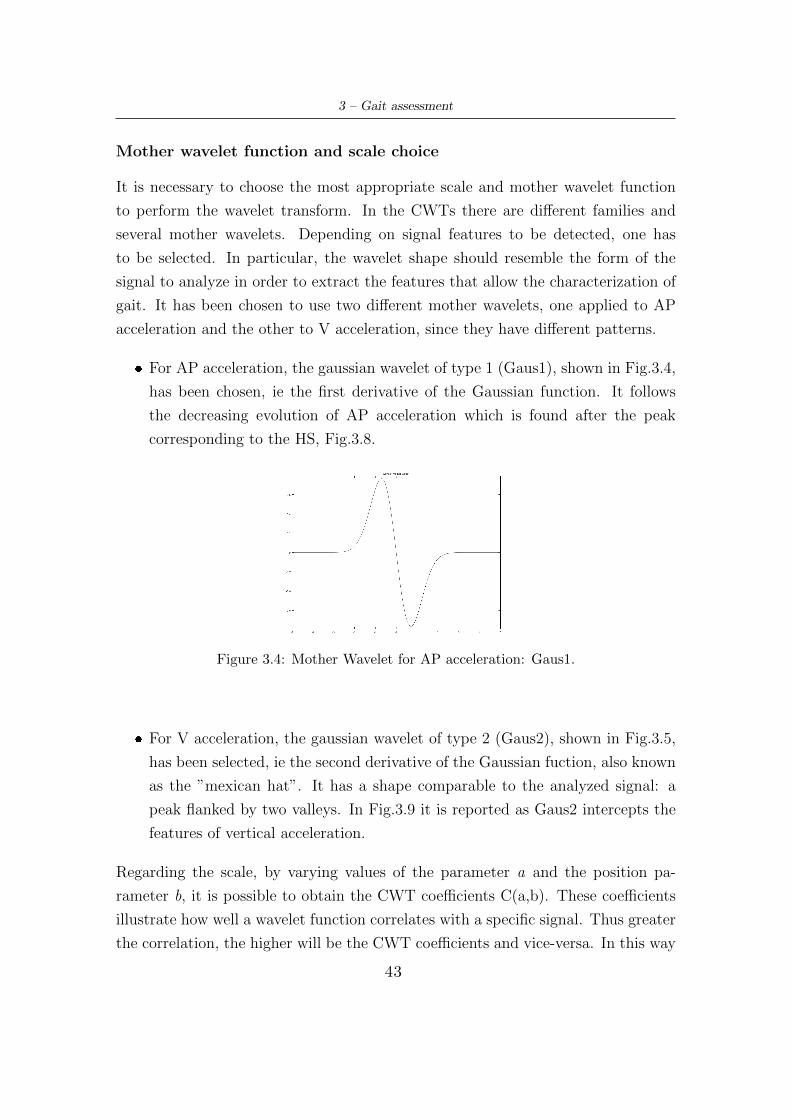
3 – Gait assessment
Mother wavelet function and scale choice
It is necessary to choose the most appropriate scale and mother wavelet function
to perform the wavelet transform. In the CWTs there are different families and
several mother wavelets. Depending on signal features to be detected, one has
to be selected. In particular, the wavelet shape should resemble the form of the
signal to analyze in order to extract the features that allow the characterization of
gait. It has been chosen to use two different mother wavelets, one applied to AP
acceleration and the other to V acceleration, since they have different patterns.
� For AP acceleration, the gaussian wavelet of type 1 (Gaus1), shown in Fig.3.4,
has been chosen, ie the first derivative of the Gaussian function. It follows
the decreasing evolution of AP acceleration which is found after the peak
corresponding to the HS, Fig.3.8.
Figure 3.4: Mother Wavelet for AP acceleration: Gaus1.
� For V acceleration, the gaussian wavelet of type 2 (Gaus2), shown in Fig.3.5,
has been selected, ie the second derivative of the Gaussian fuction, also known
as the ”mexican hat”. It has a shape comparable to the analyzed signal: a
peak flanked by two valleys. In Fig.3.9 it is reported as Gaus2 intercepts the
features of vertical acceleration.
Regarding the scale, by varying values of the parameter a and the position pa-
rameter b, it is possible to obtain the CWT coefficients C(a,b). These coefficients
illustrate how well a wavelet function correlates with a specific signal. Thus greater
the correlation, the higher will be the CWT coefficients and vice-versa. In this way
43
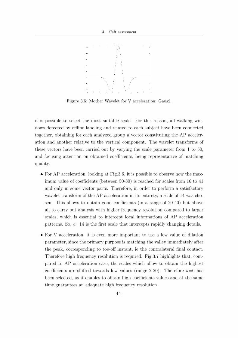
3 – Gait assessment
Figure 3.5: Mother Wavelet for V acceleration: Gaus2.
it is possible to select the most suitable scale. For this reason, all walking win-
dows detected by offline labeling and related to each subject have been connected
together, obtaining for each analyzed group a vector constituting the AP acceler-
ation and another relative to the vertical component. The wavelet transforms of
these vectors have been carried out by varying the scale parameter from 1 to 50,
and focusing attention on obtained coefficients, being representative of matching
quality.
� For AP acceleration, looking at Fig.3.6, it is possible to observe how the max-
imum value of coefficients (between 50-80) is reached for scales from 16 to 41
and only in some vector parts. Therefore, in order to perform a satisfactory
wavelet transform of the AP acceleration in its entirety, a scale of 14 was cho-
sen. This allows to obtain good coefficients (in a range of 20-40) but above
all to carry out analysis with higher frequency resolution compared to larger
scales, which is essential to intercept local informations of AP acceleration
patterns. So, a=14 is the first scale that intercepts rapidly changing details.
� For V acceleration, it is even more important to use a low value of dilation
parameter, since the primary purpose is matching the valley immediately after
the peak, corresponding to toe-off instant, ie the contralateral final contact.
Therefore high frequency resolution is required. Fig.3.7 highlights that, com-
pared to AP acceleration case, the scales which allow to obtain the highest
coefficients are shifted towards low values (range 2-20). Therefore a=6 has
been selected, as it enables to obtain high coefficients values and at the same
time guarantees an adequate high frequency resolution.
44
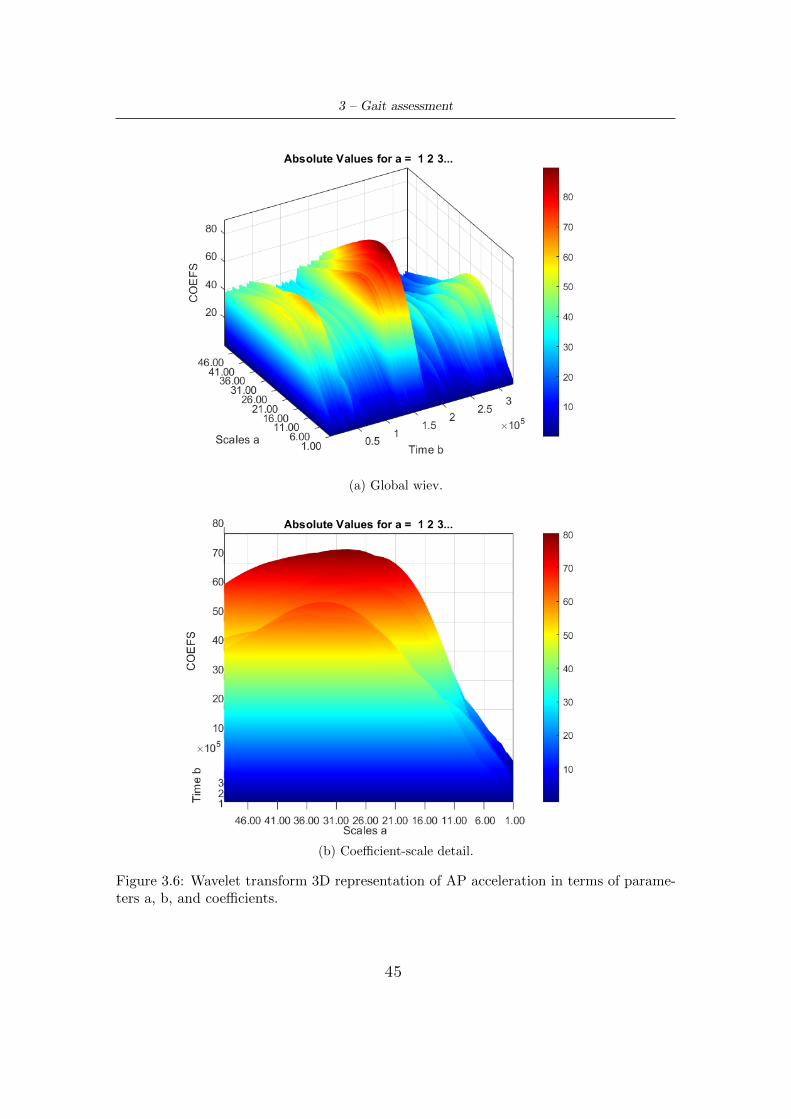
3 – Gait assessment
(a) Global wiev.
(b) Coefficient-scale detail.
Figure 3.6: Wavelet transform 3D representation of AP acceleration in terms of parame-ters a, b, and coefficients.
45
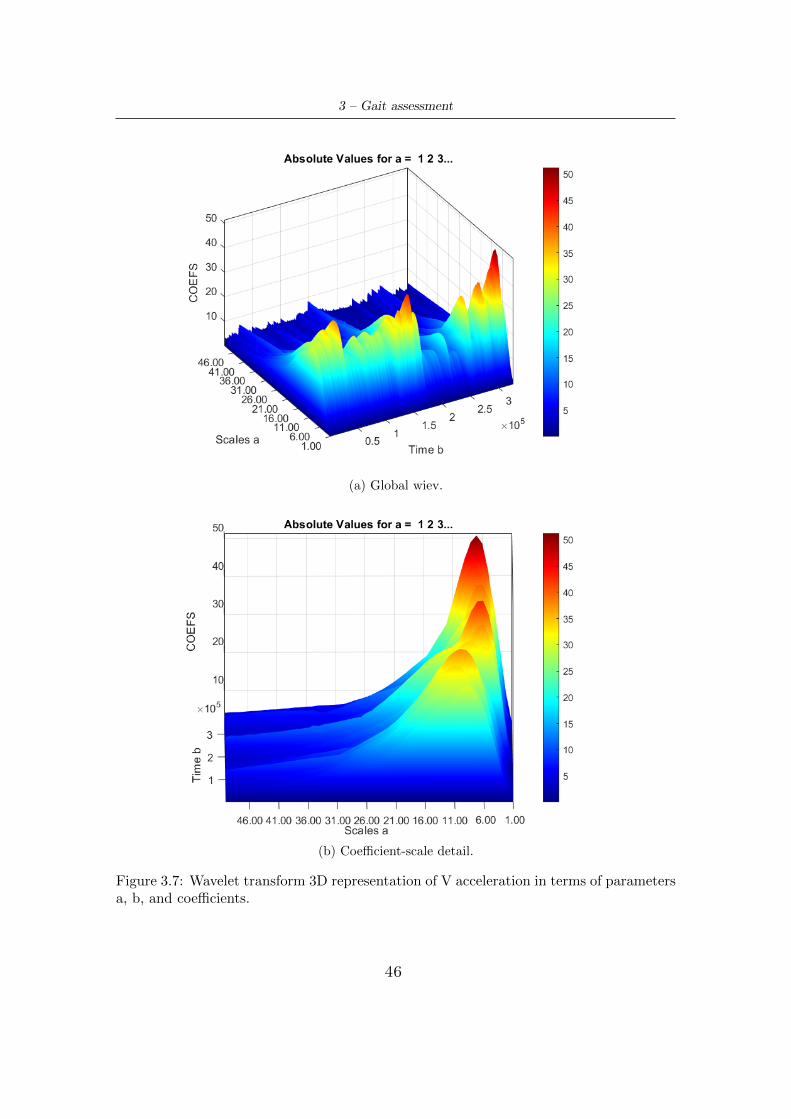
3 – Gait assessment
(a) Global wiev.
(b) Coefficient-scale detail.
Figure 3.7: Wavelet transform 3D representation of V acceleration in terms of parametersa, b, and coefficients.
46
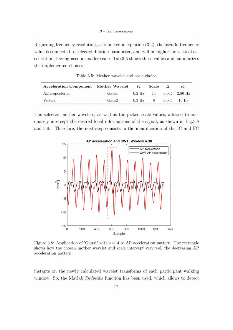
3 – Gait assessment
Regarding frequency resolution, as reported in equation (3.2), the pseudo-frequency
value is connected to selected dilation parameter, and will be higher for vertical ac-
celeration, having used a smaller scale. Tab.3.5 shows these values and summarizes
the implemented choices.
Table 3.5: Mother wavelet and scale choice.
Acceleration Component Mother Wavelet Fc Scale ∆ Fsc
Anteroposterior Gaus1 0.2 Hz 14 0.005 2.86 Hz
Vertical Gaus2 0.3 Hz 6 0.005 10 Hz
The selected mother wavelets, as well as the picked scale values, allowed to ade-
quately intercept the desired local informations of the signal, as shown in Fig.3.8
and 3.9. Therefore, the next step consists in the identification of the IC and FC
Figure 3.8: Application of ’Gaus1’ with a=14 to AP acceleration pattern. The rectangleshows how the chosen mother wavelet and scale intercept very well the decreasing APacceleration pattern.
instants on the newly calculated wavelet transforms of each participant walking
window. So, the Matlab findpeaks function has been used, which allows to detect
47
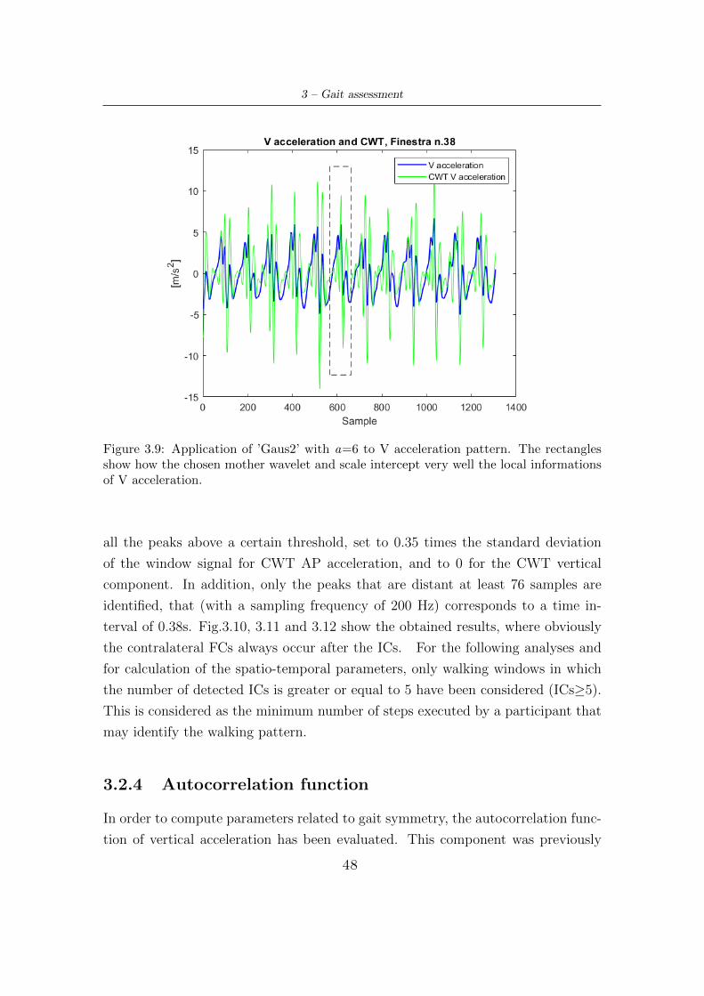
3 – Gait assessment
Figure 3.9: Application of ’Gaus2’ with a=6 to V acceleration pattern. The rectanglesshow how the chosen mother wavelet and scale intercept very well the local informationsof V acceleration.
all the peaks above a certain threshold, set to 0.35 times the standard deviation
of the window signal for CWT AP acceleration, and to 0 for the CWT vertical
component. In addition, only the peaks that are distant at least 76 samples are
identified, that (with a sampling frequency of 200 Hz) corresponds to a time in-
terval of 0.38s. Fig.3.10, 3.11 and 3.12 show the obtained results, where obviously
the contralateral FCs always occur after the ICs. For the following analyses and
for calculation of the spatio-temporal parameters, only walking windows in which
the number of detected ICs is greater or equal to 5 have been considered (ICs≥5).
This is considered as the minimum number of steps executed by a participant that
may identify the walking pattern.
3.2.4 Autocorrelation function
In order to compute parameters related to gait symmetry, the autocorrelation func-
tion of vertical acceleration has been evaluated. This component was previously
48
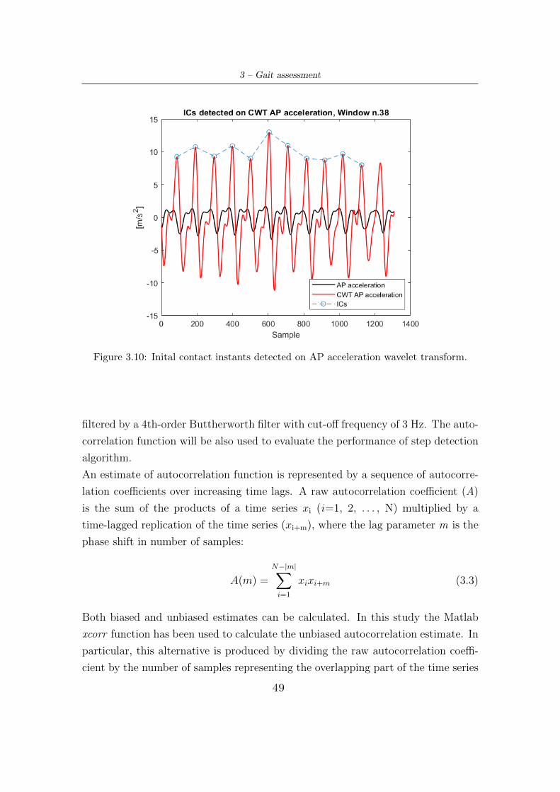
3 – Gait assessment
Figure 3.10: Inital contact instants detected on AP acceleration wavelet transform.
filtered by a 4th-order Buttherworth filter with cut-off frequency of 3 Hz. The auto-
correlation function will be also used to evaluate the performance of step detection
algorithm.
An estimate of autocorrelation function is represented by a sequence of autocorre-
lation coefficients over increasing time lags. A raw autocorrelation coefficient (A)
is the sum of the products of a time series xi (i=1, 2, . . . , N) multiplied by a
time-lagged replication of the time series (xi+m), where the lag parameter m is the
phase shift in number of samples:
A(m) =
N−|m|∑i=1
xixi+m (3.3)
Both biased and unbiased estimates can be calculated. In this study the Matlab
xcorr function has been used to calculate the unbiased autocorrelation estimate. In
particular, this alternative is produced by dividing the raw autocorrelation coeffi-
cient by the number of samples representing the overlapping part of the time series
49
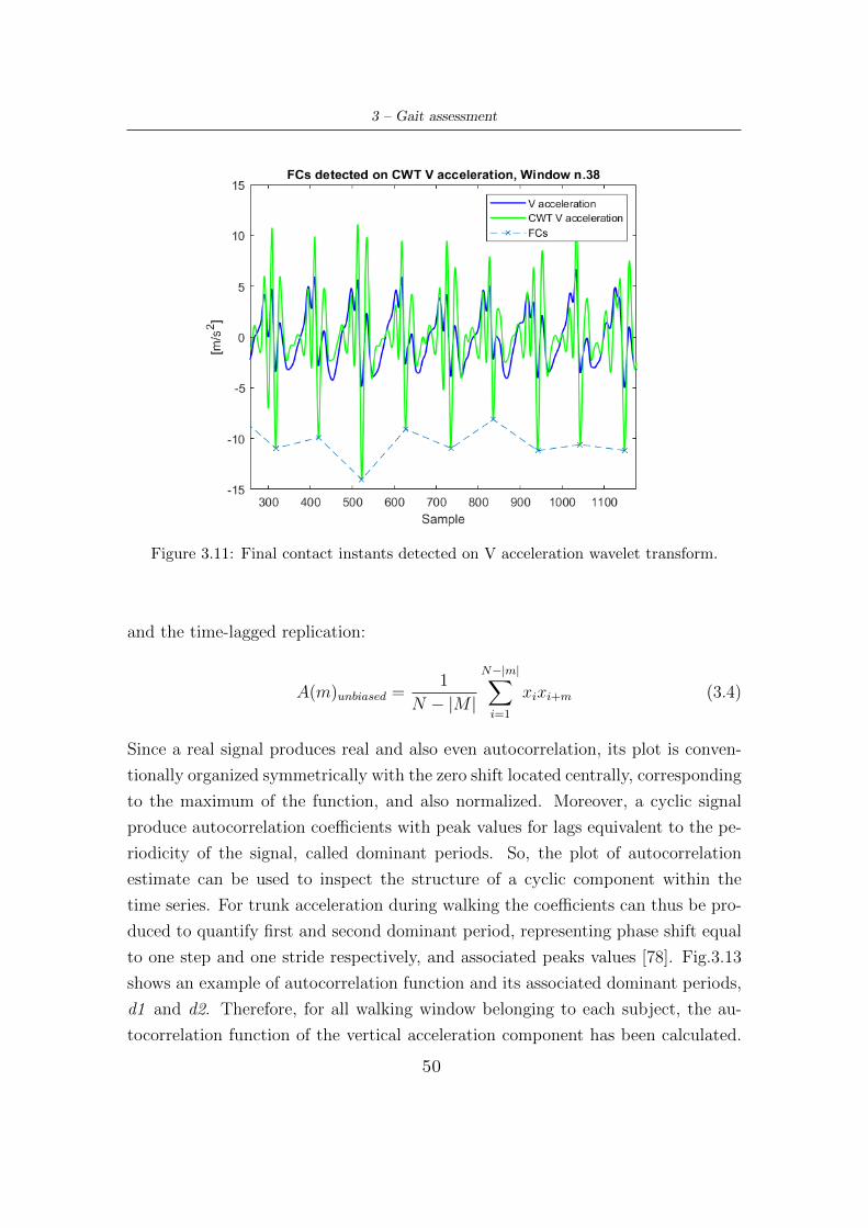
3 – Gait assessment
Figure 3.11: Final contact instants detected on V acceleration wavelet transform.
and the time-lagged replication:
A(m)unbiased =1
N − |M |
N−|m|∑i=1
xixi+m (3.4)
Since a real signal produces real and also even autocorrelation, its plot is conven-
tionally organized symmetrically with the zero shift located centrally, corresponding
to the maximum of the function, and also normalized. Moreover, a cyclic signal
produce autocorrelation coefficients with peak values for lags equivalent to the pe-
riodicity of the signal, called dominant periods. So, the plot of autocorrelation
estimate can be used to inspect the structure of a cyclic component within the
time series. For trunk acceleration during walking the coefficients can thus be pro-
duced to quantify first and second dominant period, representing phase shift equal
to one step and one stride respectively, and associated peaks values [78]. Fig.3.13
shows an example of autocorrelation function and its associated dominant periods,
d1 and d2. Therefore, for all walking window belonging to each subject, the au-
tocorrelation function of the vertical acceleration component has been calculated.
50
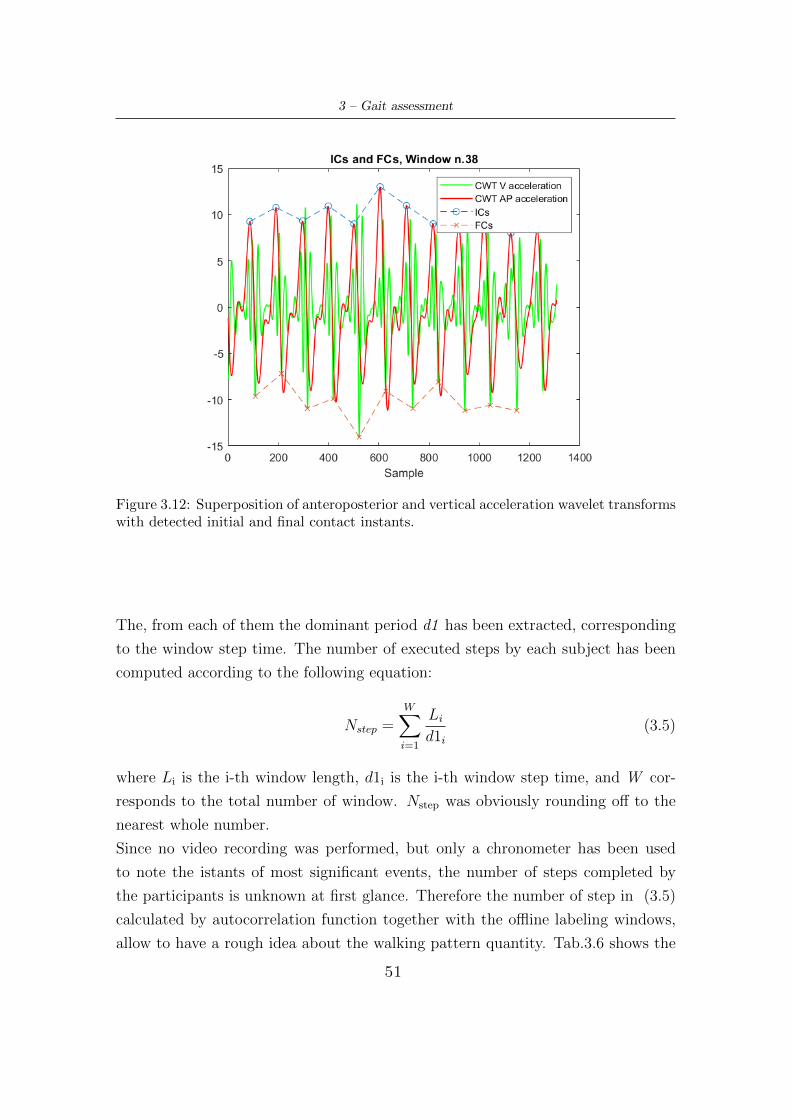
3 – Gait assessment
Figure 3.12: Superposition of anteroposterior and vertical acceleration wavelet transformswith detected initial and final contact instants.
The, from each of them the dominant period d1 has been extracted, corresponding
to the window step time. The number of executed steps by each subject has been
computed according to the following equation:
Nstep =W∑i=1
Li
d1i
(3.5)
where Li is the i-th window length, d1i is the i-th window step time, and W cor-
responds to the total number of window. Nstep was obviously rounding off to the
nearest whole number.
Since no video recording was performed, but only a chronometer has been used
to note the istants of most significant events, the number of steps completed by
the participants is unknown at first glance. Therefore the number of step in (3.5)
calculated by autocorrelation function together with the offline labeling windows,
allow to have a rough idea about the walking pattern quantity. Tab.3.6 shows the
51
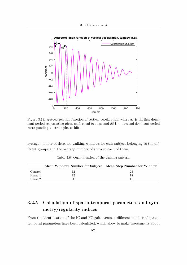
3 – Gait assessment
Figure 3.13: Autocorrelation function of vertical acceleration, where d1 is the first domi-nant period representing phase shift equal to steps and d2 is the second dominant periodcorresponding to stride phase shift.
average number of detected walking windows for each subject belonging to the dif-
ferent groups and the average number of steps in each of them.
Table 3.6: Quantification of the walking pattern.
Mean Windows Number for Subject Mean Step Number for Window
Control 12 23Phase 1 12 18Phase 2 4 11
3.2.5 Calculation of spatio-temporal parameters and sym-
metry/regularity indices
From the identification of the IC and FC gait events, a different number of spatio-
temporal parameters have been calculated, which allow to make assessments about
52
3 – Gait assessment
the quality of walking in the different groups of participants. They are computed
as Mean±SD (Standard Deviation) for each walking window and then mediated for
each subject. These are:
� Cadence [N.step/min]:
Cadence =NICs · 60
Li
fs
(3.6)
where NICs is the number of ICs in a window, Li the i-th window length and
fs the sampling frequency.
� Stride Time [s], as the time interval between two non-consecutive ICs (belong-
ing to the same foot), representative of the gait cycle:
StrideT ime = ICj+2 − ICj (3.7)
� Step Time [s], as the time interval between two consecutive ICs (belonging to
different foot):
StepT ime = ICj+1 − ICj (3.8)
� Swing Time [s], as the difference between IC and the previous FC:
SwingT ime = ICj+1 − FCj (3.9)
� Swing Phase [%GC], swing expressed as percentage of gait cycle.
� Stance Time [s], as the difference between FC and the previous IC:
StanceT ime = FCj+1 − ICj (3.10)
� Stance Phase [%GC], stance expressed as percentage of gait cycle.
� Single Support Time [s], as:
SingleSupportT ime = (ICj − FCj−1) + (ICj+1 − FCj) (3.11)
� Single Support Phase [%GC], expressed as percentage of gait cycle.
53
3 – Gait assessment
� Double Support Time [s], as:
DoubleSupportT ime = (FCj − ICj) + (FCj−1 − ICj−1) (3.12)
� Double Support Phase [%GC], expressed as percentage of gait cycle.
� Step Length [m], estimated using the upward and downward movements of
the trunk. Zijlstra et al. [79] have demonstrated that three-dimensional dis-
placements of the lower trunk during walking are well predicted by an inverted
pendulum model of the body’s centre of mass (COM) trajectory. Assuming
a compass gait type, COM movements in the sagittal plane follow a circular
trajectory during each single support phase. In this model, changes in height
of COM depend on step length. Thus, when changes in height are known, this
parameter can be predicted from geometrical characteristics as:
StepLength = 2 ·√
2lhj − h2j (3.13)
where hj is equal to the change in height of the COM, and l is pendulum length.
Changes in vertical position have been calculated by a double integration of
vertical acceleration through cumtrapz function and then detrend function to
remove integration drift. The amplitude of changes in vertical position (hj) has
been determined as the difference between highest and lowest position during
a step cycle. Instead, the pendulum lenght l is represented by leg length. Since
this value for each subject has not been annotated, a unique value has been
selected for all participants that could be representative for both women and
men. This is 0.85 m. So, from these data, step length has been estimated [69].
� Gait Velocity [m/s], computed as the ratio between step length and step time:
GaitV elocity =StepLengthjStepT imej
(3.14)
� The variation coefficient (CV) has been also calculated for some of the param-
eters just described, as:
CV =SDparameter
Meanparameter
· 100 (3.15)
54
3 – Gait assessment
since it is another way to express the variability of a parameter.
Some of these parameters are reported in Fig.3.14. Moreover the algorithm removes
the parameters value of stride time, swing and stance (and subsequently of double
and single support) not belonging to specific ranges:
1. The average stride time is considered to be around 1.03s, but in particular
cases it can decrease to 0.67s (for young subject)[81], or significantly increase
due to a very slow pattern, reaching values close to 1.18s [35]. So it has been
chosen to remove stride time values lower than 0.7 s, as this study does not
include young subjects, but only elderly controls and PD partecipants.
2. Regarding swing, PD subjects may not have physiological values but lower
ones, even around 33% of GC. To maintain a certain security level due to
inter-subject variability, it has been decided to remove swing values lower
than 29.5%. As for the upper limit, 45.5% has been set, because excessive
swing values (and consequently too small stance values) are only typical at
high walking speeds, and this is not the considered case [47].
3. About stance, the discussion is reciprocal to the swing, so the lower limit has
been set at 55.5% and the upper limit at 70.5%.
Moreover, symmetry/regularity indices have also been calculated in addition to
spatio-temporal parameters. In particular these were obtained from the previously
implemented autocorrelation function [78], as shown in Fig.3.15. They are:
� Step Regularity Ad1 : it is the autocorrelation coefficient corresponding to the
first dominant period d1 that represents a phase shift of one step. So, it is an
expression of the regularity of vertical acceleration signal between neighboring
steps. It ranges between 0 and 1: if it assumes low values, this demonstrates
low regularity between steps; on the contrary values around 1 indicate more
rythimc, consistent and stable walking pattern.
� Stride regularity Ad2 : it is the autocorrelation coefficient corresponding to the
second dominant period d2 that represents a phase shift of one stride. So, it
is a measure of the regularity between neighboring strides. As well as Ad1, it
ranges between 0 and 1, with the same meaning.
55
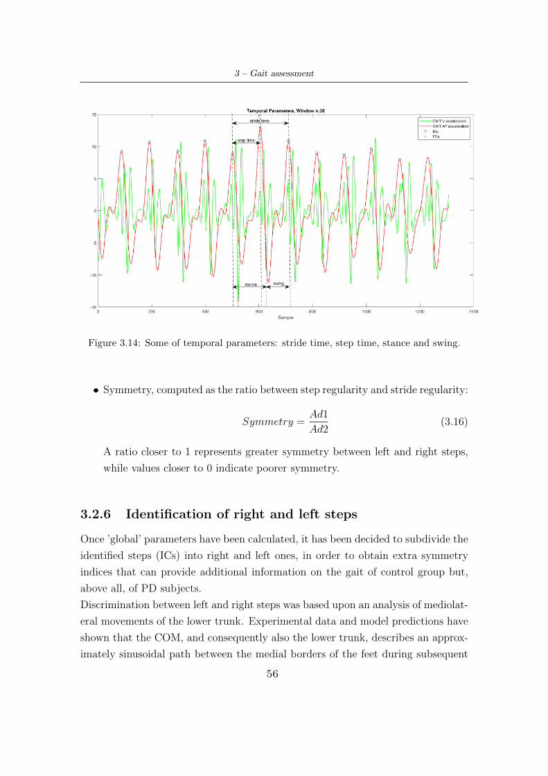
3 – Gait assessment
Figure 3.14: Some of temporal parameters: stride time, step time, stance and swing.
� Symmetry, computed as the ratio between step regularity and stride regularity:
Symmetry =Ad1
Ad2(3.16)
A ratio closer to 1 represents greater symmetry between left and right steps,
while values closer to 0 indicate poorer symmetry.
3.2.6 Identification of right and left steps
Once ’global’ parameters have been calculated, it has been decided to subdivide the
identified steps (ICs) into right and left ones, in order to obtain extra symmetry
indices that can provide additional information on the gait of control group but,
above all, of PD subjects.
Discrimination between left and right steps was based upon an analysis of mediolat-
eral movements of the lower trunk. Experimental data and model predictions have
shown that the COM, and consequently also the lower trunk, describes an approx-
imately sinusoidal path between the medial borders of the feet during subsequent
56
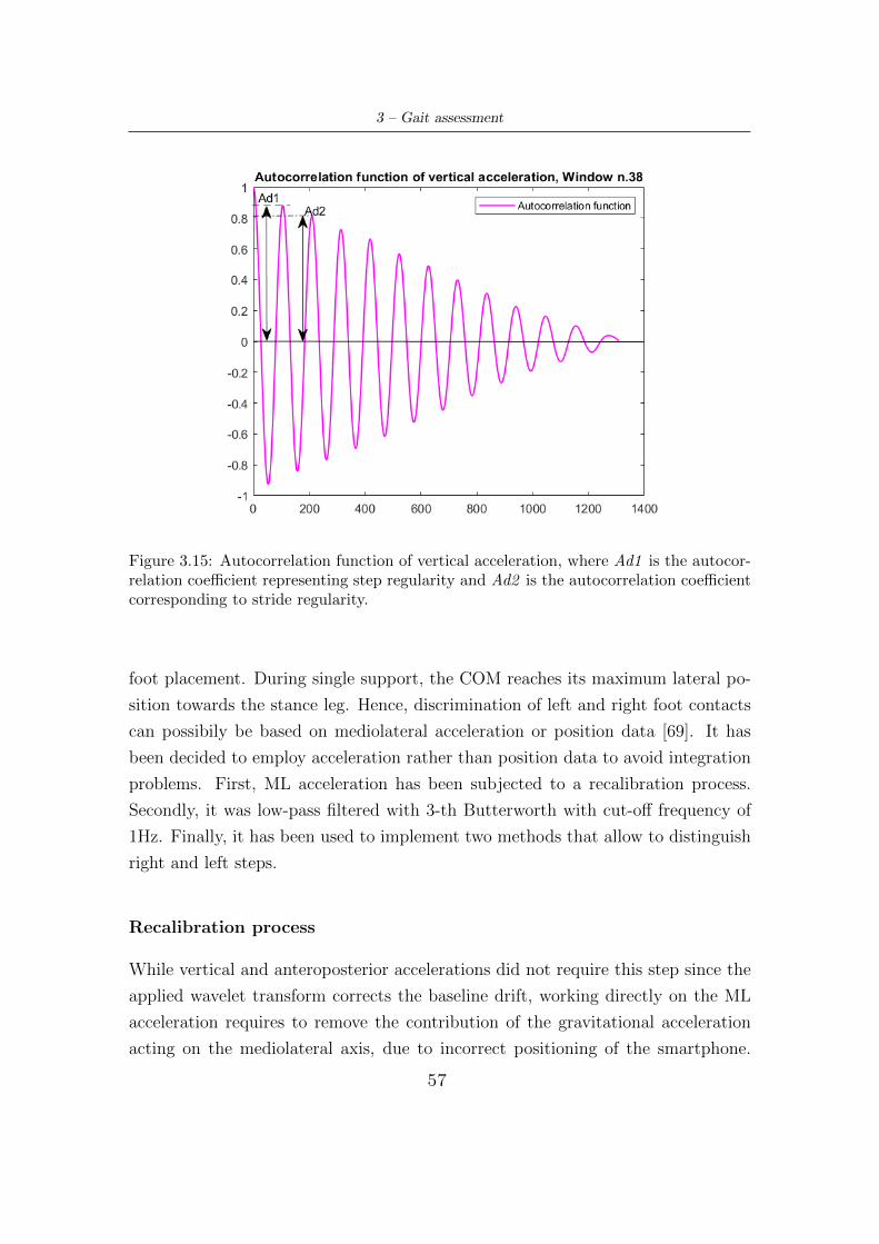
3 – Gait assessment
Figure 3.15: Autocorrelation function of vertical acceleration, where Ad1 is the autocor-relation coefficient representing step regularity and Ad2 is the autocorrelation coefficientcorresponding to stride regularity.
foot placement. During single support, the COM reaches its maximum lateral po-
sition towards the stance leg. Hence, discrimination of left and right foot contacts
can possibily be based on mediolateral acceleration or position data [69]. It has
been decided to employ acceleration rather than position data to avoid integration
problems. First, ML acceleration has been subjected to a recalibration process.
Secondly, it was low-pass filtered with 3-th Butterworth with cut-off frequency of
1Hz. Finally, it has been used to implement two methods that allow to distinguish
right and left steps.
Recalibration process
While vertical and anteroposterior accelerations did not require this step since the
applied wavelet transform corrects the baseline drift, working directly on the ML
acceleration requires to remove the contribution of the gravitational acceleration
acting on the mediolateral axis, due to incorrect positioning of the smartphone.
57
3 – Gait assessment
A common source of error with a waist-mounted smartphone is the resting device
angle due to waist girth, clothing, or the device’s holster [80]. The recalibration
method corrects accelerometer axis orientation by applying a quaternion rotation
transformation to the device’s raw data. It involves constructing the quaternion
rotation matrix by way of the axis-angle representation. A rotation matrix describes
a coordinate system orientation with respect to another orientation. A vector ~V in
the initial reference frame F can be transformed into a vector ~V ’ in a rotated frame
F’ by multiplication of ~V with the rotation matrix between F and F’. Rotation
matrices are orthogonal, square and invertible:
RT = R−1, detR = 1. (3.17)
First, the axis vector is produced by taking the cross product of the initial orien-
tation gravitational vector with the desired orientation gravitational vector. Then,
the dot product is used to solve for the rotation angle α, which is then used with
axis vector as input to build the quaternion rotation matrix. Finally, all raw ac-
celerometer data thereafter are multipilied by the rotation matrix to achieve the
corrected orientation. It is desired to have the gravitational component application
only along the vertical axis, ie in X direction. The initial vector ~Vi contains the
mean acceleration values along the three axes, obtained from the walking window
which for each subject had the greatest length:
~Vi = Xi+ Y j + Zk (3.18)
Instead, the final vector ~Vf is:
~Vf = X ′i+ Y ′j + Z ′k = [−9.81, 0, 0] (3.19)
Considering the initial vector ~Vi and the desired vector ~Vf , it is possible to express
the following equation:~Vf = R~Vi (3.20)
58
3 – Gait assessment
To construct the set of quaternions that yield the required rotation, it is necessary
to first produce an axis-angle pair. The axis vector ~A can be found from the cross-
product bewteen ~Vi and ~Vf :
~A = ~Vi × ~Vf = (9.81Z)j + (−9.81Y )k (3.21)
The axis vector ~A from (3.21) can then be normalized by dividing the magnitude
of ~A:~Anorm =
(Z√
Y 2 + Z2
)j −
(Y√
Y 2 + Z2
)k (3.22)
The angle between vectors can be expressed as the cosine from the dot product.
Using initial vector ~Vi and vector ~Vf we obtain:
~Vi · ~Vf = ‖~Vi‖‖~Vf‖ cos(α) = XX ′ + Y Y ′ + ZZ ′ (3.23)
Since Y’ and Z’=0, and the magnitude of ~Vf equals X’, the equation becomes:
α = arccos
(X
‖~Vi‖
)(3.24)
Therefore, since the axis-angle pair was obtained, it can be use to build the quater-
nion rotation matrix as:
R(q0, q1, q2, q3) =
1− 2(q22 + q23) 2(q1q2 − q0q3) 2(q0q2 + q1q3)
2(q1q2 + q0q3) 1− 2(q21 + q23) 2(q2q3 − q0q1)2(q1q3 − q0q2) 2(q0q1 + q2q3) 1− 2(q21 + q22)
(3.25)
where q0,q1,q2,q3 are:
q0 = cos(α/2) (3.26a)
q1 = sin(α/2)Anorm,x′ (3.26b)
q2 = sin(α/2)Anorm,y′ (3.26c)
q3 = sin(α/2)Anorm,z′ (3.26d)
So, multiplying the raw acceleration by the rotation matrix in equation (3.25), the
revision of orientation has been obtained [80].
59
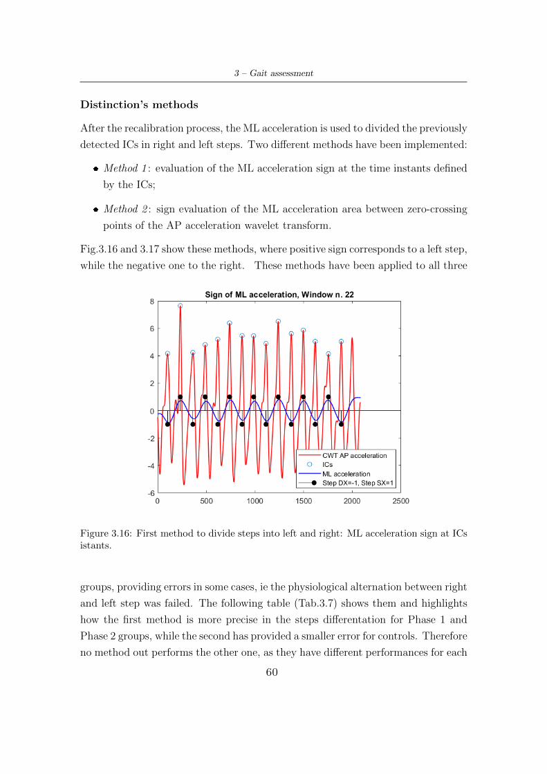
3 – Gait assessment
Distinction’s methods
After the recalibration process, the ML acceleration is used to divided the previously
detected ICs in right and left steps. Two different methods have been implemented:
� Method 1 : evaluation of the ML acceleration sign at the time instants defined
by the ICs;
� Method 2 : sign evaluation of the ML acceleration area between zero-crossing
points of the AP acceleration wavelet transform.
Fig.3.16 and 3.17 show these methods, where positive sign corresponds to a left step,
while the negative one to the right. These methods have been applied to all three
Figure 3.16: First method to divide steps into left and right: ML acceleration sign at ICsistants.
groups, providing errors in some cases, ie the physiological alternation between right
and left step was failed. The following table (Tab.3.7) shows them and highlights
how the first method is more precise in the steps differentation for Phase 1 and
Phase 2 groups, while the second has provided a smaller error for controls. Therefore
no method out performs the other one, as they have different performances for each
60
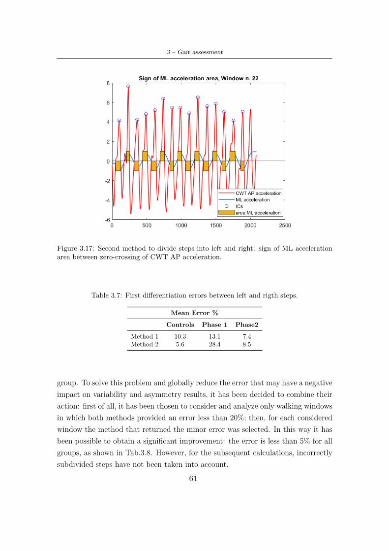
3 – Gait assessment
Figure 3.17: Second method to divide steps into left and right: sign of ML accelerationarea between zero-crossing of CWT AP acceleration.
Table 3.7: First differentiation errors between left and rigth steps.
Mean Error %
Controls Phase 1 Phase2
Method 1 10.3 13.1 7.4Method 2 5.6 28.4 8.5
group. To solve this problem and globally reduce the error that may have a negative
impact on variability and asymmetry results, it has been decided to combine their
action: first of all, it has been chosen to consider and analyze only walking windows
in which both methods provided an error less than 20%; then, for each considered
window the method that returned the minor error was selected. In this way it has
been possible to obtain a significant improvement: the error is less than 5% for all
groups, as shown in Tab.3.8. However, for the subsequent calculations, incorrectly
subdivided steps have not been taken into account.
61
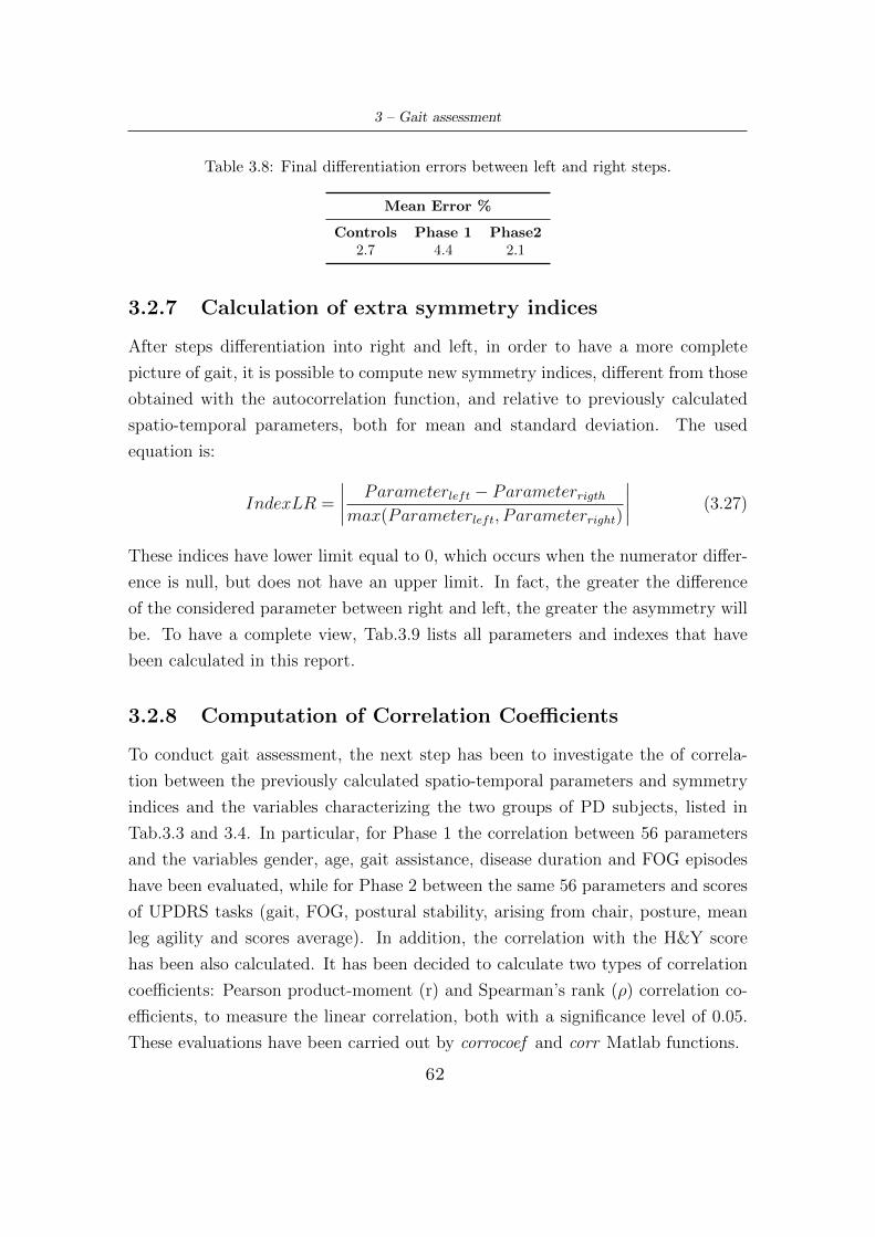
3 – Gait assessment
Table 3.8: Final differentiation errors between left and right steps.
Mean Error %
Controls Phase 1 Phase22.7 4.4 2.1
3.2.7 Calculation of extra symmetry indices
After steps differentiation into right and left, in order to have a more complete
picture of gait, it is possible to compute new symmetry indices, different from those
obtained with the autocorrelation function, and relative to previously calculated
spatio-temporal parameters, both for mean and standard deviation. The used
equation is:
IndexLR =
∣∣∣∣ Parameterleft − Parameterrigthmax(Parameterleft, Parameterright)
∣∣∣∣ (3.27)
These indices have lower limit equal to 0, which occurs when the numerator differ-
ence is null, but does not have an upper limit. In fact, the greater the difference
of the considered parameter between right and left, the greater the asymmetry will
be. To have a complete view, Tab.3.9 lists all parameters and indexes that have
been calculated in this report.
3.2.8 Computation of Correlation Coefficients
To conduct gait assessment, the next step has been to investigate the of correla-
tion between the previously calculated spatio-temporal parameters and symmetry
indices and the variables characterizing the two groups of PD subjects, listed in
Tab.3.3 and 3.4. In particular, for Phase 1 the correlation between 56 parameters
and the variables gender, age, gait assistance, disease duration and FOG episodes
have been evaluated, while for Phase 2 between the same 56 parameters and scores
of UPDRS tasks (gait, FOG, postural stability, arising from chair, posture, mean
leg agility and scores average). In addition, the correlation with the H&Y score
has been also calculated. It has been decided to calculate two types of correlation
coefficients: Pearson product-moment (r) and Spearman’s rank (ρ) correlation co-
efficients, to measure the linear correlation, both with a significance level of 0.05.
These evaluations have been carried out by corrocoef and corr Matlab functions.
62
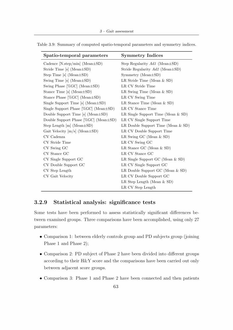
3 – Gait assessment
Table 3.9: Summary of computed spatio-temporal parameters and symmetry indices.
Spatio-temporal parameters Symmetry Indices
Cadence [N.step/min] (Mean±SD) Step Regularity Ad1 (Mean±SD)
Stride Time [s] (Mean±SD) Stride Regularity Ad2 (Mean±SD)
Step Time [s] (Mean±SD) Symmetry (Mean±SD)
Swing Time [s] (Mean±SD) LR Stride Time (Mean & SD)
Swing Phase [%GC] (Mean±SD) LR CV Stride Time
Stance Time [s] (Mean±SD) LR Swing Time (Mean & SD)
Stance Phase [%GC] (Mean±SD) LR CV Swing Time
Single Support Time [s] (Mean±SD) LR Stance Time (Mean & SD)
Single Support Phase [%GC] (Mean±SD) LR CV Stance Time
Double Support Time [s] (Mean±SD) LR Single Support Time (Mean & SD)
Double Support Phase [%GC] (Mean±SD) LR CV Single Support Time
Step Length [m] (Mean±SD) LR Double Support Time (Mean & SD)
Gait Velocity [m/s] (Mean±SD) LR CV Double Support Time
CV Cadenza LR Swing GC (Mean & SD)
CV Stride Time LR CV Swing GC
CV Swing GC LR Stance GC (Mean & SD)
CV Stance GC LR CV Stance GC
CV Single Support GC LR Single Support GC (Mean & SD)
CV Double Support GC LR CV Single Support GC
CV Step Length LR Double Support GC (Mean & SD)
CV Gait Velocity LR CV Double Support GC
LR Step Length (Mean & SD)
LR CV Step Length
3.2.9 Statistical analysis: significance tests
Some tests have been performed to assess statistically significant differences be-
tween examined groups. Three comparisons have been accomplished, using only 27
parameters:
� Comparison 1: between elderly controls group and PD subjects group (joining
Phase 1 and Phase 2);
� Comparison 2: PD subject of Phase 2 have been divided into different groups
according to their H&Y score and the comparisons have been carried out only
between adjacent score groups.
� Comparison 3: Phase 1 and Phase 2 have been connected and then patients
63
3 – Gait assessment
have been divided into subjects that manifest FOG episodes (YFOG), do not
show these episodes (NFOG) or have hesitation (HES). Then comparisons
between all groups have been accomplished.
Depending on the data distribution of each parameter, different strategies have
been performed:
1. If the parameter at hand had normal distributions for both groups indipendent
T-test was carried out, through Matlab ttest2 function with significance level
of 0.05. The distributions have been investigated by lillietest Matlab function
and also by a visual inspection, as this function does not take into account
skewness.
2. If the parameter had non-normal but continuos distributions for both groups
or if one distribution was normal and the other non-normal but continuos, the
Wilcoxon test has been accomplished through Matlab runksum function with
significance level of 0.05.
3. If parameter has at least one discontinuos distribution, no test has been con-
ducted.
64
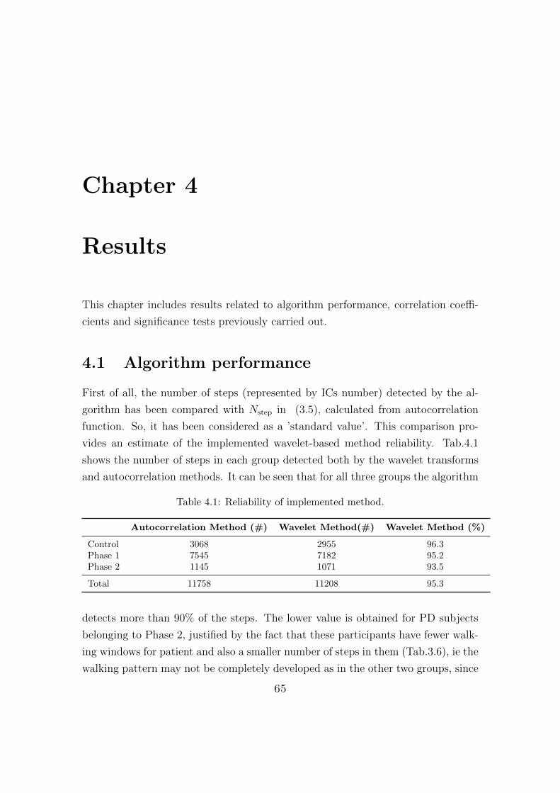
Chapter 4
Results
This chapter includes results related to algorithm performance, correlation coeffi-
cients and significance tests previously carried out.
4.1 Algorithm performance
First of all, the number of steps (represented by ICs number) detected by the al-
gorithm has been compared with Nstep in (3.5), calculated from autocorrelation
function. So, it has been considered as a ’standard value’. This comparison pro-
vides an estimate of the implemented wavelet-based method reliability. Tab.4.1
shows the number of steps in each group detected both by the wavelet transforms
and autocorrelation methods. It can be seen that for all three groups the algorithm
Table 4.1: Reliability of implemented method.
Autocorrelation Method (#) Wavelet Method(#) Wavelet Method (%)
Control 3068 2955 96.3Phase 1 7545 7182 95.2Phase 2 1145 1071 93.5
Total 11758 11208 95.3
detects more than 90% of the steps. The lower value is obtained for PD subjects
belonging to Phase 2, justified by the fact that these participants have fewer walk-
ing windows for patient and also a smaller number of steps in them (Tab.3.6), ie the
walking pattern may not be completely developed as in the other two groups, since
65
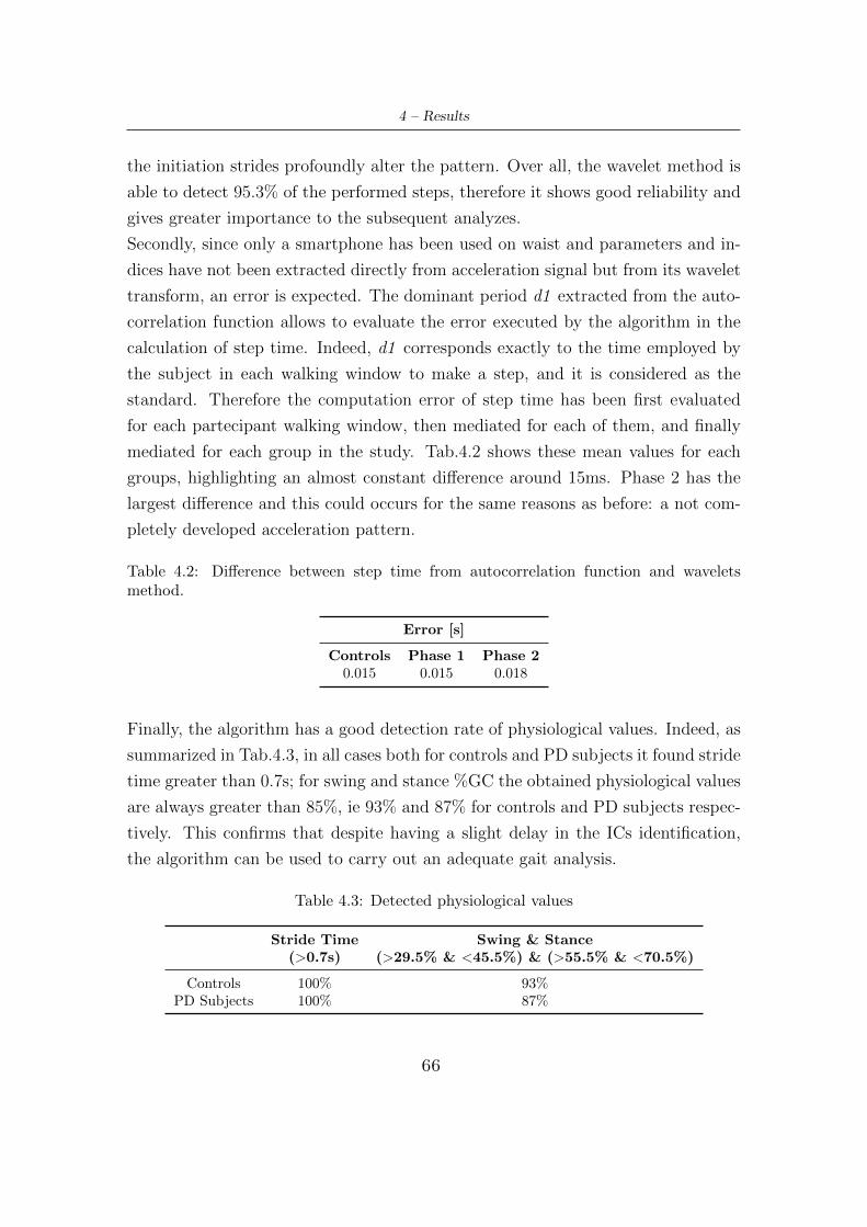
4 – Results
the initiation strides profoundly alter the pattern. Over all, the wavelet method is
able to detect 95.3% of the performed steps, therefore it shows good reliability and
gives greater importance to the subsequent analyzes.
Secondly, since only a smartphone has been used on waist and parameters and in-
dices have not been extracted directly from acceleration signal but from its wavelet
transform, an error is expected. The dominant period d1 extracted from the auto-
correlation function allows to evaluate the error executed by the algorithm in the
calculation of step time. Indeed, d1 corresponds exactly to the time employed by
the subject in each walking window to make a step, and it is considered as the
standard. Therefore the computation error of step time has been first evaluated
for each partecipant walking window, then mediated for each of them, and finally
mediated for each group in the study. Tab.4.2 shows these mean values for each
groups, highlighting an almost constant difference around 15ms. Phase 2 has the
largest difference and this could occurs for the same reasons as before: a not com-
pletely developed acceleration pattern.
Table 4.2: Difference between step time from autocorrelation function and waveletsmethod.
Error [s]
Controls Phase 1 Phase 20.015 0.015 0.018
Finally, the algorithm has a good detection rate of physiological values. Indeed, as
summarized in Tab.4.3, in all cases both for controls and PD subjects it found stride
time greater than 0.7s; for swing and stance %GC the obtained physiological values
are always greater than 85%, ie 93% and 87% for controls and PD subjects respec-
tively. This confirms that despite having a slight delay in the ICs identification,
the algorithm can be used to carry out an adequate gait analysis.
Table 4.3: Detected physiological values
Stride Time Swing & Stance(>0.7s) (>29.5% & <45.5%) & (>55.5% & <70.5%)
Controls 100% 93%PD Subjects 100% 87%
66
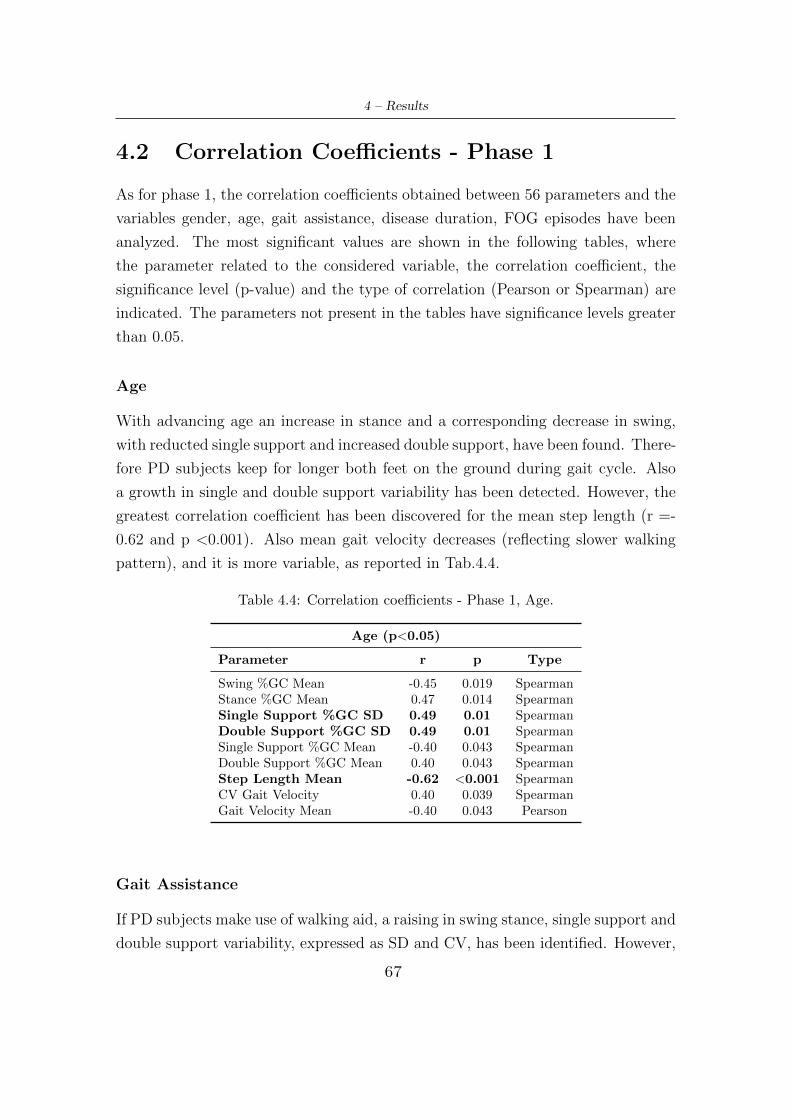
4 – Results
4.2 Correlation Coefficients - Phase 1
As for phase 1, the correlation coefficients obtained between 56 parameters and the
variables gender, age, gait assistance, disease duration, FOG episodes have been
analyzed. The most significant values are shown in the following tables, where
the parameter related to the considered variable, the correlation coefficient, the
significance level (p-value) and the type of correlation (Pearson or Spearman) are
indicated. The parameters not present in the tables have significance levels greater
than 0.05.
Age
With advancing age an increase in stance and a corresponding decrease in swing,
with reducted single support and increased double support, have been found. There-
fore PD subjects keep for longer both feet on the ground during gait cycle. Also
a growth in single and double support variability has been detected. However, the
greatest correlation coefficient has been discovered for the mean step length (r =-
0.62 and p <0.001). Also mean gait velocity decreases (reflecting slower walking
pattern), and it is more variable, as reported in Tab.4.4.
Table 4.4: Correlation coefficients - Phase 1, Age.
Age (p<0.05)
Parameter r p Type
Swing %GC Mean -0.45 0.019 SpearmanStance %GC Mean 0.47 0.014 SpearmanSingle Support %GC SD 0.49 0.01 SpearmanDouble Support %GC SD 0.49 0.01 SpearmanSingle Support %GC Mean -0.40 0.043 SpearmanDouble Support %GC Mean 0.40 0.043 SpearmanStep Length Mean -0.62 <0.001 SpearmanCV Gait Velocity 0.40 0.039 SpearmanGait Velocity Mean -0.40 0.043 Pearson
Gait Assistance
If PD subjects make use of walking aid, a raising in swing stance, single support and
double support variability, expressed as SD and CV, has been identified. However,
67
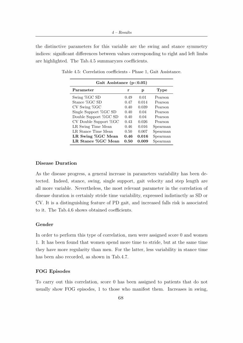
4 – Results
the distinctive parameters for this variable are the swing and stance symmetry
indices: significant differences between values corresponding to right and left limbs
are highlighted. The Tab.4.5 summaryzes coefficients.
Table 4.5: Correlation coefficients - Phase 1, Gait Assistance.
Gait Assistance (p<0.05)
Parameter r p Type
Swing %GC SD 0.49 0.01 PearsonStance %GC SD 0.47 0.014 PearsonCV Swing %GC 0.40 0.039 PearsonSingle Support %GC SD 0.40 0.04 PearsonDouble Support %GC SD 0.40 0.04 PearsonCV Double Support %GC 0.43 0.026 PearsonLR Swing Time Mean 0.46 0.016 SpearmanLR Stance Time Mean 0.50 0.007 SpearmanLR Swing %GC Mean 0.46 0.016 SpearmanLR Stance %GC Mean 0.50 0.009 Spearman
Disease Duration
As the disease progress, a general increase in parameters variability has been de-
tected. Indeed, stance, swing, single support, gait velocity and step length are
all more variable. Nevertheless, the most relevant parameter in the correlation of
disease duration is certainly stride time variability, expressed indistinctly as SD or
CV. It is a distinguishing feature of PD gait, and increased falls risk is associated
to it. The Tab.4.6 shows obtained coefficients.
Gender
In order to perform this type of correlation, men were assigned score 0 and women
1. It has been found that women spend more time to stride, but at the same time
they have more regularity than men. For the latter, less variability in stance time
has been also recorded, as shown in Tab.4.7.
FOG Episodes
To carry out this correlation, score 0 has been assigned to patients that do not
usually show FOG episodes, 1 to those who manifest them. Increases in swing,
68
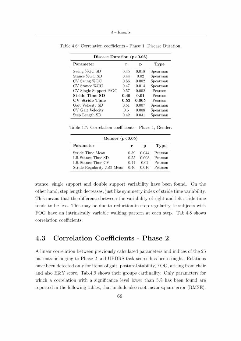
4 – Results
Table 4.6: Correlation coefficients - Phase 1, Disease Duration.
Disease Duration (p<0.05)
Parameter r p Type
Swing %GC SD 0.45 0.018 SpearmanStance %GC SD 0.44 0.02 SpearmanCV Swing %GC 0.56 0.002 SpearmanCV Stance %GC 0.47 0.014 SpearmanCV Single Support %GC 0.57 0.002 PearsonStride Time SD 0.49 0.01 PearsonCV Stride Time 0.53 0.005 PearsonGait Velocity SD 0.51 0.007 SpearmanCV Gait Velocity 0.5 0.008 SpearmanStep Length SD 0.42 0.031 Spearman
Table 4.7: Correlation coefficients - Phase 1, Gender.
Gender (p<0.05)
Parameter r p Type
Stride Time Mean 0.39 0.044 PearsonLR Stance Time SD 0.55 0.003 PearsonLR Stance Time CV 0.44 0.02 PearsonStride Regularity Ad2 Mean 0.46 0.016 Pearson
stance, single support and double support variability have been found. On the
other hand, step length decreases, just like symmetry index of stride time variability.
This means that the difference between the variability of right and left stride time
tends to be less. This may be due to reduction in step regularity, ie subjects with
FOG have an intrinsically variable walking pattern at each step. Tab.4.8 shows
correlation coefficients.
4.3 Correlation Coefficients - Phase 2
A linear correlation between previously calculated parameters and indices of the 25
patients belonging to Phase 2 and UPDRS task scores has been sought. Relations
have been detected only for items of gait, postural stability, FOG, arising from chair
and also H&Y score. Tab.4.9 shows their groups cardinality. Only parameters for
which a correlation with a significance level lower than 5% has been found are
reported in the following tables, that include also root-mean-square-error (RMSE).
69
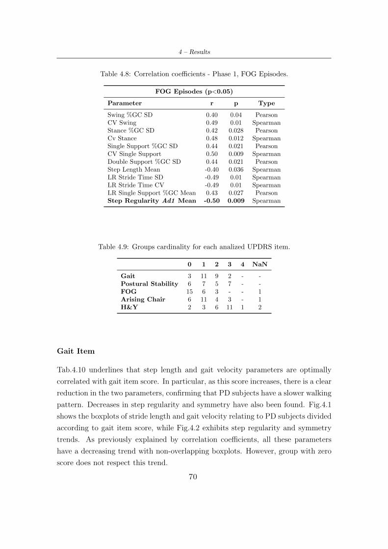
4 – Results
Table 4.8: Correlation coefficients - Phase 1, FOG Episodes.
FOG Episodes (p<0.05)
Parameter r p Type
Swing %GC SD 0.40 0.04 PearsonCV Swing 0.49 0.01 SpearmanStance %GC SD 0.42 0.028 PearsonCv Stance 0.48 0.012 SpearmanSingle Support %GC SD 0.44 0.021 PearsonCV Single Support 0.50 0.009 SpearmanDouble Support %GC SD 0.44 0.021 PearsonStep Length Mean -0.40 0.036 SpearmanLR Stride Time SD -0.49 0.01 SpearmanLR Stride Time CV -0.49 0.01 SpearmanLR Single Support %GC Mean 0.43 0.027 PearsonStep Regularity Ad1 Mean -0.50 0.009 Spearman
Table 4.9: Groups cardinality for each analized UPDRS item.
0 1 2 3 4 NaN
Gait 3 11 9 2 - -Postural Stability 6 7 5 7 - -FOG 15 6 3 - - 1Arising Chair 6 11 4 3 - 1H&Y 2 3 6 11 1 2
Gait Item
Tab.4.10 underlines that step length and gait velocity parameters are optimally
correlated with gait item score. In particular, as this score increases, there is a clear
reduction in the two parameters, confirming that PD subjects have a slower walking
pattern. Decreases in step regularity and symmetry have also been found. Fig.4.1
shows the boxplots of stride length and gait velocity relating to PD subjects divided
according to gait item score, while Fig.4.2 exhibits step regularity and symmetry
trends. As previously explained by correlation coefficients, all these parameters
have a decreasing trend with non-overlapping boxplots. However, group with zero
score does not respect this trend.
70
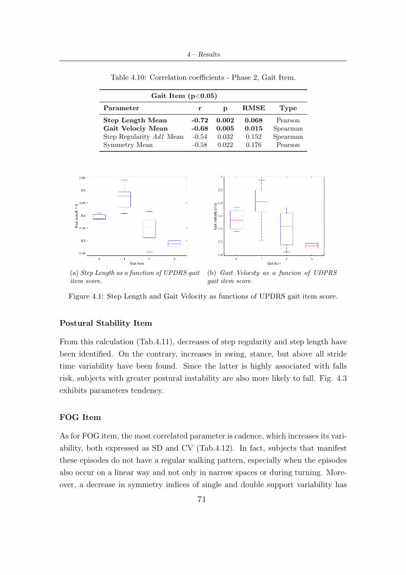
4 – Results
Table 4.10: Correlation coefficients - Phase 2, Gait Item.
Gait Item (p<0.05)
Parameter r p RMSE Type
Step Length Mean -0.72 0.002 0.068 PearsonGait Velociy Mean -0.68 0.005 0.015 SpearmanStep Regularity Ad1 Mean -0.54 0.032 0.152 SpearmanSymmetry Mean -0.58 0.022 0.176 Pearson
(a) Step Length as a function of UPDRS gaititem score.
(b) Gait Velocity as a funcion of UDPRSgait item score.
Figure 4.1: Step Length and Gait Velocity as functions of UPDRS gait item score.
Postural Stability Item
From this calculation (Tab.4.11), decreases of step regularity and step length have
been identified. On the contrary, increases in swing, stance, but above all stride
time variability have been found. Since the latter is highly associated with falls
risk, subjects with greater postural instability are also more likely to fall. Fig. 4.3
exhibits parameters tendency.
FOG Item
As for FOG item, the most correlated parameter is cadence, which increases its vari-
ability, both expressed as SD and CV (Tab.4.12). In fact, subjects that manifest
these episodes do not have a regular walking pattern, especially when the episodes
also occur on a linear way and not only in narrow spaces or during turning. More-
over, a decrease in symmetry indices of single and double support variability has
71
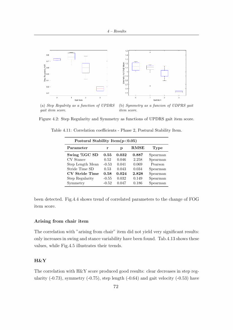
4 – Results
(a) Step Regulrity as a function of UPDRSgait item score.
(b) Symmetry as a funcion of UDPRS gaititem score.
Figure 4.2: Step Regularity and Symmetry as functions of UPDRS gait item score.
Table 4.11: Correlation coefficients - Phase 2, Postural Stability Item.
Postural Stability Item(p<0.05)
Parameter r p RMSE Type
Swing %GC SD 0.55 0.032 0.887 SpearmanCV Stance 0.52 0.046 2.258 SpearmanStep Length Mean -0.53 0.041 0.069 PearsonStride Time SD 0.53 0.043 0.034 SpearmanCV Stride Time 0.58 0.024 2.828 SpearmanStep Regularity -0.55 0.032 0.149 SpearmanSymmetry -0.52 0.047 0.186 Spearman
been detected. Fig.4.4 shows trend of correlated parameters to the change of FOG
item score.
Arising from chair item
The correlation with ”arising from chair” item did not yield very significant results:
only increases in swing and stance variability have been found. Tab.4.13 shows these
values, while Fig.4.5 illustrates their trends.
H&Y
The correlation with H&Y score produced good results: clear decreases in step reg-
ularity (-0.73), symmetry (-0.75), step length (-0.64) and gait velocity (-0.53) have
72
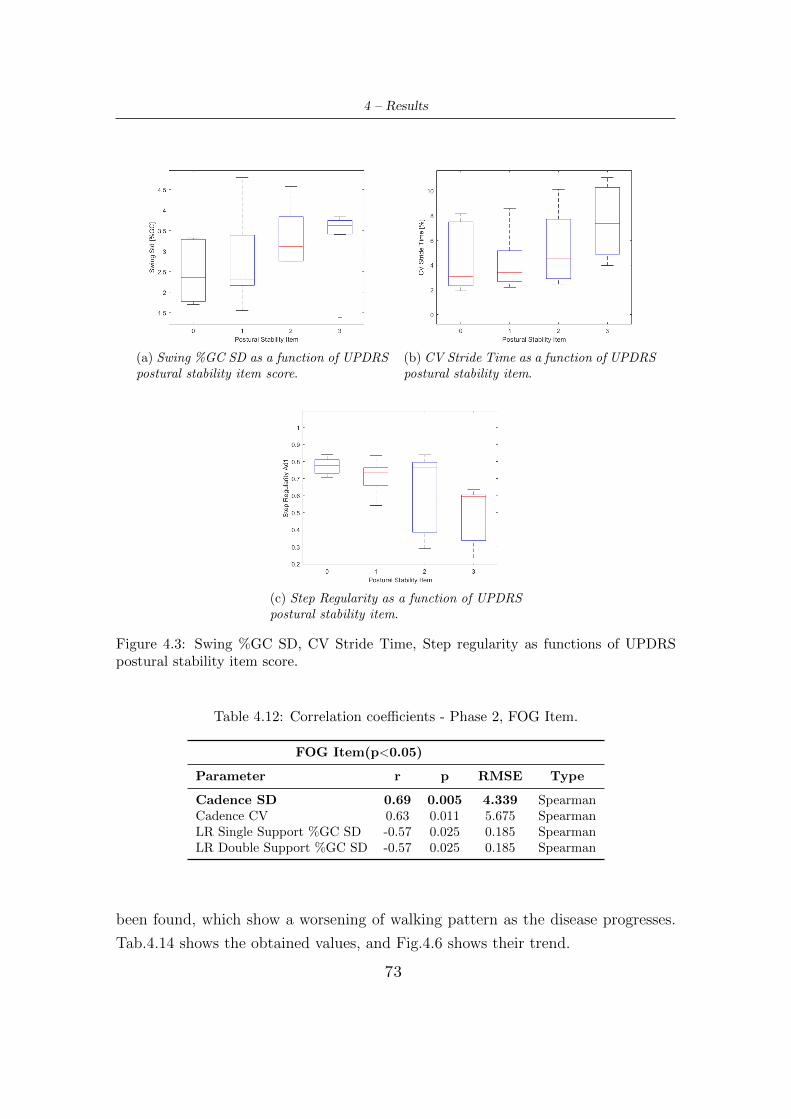
4 – Results
(a) Swing %GC SD as a function of UPDRSpostural stability item score.
(b) CV Stride Time as a function of UPDRSpostural stability item.
(c) Step Regularity as a function of UPDRSpostural stability item.
Figure 4.3: Swing %GC SD, CV Stride Time, Step regularity as functions of UPDRSpostural stability item score.
Table 4.12: Correlation coefficients - Phase 2, FOG Item.
FOG Item(p<0.05)
Parameter r p RMSE Type
Cadence SD 0.69 0.005 4.339 SpearmanCadence CV 0.63 0.011 5.675 SpearmanLR Single Support %GC SD -0.57 0.025 0.185 SpearmanLR Double Support %GC SD -0.57 0.025 0.185 Spearman
been found, which show a worsening of walking pattern as the disease progresses.
Tab.4.14 shows the obtained values, and Fig.4.6 shows their trend.
73
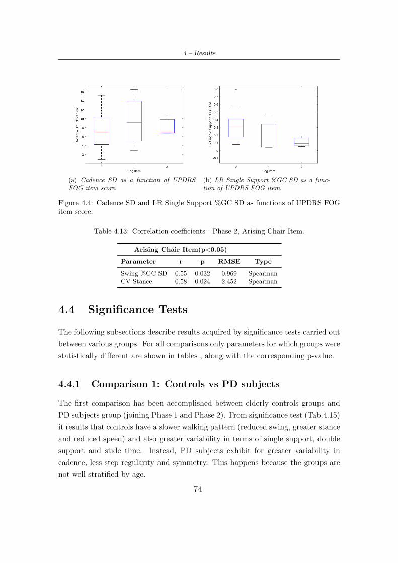
4 – Results
(a) Cadence SD as a function of UPDRSFOG item score.
(b) LR Single Support %GC SD as a func-tion of UPDRS FOG item.
Figure 4.4: Cadence SD and LR Single Support %GC SD as functions of UPDRS FOGitem score.
Table 4.13: Correlation coefficients - Phase 2, Arising Chair Item.
Arising Chair Item(p<0.05)
Parameter r p RMSE Type
Swing %GC SD 0.55 0.032 0.969 SpearmanCV Stance 0.58 0.024 2.452 Spearman
4.4 Significance Tests
The following subsections describe results acquired by significance tests carried out
between various groups. For all comparisons only parameters for which groups were
statistically different are shown in tables , along with the corresponding p-value.
4.4.1 Comparison 1: Controls vs PD subjects
The first comparison has been accomplished between elderly controls groups and
PD subjects group (joining Phase 1 and Phase 2). From significance test (Tab.4.15)
it results that controls have a slower walking pattern (reduced swing, greater stance
and reduced speed) and also greater variability in terms of single support, double
support and stide time. Instead, PD subjects exhibit for greater variability in
cadence, less step regularity and symmetry. This happens because the groups are
not well stratified by age.
74
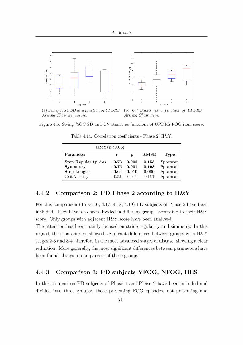
4 – Results
(a) Swing %GC SD as a function of UPDRSArising Chair item score.
(b) CV Stance as a function of UPDRSArising Chair item.
Figure 4.5: Swing %GC SD and CV stance as functions of UPDRS FOG item score.
Table 4.14: Correlation coefficients - Phase 2, H&Y.
H&Y(p<0.05)
Parameter r p RMSE Type
Step Regularity Ad1 -0.73 0.002 0.153 SpearmanSymmetry -0.75 0.001 0.193 SpearmanStep Length -0.64 0.010 0.080 SpearmanGait Velocity -0.53 0.044 0.166 Spearman
4.4.2 Comparison 2: PD Phase 2 according to H&Y
For this comparison (Tab.4.16, 4.17, 4.18, 4.19) PD subjects of Phase 2 have been
included. They have also been divided in different groups, according to their H&Y
score. Only groups with adjacent H&Y score have been analysed.
The attention has been mainly focused on stride regularity and simmetry. In this
regard, these parameters showed significant differences between groups with H&Y
stages 2-3 and 3-4, therefore in the most advanced stages of disease, showing a clear
reduction. More generally, the most significant differences between parameters have
been found always in comparison of these groups.
4.4.3 Comparison 3: PD subjects YFOG, NFOG, HES
In this comparison PD subjects of Phase 1 and Phase 2 have been included and
divided into three groups: those presenting FOG episodes, not presenting and
75
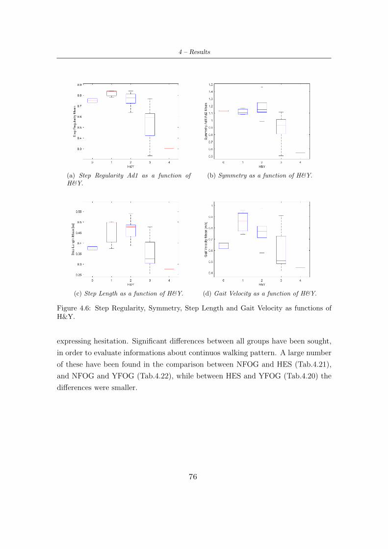
4 – Results
(a) Step Regularity Ad1 as a function ofH&Y.
(b) Symmetry as a function of H&Y.
(c) Step Length as a function of H&Y. (d) Gait Velocity as a function of H&Y.
Figure 4.6: Step Regularity, Symmetry, Step Length and Gait Velocity as functions ofH&Y.
expressing hesitation. Significant differences between all groups have been sought,
in order to evaluate informations about continuos walking pattern. A large number
of these have been found in the comparison between NFOG and HES (Tab.4.21),
and NFOG and YFOG (Tab.4.22), while between HES and YFOG (Tab.4.20) the
differences were smaller.
76
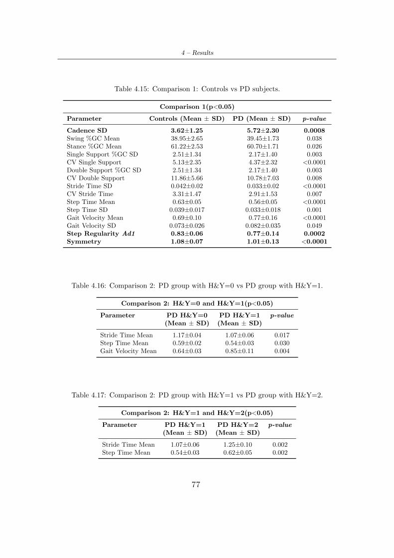
4 – Results
Table 4.15: Comparison 1: Controls vs PD subjects.
Comparison 1(p<0.05)
Parameter Controls (Mean ± SD) PD (Mean ± SD) p-value
Cadence SD 3.62±1.25 5.72±2.30 0.0008Swing %GC Mean 38.95±2.65 39.45±1.73 0.038Stance %GC Mean 61.22±2.53 60.70±1.71 0.026Single Support %GC SD 2.51±1.34 2.17±1.40 0.003CV Single Support 5.13±2.35 4.37±2.32 <0.0001Double Support %GC SD 2.51±1.34 2.17±1.40 0.003CV Double Support 11.86±5.66 10.78±7.03 0.008Stride Time SD 0.042±0.02 0.033±0.02 <0.0001CV Stride Time 3.31±1.47 2.91±1.53 0.007Step Time Mean 0.63±0.05 0.56±0.05 <0.0001Step Time SD 0.039±0.017 0.033±0.018 0.001Gait Velocity Mean 0.69±0.10 0.77±0.16 <0.0001Gait Velocity SD 0.073±0.026 0.082±0.035 0.049Step Regularity Ad1 0.83±0.06 0.77±0.14 0.0002Symmetry 1.08±0.07 1.01±0.13 <0.0001
Table 4.16: Comparison 2: PD group with H&Y=0 vs PD group with H&Y=1.
Comparison 2: H&Y=0 and H&Y=1(p<0.05)
Parameter PD H&Y=0 PD H&Y=1 p-value(Mean ± SD) (Mean ± SD)
Stride Time Mean 1.17±0.04 1.07±0.06 0.017Step Time Mean 0.59±0.02 0.54±0.03 0.030Gait Velocity Mean 0.64±0.03 0.85±0.11 0.004
Table 4.17: Comparison 2: PD group with H&Y=1 vs PD group with H&Y=2.
Comparison 2: H&Y=1 and H&Y=2(p<0.05)
Parameter PD H&Y=1 PD H&Y=2 p-value(Mean ± SD) (Mean ± SD)
Stride Time Mean 1.07±0.06 1.25±0.10 0.002Step Time Mean 0.54±0.03 0.62±0.05 0.002
77
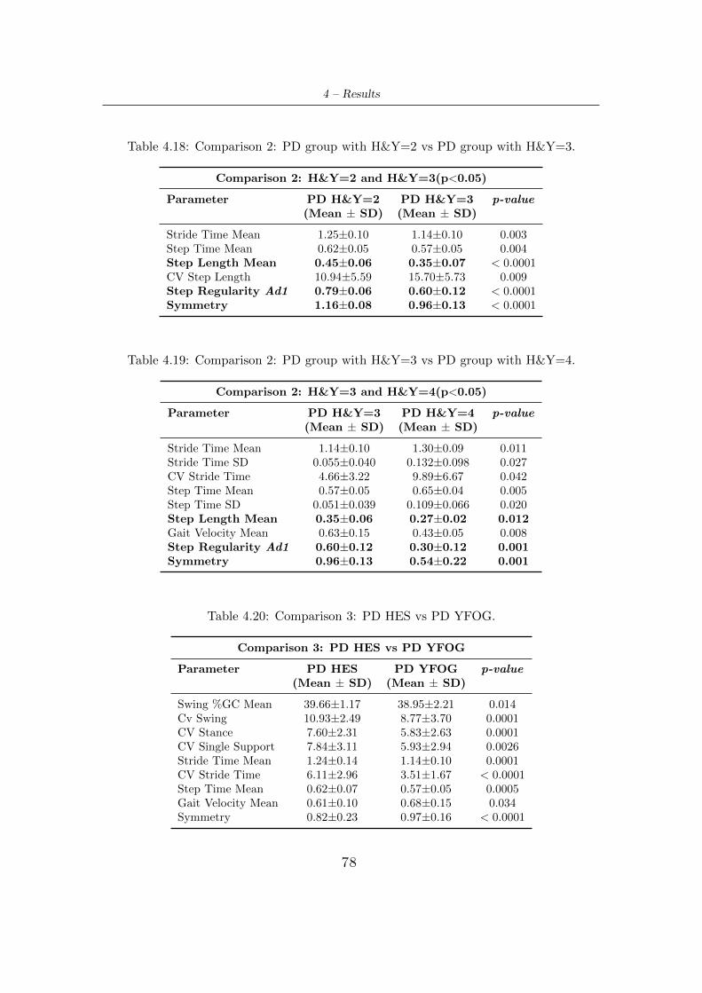
4 – Results
Table 4.18: Comparison 2: PD group with H&Y=2 vs PD group with H&Y=3.
Comparison 2: H&Y=2 and H&Y=3(p<0.05)
Parameter PD H&Y=2 PD H&Y=3 p-value(Mean ± SD) (Mean ± SD)
Stride Time Mean 1.25±0.10 1.14±0.10 0.003Step Time Mean 0.62±0.05 0.57±0.05 0.004Step Length Mean 0.45±0.06 0.35±0.07 < 0.0001CV Step Length 10.94±5.59 15.70±5.73 0.009Step Regularity Ad1 0.79±0.06 0.60±0.12 < 0.0001Symmetry 1.16±0.08 0.96±0.13 < 0.0001
Table 4.19: Comparison 2: PD group with H&Y=3 vs PD group with H&Y=4.
Comparison 2: H&Y=3 and H&Y=4(p<0.05)
Parameter PD H&Y=3 PD H&Y=4 p-value(Mean ± SD) (Mean ± SD)
Stride Time Mean 1.14±0.10 1.30±0.09 0.011Stride Time SD 0.055±0.040 0.132±0.098 0.027CV Stride Time 4.66±3.22 9.89±6.67 0.042Step Time Mean 0.57±0.05 0.65±0.04 0.005Step Time SD 0.051±0.039 0.109±0.066 0.020Step Length Mean 0.35±0.06 0.27±0.02 0.012Gait Velocity Mean 0.63±0.15 0.43±0.05 0.008Step Regularity Ad1 0.60±0.12 0.30±0.12 0.001Symmetry 0.96±0.13 0.54±0.22 0.001
Table 4.20: Comparison 3: PD HES vs PD YFOG.
Comparison 3: PD HES vs PD YFOG
Parameter PD HES PD YFOG p-value(Mean ± SD) (Mean ± SD)
Swing %GC Mean 39.66±1.17 38.95±2.21 0.014Cv Swing 10.93±2.49 8.77±3.70 0.0001CV Stance 7.60±2.31 5.83±2.63 0.0001CV Single Support 7.84±3.11 5.93±2.94 0.0026Stride Time Mean 1.24±0.14 1.14±0.10 0.0001CV Stride Time 6.11±2.96 3.51±1.67 < 0.0001Step Time Mean 0.62±0.07 0.57±0.05 0.0005Gait Velocity Mean 0.61±0.10 0.68±0.15 0.034Symmetry 0.82±0.23 0.97±0.16 < 0.0001
78
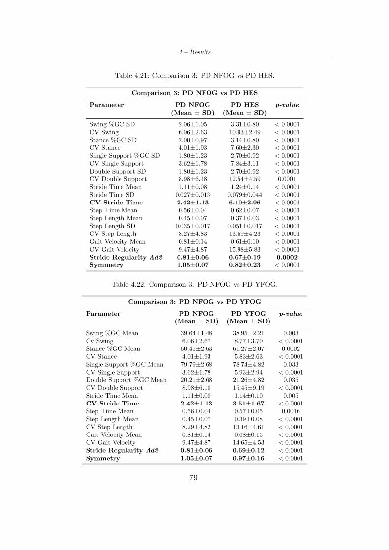
4 – Results
Table 4.21: Comparison 3: PD NFOG vs PD HES.
Comparison 3: PD NFOG vs PD HES
Parameter PD NFOG PD HES p-value(Mean ± SD) (Mean ± SD)
Swing %GC SD 2.06±1.05 3.31±0.80 < 0.0001CV Swing 6.06±2.63 10.93±2.49 < 0.0001Stance %GC SD 2.00±0.97 3.14±0.80 < 0.0001CV Stance 4.01±1.93 7.60±2.30 < 0.0001Single Support %GC SD 1.80±1.23 2.70±0.92 < 0.0001CV Single Support 3.62±1.78 7.84±3.11 < 0.0001Double Support SD 1.80±1.23 2.70±0.92 < 0.0001CV Double Support 8.98±6.18 12.54±4.59 0.0001Stride Time Mean 1.11±0.08 1.24±0.14 < 0.0001Stride Time SD 0.027±0.013 0.079±0.044 < 0.0001CV Stride Time 2.42±1.13 6.10±2.96 < 0.0001Step Time Mean 0.56±0.04 0.62±0.07 < 0.0001Step Length Mean 0.45±0.07 0.37±0.03 < 0.0001Step Length SD 0.035±0.017 0.051±0.017 < 0.0001CV Step Length 8.27±4.83 13.69±4.23 < 0.0001Gait Velocity Mean 0.81±0.14 0.61±0.10 < 0.0001CV Gait Velocity 9.47±4.87 15.98±5.83 < 0.0001Stride Regularity Ad2 0.81±0.06 0.67±0.19 0.0002Symmetry 1.05±0.07 0.82±0.23 < 0.0001
Table 4.22: Comparison 3: PD NFOG vs PD YFOG.
Comparison 3: PD NFOG vs PD YFOG
Parameter PD NFOG PD YFOG p-value(Mean ± SD) (Mean ± SD)
Swing %GC Mean 39.64±1.48 38.95±2.21 0.003Cv Swing 6.06±2.67 8.77±3.70 < 0.0001Stance %GC Mean 60.45±2.63 61.27±2.07 0.0002CV Stance 4.01±1.93 5.83±2.63 < 0.0001Single Support %GC Mean 79.79±2.68 78.74±4.82 0.033CV Single Support 3.62±1.78 5.93±2.94 < 0.0001Double Support %GC Mean 20.21±2.68 21.26±4.82 0.035CV Double Support 8.98±6.18 15.45±9.19 < 0.0001Stride Time Mean 1.11±0.08 1.14±0.10 0.005CV Stride Time 2.42±1.13 3.51±1.67 < 0.0001Step Time Mean 0.56±0.04 0.57±0.05 0.0016Step Length Mean 0.45±0.07 0.39±0.08 < 0.0001CV Step Length 8.29±4.82 13.16±4.61 < 0.0001Gait Velocity Mean 0.81±0.14 0.68±0.15 < 0.0001CV Gait Velocity 9.47±4.87 14.65±4.53 < 0.0001Stride Regularity Ad2 0.81±0.06 0.69±0.12 < 0.0001Symmetry 1.05±0.07 0.97±0.16 < 0.0001
79
Chapter 5
Discussion
The correlations for PD subjects of Phase 1 mainly provide general information on
the disease, both regarding continuous and episodic motor disturbances. In partic-
ular, correlations with subject age and disease duration are of considerable interest
for continuous impairment. As for age, a large number of PD walking features
have been detected: a definite reduction in step length and gait velocity has been
observed, followed by increase in stance at swing expense. These results clearly
indicate the presence of a slower and compromised, non-rhythmic walking pattern,
since gait velocity increases its variability. Increases in single and double support
variability have been also identified. Therefore, globally, it is possible to conclude
that, with age progression, motor symptoms related to gait impairment tend to
worsen, where the reduced and shorter step length (which has the greatest correla-
tion coefficient, -0.62) could be the triggering cause of the other gait distubances, as
reduced gait velocity and increased time with the feet on the ground. These results
agrees with those present in literature, as Schlachetzki et al. [82] that exposes the
same parameters trends.
The PD gait motor disturbances also include features that are not always easily
identifiable during routine clinical observation, but which can be detected by gait
analysis systems. One of these is the loss of ability to produce a steady gait rhythm,
resulting in higher stride time variability, that is a characteristic feature of gait in
PD, closely associated with risk of falls. The correlation with disease duration
shows this feature trend, both expressed as SD and CV, where their magnitude
tends to increase (0.53), as also reported by Hausdorff [34]. Stride time variability
80
5 – Discussion
is a manifestation of a general gait variability, which is also expressed by detected
increase in variability of other parameters, such as swing, stance, gait velocity and
step length.
For episodic disturbances, correlation with FOG episodes provide some useful in-
formations. First of all, reduction in step regularity has been detected (-0.50), ie
patients that manifest these episodes show a less rhytmic and consistent walking
pattern. Moreover, similar to correlation with age and disease duration, increase
in general gait variability has been found, expressed by CV or SD growth of swing,
stance, single support and double support, but also by a reduction in symmetry
indices of stride time variability. This means that gait variability is a general fea-
ture, and not primarily focused on a specific lower limb.
Correlations with gait assistance and gender provide information not related to the
general disease, but more specific to the examined cases: if PD subject uses a walk-
ing aid, there is a difference between right and left stance/swing, as expressed by
relative symmetry indexes and as it is reasonable to expect. About gender, women
seem to have a greater stride time but at the same time a higher gait regularity,
and therefore greater stability.
The UPDRS Part III is a means widely used by neurologists to evaluate motor
functionality of PD subjects, but it is affected by inter and intra rater variabil-
ity. Indeed, clinicians do not always assign the same score for an item to a given
patient. This can occur because the entries pertaining to a particular score of a
specific item are not sufficiently clear, but allows for further interpretation by neu-
rologists. Therefore, the need to quantify the UPDRS items has been felt, in order
to provide more precise and objective information that can be used by clinicians,
in addition to their experience, to assign a given score.
According to the definition of UPDRS gait item, is given a score to gait by ob-
serving mainly changes in step length and velocity. The high detected correlation
values correspond to clinician’s gait rating: they underline that step length and
gait velocity are significantly reduced (-0.72 and -0.68, respecively) in patients who
have substantial gait impairment compared to those who have a lower score (min-
imal or absent damage). The reduction of step regularity (-0.54) also confirms the
typical and highly variable gait pattern, while increase of asymmetry agrees with
the unilateral nature of the disease.
The performance in pull test determines score assigned by neurologists to postural
81
5 – Discussion
stability item. In particular, more are the steps performed by the subject to recover
posture and balance or if these are totally absent and subject falls if not supported,
higher the score will be. In addition to pull test observation, the extracted corre-
lation coefficients provide a useful supplementary information: the increase in gait
variability, expressed by swing and stance variability, step regularity and stride time
variability. The latter is related to an increased falls risk, confirming that postural
instability is highly related to these events, endangering patients and worsening
their quality of life. Instead, the reduction of step length means that the subject
takes smaller steps, transferring body weight between limbs more frequently.
Patients in a moderate stage of the disease (H&Y stage 3) show a clear reduction
of most the identifying gait parameters: step length (-0.64) and velocity (-0.53).
Also step regularity and symmetry are significantly reduced (-0.73 and -0.75, re-
spectively). The first one agrees with the fact that as the H&Y score increases,
the patient is more affected by disease and gait impairment, thus showing a greater
general gait variability. On the other hand, symmetry is partially in contrast with
H&Y scale entries. According to these, score 1 indicates unilateral involvement and
2 a bilateral. However, in patients belonging to these two groups approximately the
same symmetry value has been found, and a distinct reduction comes from score
2 onwards. This can be explained by the fact that, although the disease initially
reveals itself in a unilateral way and subsequently tends to affect both sides, nev-
ertheless it keeps a unilateral nature, ie there will be always a more affected side.
The results of gait, postural stability and H&Y correlations are consistent with
those achieved from other studies: Schlachetzki et al. [82] found PD gait characheris-
tics including short steps, shuffling gait and postural instability features, using in-
ertial sensors units attached laterally to both shoes and comparing parameters to
UPDRS gait score; Das et al.[83] obtained mean speed correlation coefficient of
-0.51 with UPDRS gait task using motion capture data; Salarian et al.[86] reported
high negative correlations between stride length and velocity with UPDRS gait
item having use of body-attached gyroscopes.
However, in this work, it has been found that subjects with scores equal to 0 do
not respect trend parameters correlated with these UPDRS item, and this may
depend on two reasons: a low population in this group or a non-precise distinction
of subjects with scores 0 and 1 by neurologists.
Regarding arising chair item, only increases in swing and stance variability have
82
5 – Discussion
been found, while about FOG item the noteworthy result is the correlation with
cadence SD that significantly intensifies (0.69). Also reduction in symmetry vari-
ability indices of single and double support has been detected. This means that
there is a tendency to have the same degree of variability on both lower limbs.
The general comparison between controls and PD subjects shows contrasting re-
sults compared to those in literature. Schlachetzki et al.[82] reported reduction
of stride length and increase of stride time, ie manifestations of a pattern with
reduced cadence and gait velocity, reflecting typical bradykinetic characteristics of
gait in PD; Wahid et al.[84] obtained higher cadence and smaller step length in
PD subjects than in controls; Sofuwa et al.[85] found lower walking velocity and
stride length, Salarian et al.[86] reported significantly different gait parameters (like
reduced velocity and stride length) between PD subject and controls.
However, in the present work, the opposite has been noted. Controls have a much
slower walking pattern than PD subjects: they show a greater swing and a lower
stance (keeping feet more time on the ground); have greater variability in single and
double support expressed as SD or CV; spend longer time to make a stride with
even greater variability (having greater falls risk), and also gait velocity and its
variability are reduced. Nevertheless, these results have a specific cause: controls
group has a mean age of 84.9 years, significantly higher than the PD subjects group
age (70.1). Therefore, it is reasonable that these participants, having an advanced
age and a reduced muscular strength, manifest a much slower walking pattern than
subjects with a distinctly inferior age, even if with PD. However, these evidences
highlight a notheworhty aspect of PD walking: despite controls have slower pattern,
PD patients exhibit statistically significant differences concering cadence variabil-
ity, step regularity and symmetry. In particular, the greater cadence variability is
confirmed as one of gait PD features, as well as highest variability to make steps,
exposing subject to greater falls possibilities. Instead, about symmetry, this has
been found significantly lower than controls, confirming again the asymmetric man-
ifestation of the disease motor symptoms.
About comparison 2, executed between groups with adjacent H&Y scores, results
confirm what has been obtained with correlation coefficients. There is a decreasing
trend of step regularity and symmetry, but this occurs only in the most advanced
stages of disease, confirming that groups with H&Y equal to 0, 1 and 2 are not well
differentiated. Therefore, even highlighting this problem, it is possible to claim
83
5 – Discussion
that most advanced stages of PD are characterized by a more variable, less stable
and non-rhythmic walking pattern and by asymmetry that continues to manifest
itself, even if the motor symptoms are widespread on both lower limbs. Also re-
ductions of step length and gait velocity have been found only in these advanced
stage, while other parameters, although presenting significant differences between
various groups, have a variable trend, like stride time and step time.
Regarding the last comparison (number 3), it shows that it is possible to clearly dis-
criminate subjects that not usually manifest FOG episodes from those who manifest
them or express hesitations, while the other two groups appear to be closer and less
distinguishable. Indeed, NFOGs express a less compromised walking pattern than
HESs: gait variability, expressed by swing, stance, single support, double support,
stride time, step length and gait velocity SD or CV is significantly lower; mean
values of stride time and step time are smaller (and therefore velocity is greater),
and finally even the rhythm of stepping and symmetry have higher values. Also
compared to YFOG group, the NFOGs have a better and faster walking pattern:
in addition to a lower gait variability, a lesser swing time (and consequently greater
stance), higher speed, better stride regularity and higher symmetry have been also
found. Instead, as for comparison between YFOGs and HESs, the latter seem to
have most compromised gait: they manifest greater variability, higher step time and
stride time, and reduced velocity and symmetry. However, this comparison should
be further investigated, also increasing HES group population which is lower com-
pared to the other two groups.
Therefore, based on this, we can claim that the most significant comparison is
between NFOGs and YFOGs. It represents a further demonstration of results pre-
viously observed in Phase 1 and Phase 2 correlations: subjects that manifest FOG
episodes have an evident and growing arrhythmicity of stepping, short steps, and
a marked increase in gait variability, expressed by swing, stance, double support,
single support. In addition, they spend more time with both feet on the ground,
as shown by increased stance and double support phases and by corresponding
decrease of swing and single support. Also raised stride time variability has been
found, emphasizing that FOG, together with postural instability, contribute to ex-
posing subject to a greater risk of falls. All these results about comparison between
NFOG and YFOG are consistent with literature: Shah et al. [87] reported same
parameters trend using pressur sensor impregnated mat and Weiss et al. [88] found
84

5 – Discussion
that freezers had decreased stride regularity compared with non-freezers.
85
Chapter 6
Conclusions
The application of wavelet transform to vertical and anteroposterior acceleration
components allows to detect 95.3% of steps perfomed by participants and to obtain
parameter values in physiological ranges. Their trend follows clinically relevant pat-
terns and confirms what is present in literature: reduced swing in favor of stance,
reduced gait velocity and step length, asymmetry, but especially increase of gait
variability. The trend of this feature has been found in all performed analyses: cor-
relations with age, disease duration, UPDRS item score, H&Y score, comparison
between controls and PD, and also between NFOG and YFOG. It is mainly rep-
resented by an increase of stride time variability and by a reduction of step/stride
regularity. Therefore, PD subjects have a less consistent, arrhythmic and less stable
walking pattern, especially in advanced stages of disease.
This work has shown that it is possible to adequately and satisfactorily perform
gait assessment in PD through wearable systems, such as a single waist-mounted
smartphone, which has the capability to detect changes of some spatio-temporal
parameters that are difficult to appreciate during a routine clinical examination.
To implement this, it is not necessary for subjects to walk long distances, as demon-
strated by Phase 2 group, whose data have been acquired in ADL-like conditions,
which makes this approach usable also in a domestic environment. It allows to
describe current motor state of PD subject, and can be also extremely useful to
monitor the progress of gait impairment, providing in this regard additional and
objective informations (also about UPDRS item) that can be employed by neurol-
ogists to modify appropriately and specific for each patient the pharmacological
86
6 – Conclusions
treatment. Furthermore, expressing good sensitivity towards the detection of gait
variability, it is also possible to predict and control the risk of falls associated with
it and postural instability, that compromise patient quality of life. Finally, hav-
ing demonstrated good performance for PD subjects with gait impairment, it can
be also used in rehabilitation environment to monitor the improvement of subject
motor conditions, or to evaluate healthy subjects gait.
87
Bibliography
[1] Dennis W. Dickson, Parkinson’s Disease and Parkinsonism: Neuropathology,
Cold Spring Harb Perspect Med, 2012.
[2] European Parkinson’s Disease Association, https://www.epda.eu.com/.
[3] A. Elbaz, L. Carcaillon, S. Kab, F. Moisan, Epidemiology of Parkinson’s
disease, Revue Neurologique Volume 172, Issue 1, January 2016, Pages 14-26.
[4] C. A. Davie, A review of Parkinson’s disease, British Medical Bulletin, 2008,
86: 109-127.
[5] Dennis W.Dickson, Neuropathology of Parkinson disease, Parkinsonism and
Related Disorders 46, 2018, S30-S33.
[6] Leonid Breydo, Jessica W. Wu, Vladimir N. Uvesky, α-Synuclein misfolding
and Parkinson’s disease, Biochimica et Biophysica Acta 1822, 2012, 261-285.
[7] Guido Alves, Elin Bjelland Forsaa, et al., Epidemiology of Parkinson’s disease,
J Neurol, 2008, 255, Suppl 5:18-32.
[8] Andrea Lee, Rebecca M. Gilbert, Epidemiology of Parkinson Disease, Neuro-
logic Clinics 34, 2016, 955-965.
[9] Sigurlaug Sveinbjornsdottir, The clinical symptoms of Parkinson’s disease, J.
Neurochem.,2016.
[10] Sonja von Campenhausen, Bernhard Bornschein, et al., Prevalence and inci-
dence of Parkinson’s disease in Europe, European Neuropsychopharmacology
15, 2005, 473-490.
[11] Lorraine V Kalia, Anthony E Lang, Parkinson’s Disease, Lancet, 2015, 386:
896-912.
[12] E.R. Dorsey, R. Constantinescu, J.P. Thompson et al., Projected number of
people with Parkinson disease in the most populous nations, 2005 through
2030, Neurology, 2007, 68, 384-386.
88
Bibliography
[13] Stephen K. Van Den Eeden, Caroline M. Tanner, et al., Incidence of Parkin-
son’s Disease: Variation by Age, Gender, and Race/Ethnicity, Am J Epi-
demiol, 2003, 157:1015-1022.
[14] Werner Poewe, Klaus Seppi, et al., Parkinson Disease, Nature reviews, Dis-
ease primers, Volume 3, Article Number 17013, 2017.
[15] Joao Massano and Kailash P. Bhatia1, Clinical Approach to Parkinson’s Dis-
ease: Features, Diagnosis, and Principles of Management, Cold Spring Harb
Perspect Med, 2012.
[16] J. Jankovic, Parkinson’s Disease: clinical features and diagnosis,J Neurol
Neurosurg Psychiatry, 2008, 79:368-376.
[17] J. Jankovic, Pathophysiology And Clinical Assessment of Parkinsonian Symp-
toms And Signs.
[18] Stanely Fahn, Description of Parkinson’s Disease as a Clinical Syndrome,
Ann. N.Y. Acad. Sci. 991: 1-14, 2003.
[19] Andrew J Lees, John Hardy, Tamas Revesz, Parkinson’s Disease, Lancet,
2009, 373: 2055-66.
[20] William Dauer and Serge Przedborski, Parkinson’s Disease: Mechanisms and
Models, Neuron, Vol. 39, 889-909, 2003.
[21] Surender Dhiman, A review of gait cycle and its parameters, International
Journal of Computational Engineering & Management, Vol. 13, July 2011.
[22] Neumann Donald A, Kinesiology of the musculoskeletal system: foundations
for physical rehabilitation, St. Louis: Mosby, 2010.
[23] Ryan P. Hubble, Geraldine A. Naughton, et al., Wearable Sensor Use for
Assessing Standing Balance and Walking Stability in People with Parkinson’s
Disease: A Systematic Review, 2015, PLoS ONE 10(4): e0123705.
[24] Alvaro Muro-de-la-Herran, Begonya Garcia-Zapirain and Amaia Mendez-
Zorrilla, Gait Analysis Methods: An Overview of Wearable and Non-Wearable
Systems, Highlighting Clinical Applications, Sensors 2014, 14, 3362-3394.
[25] Pei-Hao Chen, Rong-Long Wang , et al., Gait Disorders in Parkinson’s Dis-
ease: Assessment and Management, International Journal of Gerontology 7,
2013, 189-193.
[26] M. A. Hobert, W. Maetzler1, et al., Technical and clinical view on ambulatory
assessment in Parkinson’s disease, Acta Neurol Scand, 2014.
89
Bibliography
[27] Ricardo Matias, Vitor Paixao, et al., A Perspective on Wearable sensor Mea-
surements and Data science for Parkinson’s Disease, 2017, Front. Neurol.
8:677.
[28] Daniela Tarnita, Wearable sensors used for human gait analysis, Rom J Mor-
phol Embryol, 2016, 57(2):373-382.
[29] Mark D. Latt ,Hylton B. Menz, et al., Acceleration Patterns of the Head and
Pelvis During Gait in Older People With Parkinson’s Disease: A Comparison
of Fallers and Nonfallers, J Gerontol A Biol Sci Med Sci 2009, Vol. 64A, No.
6, 700-706.
[30] Jorg B. Schulz, Bjorn H. Falkenburger, Neuronal pathology in Parkinson’s
disease, Cell Tissue Res, 2004, 318: 135-147.
[31] Yacov Balash, Jeffrey M. Hausdorff et al., Gait Disorders in Parkinson’s Dis-
ease.
[32] Bastiaan R. Bloem, Jeffrey M. Hausdorff et al., Falls and Freezing of Gait in
Parkinson’s Disease: A Review of Two Interconnected, Episodic Phenomena,
Movement Disorders Vol. 19, No. 8, 2004, pp. 871-884.
[33] Ahmed A. Moustafa et al., Motor symptoms in Parkinson’s disease: A unified
framework, Neuroscience & Biobehavioral Reviews Volume 68, September
2016, Pages 727-740.
[34] Jeffrey M. Hausdorff, Gait dynamics in Parkinson’s disease: Common and
distinct behavior among stride length, gait variability, and fractal-like scaling,
CHAOS 19, 2009.
[35] Aner Weiss, Sarvi Sharifi, et al., Toward Automated, At-Home Assessment
of Mobility Among Patients With Parkinson Disease, Using a Body-Worn
Accelerometer, Neurorehabilitation and Neural Repair 25(9), 2011, 810-818.
[36] Aner Weiss, Talia Herman, et al., Objective Assessment of Fall Risk in Parkin-
son’s Disease Using a Body-Fixed Sensor Worn for 3 Days, PLoS ONE 9(5):
e96675.
[37] Che-Chang Yang, Yeh-Liang Hsu, et al., Real-Time Gait Cycle Parameter
Recognition Using a Wearable Accelerometry System, Sensors 2011, 11, 7314-
7326.
[38] Richard E.A. Van Emmerik, Robert C. Wagenaar, Identification of Axial
Rigidity During Locomotion in Parkinson Disease, Arch Phys Med Rehabil
Vol 80, February 1999.
90
Bibliography
[39] Pepa L., Ciabattoni L., et al., Smartphone Based Fuzzy Logic Freezing of
Gait Detection in Parkinson’s Disease, IEEE/ASME 10th International Con-
ference on Mechatronic and Embedded Systems and Applications (MESA),
Senigallia, 2014, pp. 1-6.
[40] Marianna Capeccia, Lucia Pepa, et al., A smartphone-based architecture to
detect and quantify freezing of gait in Parkinson’s disease, Gait & Posture 50,
2016, 28-33.
[41] Melanija Vezocnik and Matjaz B. Juric, Average Step Length Estimation Mod-
els’ Evaluation Using Inertial Sensors: A Review, Sensors-22668-2018.R1.
[42] Robert J. Ellis, Yee Sien Ng, et al., A Validated Smartphone-Based Assess-
ment of Gait and Gait Variability in Parkinson’s Disease, PLoS ONE 10(10):
e0141694.
[43] Siddharth Arora, Vinayak Venkataraman, et al., High accuracy discrimination
of Parkinson’s Disease partecipants from healthy controls using smartphone,
IEEE International Conference on Acoustic, Speech and Signal Processing
(ICASSP), 2014.
[44] Taufique Sayeeda, Albert Sama , et al., Adapted step length estimators
for patients with Parkinson’s disease using a lateral belt worn accelerome-
ter,Technology and Health Care 23, 2015, 179-194.
[45] https://www.vicon.com/.
[46] E. Ray Dorsey, Alistair M. Glidden, et al., Teleneurology and mobile tech-
nologies: the future of neurological care, Nature Rewievs, Neurology, Volume
14, 2018.
[47] Ashutosh Kharb, Vipin Saini, et al., A rewiev of gait cycle and its parameters,
IJCEM International Journal of Computational Engineering & Management,
Vol. 13, July 2011 ISSN (Online): 2230-7893.
[48] Nazanin Baradaran, Sun NeeTan, et al., Parkinso’s disease rigidity: relation
to brain connectivity and motor performance, Frontiers in Neurology, June
2013, Volume 4, Article 67.
[49] R. LeMoyne, T. Mastroianni, Wearable and wireless gait analysis platforms:
Smartphones and portable media devices, Wireless MEMS Networks and Ap-
plications.
[50] Xiaomin Kang, Baoqi Huang and Guodong Qi, A Novel Walking Detec-
tion and Step Counting Algorithm Using Unconstrained Smartphones, Sensors
91
Bibliography
2018, 18, 297.
[51] Alienor Vienne, Remi P. Barrois, et al., Inertial Sensors to Assess Gait Qual-
ity in Patients with Neurological Disorders: A Systematic Review of Technical
and Analytical Challenges, (2017). Front. Psychol. 8:817.
[52] Walter Maetzler, Jochen Klucken, and Malcolm Horne, A Clinical View on
the Development of Technology-Based Tools in Managing Parkinson’s Disease,
Movement Disorders, Vol. 00, No. 00, 2016.
[53] Mirek E, Kubica JL, Szymura J, Pasiut S, Rudzinska M and Chwala W, As-
sessment of Gait Therapy Effectiveness in Patients with Parkinson’s Disease
on the Basis of Three-Dimensional Movement Analysis, 2016, Front. Neurol.
7:102.
[54] Godinho et al, A systematic review of the characteristics and validity of moni-
toring technologies to assess Parkinson’s disease, Journal of NeuroEngineering
and Rehabilitation, 2016, 13:24.
[55] Antonio I Cuesta-Vargas, Alejandro Galan-Mercant, Jonathan M Williams,
The use of inertial sensors system for human motion analysis, Physical Ther-
apy Reviews, 2010, VOL. 15 NO. 6.
[56] Aurelio Cappozzo, Gait Analysis Methodology, Human Movement Science 3,
1984, 27-50.
[57] Karen M Ostrosky, et al., A Comparison of Gait Characteristics in Young
and Old Subjects,Physical Therapy/Volume 74, Number 7, July 1994.
[58] Minh H. Pham, et al., Validation of a step detection Algorithm during straight
Walking and turning in Patients with Parkinson’s disease and older Adults
Using an Inertial Measurement Unit at the Lower Back, Front. Neurol. 2017,
8:457.
[59] Rafael Caldas, et al., A systematic review of gait analysis methods based on
inertial sensors and adaptive algorithms, Gait & Posture 57, 2017, 204-210.
[60] Walter Maetzler, Josefa Domingos, et al., Quantitative Wearable Sensors for
Objective Assessment of Parkinsons Disease,Movement Disorders, Vol. 28,
No. 12, 2013.
[61] Alberto J. Espay, Paolo Bonato, et al., Technology in Parkinson’s Disease:
Challenges and Opportunities, Movement Disorders, Vol. 00, No. 00, 2016.
[62] Joan Cabestany and Angels Bayes, Parkinson’s Disease Management through
ICT: The REMPARK Approach.
92
Bibliography
[63] Ronny K. Ibrahim, Eliathamby Ambikairajah, Branko G. Celler, Nigel H.
Lovell, Time-frequency based features for classification of walking patterns,
15th International Conference on Digital Signal Processing, Cardiff, 2007,
pp. 187-190.
[64] Ervin Sejdic, Kristin A. Lowry, Jennica Bellanca, Mark S. Redfern and Jen-
nifer S. Brach, A comprehensive assessment of gait accelerometry signals in
time, frequency and time-frequency domains, IEEE Transactions on neural
system and rehanilitation Engineering, 2013.
[65] Teresa M. Steffen, Timothy A. Hacker, Louise Mollinger, Age- and Gende-
Related Test Performance in Community-Dwelling Elderly People: Six-
Minute Walk Test, Berg Balance Scale, Timed Up & Go Test, and Gait
Speeds, Physical Therapy, Volume 82, Number 2, February 2002.
[66] Silvia Del Din, Aodhan Hickey, Cassim Ladha, Sam Stuart, Alan K. Bourke,
Patrick Esser, Lynn Rochester, Alan Godfrey, Instrumented gait assessment
with a single wearable: an introductory tutorial, F1000 Research, 2016, 5:2323.
[67] John McCamley, Marco Donati, Eleni Grimpampi, Claudia Mazza, An en-
hanced estimate of initial contact and final contact instants of time using
lower trunk inertial sensor data, Gait & Posture 36, 2012, 316-318.
[68] Rafael C. Gonzalez, Antonio M. Lopez, Javier Rodriguez-Urıa, Diego Alvarez,
Juan C. Alvarez, Real-time gait event detection for normal subjects from lower
trunk accelerations, Gait & Posture 31, 2010, 322-325.
[69] Wiebren Zijlstra, At L. Hof, Assessment of spatio-temporal gait parameters
from trunk accelerations during human walking, Gait & Posture 18, 2003,
1-10.
[70] Hylton B. Menz, Stephen R. Lord, Richard C. Fitzpatrick, Acceleration pat-
terns of the head and pelvis when walking on level and irregular surfaces, Gait
& Posture 18, 2003, 35-46.
[71] Bernard Auvinet, Gilles Berrut, Claude Touzard, Laurent Moutel, Nadine
Collet, Denis Chaleil, Eric Barrey, Reference data for normal subjects obtained
with an accelerometric device, Gait & Posture 16, 2002, 124-134.
[72] Wiebren Zijlstra, Assessmnet of spatio-temporal parameters during uncon-
strained walking, Eur J Appl Physiol, 2004, 92: 39-44.
[73] Siddharta Khandelwal and Nicholas Wickstrom, Identification of Gait Events
93
Bibliography
using Expert Knowledge and Continuos Wavelet Transform Analysis, Pro-
ceedings of the International Conference of Bio-inspired System and Signal
Processing, pages 197-204, 2014.
[74] E.Martin, Real Time Patient’s Gait Monitoring through Wireless Accelerom-
eters with the Wavelet Transform, BioWireleSS 2011.
[75] Fabio A. Storm, Christopher J. Buckley, Claudia Mazza, Gait event detection
in laboratory and real life settings: Accuracy of ankle and waist sensor based
methods, Gait & Posture 50, 2016, 42-46.
[76] Silvia Del Din, Alan Godfrey and Lynn Rochester, Validation of an accelerom-
eter to quantify a comprehensive battery of gait characteristics in healthy older
adults and Parkinson’s disease: toward clinical and at home use, IEEE Jour-
nal of Biomedical and Health Informatics, 2015, 2168-2194.
[77] Carlotta Caramia, Ivan Bernabucci, Carmen D’Anna, Cristiano De Marchis,
Andrea Scorza, Maurizio Schmid, Wavelet-based detection of gait events from
inertial sensors: analysis of sensitivity to scale choice, IEEE, 2018.
[78] Rolf Moe-Nilssen, Jorunn L. Helbostad, Estimation of gait cycle characteris-
tics by trunk acceleration, Journal of Biomechanics 37, 2004, 121-126.
[79] Zijlstra W, Hof AL, Displacement of the pelvis during human walking; exper-
imental data and model predictions, Gait & Posture, 1997, 6:249-262.
[80] Marco D. Tundo, Edward Lemaire, Natalie Baddour, Correcting Smartphone
Orientation for Accelerometer-Based Analysis, IEEE, 2013.
[81] Michelle Norris, Ian C. Kenny,Ross Anderson, Comparison of accelerometry
stride time calculation methods, Journal of Biomechanics 49, 2016, 3031-3034.
[82] Johannes C. M. Schlachetzki , Jens Barth , Franz Marxreiter, Julia Gossler,
Zacharias Kohl, Samuel Reinfelder, Heiko Gassner, Kamiar Aminian, Bjoern
M. Eskofier, Jurgen Winkler, Jochen Klucken, Wearable sensors objectively
measure gait parameters in Parkinson’s disease, PLoS ONE 12(10): e0183989,
2017.
[83] Samarjit Das, Laura Trutoiu, Akihiko Murai, Dunbar Alcindor, Michael Oh,
Fernando De la Torre and Jessica Hodgins, Quantitative Measurement of Mo-
tor Symptoms in Parkinson’s Disease: A Study with Full-body Motion Capture
Data, 33rd Annual International Conference of the IEEE EMBS, 2011.
[84] Ferdous Wahid, Rezaul Begg, Chris J. Hass, Saman Halgamuge, David Ack-
land, Classification of Parkinson’s Disease Gait Uing Spatial-Temporale Gait
94
Bibliography
Features, IEEE Journal of Biomedical and Health Informatics, 2015, 2168-
2194.
[85] Olumide Sofuwa, Alice Nieuwboer, Kaat Desloovere, Anne-Marie Willems,
Fabienne Chavret, Ilse Jonkers, Quantitative Gait Analysis in Parkinson’s
Disease: Comparison With a Healthy Control Group, Arch Phys Med Rehabil
2005; 86:1007-13.
[86] Arash Salarian, Heike Russmann, Francois J.G. Vingerhoets, Catherine De-
hollain, Yves Blanc, Pierre R. Burkhard and Kamiar Aminian, Gait Assess-
ment in Parkinson’s Disease: Toward an Ambulatory System for Long-Term
Monitoring, IEEE TRANSACTIONS ON BIOMEDICAL ENGINEERING,
VOL. 51, NO. 8, AUGUST 2004.
[87] Jesal Shah, Lakshmi Pillai, David K. Williams, Shannon M. Doerhoff, Linda
Larson-Prior, Edgar Garcia-Rill, Tuhin Virmani, Increased foot strike vari-
ability in Parkinson’s disease patients with freezing of gait, Parkinsonism and
Related Disorders 53, 2018, 58-63.
[88] Aner Weiss, Talia Herman, Nir Giladi, Jeffrey M. Hausdorff, New evidence
for gait abnormalities among Parkinson’s disease patients who suffer from
freezing of gait: insights using a body-fixed sensor worn for 3 days, J Neural
Transm, 2015, 122:403-410.
95