POLITECNICO DI TORINO

MASTER OF SCIENCE IN AUTOMOTIVE ENGINEERING

ENERGY DEPARTMENT

FLUID POWER RESERCH LABORATORY

SIMULATION AND ANALYSIS OF MINI HYDRAULIC STEERING SYSTEM

FOR OFF-ROAD VEHICLES

SUPERVISORS

PROF. MASSIMO RUNDO

ENG. ROBERTO FINESSO

PEIHENG HAN

MARCH 2018

Acknowledgements

The study was carried out during the years 2017-2018 at the Energy Department of

Polytechnic of Turin, Italy. This thesis is submitted as one of the requirements of the

Engineering Second Level Master in Automotive Engineering.

In the last period of master in Politecnico, I had the opportunity to work under the

supervision of Professor Massimo Rundo and Roberto Finesso. I am deeply grateful

to them who gave me constructive comments and warm encouragement. I also saw

in them the dedication and professional work.

I want to thank specially to my family, girlfriend MAOLIN and closet group of friends

that were always there to support me.

PEIHENG HAN

MARCH 2018

Summary

Chapter 1 Introduction ....................................................................................................... 1

1.1 Background.......................................................................................................... 1

1.2 Hydraulic ............................................................................................................. 1

1.3 Steering unit Danfoss ............................................................................................ 4

Chapter 2 Working principle ................................................................................................ 9

2.1 Type OSPM 80 PB ................................................................................................... 9

2.3 Description of operating positions ...........................................................................12

Chapter 3 Components ......................................................................................................23

3.1 Assembly of steering unit .......................................................................................23

3.2 Mechanical model .................................................................................................30

3.3 Amesim simulation connection ...............................................................................44

Chapter 4 Simulation of the system .....................................................................................48

4.1 Amesim submodel selection and governing equations ...............................................48

4.2 Simplified model of the hydraulic system .................................................................56

4.3 Complete model with the real orbit motor ...............................................................70

Chapter 5 Conclusion ........................................................................................................79

Reference ........................................................................................................................80

1

Chapter 1

Introduction

1.1 Background

The basic aim of steering is to make sure that the wheels are pointing in the desired

directions. This system uses the driver’s physical strength as the steering energy. The

steering motion is transmitted by the driver to the wheels through steering wheel

and a series of linkages, rods, pivots and gears.

Figure1.1 rack and pinion system

The pure mechanical steering system in order to generate enough steering torque

requires the use of large-diameter steering wheel, occupies larger space, the whole

mechanism is very large, especially for the greater resistance of heavy vehicle

steering. Steering is very difficult, which greatly limits its use. But because of its

simple structure, reliable operation and low cost, this kind of steering system has

been applied to agricultural vehicles except for steering cars with little steering

power and low control performance.

1.2 Hydraulic

Military needs during World War II for easier steering on heavy vehicles boosted the

need for power assistance on armored cars and tank-recovery vehicles for the British

2

and American armies. Chrysler Corporation introduced the first commercially

available passenger car power steering system on the 1951 Chrysler Imperial under

the name "Hydraguide". Nowadays the system is widely used on Mini tractors,

Universal tractor, Forklift trucks, ATV’s, Articulated vehicles and some special

vehicles.

Hydraulic power steering systems work by using a hydraulic system to supply force

applied to the steering wheel inputs to the vehicle's steered (usually front) road

wheels. The hydraulic flow rate typically comes from a gerotor or rotary vane pump

driven by the vehicle's engine. A double-acting hydraulic cylinder applies a force to

the steering arm, which steers the roadwheels. Figure 1.2 shows an example of full

hydraulic steering system.

Figure 1.2 Full hydraulic steering system

Operation is purely hydrostatic, there is no mechanical connection between the

steering wheel and road wheels, but there are hydraulic conduits, rigid or flexible

ducts mounted between the steering wheel and the steering cylinders. By setting a

rotation on the steering wheel, the system measures an oil volume proportional to

the above rotation, which is sent to the steering actuators at the expense of the local

energy provided by pump, thus allowing the user to maneuver without further effort

to that to produce the signal. There are three main components: the rotary valve, the

volume meter (orbit motor), the actuator. Rotary valve consists of sleeve, spool and

casing. Spool can rotate in the sleeve that in turn can rotate inside the casing. The

3

relative position of the sleeve and spool varies the area of cross orifices on sleeve

and spool. The spool is connected with the steering wheel, its position is decided by

the driver, the hydraulic feedback is between the orbit motor and the actuator. The

sleeve is connected to the orbit motor, this represents the mechanical feedback.

Figure 1.3 relationship between steering wheel and actuator

Advantages

• Small dimensions and low weight

• End ports with integrated fittings

• Easy installation and accessibility

• Possibility of integrated steering column

• Low pressure drop

• Low input torque

• Low system price

• Low noise

4

1.3 Steering unit Danfoss

Danfoss is one of the largest producers in the world of steering components for

hydrostatic steering systems on off-road vehicles. Danfoss offers steering solutions

both at component and system levels. Their product range makes it possible to cover

applications of all types: ranging from ordinary 2-wheel steering (also known as

Ackermann steering) to articulated steering, automatic steering (e.g. by sensor) and

remote controlled steering via satellite.

OSPM is a hydrostatic steering unit which can be used with an add-on steering

column, OTPM/OTPM-T or with the steering column integrated with the unit. The

steering unit consists of a rotary valve and a rotary meter. Via a steering column or

directly the steering unit is connected to the steering wheel of the vehicle. When the

steering wheel is turned, oil is directed from the steering system pump via the rotary

valve and rotary meter to the cylinder ports L or R, depending on the direction of

turn. The rotary meter meters the oil flow to the steering cylinder in proportion to

the angular rotation of the steering wheel. If the oil supply from the steering system

pump fails or is too small, the steering unit is able to work as a manual steering

pump.

The mini-steering unit is available in three versions:

Open-Center Non-Reaction (ON) version

Power Beyond (PB) version where surplus oil can be led to the working

hydraulics

Load Sensing (LS) dynamic versions

1.3.1 OSPM ON

Open center steering units have open connection between pump and tank in the

neutral position. P,T,L,R connects flow generating group, tank, left and right chamber

of steering cylinder respectively. In the rest phase of the steering system, no load

between pump and tank. If the driver wants to steer to right, directional control

valve will be pushed to right, fluid generated by the pump will pass through left block

5

of the directional control valve to port L, to left chamber of the steering cylinder,

push the piston to right. And fluid in right chamber of steering cylinder will be

discharged through port R, into the tank.

Figure 1.4 OSPM-ON

1.3.2 OSPM PB

In Power Beyond steering units the oil from the pump is routed in the neutral

position through the steering unit to the E-port.

The steering function always has priority, with any excess oil flow passing through the

E port. If the steering wheel is held at full lock, all flow is led to tank across the

pressure relief valve, and flow from the E port will stop.

6

Figure 1.5 OSPM-PB

1.3.3 OSPM LS

In load sensing steering systems both the steering system and the working hydraulics

can be supplied with oil from the same pump. The load sensing steering unit works in

line with a priority valve and can be connected in parallel with working hydraulics.

The priority valve ensures that the steering unit always has priority of supply from

the pump before any working hydraulics. Steering input is signalled back to the

priority valve and/or a load sense pump through an extra port on the steering unit.

The load sensing signal is used to control the pressure at the inlet of the steering unit,

so that the pressure drop across the rotary spool is constant. It is the same principle

of a three-port flow control valve, where the port T is substituted by the EF (excess

flow) port. When the steering wheel is in neutral full flow is available for the working

hydraulics connected to the excess flow port of the priority valve. All OSPM LS

steering units are dynamic type.

7

Figure 1.6 OSPM-LS

1.3.4 OSPM 80 PB

Here is a table for series of steering unit OSPM. And what we will study is as follows:

Figure 1.7 OSPM 80 PB

8

Figure 1.8 OSPM 80 PB 3D model

Figure 1.9 Each port of OSPM 80 PB

9

Chapter 2

Working principle

2.1 Type OSPM 80 PB

In the version OSPM 80 PB, when the distributor is in the resting position, the whole

flow is directed towards a secondary user port which will be indicated as "port E".

Other users who can use the power generated by the GA may be connected to this

port. Hence the name of "power Beyond", which is "power above".

The steering activity has precedence over the use of the available flow rate. In fact,

during the steering phase, as described in the following chapter, there is a increasing

capacity control until the total occlusion of the connecting channels between the GA

and the port E. This phenomenon allows the steering to behave as if there were a

priority valve inside. In figure 2.1, upstream of the distributor, a pressure relief valve

and a check valve are installed. The purpose and the structure of these valves are

treated in Chapter 4.

Figure 2.1 symbology diagram of OSPM 80 PB

Orbit motor

Rotary valve

Flow generating group

(GA)

Relief valve

Check valve

10

2.2 Geometry of rotating distributor

Imagining to develop on the plane the spool and the sleeve, in correspondence to

the mating surface, we obtain the drawings shown in Figure 2.2.1 and in Figure 2.2.2

respectively, within which it is possible to identify from right to left:

In the sleeve:

• The seat of the leaf spring pack housings.

• 4 Communication holes with the reservoir.

• The hole in which the plug is inserted without backlash.

• 4 Communication holes with a working port.

• 4 Other communication holes with the next working port.

• 8 Conical holes in communication with the ducts to the chambers of the motor

• 8 Communication holes with the power supply unit (GA).

• 8 Series of 3 communication holes with the port E.

Figure 2.2.1 Sketch of the sleeve

11

In the spool, starting from the right:

• 1 through-drilling of the spool housing for leaf springs.

• 2 parallel millings that meet the seat of the spring pack, to connect the chambers

of the actuators to the tank, through the inner cavity of the spool.

• 2 millings that meet the pin-hole for the pin and allow the unloading of the

chambers of the actuators.

• The pin-hole for the pin, useful to limit the rotation relative to more or less 11 °

degrees.

• 4 axial Millings, connected by a circular milling, guarantee the passage of fluid

between the pump motor discharge and the working doors.

• 4 millings to connect the GA with the admission of the orbital motor.

• 1 circumferential comb milling able to connect the GA with the door and in with a

resting diction and to act as a radial balancer of the spool during the steering phase.

• 8 millings for connection to the port E, of which 2 with a wider width in two thirds

of their total length.

Figure 2.2.2 Sketch of the spool

Imagining to couple the sleeve and spool on the plane, in resting condition, the

distributor of figure 2.2.3 is obtained:

Milling for

connection GA and

orbit motor

12

Figure 2.2.3 Sketch of the spool and sleeve assembly

(Continuous line=sleeve, dashed line=spool)

2.3 Description of operating positions

2.3.1 Rotary distribution in resting position

As can be seen from figure 2.1, in resting position the actuators are isolated from the

rest of the system, ensuring the maintenance of the position imposed on the wheels.

This is because the incompressible working fluid remains trapped between the

power steering and the actuator outputs, preventing any variation in the volume of

the chambers themselves. In the same way the orbit pump motor is insulated,

unable to move, keeps the Cardan shaft to which it is connected fixed, and

consequently the pin and the spool. After a rotation of the steering wheel set by the

operator, a rotation between sleeve and spool will result.

Figure 2.3.1.2 Section of the system in resting position Figure 2 .3.1.3 Section of the casing

13

Figure 2.3.1.2 shows an image of the three-dimensional model of the hydraulic

system. In this particular, it has been imagined to section the casing, as shown in

figure 2.3.1.3, to better highlight the connections between port E and the power

supply ports. Furthermore, it was decided to eliminate any element that did not

affect the adjustment in the resting phase, thus obtaining figure 2.3.1.4, which

showed:

• In green the channel P connected to the GA

• In red the channel connected to port E

• The tank pressure lines T in yellow

Figure 2.3.1.4 Sketch of the oil channel in resting position

Once the flow generating group is activated, all the incoming fluid flow arrives at the

power steering channel P and isolated by the non-return valve which closes the

channel T from tank. From the channel P, the working fluid is sent to port E by means

of suitable ducts of the rotary distributor.

Figure 2.3.1.5 Section of the relative position in resting phase

Seat of the pin

Axial balancing milling

Comb milling

Axial milling of

connection to port E

14

The flow passes through the connection holes in the flow generating group (GA),

reaching the groove first, and then through the 8 sets of 3 holes, which act as a

connection to the E-port. The uniform connection of the individual orifices is

guaranteed by millings. Circulation in the casing, which provides to convey all the

working fluid towards the duct E. In Figure 2.3.1.5 we can see clearly the connection

between channel, sleeve and spool.

Figure 2.3.1.6 Grooves occupied by the fluid coming from the GA

In Figure 2.3.1.6, it has been decided to highlight those milling of the spool crossed

by fluid under pressure coming from the GA. As can be seen in Figure 2.3.6 and in

Figure 2.3.1.5 the holes in the sleeve which have a negative overlap are those for

connection to the GA and to the port E, while all the other holes are occluded. This

isolates the rest of the system.

In resting phase, the pressure is dependent on the load of the user that is connected

to the port E. In any case, this pressure value can’t exceed the value p* imposed by

the safety limiting valve incorporated in the system . For OPSM 80 PB this value is

equal to 75-80 bar.

GA Port E Orbit motor Left and right Reservoir

Pin

15

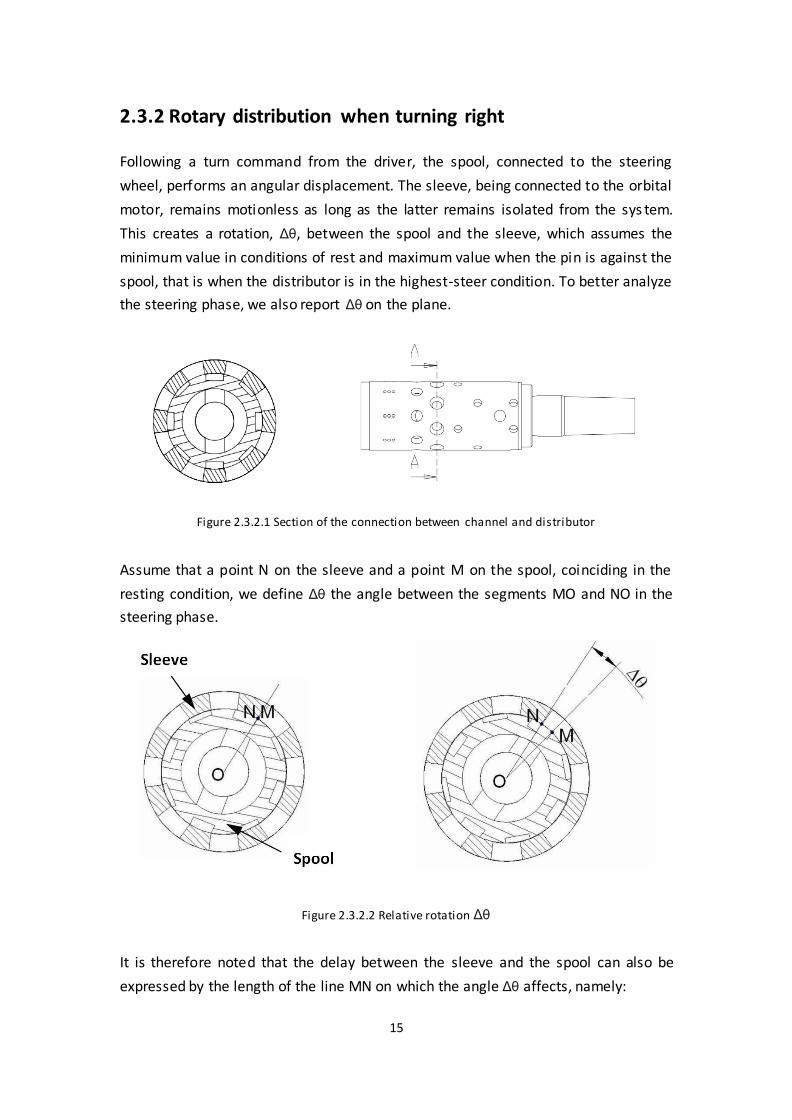
2.3.2 Rotary distribution when turning right

Following a turn command from the driver, the spool, connected to the steering

wheel, performs an angular displacement. The sleeve, being connected to the orbital

motor, remains motionless as long as the latter remains isolated from the sys tem.

This creates a rotation, Δθ, between the spool and the sleeve, which assumes the

minimum value in conditions of rest and maximum value when the pin is against the

spool, that is when the distributor is in the highest-steer condition. To better analyze

the steering phase, we also report Δθ on the plane.

Figure 2.3.2.1 Section of the connection between channel and distributor

Assume that a point N on the sleeve and a point M on the spool, coinciding in the

resting condition, we define Δθ the angle between the segments MO and NO in the

steering phase.

Figure 2.3.2.2 Relative rotation Δθ

It is therefore noted that the delay between the sleeve and the spool can also be

expressed by the length of the line MN on which the angle Δθ affects, namely:

16

MN=R·Δθ

where R indicates the radius of the coupling surface, equal to 12.5 mm. (Radius of

the spool).

Returning Δθ to the plane transforms the radial delay of the sleeve into a translation

of the spool, perpendicular to the axis of the same and equal to the length of the line

MN. This simplification does not involve any loss of information, provided that the

thicknesses of the sleeve and of the spool are returned to the mating surface only. In

this way the sections of the radial holes and the width of the grooves in the spool are

kept constant.

Figure 2.3.2.3 Turning distributor right (Maximum rotation)

Figure 2.3.2.3 shows the areas of fluid passage in the turning phase to the right. As

can be seen in this figure, the translation of the spool generates connections which

are not present in the resting phase. The contact between the pin and the spool, that

is the condition of maximum steering, is obtained by moving the spool equal to 2.4

mm, which is equivalent to a rotation of 11°.Following a Δθ > 0°, the connection

between the GA and the E-port is choked up to total isolation of the E-port. This step

takes place gradually to avoid sudden changes in pressure.

Port E GA

Orbit motor Left and right

Reservoir

Pin

17

Figure 2.3.2.4 Port communication holes obstructed during the maximum turn to right

For the eight holes connecting the GA, during the turning phase, four of them are

partially superimposed on comb millings and four of them on axial millings of the

orbit motor chambers (see Fig. 2.3.2.3). The flow rate coming from the GA is thus

sent both to the comb millings and to the four axial millings indicated in Figure

2.3.2.4. By passing these four millings the fluid passes through the orbital motor

distributor and is sent to the orbital machine through appropriate channels obtained

in the casing.

The coupling between the internal and external wheel of the orbit generates five

chambers of variable volume. Of these five:

•Two, with increasing volume, (C1, C2) are connected to the admission of the

machine

•Two, with decreasing volume, are connected to the discharge of the same.

• The remainder allows to isolate the two environments

Figure 2.3.2.5 Section of the orbit motor

18

.

Figure 2.3.2.6 Rotary distributor and orbit motor in right turning position

During the rotation five channels connected to the chambers and the chambers were

switched role becoming respectively environment under isolation and discharge with

the opposite direction to that of rotation of the orbital motor. The increasing volume

of chambers, shown in green in figure 3.3.2.7 is put in rotation, the wheel within the

orbit, its motion gives a volume decreasing to the other two chambers shown in

purple.

Figure 2.3.2.7 Motor and ports connection in maximum right turning position

19

These two chambers, decreasing in volume, send fluid to the grooves of the spool

through appropriate radial holes in the sleeve. For these four millings, only two are

directly involved (as the exhaust chambers of the orbit engine are two) while the

others are affected by the pressure information transmitted by the circumferential

milling. In this way the radial forces of the spool are balanced. Finally, the fluid

discharged from the orbit motor passes through the connecting holes to the working

port R and through a circular milling in the casing it is directed towards the port itself.

The output of the actuator connected to this port is thus caused.

Figure 2.3.2.8 Port L and R connection in maximum right turning position

The return fluid from the cylinder returns to the distributor through port L and is

sent to discharge through the millings which meet the seat of the pin and the spring

pack, shown in blue in the figure below.

20

Figure 2.3.2.9 Port L and tank connection in maximum right turning position

These 4 grooves represent in fact a single channel, since the holes in the seats are

through and allow the fluid to penetrate into the inner cavity of the spool. The

presence of oil inside this cavity guarantees the lubrication of the toothed coupling

between the Cardan shaft and the internal wheel of the motor. Summing up, to a

possible rotation of the steering wheel are generated that put in common the GA

with the orbital motor, which begins to rotate in a direction to the steering. A flow

rate is then sent, proportional to the speed of rotation of the motor, to the chamber

in expansion of the cylinder. The sleeve, dragged by the orbital motor through the

Cardan shaft, follows the movement of the spool until the two are centered again.

Figure 2.3.2.10 Rotation of the Cardan shaft

Figure 2.3.2.11 shows the connection millings in turning right condition.

21

Figure 2.3.2.11 Connection mill ings in turning right phase

2.3.3 Rotary distribution when turning left

Turning to the left, similar connections are made inside the distributor, such as to

feed the actuator chamber that was previously unloaded and vice versa. Only some

camouflage holes are used as shown in figure 2.3.3.1

• The holes that were used to discharge the actuator chamber are now engaged

with the milling of the spool traversed by the exhaust fluid of the motor / pump

• The fluid that previously allowed the actuator chamber to be powered, now

discharge it.

• The orbital motor changes towards rotation, also because the sleeve must follow

the spool in the new direction of rotation

22

Figure 2.3.3.1 Connection mill ings in turning left phase

23

Chapter 3

Components

3.1 Assembly of steering unit

The steering unit consists of several parts:

Figure 3.1.1 Assembly of steering unit

24

Figure 3.1.1 shows that assembly of steering unit, the main parts are: rotary valve

consist of casing, spool, sleeve in assembly 2, orbit motor in assembly 17.

1-dust seal ring 2-housing spool and sleeve 3-ball 4-ball stop 5-shaft seal

7-bearing 10-ring 11-cross pin 12-set of springs 13-cardan shaft 14-spacer

15-O-ring 16-distributor plate 17-gearwheel with 27.4 diameter 18-O-ring

19-end cover 20-O-ring 23-special screw with 47.6 diameter 24-name plate

30-complete relief valve 31-spring for relief valve

Figure 3.1.2 Section view of steering unit

1-spool 2-bearing 3-safety valve 4-cardan shaft 5-sleeve 6-distributor plate

7-orbit motor/pump 8-shell of orbit motor/pump 9-end cover 10-fixing screw

11-spring package 12-pin 13-non return valve 14-shell of the body

The OSPM 80 PB is a steering system consisting of a rotating distributor with

continuous positioning, which is constituted by a sleeve and a spool (figure 3.1.1 and

3.1.2) and an orbital motor/pump. They are all housed in a special shell. The steering

wheel is connected to the distributor spool by means of a grooved coupling, and the

spool, in turn, is coupled to the sleeve by means of the leaf springs. The connection

between the spool and the pin is carried out by means of a hole with a greater

diameter than that of the pin; This creates a space that allows a rotation of the pin,

25

with respect to the axis of the hole, between plus and minus 11 °, this represents

the end stop (figure 3.1.3). Then we can have a relative angle between sleeve and

spool as different working condition what we want.

Figure 3.1.3 Spool

Figure 3.1.4 Spool and pin

Figure 3.1.4 Spool, pin and sleeve

26

The mobility of the pin makes possible a rotation between the spool and the sleeve

that generates a passing line, between the grooves of the spool and the radial holes

of the sleeve. In this way, the flow of fluid coming from the flow generating group to

the orbital motor and therefore to the steering actuator is regulated. The sleeve is

also connected to the orbital motor by means of a cardan shaft that has a fork, seat

with a pin yoke.

Figure 3.1.4 Cardan shaft

Through the groove of the pin and rounded tooth on the shaft, inner wheel of the

orbit motor and sleeve are coupled, which allows the transformation of the

planetary motion of the motor in rotary motion of the sleeve, thus realizing the

mechanical feedback signal on the rotary distributor.

Figure 3.1.5 Orbit motor assembly

External gear of the

orbit motor

Internal gear of the

orbit motor

27

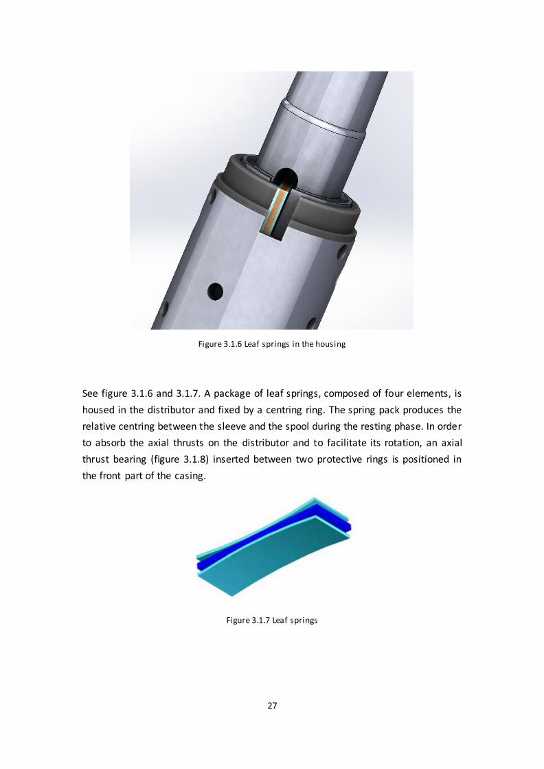
Figure 3.1.6 Leaf springs in the housing

See figure 3.1.6 and 3.1.7. A package of leaf springs, composed of four elements, is

housed in the distributor and fixed by a centring ring. The spring pack produces the

relative centring between the sleeve and the spool during the resting phase. In order

to absorb the axial thrusts on the distributor and to facilitate its rotation, an axial

thrust bearing (figure 3.1.8) inserted between two protective rings is positioned in

the front part of the casing.

Figure 3.1.7 Leaf springs

28

Figure 3.1.8 Axial thrust bearing and protective rings

The tank, the flow generating group, the L and R working ports, the motor/pump and

a further use port are connected to the casing, to which all the flow from the flow

generating group is addressed during the resting phase. These connections are

positioned circumferentially to the rotating distributor by means of special grooves.

Figure 3.1.9 Connects between ports and distributor spool

Figure 3.1.10 shows the sections of the spool for illustrating how the connections

between the Rotary distributor and the various working ports:

• With P the connection port to the GA

• With E to the external users

• With T the connection port to the reservoir

• With R and L the connecting ports to the chambers of the actuator cylinder

29

The five holes, with a smaller diameter than the ports previously indicated,

constitute instead the connections between the orbital motor and the rotating

distributor.

Figure 3.1.10 Section view of the connections

30

The tank, the flow generating group and the working ports are connected to the

casing by means of suitable holes which also act as a seat for the tightening screws.

Figure 3.1.11 Screws

3.2 Mechanical model

In order to build the simulation of the system, Simcenter Amesim can be used, it

offers us an integrated simulation platform to accurately predict the

multidisciplinary performance of intelligent systems. Simcenter Amesim enables us

to model, simulate and analyze multi-domain controlled systems and offers plant

modeling capabilities to connect to controls design helping you assess and validate

control strategies. At first we have to use Solidworks and ANSYS to define the

mechanical properties of the components. Torsional stiffness and virtual viscous

friction coefficient in Amesim are needed to simulate the mechanical model in

steering. Since the sleeve, from a mechanical point of view, is simulated by a spring

and damper.

The steering unit is integrated by the following main parts:

Sleeve

Spool

Cardan shaft

Springs

In the next we will analysis these parts one by one

31

3.2.1 Sleeve

The material of sleeve is AISI 1045 steel. AISI 1045 steel is a medium tensile steel

supplied in the black hot rolled or normalized condition. It has a tensile strength of

570 - 700 MPa and Brinell hardness ranging between 170 and 210. AISI 1045 steel is

characterized by good weldability, good machinability, and high strength and impact

properties in either the normalized or hot rolled condition.

Figure 3.2.1.1 Material of sleeve

Then we can get the moments of inertia from the model:

32

Figure 3.2.1.2 Inertia of the sleeve

Due to the pin joining, the moments of inertia should be the sum of the sleeve

inertia plus half of the pin’s inertia.

Pxsleeve=35437.25[g·mm²]=3.54·10-5[kg·m²]

Figure 3.2.1.3 Inertia of the pin

Pypin=431.20[g·mm²]=0.04·10-5[kg·m²]

So the total inertia of the sleeve is

Pxsleeve+ 1

2 Pypin=3.56·10-5[kg·m²]

33

In order to evaluate the stiffness and friction viscous we hypothesis that, in

maximum rotation, the pin contact with sleeve and spool, so the torque transferred

from pin is nearly equal to the torque on the steering wheel, is larger than the leaf

spring, we assume the parameters as follows: The fixed hinge is on the inner surface

in which the pin is located and the 3[N·m] torque is applied in the sleeve-pin contact

inner planes. Moreover on the surfaces between sleeve and springs we have

geometry fixed and there is 1[N·m] torque is applied by the springs. See figure

3.2.1.4.

Figure 3.2.1.4 Sleeve static test-Configurations

Solid-Works creates a mesh to perform the calculation via finite element method.

Figure 3.2.1.5 shows a summary of the mesh global parameters settings:

Figure 3.2.1.4 Sleeve static test-Mesh

34

Figure 3.2.1.5 and figure 3.2.1.6 represents the results of such test.

Figure 3.2.1.5 Sleeve static study-Von Mises tensions

Figure 3.2.1.6 Sleeve static study-Displacement

35

As the Von Mises tensions are in all parts of the body under the yield strength limit,

none of the deformations will be permanent and it is valid to assume that the piece

is behaving as a spring; therefore, being K[𝑁·𝑚

𝑑𝑒𝑔𝑟𝑒𝑒] the rigidity constant, γ[degree] the

maximum angular relative displacement (twist) and T[N·m],

the torque applied:

Ｋ·γ＝Ｔ

γ＝ｄ

r

where 'd' is the maximum displacement (perpendicular to the radius 'R') of the

sleeve. Being: d=7.76·10−5[mm], r=14.25[mm], then γ=5.45·10−6[rad].

If contact between pin and sleeve occurs, the equivalent torsion spring stiffness is:

Ksleeve=3[𝑁·𝑚]

5.45·10−6[rad]=5.51·105[N·m/rad]

or

Ksleeve=9601.32[N·m/degree]

The mechanical system can be simulated by a spring and damper, usual damping

values are around 5% to 10%.

Considering a Rotary Mass-Rotary Spring system of moment of inertia 'Ｉ', stiffness

'K' and viscous friction 'R', the motion law can be expressed as a second order

system:

Ｉ·�̈�＋Ｒ·�̇�＋Ｋ·θ＝０

or alternatively

�̈�+2·z·w0·�̇�+𝑤02·θ=0

where 'w0' is the natural pulsation and 'z' is the damping ratio, these values are

defined as:

w0=√𝐾

𝐼

z =𝑅

2·√𝐾·𝐼

Then if the value of damping equal to 5% is chosen for the present system, being:

I=3.56·10-5[kg·m²], Ksleeve=5.51·105[N·m/rad]

Rsleeve=2·0.05·√𝐾 · 𝐼=0.443[𝑁 ·𝑚

𝑟𝑎𝑑/𝑠]=0.046[

𝑁·𝑚

𝑟𝑒𝑣/𝑚𝑖𝑛]

36

In this case we assumed that the contact between pin and sleeve is totally rigid

because the stiffness K is big enough so the displacement can be ignored.

3.2.2 Spool

Now analyzing the spool it is also assumed that due to the pin joining , its inertia is

the sum of the spool plus half the pin’s inertia.

Figure 3.2.2.1 Inertia of the spool

Pxspool=18623.75[g·mm²]=1.86·10-5[kg·m²]

Pxspool+ 1

2 Pypin=1.88·10-5[kg·m²]

37

Then using the same finite element method we can simulate the stress and

displacement which is applied on the spool. See figure 3.2.2.2: Where the torque

received from the springs is 1 [N·m] , from the steering wheel on the shaft is 3[N·m],

from the pin is equal to the shaft but on opposite direction.

Figure 3.2.2.2 Spool static study-stress and displacement

The radius of the spool is 11[mm]. Following the results we can calculate:

d=1.20·10−3[mm], r=11[mm], then γ=1.17·10−4[rad].

So the torsion stiffness is:

Kspool=3[𝑁·𝑚]

1.17·10−4[rad]=2.56·104[N·m/rad]

or

Kspool=446.8[N·m/degree]

Considering the value of damping is equal to 5% then the viscous friction is:

Rspool=2·0.05·√𝐾 · 𝐼=0.069[𝑁 ·𝑚

𝑟𝑎𝑑/𝑠]=0.007[

𝑁·𝑚

𝑟𝑒𝑣/𝑚𝑖𝑛]

38

3.2.3 Cardan shaft

Cardan shaft is the connection between the pin and the inner gear of the orbit motor.

So when we talking about the mass moment of inertia we should consider not only

the shaft but also the orbit gear.

Figure 3.2.3.1 Inertia of the cardan shaft and orbit gear

Making the static analysis we can get:

Pxshaft=137.16[g·mm²]=1.37·10-7[kg·m²]

Pzgear=2156.79[g·mm²]=2.16·10-6[kg·m²]

39

Ptotal=Pxshaft+Pzgear=2.30·10-6[kg·m²]

Figure 3.2.3.2 Cardan shaft static study-stress and displacement

Then combine the geometry and simulation figure 3.2.3.2, we can get:

d=6.96·10−5[mm], r=5.5[mm], then γ=1.27·10−5[rad].

So the torsion stiffness is:

Kshaft=3[𝑁·𝑚]

1.27·10−5[rad]=2.36·105[N·m/rad]

or

Kshaft=4119.0[N·m/degree]

Considering the value of damping is equal to 5% then the viscous friction is:

Rshaft=2·0.05·√𝐾 · 𝐼=0.018[𝑁·𝑚

𝑟𝑎𝑑/𝑠]=0.0019[

𝑁·𝑚

𝑟𝑒𝑣/𝑚𝑖𝑛]

40

3.2.4 Springs

Spring is an elastic part between the sleeve and the spool. It provides the rebound

force to close the port when the driver hold the steering angle. So it is very

important for the system performance.

Spring is made of two couples of leaf springs inside a parallel steel board. When the

force acts on the board, it compresses the springs. So for this part, we simulate it

using ANSYS workbench.

At first we build the leaf spring model by measuring.

Figure 3.2.4.1 Leaf spring

Then we mesh the model by choosing a proper sizing as follows:

Figure 3.2.4.2 Leaf spring mesh property

Because when there is relative angle between sleeve and spool by leaf spring, the

counteract point is the contact point between housing of the spool and the spring.

We set the deformation of two points of the spring as follows: each side of the

deformation equals to 1mm.

41

Figure 3.2.4.3 Leaf spring deformation setting

After this we must set boundary constrains on the spring, we should make sure when

the displacement applied on the spring, the spring is fixed in the housing:

Figure 3.2.4.4 Leaf spring constrains

At last we can solve the model, see figure 3.2.4.5-3.2.4.8:

Figure 3.2.4.5 Leaf spring total deformation

42

Figure 3.2.4.6 Leaf spring equivalent stress

Then we have the reaction forces shows in figure 3.2.4.7, on the opposite end of side

on upper and lower spring, make up a torque on the spring.

Figure 3.2.4.7 Leaf spring reaction force

We assume that the displacement from 0 to 1mm in 1s. The value of the reaction

force is that:

Figure 3.2.4.8 Leaf spring reaction force parameter

43

From the geometry of the spring, length is 29.30mm, width is 6mm. Figure 3.2.4.9

shows that when the maximum angle is 11°, on each side of upper and lower plate

the rotation angle is 5.5°. And if we have 1mm deformation on the contact points

between spool and spring. In figure 3.2.4.9 we can have 2.12° rotation angle on

lower plate it means that we have 4.24° relative angle between sleeve and spool.

The spring width becomes 4.91mm.

Figure 3.2.4.9 Geometry of the compression spring

From the geometry and simulation , when the spring is compressed 1mm on point A

and B in figure 3.2.4.3, a force equals 2.79[N] acts on the end side of the spring in

figure 3.2.4.7, where the torque:

T=2.79[N]·(29.3-2.25)[mm] ·2=150.94[N·mm]

While from the geometry of the spring the compression is equal to 6-4.91=1.09[mm].

So we can get the stiffness of the rotary spring is:

K=150.94/1.09=138.48[N·mm/mm]

Then from the geometry relationship between sleeve and spool, we can get the

compression length x=(D- D−L·tan (α/2)

cos(α/2)) , where D is the width of the housing, L is the

spring length , α is the relative angel from -11° to 11°. Figure 3.2.4.10 represents the

relationship of the relative angel and the compression, we can consider it is a linear

function, ratio is:

β=x/α=2.83/11=0.257[mm/degree]

44

Figure 3.2.4.10 Function of the relative angle between sleeve and spool and compression

It means that when we have 1° relative angle of the sleeve and spool, the spring

compression is 0.257mm. Then we hypothesis the function of the spring is linear,

then the stiffness of the rotary spring is:

Krotary=K· β=35.6[N·mm/degree].

And when the spring is free, the width is 10.8mm, so the preload of the spring:

Fpreload=K·(10.8-D)=803.17[N·mm].

3.3 Amesim simulation connection

In order to simulate the hydraulic system performance, we should build the

mechanical part of the system first.

At previous we have finished the analysis of these important parts then we must

choose proper models for them in Amesim.

So we can build the mechanical system as follows:

mm

degree

45

Figure 3.3.1 Model of mechanical system

For sleeve and spool, ROTARY LOAD (for the inertia) with viscous friction

and a ROTARY SPRING (simulating the stiffness) are introduced.

Moment of inertia:

Pxsleeve+ 1

2 Pypin=3.56·10-5[kg·m²]

Pxspool+ 1

2 Pypin=1.88·10-5[kg·m²]

Viscous friction:

Rsleeve=0.046[𝑁·𝑚

𝑟𝑒𝑣/𝑚𝑖𝑛]

Rspool=0.007[𝑁·𝑚

𝑟𝑎𝑑/𝑠]

Rigidity stiffness of the sleeve:

46

Ksleeve=9601.32[N·m/degree]

Figure 3.3.2 Parameter of the sleeve and spool

For the leaf spring, we can use the ROTARY SPRING as well, but since the

compression of the leaf spring is equal to relative rotation between the sleeve and

spool, two ANGULAR DISPLACEMENT SENSORS are added in the two sides of

the leaf spring. This signal will be generated by the driver input signal through the

mechanical parts, then transferred to the hydraulic system.

From the previous analysis, the stiffness and the preload values are as follows:

Kspring=3.56·10−2[N·m/degree], Fspring=803.17[N·mm]

Figure 3.3.3 Parameter of the leaf spring

47

For the spool and sleeve interaction, the equivalent model is that of the elastic

double end-stop in rotary motion (in which the viscous friction is negligible

due to low relative angle velocities). This model allows both, upper and lower

connections, to rotate freely during a determined relative angle (∆α=11°), if that

value is exceeded the sum of the spring stiffness will now rule the relative motion,

nevertheless as the double end-stop’s inner stiffness is very big the spool and sleeve

will move practically solely. And this part is also used for mechanical connection

between driver and the wheel. When the hydraulic system is unavailable this

connection will take part in.

So the stiffness is the stiffness of the spool, as follows:

Figure 3.3.4 Parameter of the spool and sleeve interaction

For the steering column, we assume that the stiffness rigidity is:

Ksteering column= Kspool /10=44.68[N·m]

which represents the connection stiffness between steering wheel and the spool. In

Amesim it can be indicated by ROTARY SPRING .

For the Cardan shaft and orbit gear, ROTARY LOAD can be used, where:

Kshaft=4119.0[N·m/degree], Rshaft=0.0019[𝑁·𝑚

𝑟𝑒𝑣/𝑚𝑖𝑛].

48

Chapter 4

Simulation of the system

4.1 Amesim submodel selection and governing equations

Each one of the Amesim models selected for the several parts of the steering system

has in turn a few submodel associated. In the following subsections the selection of

each particular submodels is explained and ruling equation of each one of them.

4.1.1 Variation area of the distributor orifices

From the beginning of the simulation, we should calculate the variation area of the

distributor orifices when the system is under working condition.

We can simplify the model to analyse the fluid flow as follows:

Figure 4.1.1.1 Simplified model of the steering unit

49

In this case the fluid flows which are discharged to each ports are decided by the

opening areas of the orifices. And the opening areas are decided by the relative

angle between sleeve and spool as figure 4.1.1.2 and figure 4.1.1.3:

Figure 4.1.1.2 Sketch areas on the sleeve and spool on centre position

Figure 4.1.1.3 Sketch areas on the sleeve and spool when turning right

• A1 is the overlapping area between orbit motor and port R

• A2 is the overlapping area between orbit motor and GA

• A3 is the overlapping area between port R and left chamber of the actuator

• A4 is the overlapping area between port L and right chamber of the actuator

• Ag is the overlapping area between GA and steering unit

50

• At is the overlapping area between port L and reservoir

• Ae and Ae1 are the overlapping areas between GA and port E

In the case of turning right, the fluid is discharged by the GA to orifices Ag, through

the orifice A2 to the orbit motor, then discharged by the orbit motor to orifices A1

and A3, fill into the left chamber of the actuator, then push the piston to right. On

the other side of the actuator, fluid flows through A4 and At, back into the reservoir.

For port E, we can observe that when the system is moving from the centre position

to the right position, the holes Ae and Ae1 are closed gradually.

Then using the mathematical method, the variation of the relative angle and the

area of holes can be calculated as follows:

Figure 4.1.1.4 Variation of the relative angle[°] and area of orifices[mm2]

Figure 4.1.1.5 Variation of the relative angle[°] and area of orifices[mm2]

0,0000

20,0000

40,0000

60,0000

80,0000

100,0000

120,0000

140,0000

160,0000

180,0000

1 2 3 4 5 6 7 8 9 10 11 12

Variation of the distributor area

SA1 SA2 SA3 SA4 SAt SAg SAe SAe1

51

From the figure 4.1.1.4 and figure 4.1.1.5 we can see when the relative angle

increasing, the area of the steering orifices increasing, port E which is connected to

the external equipment, is closed gradually. On the other hand, when the steering

unit is on the centre position, the resting phase, fluid from GA is totally discharged to

the external equipment through port E.

In order to simulate the variation area of the orifices in Amesim, we can use the

block VOR002 - variable hydraulic orifice with tables or equations

hd=f(x) and a=f(x). Then we can set the variation area of the orifices as a function of

relative angle.

4.1.2 Ideal orbit motor/pump

Then the block HYDFPM01 - fixed displacement hydraulic pump or motor with

tabulated efficiencies f(dp, w, (T)).

The theoretical flow rate of a hydraulic machine, either pump or motor, is defined as:

QTh=V×w. Where V is the displaced volume (corresponding to the user parameter

displacement) and w is the shaft speed.

The theoretical torque, either for a pump or for a motor, is defined as: TTh=V×dp .

Where dp = p2-p1 is the differential pressure at the hydraulic ports of the hydraulic

machine.

The real quantities are then derived by the theoretical ones through efficiencies.In a

real displacement machine several energy losses occur, mainly divided in two

categories: Volumetric losses, determined by internal and external flow leakages

through different gaps or clearances, flow losses due to the fluid compressibility.

Hydraulic mechanical losses, representing torque losses due to dry and viscous

friction between moving elements.

Due to volumetric losses, the real flow rate delivered by a displacement pump is

consequently less than the theoretical value generated by an ideal pump (with the

same shaft speed). While in the case of a displacement motor, the required inlet

flow rate is greater than the theoretical value needed by an ideal motor.

Due to the hydraulic mechanical losses, the torque required by a displacement pump

with a certain differential pressure is greater than the ideal value. While in the case

of a displacement motor, the differential pressure applied to the hydraulic machine

52

must be greater than the theoretical value (to produce the same torque).

Depending on the pump or motor working mode, the real flow rate and torque are

evaluated as follows:

Figure 4.1.2.1 Definition of efficiencies, for pump or motor.

Using this block we can simulate both pump and motor, which corresponds to

changing the sign of the flow rate and torque depending on dp and w:

Figure 4.1.2.2 Definition of efficiencies, for pump or motor.

53

4.1.3 Double acting steering cylinder

Double acting steering cylinder can be used for this system. With rod diameter

d=25[mm] and piston diameter D=50[mm]. In our design, the maximum number of

steering wheel revolution is=3, steering unit displacement (orbit motor) V=80[cc],

which means that the maximum volume by actuator from middle to lock is

Vmax=240[cc]. Area in chamber:

A=𝜋(𝐷2−𝑑2 )

4=1472.6[mm2]

so the actuator stroke:

L=Vmax/A=163[mm]

For the vehicle the maximum steering angle is 36°, so the offset between steering

rod and drive shaft (figure 4.1.3.1):

a=)tan(36

L

=224.2[mm]

The maximum pressure from the steering system (relief valve pressure) Pmax=80[bar],

so the maximum actuator force:

Fmax=Pmax·A=11780.8[N]

maximum steering torque :

Tmax=Fmax·a=2641.3[N·M]

Figure 4.1.3.1 Double acting steering cylinder

offset

54

In Amesim HJ021 - double hydraulic chamber double rod jack with no

orifices at flow ports can be used to simulate our double acting steering cylinder.

4.1.4 Hydraulic chambers

There are several volumes that are considered in the hydraulic model. In Amesim we

can use HC00 - simple hydraulic chamber to simulate the hydraulic chamber

with a constant volume and pressure dynamics. Each port receives a flow rate as

inputs and gives a pressure as output. They are used to compute the time derivative

of pressure.

Figure 4.1.4.1 Chambers between sleeve and spool

The basic formula used for computing the derivative of pressure in terms of the net

flow rate and total volume is Dp/dt=B(p1)(q1+q2)/vol0, where B is the bulk modulus.

Sum of flow rates entering into the volume, qsum=q1+q2

55

4.1.5 Hydraulic tank

In this simulation, we assume that ideal fluid hydraulic tanks what we need. So in

Amesim TK000 - tank modeled as constant pressure source can be used.

4.1.6 Resistance load

Resistance by steering is coming from the friction force between wheels and road.

Moreover it has two endstops in the steering cylinder. In Amesim MAS005 -

mass with friction and ideal end stops can be used.

MAS005 represents the one-dimensional motion of a two ports mass under the

action of two external forces in N and frictional forces. The submodel returns the

velocity in m/s, the displacement in m and the acceleration of the mass in m/s 2. The

displacement is limited to a specified range by inclusion of ideal end stops.

Use MAS005 for linear motion of a mass with two forces applied to it when there is

friction and restrictions on displacement with no elastic effects during contact.

Figure 4.1.6.1 Resistance load connections

Figure 4.1.6.1 shows that the assembly of the resistance load. We can see that the

force is acted on the right through MAS005 to the actuator. Then the force

generated by the hydraulic system to the actuator should be equal to the input

resistance force.

56

4.2 Simplified model of the hydraulic system

Figure 4.2 Simplified model of the steering system

Res

ista

nce

load

Hyd

rau

lic p

art

Lo

gic

cont

rol p

art

Mec

hani

cal p

art

57

Figure 4.2 shows that the simplified model of the steering system. It consists of three

parts: mechanical components, hydraulic components and resistance load

components. In following sections we will explain respectively.

4.2.1 Mechanical parts

From figure 2.3.1, we have built the model of mechanical parts. In the assembly of

the whole system, it represents the connection between driver input and hydraulic

system.

Figure 4.2.1.1 Signal input and output in the mechanical system

Signal 1 is the input signal from the driver, which is the function of steering wheel

angle and time. It means that in our simulation, the reaction of the steering angle of

the wheel should be proportional to the angle of the steering wheel.

Signal 2 is the angle of the sleeve and spool, then we can get the relative angle

between sleeve and spool, which decides the variation area of the orifices between

sleeve and spool. The signal will be sent to the logic control of the area variation

orifeces in the hydraulic parts (figure 4.2).

58

Signal 3 is the input of the mechanical system which is from the ideal orbit motor in

hydraulic parts. It means that the orbit motor drives Cardanshaft, then the sleeve

rotates with the orbit motor.

4.2.2 Hydraulic components

Figure 4.2.2.1 Signal and logic control in the hydraulic system

Hydraulic part is the core part of the steering system. It connects mechanical part

and resistance part. Then main purpose is that reduces the force acting on the

steering wheel. Signal 2 and signal 3 have been explained before, signal 4 is the

output piston force of the actuator. Which counteracts the resistance force.

In order to simulate the operation of the system correctly. We set three parts of the

logic control under signal 2.

In figure 4.2.2.1, upper part controls the area variation of orifices which are related

to steer right. It means that when the driver wants to turn right, this part received

relative angle of the sleeve and spool from signal 2, sent to the variable orifices.

Signal 2

Signal 3 Signal 4

Lower part

Middle part

Upper part

Relief valve

Non-return

valve

59

Then the fluid is allowed to passing through the opened orifices, fil ling left chamber

of the actuator,pushing piston to right. Fluid in right chamber can be discharged to

the tank. At the same time middle part controls turning left so it should be closed.

Lower part represents the variation area of the port E which connects the external

devices.

Figure 4.2.2.2 Fluid flow when turning right

Figure 4.2.2.2 shows the fluid flow when turning right clearly, the variable orifices

VAR002 correspond to the orifices in figure 4.1.1.1 respectively. Fluid generated by

the pump, passing through orifices to the left chamber of the actuator. While the

upper logic control part controls the area of the orifices.

On the contrary, turning left is controlled by middle part of the logic control. It is

similar as turning right.

Relief valve in figure 4.2.2.1 is used to prevent the system when resistance force is

very large, increased pressure could damage the system, it is set to be 80[bar]. So

when the pressure from the pump is larger than 80[bar], through this valve, fluid can

A1

Ag

A2

A4

A3

At

Ae Ae1

60

flow back to tank. Non-return valve in figure 4.2.2.1 is used to supply fluid from tank

when the pump is lack of fluid. Prevent cavitation in the channel.

4.2.3 Resistance part

Figure 4.2.3.1 Resistance part

This part has explained before, we just need to make sure the resistance force input

sign is equal to the steering wheel input, making sure that the resistance load is

usually resisting the force from the piston rod.

4.2.4 Simulation and analysis

At first we should check the correction of the model. Then we set three sets of

parameter input, as follows:

Figure 4.2.4.1 Steering input signal[Degree]

61

Figure 4.2.4.2 Steering input signal speed[Degree/s]

It shows that the driver input steering angle signal as a cycle of time. Then from the

output signal of the actuator we can get the displacement of the piston and wheel

angle as follows:

Figure 4.2.4.3 Piston displacement (left) and wheel steering angle (right)

The simulation shows that the output signal is proportional to the input signal, but if

we compare the curve between input and output one by one we can find the

difference as follows:

62

Figure 4.2.4.4 Comparison between input degree and output displacement of piston

Figure 4.2.4.5 Details comparison between input degree and output displacement of piston

63

We can see that at every cornering of the steering input, we have hysteresis acting

on the actuator. One of the reason is that the spring between sleeve and spool,

which corresponds to the function of servo system. It means that when we hold the

steering wheel not rotating, the orifices should be closed. Under this condition, spool

is not rotating by our hands, compressed spring release the force to the sleeve and

spool, then the sleeve back to centre position, with relative angle between sleeve

and spool is decreasing. But during the spring is compressing or sketching, it needs

time to open or close the orifices, so there is a reason why we have delay.

We can see more details for the relative angle between sleeve and spool:

Figure 4.2.4.6 Relative angle between sleeve and spool

We can see that the spring closed the orifices slowly, we also can find there are

vibrations when we start steering. This is caused by impact and friction between

mechanical parts and vibration of the spring, after few millisecond it becomes stable.

When the steering speed is faster in figure 4.2.4.2, relative angle is larger,

compression force acting on the spring is larger. It means that opening area of

orifices becomes larger, we need more flow rate to push the piston to steer and

more torque should be put on the steering wheel, to compress the spring more

between sleeve and spool. Figure 4.2.4.6 shows that increasing the relative angle

with increasing the steering speed. Figure 4.2.4.7 as follows shows the flow rate in

the actuator and torque we need on the steering wheel.

Time for spring expansion

64

Figure 4.2.4.7 Steering speed effects the flow rate and torque

Under the design of OSPM PB, the port E should be closed gradually with the

increasing of relative angle. Figure 4.2.4.8 shows that the flow rate in port E, when

we steer the vehicle, fluid flow in port E is decreased, and more fluid flow we need

to steer, less fluid is discharged to port E, through the decreased area of orifices. It

means that the steering system operation has high priority than the external devices.

Figure 4.2.4.8 Flow rate in port E (Ae on the left and Ae1 on the right)

Figure 4.2.4.9 shows that actuator force is equal to resistance load regardless of

speed variation. It also can be evaluated by the difference pressure in each chamber

of the steering cylinder multiply the chamber area as we will talk as follows.

Figure 4.2.4.9 Actuator force (left) and resistance load (right)

65

Figure 4.2.4.10 Pressure at left chamber and right chamber with different steering speed

Figure 4.2.4.10 shows that the pressure at left chamber and right chamber. At first

we can evaluate the force output from the rod. For example the yellow line on 0-2

second, we can read that we have 51.75[bar] at left chamber and 17.8[bar] at right

chamber, chamber area comes from our design A=1472.6[mm2]. So the force is:

F=(Pleft-Pright)·A=(5.175-1.78)[Mpa] ·1472.6[mm2]=4999[N]

It is the same as the value in figure 4.2.4.9. The difference of the pressure between

left and right chamber is decided by load.

From Bernoulli equation: “In most flows of liquids, and of gases at low Mach

number, the density of a fluid parcel can be considered to be constant, regardless of

pressure variations in the flow. Therefore, the fluid can be considered to be

incompressible and these flows are called incompressible flows. Bernoulli performed

his experiments on liquids, so his equation in its original form is valid only for

incompressible flow. A common form of Bernoulli's equation, valid at any arbitrary

point along a streamline” is:

Where:

v is the fluid flow speed at a point on a streamline,

g is the acceleration due to gravity,

z is the elevation of the point above a reference plane, with the positive z-direction

pointing upward – so in the direction opposite to the gravitational acceleration,

66

p is the pressure at the chosen point, and

𝜌 is the density of the fluid at all points in the fluid.

The constant on the right-hand side of the equation depends only on the streamline

chosen, whereas v, z and p depend on the particular point on that streamline.

The following assumptions must be met for this Bernoulli equation to apply:

The flow must be steady, i.e. the fluid properties (velocity, density, etc...) at a point

cannot change with time,

The flow must be incompressible – even though pressure varies, the density must

remain constant along a streamline;

Friction by viscous forces has to be negligible.

When the fluid through orifices, we have loss of pressure, transfer the Bernoulli

equation we can get :

Q=Ce·A·√2·(𝑃1−𝑃2)

𝜌

Where Q is the flow rate through the orifice, Ce is orifice flow coefficient, A is orifice

area, P1 and P2 is each side pressure of the orifice, 𝜌 is density of the fluid.

Then we can choose an orifice randomly for example. Orifice A3 in first 0-2 second.

67

Figure 4.2.4.11 Orifice A3 loss pressure in 0-2 second

From the figure 4.2.4.11, in first 0-2 second, Ce=0.48, A=2.72[mm2], P1=3.69[Mpa],

P2=3.62[Mpa], then Q=0.48·2.72·10-6·√2·(369000 −3620000 )

850=16.75·10-6[m3/s], it is the

same as the last plot in figure 4.2.4.12. So we can say in our simulation the orifice

works correctly.

For orbit motor/pump, Q=q·n, Q is fluid flow rate generated by the pump, q is the

displacement of the orbit motor and q=80[cc/rev] in our case, n is rotating speed.

Figure 4.2.4.13 Orbit motor/pump behavoir on 1.5s

From figure 4.2.4.13 we can find that efficiency is 100%, n=12.5[rev/min], then

Q=80·12.5=1000[cc/min]=1[L/min], the value is equal to the simulation.

68

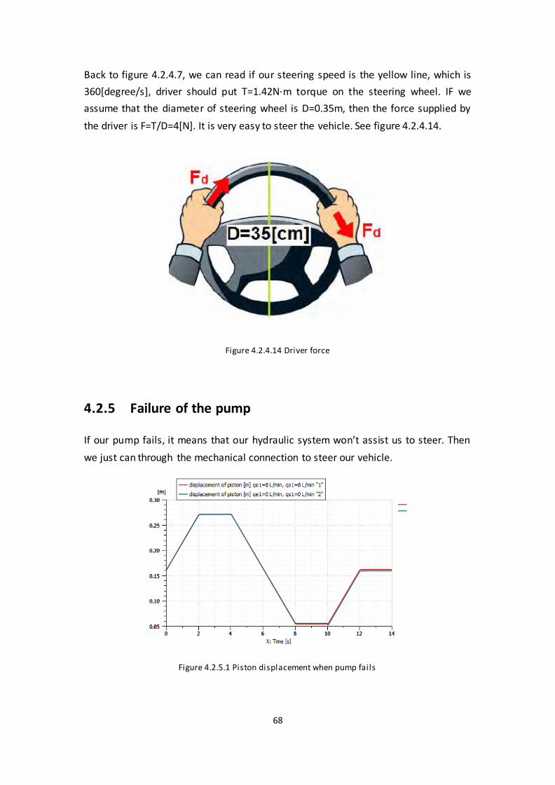
Back to figure 4.2.4.7, we can read if our steering speed is the yellow line, which is

360[degree/s], driver should put T=1.42N·m torque on the steering wheel. IF we

assume that the diameter of steering wheel is D=0.35m, then the force supplied by

the driver is F=T/D=4[N]. It is very easy to steer the vehicle. See figure 4.2.4.14.

Figure 4.2.4.14 Driver force

4.2.5 Failure of the pump

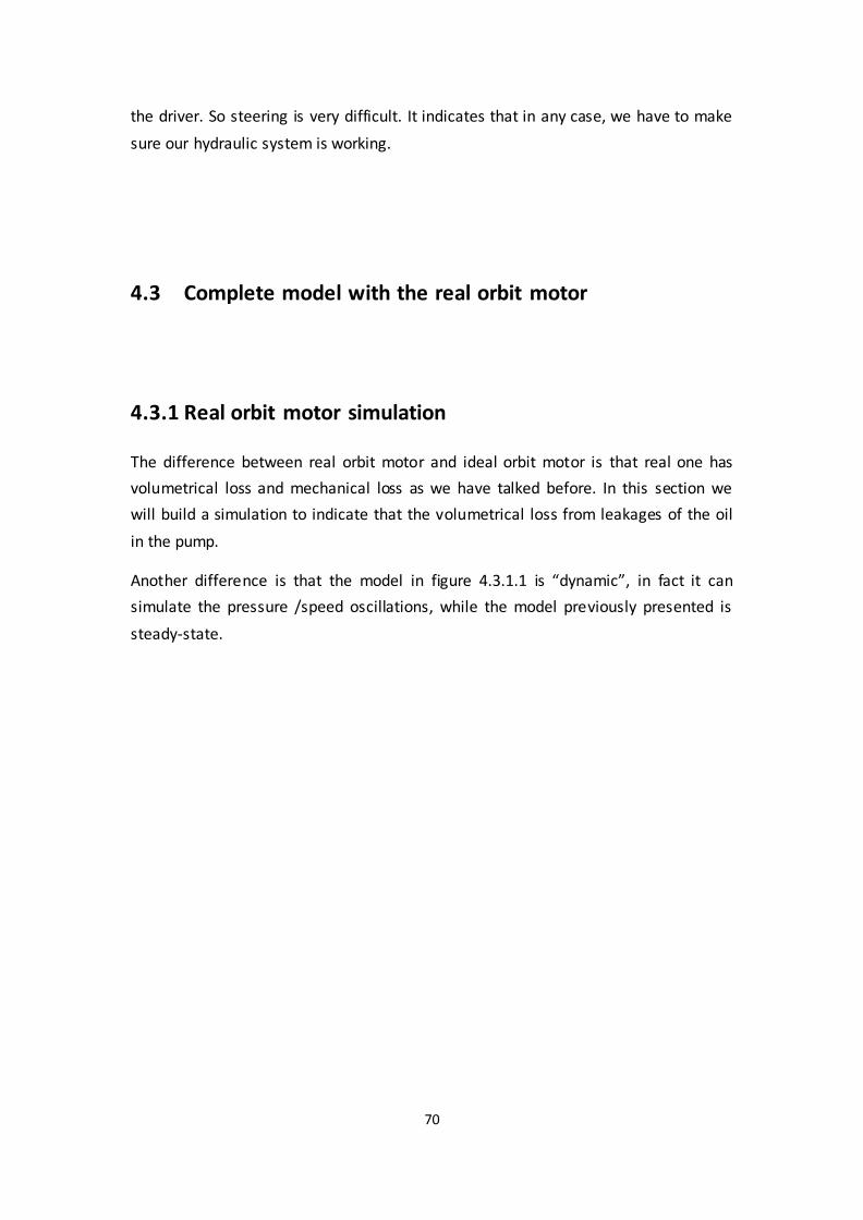
If our pump fails, it means that our hydraulic system won’t assist us to steer. Then

we just can through the mechanical connection to steer our vehicle.

Figure 4.2.5.1 Piston displacement when pump fails

69

From figure 4.2.5.1, the displacement of piston is almost the same as the normal

condition. The reason is that when the pump fails, we rotates the steering wheel

then the spool is rotating, when the relative angle is 11° which is maximum relative

angle between spool and sleeve, the pin fixed in the sleeve will contact with spool,

then sleeve is rotated with the spool. Orbit pump connected to the sleeve by Cardan

shaft and pin, is then rotated. Fluid oil sucked by orbit pump is delivered to the

steering cylinder, then the vehicle is steered. We can see in figure 4.2.5.2, the blue

line represents when pump fails, the relative angle reached 11° between spool and

sleeve, is different from in normal condition, the red line.

Figure 4.2.5.2 Relative angle between sleeve and spool when pump is failure

Figure 4.2.5.3 Driver torque when pump is failure

Figure 4.2.5.3 shows that when there is no fluid generated by the pump, driver

should supply a much bigger torque than normal case on steering wheel. For now

T=55N·m, in our prevouis hypothesis, diameter D=0.35m, then F=55/0.35=157[N] by

70

the driver. So steering is very difficult. It indicates that in any case, we have to make

sure our hydraulic system is working.

4.3 Complete model with the real orbit motor

4.3.1 Real orbit motor simulation

The difference between real orbit motor and ideal orbit motor is that real one has

volumetrical loss and mechanical loss as we have talked before. In this section we

will build a simulation to indicate that the volumetrical loss from leakages of the oil

in the pump.

Another difference is that the model in figure 4.3.1.1 is “dynamic”, in fact it can

simulate the pressure /speed oscillations, while the model previously presented is

steady-state.

71

Figure 4.3.1.1 Real orbit motor model

In order to simulate orbit motor, we need to simplify the operation process of the

orbit motor. The flow volume in a chamber is variation with the relative angular

position between internal and external gear. It means that with the rotation of

internal gear, volume in each chamber is changing. Volume in each chamber is from

close to open then to close in 1/(N-1)=0.25 revolution of the shaft. In our orbit motor,

it has 5 chambers. Every adjacent chamber has a phase shift which is 2π/5 degree. In

this case, we can build a model is that fluid generated by pump passes through each

chamber with variation area of orifices, and with leakages, sent to the outlet of the

motor. Then the fluid flow drives the internal gear rotation, with a torque to the

shaft. On the other side of shaft, we add a resistance torque. We can see more

details in figure 4.3.1.2:

72

Figure 4.3.1.2 Details of real orbit motor model

73

From the equation M·w=Q·p, where M is the torque delivered by a chamber, w is the

rotary speed of the shaft, Q is the flow rate, p is the outlet pressure of the chamber.

Then M· 𝑑𝜃

𝑑𝑡=

𝑑𝑉

𝑑𝑡·p, so M=p·

𝑑𝑉

𝑑𝜃. Torque delivered by the motor is the overlaid value

from the torque delivered by each chamber, then we add torques from five

chambers is the torque which is acted on the shaft.

Figure 4.3.1.3 Leakages of chamber

In order to simulate leakages between internal and external gear, we can transfer

this leakage to which between a cylinder spool or piston and cylinder sleeve, as well

as the corresponding viscous friction force, using the Amesim model BAP11-piston

and model BAF01-leakage with variable length, eccentricity and viscous friction in

figure 4.3.1.3.

Figure 4.3.1.4 Angular velocity of the shaft (left) and output flow rate from motor (right)

Piston

Leakage

74

From figure 4.3.1.4, angular velocity of the shaft mean value n≈100[rev/min], and

the displacement of our orbit motor v=80[cc/rev], from the equation:

Q=n·v=100·80=8000[cc/min]=8[L/min]

The value is the same as our simulation in figure 4.3.1.4.

In the motor, efficiency is equal to useful power of the shaft divided by the expended

power from the fluid. In this case, useful power Puse= M·w, see figure 4.3.1.5, we can

get: Puse=1[N·m] ·10.64[rad/s]=10.64[W].

Figure 4.3.1.5 torque on the shaft (left) and rotary velocity of the shaft (right)

Expended power Pexp=(Pin-Pout) ·Q. Pin and Pout is the inlet and outlet pressure of orbit

motor, Q is the flow rate, and is equal to 8[L/min] from the pump. See figure 4.3.1.6,

Pexp=(Pin-Pout) ·Q=(0.415-0.304)[Mpa] ·8[L/min]/60=0.0148[Kw]=14.8[W]

Figure 4.3.1.6 Pressure at motor inlet (left) and at motor outlet (right)

75

So the efficiency η= Puse/ Pexp=71.9%. It is worth noting that this value is just an

sample of calculation. The losses depend on the value of clearance and friction,

which are quite random in the model.

4.3.2 Real orbit motor inside the steering system

Finally we combine the real orbit motor model and the steering system, instead the

ideal one. The torque signal comes from the mechanical system connects the orbit

motor shaft, and the fluid flow signals connect inlet and outlet port of orbit motor.

76

Figure 4.3.2.1 Real orbit motor connection

Real orbit motor

77

Figure 4.3.2.1 shows real orbit motor in hydraulic system, the icon “real orbit motor”

represents the real orbit motor model in previous section.

Then we can see figure 4.3.2.2, the input steering wheel angle signal is proportional

to the output displacement of the actuator piston and the wheel steering angle. It

means that our simulation is correct.

Figure 4.3.2.2 Real orbit motor in the steering system

If we compare real case and ideal case, figure 4.3.2.3, red line represents piston

displacement in the system with ideal orbit motor, and blue line represents the

system with real orbit motor. The real curve is not good as the ideal one, it has

vibrations. We can find in real case the piston movement is lower than the ideal one,

this is because of the leagakes in the orbit motor. The real orbit motor efficiency is

not 100% anymore. The leakages also effect the feedback of the rotary valve. It

produces vibration on relative angle (figure 4.3.2.4), it means that the vibration is

acted on the leaf springs and fluid flow through rotary valve is not constant.

Figure 4.3.2.3 Piston displacement in ideal case and real case

78

Figure 4.3.2.4 Relative angle in ideal case and real case

In conclusion, avoid leakages in the orbit motor can increase the stability of the

steering system. Also can increase the handling behavior of the steering.

79

Chapter 5

Conclusion

During the study in Fluid Power Research Laboratory Politecnico. We measured the

geometry of “OSPM 80PB” mini hydraulic steering unit. And then we built FEM

model to analyze the mechanical properties by Solidworks and Ansys. Finally we built

the hydraulic model and analyzed the hydraulic properties by Amesim. Since the

models and analyses are simple, further more we can change parameters of each

part which can increase the performance of the steering unit, such as viscous

damping coefficient corresponding the vibration of the system. What’s more, the

offset between ideal case and real case can be decreased by simulation.

Nowadays, the newest hydraulic steering unit is under electronic control, which can

increase the reaction speed and accuracy. But it is much more expensive than the

traditional one.

80

Reference

1. Nicola Narvegna, Massimo Rundo, 2010. Automotive Fluid Power Systems,

Politeko, Torino, 2010.

2. SAUER DANFOSS, 2010. Mini Steering Units, Technical Information; General

Steering Components, Technical Information; OSPB OSPM [Online] Available at:

<http://www.sauer-danfoss.com/Products/Steering/HydraulicSteeringUnits/OSP

M/index.htm>

3. Genta Giancarlo, Morello Lorenzo, 2009. The Automotive Chasis. Volume I and II,

Springer, 2009.

4. Ambrosino Gaston Omar, 2013. Simulation And Analysis Of Hydraulic Steering

Systems For A City Car Prototype.

5. Giovanni Cala, 2007. Unita’ Di Sterzatura Idrostatica: CAD 3D, Schema

Simbologico E Analisi Di Una Idroguida.

6. Contents Of Hydraulic Library Of The AMESim Design Exploration Manual.