Embed Size (px)
Citation preview
Politecnico di Milano
School of Industrial and Information Engineering
Master of Science in Mechanical Engineering
PRELIMINARY DESIGN AND AERODYNAMICPERFORMANCE EVALUATION OF MULTI-STAGE
CENTRIFUGAL COMPRESSORS
Advisor: Prof. Paolo Gaetani
Co-Advisor: Dr. Sergio Lavagnoli
Candidate:
Andrea Cappelletti - Matr. 853746
Academic Year 2016-2017

Ringraziamenti
Ringrazio il Prof. Gaetani per avermi offerto l’opportunita di parteciparea questa nuova esperienza. Un grazie anche a Sergio per avermi seguito davicino lungo questo percorso e a Zuheyr per il caloroso sostegno. Ringrazioovviamente Alessandro per avermi offerto la sua supervisione e i suoi consiglidurante tutto il progetto.
Un ringraziamento speciale va alla mia famiglia, che ho sempre sentitoaccanto nonostante la lontananza.
Ringrazio infine le tante persone che al Von Karman hanno contribuito arendere speciale questa esperienza.
i

Abstract
The present Master Thesis deals with the implementation of a program forthe preliminary design and performance evaluation of multi-stage centrifugalcompressors. In this regard, a research work has been previously success-fully developed by the former student of Polytechnic of Milan AlessandroRomei, leading to an automatic MatlabR© program, called CCD (CentrifugalCompressor Design). CCD allows to generate an initial sizing of the ma-chine requiring only few input parameters such as the mass flow, the suctionconditions, the fluid properties and the total pressure ratio. Nonetheless,since in CCD the performances of the compressor are considered to dependupon global parameters, as the flow coefficient and the peripheral Mach num-ber, the need of a more precise approach was felt, so to search for a bettercapturing of the real behavior of the machine. Proceeding from this basis,the present project is targeting the implementation of a numerical designmethodology based on modern 1D loss correlations, that can guarantee agood performance prediction at the operating point, to model the principalcomponents of multi-stage centrifugal compressors: the impeller, the vanedand vaneless diffuser, the return system and the final volute.
Successively, the computation of the efficiency and pressure ratio mapsof the compressor has been carried out adapting the existing off-design pro-cedure created by Casey and Robinson (2013) and developed by Al-Busaidiand Pilidis (2016).
Finally, four test cases, representative of different kinds of compressors,have been accounted to apply and validate the code comparing the predic-tions of the main geometrical and thermodynamic quantities with referencedata and with the results of the previous version of CCD.
iii

Sommario
Il compressore centrifugo rappresenta una delle macchine a fluido maggior-mente versatili, svariando da applicazioni per impianti di trattamento chim-ico fino a sistemi di refrigerazione e propulsione dei veicoli, grazie ad unabuona compattezza e alle elevate prestazioni che e in grado di garantire,sia in configurazioni monostadio sia multistadio. Inoltre, grande interesse esuscitato dai margini di miglioramento di cui ancora dispone, essendo parti-colarmente complessi da studiare e comprendere a fondo i meccanismi fluido-dinamici che avvengono al suo interno, anche se grandi sforzi computazionalivengono compiuti a riguardo. Per tali motivi, la fase di progettazione diventamolto delicata e strumenti di supporto al lavoro degli ingegneri possono riv-elarsi molto utili per indirizzare correttamente i successivi studi. In questocontesto si inserisce la presente Tesi Magistrale, svolta presso il Von KarmanInstitute for Fluid Dynamics (VKI) dove si era precedentemente effettuatauna collaborazione con un ex studente del Politecnico di Milano, AlessandroRomei, che aveva portato alla creazione di un software MatlabR©, chiam-ato Centrifugal Compressor Design (CCD), per la progettazione preliminaredi compressori centrifughi. In breve, ricevendo in un input file i principaliparametri di progetto, quali portata, condizioni termodinamiche in ingresso,rapporto di compressione totale e proprieta del fluido di lavoro, CCD gen-era un dimensionamento di massima della macchina calcolando le principaligrandezze geometriche e stima l’efficienza del compressore utilizzando un ap-proccio a parametri globali, tra cui il coefficiente di portata e il numero diMach.
L’obiettivo di questo lavoro e lo sviluppo e l’implementazione di unametodologia che tenga invece conto, dal punto di vista uno-dimensionale,delle specifiche perdite aerodinamiche che si generano all’interno del compres-sore per calcolare le prestazioni nel punto di funzionamento e dimensionaredi conseguenza i suoi principali componenti: la girante, il diffusore palet-tato e non palettato, il sistema di ritorno e la voluta. Piu nel dettaglio, leperdite degli elementi non palettati saranno valutate attraverso equazioni diconservazione del momento angolare e di conservazione dell’energia, mentre
v
vi
per gli altri componenti verranno considerati specifici coefficienti di perditadi pressione totale.
Una volta terminata la parte di design, il programma genera, con unaroutine preesistente basata sui lavori di Casey e Robinson (2013) e Al-Busaidie Pilidis (2016), le mappe di efficienza e rapporto di compressione fuori dallacondizione di progetto.
Infine, quattro casi verranno utilizzati per l’applicazione e la validazionedella nuova metodologia, considerando macchine molto diverse tra loro: uncompressore a tre stadi con interrefrigeratori, un cinque stadi funzionante conuna miscela di idrocarburi, un sei stadi adibito alla compressione di idrogenoe lo stadio finale di un compressore assi-centrifugo per uso propulsivo. Ilconfronto sara realizzato comparando i risultati della nuova versione di CCDcon quella precedente e con i dati disponibili per ciascuno dei precedenticompressori.

vii
viii
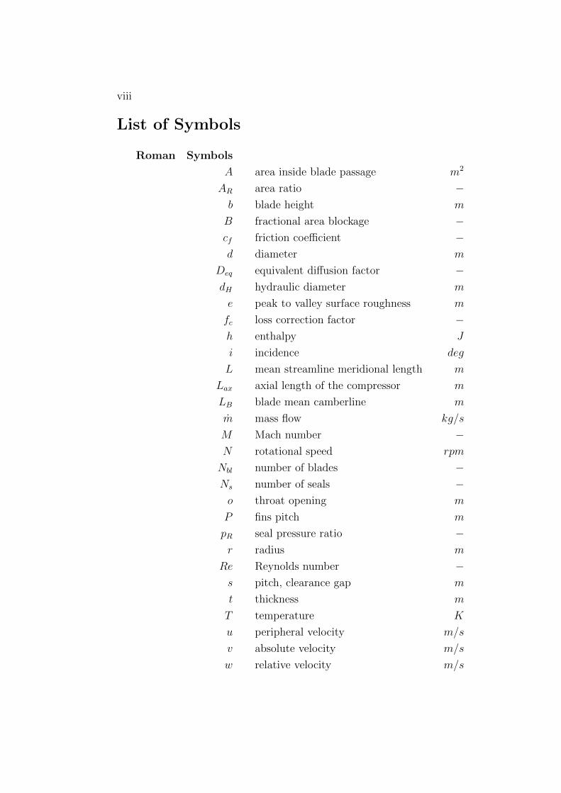
List of Symbols
Roman Symbols
A area inside blade passage m2
AR area ratio −b blade height m
B fractional area blockage −cf friction coefficient −d diameter m
Deq equivalent diffusion factor −dH hydraulic diameter m
e peak to valley surface roughness m
fc loss correction factor −h enthalpy J
i incidence deg
L mean streamline meridional length m
Lax axial length of the compressor m
LB blade mean camberline m
m mass flow kg/s
M Mach number −N rotational speed rpm
Nbl number of blades −Ns number of seals −o throat opening m
P fins pitch m
pR seal pressure ratio −r radius m
Re Reynolds number −s pitch, clearance gap m
t thickness m
T temperature K
u peripheral velocity m/s
v absolute velocity m/s
w relative velocity m/s
ix
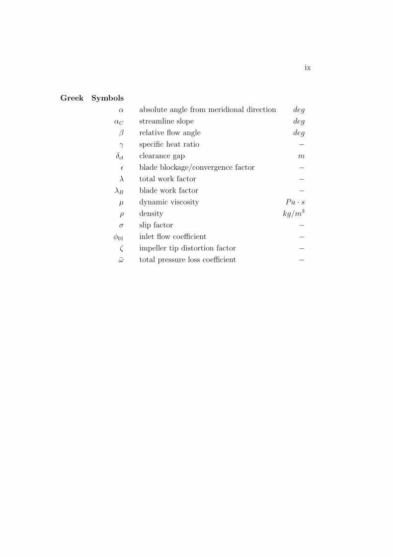
Greek Symbols
α absolute angle from meridional direction deg
αC streamline slope deg
β relative flow angle deg
γ specific heat ratio −δcl clearance gap m
ε blade blockage/convergence factor −λ total work factor −λB blade work factor −µ dynamic viscosity Pa · sρ density kg/m3
σ slip factor −φ01 inlet flow coefficient −ζ impeller tip distortion factor −ω total pressure loss coefficient −
x
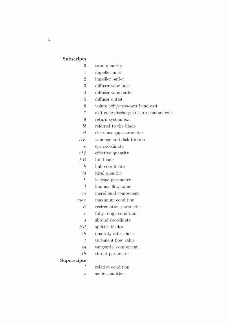
Subscripts
0 total quantity
1 impeller inlet
2 impeller outlet
3 diffuser vane inlet
4 diffuser vane outlet
5 diffuser outlet
6 volute exit/cross-over bend exit
7 exit cone discharge/return channel exit
8 return system exit
bl referred to the blade
cl clearance gap parameter
DF windage and disk friction
e eye coordinate
eff effective quantity
FB full blade
h hub coordinate
id ideal quantity
L leakage parameter
l laminar flow value
m meridional component
max maximum condition
R recirculation parameter
r fully rough condition
s shroud coordinate
SP splitter blades
sh quantity after shock
t turbulent flow value
tg tangential component
th throat parameter
Superscipts′ relative condition
∗ sonic condition
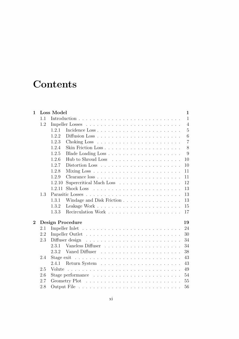
Contents
1 Loss Model 11.1 Introduction . . . . . . . . . . . . . . . . . . . . . . . . . . . . 11.2 Impeller Losses . . . . . . . . . . . . . . . . . . . . . . . . . . 4
1.2.1 Incidence Loss . . . . . . . . . . . . . . . . . . . . . . . 51.2.2 Diffusion Loss . . . . . . . . . . . . . . . . . . . . . . . 61.2.3 Choking Loss . . . . . . . . . . . . . . . . . . . . . . . 71.2.4 Skin Friction Loss . . . . . . . . . . . . . . . . . . . . . 81.2.5 Blade Loading Loss . . . . . . . . . . . . . . . . . . . . 91.2.6 Hub to Shroud Loss . . . . . . . . . . . . . . . . . . . 101.2.7 Distortion Loss . . . . . . . . . . . . . . . . . . . . . . 101.2.8 Mixing Loss . . . . . . . . . . . . . . . . . . . . . . . . 111.2.9 Clearance loss . . . . . . . . . . . . . . . . . . . . . . . 111.2.10 Supercritical Mach Loss . . . . . . . . . . . . . . . . . 121.2.11 Shock Loss . . . . . . . . . . . . . . . . . . . . . . . . 13
1.3 Parasitic Losses . . . . . . . . . . . . . . . . . . . . . . . . . . 131.3.1 Windage and Disk Friction . . . . . . . . . . . . . . . . 131.3.2 Leakage Work . . . . . . . . . . . . . . . . . . . . . . . 151.3.3 Recirculation Work . . . . . . . . . . . . . . . . . . . . 17
2 Design Procedure 192.1 Impeller Inlet . . . . . . . . . . . . . . . . . . . . . . . . . . . 242.2 Impeller Outlet . . . . . . . . . . . . . . . . . . . . . . . . . . 302.3 Diffuser design . . . . . . . . . . . . . . . . . . . . . . . . . . 34
2.3.1 Vaneless Diffuser . . . . . . . . . . . . . . . . . . . . . 342.3.2 Vaned Diffuser . . . . . . . . . . . . . . . . . . . . . . 38
2.4 Stage exit . . . . . . . . . . . . . . . . . . . . . . . . . . . . . 432.4.1 Return System . . . . . . . . . . . . . . . . . . . . . . 43
2.5 Volute . . . . . . . . . . . . . . . . . . . . . . . . . . . . . . . 492.6 Stage performance . . . . . . . . . . . . . . . . . . . . . . . . 542.7 Geometry Plot . . . . . . . . . . . . . . . . . . . . . . . . . . 552.8 Output File . . . . . . . . . . . . . . . . . . . . . . . . . . . . 56
xi
xii CONTENTS
3 Off Design Performance Maps 573.1 Pressure Ratio Map . . . . . . . . . . . . . . . . . . . . . . . . 583.2 Efficiency Map . . . . . . . . . . . . . . . . . . . . . . . . . . 613.3 Procedure in CCD . . . . . . . . . . . . . . . . . . . . . . . . 63
4 Validation 674.1 3 stages IGCC . . . . . . . . . . . . . . . . . . . . . . . . . . . 68
4.1.1 Off-Design IGCC . . . . . . . . . . . . . . . . . . . . . 724.1.2 Match of first stage . . . . . . . . . . . . . . . . . . . . 75
4.2 5 Stages Process Compressor . . . . . . . . . . . . . . . . . . . 784.2.1 Off-design 5 stages . . . . . . . . . . . . . . . . . . . . 804.2.2 6 Stages Hydrogen compressor . . . . . . . . . . . . . . 844.2.3 Flow coefficient match . . . . . . . . . . . . . . . . . . 86
4.3 High Efficiency Centrifugal Compressor (HECC) . . . . . . . . 884.3.1 Off-design . . . . . . . . . . . . . . . . . . . . . . . . . 92
4.4 Summary of Validation Tests . . . . . . . . . . . . . . . . . . 96
5 Conclusions 975.1 Future Works . . . . . . . . . . . . . . . . . . . . . . . . . . . 98
6 References 99
List of Figures
1.1 CCD Scheme . . . . . . . . . . . . . . . . . . . . . . . . . . . 2
1.2 Files for CCD . . . . . . . . . . . . . . . . . . . . . . . . . . . 3
1.3 h-s diagram . . . . . . . . . . . . . . . . . . . . . . . . . . . . 4
1.4 Sketch of blade throat opening . . . . . . . . . . . . . . . . . . 7
1.5 Blade surface velocity profile . . . . . . . . . . . . . . . . . . . 12
1.6 Typical geometry of a straight-through labyrinth seal . . . . . 16
2.1 Example of input file for CCD . . . . . . . . . . . . . . . . . . 20
2.2 Settings file . . . . . . . . . . . . . . . . . . . . . . . . . . . . 21
2.3 Initial design procedure in case of first stage of a shaft . . . . 23
2.4 Initial design procedure in case of following stages . . . . . . . 23
2.5 Section of a generic impeller of a centrifugal compressor . . . . 25
2.6 Zoom of the region between eye of the compressor and bladeinlet . . . . . . . . . . . . . . . . . . . . . . . . . . . . . . . . 25
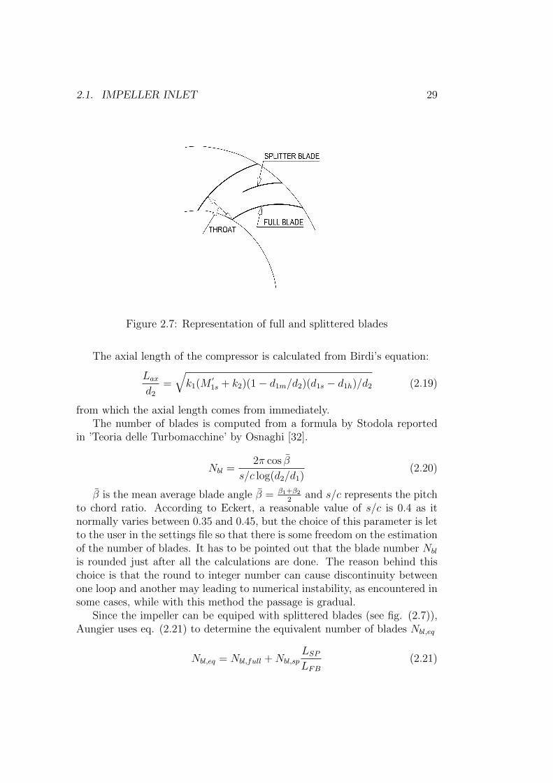
2.7 Representation of full and splittered blades . . . . . . . . . . . 29
2.8 Blade exit angle according to flow coefficient . . . . . . . . . . 30
2.9 Exit velocity triangle . . . . . . . . . . . . . . . . . . . . . . . 32
2.10 Thermodynamic transformations across the impeller . . . . . . 33
2.11 Sketch of impeller followed by a parallel wall diffuser . . . . . 36
2.12 Sketch of impeller followed by a vaned diffuser . . . . . . . . . 39
2.13 General shape of a return system . . . . . . . . . . . . . . . . 44
2.14 Geometry of a circular external volute . . . . . . . . . . . . . 50
2.15 Geometry of a circular semi-external volute . . . . . . . . . . . 50
2.16 Geometry of a rectangular internal volute . . . . . . . . . . . . 51
2.17 General Shape of the volute . . . . . . . . . . . . . . . . . . . 51
2.18 Exit cone . . . . . . . . . . . . . . . . . . . . . . . . . . . . . 54
2.19 Example of the layout of a five stage compressor as generatedby CCD . . . . . . . . . . . . . . . . . . . . . . . . . . . . . . 55
2.20 Example of output file gathering the most important stageparameters . . . . . . . . . . . . . . . . . . . . . . . . . . . . . 56
xiii
xiv LIST OF FIGURES
3.1 Flow coefficient correction for vaned turbocharger . . . . . . . 593.2 Off-design efficiency correction . . . . . . . . . . . . . . . . . . 593.3 Flow coefficient correction at low design Mach number for
vaneless stages . . . . . . . . . . . . . . . . . . . . . . . . . . . 603.4 Efficiency correction with tip-speed Mach numbers . . . . . . 613.5 Input file for the performance maps . . . . . . . . . . . . . . . 633.6 Variation of the peak flow coefficient with respect to that at
choke . . . . . . . . . . . . . . . . . . . . . . . . . . . . . . . . 643.7 Variation of the surge flow coefficient with respect to that at
choke . . . . . . . . . . . . . . . . . . . . . . . . . . . . . . . . 653.8 Example of efficiency performance map . . . . . . . . . . . . . 653.9 Example of pressure ratio performance map . . . . . . . . . . 66
4.1 3 stage geometry plot . . . . . . . . . . . . . . . . . . . . . . . 694.2 Comparison off CCDV03 maps with tests . . . . . . . . . . . . 734.3 Comparison of CCD V03 maps with CCD V01 . . . . . . . . . 744.4 3 stages IGCC geometry with matching input . . . . . . . . . 754.5 5 stages efficiency map with test data . . . . . . . . . . . . . . 814.6 5 stages pressure ratio map with test data . . . . . . . . . . . 814.7 5 stages PR map with speed correction . . . . . . . . . . . . . 824.8 5 stages efficiency map of 100% speedline . . . . . . . . . . . . 824.9 5 stages pressure ratio map of 100% speedline . . . . . . . . . 834.10 6 stages compressor geometry . . . . . . . . . . . . . . . . . . 844.11 Efficiency and PR maps comparison for the 6 stages case . . . 854.12 Efficiency and PR maps comparison for the 6 stages case with
φ01 match . . . . . . . . . . . . . . . . . . . . . . . . . . . . . 864.13 High Efficiency Centrifugal Compressor as modeled by NASA 884.14 High Efficiency Centrifugal Compressor as sketched by CCD . 894.15 HECC efficiency map of CCD V03 compared with test data,
CFD and CCD V01 . . . . . . . . . . . . . . . . . . . . . . . . 934.16 HECC pressure ratio map of CCD V03 compared with test data 934.17 Efficiency map comparison between CCD V03 and CFD re-
sults performed at VKI . . . . . . . . . . . . . . . . . . . . . . 944.18 Pressure ratio map comparison between CCD V03 and CFD
results performed at VKI . . . . . . . . . . . . . . . . . . . . . 95
List of Tables
4.1 IGCC comparison results . . . . . . . . . . . . . . . . . . . . . 704.2 IGCC results comparison with CCD V01 . . . . . . . . . . . . 714.3 IGCC off design constants . . . . . . . . . . . . . . . . . . . . 724.4 Value of off-design constants for low and high Mach numbers . 724.5 IGCC comparison between the output of CCD V03 and the
test data after matching . . . . . . . . . . . . . . . . . . . . . 764.6 IGCC comparison between the output of CCD V03 and CCD
V01 with the new geometry for first stage . . . . . . . . . . . 774.7 Comparison between CCD V03 and 5-stage compressor test
data . . . . . . . . . . . . . . . . . . . . . . . . . . . . . . . . 784.8 Comparison between CCD V03 and V01 for the 5-stage com-
pressor test case with the same input . . . . . . . . . . . . . . 794.9 5 stages off design paramters for blending function . . . . . . . 804.10 5 stages off design parameters . . . . . . . . . . . . . . . . . . 804.11 Data of 6 stage hydrogen compressor . . . . . . . . . . . . . . 844.12 Six stages compressor comparison between CCD V03 and V01
with φ01 = 0.027 . . . . . . . . . . . . . . . . . . . . . . . . . 854.13 Six stages efficiency comparison of CCD V03 and V01 with an
inlet flow coefficient for V03 of φ01 = 0.0181 . . . . . . . . . . 864.14 Suction parameters for HECC . . . . . . . . . . . . . . . . . . 884.15 HECC comparison between CCD V03 results and HECC data 904.16 HECC: Comparison between the results of CCD V03 and CCD
V01 . . . . . . . . . . . . . . . . . . . . . . . . . . . . . . . . 914.17 HECC paramters for blending function . . . . . . . . . . . . . 924.18 HECC: low and high limit for off-design parameters . . . . . . 92
xv

Chapter 1
Loss Model
1.1 Introduction
Even if nowadays the use of accurate CFD (Computational Fluid Dynamics)simulations for turbomachinery is massive, it is not true that it has sweptaway less sophisticated instruments from the repertoire of an engineer. Infact, during the first steps of the design phase, the designer usually relieson cheap and quick tools to obtain a reasonable preliminary sizing of themachine on which conduct, only later, more detailed analyses. These are theadvantages that a program like CCD can guarantee and that rise the interestin its further improvement.
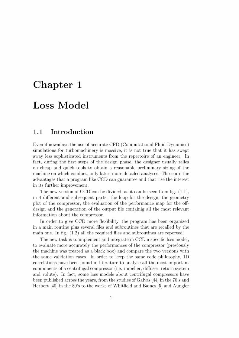
The new version of CCD can be divided, as it can be seen from fig. (1.1),in 4 different and subsequent parts: the loop for the design, the geometryplot of the compressor, the evaluation of the performance map for the off-design and the generation of the output file containig all the most relevantinformation about the compressor.
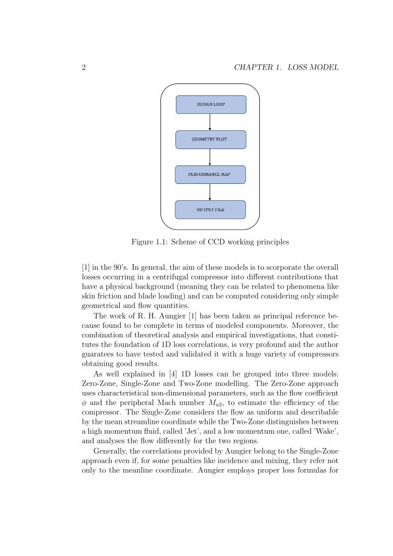
In order to give CCD more flexibility, the program has been organizedin a main routine plus several files and subroutines that are recalled by themain one. In fig. (1.2) all the required files and subroutines are reported.
The new task is to implement and integrate in CCD a specific loss model,to evaluate more accurately the performances of the compressor (previouslythe machine was treated as a black box) and compare the two versions withthe same validation cases. In order to keep the same code philosophy, 1Dcorrelations have been found in literature to analyse all the most importantcomponents of a centrifugal compressor (i.e. impeller, diffuser, return systemand volute). In fact, some loss models about centrifugal compressors havebeen published across the years, from the studies of Galvas [44] in the 70’s andHerbert [40] in the 80’s to the works of Whitfield and Baines [5] and Aungier
1
2 CHAPTER 1. LOSS MODEL
Figure 1.1: Scheme of CCD working principles
[1] in the 90’s. In general, the aim of these models is to scorporate the overalllosses occurring in a centrifugal compressor into different contributions thathave a physical background (meaning they can be related to phenomena likeskin friction and blade loading) and can be computed considering only simplegeometrical and flow quantities.
The work of R. H. Aungier [1] has been taken as principal reference be-cause found to be complete in terms of modeled components. Moreover, thecombination of theoretical analysis and empirical investigations, that consti-tutes the foundation of 1D loss correlations, is very profound and the authorguaratees to have tested and validated it with a huge variety of compressorsobtaining good results.
As well explained in [4] 1D losses can be grouped into three models:Zero-Zone, Single-Zone and Two-Zone modelling. The Zero-Zone approachuses characteristical non-dimensional parameters, such as the flow coefficientφ and the peripheral Mach number Mu2, to estimate the efficiency of thecompressor. The Single-Zone considers the flow as uniform and describableby the mean streamline coordinate while the Two-Zone distinguishes betweena high momentum fluid, called ’Jet’, and a low momentum one, called ’Wake’,and analyses the flow differently for the two regions.
Generally, the correlations provided by Aungier belong to the Single-Zoneapproach even if, for some penalties like incidence and mixing, they refer notonly to the meanline coordinate. Aungier employs proper loss formulas for
1.1. INTRODUCTION 3
Figure 1.2: Overview of the files needed by the CCD
the vaned components like the impeller, the vaned diffuser and return vanechannel while, as it will be later explained, exploits 1D governing equations,such as momentum, energy and gas state, for the vaneless spaces of thecompressor.
4 CHAPTER 1. LOSS MODEL
1.2 Impeller Losses
It has to be pointed out that, when dealing with the only rotating compo-nent of the compressor as the impeller is, the velocity to be considered (andtherefore all the depending quantities) is the relative and not the absoluteone as for all the others, following the kinematic relationship ~v = ~w + ~u.
The impeller model of Aungier is based on the total pressure loss coeffi-cients ω to find the real exit relative total pressure p
′02 using the relative inlet
total pressure p′01 and a correction factor fc:
p′
02 = p′
02,id − fc(p′
01 − p1)∑i=1
ωi (1.1)
As stated by the author himself, a total pressure loss coefficient is moreaccurate than an enthalpy based one because it is not dependent upon thepressure ratio involved.
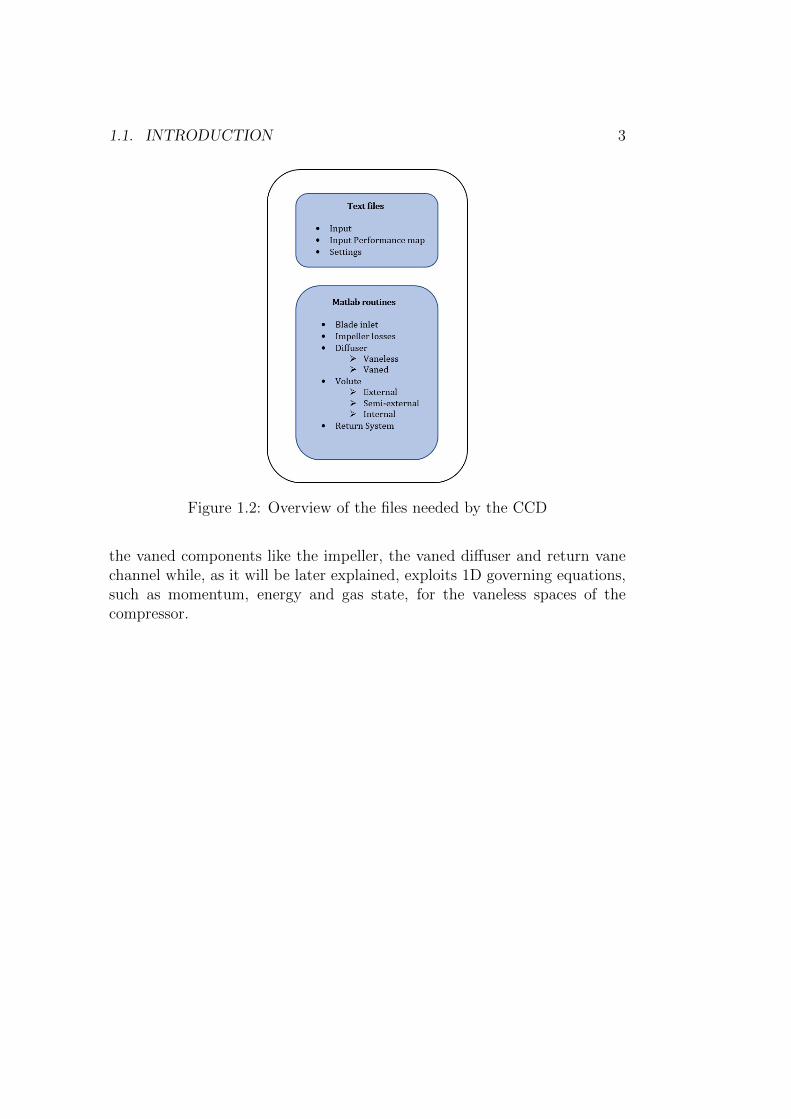
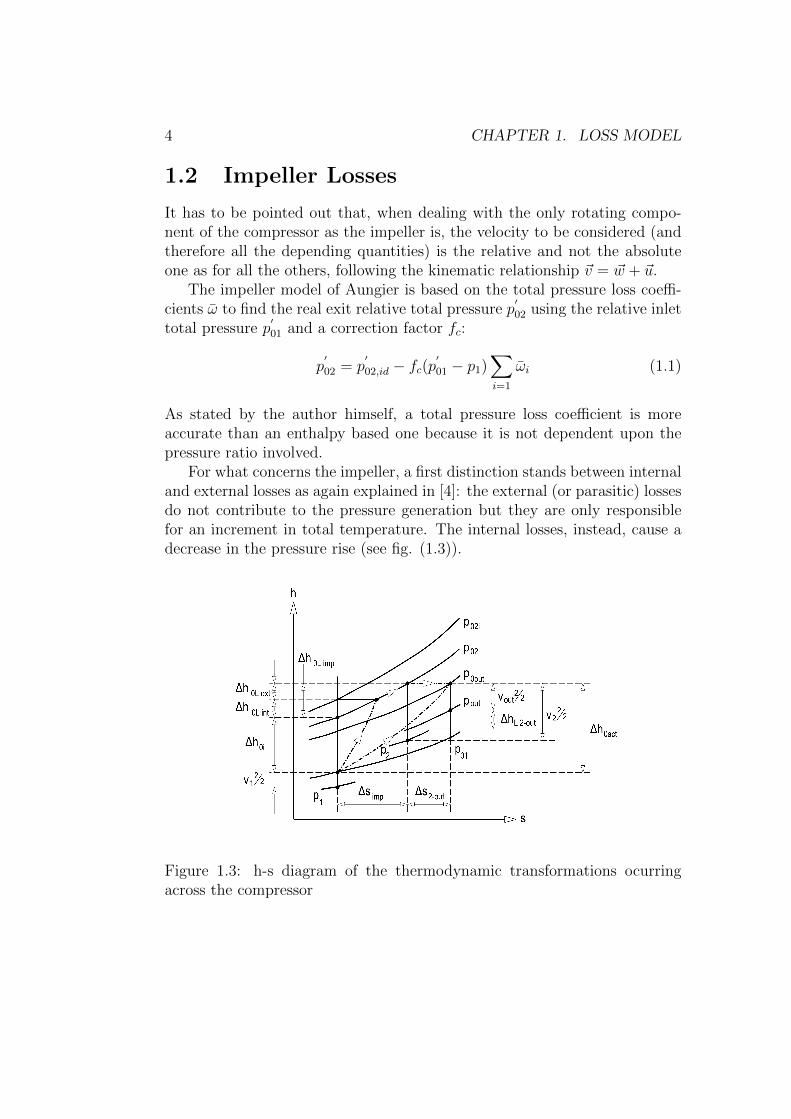
For what concerns the impeller, a first distinction stands between internaland external losses as again explained in [4]: the external (or parasitic) lossesdo not contribute to the pressure generation but they are only responsiblefor an increment in total temperature. The internal losses, instead, cause adecrease in the pressure rise (see fig. (1.3)).
Figure 1.3: h-s diagram of the thermodynamic transformations ocurringacross the compressor
1.2. IMPELLER LOSSES 5
The following internal losses are considered for the impeller as prescribedby Aungier:
• Incidence
• Clearance
• Skin friction
• Blade loading
• Hub to shroud
• Tip distortion
• Wake mixing
• Supercritical Mach number
• Diffusion
• Choking
• Shock
1.2.1 Incidence Loss
The correlation for the incidence loss is accounting for the flow adjustmentinto the blade passage as expressed by eq. (1.2). According to the conventionadopted, the angles are taken from the meridional direction, the opposite ofwhat done by Aungier, therefore the formulas have been changed to correctthis difference.
ωinc = 0.8[1− vm1/(w1 cos β1bl)]2 + [Nbl,fulltbl/(2πr1 cos β1bl)]
2 (1.2)
Eq. (1.2) is applied at hub, mid and shroud inlet stream surfaces and thetotal pressure incidence loss is computed as a weighted average, where themid values are weighted 10 times as heavy as the hub and shroud ones. Themeridional velocity at blade inlet is assumed to be uniform while the relativeangle changes along blade span according to the peripheral velocity. The firstterm is null in case of design point condition since w1 cos β1bl is exactly vm1 asβ1bl is chosen to be equal to design β1 (so optimal incidence i1,opt is equal tozero). On the other hand, this part will become relevant when dealing with
6 CHAPTER 1. LOSS MODEL
off-design conditions due to the onset of a perpendicular component hittingdirectly the blade. The second contribution to the incidence loss, instead,consideres the effect of abrupt flow area contraction at the blade leading edgedue to the latters thickness. Nbl,full distinguishes the number of full bladessince, as will be explained in chapter 2, also splittered blades can be present.
1.2.2 Diffusion Loss
The throat area is defined as the smallest section in a blade passage. Todischarge the same mass flow, the throat velocity wth has to be higher thanthe inlet meridional velocity w1m = w1 cos β1 as we can see comparing thetwo terms in eq. (1.7):
m = ρ1A1w1 cos β1 = ρthAthwth (1.3)
with the density term that will depend on the velocity itself. However, wth isusually lower than the inlet velocity w1 and so a deceleration, hence a diffu-sion of the flow, will occur. Since a dissipation is intrinsic in this process wemust account for a diffusion loss which is weighted according to the velocityratio wth/w1. The estimation of the throat area is one of the most difficultchallenges in 1D preliminary design, also because a detailed geometry profileis inherently missing in a 1D approach. Therefore, a simplified procedureproposed by Whitfield and Baines will be employed. At first, no differencebetween inlet and throat sections is considered in terms of radial extent, sothat the throat height equals the inlet blade height b1. Because of this hy-pothesis, to satisfy rothalpy conservation (see eq. (1.4)) the relative total
temperature(T′1 = T1 +
w21
2cp
)is constant between the two sections.
h1 + w21/2− u2
1/2 = hth + w2th/2− u2
th/2 (1.4)
Moreover, the flow is considered to be isentropic between inlet and throatsections and so also the relative total pressure and density are constant. Aslightly different approach is adopted in case of supersonic entrance flow. Inthat situation, a normal shock is considered to occur when M
′1 > 1, as pro-
posed both by Aungier and Whitlfield and Baines. The isentropic relationsare then applied starting from the conditions just after the discontinuity,where the relative total temperature is equal to the upstream one but thetotal pressure is lower and the Mach number turned to be subsonic. Subse-quently, the throat opening ’o’ is computed as it would be a side of a rectan-gular triangle with hypotenuse the pitch ’s’, found as s = πd1/Nbl,full − tbl,1.
o = s cos β1,bl (1.5)
1.2. IMPELLER LOSSES 7
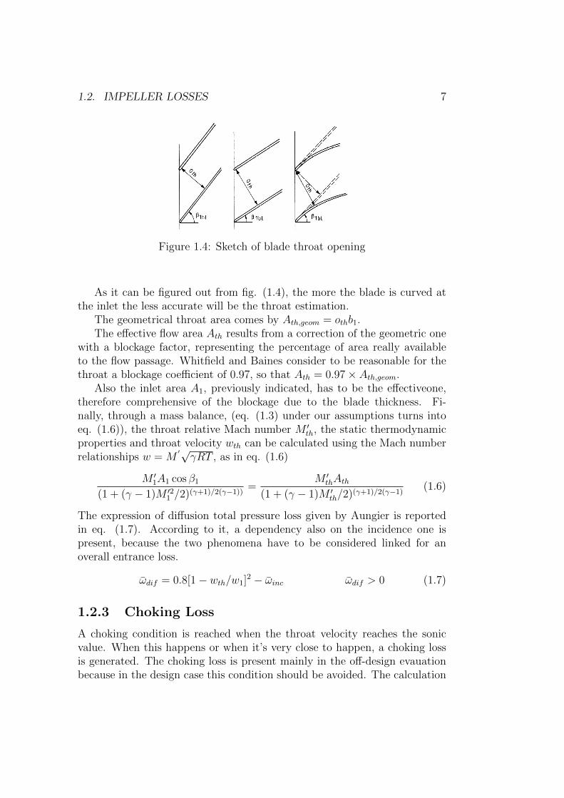
Figure 1.4: Sketch of blade throat opening
As it can be figured out from fig. (1.4), the more the blade is curved atthe inlet the less accurate will be the throat estimation.
The geometrical throat area comes by Ath,geom = othb1.The effective flow area Ath results from a correction of the geometric one
with a blockage factor, representing the percentage of area really availableto the flow passage. Whitfield and Baines consider to be reasonable for thethroat a blockage coefficient of 0.97, so that Ath = 0.97× Ath,geom.
Also the inlet area A1, previously indicated, has to be the effectiveone,therefore comprehensive of the blockage due to the blade thickness. Fi-nally, through a mass balance, (eq. (1.3) under our assumptions turns intoeq. (1.6)), the throat relative Mach number M ′
th, the static thermodynamicproperties and throat velocity wth can be calculated using the Mach numberrelationships w = M
′√γRT , as in eq. (1.6)
M ′1A1 cos β1
(1 + (γ − 1)M ′21 /2)(γ+1)/2(γ−1))
=M ′
thAth(1 + (γ − 1)M ′
th/2)(γ+1)/2(γ−1)(1.6)
The expression of diffusion total pressure loss given by Aungier is reportedin eq. (1.7). According to it, a dependency also on the incidence one ispresent, because the two phenomena have to be considered linked for anoverall entrance loss.
ωdif = 0.8[1− wth/w1]2 − ωinc ωdif > 0 (1.7)
1.2.3 Choking Loss
A choking condition is reached when the throat velocity reaches the sonicvalue. When this happens or when it’s very close to happen, a choking lossis generated. The choking loss is present mainly in the off-design evauationbecause in the design case this condition should be avoided. The calculation
8 CHAPTER 1. LOSS MODEL
of the sonic area A∗, the area leading to sonic velocity with fixed mass flowand static temperature, is again derived from eq. (1.6) with M
′
th = 1 andthen compared to the effective throat area. Aungier employs the parameterXch = 11− 10Ath/A
∗ to find the choking loss (when Xch > 0):
ωch =1
2
(0.05Xch +X7
ch
)(1.8)
1.2.4 Skin Friction Loss
One of the most common source of losses is skin friction between the fluidand the metal surfaces that Aungier recalls in eq. (1.9).
ωsf = 4cf
(w
w1
)2
LB/dH (1.9)
w2 =w2
1+w22
2represents the root mean square velocity.
As the majority of the experiments regarding friction were conducted inpipe flows, it is common practice to reconduct usual turbomachine passagesto equivalent pipe quantities (hence hydraulic quantities) to be consistentwith the data taken from them. dH is the the hydraulic diameter whichAungier refers to as the average of the tip and throat one based on thecommon expression:
hydraulic diameter = 4cross sectional area
wetted peremeter(1.10)
The computation of the hydraulic diameters at throat follows:
dH1 =4Ath
2(b1 + s cos β1)Nbl,full
(1.11)
and at tip becomes:
dH2 =4πd2b2/Nbl
2πd2/Nbl + 2b2
(1.12)
The friction coefficient cf is evaluated by Aungier according to the on-going flow regime. As usual, it will depend mainly on two parameters: theReynolds number Red = ρ1u2dH/µ1 and the peak to valley surface roughnesse (a value of e = 5 has been assumed as reference µm but the possibility tomodify it has been provided in the settings file. The tip peripheral velocity u2
has been employed for the calculation of the Reynolds number following theguidelines of the work of R. A. Van Den Braembussche [11]. If Red < 2000
1.2. IMPELLER LOSSES 9
the flow regime is laminar and, since roughness plays no role, the frictioncoefficient can be expressed by cf = cfl = 16/Red. In the transition zone(i.e. 2000 < Red < 4000 instead, cf is assessed by another equation havingthe laminar (cfl) and turbulent (cft) friction coefficients as extreme values:
cf = cfl + (cft − cfl)(Red/2000− 1) (1.13)
When Red > 4000 the flow is turbulent but a distinction has to be pointedout between smooth and rough surfaces conditions. In reality, the surfacecannot be perfectly smooth but it can thus be considered when the laminarsub-layer fully contains the roughness peaks. The turbulent smooth frictioncoefficient cfts is modeled by
1√4cfts
= −2log10
[2.51
Red√
4cfts
](1.14)
while the turbulent rough friction coefficient cftr value is taken from:
1√4cftr
= −2log10
[e
3.71d
](1.15)
To establish which effect roughness is playing a roughness-based Reynoldsnumber Ree is evaluated according to Ree = (Red−2000)e/d. The turbulentskin friction coefficient then becomes:
cf = cfts Ree < 60 (1.16)
cf = cfts + (cftr − cfts)(60/Ree) Ree ≥ 60 (1.17)
1.2.5 Blade Loading Loss
Another main source of loss in centrifugal compressors is represented by theblade loading, which is related to blade-to-blade pressure gradients. It isstrongly dependent on the solidity, i.e. the chord to pitch ratio. In fact,given a certain force to be imparted to the fluid, correlated to the passagemass flow and tangential velocity deflection, blade loading will increase if thenumber or length of the blade decrease and viceversa. An excessive loadingcan lead to boundary layer growth and flow detachment in the impeller,causing a great amount of losses. A parameter representing the loading isthe maximum velocity difference:
∆w =2πd2u2λBNbl,effLB
(1.18)
10 CHAPTER 1. LOSS MODEL
where λB is the blade work factor, Nbl,eff is the effective number of bladesand the blade mean camberline. The final pressure loss given by Aungierweights the maximum velocity difference with respect to the inlet relativeone as it can be seen from eq. (1.19)
ωbl = (∆w/w1)2/24 (1.19)
1.2.6 Hub to Shroud Loss
As blade loading loss is related to pressure gradients among the blades, thehub to shroud loss is related to the presence of pressure gradients alongthe blade span due to radial equilibrium issues. The hub to shroud lossschematized by Aungier considers the streamline curvature km = αC2−αC1
Lin
the meridional plane between inlet and exit of the blade, therefore referringto blade inlet and outlet velocities for the calculations in eq. (1.20)
ωhs = (kmbw/w1)2/6 (1.20)
αC1 and αC2 are the streamline slope angles with the axis. The inlet oneis calculated in the blade inlet routine according to the input provided while,since the outlet is always perfectly radial, it will be αC2 = 0. The meridionallength L is approximated by L ≈ d2/2− (dE/2 + r) + (r+ b1/2)(π/2− αC1),where r is the shroud radius of curvature of the blade at inlet.
A distinction on blade length has to be made here. Since the shapeof the blade is in general fully three-dimensional, different lengths can beconsidered. L is the meridional length which considers the extension of theblade in the meridional plane and LB is the blade mean camberline, evaluatedon the secondary plane accounting also for the curvature due to backwardorientation and inlet swirl of the blade.
1.2.7 Distortion Loss
Aungier assesses that the impeller tip meridional velocity profile distortioncan be expected to contribute to a loss modelable as an abrupt expansion.The tip distortion factor ζ is:
ζ =1
1−B2
(1.21)
Tip blockage B2 is a very important parameter representing the boundarylayer blockage at tip and it is comprehensive of lots of contributions (skinfriction, area ratio ecc.) as it can be seen by eq. (1.22).
B2 = ωsfp01 − p1
p02 − p2
√w1dHw2b2
+
[0.3 +
b22
L2B
]A2Rρ2b2
ρ1LB+δcl2b2
(1.22)

1.2. IMPELLER LOSSES 11
δcl is the clearance gap (fixed in the setting file, default 0.5 mm) applied onlyin case of open impellers and the area ratio AR is defined as:
AR = A2 cos β2,bl/A1 cos β1,bl (1.23)
The distortion loss weights the meridional velocity component on the relativeinlet velocity as expressed by eq. (1.24)
ωdis = [(ζ − 1)vm2/w1]2 (1.24)
1.2.8 Mixing Loss
It has been analysed that in compressors the low momentum fluid tends toconcentrate in a small region on tip suction side, called wake, while the otherpart, called jet, is the free stream and isentropic one. Once the blade ends,the two regions mix together causing a loss due to developing drag forces.Aungier first evaluates the magnitude of the wake velocity with the estima-tion of the velocity at which separation occurs. This is done considering theequivalent diffusion factor Deq = wmax
w2, with wmax = (w1 + w2 + ∆w)/2.
wsep = w2 Deq ≤ 2 (1.25)
wsep = w2Deq/2 Deq > 2 (1.26)
The mixing involves only the meridional component of the velocity and Vm,mixis found by
vm,mix = vm2A2/πd2b2 (1.27)
After the blade trailing edge, the available area rises as the blades thicknessdoes not cause blockage anymore hence the meridional mix velocity will beslightly lower than V2m. A2 is the area inside blade passage at impeller exitcomputed as A2 = πb2d2ε2 and ε2 = 1− Nbltb
πd2blade blockage at exit
vm,wake =√w2sep − w2
2,tg (1.28)
The wake mixing loss, similar to another abrupt expansion loss, is givenby eq. (1.29)
ωmix = [(vm,wake − vm,mix)/w1]2 (1.29)
1.2.9 Clearance loss
Clearance loss applies only to open impellers as in this case flow can leakfrom one blade passage to another due to blade-to-blade pressure difference.
12 CHAPTER 1. LOSS MODEL
The blade pressure difference ∆pcl and clearance gap leaking flow will yielda total pressure loss given by eq. (1.30)
ωcl =2mcl∆pclmρ1w2
1
(1.30)
∆pcl is found by the moment of momentum variation by:
∆pcl =m(d2v2,tg − d1v1,tg)
Nbl,eff dbL(1.31)
ucl is the flow velocity across the gap and mcl is the mass leaking in theclearance is
ucl = 0.816√
2∆pcl/ρ2 (1.32)
mcl = ρ2Nbl,effsLucl (1.33)
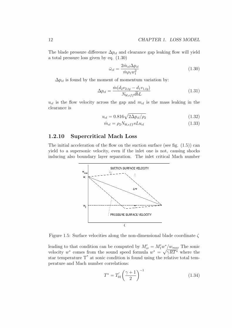
1.2.10 Supercritical Mach Loss
The initial acceleration of the flow on the suction surface (see fig. (1.5)) canyield to a supersonic velocity, even if the inlet one is not, causing shocksinducing also boundary layer separation. The inlet critical Mach number
Figure 1.5: Surface velocities along the non-dimensional blade coordinate ζ
leading to that condition can be computed by M ′cr = M ′
1w∗/wmax The sonic
velocity w∗ comes from the sound speed formula w∗ =√γRT ∗ where the
star temperature T* at sonic condition is found using the relative total tem-perature and Mach number correlations:
T ∗ = T′
01
(γ + 1
2
)−1
(1.34)
1.3. PARASITIC LOSSES 13
The supercritical Mach number loss set by Aungier is:
ωcr = 0.4[(M ′1 −M ′
cr)wmax/w1]2 (1.35)
1.2.11 Shock Loss
Whitfield and Baines report that no total pressure loss correlation for inletshock losses are available in literature, therefore a new procedure will beadopted. As suggested by the authors, the shock is considered to be normaland this hypothesis allows to compute the thermodynamic quantities afterthe discontinuity using a Mach number based equations available in liter-ature. The relative total pressure just after the normal shock p′SH can befound as:
p′SH = p′01
[(γ + 1)M ′2
1
(γ − 1)M ′21 + 2
]γ/(γ−1)[(γ + 1)
2γM ′21 − (γ − 1)
]1/(γ−1)
(1.36)
From ∆p′SH , ∆p′01 will finally results.
ωSH = ∆p′0/(p′0 − p)1 (1.37)
1.3 Parasitic Losses
External losses comprehend three different cathegories:
• Windage and disk friction
• Leakage
• Recirculation
1.3.1 Windage and Disk Friction
The friction occurring between the rotating disk and the stationary housingis referred to as windage and disk friction. The work done by Daily and Nece(1960) is considered by Aungier as the best source available for this source ofloss. The dissertation is similar to the one for skin friction as a rotating diskin a housing for smooth and rough disks is treated. The torque coefficient isgiven by
CM =2τ
ρω2r5(1.38)
where τ is the torque due to friction and ω is the rotational speed. Thecoefficients will depend on the flow regime existing between the boundary
14 CHAPTER 1. LOSS MODEL
layer of the disk and the one of the housing, basing the criterion again on
the Reynolds number, here computed as Re =ρ2ωr22µ2
, four flow regimes are
considered and for each of them a specific torque coefficient (not consideringroughness yet) is set:
1. Laminar, merged boundary layers
CM1 =2π
(s/r)Re(1.39)
2. Laminar, separate boundary layers
CM2 =3.7(s/r)0.1
√Re
(1.40)
3. Turbulent, merged boundary layers
CM3 =0.08
(s/r)16Re
14
(1.41)
4. Turbulent, separate boundary layers
CM4 =0.102(s/r)0.1
Re0.2(1.42)
s is the gap between the disk and the housing and r the disk radius. A typicalvalue of 0.02 for the s over r ratio has been taken starting from indicationsgiven by Aungier. The smooth torque coefficient CMs can be evaluated bythe maximum value of the four torque coefficient and it will give an indicationon which is the existing flow regime. The disk can be considered as smoothtill a value of Res given by eq. (1.43)
Res√CMs = 1100(e/r)−0.4 (1.43)
The Reynolds number Rer at which roughness has no more effect is instead:
Rer = 1100r
e− 6 · 106 (1.44)
And the torque coefficient for fully rough disk is given by
1√CMr
= 3.8 log10
(r
e
)− 2.4
(s
r
)0.25
(1.45)
1.3. PARASITIC LOSSES 15
In the middle of the two regimes the torque coefficient is
CM = CMs + (CMr − CMs) log(Re/Res)/ log(Rer/Res) (1.46)
At this point, Aungier corrects these ideal disk torque coefficients to adaptthem to centrifugal compressor, setting a correction for the clearance gapleakage flows. Denoting the previous torque friction coefficient as CM0, thenew torque coefficient is:
CM = CM0(1−K)2/(1−K20) (1.47)
Where K is the clearance gap swirl parameter and K0 and Cq other clearanceparameters
K = K0 + Cq(1.75KF − 0.316)r2/s (1.48)
K0 = 0.46/(1 + 2s/d) (1.49)
Cq =m(ρ2r2u2/µ2)1/5
2πρ2r22u2
(1.50)
For seal leakage towards the tip the impeller tip swirl parameter KF can beevaluated by
KF = v2t/u2 (1.51)
otherwise KF = 0.The impeller disk friction torque coefficient is computed independently
for the disk and the cover and the results are adjusted by:
CMD = 0.75CM (for the disk) (1.52)
CMC = 0.75LCM
[1−
(d1e
d2
)5]/(r2 − r1) (for the cover) (1.53)
and then the windage and disk friction parasitic work is obtained from:
λDF = (CMD + CMC)ρ2u2r22/(2m) (1.54)
In case of uncovered impellers, the term CMC is not considered.
1.3.2 Leakage Work
Another parasitic loss is represented by the leakage across the eye and shaftseals and gaps. The computation of the leakage work requires the knowl-edge of the seal geometry, which is typically considered as a straight-throughlabyrinth seal. A schematization of the seal geometry is shown in fig. (1.6)
16 CHAPTER 1. LOSS MODEL
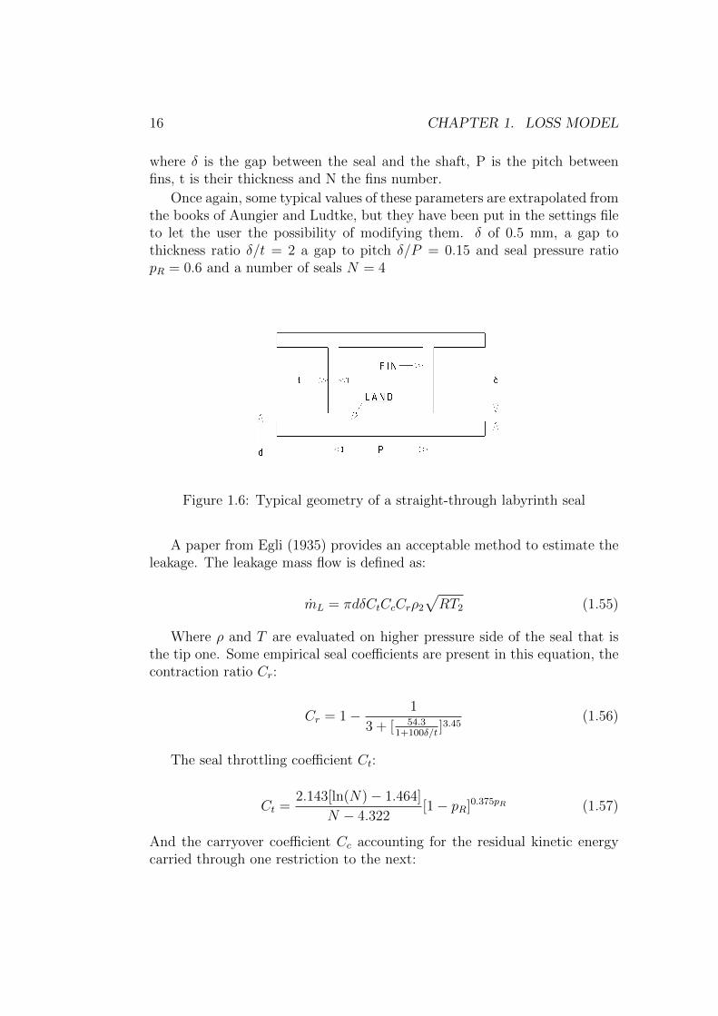
where δ is the gap between the seal and the shaft, P is the pitch betweenfins, t is their thickness and N the fins number.
Once again, some typical values of these parameters are extrapolated fromthe books of Aungier and Ludtke, but they have been put in the settings fileto let the user the possibility of modifying them. δ of 0.5 mm, a gap tothickness ratio δ/t = 2 a gap to pitch δ/P = 0.15 and seal pressure ratiopR = 0.6 and a number of seals N = 4
Figure 1.6: Typical geometry of a straight-through labyrinth seal
A paper from Egli (1935) provides an acceptable method to estimate theleakage. The leakage mass flow is defined as:
mL = πdδCtCcCrρ2
√RT2 (1.55)
Where ρ and T are evaluated on higher pressure side of the seal that isthe tip one. Some empirical seal coefficients are present in this equation, thecontraction ratio Cr:
Cr = 1− 1
3 + [ 54.31+100δ/t
]3.45(1.56)
The seal throttling coefficient Ct:
Ct =2.143[ln(N)− 1.464]
N − 4.322[1− pR]0.375pR (1.57)
And the carryover coefficient Cc accounting for the residual kinetic energycarried through one restriction to the next:
1.3. PARASITIC LOSSES 17
Cc = 1 +X1[δ/P −X2 ln(1 + δ/P )]
1−X2
(1.58)
X1 = 15.1− 0.05255 exp[0.507(12−N)] N ≤ 12 (1.59)
X1 = 13.15 + 0.1625N N > 12 (1.60)
X2 = 1.058 + 0.0218N N ≤ 12 (1.61)
X2 = 1.32 N > 12 (1.62)
(1.63)
The expression of the leakage work will depend on the impeller config-uration, if it is an open or a covered one. For covered impellers, Aungieraccounts for the fact that the leakage flow is worked on by the impeller asecond time:
λL =mLλBm
for covered impellers (1.64)
For open impellers, the assumption made is that half of the blade clear-ance leakage flow is reenergized by the impeller:
λL =mclucl2u2m
for open impellers (1.65)
1.3.3 Recirculation Work
Recirculation flow is related to incipient stall condition. In particular at lowmass flow rate, when the load becomes high, you can expect some backflowsgenerating wasted work. The Lieblein criterion for axial compressor with theequivalent diffusion factor Deq is used to predict stall when Deq > 2, even ifmost impellers can go beyond that. The recirculation work is:
λR =
(Deq
2− 1
)[w2t
v2m
+ 2 tan β2
]λR ≥ 0 (1.66)

Chapter 2
Design Procedure
The design of a compressor in CCD follows a sequential path so that theanalysis is carried out component after component and stage after stage,thanks to the fact that the outlet quantities of a component or stage are theinlet quantities of the next one, till the whole machine is completely solved.
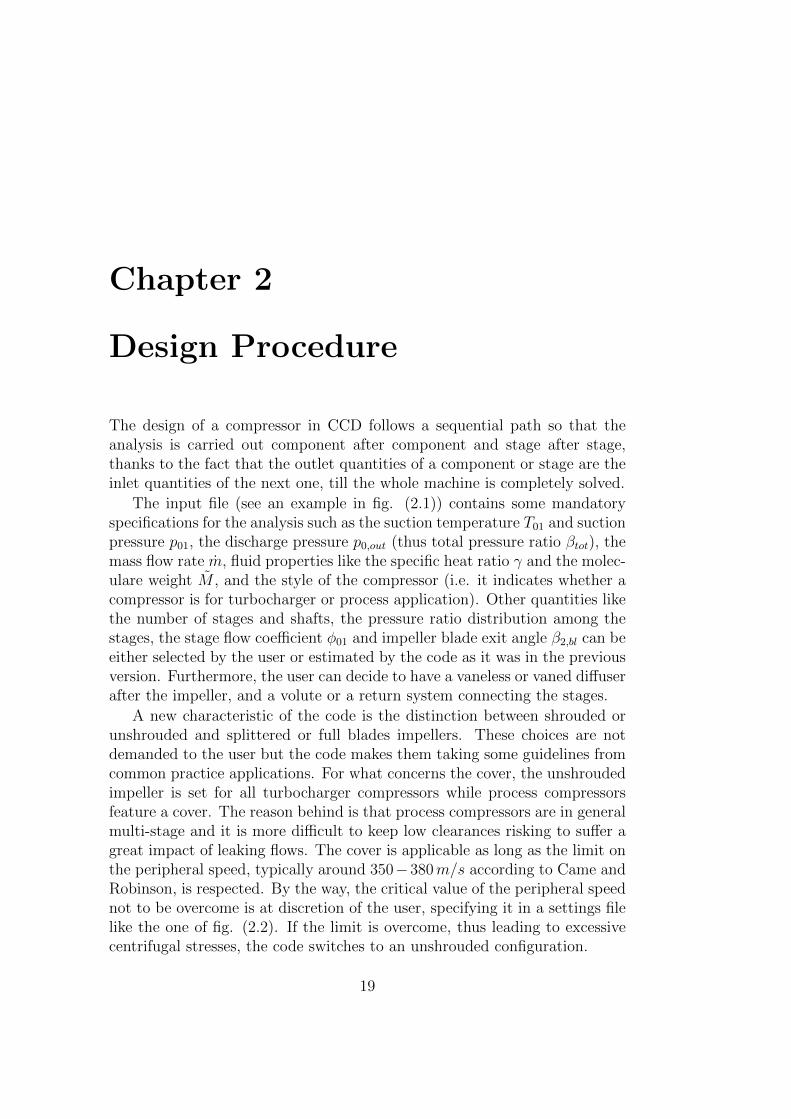
The input file (see an example in fig. (2.1)) contains some mandatoryspecifications for the analysis such as the suction temperature T01 and suctionpressure p01, the discharge pressure p0,out (thus total pressure ratio βtot), themass flow rate m, fluid properties like the specific heat ratio γ and the molec-ulare weight M , and the style of the compressor (i.e. it indicates whether acompressor is for turbocharger or process application). Other quantities likethe number of stages and shafts, the pressure ratio distribution among thestages, the stage flow coefficient φ01 and impeller blade exit angle β2,bl can beeither selected by the user or estimated by the code as it was in the previousversion. Furthermore, the user can decide to have a vaneless or vaned diffuserafter the impeller, and a volute or a return system connecting the stages.
A new characteristic of the code is the distinction between shrouded orunshrouded and splittered or full blades impellers. These choices are notdemanded to the user but the code makes them taking some guidelines fromcommon practice applications. For what concerns the cover, the unshroudedimpeller is set for all turbocharger compressors while process compressorsfeature a cover. The reason behind is that process compressors are in generalmulti-stage and it is more difficult to keep low clearances risking to suffer agreat impact of leaking flows. The cover is applicable as long as the limit onthe peripheral speed, typically around 350−380m/s according to Came andRobinson, is respected. By the way, the critical value of the peripheral speednot to be overcome is at discretion of the user, specifying it in a settings filelike the one of fig. (2.2). If the limit is overcome, thus leading to excessivecentrifugal stresses, the code switches to an unshrouded configuration.
19
20 CHAPTER 2. DESIGN PROCEDURE
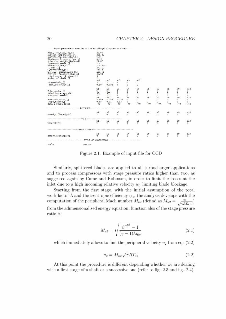
Figure 2.1: Example of input file for CCD
Similarly, splittered blades are applied to all turbocharger applicationsand to process compressors with stage pressure ratios higher than two, assuggested again by Came and Robinson, in order to limit the losses at theinlet due to a high incoming relative velocity w1 limiting blade blockage.
Starting from the first stage, with the initial assumption of the totalwork factor λ and the isentropic efficiency ηis, the analysis develops with thecomputation of the peripheral Mach number Mu2 (defind as Mu2 = u2√
γRT0,in)
from the adimensionalised energy equation, function also of the stage pressureratio β:
Mu2 =
√βγ−1γ − 1
(γ − 1)ληis(2.1)
which immediately allows to find the peripheral velocity u2 from eq. (2.2)
u2 = Mu2
√γRT01 (2.2)
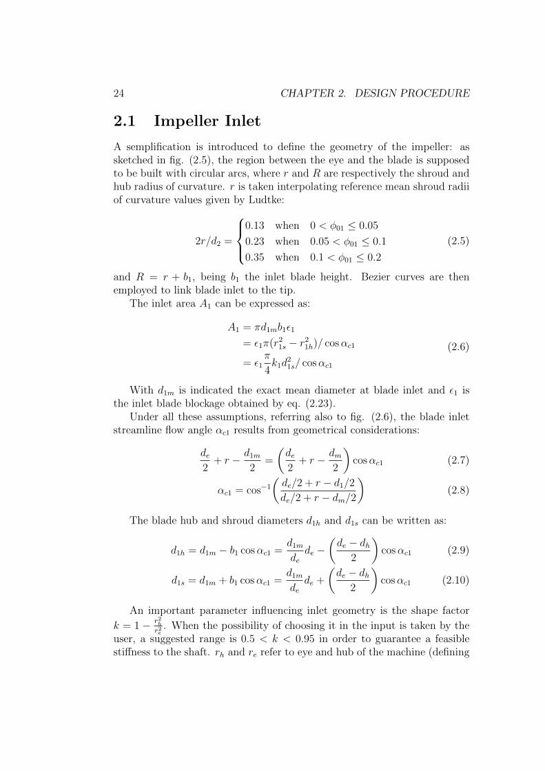
At this point the procedure is different depending whether we are dealingwith a first stage of a shaft or a successive one (refer to fig. 2.3 and fig. 2.4).
21
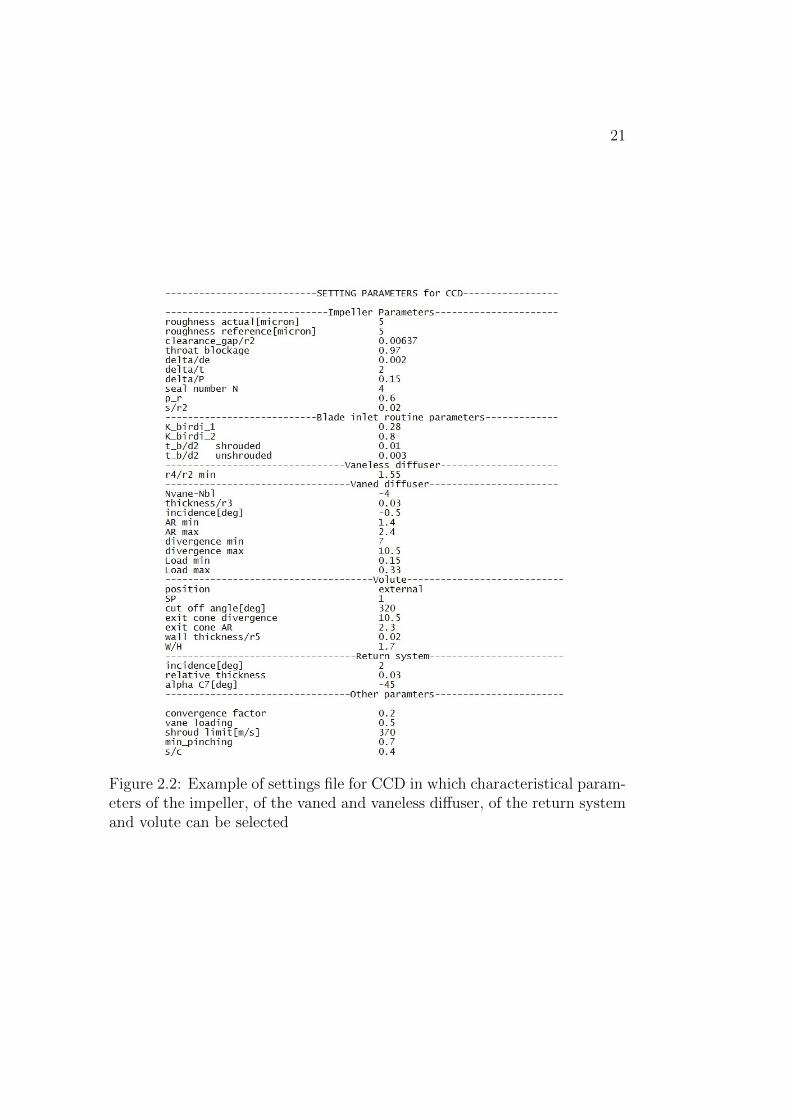
Figure 2.2: Example of settings file for CCD in which characteristical param-eters of the impeller, of the vaned and vaneless diffuser, of the return systemand volute can be selected
22 CHAPTER 2. DESIGN PROCEDURE
In the first case the inlet flow coefficient φ01
φ01 =V01
u2d22
(2.3)
(being V01 the total volumetric flow rate calculated as V01 = mρ01
) is fixedand the rotational speed N has to be found. In the other case, instead, Nis a constraint imposed by the first stage and φ01 is a result. The dischargetemperature T0,out is found rewriting the definiton of total work factor λ =cp(T0,out−T0,in)
u22, so that:
T0,out = T0,in + u22
λ
cp(2.4)
An additional guess, on λ, is needed since its value will be known at theend of the impeller procedure.
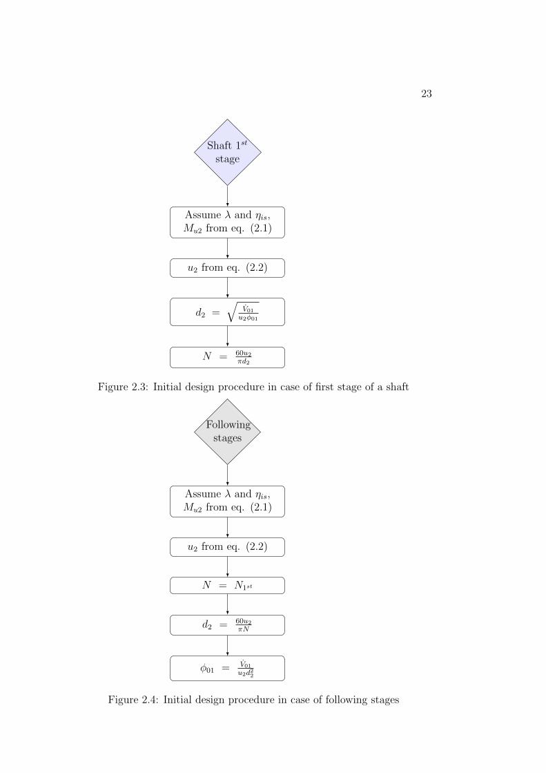
23
Shaft 1st
stage
Assume λ and ηis,Mu2 from eq. (2.1)
u2 from eq. (2.2)
d2 =√
V01u2φ01
N = 60u2πd2
Figure 2.3: Initial design procedure in case of first stage of a shaft
Followingstages
Assume λ and ηis,Mu2 from eq. (2.1)
u2 from eq. (2.2)
N = N1st
d2 = 60u2πN
φ01 = V01u2d22
Figure 2.4: Initial design procedure in case of following stages
24 CHAPTER 2. DESIGN PROCEDURE
2.1 Impeller Inlet
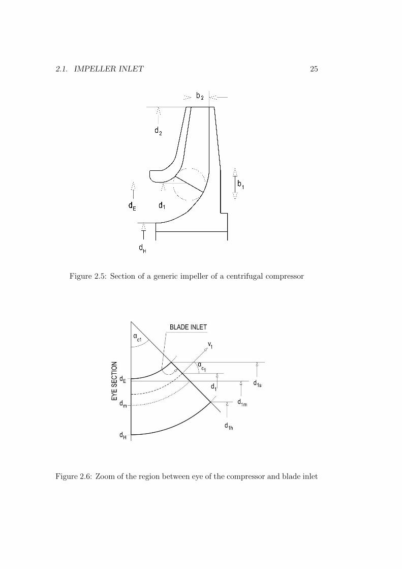
A semplification is introduced to define the geometry of the impeller: assketched in fig. (2.5), the region between the eye and the blade is supposedto be built with circular arcs, where r and R are respectively the shroud andhub radius of curvature. r is taken interpolating reference mean shroud radiiof curvature values given by Ludtke:
2r/d2 =
0.13 when 0 < φ01 ≤ 0.05
0.23 when 0.05 < φ01 ≤ 0.1
0.35 when 0.1 < φ01 ≤ 0.2
(2.5)
and R = r + b1, being b1 the inlet blade height. Bezier curves are thenemployed to link blade inlet to the tip.
The inlet area A1 can be expressed as:
A1 = πd1mb1ε1
= ε1π(r21s − r2
1h)/ cosαc1
= ε1π
4k1d
21s/ cosαc1
(2.6)
With d1m is indicated the exact mean diameter at blade inlet and ε1 isthe inlet blade blockage obtained by eq. (2.23).
Under all these assumptions, referring also to fig. (2.6), the blade inletstreamline flow angle αc1 results from geometrical considerations:
de2
+ r − d1m
2=
(de2
+ r − dm2
)cosαc1 (2.7)
αc1 = cos−1
(de/2 + r − d1/2
de/2 + r − dm/2
)(2.8)
The blade hub and shroud diameters d1h and d1s can be written as:
d1h = d1m − b1 cosαc1 =d1m
dede −
(de − dh
2
)cosαc1 (2.9)
d1s = d1m + b1 cosαc1 =d1m
dede +
(de − dh
2
)cosαc1 (2.10)
An important parameter influencing inlet geometry is the shape factor
k = 1− r2hr2e
. When the possibility of choosing it in the input is taken by theuser, a suggested range is 0.5 < k < 0.95 in order to guarantee a feasiblestiffness to the shaft. rh and re refer to eye and hub of the machine (defining
2.1. IMPELLER INLET 25
Figure 2.5: Section of a generic impeller of a centrifugal compressor
Figure 2.6: Zoom of the region between eye of the compressor and blade inlet
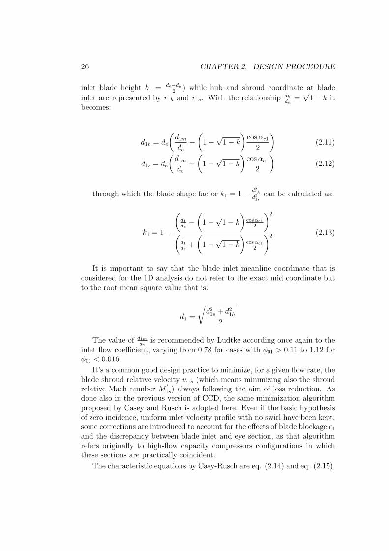
26 CHAPTER 2. DESIGN PROCEDURE
inlet blade height b1 = de−dh2
) while hub and shroud coordinate at blade
inlet are represented by r1h and r1s. With the relationship dhde
=√
1− k itbecomes:
d1h = de
(d1m
de−(
1−√
1− k)
cosαc12
)(2.11)
d1s = de
(d1m
de+
(1−√
1− k)
cosαc12
)(2.12)
through which the blade shape factor k1 = 1− d21hd21s
can be calculated as:
k1 = 1−
(d1de−(
1−√
1− k)
cosαc12
)2
(d1de
+
(1−√
1− k)
cosαc12
)2 (2.13)
It is important to say that the blade inlet meanline coordinate that isconsidered for the 1D analysis do not refer to the exact mid coordinate butto the root mean square value that is:
d1 =
√d2
1s + d21h
2
The value of d1mde
is recommended by Ludtke according once again to theinlet flow coefficient, varying from 0.78 for cases with φ01 > 0.11 to 1.12 forφ01 < 0.016.
It’s a common good design practice to minimize, for a given flow rate, theblade shroud relative velocity w1s (which means minimizing also the shroudrelative Mach number M
′1s) always following the aim of loss reduction. As
done also in the previous version of CCD, the same minimization algorithmproposed by Casey and Rusch is adopted here. Even if the basic hypothesisof zero incidence, uniform inlet velocity profile with no swirl have been kept,some corrections are introduced to account for the effects of blade blockage ε1and the discrepancy between blade inlet and eye section, as that algorithmrefers originally to high-flow capacity compressors configurations in whichthese sections are practically coincident.
The characteristic equations by Casy-Rusch are eq. (2.14) and eq. (2.15).
2.1. IMPELLER INLET 27
4φ01M
3u2
πk=
M′31s sin2 β1s cos β1s(
1 + γ−12M′21s cos2 β1s
)1/(γ+1)+3/2(2.14)
cos β1s,opt =
√3 + γM
′21s + 2M1s −
√3 + γM
′21s − 2M
′1s
2M′1s
(2.15)
with β1s representing the relative flow angle at shroud. Corrections applyonly to eq.(2.14) but they will be collected in coefficient k so to maintain thesame shape of the equation.
The main term in Casey-Rusch equation is a non-dimensional mass flowfunction Φ = Mu2φ01 which can be expressed, using the definitios of Mu2,φ01, m and some geometrical ones, as:
Φ =m
ρ01a01d22
=ρ1A1v1m
ρ01a01d22
=ρ1
ρ01
ε1cosαc1
π
4k1d2
1s
d22
v1m
a01
=ρ1
ρ01
π
4keq
u21s
u22
v1m
a01
(2.16)
Exploiting the definitions v1m = w1s cos β1s and u1s = w1s and the Machrelationships between total and static quantities we can arrive at:
Φ = keqπ
4
M′31s
M2u2
sin2 β1s cos β1s(1 + γ−1
2M′21s cos2 β1s
)1/(γ+1)+3/2(2.17)
Thanks to an equivalent term keq = ε1cosαc1
k1 eq. (2.17) has the same structureof eq. (2.14):
4φ01M
3u2
πkeq=
M′31s sin2 β1s cos β1s(
1 + γ−12M′21s cos2 β1s
)1/(γ+1)+3/2(2.18)
so that the equation can be treated equally to the one by Casey and Rusch.The algorithm is solved with the Newton’s method and the outputs M
′1s
and β1s = β1s,opt permit to reconstruct the velocity triangles and computethe thermodynamic quantities.
28 CHAPTER 2. DESIGN PROCEDURE
The blade shroud relative Mach number M′1s is simply related to the abso-
lute one M1 through a trigonometric relationships thanks to the assumptionsof the model. Together with the already known suction quantities (assumedto remain the same till blade inlet) and the gas state equation it is possibleto evaluate the static quantities at blade inlet:
M1 = M′
1s cos β1s,opt T1 = T01
(1 +
γ − 1
2M2
1
)−1
p1 = p01
(1 +
γ − 1
2M2
1
)−1
ρ1 =p1
ZRT1
Z represents the compressibility factor to account for the real gas behaviour,as implemented in the previous version of CCD, and it is calculated from thegeneralised Nelson-Obert chart according to the specific values of reducedpressure and temperature.
Successively, the velocity triangle at shroud can be found:
w1s = M′
1s
√γRT1 u1s = w1s sin β1s,opt v1 = M1
√γRT1
leading to the calculation of blade huband shroud diameters:
d1s = 60u1s
πNd1h = d1s
√1− k
The other velocity triangles, using the fact that v1 is fully meridional,result from:
u1h = πN
60d1h
w1h,t = −u1h w1h =√v2
1 + w21h,t
u1 = πN
60d1
w1t = −u1 w1 =√v2
1 + w21t
wiht the inlet relative flow angle β1 = cos−1(v1/w1).The relative total quantities at inlet are then found using the Mach num-
ber relationships starting from the static quantities:
T′
01 = T1
(1 +
γ − 1
γM1
′)
p′
01 = p1
(1 +
γ − 1
γM1
′) γ
γ−1
ρ′
01 = ρ1
(1 +
γ − 1
γM1
′) 1
γ−1
2.1. IMPELLER INLET 29
Figure 2.7: Representation of full and splittered blades
The axial length of the compressor is calculated from Birdi’s equation:
Laxd2
=√k1(M
′1s + k2)(1− d1m/d2)(d1s − d1h)/d2 (2.19)
from which the axial length comes from immediately.The number of blades is computed from a formula by Stodola reported
in ’Teoria delle Turbomacchine’ by Osnaghi [32].
Nbl =2π cos β
s/c log(d2/d1)(2.20)
β is the mean average blade angle β = β1+β22
and s/c represents the pitchto chord ratio. According to Eckert, a reasonable value of s/c is 0.4 as itnormally varies between 0.35 and 0.45, but the choice of this parameter is letto the user in the settings file so that there is some freedom on the estimationof the number of blades. It has to be pointed out that the blade number Nbl
is rounded just after all the calculations are done. The reason behind thischoice is that the round to integer number can cause discontinuity betweenone loop and another may leading to numerical instability, as encountered insome cases, while with this method the passage is gradual.
Since the impeller can be equiped with splittered blades (see fig. (2.7)),Aungier uses eq. (2.21) to determine the equivalent number of blades Nbl,eq
Nbl,eq = Nbl,full +Nbl,spLSPLFB
(2.21)
30 CHAPTER 2. DESIGN PROCEDURE
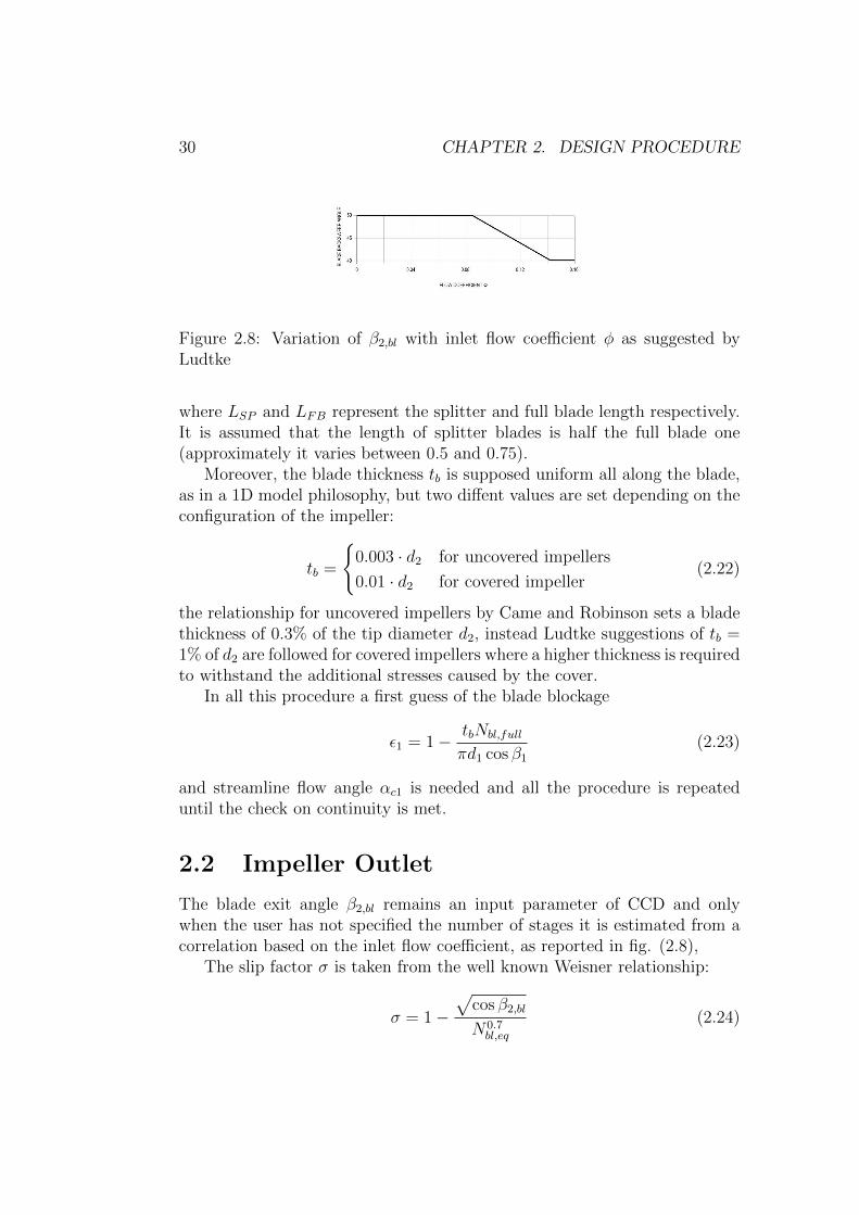
Figure 2.8: Variation of β2,bl with inlet flow coefficient φ as suggested byLudtke
where LSP and LFB represent the splitter and full blade length respectively.It is assumed that the length of splitter blades is half the full blade one(approximately it varies between 0.5 and 0.75).
Moreover, the blade thickness tb is supposed uniform all along the blade,as in a 1D model philosophy, but two diffent values are set depending on theconfiguration of the impeller:
tb =
{0.003 · d2 for uncovered impellers
0.01 · d2 for covered impeller(2.22)
the relationship for uncovered impellers by Came and Robinson sets a bladethickness of 0.3% of the tip diameter d2, instead Ludtke suggestions of tb =1% of d2 are followed for covered impellers where a higher thickness is requiredto withstand the additional stresses caused by the cover.
In all this procedure a first guess of the blade blockage
ε1 = 1− tbNbl,full
πd1 cos β1
(2.23)
and streamline flow angle αc1 is needed and all the procedure is repeateduntil the check on continuity is met.
2.2 Impeller Outlet
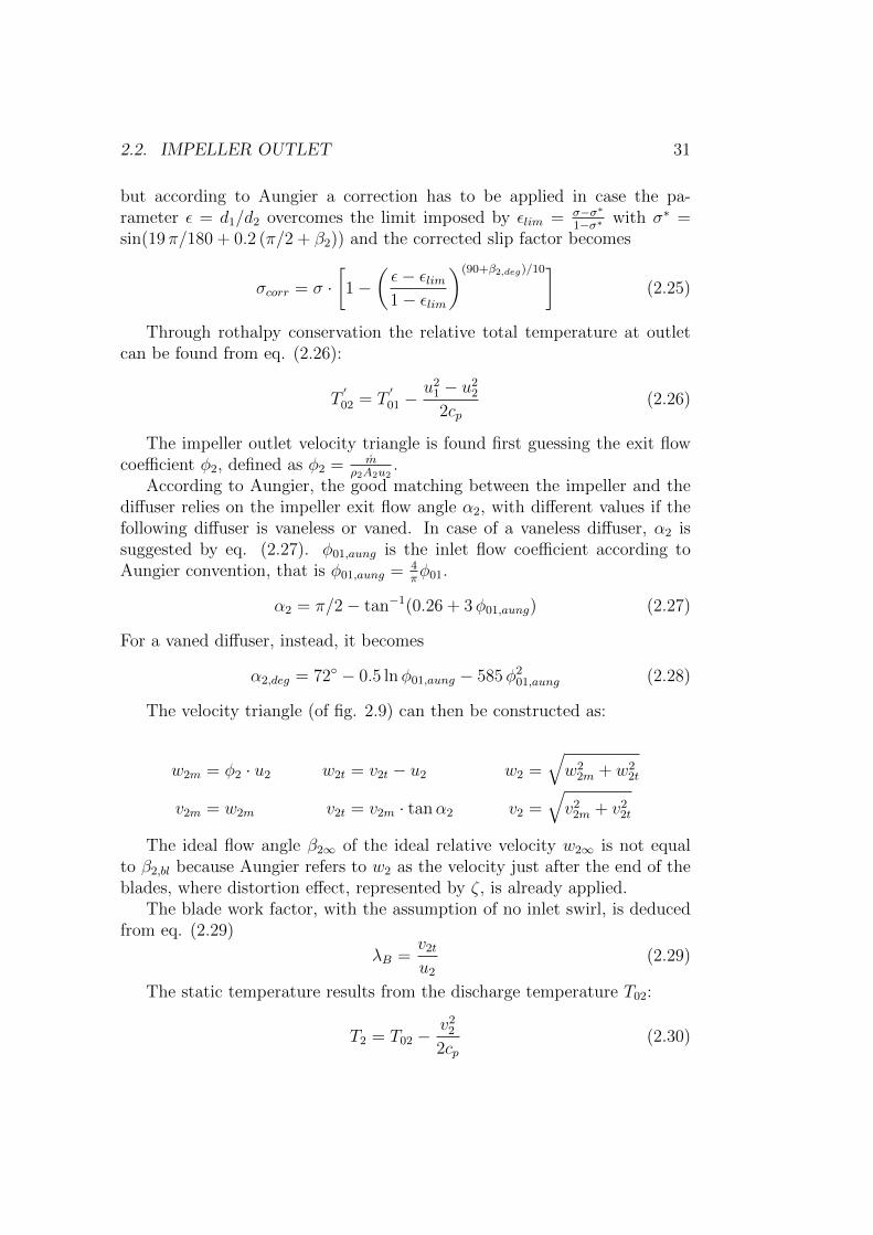
The blade exit angle β2,bl remains an input parameter of CCD and onlywhen the user has not specified the number of stages it is estimated from acorrelation based on the inlet flow coefficient, as reported in fig. (2.8),
The slip factor σ is taken from the well known Weisner relationship:
σ = 1−√
cos β2,bl
N0.7bl,eq
(2.24)
2.2. IMPELLER OUTLET 31
but according to Aungier a correction has to be applied in case the pa-rameter ε = d1/d2 overcomes the limit imposed by εlim = σ−σ∗
1−σ∗ with σ∗ =sin(19π/180 + 0.2 (π/2 + β2)) and the corrected slip factor becomes
σcorr = σ ·[1−
(ε− εlim1− εlim
)(90+β2,deg)/10](2.25)
Through rothalpy conservation the relative total temperature at outletcan be found from eq. (2.26):
T′
02 = T′
01 −u2
1 − u22
2cp(2.26)
The impeller outlet velocity triangle is found first guessing the exit flowcoefficient φ2, defined as φ2 = m
ρ2A2u2.
According to Aungier, the good matching between the impeller and thediffuser relies on the impeller exit flow angle α2, with different values if thefollowing diffuser is vaneless or vaned. In case of a vaneless diffuser, α2 issuggested by eq. (2.27). φ01,aung is the inlet flow coefficient according toAungier convention, that is φ01,aung = 4
πφ01.
α2 = π/2− tan−1(0.26 + 3φ01,aung) (2.27)
For a vaned diffuser, instead, it becomes
α2,deg = 72◦ − 0.5 lnφ01,aung − 585φ201,aung (2.28)
The velocity triangle (of fig. 2.9) can then be constructed as:
w2m = φ2 · u2 w2t = v2t − u2 w2 =√w2
2m + w22t
v2m = w2m v2t = v2m · tanα2 v2 =√v2
2m + v22t
The ideal flow angle β2∞ of the ideal relative velocity w2∞ is not equalto β2,bl because Aungier refers to w2 as the velocity just after the end of theblades, where distortion effect, represented by ζ, is already applied.
The blade work factor, with the assumption of no inlet swirl, is deducedfrom eq. (2.29)
λB =v2t
u2
(2.29)
The static temperature results from the discharge temperature T02:
T2 = T02 −v2
2
2cp(2.30)
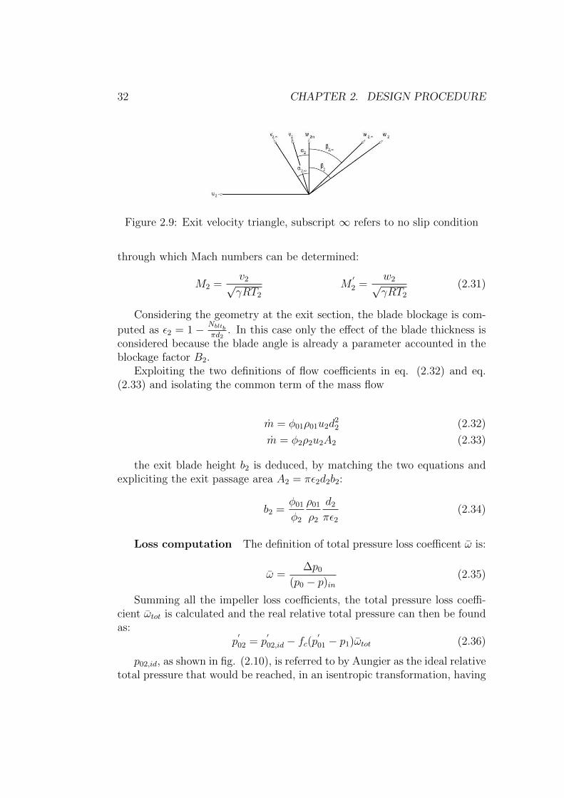
32 CHAPTER 2. DESIGN PROCEDURE
Figure 2.9: Exit velocity triangle, subscript ∞ refers to no slip condition
through which Mach numbers can be determined:
M2 =v2√γRT2
M′
2 =w2√γRT2
(2.31)
Considering the geometry at the exit section, the blade blockage is com-
puted as ε2 = 1− Nbltbπd2
. In this case only the effect of the blade thickness isconsidered because the blade angle is already a parameter accounted in theblockage factor B2.
Exploiting the two definitions of flow coefficients in eq. (2.32) and eq.(2.33) and isolating the common term of the mass flow
m = φ01ρ01u2d22 (2.32)
m = φ2ρ2u2A2 (2.33)
the exit blade height b2 is deduced, by matching the two equations andexpliciting the exit passage area A2 = πε2d2b2:
b2 =φ01
φ2
ρ01
ρ2
d2
πε2(2.34)
Loss computation The definition of total pressure loss coefficent ω is:
ω =∆p0
(p0 − p)in(2.35)
Summing all the impeller loss coefficients, the total pressure loss coeffi-cient ωtot is calculated and the real relative total pressure can then be foundas:
p′
02 = p′
02,id − fc(p′
01 − p1)ωtot (2.36)
p02,id, as shown in fig. (2.10), is referred to by Aungier as the ideal relativetotal pressure that would be reached, in an isentropic transformation, having
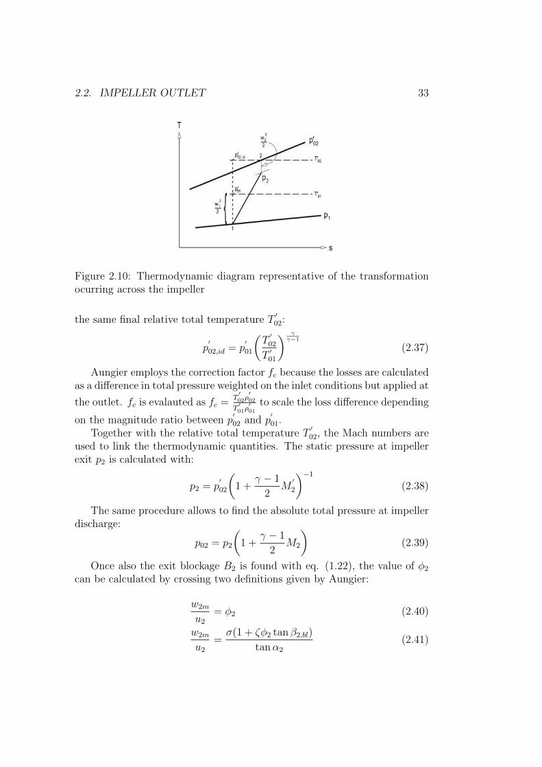
2.2. IMPELLER OUTLET 33
Figure 2.10: Thermodynamic diagram representative of the transformationocurring across the impeller
the same final relative total temperature T′02:
p′
02,id = p′
01
(T′02
T′01
) γγ−1
(2.37)
Aungier employs the correction factor fc because the losses are calculatedas a difference in total pressure weighted on the inlet conditions but applied at
the outlet. fc is evalauted as fc =T′02ρ′02
T′01ρ′01
to scale the loss difference depending
on the magnitude ratio between p′02 and p
′01.
Together with the relative total temperature T′02, the Mach numbers are
used to link the thermodynamic quantities. The static pressure at impellerexit p2 is calculated with:
p2 = p′
02
(1 +
γ − 1
2M′
2
)−1
(2.38)
The same procedure allows to find the absolute total pressure at impellerdischarge:
p02 = p2
(1 +
γ − 1
2M2
)(2.39)
Once also the exit blockage B2 is found with eq. (1.22), the value of φ2
can be calculated by crossing two definitions given by Aungier:
w2m
u2
= φ2 (2.40)
w2m
u2
=σ(1 + ζφ2 tan β2,bl)
tanα2
(2.41)
34 CHAPTER 2. DESIGN PROCEDURE
Finally, the flow coefficient φ2 can be expressed as:
φ2 =σ
tanα2 − σζ tan β2,bl
(2.42)
The parasitic losses are then computed as explained in the previous chap-ter so that the total work factor λ is recalculated with eq. (2.43):
λ = λB + λpar (2.43)
where λpar = λDF + λL + λR is the parasitic work.
2.3 Diffuser design
In a centrifugal compressor, the diffuser plays a crucial role in the recovery ofstatic pressure from the high kinetic energy stream leaving the impeller. Thiscomponent can consist in a vaneless annular space (named therefore vanelessdiffuser) or can be characterized by cascades or wedges (vaned diffuser). Onceagain, Aungier modelling has been followed both for the vaneless diffuser andthe vaned one, whose choice is set as a preference of the user in the inputfile.
2.3.1 Vaneless Diffuser
The vaneless diffuser modeled is a constant width diffuser type. Four govern-ing equations (tangential and meridional momentum, gas state and energyequation) plus some auxiliary ones are employed by Aungier to fully char-acterize the vaneless diffuser (but also more generally are valid for vanelessspaces such as also the cross over bend). The aim is to directly integratesuch equations from inlet to exit to find outlet quantities, considering whennecessary mean values along the passage. Moreover, the same perfect gasassumption made for the impeller (even if corrected for the compressibilityeffect) is kept also here. The equations are:
• Continuityπdρbvm(1−B) = m (2.44)
• Tangential momentum with friction
bvmd(rvt)
dm= −rv · vtcf (2.45)
2.3. DIFFUSER DESIGN 35
• Meridional momentum
1
ρ
dp
dm=v2t sinαCr
− vmdvmdm− cfv · vm
b− dλD
dm− λC (2.46)
• Total enthalpy
hT = h+1
2v2 (2.47)
λD and λC are two loss terms related to diffusion and curvature loss respec-tively. The diffusion loss term λD is obtainable from eq. (2.48)
dλDdm
= −2(p0 − p)(1− E)1
ρv
dv
dm(2.48)
where E represents the diffusion efficiency (its value is extrapolated from eq.(2.51)), and the curvature loss is:
λC = km(p0 − p)vm/(13ρv) (2.49)
In an annular diffuser the diffusion loss term will be predominant while ina cross-over bend the second one will. It has to be noticed that, in the radialvaneless diffuser, the infinitesimal meridional coordinate dm will become theradial coordinate dr.
Since no total pressure loss coefficients are present in this analysis, theperformance of the vaneless diffuser derives directly from the computed outletabsolute total pressure p05.
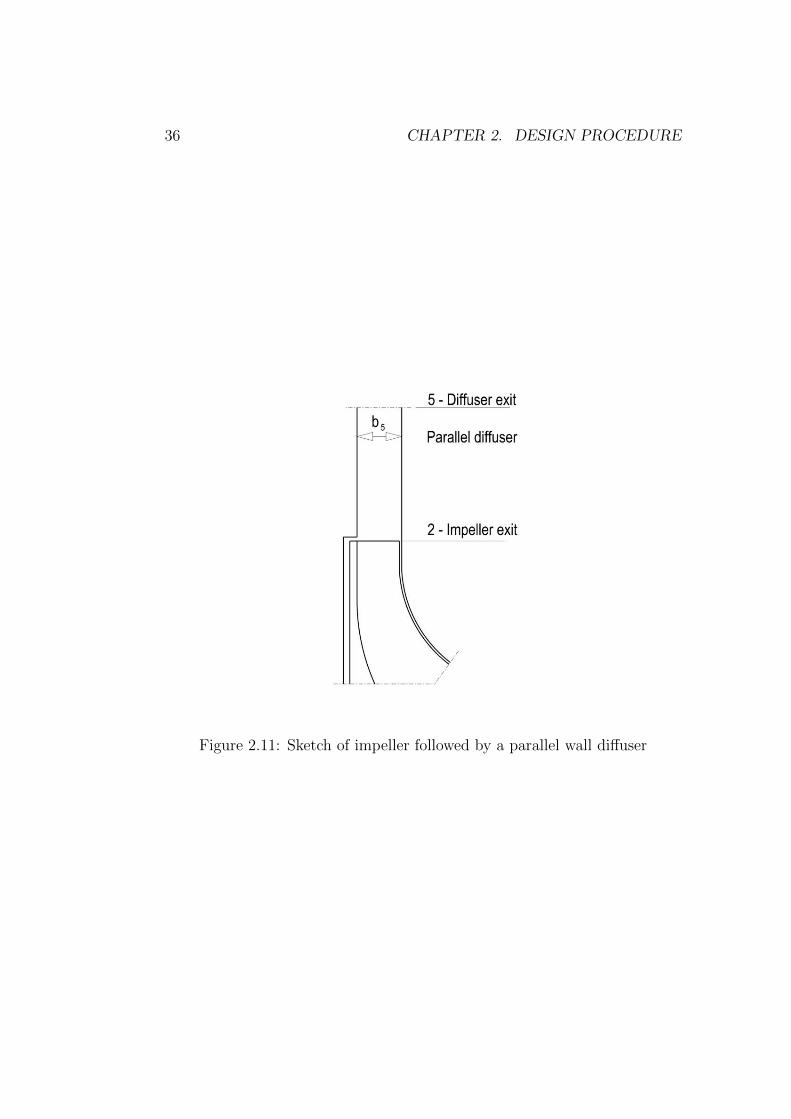
At first, a consideration has to be made: the three pivotal quantitiesin vaneless diffuser sizing are the diffuser outlet radius r5, the diffuser exitabsolute angle α5 and the passage width b5. It is important to say that itis not possible to impose a value for all of them otherwise the problem willbe over-constrained. As the walls are parallel, the width will be constant allalong the passage, so that the exit width b5 = b2. The next decision is toset the diffuser exit radius r5 so, consequentely, the diffuser outlet flow angleα5 is an output of the equations after being assumed at the beginning. Thenumerical subscripts are taken equal to the ones of the vaned diffuser wherethe exit section is station 5.
The choice of the diffuser exit radius is crucial for the effectiveness ofthis component: a too low exit radius will not lead to a satisfactory pressure
36 CHAPTER 2. DESIGN PROCEDURE
Figure 2.11: Sketch of impeller followed by a parallel wall diffuser
2.3. DIFFUSER DESIGN 37
recovery process while a too high radius will cause excessive losses due tofriction in the channel. Therefore Aungier estimates an optimal value of theexit radius r5 with eq. (2.50)
r5 =
(r5
r2
∣∣∣∣min
+4
πφ01
)r2 (2.50)
r5r2
∣∣∣∣min
represents the minimum radii ratio of the diffuser, that can be
defined in the settings file, and its typical value stands around 1.55 in order toguarantee a good operation of the diffuser. The diffuser length is L = r5− r2
and the area ratio is simply AR = r5r2
.The divergence parameter D = b2(AR − 1)/L is one of the most charac-
teristical parameters in a diffusion process. Comparing it to a reference valueDm = 0.4(b2/L)0.35, the diffusion efficiency E term is computed and used ineq. (2.48)
E =
1 when D ≤ 0
1− 0.2(D/Dm)2 when 0 < D < Dm
0.8√Dm/D when D ≥ Dm
(2.51)
Aungier uses a simple boundary layer growth model to estimate the block-age at diffuser inlet and outlet through the boundary layer thickness 2δ. Theinlet boundary layer thickness 2δin is related to impeller friction coefficent cfand blade mean camberline LB:
2δin = 5.142cfLB (2.52)
The relationship allowing to find boundary layer thickness at outlet is:
rvt = rvte[1− 2δ/(4.5b)] (2.53)
which links the edge angular momentum rvte, constant along the passage asreferred to the free stream, to the meanline angular momentum rvt. There-fore eq. (2.53) will lead to 2δout under the constraint 2δ ≤ b, since at maxi-mum 2δout equals the passage width.
Boundary layer blockage comes from eq. (2.54)
B =2δ
8b(2.54)
The procedure starts with the calculation of the tangential velocity atdiffuser exit from eq. (2.45)
v4t =r2
r4
v2t · exp(−cfL/(b4 cos α)) (2.55)
38 CHAPTER 2. DESIGN PROCEDURE
from which the meridional velocity derives.
v5m =v5t
tan α(2.56)
From eq. (2.46) the static pressure at exit p4 is calculated and so is forthe static density ρ4, with the gas equation of state p
ρ= ZRT . If continuity
at station 5 is not satisfied, a new iteration begins (with the new values ofα5 and vm5) till a satisfactory tolerance is met.
The stability of the diffuser is guaranteed by the proper selection of dif-fuser inlet flow angle α2, consequence of the good design practice suggestedby Aungier for the impeller design.
2.3.2 Vaned Diffuser
The second type of diffuser is the vaned one. As Aungier states, a vaneddiffuser can sustain higher inlet flow angles without the risk of stall thanksto the guidance of the vanes. The advantage in this case is the use of largerpassage widths to reduce the friction losses. Therefore, it is particularlysuited for low flow coefficient compressors while for high flow coefficients itloses effectiveness. On the other hand, the presence of vanes will penalizethe performances at off-design conditions, because it will impose a smallerrange of operation.
Aungier model of the vaned diffuser is again based on some pivotal param-eters, such as the area ratio AR, the divergence angle 2θC and blade loadingparameter L that will be later discussed. As done for all vaned components,flow calculations are performed at three reference sections: vane inlet, vaneexit and throat. The vaned regions, as shown in fig. (2.12), stands bewteentwo vaneles spaces, one just after the impeller and the other before the en-trance of the next component, being a volute or a return system. The firstvaneless space is usually pinched, i.e. the two walls are not parallel, whilethe second is straight.
Anugier supplies formulas for optimal vane inlet flow angle α3, whichdepends from:
α3 =
{72◦ + α2−72◦
4when α2 ≥ 72◦
72◦ when α2 < 72◦
and vane leading edge r3 refers to eq. (2.57):
r3
r2
= 1 +90− α3
360+M2
2
15(2.57)
2.3. DIFFUSER DESIGN 39
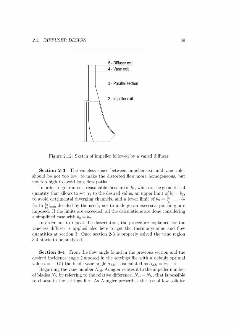
Figure 2.12: Sketch of impeller followed by a vaned diffuser
Section 2-3 The vaneless space between impeller exit and vane inletshould be not too low, to make the distorted flow more homogeneous, butnot too high to avoid long flow paths.
In order to guarantee a reasonable measure of b3, which is the geometricalquantity that allows to set α3 to the desired value, an upper limit of b3 = b2,to avoid detrimental diverging channels, and a lower limit of b3 = b3
b2|min · b2
(with b3b2|min decided by the user), not to undergo an excessive pinching, are
imposed. If the limits are exceeded, all the calculations are done consideringa simplified case with b3 = b2.
In order not to repeat the dissertation, the procedure explained for thevaneless diffuser is applied also here to get the thermodynamic and flowquantities at section 3. Once section 2-3 is properly solved the vane region3-4 starts to be analysed.
Section 3-4 From the flow angle found in the previous section and thedesired incidence angle (imposed in the settings file with a default optimalvalue i = −0.5) the blade vane angle α3,bl is calculated as α3,bl = α3 − i.
Regarding the vane number Nvd, Aungier relates it to the impeller numberof blades Nbl by referring to the relative difference, Nvd−Nbl, that is possibleto choose in the settings file. As Aungier prescribes the use of low solidity
40 CHAPTER 2. DESIGN PROCEDURE
thick vanes diffusers, Nvd will be usually lower than Nbl. Also here the vanethickness tvd is found in relative terms, with respect to inlet radius r3 andset by the designer.
The throat area calculation will be provided by some auxiliary equationsgiven by Aungier. The throat angle cosαth comes from:
cosαth = cos2 α3/ cosα3,bl (2.58)
The ideal passage throat area Ath,id follows:
Ath,id = A3 cosαth (2.59)
While the blockage is evaluated from a contraction ratio Cr calculated
using Cr =√
A3 cosα3,bl
Ath,id, indicating with A3 passage area at vane inlet. The
effective throat area can be obtained as Ath = CrAth,id from which resultsthe throat opening hth = Ath
Nvdb3.
To compute throat thermodynamic quantities the same procedure usedfor the impeller is applied also here.
The maximum extension of the blades r4,max, which is equal to vaneddiffuser outlet radius r5, follows eq. (2.50)
Three characteristic parameters for the vaned diffuser are the divergenceθC , the aforementioned area ratio AR and the blade loading L:
2θC =
2 tan−1
[(w4−tvd)b4
b3− w3 + tvd
]2LB
(2.60)
with tan θC =π(r4 cosα4,bl−r3 cosα3,bl)
LBand w4 =
2πr cosα4,bl
Nvd.
The area ratio AR here becomes:
AR =r4 cosα4,bl
r3 cosα3,bl
(2.61)
and the vane loading L
L =∆v
v3 − v4
(2.62)
where ∆v = 2π(r3Vt3−r4Vt4)NvdLB
Aungier states that the optimal ranges for these parameters are:
• 2θC7◦ < 2θC < 11◦
• AR1.4 < AR < 2.4
2.3. DIFFUSER DESIGN 41
• L0 < L < 0.33
being the upper limits for 2θC and AR the optimal values. The proceduresuggested by Aungier is to start from these best conditions and, as soon asthe constraints on r4 and L are respected, stop the analysis.
The discharge blockage factor is:
B4 =(k1 + k2(C2
R − 1))LBw4
(2.63)
with parameters:
CR =1
2
vm3 cosα4,bl
vm4 cos cosα3,bl
+ 1 (2.64)
k1 = 0.2
(1− 1
CLCθ
)(2.65)
k2 =2θC
125Cθ
(1− 2θC
22Cθ
)(2.66)
Aungier employs correction coefficients CL and Cθ in case the optimalranges of L and 2θC are not respected, as the user can modify in the settingsthe extreme limits beyond them.
Similarly to the impeller, the total pressure losses accounted for the vaneddiffuser are:
• Incidence
• Skin friction
• Mixing
• Choking
The incidence loss is found as:
ωinc = 0.8
(v3 − v3,th
v3
)2
+
(Nvdtvanes
2πr3
)2
(2.67)
Skin friction follows:
ωsf =4cf(v/v3
)2LB
dH/
(2δ
dH
)0.25
(2.68)
42 CHAPTER 2. DESIGN PROCEDURE
The mixing loss is:
ωmix =
(vm,wake − vm,mix
v3
)2
(2.69)
which comes from the same procedure applied for the impeller.
v3,sep =v3
1 + 2Cθv3,sep > v4
vm,wake =√v2sep − v2
4t v4,mix =A4vm4
2πtvdb4
And finally the choking loss:
ωch =
{0.5(0.05X +X7) if X > 0
0 if X < 0
As said for the impeller, choking occurs when CrAth = A∗ = mρ∗V ∗
.The vane angle at discharge, α4,bl, is extracted from vane length LB esti-
mation as:
cos−1
(2(r4 − r3)
LB− cosα3,bl
)(2.70)
The discharge flow angle follows Howell’s work for axial compressors:α4 = α4,bl − δ∗ − ∂δ
∂i(α3,bl − α3).
The minimum deviation angle δ∗ is:
δ∗ =
θ
(0.92
(ac
)2
+ 0.02α4,bl
)√σ − 0.02θ
(2.71)
where a/c is the maximum camber point:
a
c=
2− αbl−α3,bl
α4,bl−α3,bl
3(2.72)
The solidity σ is defined as:
σ = Nvd(r4 − r3)/(2πr3 cos αbl) (2.73)
and finally the camber θ = α4,bl − α3,bl
The variation of the deviation angle with incidence ∂δ∂i
can be computed,according to the model, as:
2.4. STAGE EXIT 43
∂δ
∂i= exp
[((1.5− 90− α3,bl
60
)2
− 3.3
)σ
](2.74)
The vane length can be approximated from eq. (2.75):
LB ∼2r3(R− 1)
cosα3,bl + cosα4,bl
(2.75)
considering the radii ratio R = r4r3
.
Once the analysis of the vanes is completed, a vaneless space with parallelwalls is supposed to be present bewteen r4 and r5, and the now well knownanalysis for vaneless spaces is followed to compute the exit flow properties.
2.4 Stage exit
The last component of a compressor stage, after the impeller and the diffuser,can consist in a volute or in a return system. They are two alternative com-ponents, meaning that they cannot be simultaneously present in the layout ofthe same stage. Usually, the return system connects stages positioned on thesame shaft while the volute is employed to bring the flow out of the machine,as required in the last stage or in intercooled stages, but the preference canbe selected in the input file.
According to Aungier, they are the two least understood and less analysedcomponents under the point of view of a 1D methodology, due to the complexflow field developing across them. Nonetheless, to consider the not negligiblelosses, a performance model and design approach have been provided by theauthor and they will be therefore used as a reference.
2.4.1 Return System
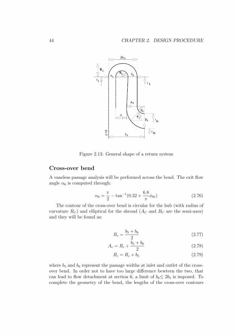
A specific routine for the return system has been implemented in Matlabcode CCD, based on the procedure reported in [1]. The return system iscomposed by two elements: the cross-over bend (a vaneless space featuringa 180◦ turn) and the return channel (a vaned region accomodating the flowto be directed into the eye of the next stage). In fig. (2.13) the shape of theconsidered return system is highlighted.
The good dimensioning suggested by Aungier means a proper scaling ofgeometric quantities, accomplished also through an optimal set of flow andblade angles.
44 CHAPTER 2. DESIGN PROCEDURE
Figure 2.13: General shape of a return system
Cross-over bend
A vaneless passage analysis will be performed across the bend. The exit flowangle α6 is computed through:
α6 =π
2− tan−1(0.32 +
6.8
πφ01) (2.76)
The contour of the cross-over bend is circular for the hub (with radius ofcurvature RC) and elliptical for the shroud (AC and BC are the semi-axes)and they will be found as:
Rc =b5 + b6
2(2.77)
Ac = Rc +b5 + b6
2(2.78)
Bc = Rc + b5 (2.79)
where b5 and b6 represent the passage widths at inlet and outlet of the cross-over bend. In order not to have too large difference bewteen the two, thatcan lead to flow detachment at section 6, a limit of b6≤ 2b5 is imposed. Tocomplete the geometry of the bend, the lengths of the cross-over contours
2.4. STAGE EXIT 45
LCO are calculated as a semi-circumference for the hub and as an arc ofellipse for the shroud:
LCO,h = πRc (2.80)
LCO,s ' π√
2(A2c +B2
c ) (2.81)
The mean streamline value for the cross-over length LCO is taken, repeat-ing what done for impeller’s inlet diameter, as a root mean square value ofthe two.
The governing equations of the vaneless space analysis, eq. (2.44) to eq.(2.47), here become:
• Tangential Momentum
bvmd(rvt)
dm= −rv · vtcf (2.82)
After integration it results:
ln
(vt6vt5
)= −cfLCO
b cos α(2.83)
• Meridional Momentum
αC is the mean streamline angle and in the cross-over bend it is nullsince αC5 = π
2and αC6 = −π
2and so sin αC = 0. Under our hypothesis
and expressing the diffusion and cruvature loss terms λD and λC , eq.(2.46) can be rewritten as:
1
γM2
dp
p=dv
vcos2 α−cf
cos α
bdm+2Z
((1+
γ − 1
2M2
) γγ−1
−1
)(1−E)
1
γM2
dv
v
−Zkm
((1 + γ−1
2M2
) γγ−1
− 1
)cos α
13γM2dm (2.84)
with passage curvature km = πLCO
Considering that∫ 6
5dm = LCO, eq. (2.84) will be integrated to find the only
unknown, that is the exit static pressure p6.v6t is gained through eq. (2.83) and with discharge flow angle also v6.
Hence, the static temperature T6 comes from eq. (2.47). Finally, the densityis calculated with the equation of state and then the passage width b6 fromcontinuity.
46 CHAPTER 2. DESIGN PROCEDURE
Return Channel
The return channel is divided in two parts: the vanes and the final turn intothe eye of the next stage. The location of mean radius r7, representing vanedischarge, is approximated by r8,s, whereas vane inclination θ at section 7 isset as a default option to θ = 45◦. Both hub and shroud contours at finalturn will be arcs of circumference. Instead, the profile of the channel betweencross-over bend and final turn is perfectly radial for the shroud while the hubone is inclined, in order to accommodate for the passage width increase asshown in fig. (2.13).
With an optimum value of incidence i indicated around 4◦, the bladeangle α6,bl can be obtained. Discharge blade angle α7,bl, instead, is imposedto 0◦. Aungier employs Howell’s deviation model for axial compressor to findthe flow angle α7, but this methodology is useful for off-design evaluation asat design point α7 = α7,bl can be assumed.
The calculation of the areas comprehends:
• Inlet area A6
A6 = 2πr6b6(1−B6,metal) (2.85)
Blade blockage B6,metal depends on the vanes number and thickness.
• Throat area Ath
Ath ≈ (2πr6 −Nvctv)b6 cosα6 (2.86)
Nvc is the vane number and tvc is the vane thickness, taken tvc = 0, 04·r6
to scale it with theradius and make the vane quite thick as consideredby Aungier and Ludtke. No aerodynamic blockage is add at exit alsobecause the thickness is considered homogeneous in this 1D approachbut at exit is thinner than at inlet.
• Exit vane area A7
A7 = (2πr7 −Nvctvc)b7 (2.87)
b7 is tha passage width at the end of the vanes.
• Return channel exit area A8
A8 = π(r28s − r2
8h) = πkr28s (2.88)
k and r8s are respectively the shape factor and the eye radius of thenext stage.

2.4. STAGE EXIT 47
Losses of Return Channel The losses are computed in terms of totalpressure loss coefficient ω based on the inlet condition at station 6
ω =p06 − p07
p06 − p6
(2.89)
• Incidence loss
ωinc = 0.8
(1− vm6
v6 cosα∗
)2
(2.90)
The optimal incidence angle α∗6 is assumed to occur when the flow inletangle is equal to the one at vane throat.
α∗6 =π
2− tan−1
[(1−B6) tan(arcsin
AthA6
)
](2.91)
indicating with B6 the aerodynamic blockage, taken as the maximumvalue between
B6 = 1− b5
b6
B6 =(kmb6)2
12 + (kmb26)
(2.92)
• Skin friction loss
ωsf = 4cf
(v
v6
)2
LB/dH +|αC6 − αC7|v6mv7m
13v26
(2.93)
dH is the hydraulic diameter found as an average between throat andvane exit and αC7 is equal to −θ.
• Blade loading loss
ωbl = (∆v/v6)2/6 (2.94)
with ∆v = 2π(r6v6t−r7v7t)NvcLB
The number of vanes Nv is obtained from a criterion that imposes theloading by fixing the velocity ratio 2∆v
v6+v7to a certain value (lower than
0.7 as recommended by Aungier) with ∆v = 2πr6v6t/(NvcLB), consid-
ering no tangential component at 7 and being LB = 2(r6−r7)cosα6,bl+cosα7,bl
the
mean camberline. It has been chosen 0.5 by default in the settings.
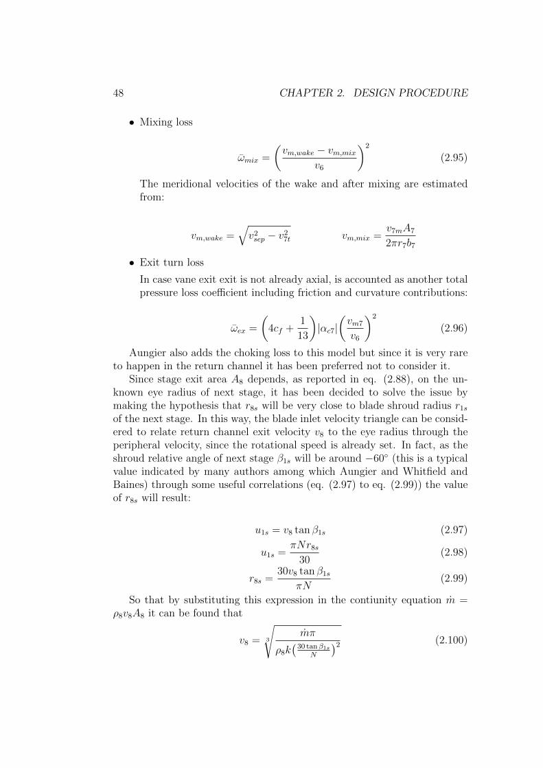
48 CHAPTER 2. DESIGN PROCEDURE
• Mixing loss
ωmix =
(vm,wake − vm,mix
v6
)2
(2.95)
The meridional velocities of the wake and after mixing are estimatedfrom:
vm,wake =√v2sep − v2
7t vm,mix =v7mA7
2πr7b7
• Exit turn loss
In case vane exit exit is not already axial, is accounted as another totalpressure loss coefficient including friction and curvature contributions:
ωex =
(4cf +
1
13
)|αc7|
(vm7
v6
)2
(2.96)
Aungier also adds the choking loss to this model but since it is very rareto happen in the return channel it has been preferred not to consider it.
Since stage exit area A8 depends, as reported in eq. (2.88), on the un-known eye radius of next stage, it has been decided to solve the issue bymaking the hypothesis that r8s will be very close to blade shroud radius r1s
of the next stage. In this way, the blade inlet velocity triangle can be consid-ered to relate return channel exit velocity v8 to the eye radius through theperipheral velocity, since the rotational speed is already set. In fact, as theshroud relative angle of next stage β1s will be around −60◦ (this is a typicalvalue indicated by many authors among which Aungier and Whitfield andBaines) through some useful correlations (eq. (2.97) to eq. (2.99)) the valueof r8s will result:
u1s = v8 tan β1s (2.97)
u1s =πNr8s
30(2.98)
r8s =30v8 tan β1s
πN(2.99)
So that by substituting this expression in the contiunity equation m =ρ8v8A8 it can be found that
v8 = 3
√mπ
ρ8k(
30 tanβ1sN
)2 (2.100)
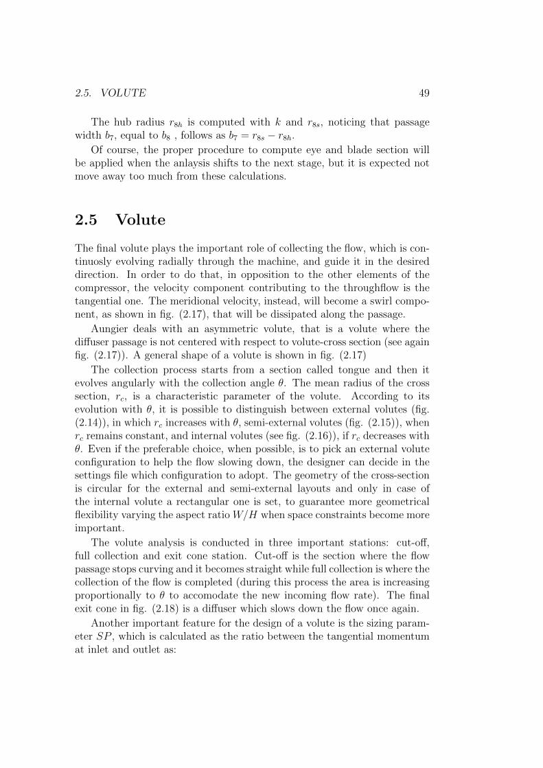
2.5. VOLUTE 49
The hub radius r8h is computed with k and r8s, noticing that passagewidth b7, equal to b8 , follows as b7 = r8s − r8h.
Of course, the proper procedure to compute eye and blade section willbe applied when the anlaysis shifts to the next stage, but it is expected notmove away too much from these calculations.
2.5 Volute
The final volute plays the important role of collecting the flow, which is con-tinuosly evolving radially through the machine, and guide it in the desireddirection. In order to do that, in opposition to the other elements of thecompressor, the velocity component contributing to the throughflow is thetangential one. The meridional velocity, instead, will become a swirl compo-nent, as shown in fig. (2.17), that will be dissipated along the passage.
Aungier deals with an asymmetric volute, that is a volute where thediffuser passage is not centered with respect to volute-cross section (see againfig. (2.17)). A general shape of a volute is shown in fig. (2.17)
The collection process starts from a section called tongue and then itevolves angularly with the collection angle θ. The mean radius of the crosssection, rc, is a characteristic parameter of the volute. According to itsevolution with θ, it is possible to distinguish between external volutes (fig.(2.14)), in which rc increases with θ, semi-external volutes (fig. (2.15)), whenrc remains constant, and internal volutes (see fig. (2.16)), if rc decreases withθ. Even if the preferable choice, when possible, is to pick an external voluteconfiguration to help the flow slowing down, the designer can decide in thesettings file which configuration to adopt. The geometry of the cross-sectionis circular for the external and semi-external layouts and only in case ofthe internal volute a rectangular one is set, to guarantee more geometricalflexibility varying the aspect ratio W/H when space constraints become moreimportant.
The volute analysis is conducted in three important stations: cut-off,full collection and exit cone station. Cut-off is the section where the flowpassage stops curving and it becomes straight while full collection is where thecollection of the flow is completed (during this process the area is increasingproportionally to θ to accomodate the new incoming flow rate). The finalexit cone in fig. (2.18) is a diffuser which slows down the flow once again.
Another important feature for the design of a volute is the sizing param-eter SP , which is calculated as the ratio between the tangential momentumat inlet and outlet as:
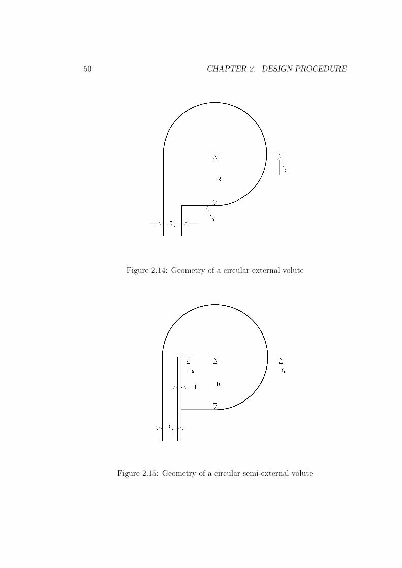
50 CHAPTER 2. DESIGN PROCEDURE
Figure 2.14: Geometry of a circular external volute
Figure 2.15: Geometry of a circular semi-external volute
2.5. VOLUTE 51
Figure 2.16: Geometry of a rectangular internal volute
Figure 2.17: General Shape of the volute
52 CHAPTER 2. DESIGN PROCEDURE
SP =r5vt5r6v6
(2.101)
It expresses the ratio of the actual volute area to the value satisfying theideal conservation of angular momentum. Typical values range from 1-1.2but also for this option the user will have the decision. SP is also employedas a correction factor to take into account distorted velocity profiles, viscouseffects and secondary flows.
In his model, Aungier considers the hypothesis of incompressible fluid(sustainable since the Mach number in this component is low) and no voluteinlet blockage. Therefore, continuity becomes:
vA(θ) = θ · (rbvm)5 (2.102)
On the contrary, in CCD density variation and diffuser exit blockageeffects are taken into account so that continuity is properly respected. Hence,eq. (2.102) becomes:
ρvA(θ) = θ · (ρrbvm)5(1−B5) (2.103)
With this approach and using the definition of SP, the cut-off area canbe calculated as:
A6,cut−off =θcut−offr6b5SPρ5(1−B5)
tanα5ρ6
(2.104)
considering a mass flow increasing linearly with the collection angle θ, A6
will be then simply found as:
A6 =2πr6b5SPρ5(1−B5)
tanα5ρ6
(2.105)
With the area varying between cut-off section and full-collection one, itis possible to keep constant the flow velocity in the passage and so alsothe tangential velocity momentum ratio because the radial coordinate is thesame.
Loss Model Aungier delivers a simple set of loss correlations both for thevolute and for the final exit cone.
• Meridional velocity loss
The coefficient corresponds to a complete loss of the meridional com-ponent
ωm =
(vm5
v5
)2
(2.106)
2.5. VOLUTE 53
• Tangential velocity loss
The loss of the tangential velocity will be dependent on the sizing pa-rameter
ωtg,vol =
0.5
r5V 2t5
r6V 25
(1− 1
SP 2
)when SP ≥ 1
r5V 2t5
r6V 25
(1− 1
SP
)2
when SP < 1
(2.107)
• Skin friction loss
Skin friction losses are directly proportional to the passage length Land inversely to the hydraulic diameter dH
ωsf = 4cf
(v6
v5
)2
L/dH (2.108)
with L = π(r5/r6)/2 and dH =√
4A6/π.
Taking advantage of the total pressure loss relationship, eq. (2.109),the total pressure at full collecton plane p06 is determined.
p06 = p05 − ωvol(p05 − p5) (2.109)
The analysis needs a guess on volute exit velocity v6 so to be able to
compute the static temperature T6 = T02 − v262cp
and the Mach number
M6 = v6√γRT6
from which the static pressure can be find:
p6 = p06
(1 +
γ − 1
2M2
)−1
(2.110)
The next step is to compute the static density with which the exitvelocity can be recalculated: v6 =
mθcut−off2πρ6A6
• Exit cone loss The exit cone loss comes from:
ωec =
(v6 − v7
v5
)2
(2.111)
The final exit cone (look at fig. (2.18)) is like an exhaust diffuserand consequently the typical diffuser parameters, such as divergenceangle 2θc, area ratio AR and length L, are used to size it. 2θc and theAR are set to optimal values if no external constraints are present, so2θc = 10, 5◦ and AR = 2.3 but also these ones are setting providedby the user. The same procedure of station 6 is then used to find thethemodynamic quantities at exit cone outlet.
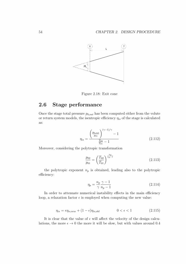
54 CHAPTER 2. DESIGN PROCEDURE
Figure 2.18: Exit cone
2.6 Stage performance
Once the stage total pressure p0,out has been computed either from the voluteor return system models, the isentropic efficiency ηis of the stage is calculatedas:
ηis =
(p0,outp01
)(γ−1)/γ
− 1
T02T01− 1
(2.112)
Moreover, considering the polytropic transformation
p02
p01
=
(T02
T01
) npnp−1
(2.113)
the polytropic exponent np is obtained, leading also to the polytropicefficiency:
ηp =npγ
γ − 1
np − 1(2.114)
In order to attenuate numerical instability effects in the main efficiencyloop, a relaxation factor ε is employed when computing the new value:
ηis = εηis,new + (1− ε)ηis,old 0 < ε < 1 (2.115)
It is clear that the value of ε will affect the velocity of the design calcu-lations, the more ε→ 0 the more it will be slow, but with values around 0.4
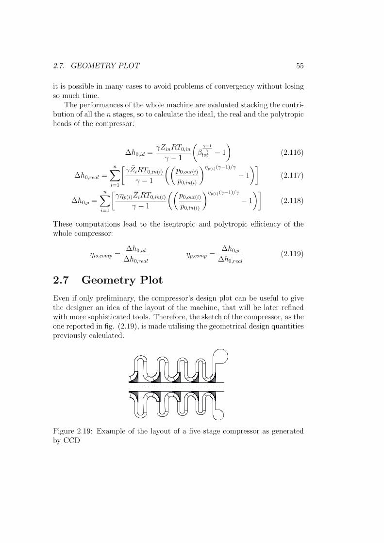
2.7. GEOMETRY PLOT 55
it is possible in many cases to avoid problems of convergency without losingso much time.
The performances of the whole machine are evaluated stacking the contri-bution of all the n stages, so to calculate the ideal, the real and the polytropicheads of the compressor:
∆h0,id =γZinRT0,in
γ − 1
(βγ−1γ
tot − 1
)(2.116)
∆h0,real =n∑i=1
[γZiRT0,in(i)
γ − 1
((p0,out(i)
p0,in(i)
)ηp(i)(γ−1)/γ
− 1
)](2.117)
∆h0,p =n∑i=1
[γηp(i)ZiRT0,in(i)
γ − 1
((p0,out(i)
p0,in(i)
)ηp(i)(γ−1)/γ
− 1
)](2.118)
These computations lead to the isentropic and polytropic efficiency of thewhole compressor:
ηis,comp =∆h0,id
∆h0,real
ηp,comp =∆h0,p
∆h0,real
(2.119)
2.7 Geometry Plot
Even if only preliminary, the compressor’s design plot can be useful to givethe designer an idea of the layout of the machine, that will be later refinedwith more sophisticated tools. Therefore, the sketch of the compressor, as theone reported in fig. (2.19), is made utilising the geometrical design quantitiespreviously calculated.
Figure 2.19: Example of the layout of a five stage compressor as generatedby CCD
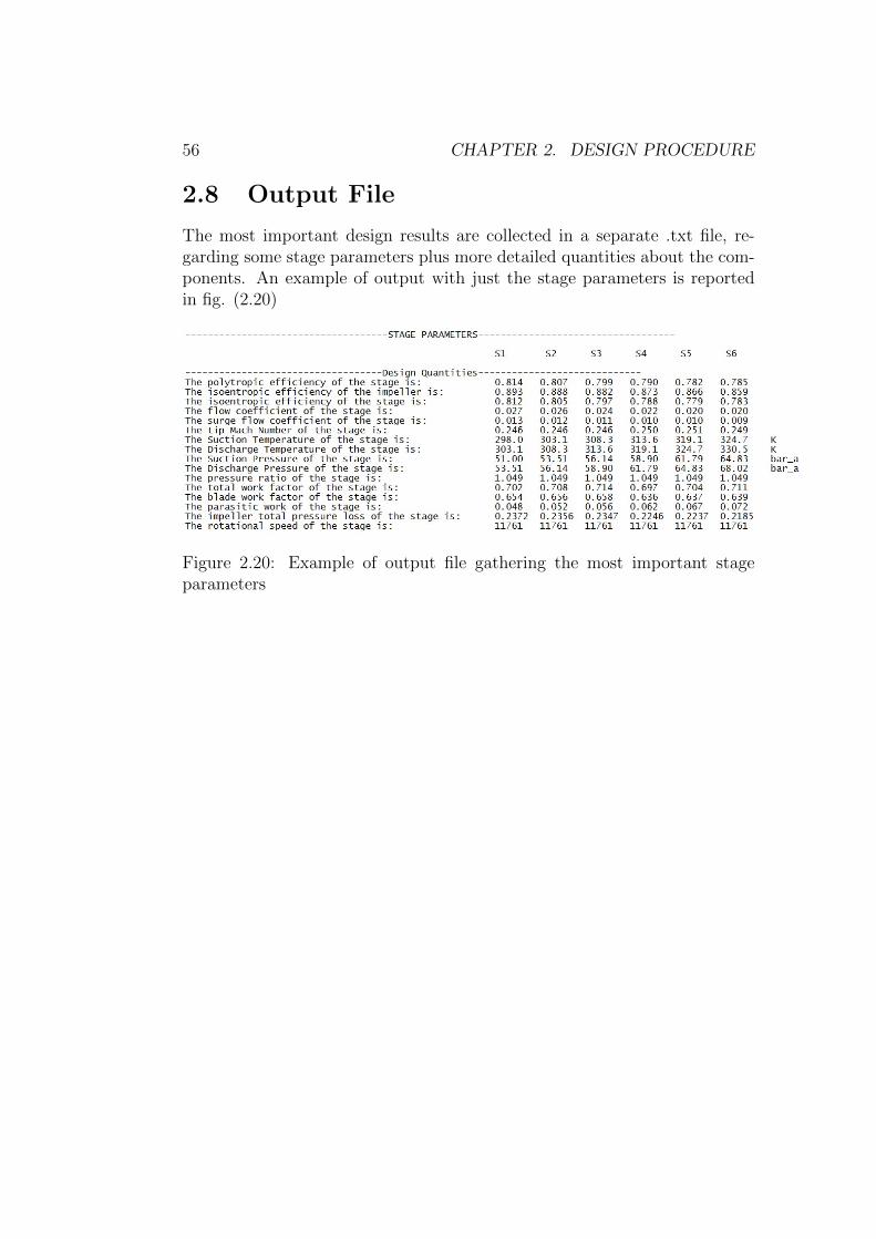
56 CHAPTER 2. DESIGN PROCEDURE
2.8 Output File
The most important design results are collected in a separate .txt file, re-garding some stage parameters plus more detailed quantities about the com-ponents. An example of output with just the stage parameters is reportedin fig. (2.20)
Figure 2.20: Example of output file gathering the most important stageparameters
Chapter 3
Off Design Performance Maps
During the preliminary design phase it is also very important, both for thedesigner and the customer, to have an idea of the off-design performances ofthe compressor in order to evaluate if the machine is suitable for the desiredapplication. The relevance of a fast and reliable estimation becomes greaterthinking of the cost and time consumption of a precise CFD analysis or of anexperimental campaign, in particular for cases where the number of stages isconsiderable.
In the recent years, a new approach has been developed and validatedby Casey and Robinson [2] for single stage compressors (then extended tomulti-stage by Al-Busaidi and Pilidis [8]), and it will be employed, as in theprevious version of CCD, to deal with the generation of the efficiency andpressure ratio maps of the compressor. The advantage is that this proceduredoes not require lots of information about the compressor and it allows aquick prediction of the performances also for multi-stage layouts.
The methodology is based on four non-dmensional parameters, the flowcoefficient φ, the efficiency η, the total work factor λ and the tip-speed Machnumber Mu2, plus some auxiliary equations and empirical parameters to becalibrated according to the specific case. Casey and Robinson motivate thechoice of these four parameters given that they are representative of somepivotal characteristics of the stage: φ referes to the type of the stage andis also somehow connected to the achievable efficiency (see the performancecharts provided in literature) as reported in Cumpsty [6], η is related tothe aerodynamic quality of the design while λ accounts for the effects of thenumber of blades and backsweep and more in general for the shape of impellerexit velcity triangle. Finally, the tip-speed Mach number Mu2 characterisesthe application of the compressor (typically process compressors have 0.5 <Mu2 < 1 and for turbochargers it can go even beyond 1.5), the ratios of totalpressures and temperatures and the effect played by compressibility.
57
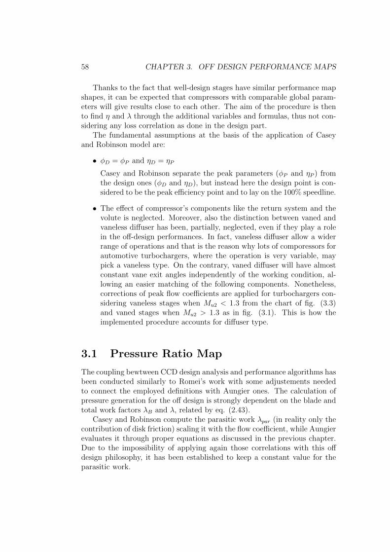
58 CHAPTER 3. OFF DESIGN PERFORMANCE MAPS
Thanks to the fact that well-design stages have similar performance mapshapes, it can be expected that compressors with comparable global param-eters will give results close to each other. The aim of the procedure is thento find η and λ through the additional variables and formulas, thus not con-sidering any loss correlation as done in the design part.
The fundamental assumptions at the basis of the application of Caseyand Robinson model are:
• φD = φP and ηD = ηP
Casey and Robinson separate the peak parameters (φP and ηP ) fromthe design ones (φD and ηD), but instead here the design point is con-sidered to be the peak efficiency point and to lay on the 100% speedline.
• The effect of compressor’s components like the return system and thevolute is neglected. Moreover, also the distinction between vaned andvaneless diffuser has been, partially, neglected, even if they play a rolein the off-design performances. In fact, vaneless diffuser allow a widerrange of operations and that is the reason why lots of comporessors forautomotive turbochargers, where the operation is very variable, maypick a vaneless type. On the contrary, vaned diffuser will have almostconstant vane exit angles independently of the working condition, al-lowing an easier matching of the following components. Nonetheless,corrections of peak flow coefficients are applied for turbochargers con-sidering vaneless stages when Mu2 < 1.3 from the chart of fig. (3.3)and vaned stages when Mu2 > 1.3 as in fig. (3.1). This is how theimplemented procedure accounts for diffuser type.
3.1 Pressure Ratio Map
The coupling bewtween CCD design analysis and performance algorithms hasbeen conducted similarly to Romei’s work with some adjustements neededto connect the employed definitions with Aungier ones. The calculation ofpressure generation for the off design is strongly dependent on the blade andtotal work factors λB and λ, related by eq. (2.43).
Casey and Robinson compute the parasitic work λpar (in reality only thecontribution of disk friction) scaling it with the flow coefficient, while Aungierevaluates it through proper equations as discussed in the previous chapter.Due to the impossibility of applying again those correlations with this offdesign philosophy, it has been established to keep a constant value for theparasitic work.
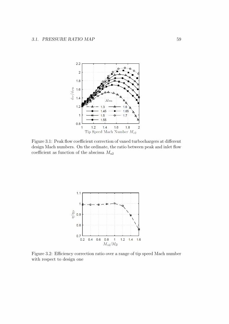
3.1. PRESSURE RATIO MAP 59
Figure 3.1: Peak flow coefficient correction of vaned turbochargers at differentdesign Mach numbers. On the ordinate, the ratio between peak and inlet flowcoefficient as function of the abscissa Mu2
Figure 3.2: Efficiency correction ratio over a range of tip speed Mach numberwith respect to design one
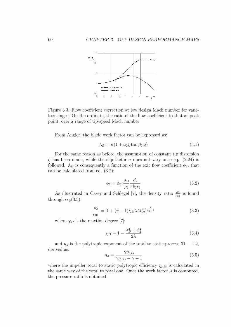
60 CHAPTER 3. OFF DESIGN PERFORMANCE MAPS
Figure 3.3: Flow coefficient correction at low design Mach number for vane-less stages. On the ordinate, the ratio of the flow coefficient to that at peakpoint, over a range of tip-speed Mach number
From Angier, the blade work factor can be expressed as:
λB = σ(1 + φ2ζ tan β2,bl) (3.1)
For the same reason as before, the assumption of constant tip distorsionζ has been made, while the slip factor σ does not vary once eq. (2.24) isfollowed. λB is consequently a function of the exit flow coefficient φ2, thatcan be calclulated from eq. (3.2):
φ2 = φ01ρ01
ρ2
d2
πb2ε2(3.2)
As illustrated in Casey and Schlegel [7], the density ratio ρ2ρ01
is found
through eq.(3.3):
ρ2
ρ01
= [1 + (γ − 1)χDλM2u2]
1nd−1 (3.3)
where χD is the reaction degree [7]:
χD = 1− λ2B + φ2
2
2λ(3.4)
and nd is the polytropic exponent of the total to static process 01 −→ 2,derived as:
nd =γηp,ts
γηp,ts − γ + 1(3.5)
where the impeller total to static polytropic efficiency ηp,ts is calculated inthe same way of the total to total one. Once the work factor λ is computed,the pressure ratio is obtained
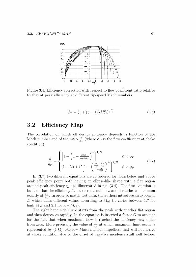
3.2. EFFICIENCY MAP 61
Figure 3.4: Efficiency correction with respect to flow coefficient ratio relativeto that at peak efficiency at different tip-speed Mach numbers
βT = (1 + (γ − 1)λM2u2)
γηpγ−1 (3.6)
3.2 Efficiency Map
The correlation on which off design efficiency depends is function of theMach number and of the ratio φ
φC(where φC is the flow coefficienct at choke
condition):
η
ηP=
[1−
(1− φ/φC
φP /φC
)D]1/D
φ < φP
(1−G) +G
[1−
(φφC−φPφC
1−φPφC
)H]1/H
φ > φP
(3.7)
In (3.7) two different equations are considered for flows below and abovepeak efficiency point both having an ellipse-like shape with a flat regionaround peak efficiency ηP , as illustrtated in fig. (3.4). The first equation isbulit so that the efficiency falls to zero at null flow and it reaches a maximumexactly at φP
φC. In order to match test data, the authors introduce an exponent
D which takes different values according to Mu2 (it varies between 1.7 forhigh Mu2 and 2.1 for low Mu2).
The right hand side curve starts from the peak with another flat regionand then decreases rapidly. In the equation is inserted a factor G to accountfor the fact that when maximum flow is reached the efficiency may differfrom zero. More precisely, the value of η
ηPat which maximum limit occur is
represented by (1-G). For low Mach number impellers, that will not arriveat choke condition due to the onset of negative incidence stall well before,
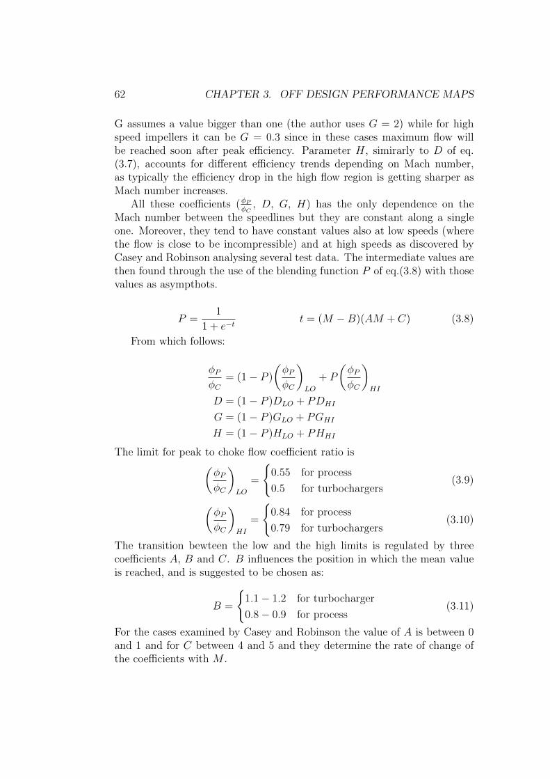
62 CHAPTER 3. OFF DESIGN PERFORMANCE MAPS
G assumes a value bigger than one (the author uses G = 2) while for highspeed impellers it can be G = 0.3 since in these cases maximum flow willbe reached soon after peak efficiency. Parameter H, simirarly to D of eq.(3.7), accounts for different efficiency trends depending on Mach number,as typically the efficiency drop in the high flow region is getting sharper asMach number increases.
All these coefficients (φPφC
, D, G, H) has the only dependence on theMach number between the speedlines but they are constant along a singleone. Moreover, they tend to have constant values also at low speeds (wherethe flow is close to be incompressible) and at high speeds as discovered byCasey and Robinson analysing several test data. The intermediate values arethen found through the use of the blending function P of eq.(3.8) with thosevalues as asympthots.
P =1
1 + e−tt = (M −B)(AM + C) (3.8)
From which follows:
φPφC
= (1− P )
(φPφC
)LO
+ P
(φPφC
)HI
D = (1− P )DLO + PDHI
G = (1− P )GLO + PGHI
H = (1− P )HLO + PHHI
The limit for peak to choke flow coefficient ratio is(φPφC
)LO
=
{0.55 for process
0.5 for turbochargers(3.9)
(φPφC
)HI
=
{0.84 for process
0.79 for turbochargers(3.10)
The transition bewteen the low and the high limits is regulated by threecoefficients A, B and C. B influences the position in which the mean valueis reached, and is suggested to be chosen as:
B =
{1.1− 1.2 for turbocharger
0.8− 0.9 for process(3.11)
For the cases examined by Casey and Robinson the value of A is between 0and 1 and for C between 4 and 5 and they determine the rate of change ofthe coefficients with M .
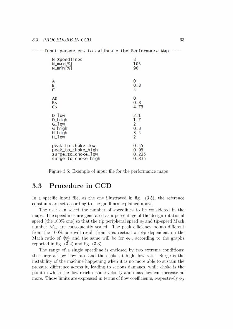
3.3. PROCEDURE IN CCD 63
Figure 3.5: Example of input file for the performance maps
3.3 Procedure in CCD
In a specific input file, as the one illustrated in fig. (3.5), the referenceconstants are set according to the guidlines explained above.
The user can select the number of speedlines to be considered in themaps. The speedlines are generated as a percentage of the design rotationalspeed (the 100% one) so that the tip peripheral speed u2 and tip-speed Machnumber Mu2 are consequently scaled. The peak efficiency points differentfrom the 100% one will result from a correction on φP dependent on theMach ratio of Mu2
MDand the same will be for φP , according to the graphs
reported in fig. (3.2) and fig. (3.3).
The range of a single speedline is enclosed by two extreme conditions:the surge at low flow rate and the choke at high flow rate. Surge is theinstability of the machine happening when it is no more able to sustain thepressure difference across it, leading to serious damages, while choke is thepoint in which the flow reaches sonic velocity and mass flow can increase nomore. Those limits are expressed in terms of flow coefficients, respectively φS
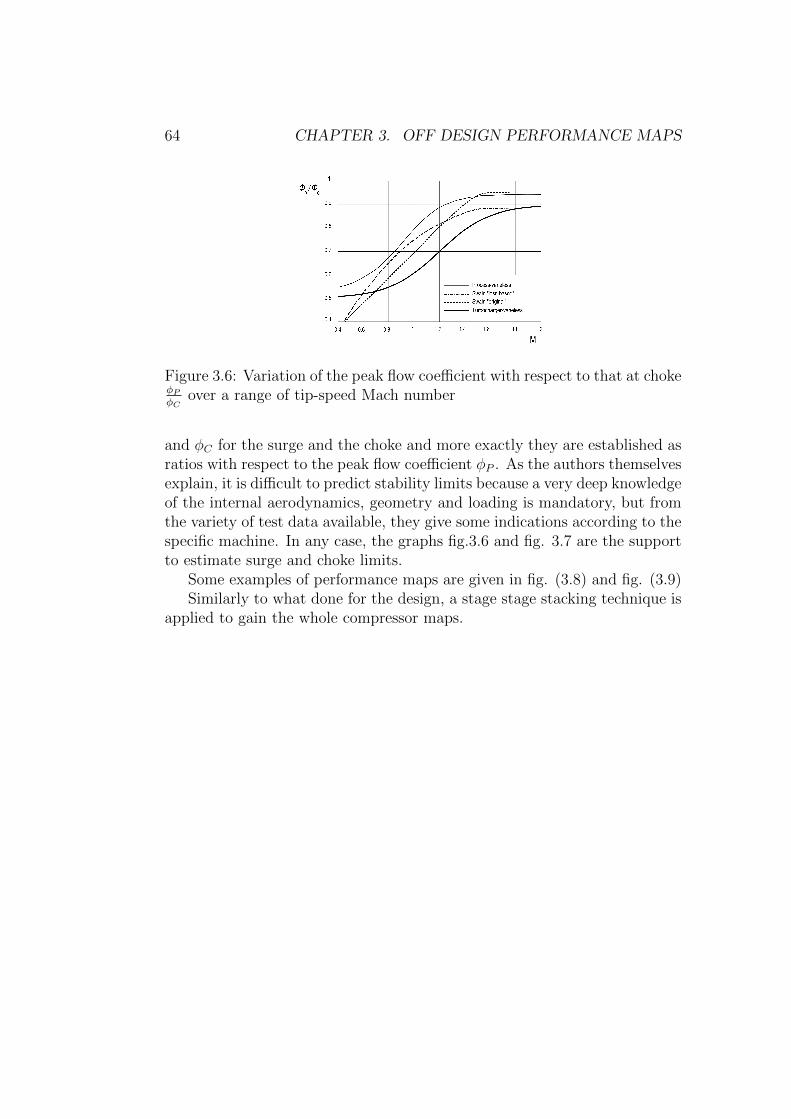
64 CHAPTER 3. OFF DESIGN PERFORMANCE MAPS
Figure 3.6: Variation of the peak flow coefficient with respect to that at chokeφPφC
over a range of tip-speed Mach number
and φC for the surge and the choke and more exactly they are established asratios with respect to the peak flow coefficient φP . As the authors themselvesexplain, it is difficult to predict stability limits because a very deep knowledgeof the internal aerodynamics, geometry and loading is mandatory, but fromthe variety of test data available, they give some indications according to thespecific machine. In any case, the graphs fig.3.6 and fig. 3.7 are the supportto estimate surge and choke limits.
Some examples of performance maps are given in fig. (3.8) and fig. (3.9)Similarly to what done for the design, a stage stage stacking technique is
applied to gain the whole compressor maps.
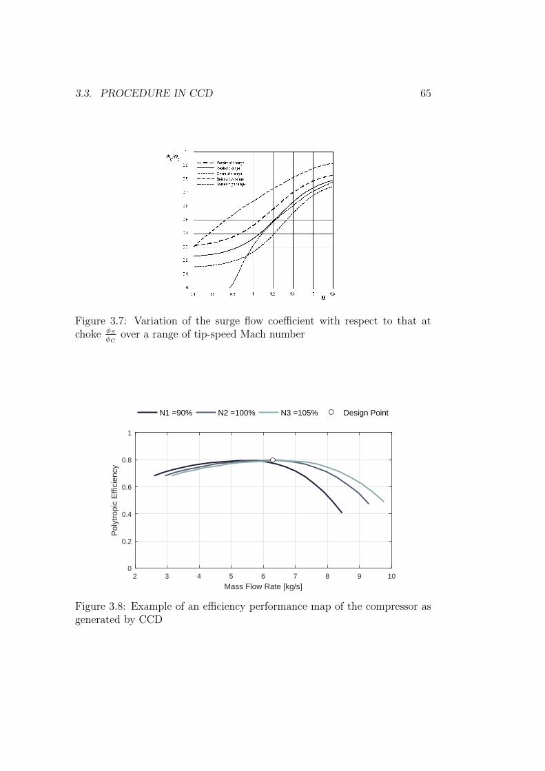
3.3. PROCEDURE IN CCD 65
Figure 3.7: Variation of the surge flow coefficient with respect to that atchoke φS
φCover a range of tip-speed Mach number
2 3 4 5 6 7 8 9 10
Mass Flow Rate [kg/s]
0
0.2
0.4
0.6
0.8
1
Pol
ytro
pic
Effi
cien
cy
N1 =90% N2 =100% N3 =105% Design Point
Figure 3.8: Example of an efficiency performance map of the compressor asgenerated by CCD
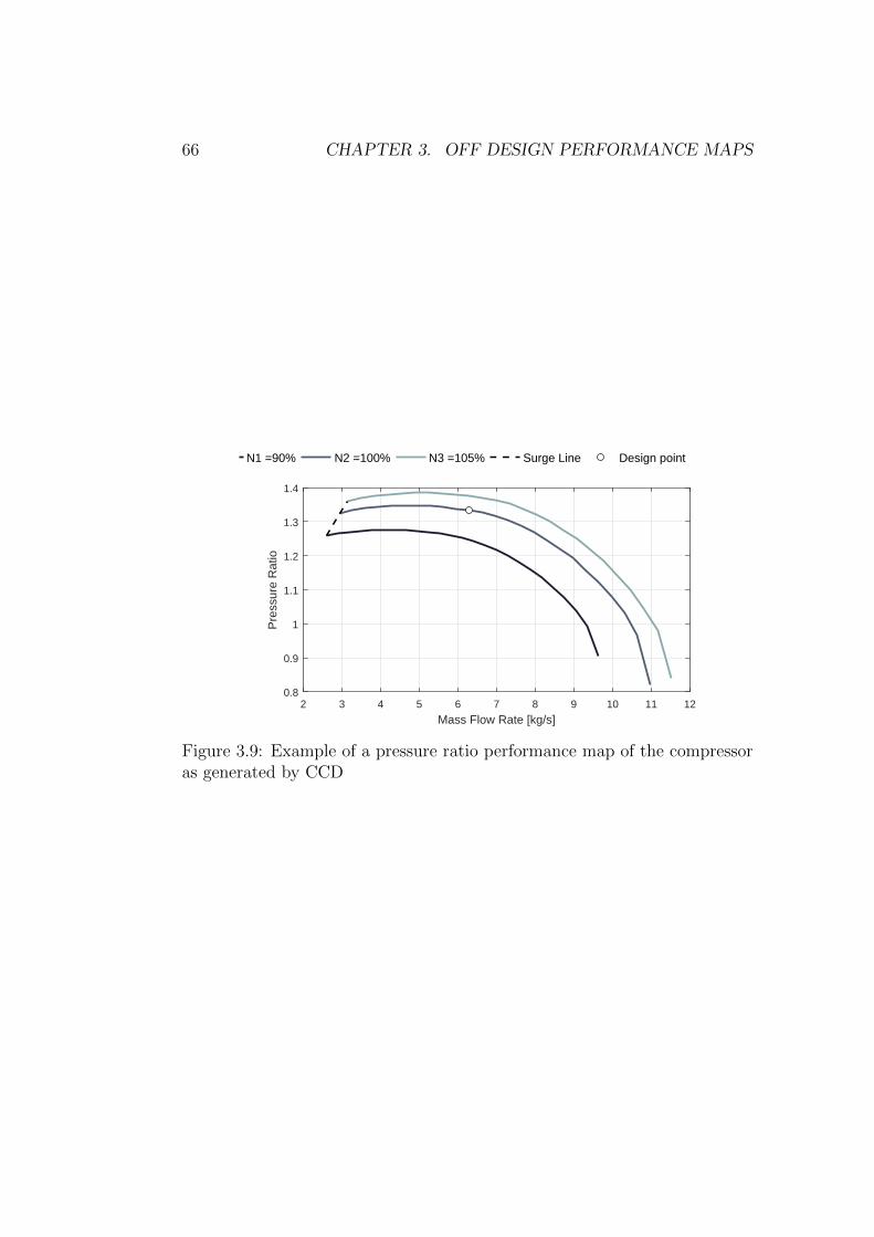
66 CHAPTER 3. OFF DESIGN PERFORMANCE MAPS
2 3 4 5 6 7 8 9 10 11 12
Mass Flow Rate [kg/s]
0.8
0.9
1
1.1
1.2
1.3
1.4
Pre
ssur
e R
atio
N1 =90% N2 =100% N3 =105% Surge Line Design point
Figure 3.9: Example of a pressure ratio performance map of the compressoras generated by CCD
Chapter 4
Validation
In this chapter the application and validation of the new implemented codeis discussed.
In order to compare both the preliminary design quantities and the peakperformances, looking also at the off-design behaviour, four test cases havebeen considered:
• 3 Stage compressor - IGCC (Integrally Geared Centrifugal Compressor)
• 5 stage compressor - process
• 6 stage compressor - hydrogen rich gas
• 1 stage compressor - turbocharger HECC (High Efficiency CentrifugalCompressor)
It has to be pointed out that the validation process is made more difficultby the fact that no complete information about the compressors is usuallyavailable in open literature. In fact, it is common to find quite detaileddescriptions about the design of a compressor with just a hint on the perfor-mance maps and viceversa; the consequence is that some parameters mustbe reasonably guessed in order to perform the simulations.
First of all, in order not to confuse the reader, the version of CCD whichis currently discussed in this thesis is named CCD V03, since two versions,CCD V01 and CCD V02, were created by A. Romei in his work, differing inthe philosphy for blade exit angle β2,bl computation. The comparisons willbe made with CCD V01 as, like in CCD V03, the possibility of selecting β2,bl
is given in the input file, allowing a more proper procedure.The choice of these particular validation cases has been made considering
that the first three have been analysed also for CCD V01 and it was a due
67
68 CHAPTER 4. VALIDATION
benchmark, while the last one has been added mainly because some CFDstudies at the Von Karman Institute have been conducted about it and acomprehensive paper was published on its regard.
The adopted strategy is to confront the obtained results of the new CCDV03 both with the test data and with CCD V01. At first, the same inputemployed at its time for CCD V01 is used to examine what the outcome iswhen equal information are provided. Successively, if necessary, some inputparameters are tuned to catch more precisely important characteristics of thetest cases.
4.1 3 stages IGCC
In the recent years, the applications with integrally geared centrifugal com-pressor (IGCC) have been continuously increasing, from air separation plantsto power generation and hydrocarbon refrigeration. An IGCC is an efficientand reliable multi-shaft machine in which a proper gear coupling intercon-nects the shafts regulating the rotational speeds [9]. The removal of thevelocity constraint and the possibility of employing intercoolers are the mostremarkable advantages that make this arrangement frequently preferable toin-line compressors.
The present IGCC is a 3 stages machine working with air. The stages aremounted on two shafts: two stages on the first shaft, both with intercoolers,and the third stage on the other, that is the fastest. Moreover, the first stageis equppied with a vaned diffuser while the others with a vaneless one. Apicture of the geometry as generated by CCD is illustrated in fig. (4.1).
Since, for this case, geometrical and performance data have been reach-able [12], a careful analysis has been made. Table 4.1 reports the comparisonbetween CCD V03 and the test data, with the indication of the relative er-rors between the two, calculated as
(XCCD−Xref
)/Xref , where X indicates
a general compressor quantity. The same comparison, but with respect tothe results of CCD V01, is done in table 4.2.
Tables 4.1 and 4.2 higlight that the the thermodynamic outlet quantitiesof the stages are well foreseen by the code (the relative errors are all less than1%), thanks also to the role played by the intercoolers, that impose fix suctiontemperatures for both the second and the last stage, reducing possible errorsaccumulation from one stage to another. In general, the second stage is theone that distances itself the most from the reference compressors parameterssuch as tip speed Mach number Mu2 (deviation of −4%) and total work factorλ (deviation of +8.2%). The cause can be found in the lower estimationof both the rotational speed and tip diameter. On the contrary, the peak
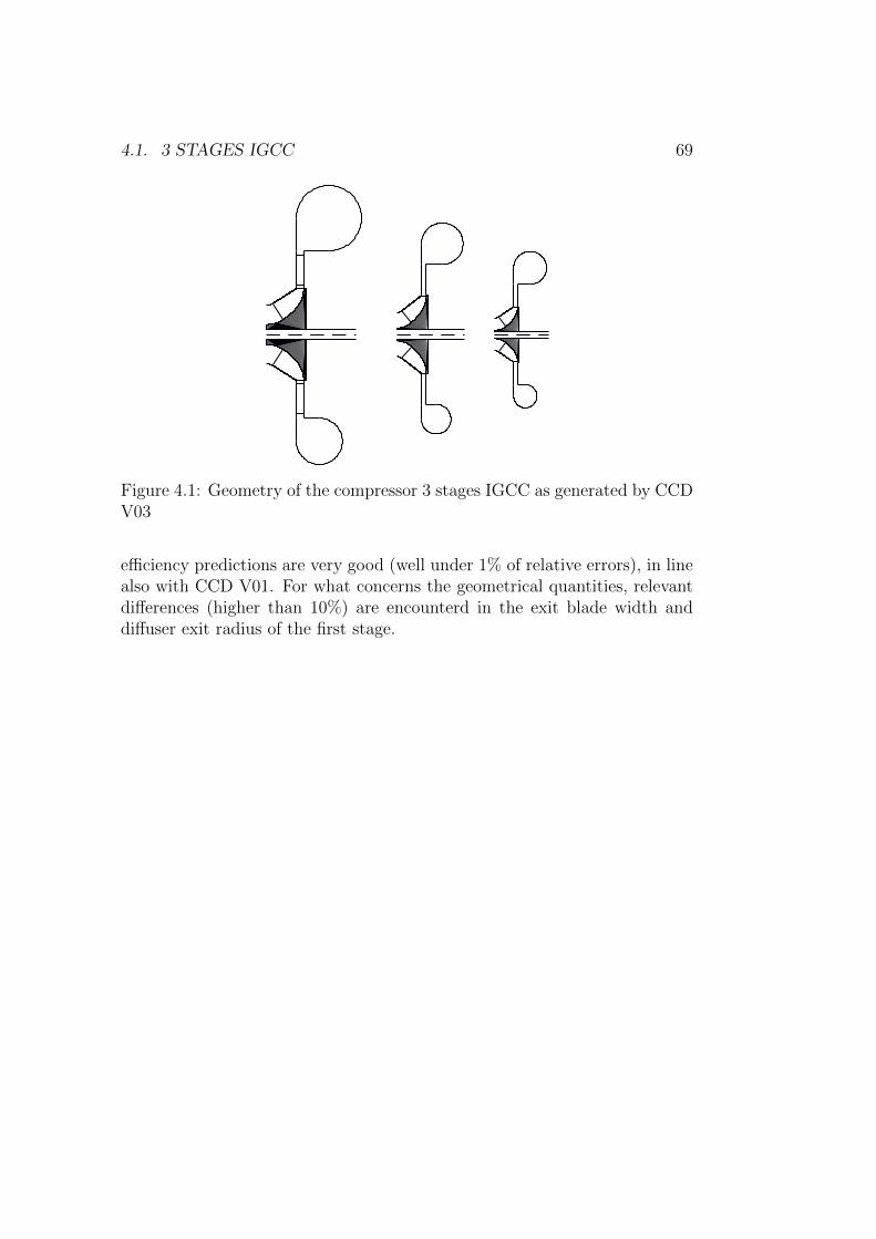
4.1. 3 STAGES IGCC 69
Figure 4.1: Geometry of the compressor 3 stages IGCC as generated by CCDV03
efficiency predictions are very good (well under 1% of relative errors), in linealso with CCD V01. For what concerns the geometrical quantities, relevantdifferences (higher than 10%) are encounterd in the exit blade width anddiffuser exit radius of the first stage.
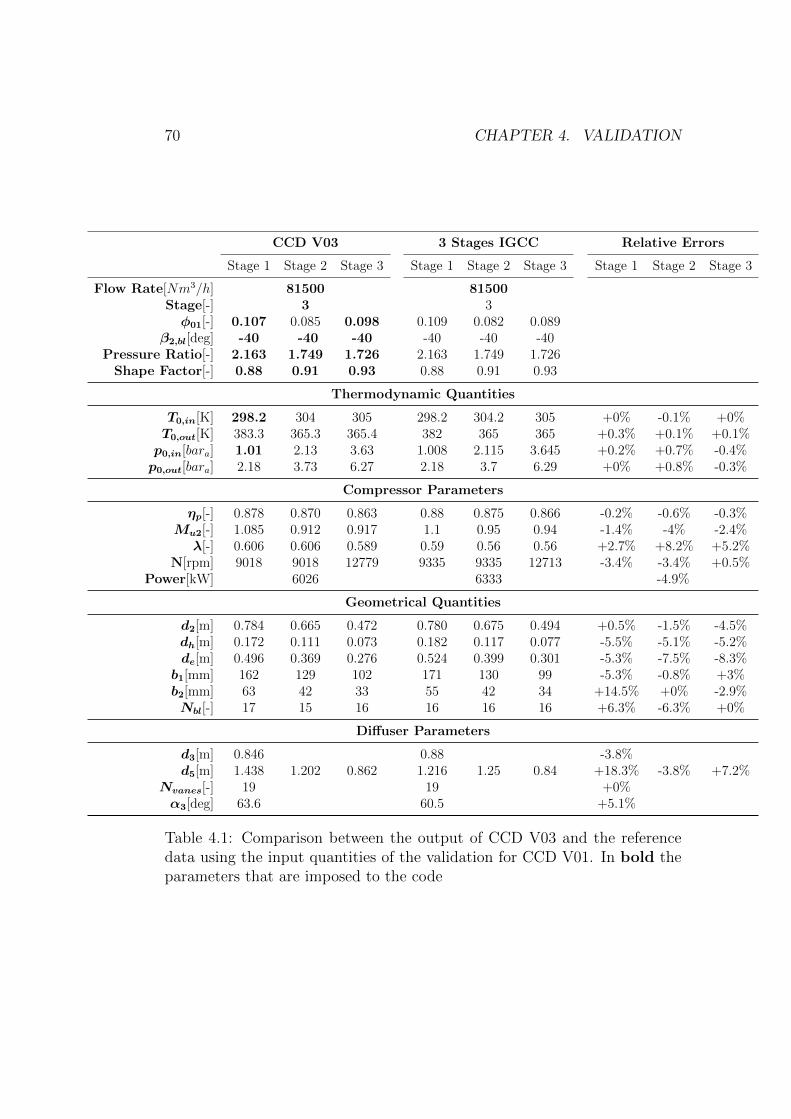
70 CHAPTER 4. VALIDATION
CCD V03 3 Stages IGCC Relative Errors
Stage 1 Stage 2 Stage 3 Stage 1 Stage 2 Stage 3 Stage 1 Stage 2 Stage 3
Flow Rate[Nm3/h] 81500 81500Stage[-] 3 3φ01[-] 0.107 0.085 0.098 0.109 0.082 0.089
β2,bl[deg] -40 -40 -40 -40 -40 -40Pressure Ratio[-] 2.163 1.749 1.726 2.163 1.749 1.726
Shape Factor[-] 0.88 0.91 0.93 0.88 0.91 0.93
Thermodynamic Quantities
T0,in[K] 298.2 304 305 298.2 304.2 305 +0% -0.1% +0%T0,out[K] 383.3 365.3 365.4 382 365 365 +0.3% +0.1% +0.1%p0,in[bara] 1.01 2.13 3.63 1.008 2.115 3.645 +0.2% +0.7% -0.4%p0,out[bara] 2.18 3.73 6.27 2.18 3.7 6.29 +0% +0.8% -0.3%
Compressor Parameters
ηp[-] 0.878 0.870 0.863 0.88 0.875 0.866 -0.2% -0.6% -0.3%Mu2[-] 1.085 0.912 0.917 1.1 0.95 0.94 -1.4% -4% -2.4%λ[-] 0.606 0.606 0.589 0.59 0.56 0.56 +2.7% +8.2% +5.2%
N[rpm] 9018 9018 12779 9335 9335 12713 -3.4% -3.4% +0.5%Power[kW] 6026 6333 -4.9%
Geometrical Quantities
d2[m] 0.784 0.665 0.472 0.780 0.675 0.494 +0.5% -1.5% -4.5%dh[m] 0.172 0.111 0.073 0.182 0.117 0.077 -5.5% -5.1% -5.2%de[m] 0.496 0.369 0.276 0.524 0.399 0.301 -5.3% -7.5% -8.3%b1[mm] 162 129 102 171 130 99 -5.3% -0.8% +3%b2[mm] 63 42 33 55 42 34 +14.5% +0% -2.9%Nbl[-] 17 15 16 16 16 16 +6.3% -6.3% +0%
Diffuser Parameters
d3[m] 0.846 0.88 -3.8%d5[m] 1.438 1.202 0.862 1.216 1.25 0.84 +18.3% -3.8% +7.2%
Nvanes[-] 19 19 +0%α3[deg] 63.6 60.5 +5.1%
Table 4.1: Comparison between the output of CCD V03 and the referencedata using the input quantities of the validation for CCD V01. In bold theparameters that are imposed to the code
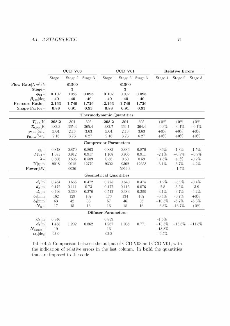
4.1. 3 STAGES IGCC 71
CCD V03 CCD V01 Relative Errors
Stage 1 Stage 2 Stage 3 Stage 1 Stage 2 Stage 3 Stage 1 Stage 2 Stage 3
Flow Rate[Nm3/h] 81500 81500Stage[-] 3 3φ01[-] 0.107 0.085 0.098 0.107 0.092 0.098
β2,bl[deg] -40 -40 -40 -40 -40 -40Pressure Ratio[-] 2.163 1.749 1.726 2.163 1.749 1.726
Shape Factor[-] 0.88 0.91 0.93 0.88 0.91 0.93
Thermodynamic Quantities
T0,in[K] 298.2 304 305 298.2 304 305 +0% +0% +0%T0,out[K] 383.3 365.3 365.4 382.7 364.1 364.4 +0.3% +0.1% +0.1%p0,in[bara] 1.01 2.13 3.63 1.01 2.13 3.63 +0% +0% +0%p0,out[bara] 2.18 3.73 6.27 2.18 3.73 6.27 +0% +0% +0%
Compressor Parameters
ηp[-] 0.878 0.870 0.863 0.883 0.886 0.876 -0.6% -1.8% -1.5%Mu2[-] 1.085 0.912 0.917 1.108 0.905 0.911 -2.1% +0.8% +0.7%λ[-] 0.606 0.606 0.589 0.58 0.60 0.59 +4.5% +1% -0.2%
N[rpm] 9018 9018 12779 9302 9302 12653 -3.1% -3.7% -4.2%Power[kW] 6026 5964.3 +1.5%
Geometrical Quantities
d2[m] 0.784 0.665 0.472 0.775 0.640 0.474 +1.2% +3.9% -0.4%dh[m] 0.172 0.111 0.73 0.177 0.115 0.076 -2.8 -3.5% -3.9de[m] 0.496 0.369 0.276 0.512 0.383 0.288 -3.1% -3.7% -4.2%b1[mm] 162 129 102 173 134 102 -6.4% -3.7% +0%b2[mm] 63 42 33 57 46 36 +10.5% -8.7% -8.3%Nbl[-] 17 15 16 16 18 16 +6.3% -16.7% +0%
Diffuser Parameters
d3[m] 0.846 0.859 -1.5%d5[m] 1.438 1.202 0.862 1.267 1.038 0.771 +13.5% +15.8% +11.8%
Nvanes[-] 19 16 +18.8%α3[deg] 63.6 63.3 +0.5%
Table 4.2: Comparison between the output of CCD V03 and CCD V01, withthe indication of relative errors in the last column. In bold the quantitiesthat are imposed to the code
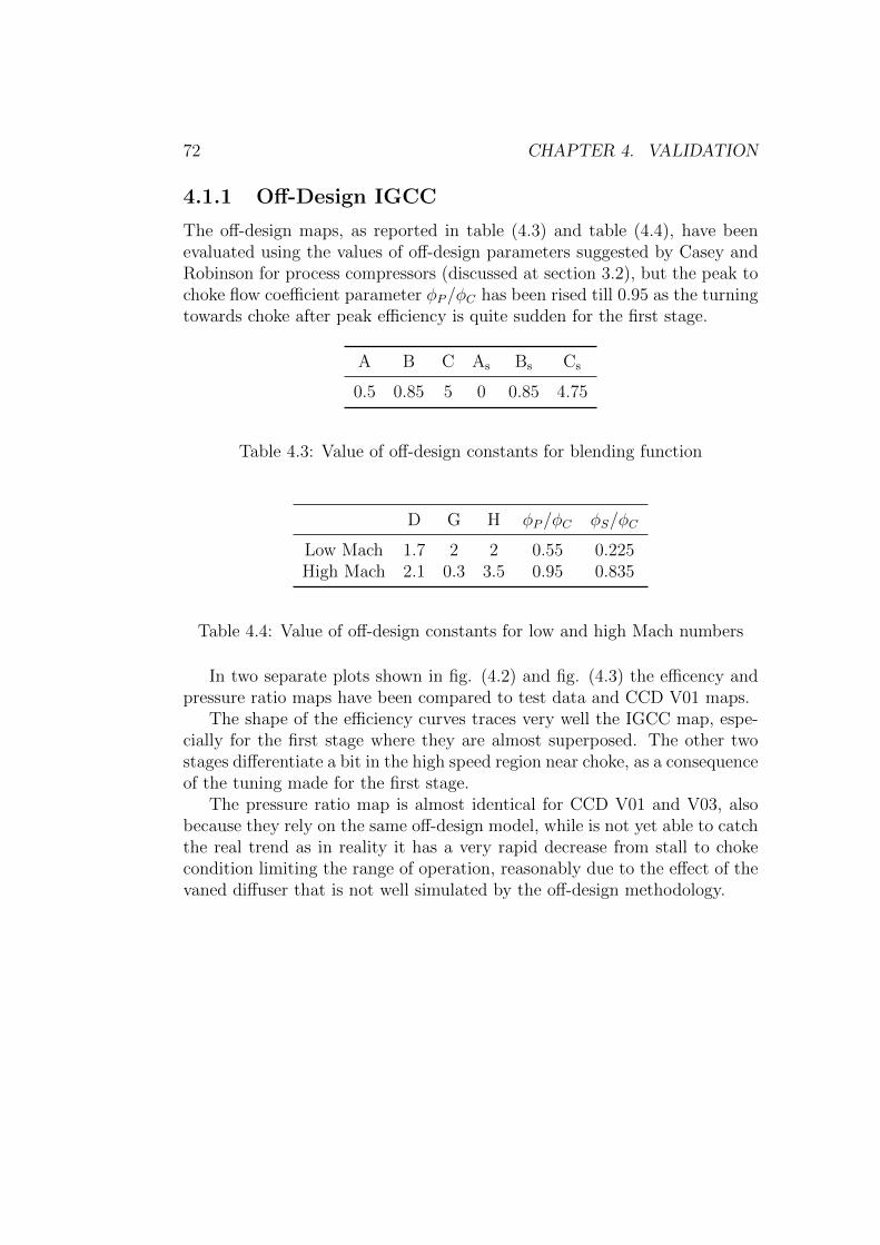
72 CHAPTER 4. VALIDATION
4.1.1 Off-Design IGCC
The off-design maps, as reported in table (4.3) and table (4.4), have beenevaluated using the values of off-design parameters suggested by Casey andRobinson for process compressors (discussed at section 3.2), but the peak tochoke flow coefficient parameter φP/φC has been rised till 0.95 as the turningtowards choke after peak efficiency is quite sudden for the first stage.
A B C As Bs Cs
0.5 0.85 5 0 0.85 4.75
Table 4.3: Value of off-design constants for blending function
D G H φP/φC φS/φC
Low Mach 1.7 2 2 0.55 0.225High Mach 2.1 0.3 3.5 0.95 0.835
Table 4.4: Value of off-design constants for low and high Mach numbers
In two separate plots shown in fig. (4.2) and fig. (4.3) the efficency andpressure ratio maps have been compared to test data and CCD V01 maps.
The shape of the efficiency curves traces very well the IGCC map, espe-cially for the first stage where they are almost superposed. The other twostages differentiate a bit in the high speed region near choke, as a consequenceof the tuning made for the first stage.
The pressure ratio map is almost identical for CCD V01 and V03, alsobecause they rely on the same off-design model, while is not yet able to catchthe real trend as in reality it has a very rapid decrease from stall to chokecondition limiting the range of operation, reasonably due to the effect of thevaned diffuser that is not well simulated by the off-design methodology.
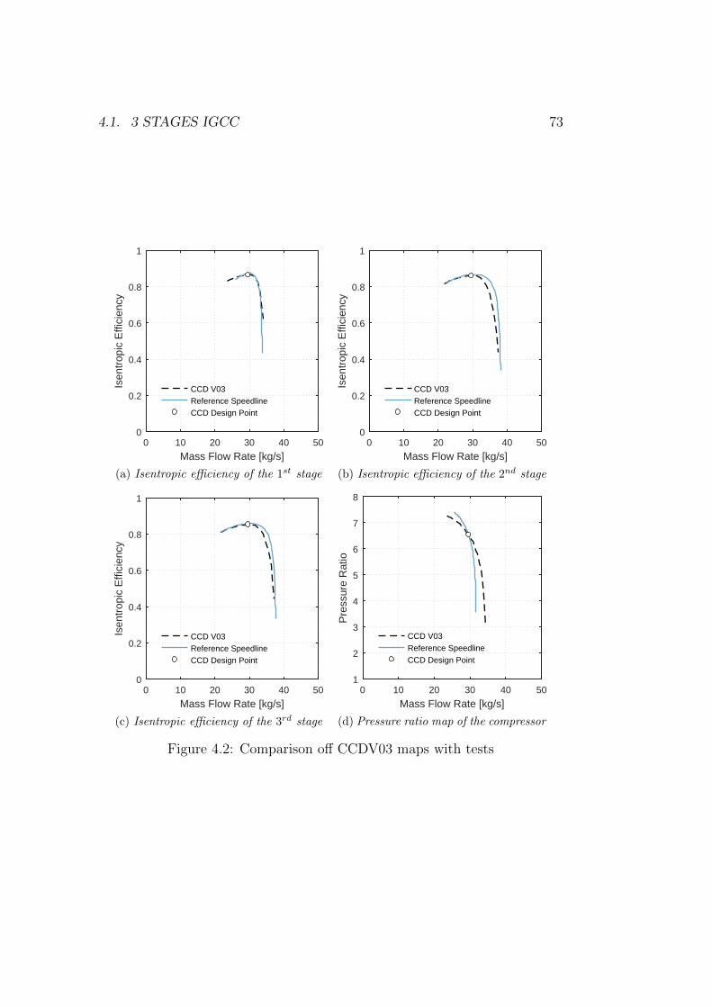
4.1. 3 STAGES IGCC 73
0 10 20 30 40 50
Mass Flow Rate [kg/s]
0
0.2
0.4
0.6
0.8
1
Isen
trop
ic E
ffici
ency
CCD V03Reference SpeedlineCCD Design Point
(a) Isentropic efficiency of the 1st stage
0 10 20 30 40 50
Mass Flow Rate [kg/s]
0
0.2
0.4
0.6
0.8
1
Isen
trop
ic E
ffici
ency
CCD V03Reference SpeedlineCCD Design Point
(b) Isentropic efficiency of the 2nd stage
0 10 20 30 40 50
Mass Flow Rate [kg/s]
0
0.2
0.4
0.6
0.8
1
Isen
trop
ic E
ffici
ency
CCD V03Reference SpeedlineCCD Design Point
(c) Isentropic efficiency of the 3rd stage
0 10 20 30 40 50
Mass Flow Rate [kg/s]
1
2
3
4
5
6
7
8
Pre
ssur
e R
atio
CCD V03Reference SpeedlineCCD Design Point
(d) Pressure ratio map of the compressor
Figure 4.2: Comparison off CCDV03 maps with tests
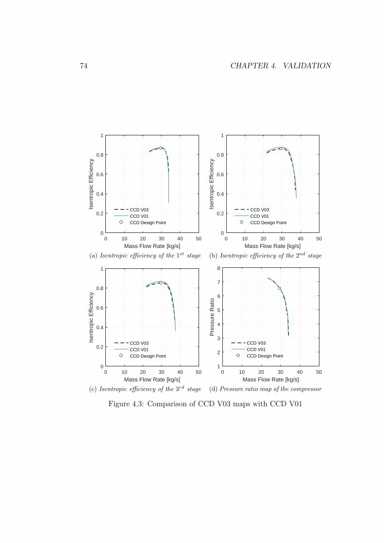
74 CHAPTER 4. VALIDATION
0 10 20 30 40 50
Mass Flow Rate [kg/s]
0
0.2
0.4
0.6
0.8
1
Isen
trop
ic E
ffici
ency
CCD V03CCD V01CCD Design Point
(a) Isentropic efficiency of the 1st stage
0 10 20 30 40 50
Mass Flow Rate [kg/s]
0
0.2
0.4
0.6
0.8
1
Isen
trop
ic E
ffici
ency
CCD V03CCD V01CCD Design Point
(b) Isentropic efficiency of the 2nd stage
0 10 20 30 40 50
Mass Flow Rate [kg/s]
0
0.2
0.4
0.6
0.8
1
Isen
trop
ic E
ffici
ency
CCD V03CCD V01CCD Design Point
(c) Isentropic efficiency of the 3rd stage
0 10 20 30 40 50
Mass Flow Rate [kg/s]
1
2
3
4
5
6
7
8
Pre
ssur
e R
atio
CCD V03CCD V01CCD Design Point
(d) Pressure ratio map of the compressor
Figure 4.3: Comparison of CCD V03 maps with CCD V01
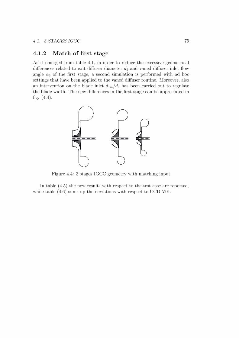
4.1. 3 STAGES IGCC 75
4.1.2 Match of first stage
As it emerged from table 4.1, in order to reduce the excessive geometricaldifferences related to exit diffuser diameter d5 and vaned diffuser inlet flowangle α3 of the first stage, a second simulation is performed with ad hocsettings that have been applied to the vaned diffuser routine. Moreover, alsoan intervention on the blade inlet d1m/de has been carried out to regulatethe blade width. The new differences in the first stage can be appreciated infig. (4.4).
Figure 4.4: 3 stages IGCC geometry with matching input
In table (4.5) the new results with respect to the test case are reported,while table (4.6) sums up the deviations with respect to CCD V01.
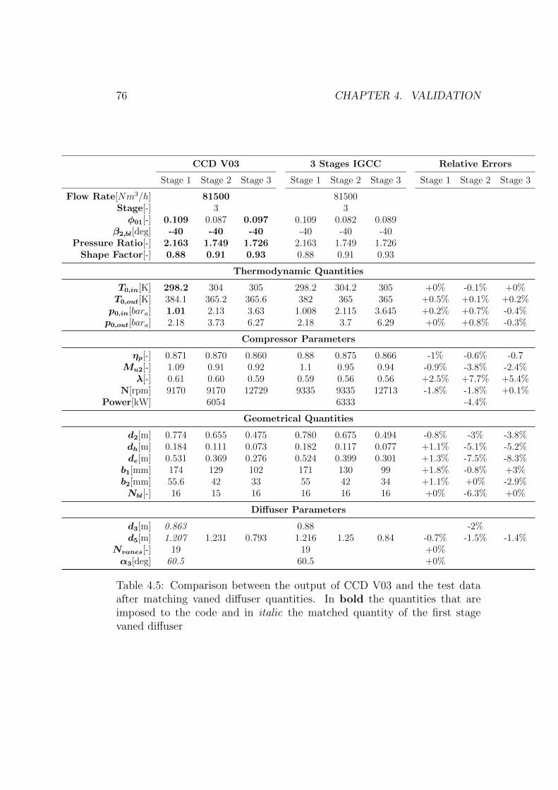
76 CHAPTER 4. VALIDATION
CCD V03 3 Stages IGCC Relative Errors
Stage 1 Stage 2 Stage 3 Stage 1 Stage 2 Stage 3 Stage 1 Stage 2 Stage 3
Flow Rate[Nm3/h] 81500 81500Stage[-] 3 3φ01[-] 0.109 0.087 0.097 0.109 0.082 0.089
β2,bl[deg] -40 -40 -40 -40 -40 -40Pressure Ratio[-] 2.163 1.749 1.726 2.163 1.749 1.726
Shape Factor[-] 0.88 0.91 0.93 0.88 0.91 0.93
Thermodynamic Quantities
T0,in[K] 298.2 304 305 298.2 304.2 305 +0% -0.1% +0%T0,out[K] 384.1 365.2 365.6 382 365 365 +0.5% +0.1% +0.2%p0,in[bara] 1.01 2.13 3.63 1.008 2.115 3.645 +0.2% +0.7% -0.4%p0,out[bara] 2.18 3.73 6.27 2.18 3.7 6.29 +0% +0.8% -0.3%
Compressor Parameters
ηp[-] 0.871 0.870 0.860 0.88 0.875 0.866 -1% -0.6% -0.7Mu2[-] 1.09 0.91 0.92 1.1 0.95 0.94 -0.9% -3.8% -2.4%λ[-] 0.61 0.60 0.59 0.59 0.56 0.56 +2.5% +7.7% +5.4%
N[rpm] 9170 9170 12729 9335 9335 12713 -1.8% -1.8% +0.1%Power[kW] 6054 6333 -4.4%
Geometrical Quantities
d2[m] 0.774 0.655 0.475 0.780 0.675 0.494 -0.8% -3% -3.8%dh[m] 0.184 0.111 0.073 0.182 0.117 0.077 +1.1% -5.1% -5.2%de[m] 0.531 0.369 0.276 0.524 0.399 0.301 +1.3% -7.5% -8.3%b1[mm] 174 129 102 171 130 99 +1.8% -0.8% +3%b2[mm] 55.6 42 33 55 42 34 +1.1% +0% -2.9%Nbl[-] 16 15 16 16 16 16 +0% -6.3% +0%
Diffuser Parameters
d3[m] 0.863 0.88 -2%d5[m] 1.207 1.231 0.793 1.216 1.25 0.84 -0.7% -1.5% -1.4%
Nvanes[-] 19 19 +0%α3[deg] 60.5 60.5 +0%
Table 4.5: Comparison between the output of CCD V03 and the test dataafter matching vaned diffuser quantities. In bold the quantities that areimposed to the code and in italic the matched quantity of the first stagevaned diffuser
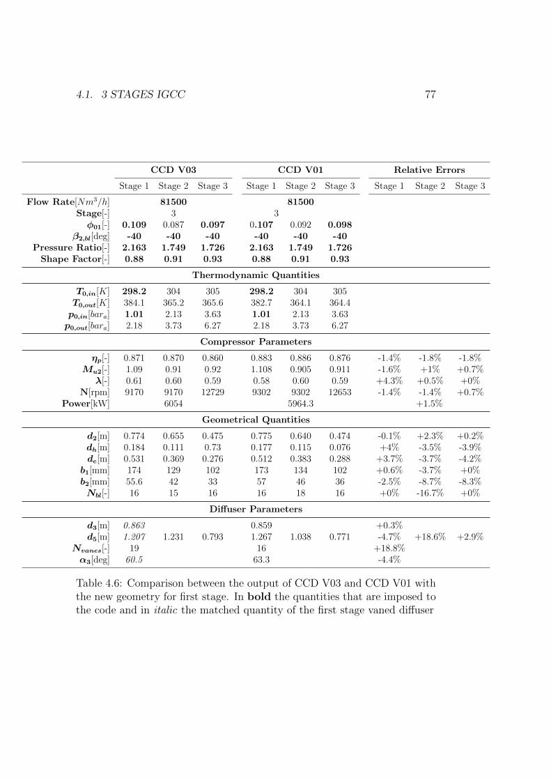
4.1. 3 STAGES IGCC 77
CCD V03 CCD V01 Relative Errors
Stage 1 Stage 2 Stage 3 Stage 1 Stage 2 Stage 3 Stage 1 Stage 2 Stage 3
Flow Rate[Nm3/h] 81500 81500Stage[-] 3 3φ01[-] 0.109 0.087 0.097 0.107 0.092 0.098
β2,bl[deg] -40 -40 -40 -40 -40 -40Pressure Ratio[-] 2.163 1.749 1.726 2.163 1.749 1.726
Shape Factor[-] 0.88 0.91 0.93 0.88 0.91 0.93
Thermodynamic Quantities
T0,in[K] 298.2 304 305 298.2 304 305T0,out[K] 384.1 365.2 365.6 382.7 364.1 364.4p0,in[bara] 1.01 2.13 3.63 1.01 2.13 3.63p0,out[bara] 2.18 3.73 6.27 2.18 3.73 6.27
Compressor Parameters
ηp[-] 0.871 0.870 0.860 0.883 0.886 0.876 -1.4% -1.8% -1.8%Mu2[-] 1.09 0.91 0.92 1.108 0.905 0.911 -1.6% +1% +0.7%λ[-] 0.61 0.60 0.59 0.58 0.60 0.59 +4.3% +0.5% +0%
N[rpm] 9170 9170 12729 9302 9302 12653 -1.4% -1.4% +0.7%Power[kW] 6054 5964.3 +1.5%
Geometrical Quantities
d2[m] 0.774 0.655 0.475 0.775 0.640 0.474 -0.1% +2.3% +0.2%dh[m] 0.184 0.111 0.73 0.177 0.115 0.076 +4% -3.5% -3.9%de[m] 0.531 0.369 0.276 0.512 0.383 0.288 +3.7% -3.7% -4.2%b1[mm] 174 129 102 173 134 102 +0.6% -3.7% +0%b2[mm] 55.6 42 33 57 46 36 -2.5% -8.7% -8.3%Nbl[-] 16 15 16 16 18 16 +0% -16.7% +0%
Diffuser Parameters
d3[m] 0.863 0.859 +0.3%d5[m] 1.207 1.231 0.793 1.267 1.038 0.771 -4.7% +18.6% +2.9%
Nvanes[-] 19 16 +18.8%α3[deg] 60.5 63.3 -4.4%
Table 4.6: Comparison between the output of CCD V03 and CCD V01 withthe new geometry for first stage. In bold the quantities that are imposed tothe code and in italic the matched quantity of the first stage vaned diffuser
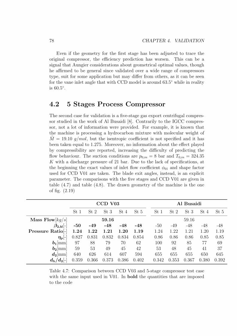
78 CHAPTER 4. VALIDATION
Even if the geometry for the first stage has been adjusted to trace theoriginal compressor, the efficiency prediction has worsen. This can be asignal that Aungier considerations about geometrical optimal values, thoughhe affirmed to be general since validated over a wide range of compressorstype, suit for some application but may differ from others, as it can be seenfor the vane inlet angle that with CCD model is around 63.5◦ while in realityis 60.5◦.
4.2 5 Stages Process Compressor
The second case for validation is a five-stage gas export centrifugal compres-sor studied in the work of Al Busaidi [8]. Contrarily to the IGCC compres-sor, not a lot of information were provided. For example, it is known thatthe machine is processing a hydrocarbon mixture with molecular weight ofM = 19.10 g/mol, but the isentropic coefficient is not specified and it hasbeen taken equal to 1.275. Moreover, no information about the effect playedby compressibility are reported, increasing the difficulty of predicting theflow behaviour. The suction conditions are p0,in = 8 bar and T0,in = 324.35K with a discharge pressure of 21 bar. Due to the lack of specifications, atthe beginning the exact values of inlet flow coefficient φ01 and shape factorused for CCD V01 are taken. The blade exit angles, instead, is an explicitparameter. The comparisons with the five stages and CCD V01 are given intable (4.7) and table (4.8). The drawn geometry of the machine is the oneof fig. (2.19)
CCD V03 Al Busaidi
St 1 St 2 St 3 St 4 St 5 St 1 St 2 St 3 St 4 St 5
Mass Flow[kg/s] 59.16 59.16β2,bl[-] -50 -49 -48 -48 -48 -50 -49 -48 -48 -48
Pressure Ratio[-] 1.24 1.22 1.21 1.20 1.19 1.24 1.22 1.21 1.20 1.19ηp[-] 0.827 0.831 0.832 0.834 0.854 0.86 0.86 0.86 0.85 0.85
b1[mm] 97 88 79 70 62 100 92 85 77 69b2[mm] 59 53 49 45 42 53 48 45 41 37d2[mm] 640 626 614 607 594 655 655 655 650 645dh/d2[-] 0.359 0.366 0.373 0.386 0.402 0.342 0.353 0.367 0.380 0.392
Table 4.7: Comparison between CCD V03 and 5-stage compressor test casewith the same input used in V01. In bold the quantities that are imposedto the code
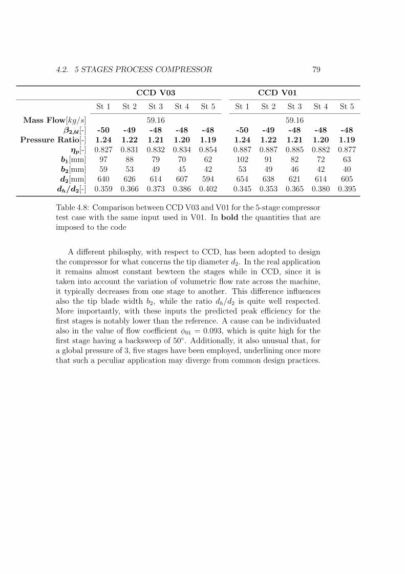
4.2. 5 STAGES PROCESS COMPRESSOR 79
CCD V03 CCD V01
St 1 St 2 St 3 St 4 St 5 St 1 St 2 St 3 St 4 St 5
Mass Flow[kg/s] 59.16 59.16β2,bl[-] -50 -49 -48 -48 -48 -50 -49 -48 -48 -48
Pressure Ratio[-] 1.24 1.22 1.21 1.20 1.19 1.24 1.22 1.21 1.20 1.19ηp[-] 0.827 0.831 0.832 0.834 0.854 0.887 0.887 0.885 0.882 0.877
b1[mm] 97 88 79 70 62 102 91 82 72 63b2[mm] 59 53 49 45 42 53 49 46 42 40d2[mm] 640 626 614 607 594 654 638 621 614 605dh/d2[-] 0.359 0.366 0.373 0.386 0.402 0.345 0.353 0.365 0.380 0.395
Table 4.8: Comparison between CCD V03 and V01 for the 5-stage compressortest case with the same input used in V01. In bold the quantities that areimposed to the code
A different philosphy, with respect to CCD, has been adopted to designthe compressor for what concerns the tip diameter d2. In the real applicationit remains almost constant bewteen the stages while in CCD, since it istaken into account the variation of volumetric flow rate across the machine,it typically decreases from one stage to another. This difference influencesalso the tip blade width b2, while the ratio dh/d2 is quite well respected.More importantly, with these inputs the predicted peak efficiency for thefirst stages is notably lower than the reference. A cause can be individuatedalso in the value of flow coefficient φ01 = 0.093, which is quite high for thefirst stage having a backsweep of 50◦. Additionally, it also unusual that, fora global pressure of 3, five stages have been employed, underlining once morethat such a peculiar application may diverge from common design practices.

80 CHAPTER 4. VALIDATION
4.2.1 Off-design 5 stages
The interesting aspect of this validation case is the range on which compressormaps data have been provided, with speedlines from 60% to 100%. In thisway, it is possible to compare how Casey and Robinson model will behavefar from the operational speedline. Since the compressor to deal with is ofprocess type, similar parameters to the previous case are employed here (seetable (4.9) and table (4.10)), with the exception of B that is set to 0.55according to the mean Mach number of the machine, which is indeed around0.55, in order to give the blending function P an almost identical parametervariation trend among the stages.
A B C As Bs Cs
1 0.55 5 0 0.55 4.75
Table 4.9: 5 stages off design paramters for blending function
D G H φP/φC φS/φC
Low Mach 1.7 2 2 0.50 0.225High Mach 2.1 0.3 3.5 0.95 0.835
Table 4.10: 5 stages off design parameters
The pressure ratio is well estimated for what concerns the lower speedlinesbut loses effectiveness close to surge line when the speed increases. Surely,the fact that design point is not on the 100% speedline but just a bit lowerhas an impact on the shift (if the highest speedline is corrected a more similartrend is shown, as depicted in fig. (4.7)).
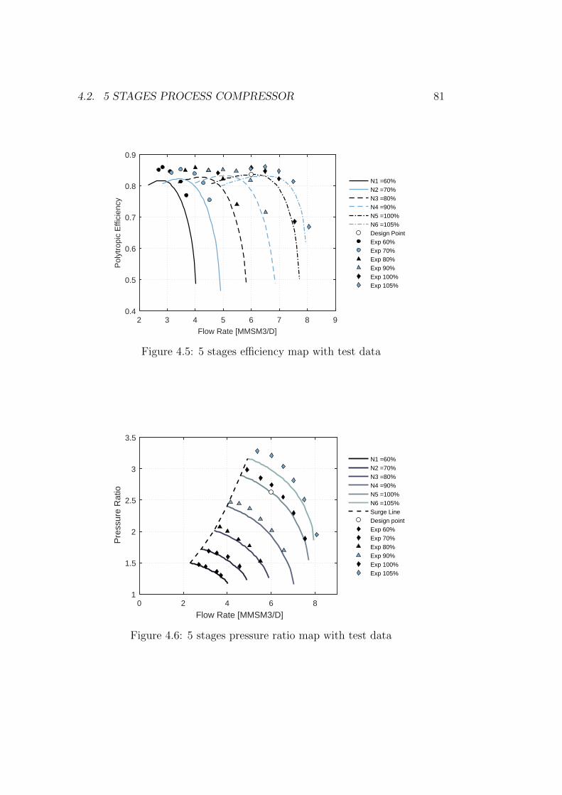
4.2. 5 STAGES PROCESS COMPRESSOR 81
2 3 4 5 6 7 8 9Flow Rate [MMSM3/D]
0.4
0.5
0.6
0.7
0.8
0.9
Pol
ytro
pic
Effi
cien
cy
N1 =60%N2 =70%N3 =80%N4 =90%N5 =100%N6 =105%Design PointExp 60%Exp 70%Exp 80%Exp 90%Exp 100%Exp 105%
Figure 4.5: 5 stages efficiency map with test data
0 2 4 6 8
Flow Rate [MMSM3/D]
1
1.5
2
2.5
3
3.5
Pre
ssur
e R
atio
N1 =60%N2 =70%N3 =80%N4 =90%N5 =100%N6 =105%Surge LineDesign pointExp 60%Exp 70%Exp 80%Exp 90%Exp 100%Exp 105%
Figure 4.6: 5 stages pressure ratio map with test data
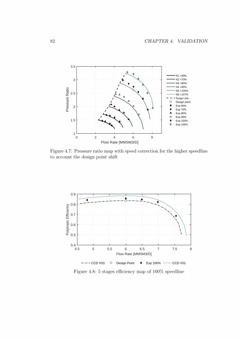
82 CHAPTER 4. VALIDATION
0 2 4 6 8
Flow Rate [MMSM3/D]
1
1.5
2
2.5
3
3.5P
ress
ure
Rat
io
N1 =60%N2 =70%N3 =80%N4 =90%N5 =100%N6 =107%Surge LineDesign pointExp 60%Exp 70%Exp 80%Exp 90%Exp 100%Exp 105%
Figure 4.7: Pressure ratio map with speed correction for the higher speedlineto account the design point shift
4.5 5 5.5 6 6.5 7 7.5 8Flow Rate [MMSM3/D]
0.4
0.5
0.6
0.7
0.8
0.9
Pol
ytro
pic
Effi
cien
cy
CCD V03 Design Point Exp 100% CCD V01
Figure 4.8: 5 stages efficiency map of 100% speedline
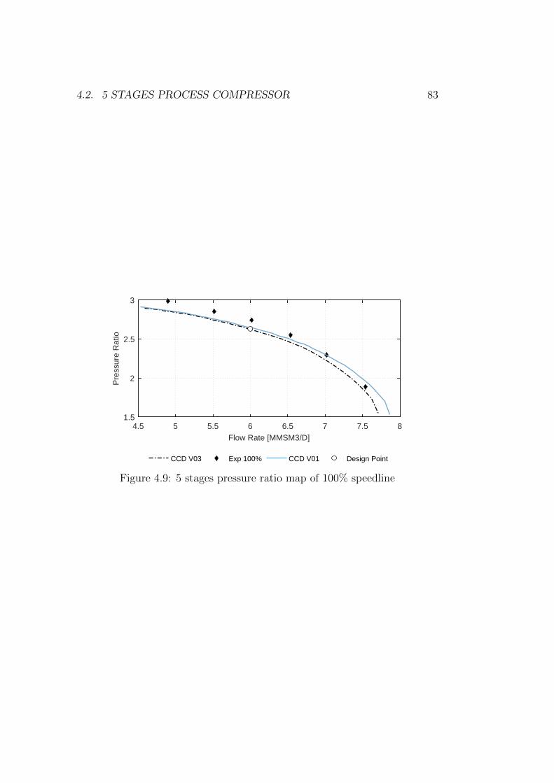
4.2. 5 STAGES PROCESS COMPRESSOR 83
4.5 5 5.5 6 6.5 7 7.5 8Flow Rate [MMSM3/D]
1.5
2
2.5
3
Pre
ssur
e R
atio
CCD V03 Exp 100% CCD V01 Design Point
Figure 4.9: 5 stages pressure ratio map of 100% speedline
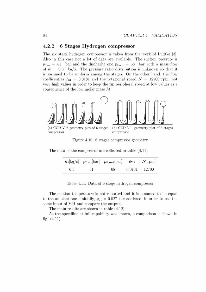
84 CHAPTER 4. VALIDATION
4.2.2 6 Stages Hydrogen compressor
The six stage hydrogen compressor is taken from the work of Ludtke [3].Also in this case not a lot of data are available. The suction pressure isp0,in = 51 bar and the discharhe one p0,out = 58 bar with a mass flowof m = 6.3 kg/s. The pressure ratio distribution is unknown so that itis assumed to be uniform among the stages. On the other hand, the flowcoefficent is φ01 = 0.0181 and the rotational speed N = 12700 rpm, notvery high values in order to keep the tip peripheral speed at low values as aconsequence of the low molar mass M .
(a) CCD V03 geometry plot of 6 stagescompressor
(b) CCD V01 geometry plot of 6 stagescompressor
Figure 4.10: 6 stages compressor geometry
The data of the compressor are collected in table (4.11)
m[kg/s] p0.in[bar] p0,out[bar] φ01 N [rpm]
6.3 51 68 0.0181 12700
Table 4.11: Data of 6 stage hydrogen compressor
The suction temperature is not reported and it is assumed to be equalto the ambient one. Initially, φ01 = 0.027 is considered, in order to use thesame input of V01 and compare the outputs.
The main results are shown in table (4.12)As the speedline at full capability was known, a comparison is shown in
fig. (4.11).
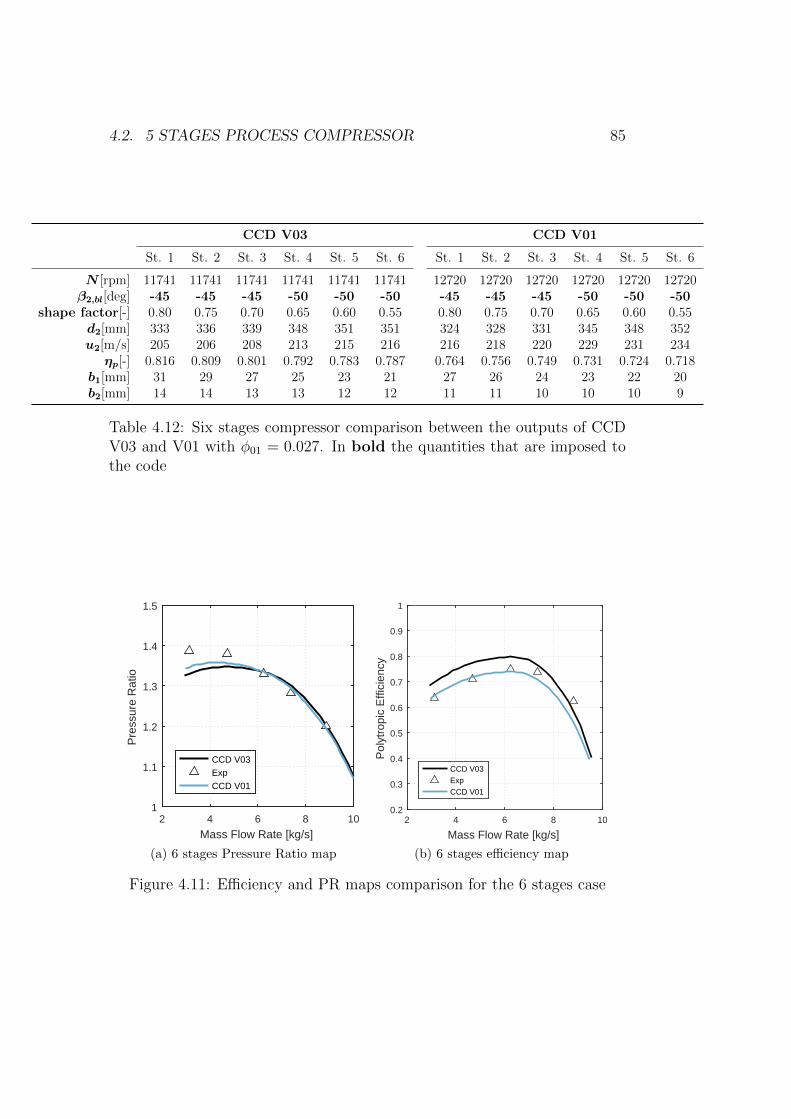
4.2. 5 STAGES PROCESS COMPRESSOR 85
CCD V03 CCD V01
St. 1 St. 2 St. 3 St. 4 St. 5 St. 6 St. 1 St. 2 St. 3 St. 4 St. 5 St. 6
N [rpm] 11741 11741 11741 11741 11741 11741 12720 12720 12720 12720 12720 12720β2,bl[deg] -45 -45 -45 -50 -50 -50 -45 -45 -45 -50 -50 -50
shape factor[-] 0.80 0.75 0.70 0.65 0.60 0.55 0.80 0.75 0.70 0.65 0.60 0.55d2[mm] 333 336 339 348 351 351 324 328 331 345 348 352u2[m/s] 205 206 208 213 215 216 216 218 220 229 231 234ηp[-] 0.816 0.809 0.801 0.792 0.783 0.787 0.764 0.756 0.749 0.731 0.724 0.718
b1[mm] 31 29 27 25 23 21 27 26 24 23 22 20b2[mm] 14 14 13 13 12 12 11 11 10 10 10 9
Table 4.12: Six stages compressor comparison between the outputs of CCDV03 and V01 with φ01 = 0.027. In bold the quantities that are imposed tothe code
2 4 6 8 10
Mass Flow Rate [kg/s]
1
1.1
1.2
1.3
1.4
1.5
Pre
ssur
e R
atio
CCD V03ExpCCD V01
(a) 6 stages Pressure Ratio map
2 4 6 8 10
Mass Flow Rate [kg/s]
0.2
0.3
0.4
0.5
0.6
0.7
0.8
0.9
1
Pol
ytro
pic
Effi
cien
cy
CCD V03ExpCCD V01
(b) 6 stages efficiency map
Figure 4.11: Efficiency and PR maps comparison for the 6 stages case
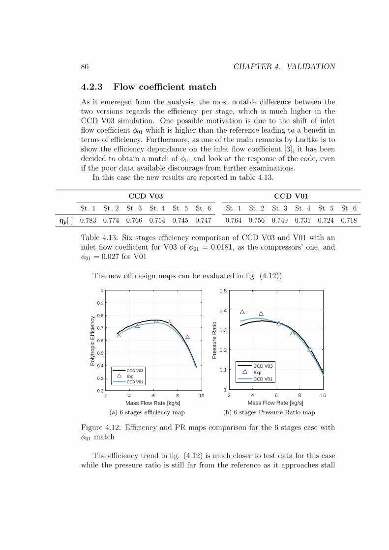
86 CHAPTER 4. VALIDATION
4.2.3 Flow coefficient match
As it emereged from the analysis, the most notable difference between thetwo versions regards the efficiency per stage, which is much higher in theCCD V03 simulation. One possible motivation is due to the shift of inletflow coefficient φ01 which is higher than the reference leading to a benefit interms of efficiency. Furthermore, as one of the main remarks by Ludtke is toshow the efficiency dependance on the inlet flow coefficient [3], it has beendecided to obtain a match of φ01 and look at the response of the code, evenif the poor data available discourage from further examinations.
In this case the new results are reported in table 4.13.
CCD V03 CCD V01
St. 1 St. 2 St. 3 St. 4 St. 5 St. 6 St. 1 St. 2 St. 3 St. 4 St. 5 St. 6
ηp[-] 0.783 0.774 0.766 0.754 0.745 0.747 0.764 0.756 0.749 0.731 0.724 0.718
Table 4.13: Six stages efficiency comparison of CCD V03 and V01 with aninlet flow coefficient for V03 of φ01 = 0.0181, as the compressors’ one, andφ01 = 0.027 for V01
The new off design maps can be evaluated in fig. (4.12))
2 4 6 8 10
Mass Flow Rate [kg/s]
0.2
0.3
0.4
0.5
0.6
0.7
0.8
0.9
1
Pol
ytro
pic
Effi
cien
cy
CCD V03ExpCCD V01
(a) 6 stages efficiency map
2 4 6 8 10
Mass Flow Rate [kg/s]
1
1.1
1.2
1.3
1.4
1.5
Pre
ssur
e R
atio
CCD V03ExpCCD V01
(b) 6 stages Pressure Ratio map
Figure 4.12: Efficiency and PR maps comparison for the 6 stages case withφ01 match
The efficiency trend in fig. (4.12) is much closer to test data for this casewhile the pressure ratio is still far from the reference as it approaches stall
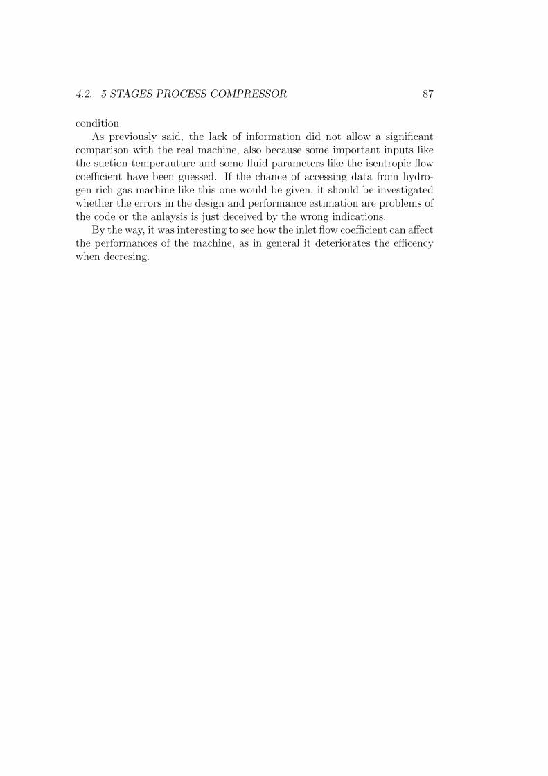
4.2. 5 STAGES PROCESS COMPRESSOR 87
condition.As previously said, the lack of information did not allow a significant
comparison with the real machine, also because some important inputs likethe suction temperauture and some fluid parameters like the isentropic flowcoefficient have been guessed. If the chance of accessing data from hydro-gen rich gas machine like this one would be given, it should be investigatedwhether the errors in the design and performance estimation are problems ofthe code or the anlaysis is just deceived by the wrong indications.
By the way, it was interesting to see how the inlet flow coefficient can affectthe performances of the machine, as in general it deteriorates the efficencywhen decresing.
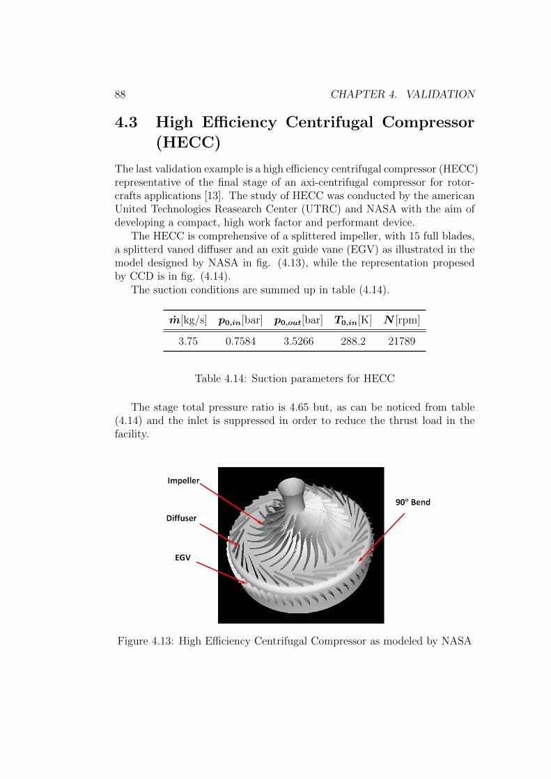
88 CHAPTER 4. VALIDATION
4.3 High Efficiency Centrifugal Compressor
(HECC)
The last validation example is a high efficiency centrifugal compressor (HECC)representative of the final stage of an axi-centrifugal compressor for rotor-crafts applications [13]. The study of HECC was conducted by the americanUnited Technologies Reasearch Center (UTRC) and NASA with the aim ofdeveloping a compact, high work factor and performant device.
The HECC is comprehensive of a splittered impeller, with 15 full blades,a splitterd vaned diffuser and an exit guide vane (EGV) as illustrated in themodel designed by NASA in fig. (4.13), while the representation propesedby CCD is in fig. (4.14).
The suction conditions are summed up in table (4.14).
m[kg/s] p0,in[bar] p0,out[bar] T0,in[K] N [rpm]
3.75 0.7584 3.5266 288.2 21789
Table 4.14: Suction parameters for HECC
The stage total pressure ratio is 4.65 but, as can be noticed from table(4.14) and the inlet is suppressed in order to reduce the thrust load in thefacility.
Figure 4.13: High Efficiency Centrifugal Compressor as modeled by NASA
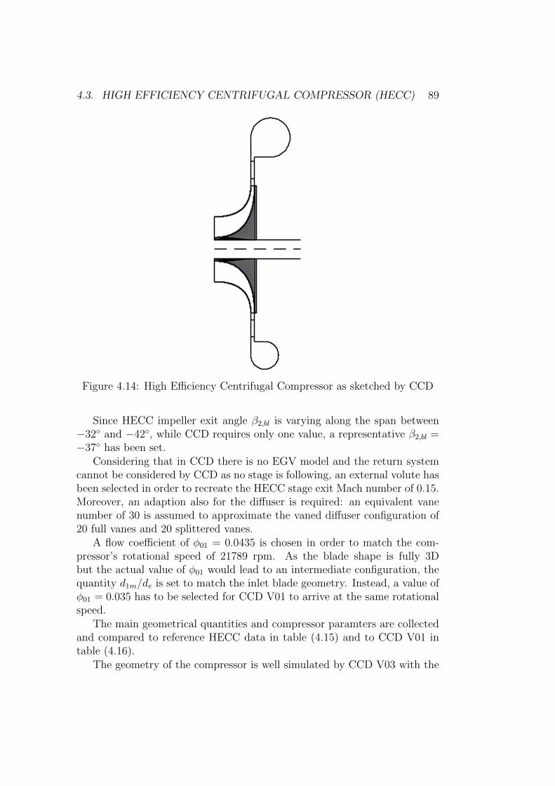
4.3. HIGH EFFICIENCY CENTRIFUGAL COMPRESSOR (HECC) 89
Figure 4.14: High Efficiency Centrifugal Compressor as sketched by CCD
Since HECC impeller exit angle β2,bl is varying along the span between−32◦ and −42◦, while CCD requires only one value, a representative β2,bl =−37◦ has been set.
Considering that in CCD there is no EGV model and the return systemcannot be considered by CCD as no stage is following, an external volute hasbeen selected in order to recreate the HECC stage exit Mach number of 0.15.Moreover, an adaption also for the diffuser is required: an equivalent vanenumber of 30 is assumed to approximate the vaned diffuser configuration of20 full vanes and 20 splittered vanes.
A flow coefficient of φ01 = 0.0435 is chosen in order to match the com-pressor’s rotational speed of 21789 rpm. As the blade shape is fully 3Dbut the actual value of φ01 would lead to an intermediate configuration, thequantity d1m/de is set to match the inlet blade geometry. Instead, a value ofφ01 = 0.035 has to be selected for CCD V01 to arrive at the same rotationalspeed.
The main geometrical quantities and compressor paramters are collectedand compared to reference HECC data in table (4.15) and to CCD V01 intable (4.16).
The geometry of the compressor is well simulated by CCD V03 with the
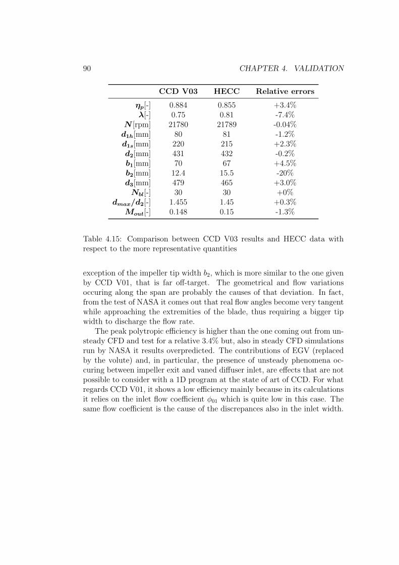
90 CHAPTER 4. VALIDATION
CCD V03 HECC Relative errors
ηp[-] 0.884 0.855 +3.4%λ[-] 0.75 0.81 -7.4%
N [rpm] 21780 21789 -0.04%d1h[mm] 80 81 -1.2%d1s[mm] 220 215 +2.3%d2[mm] 431 432 -0.2%b1[mm] 70 67 +4.5%b2[mm] 12.4 15.5 -20%d3[mm] 479 465 +3.0%Nbl[-] 30 30 +0%
dmax/d2[-] 1.455 1.45 +0.3%Mout[-] 0.148 0.15 -1.3%
Table 4.15: Comparison between CCD V03 results and HECC data withrespect to the more representative quantities
exception of the impeller tip width b2, which is more similar to the one givenby CCD V01, that is far off-target. The geometrical and flow variationsoccuring along the span are probably the causes of that deviation. In fact,from the test of NASA it comes out that real flow angles become very tangentwhile approaching the extremities of the blade, thus requiring a bigger tipwidth to discharge the flow rate.
The peak polytropic efficiency is higher than the one coming out from un-steady CFD and test for a relative 3.4% but, also in steady CFD simulationsrun by NASA it results overpredicted. The contributions of EGV (replacedby the volute) and, in particular, the presence of unsteady phenomena oc-curing between impeller exit and vaned diffuser inlet, are effects that are notpossible to consider with a 1D program at the state of art of CCD. For whatregards CCD V01, it shows a low efficiency mainly because in its calculationsit relies on the inlet flow coefficient φ01 which is quite low in this case. Thesame flow coefficient is the cause of the discrepances also in the inlet width.
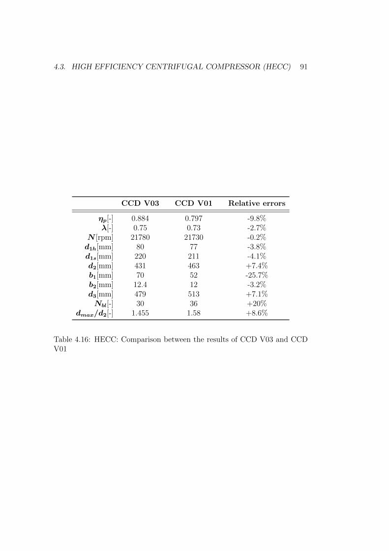
4.3. HIGH EFFICIENCY CENTRIFUGAL COMPRESSOR (HECC) 91
CCD V03 CCD V01 Relative errors
ηp[-] 0.884 0.797 -9.8%λ[-] 0.75 0.73 -2.7%
N [rpm] 21780 21730 -0.2%d1h[mm] 80 77 -3.8%d1s[mm] 220 211 -4.1%d2[mm] 431 463 +7.4%b1[mm] 70 52 -25.7%b2[mm] 12.4 12 -3.2%d3[mm] 479 513 +7.1%Nbl[-] 30 36 +20%
dmax/d2[-] 1.455 1.58 +8.6%
Table 4.16: HECC: Comparison between the results of CCD V03 and CCDV01
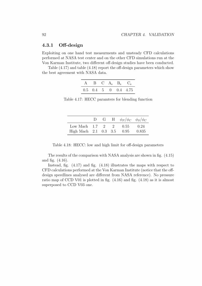
92 CHAPTER 4. VALIDATION
4.3.1 Off-design
Exploiting on one hand test measurments and unsteady CFD calculationsperformed at NASA test center and on the other CFD simulations run at theVon Karman Institute, two different off-design studies have been conducted.
Table (4.17) and table (4.18) report the off-design parameters which showthe best agreement with NASA data.
A B C As Bs Cs
0.5 0.4 5 0 0.4 4.75
Table 4.17: HECC paramters for blending function
D G H φP/φC φS/φC
Low Mach 1.7 2 2 0.55 0.24High Mach 2.1 0.3 3.5 0.95 0.835
Table 4.18: HECC: low and high limit for off-design parameters
The results of the comparison with NASA analysis are shown in fig. (4.15)and fig. (4.16).
Instead, fig. (4.17) and fig. (4.18) illustrates the maps with respect toCFD calculations performed at the Von Karman Institute (notice that the off-design speedlines analysed are different from NASA reference). No pressureratio map of CCD V01 is plotted in fig. (4.16) and fig. (4.18) as it is almostsuperposed to CCD V03 one.
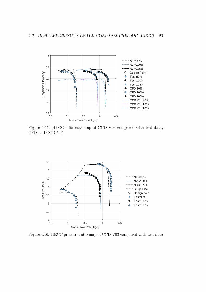
4.3. HIGH EFFICIENCY CENTRIFUGAL COMPRESSOR (HECC) 93
2.5 3 3.5 4 4.5
Mass Flow Rate [kg/s]
0.5
0.6
0.7
0.8
0.9
1
Pol
ytro
pic
Effi
cien
cy
N1 =90%N2 =100%N3 =105%Design PointTest 90%Test 100%Test 105%CFD 90%CFD 100%CFD 105%CCD V01 90%CCD V01 100%CCD V01 105%
Figure 4.15: HECC efficiency map of CCD V03 compared with test data,CFD and CCD V01
2.5 3 3.5 4 4.5
Mass Flow Rate [kg/s]
2
2.5
3
3.5
4
4.5
5
5.5
Pre
ssur
e R
atio
N1 =90%N2 =100%N3 =105%Surge LineDesign pointTest 90%Test 100%Test 105%
Figure 4.16: HECC pressure ratio map of CCD V03 compared with test data
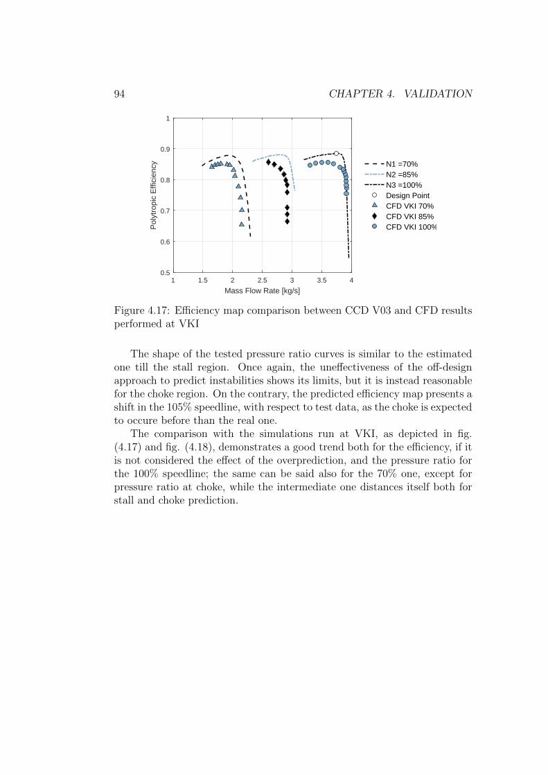
94 CHAPTER 4. VALIDATION
1 1.5 2 2.5 3 3.5 4
Mass Flow Rate [kg/s]
0.5
0.6
0.7
0.8
0.9
1
Pol
ytro
pic
Effi
cien
cy N1 =70%N2 =85%N3 =100%Design PointCFD VKI 70%CFD VKI 85%CFD VKI 100%
Figure 4.17: Efficiency map comparison between CCD V03 and CFD resultsperformed at VKI
The shape of the tested pressure ratio curves is similar to the estimatedone till the stall region. Once again, the uneffectiveness of the off-designapproach to predict instabilities shows its limits, but it is instead reasonablefor the choke region. On the contrary, the predicted efficiency map presents ashift in the 105% speedline, with respect to test data, as the choke is expectedto occure before than the real one.
The comparison with the simulations run at VKI, as depicted in fig.(4.17) and fig. (4.18), demonstrates a good trend both for the efficiency, if itis not considered the effect of the overprediction, and the pressure ratio forthe 100% speedline; the same can be said also for the 70% one, except forpressure ratio at choke, while the intermediate one distances itself both forstall and choke prediction.
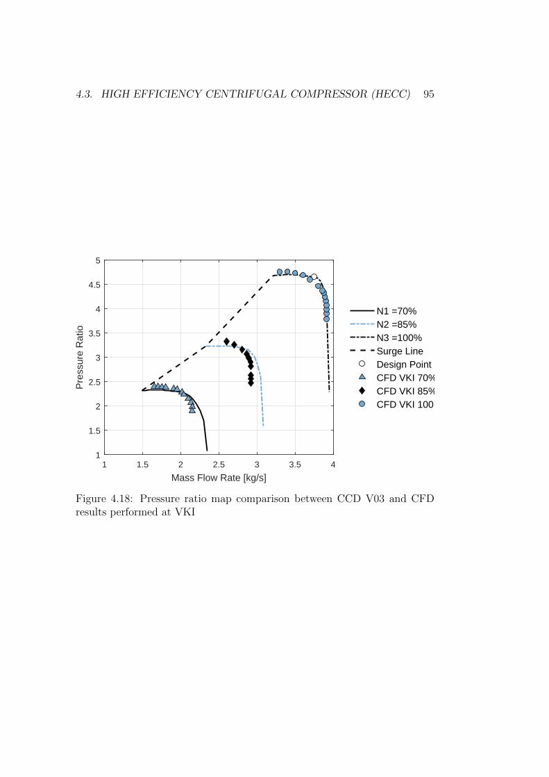
4.3. HIGH EFFICIENCY CENTRIFUGAL COMPRESSOR (HECC) 95
1 1.5 2 2.5 3 3.5 4
Mass Flow Rate [kg/s]
1
1.5
2
2.5
3
3.5
4
4.5
5
Pre
ssur
e R
atio
N1 =70%N2 =85%N3 =100%Surge LineDesign PointCFD VKI 70%CFD VKI 85%CFD VKI 100
Figure 4.18: Pressure ratio map comparison between CCD V03 and CFDresults performed at VKI
96 CHAPTER 4. VALIDATION
4.4 Summary of Validation Tests
Four reference cases have been considered to validate the capability of thenew program, through an implemented loss model for the main components,to provide a reliable design and well predict the peak performances of acentrifugal compressor. For the first case in particular, both the geometricaland thermodynamic quantities confirm a good agreement with the referencedata and also the efficiency is within a reasonable margin of error for all thestages, as it was for CCD V01.
Since the approach for the off-design is conducted in a very similar way, nosurprise is encountered in discovering that the behaviour of the two versionsis almost identical, when they have comparable starting points. Moreover,even if only few input parameters are requested by CCD to run an analysis,the first test shows the importance of having all the pivotal data available,in order to leave to chance the less possible guesses. In fact, as case twoand three pointed out, the comparison is made more difficult when severalunknown paramters can deceive it. In general, it seems that one characteristicof the loss model has been to attenuate the strong influence of the inlet flowcoefficient in the determination of the efficiency, evaluating it on physicalbased correlations. As a matter of fact, even if it is of course generallytrue the dependence on φ01, in some cases you can get good performancesalso for not high values of φ01, as realised from the turbocharger compressorsimulation.
Finally, it has to be clarified that the loss model has been validated asa whole, meaning that the performance of the entire machine have beencompared with baseline references, since it was not possible to perform acomponent by component off-design analysis as it is not implemented in thecode.
Chapter 5
Conclusions
A new one-dimensional methodology for the design and performance predic-tion of multi-stage centrifugal compressors has been programmed in a newversion of MatlabR© program CCD, obtaining encouraging feedbacks fromtestings. The current tool can be a helpful support for the designer whenreceiving a commission from a costumer. In fact, using the few specifica-tions that would be given, among which mass flow, fluid suction conditionsand total pressure ratio, CCD addresses the designer towards a reasonableconfiguration of the most important components of a centrifugal compressorlike the impeller, the vaneless and vaned diffuser, the return system and thevolute. New design methodologies based on good design practices have beenindeed incorporated in CCD in order to size them. To give more flexibility tothe user, in an input file the possibility of assembling an arbitrary compressorhas been given by specifying the desired components that will compose themachine, plus controlling some settings about their principal characteristics.
Since one of the biggest issues when dealing with a turbomachine is thecomputation of the losses occuring in it, a comprehensive 1D loss modelprovided by Aungier [1] has been implemented in the code for all the elementsof the compressor, allowing to properly evaluate the performances at designpoint through the use of correlations that rely on the geometrical and flowquantities previously calculated. For what concernss the off-design, instead,an approach based on non-dimensional parameters has been followed. Infact, even if the the loss correlations employed can be applied for off-designconditions, it was not possile to simply change the inlet mass flow in the inputfile to obtain the performance and efficiency maps because this would havelead to a variation of the geometry of the compressor, as the main routine issuited for a design process. Therefore, a specific procedure has to be studiedto perform such calculations and it can be a topic for a future work on CCD.
97
98 CHAPTER 5. CONCLUSIONS
5.1 Future Works
Multi-objectve optimization
In the estimation of the performaces of a compressor the efficiency is notthe only parameter to worry about but also a wide range of operationhas to be accounted. Since CCD predicts only one reasonable designbut maybe not the best one, it can be useful to run an optimizationwhich guides the designer towards the most appropriate configurationfor the required compressor. Currently, some optimization analyses arealready running at the Von Karman Institute in order to be able toachieve this goal.
New programming language When a multi-objective optimization isconsidered important, the need of quick simulations becomes reallypivotal as thousands of them have to be carried out. Since the couplingof an optimization sofwtare with Matlab is not efficient, a transaltionof CCD to Python may be the right choice to pick, so that even anarticulate optimization can be done in a reasonable time.
Off-design
The next step for CCD is the use the loss correlation models also forthe off-design, comparing the results with respect to Casey and Robin-son approach. This will be possible by implementing another seprateroutine which takes in input the main geometrical quantities obtainedduring the design phase. For each speedline, choke condition can beevaluated from the velocity which causes choke in the throat whilestall condition can be decided by fixing a limit value for diffusion ra-tio w1s/w2. The thermodynamic quantities are calculated in order toestimate the efficiency and the pressure ratio.
Modeling of new components Some missing components that could beadditionally modeled in CCD are represented by regulation systemssuch as Inlet Guide Vane (IGV) or diffuser guide vane (DGV). Withthis addition, also a more proper off-design analysis could be carriedout.
Real gas behaviour Even if the compressibility effect in a compressor isnot as much important as in a gas turbine, where the temperatures canbe incredibly high, the use of more powerful thermodynamic correlationcan be employed to better estimate the properties of the fluid acrossthe machine, so to render the 1D performance analysis more reliable.
Chapter 6
References
[1] R.H. Aungier, Centrifugal Compressors: a Strategy for Aerodynamic De-sign and Analysis, ASME PRESS 2000
[2] M. Casey, C. Robinson A method to estimate the Performnce Map ofa Centrifugal Compressor Stage, Journal of Turbomachinery, November 2012
[3] K.H. Ludtke, Process Centrifugal Compressor: Basics, Function, Op-eration, Design, Application , Springer 2004
[4] P. Harley, S. Spence, D. Filsinger, M. Dietrich and J. Early Assessing1D Loss Models for the Off-Design Performance Prediction of AutomotiveTurbocharger Compressors June 2013
[5] A. Whitfield, N. C. Baines Design of Radial Turbomachines, LongmanSingapor Publisher (Pte) Ltd., 1990
[6] N. Cumpsty, Compressor Aerodynamics, Krieger Publishing Company,1989
[7] M. Casey and M. Schlegel, Estimation of the performance of turbochargercompressors at extremely low pressure ratios, Proceedings of the Institutionof Mechanical Engineers, Part A: Journal of Power and Energy, vol. 224, no.2, pp. 239-250, 2010
[8] W. Al-Busaidi and P. Pilidis, A new method for reliable performance pre-diction of multi-stage industrial centrifugal compresors based on stage stack-ing technique: Part I - existing models evaluation, Applied Thermal Engi-neering, vol. 98, pp. 10 - 28, 2016
99
100 CHAPTER 6. REFERENCES
[9] A. Srinivasan and C. Impastato, Application of integral geared compres-sors in the process gas industry, ASME, vol. GT, no. 95870, 2013
[10] P. Dalbert, M. Casey, and E.Schurter, Development testing and per-formance prediction of radial compressor stages for multi-stage industrialcompressors, Thermal Engineering, vol. 88-GT-34, 1988
[11] R. Van den Braembussche, Centrifugal Compressors: Analysis and De-sign. Course Note 192, 2015
[12] A. Romei, Design and optimization of multi-stage centrifugal compres-sors with uncertainty quantification of off design performances, Master The-sis, Polytechnic of Milan, 2016
[13] G. Medic et al., High efficiency centrifugal compressors for rotorcraftapplications, NASA/CR-2014-218114
[14] R. H. Aungier, Centrifugal compressor stage preliminary aerodynamicdesign and component sizing, ASME 95-GT-78
[15] R. H. Aungier, Aerodynamic design and analysis of vaneless diffusersand return channels, ASME 93-GT-101, 1993
[16] R. H. Aungier, Mean streamline aerodynamic performance analysis ofcentrifugal compressors, ASME Vol. 117, p. 360-366, July 1995
[17] R. H. Aungier, Sealing flow requirements for a rotating disk with ex-ternal swirling flow, ASME 94-GT-86, 1994
[18] R. H. Aungier, A fast, accurate real gas equation of state for fluid dy-namic analysis applications, ASME Vol.117, p.277-281, 1995
[19] P. Came and C. Robinson, Centrifugal compressor design, Proceedingsof the Institution of Mechanical Engineers, vol. 213, no. C, pp. 139-155, 1998
[20] D. Rusch and M. Casey, The design space boundaries for high flow ca-pacity centrifugal compressors, Journal of Turbomachinery, vol. 135, no. 3,pp. 1-11, 2013
[21] S. Dixon and C. Hall, Fluid Mechanics and Thermodynamics of Tur-
101
bomachinery, Elsevier Inc., 6th ed., 2010
[22] F. Wiesner, A review of slip factors for centrifugal impellers, Journalof Engineering for Power, vol. 89, no. 4, 1967
[23] J. Daily and R. Nece, Chamber dimension effects on induced flow andfrictional resistance of enclosed rotating disks, ASME J.Basic Eng., vol. 82,pp. 217-232,1960.
[24] E. Swain, Improving a one-dimensional centrifugal compressor perfor-mance prediction method, in Proc. IMechE Part A, pp. 653-659, 2005
[25] H. Oh, E. Yoon, and Chung, An optimum set of loss models for per-formance prediction of centrifugal compressor, in Proc. IMechE Part A, pp.331-338, 1997
[26] W. Al-Busaidi and P. Pilidis, A new method for reliable performanceprediction of multi-stage industrial centrifugal compressors based on stagestacking technique: Part ii - new integrated model verification, Applied Ther-mal Engineering, vol. 90,pp. 927-936, 2015
[27] M. Casey and D. Rusch, The matching of a vaned diffuser with a radialcompressor impeller and its effect on the stage performance, in Proceedingsof ASME Turbo Expo 2014, pp. 1-14, 2014
[28] C. Rodgers, Typical performance characteristics of gas turbine radialcompressor, ASME J. Eng. Power, vol. 86, 1964
[29] N. Baines, Fundamentals of Turbocharging. Concepts NREC, 2005
[30] H. Simon, Design concept and performance of a multistage integrallygeared centrifugal compressor series for maximum efficiencies and operatingranges, ASME,vol. 87-GT, no. 43, 1987
[31] S. Pierret, Designing turbomachinery blades by means of the functionapproximation concept based on artificial neural network, genetic algorithm,and the Navier-Stokes equations. PhD thesis, Polytechnique de Mons - vonKarman Institute for Fluid Dynamics, Mons (Belgium), 1999
[32] C. Osnaghi, Teoria delle Turbomacchine. Societa Editrice Esculapio,oct 2013.
102 CHAPTER 6. REFERENCES
[33] C. Rodgers and L. Sapiro, Design considerations for high pressure ratiocentrifugal compressor, American Society of Mechanical Engineering
[34] P. Dalbert, M. Casey, and E. Schurter, Development testing and per-formance prediction of radial compressor stages for multi-stage industrialcompressors, Applied Thermal Engineering, vol. 88-GT-34, 1988
[35] M. V. Casey, The effects of Reynolds number on the efficiency of cen-trifugal compressors stages, Vol 107 April 1985
[36] K. Ludtke, The influence of adjustable inlet guide vanes on the perfor-mance of multi-stage industrial centrifugal compressors, ASME 92-GT-17,1992
[37] C. Rodgers, Centrifugal compressor inlet guid vanes for increased surgemargin, ASME Vol.113 October 1991
[38] C. R. Weber, M. E. Koronowski, Meanlineperformance prediction ofvolutes in centrifugal compressors, ASME 86-GT-216, 1986
[39] J.H.Horlock, Axial flow compressors, fluid mechanics and thermodynam-ics, Krieger, 1973
[40] M.V. Herbert A method of performance prediction for centrifugal com-pressors Aeronautical research council reports and memoranda, 1980
[41] P. Yuan, C.Wei, Y. Song, A new optimization method for centrifugalcompressors based on 1D calculations and analyses, Energies 2015,8,4317-4334
[42] X. Gong, R. Chen, Total pressure loss mechanism of centrifugal com-pressors, Canadian Center of Science and Education, Vol.4, No.2, 2014
[43] P. Harley et al., An evaluation of 1D design methods for the off-designperformance of automotive turbocharger compressors,ASME, GT2012-69743
[44] M. R. Galvas, Fortran program for predicting off-design performanceof centrifugal compressors, NASA TN D-7487, November 1973