Embed Size (px)
Citation preview
DPRIETI Discussion Paper Series 16-E-013
Policy Uncertainty and the Cost of Delaying Reform:A case of aging Japan
KITAO SagiriKeio University
The Research Institute of Economy, Trade and Industryhttp://www.rieti.go.jp/en/
1
RIETI Discussion Paper Series 16-E-013
February 2016
Policy Uncertainty and the Cost of Delaying Reform: A case of aging Japan*
KITAO Sagiri
Keio University
Abstract
In an economy with aging demographics and a generous pay-as-you-go social security system
established decades ago, reform to reduce benefits is inevitable unless there is a major increase in
taxes. Often times, however, there is uncertainty about the timing and structure of reform. This paper
explicitly models policy uncertainty associated with a social security system in an aging economy
and quantifies economic and welfare effects of uncertainty as well as costs of delaying reform.
Using the case of Japan, which faces the severest demographic and fiscal challenges, we show that
uncertainty can significantly affect economic activities and welfare. Delaying reform or reducing its
scope involves a sizeable welfare tradeoff across generations, in which middle to old-aged
individuals gain the most at the cost of young and future generations.
Keywords: Pension reform, Policy uncertainty, Aging demographics, Fiscal sustainability, Japanese
economy.
JEL classification: E20, H55, J11
RIETI Discussion Papers Series aims at widely disseminating research results in the form of professional
papers, thereby stimulating lively discussion. The views expressed in the papers are solely those of the
author(s), and neither represent those of the organization to which the author(s) belong(s) nor the Research
Institute of Economy, Trade and Industry.
*This study is conducted as a part of the On Monetary and Fiscal Policy under Structural Changes and Societal Aging project undertaken at Research Institute of Economy, Trade and Industry (RIETI). I am grateful to seminar participants at the Discussion Paper seminar at RIETI for useful comments.
1 Introduction
Almost all developed countries are facing a major fiscal challenge as they go throughdemographic aging. In many countries the social security system had been establishedbefore the major improvement in longevity and a rise in life expectancy during the lastdecades. They will also experience a rise in the number of retirees and recipients of so-cial security benefits as baby boom generations born after the War successively reach theretirement age. Rising medical expenditures also pose a challenge in an aging economythrough an expansion of public health insurance programs. In a country where majorreform has not yet happened, it is perceived that the current system needs some changesooner or later so that the government remains solvent. What is, however, not known iswhen a change will happen and what structure it will take. This paper explicitly modelsuncertainty associated with the timing and structure of pension reform in an aging econ-omy. We consider the case of Japan in simulations, which will face the most significantand rapid transformation of the demographic structure throughout the century. Theframework, however, can be used to analyze any economy with similar challenges.
The vast literature exists that analyzes fiscal policies and social security reform usinga dynamic general equilibrium model of overlapping generations. The seminal work ofAuerbach and Kotlikoff (1987) developed a multi-period life-cycle model with perfectforesight to simulate social security reform in the U.S. by computing transition pathsbetween steady states. Numerous papers followed, incorporating in a dynamic macromodel a range of important microeconomic factors that help us better understand effectsof social security reform, such as earnings uncertainty, imperfect insurance and pre-cautionary savings, borrowing constraint, preference heterogeneity, international capitalflows, etc.1 There is also a growing literature focused on the Japanese economy usinga general equilibrium framework such as Braun and Joines (2015), Kitao (2015a) andImrohoroglu et al. (2015).
All of the papers above assume that individuals know the policy in a steady state orthe sequence of it during the transition in advance. We do, however, face a significantdegree of uncertainty in the future of social security policy especially in an economygoing through a major demographic transition. We make optimal decisions subject tounknown policy innovations, which typically are not insurable in the market and canhave a major impact on our lifetime utility.
There are studies that attempt to measure policy uncertainty and volatilities andassess the impact on economic activities. The literature has grown especially after therecent financial crisis. Baker et al. (2015) build an index of policy uncertainty and findthat a rise in uncertainty foreshadows declines in economic activities using data fromthe U.S. and 12 other countries. Fernandez-Villaverde et al. (2013) estimate tax andspending processes for the U.S. and use a DSGE model to identify a large adverse effectof innovations on economic activity.2
1Contributions in the literature include Imrohoroglu et al. (1995), De Nardi et al. (1999), Conesaand Krueger (1999), Huggett and Ventura (1999), Attanasio et al. (2007), Nishiyama and Smetters(2007), Imrohoroglu and Kitao (2012) and Kitao (2014).
2Other papers in the literature include Bi et al. (2013) and Luttmer and Samwick (2015). Auerbach
2
There are, however, surprisingly few papers that explicitly model policy uncertaintyin a life-cycle model with heterogeneous agents so that uncertainty in age and state-specific redistributive policies can be analyzed to quantify economic and welfare effectsacross generations and heterogeneous individuals. Auerbach and Hassett (2007) usea two-period overlapping generations model to study optimal fiscal policy when thereis time-varying lifetime uncertainty and the government is constrained from makingfrequent changes in fiscal policies.
Caliendo, Gorry, and Slavov (2015) (hereafter CGS) and Butler (1999) are two otherpapers that build a life-cycle model to quantify effects of uncertainty associated witha pension system and they are perhaps the closest to our paper in the structure of themodel and questions to analyze. CGS advance the literature by incorporating uncertaintyin terms of the timing and structure of pension reform in a model of heterogeneousindividuals. They find that the welfare cost of policy uncertainty is minimal for thosewith enough saving but can be much larger for non-savers. There are several differencesbetween CGS and our paper. One major difference is that we build a general equilibriummodel in which factor prices are determined in equilibrium. We identify sizeable changesin individuals’ saving and labor associated with policy innovations, which induce a shift infactor prices and affect individuals’ welfare. Our model endogenizes labor supply, whichCGS assume as exogenous. CGS also set the fiscal variables based on the estimates onthe sustainability of the social security system. We instead assume that pension benefitswill be reduced by different degrees as a result of reform and at the same time adjustanother fiscal variable so the government budget constraint is satisfied in each year alongthe transition. Depending on the timing and the structure of the reform, the fiscal burdenthat the government eventually has to bear in future and throughout the transition willchange significantly and it is intensified in an aging economy. Lastly, CGS is focused onthe effects of policy uncertainty under a given demographic structure but we explicitlymodel aging demographics that evolve over time, which is the source of uncertainty anddefines the required fiscal adjustments along the transition.3
Butler (1999) studies a life-cycle model with uncertainty about the timing of pensionreform. The focus is on effects of uncertainty in the short-run and for that reason factorprices are assumed exogenously fixed and demographics are time-invariant. The modelis calibrated to the Swiss economy and pension system. She finds that there can be asubstantial rise in saving and labor supply before reform and that uncertainty increasesthe volatility of individuals’ behavior.
Gomes, Kotlikoff, and Viceira (2012) also investigate effects of policy uncertainty butthey do so from a different angle. In the model, benefits may or may not be reduced by30% when individuals reach age 65. They compare welfare effects across ages in whichindividuals know whether the reform will indeed occur or not. Under each scenariouncertainty is whether the reform does or does not happen and the focus is on thewelfare cost of early vs late resolution of uncertainty. Gomes et al. (2012) focus on when
and Hassett (2002) provide a review of earlier work on effects of fiscal policy uncertainty on businesscycles.
3Other differences are that we assume that the time is discrete and CGS use continuous time andthat we take the model to the Japanese data and CGS analyze the U.S. policy.
3
to resolve uncertainty, which differs from uncertainty in terms of reform timing andstructure that our paper focuses on. They find that early resolution will improve welfarethough the magnitude is relatively small in the range of 0.02% to 0.29% in consumptionequivalence under the baseline preference specification, when the resolution occurs atage 35 rather than 65.
None of these papers with a life-cycle and policy uncertainty, including CGS, Butler(1999) and Gomes et al. (2012), takes into account effects of changing demographics andthey are assumed to be time-invariant. Our focus is different and we study uncertaintyin social security policy and fiscal challenges associated with and driven by aging demo-graphics. Due to the changing demographic structure, it becomes increasingly costly tofinance transfer expenditures under a status-quo financing scheme and a delay of neces-sary reform exacerbates the imbalance when an old-age dependency ratio continues torise. A fiscal challenge under aging demographics is one of the major motivations tostudy policy uncertainty in this paper, which distinguishes it from the other studies.
The U.S., Japan and many of developed economies will all face a major shift in de-mographics and rising public expenditures during the coming decades. The demographicand fiscal problems are the severest in Japan. The old-age dependency ratio, defined asthe number of individuals at age 65 and up expressed as a fraction of that of age 20to 64, was under 40% in 2010, but is projected to reach 60% by 2030 and exceed 80%before 2080. According to a recent survey of “new adults” conducted in Japan, 91%report that they are “uncertain whether they can receive public pension in future” and37% disagree that “the pension system is sustainable.”4
The Japanese public pension system was established in early 1960s, when the life-expectancy was around 70. Now the life-expectancy is among the highest in the world,reaching 81 for male and 87 for female in 2014. Although the pension fund carries largeassets accumulated while revenues from pension premium exceeded the total payout,the system is essentially a pay-as-you-go program and benefits do not explicitly dependon the balance of the pension fund or self-financed by an individual’s own contribution.Given the expected surge in the number of retirees and a decline in collected taxes duringthe next several decades, the first major reform to adjust benefits downward to reflect arise in longevity and a fall in the number of the insured was implemented in 2004. Theadjustment, however, called “macroeconomic slide” embedded in the reform is subjectto enough inflation in order to avoid a decline in nominal benefits and has been triggeredonly once in 2015, out of fifteen years since the implementation of the reform.
There is uncertainty as to the effectiveness of the macroeconomic slide in the economywith a history of low inflation observed during the last decades. Whether it takes theform of existing macroeconomic slide or something else, there is little question among thenation that some kind of reform is needed, which involves a reduction in benefits. It is,however, uncertain when reform will occur and how large, if any, a reduction in benefitswill have to be so the system is sustainable in the long-run. Building a framework tounderstand the roles played by such policy uncertainty and quantifying economic andwelfare effects of uncertainty and potential delays in the implementation of reform canprovide a useful guidance for policy makers and researchers engaged in the study of
4Source: http://www.macromill.com/r data/20150108shinseijin/
4
policy changes not only in the short-run but also in the medium and long-run.The rest of the paper is organized as follows. Section 2 presents the model and
section 3 discusses parametrization of the model. Numerical results are presented insection 4 and section 5 concludes.
2 Model
We will first describe the model and equilibrium without policy uncertainty. We thendiscuss how the baseline model will be modified to accommodate policy uncertainty andmultiple possible transition paths under different policy realizations.5
2.1 Economic environment
Demographics: The economy is populated by overlapping generations of individuals,who enter the economy at age j = 1 and face an uncertainty about life-span. Themaximum age is J years. Individuals of age j at time t survive until the next period t+1with probability sj,t. Assets left by the deceased are distributed as a lump-sum transferdenoted as bt to all surviving individuals. nt denotes the growth rate of the size of a newcohort entering the economy.
Individuals’ preferences: Individuals derive utility from consumption and leisure ineach period and maximize the sum of discounted utility over the lifetime. A period utilityfunction is denoted as u(cj, hj), where cj and hj denote an individual’s consumption andlabor supply at age j, respectively, and individuals discount future utility by a subjectivediscount factor β .
Technology: Firms are competitive and produce output Yt, using aggregate capitalKt, labor supply Lt and technology Zt, according to an aggregate production function
Yt = ZtKαt L
1−αt . (1)
α denotes the share of capital in production and capital depreciates at constant rate δ.The interest rate rkt and wage rate wt are set in a competitive market.
Endowments and medical expenditures: Each individual can allocate a unit ofdisposable time to market work and leisure every period. Earnings in period t are denotedas yt = ηjhwt and consist of three parts, ηj, age-specific deterministic productivity, h,endogenously chosen hours of work and wt, the market wage.
5The baseline model without policy uncertainty is similar to Kitao (2014), Kitao (2015a) and Kitao(2015b). The model, however, does not endogenize an extensive margin of labor supply as in Kitao(2014), uninsurable idiosyncratic productivity shocks as in Kitao (2015a) or different types of assets asin Kitao (2015b). We chose to abstract from these features of the model since the computation of themodel with policy uncertainty is highly intensive with multiple potential transition paths of the economytaken into account in individuals’ optimal decisions. These extensions are left for future research.
5
As in Kitao (2015a), we assume that there are two types of medical expenditures thatindividuals face each period, expenditures for health care mh
j,t and long-term care mlj,t.
Total out-of-pocket expenditures of an individual are given as moj,t = λh
j,tmhj,t + λl
j,tmlj,t,
where fractions λhj,t and λl
j,t of each type of expenditures represent a copay of the twoinsurance programs. The rest of the expenditures are covered by public health and long-term care insurances. Mt denotes total national medical expenditures, which consist ofout-of-pocket expenses paid by individuals and a part paid by the government M g
t , givenas
M gt =
∑j
[(1− λh
j,t)mhj,t + (1− λl
j,t)mlj,t
]µj,t,
where µj,t denotes the number of individuals of age j at time t.
Government: The government runs a pay-as-you-go public pension system and indi-viduals at and above retirement age jR receive pension benefits sst(e), determined as afunction of each individual’s career earnings, denoted by an index e. The benefits consistof basic pension, which is independent of past earnings and a part that is related to theindex e.
The government levies taxes on earnings at a proportional rate τ lt , income from capitalrented to firms at τ kt , interest rate earned on government debt at τ dt , and consumptionat τ ct . The government also issues debt Dt+1 and pays interest rdt to debt holders.Revenues are used to pay for government purchases of goods and services Gt, paymentof the principal and interest on debt Dt, public pension benefits, and health and long-term care insurance benefits M g
t . As in Kitao (2015a) and Braun and Joines (2015), weassume that individuals allocate a fraction ϕt of assets to government debt and the restto firms’ capital. Therefore after-tax gross return on each unit of individuals’ savingsnet of taxes is given as Rt = 1 + (1− τ kt )r
kt (1− ϕt) + (1− τ dt )r
dt ϕt.
The government budget constraint in each period is given as
Gt + (1 + rdt )Dt + St +M gt (2)
=∑x
{τ ltyt(x) + [τ kt r
kt (1− ϕt) + τ dt r
dt ϕt](at(x) + bt) + τ ct ct(x)
}µt(x) +Dt+1,
where St denotes total pension benefits∑
x sst(x)µt(x) and µt(x) represents the measureof individuals in state x at time t as defined below.6
2.2 Individuals’ problem
Individuals can trade one-period riskless asset at, which is a composite of an investmentin firms’ capital and holdings of government debt and pays after-tax gross interest Rt asdefined above. Borrowing against future income and transfers is not allowed and assetsof an individual cannot be negative.
6As we describe in section 3, labor income tax τ lt is set in the initial steady state to satisfy thegovernment budget constraint (2). Thereafter, consumption tax τ ct adjusts to balance the budget andτ lt is fixed at the value determined in the initial steady state.
6
A state vector of an individual x = {j, a, e} consists of j age, a assets, and e an indexof cumulated earnings that affects each individual’s pension benefits. Individuals choosethe optimal path of consumption, saving and labor supply to maximize life-time utility.The problem is solved recursively and the value function V (x) is defined as follows.
V (j, a, e) = maxc,h,a′
{u(c, h) + βsjV (j + 1, a′, e′)}
subject to
(1 + τ c)c+ a′ = R(a+ b) + (1− τ l)y + ss(e)−moj
y = ηjhw
a′ ≥ 0
e′ =
{f(e, y) for j < jRe for j ≥ jR
The index of cumulated earnings e evolves according to the law of motion e′ = f(e, y)until individuals reach normal retirement age jR. The pension benefit ss(e) is zero forindividuals below age jR.
2.3 Equilibrium definition
We now define the competitive equilibrium of our model.7 Given a set of demographic pa-rameters {sj,t}Jj=1 and {nt}, medical expenditures {mh
j,t,mlj,t}Jj=1, and government policy
variables {Gt, Dt, τkt , τ
dt , τ
lt , sst, λ
hj,t, λ
lj,t}, a competitive equilibrium consists of individu-
als’ decision rules {ct(x), ht(x), at+1(x)} for each state vector x, factor prices {rkt , wt},consumption tax {τ ct }, accidental bequests transfer {bt}, and the measure of individualsover the state space {µt(x)} such that:
1. Individuals solve optimization problems defined in section 2.2.
2. Factor prices are determined in competitive markets.
rkt = αZt
(Kt
Lt
)α−1
− δ
wt = (1− α)Zt
(Kt
Lt
)α
3. Total lump-sum bequest transfer equals the amount of assets left by the deceased.
bt∑x
µt(x) =∑x
at(x)(1− sj,t−1)µt−1(x)
7In the definition presented above, we assume that the government budget constraint is satisfiedby an adjustment of consumption tax. The definition can be easily modified for the case where laborincome tax is adjusted to balance the government budget.
7

4. The markets for labor, capital and goods all clear.
Kt =∑x
[at(x) + bt]µt(x)−Dt
Lt =∑x
ηjht(x)µt(x)∑x
ct(x)µt(x) +Kt+1 +Gt +Mt = Yt + (1− δ)Kt
5. Consumption tax τ ct satisfies the government budget constraint (2).
3 Calibration
This section presents parametrization of the model. The frequency of the model is annualand the unit of the model is an individual, who represents a household as head. We firstcompute an equilibrium that approximates the Japanese economy in 2010, which wecall as initial steady state, built as a starting point for the computation of transitiondynamics.8 As explained below, we calibrate some parameters outside of the modelindependently and other parameters in the initial steady state equilibrium so that themodel approximates key features of the economy in 2010.
Demographics: We assume that individuals become economically active and startmaking economic decisions at age 20 and live up to the maximum age of 110. Conditionalsurvival probability sj,t and growth rate of a new cohort nt are based on projections ofthe National Institute of Population and Social Security Research (IPSS), which areavailable up to 2060. We assume that survival rates will remain constant at the 2060level thereafter. The growth rate nt is negative during the projection period due topersistently low fertility rates and we set the growth rate at −1.2% between 2010-2080based on the projections. We assume that the growth rate will gradually rise after 2080and converge to 0% by 2150.
Preferences and technology: A period utility function takes the form,
u(c, h) =[cγ(1− h)1−γ]
1−σ
1− σ.
The parameter γ determines the preference weight on consumption relative to leisure andwe set the value at 0.352 so that individuals at age 20 to 64 spend 40% of disposable timefor market work on average. σ is related to risk aversion, which is set to 3.0, implyingrelative risk aversion of 1.70, and the intertemporal elasticity of substitution at 0.59.
8Note that we use actual age-distribution of 2010 in computing the initial steady state so thatthe demographic structure in the initial and subsequent years is accurately captured in the model.The population is not stationary in 2010 and aggregate statistics are computed using the actual agedistribution.
8
Discount factor β is set to 1.0209, so that the capital-output ratio in the initial steadystate is 2.5, as estimated by Hansen and Imrohoroglu (2013).
Based on Hayashi and Prescott (2002), the share of capital in the production is setat 0.36 and depreciation rate at 0.089. The level of technology Zt is assumed to grow at1% each year based on the estimates in 2000s. The initial level of productivity is set fornormalization so that average earnings is unity in the initial steady state.
Endowments and medical expenditures: Labor productivity ηj is calibratedbased on age-specific wage data from the Basic Survey on Wage Structure (BSWS) in2010. Wage data of male workers are used to approximate the wage profile of householdheads in the model. We assume ηj = 0 for individuals above the retirement age.
Data on medical expenditures over the life-cycle are taken from the Ministry ofHealth, Labour and Welfare (MHLW). We assume that per-capita expenditures growat the same rate as the growth rate of the economy. Copay rates of health insurance λh
j,t
vary by age; 30% below age 70, 20% at 70-74 and 10% at 75 and above. Copay rate oflong-term care insurance λl
j,t is 10% regardless of recipients’ age. We assume that thecopay rates are time invariant.
Public pension system: The government operates pay-as-you-go pension system,which provides benefits ss(e) once an individual reaches the retirement age jR of 46(65 years old). Benefits are determined as a function of the average earnings e of eachindividual through his career. The law of motion for the earnings index is given as
e′ = f(e, y) = e+min(y, y)
Nw
, (3)
where y is the new earnings data and Nw is the number of working periods, which weset to 45 years, from age 20 to 64. The cap for counted earnings y is set at 10.44 millionyen, based on the maximum annual earnings used to compute the earnings index in theJapanese pension system.
The benefits are determined according to the function
ss(e) = ss+ ρ · e,
where ss represents the basic pension, the first tier of the Japanese pension system, andthe amount of payment does not depend on an individual’s past earnings. The averagebasic pension benefits received by retirees in 2010 was 655,000 yen and the parameter isset to this value. The parameter ρ is set at 0.303 to match total pension expendituresat 10% of GDP in 2010.9
9The formula implies the gross replacement rate, defined as the ratio of average pension benefitsto average earnings, of 39.6% and the net replacement rate, the ratio of average pension benefits toafter-tax average earnings, of 59.5%.
9
Government expenditures, debt and taxes: Government expenditures accountfor 20% of GDP in 2010, including expenditures for health and long-term care insurance,based on the National Accounts of Japan (SNA). We set the ratio Gt/Yt to match thedata. Government debt Dt is set at 100% of GDP, based on the net debt outstandingin 2010. We set the interest rate on government debt rdt at 1%, the average real interestrate on 7-year government bond in 2000s. The fraction ϕt of individuals’ assets allocatedto government debt is determined in each period so that the ratio Dt/Yt is 100%.
Consumption tax rate is set at 5% in the initial steady state, which represents theeconomy in 2010. After 2010, consumption tax rate is adjusted to balance the governmentbudget of each year. Capital income tax rate is set at 40%, in the range of estimates ofeffective tax rates in the literature. Tax rate on interest income from government debtis 20%.
In order to balance the government budget in the initial steady state, we set thelabor income tax rate at 33.5%. The labor income tax rate is fixed during the tran-sition and the government budget is balanced through an adjustment of consumptiontaxes. Labor income tax in our model includes all taxes and premium imposed on earn-ings, in particular premium for employer-based pension program and medical insuranceprograms.
4 Numerical results
In this section we will present main numerical results. First we will study effects ofuncertainty about the timing of reform and discuss fiscal and welfare costs of policyuncertainty and those of delaying reform. In doing so, we will first compute a baselinetransition, in which there is no policy uncertainty, and use the dynamics as a benchmarkin the comparison. Second, we will study the cost of uncertainty in both the timing andstructure of reform.
4.1 Uncertainty in reform timing
In computing transition dynamics, we let the economy start from the initial steadystate as described above, which approximates the economy of 2010. Then the economymakes a transition to another steady state, which we call a final steady state, while thedemographics evolve as predicted by the IPSS and a fiscal variable is adjusted along theway so that the period budget constraint of the government is satisfied every year.
In the first exercise, we assume that reform to reduce pension benefits is inevitableand everyone is aware that the reform will happen in future. The exact timing, however,of the reform is uncertain, while people know how large the benefit cut will be. Insection 4.2, we introduce uncertainty in both the timing and structure of reform.
If the “macroeconomic slide” embedded in the pension reform of 2004 in Japan worksas expected, the replacement rate will decline by about 20% eventually, according to thegovernment report (Zaisei Kensho 2014). Various studies, however, have argued that abenefit cut of such a magnitude will not be enough to control a rapid rise in governmentexpenditures and that a major increase in taxes would still be inevitable to balance the
10
budget.10 Therefore we consider reform that would reduce benefits by an additional20% on top of the decline through a successful macroeconomic slide, resulting in a 36%reduction of benefits in total (0.36 = 0.2+(1−0.2)×0.2).11 We assume that individualsexpect that the reform will happen not too far in the future and before the mid-centuryand that they anticipate three possible timings of 2020, 2030 or 2040, with an equallikelihood. Once the reform begins, the benefit schedule will shift down gradually andthe total reduction of 36% will be completed in thirty years after the onset of the reform.12
We chose to simulate the transition based on the reform to reduce benefit by a givenpercentage and to raise taxes to absorb the residual costs, which people appear to thinkis likely to happen at some point in future, based on various surveys and a general tonein the policy discussion and public sentiments. An alternative theoretical exercise wouldbe to simulate a transition where taxes are fixed and benefits are reduced in each year byan amount necessary to balance the government budget. Another scenario would be toadjust the retirement age over time. These scenarios are studied in Kitao (2014) underthe assumption that there is no policy uncertainty. One could also assume that thedebt will be exogenously raised to some level though the borrowing alone would not beenough to finance the demographic transition as argued by Braun and Joines (2015), forexample, and we would have to assume that multiple fiscal variables adjust during thetransition to make the system sustainable. We chose to focus on a simpler adjustment bya consumption tax, which will support for the most likely scenario of reducing benefits.
In summary, there are three different potential paths of transition depending on therealized timing of the reform. Initially, until individuals learn in 2020 whether the reformbegins that year or not, there is only one path. From 2020 to 2030, there will be twopaths, one in which the reform has already begun in 2020 and the other in which reformis yet to happen and can occur in either 2030 or 2040. In the latter case, individuals willknow in 2030 whether the reform starts that year or in 2040. For convenience, we callthe three paths as Path 1, Path 2 and Path 3, respectively, in what follows.
As a point of reference, we use transition dynamics in which there is no uncertaintyabout the timing of reform. Under this certainty scenario, the same reform will beimplemented in 2020, that is, benefits will be gradually reduced by the same fractionas in other scenarios over the same 30-year period. We will also consider below a no-uncertainty scenario in which reform begins in 2030, instead of 2020. The year 2030is the expected timing of reform under the uncertainty case and welfare effects of onlyuncertainty itself, rather than uncertainty and possibility of delaying the reform can beexplicitly analyzed. We call the dynamics under this scenario as the baseline transitionwithout uncertainty. We summarize transition paths that we consider below.
• Transition without uncertainty (baseline path)
• Transition with uncertainty
10See, for example, Braun and Joines (2015) and Kitao (2015a).11In section 4.2 we add a scenario in which benefits will be reduced by only 20%.12We set the distribution of possible timings of reform in arbitrarily given discrete years of 2020, 2030
and 2040, and this could generalized to occur in any year between 2020 and 2040, for example, if wehad a greater computational capacity to handle many more potential transition paths. We conjecture,however, that the main results of the analysis will remain under a finer grid setting.
11
Path 1 (2010 - ): reform begins in 2020
Path 2 (2020 - ): reform begins in 2030
Path 3 (2030 - ): reform begins in 2040
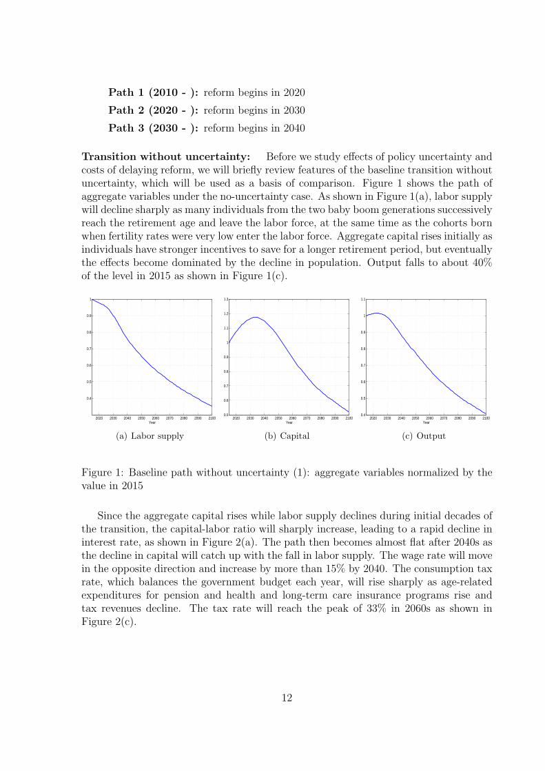
Transition without uncertainty: Before we study effects of policy uncertainty andcosts of delaying reform, we will briefly review features of the baseline transition withoutuncertainty, which will be used as a basis of comparison. Figure 1 shows the path ofaggregate variables under the no-uncertainty case. As shown in Figure 1(a), labor supplywill decline sharply as many individuals from the two baby boom generations successivelyreach the retirement age and leave the labor force, at the same time as the cohorts bornwhen fertility rates were very low enter the labor force. Aggregate capital rises initially asindividuals have stronger incentives to save for a longer retirement period, but eventuallythe effects become dominated by the decline in population. Output falls to about 40%of the level in 2015 as shown in Figure 1(c).
2020 2030 2040 2050 2060 2070 2080 2090 2100
0.4
0.5
0.6
0.7
0.8
0.9
1
Year
(a) Labor supply
2020 2030 2040 2050 2060 2070 2080 2090 21000.5
0.6
0.7
0.8
0.9
1
1.1
1.2
1.3
Year
(b) Capital
2020 2030 2040 2050 2060 2070 2080 2090 21000.4
0.5
0.6
0.7
0.8
0.9
1
1.1
Year
(c) Output
Figure 1: Baseline path without uncertainty (1): aggregate variables normalized by thevalue in 2015
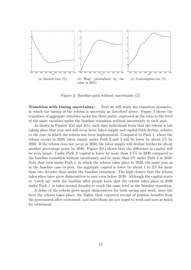
Since the aggregate capital rises while labor supply declines during initial decades ofthe transition, the capital-labor ratio will sharply increase, leading to a rapid decline ininterest rate, as shown in Figure 2(a). The path then becomes almost flat after 2040s asthe decline in capital will catch up with the fall in labor supply. The wage rate will movein the opposite direction and increase by more than 15% by 2040. The consumption taxrate, which balances the government budget each year, will rise sharply as age-relatedexpenditures for pension and health and long-term care insurance programs rise andtax revenues decline. The tax rate will reach the peak of 33% in 2060s as shown inFigure 2(c).
12
2010 2020 2030 2040 2050 2060 2070 2080 2090 21000
1
2
3
4
5
6
7
Year
(a) Interest rate (%)
2010 2020 2030 2040 2050 2060 2070 2080 2090 21000.95
1
1.05
1.1
1.15
1.2
1.25
Year
(b) Wage (normalized by thevalue in 2015)
2020 2030 2040 2050 2060 2070 2080 2090 21005
10
15
20
25
30
35
Year
(c) Consumption tax (%)
Figure 2: Baseline path without uncertainty (2)
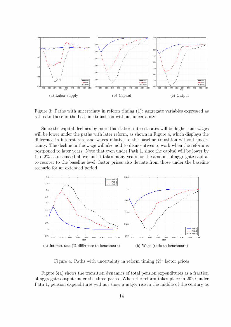
Transition with timing uncertainty: Next we will study the transition dynamics,in which the timing of the reform is uncertain as described above. Figure 3 shows thetransition of aggregate variables under the three paths, expressed as the ratio to the levelof the same variables under the baseline transition without uncertainty in each year.
As shown in Figures 3(a) and 3(b), each time individuals learn that the reform is nottaking place that year and will occur later, labor supply and capital both decline, relativeto the case in which the reform has been implemented. Compared to Path 1, where thereform occurs in 2020, labor supply under Path 2 and 3 will be lower by about 1% by2030. If the reform does not occur in 2030, the labor supply will decline further by aboutanother percentage point by 2040. Figure 3(b) shows that the difference in capital willbe even larger. Under Path 2, capital is lower by more than 3.5% in 2030 compared tothe baseline transition without uncertainty and by more than 6% under Path 3 in 2040.Note that even under Path 1, in which the reform takes place in 2020, the same year asin the baseline case ex-post, the aggregate capital is lower by about 1 to 2% for morethan two decades than under the baseline transition. The high chance that the reformtakes place later gives disincentives to save even before 2020. Although the capital startsto “catch up” with the baseline after people learn that the reform takes place in 2020under Path 1, it takes several decades to reach the same level as the baseline transition.
A delay of the reform gives major disincentives for both saving and work, since thelater the reform takes place, the higher their expected receipt of pension benefits fromthe government after retirement, and individuals are not urged to work and save as muchfor retirement.
13
2020 2030 2040 2050 2060 2070 2080 2090 21000.98
0.985
0.99
0.995
1
1.005
Year
Path 1Path 2Path 3
(a) Labor supply
2020 2030 2040 2050 2060 2070 2080 2090 21000.93
0.94
0.95
0.96
0.97
0.98
0.99
1
Year
Path 1Path 2Path 3
(b) Capital
2020 2030 2040 2050 2060 2070 2080 2090 21000.965
0.97
0.975
0.98
0.985
0.99
0.995
1
1.005
Year
Path 1Path 2Path 3
(c) Output
Figure 3: Paths with uncertainty in reform timing (1): aggregate variables expressed asratios to those in the baseline transition without uncertainty
Since the capital declines by more than labor, interest rates will be higher and wageswill be lower under the paths with later reform, as shown in Figure 4, which displays thedifference in interest rate and wages relative to the baseline transition without uncer-tainty. The decline in the wage will also add to disincentives to work when the reform ispostponed to later years. Note that even under Path 1, since the capital will be lower by1 to 2% as discussed above and it takes many years for the amount of aggregate capitalto recover to the baseline level, factor prices also deviate from those under the baselinescenario for an extended period.
2020 2030 2040 2050 2060 2070 2080 2090 2100−0.05
0
0.05
0.1
0.15
0.2
0.25
0.3
0.35
0.4
Year
Path 1Path 2Path 3
(a) Interest rate (% difference to benchmark)
2020 2030 2040 2050 2060 2070 2080 2090 21000.98
0.985
0.99
0.995
1
1.005
Year
Path 1Path 2Path 3
(b) Wage (ratio to benchmark)
Figure 4: Paths with uncertainty in reform timing (2): factor prices
Figure 5(a) shows the transition dynamics of total pension expenditures as a fractionof aggregate output under the three paths. When the reform takes place in 2020 underPath 1, pension expenditures will not show a major rise in the middle of the century as
14
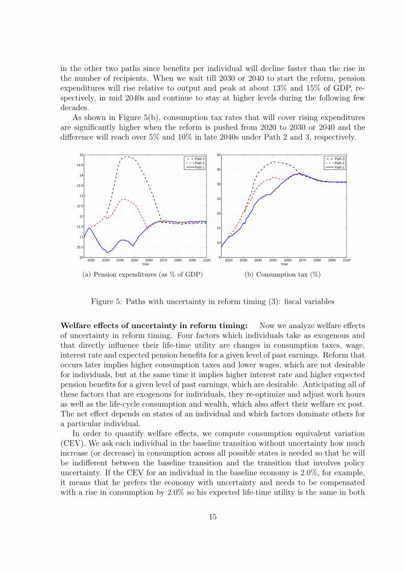
in the other two paths since benefits per individual will decline faster than the rise inthe number of recipients. When we wait till 2030 or 2040 to start the reform, pensionexpenditures will rise relative to output and peak at about 13% and 15% of GDP, re-spectively, in mid 2040s and continue to stay at higher levels during the following fewdecades.
As shown in Figure 5(b), consumption tax rates that will cover rising expendituresare significantly higher when the reform is pushed from 2020 to 2030 or 2040 and thedifference will reach over 5% and 10% in late 2040s under Path 2 and 3, respectively.
2020 2030 2040 2050 2060 2070 2080 2090 210010
10.5
11
11.5
12
12.5
13
13.5
14
14.5
15
Year
Path 3Path 2Path 1
(a) Pension expenditures (as % of GDP)
2020 2030 2040 2050 2060 2070 2080 2090 21005
10
15
20
25
30
35
40
Year
Path 3Path 2Path 1
(b) Consumption tax (%)
Figure 5: Paths with uncertainty in reform timing (3): fiscal variables
Welfare effects of uncertainty in reform timing: Now we analyze welfare effectsof uncertainty in reform timing. Four factors which individuals take as exogenous andthat directly influence their life-time utility are changes in consumption taxes, wage,interest rate and expected pension benefits for a given level of past earnings. Reform thatoccurs later implies higher consumption taxes and lower wages, which are not desirablefor individuals, but at the same time it implies higher interest rate and higher expectedpension benefits for a given level of past earnings, which are desirable. Anticipating all ofthese factors that are exogenous for individuals, they re-optimize and adjust work hoursas well as the life-cycle consumption and wealth, which also affect their welfare ex post.The net effect depends on states of an individual and which factors dominate others fora particular individual.
In order to quantify welfare effects, we compute consumption equivalent variation(CEV). We ask each individual in the baseline transition without uncertainty how muchincrease (or decrease) in consumption across all possible states is needed so that he willbe indifferent between the baseline transition and the transition that involves policyuncertainty. If the CEV for an individual in the baseline economy is 2.0%, for example,it means that he prefers the economy with uncertainty and needs to be compensatedwith a rise in consumption by 2.0% so his expected life-time utility is the same in both
15
economies. We compute the CEV for individuals at each age in the initial year of 2010and also for future generations. For the latter, the CEV is computed for a “new-born”individual at age 20 who just enter the economy and for each possible transition paththat can be realized.
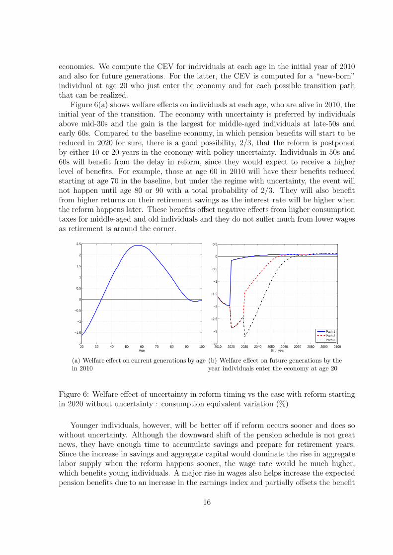
Figure 6(a) shows welfare effects on individuals at each age, who are alive in 2010, theinitial year of the transition. The economy with uncertainty is preferred by individualsabove mid-30s and the gain is the largest for middle-aged individuals at late-50s andearly 60s. Compared to the baseline economy, in which pension benefits will start to bereduced in 2020 for sure, there is a good possibility, 2/3, that the reform is postponedby either 10 or 20 years in the economy with policy uncertainty. Individuals in 50s and60s will benefit from the delay in reform, since they would expect to receive a higherlevel of benefits. For example, those at age 60 in 2010 will have their benefits reducedstarting at age 70 in the baseline, but under the regime with uncertainty, the event willnot happen until age 80 or 90 with a total probability of 2/3. They will also benefitfrom higher returns on their retirement savings as the interest rate will be higher whenthe reform happens later. These benefits offset negative effects from higher consumptiontaxes for middle-aged and old individuals and they do not suffer much from lower wagesas retirement is around the corner.
20 30 40 50 60 70 80 90 100−2
−1.5
−1
−0.5
0
0.5
1
1.5
2
2.5
Age
(a) Welfare effect on current generations by agein 2010
2010 2020 2030 2040 2050 2060 2070 2080 2090 2100−3.5
−3
−2.5
−2
−1.5
−1
−0.5
0
0.5
Birth year
Path 1Path 2Path 3
(b) Welfare effect on future generations by theyear individuals enter the economy at age 20
Figure 6: Welfare effect of uncertainty in reform timing vs the case with reform startingin 2020 without uncertainty : consumption equivalent variation (%)
Younger individuals, however, will be better off if reform occurs sooner and does sowithout uncertainty. Although the downward shift of the pension schedule is not greatnews, they have enough time to accumulate savings and prepare for retirement years.Since the increase in savings and aggregate capital would dominate the rise in aggregatelabor supply when the reform happens sooner, the wage rate would be much higher,which benefits young individuals. A major rise in wages also helps increase the expectedpension benefits due to an increase in the earnings index and partially offsets the benefit
16
reduction due to the reform. Lower consumption tax when the reform happens sooneralso helps during long remaining years of their life.
These observations also apply for individuals who enter the economy in future asshown in Figure 6(b). A further delay of the reform implies an even larger loss relativeto the transition with no reform uncertainty. Even under Path 1, where, ex post, thepolicy is the same as in the baseline transition and the reform starts in 2020, the welfareloss can amount to a negative 2% in consumption equivalence for generations that enterthe economy in around 2020. Those who enter the economy in 2030 and find the reformoccur at the latest timing of 2040 would be significantly worse off and the welfare lossamounts to more than 3% in CEV.
The analysis demonstrates a stark welfare tradeoff across generations through a delayin pension reform. Pushing the timing of reform as far as possible is in the interest ofmiddle and old-aged individuals but it comes with deteriorating welfare of young andfuture generations.
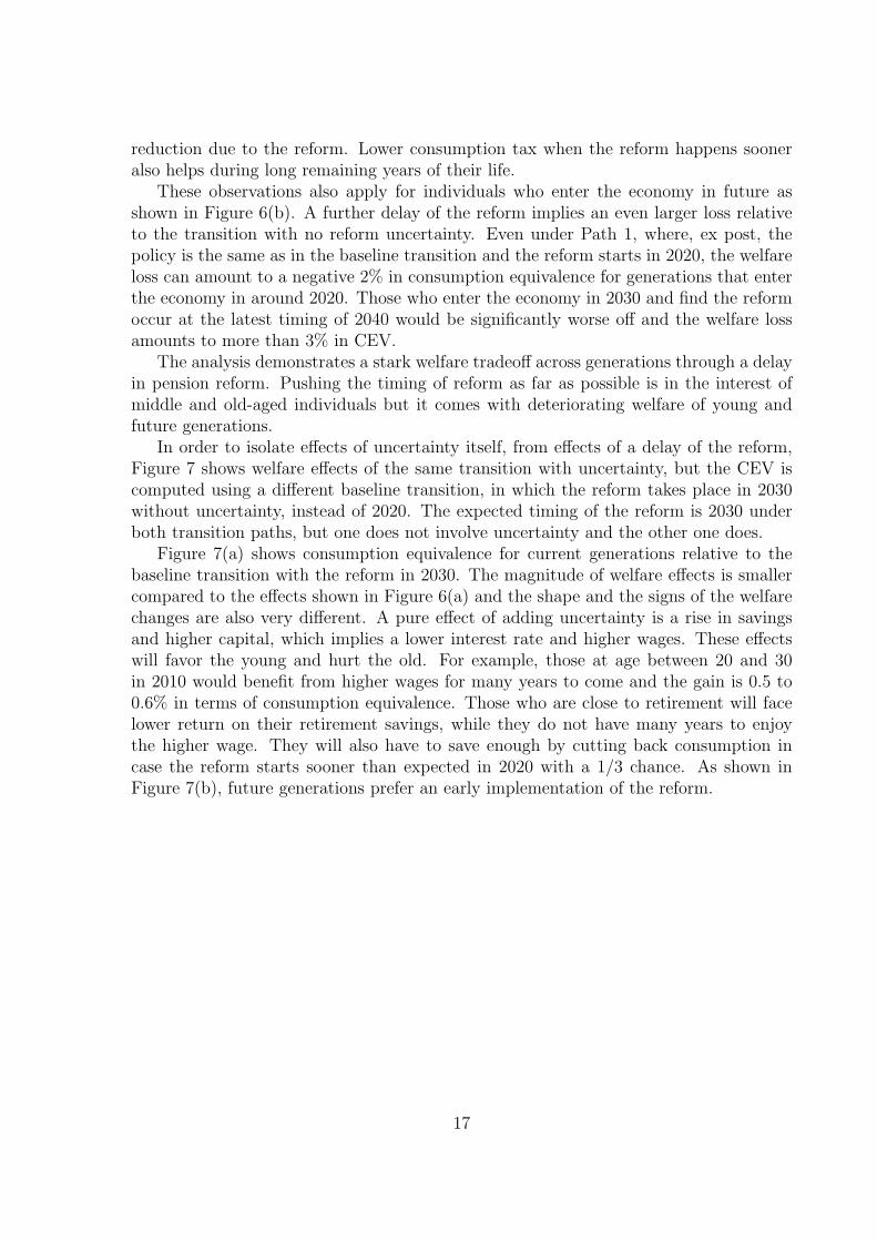
In order to isolate effects of uncertainty itself, from effects of a delay of the reform,Figure 7 shows welfare effects of the same transition with uncertainty, but the CEV iscomputed using a different baseline transition, in which the reform takes place in 2030without uncertainty, instead of 2020. The expected timing of the reform is 2030 underboth transition paths, but one does not involve uncertainty and the other one does.
Figure 7(a) shows consumption equivalence for current generations relative to thebaseline transition with the reform in 2030. The magnitude of welfare effects is smallercompared to the effects shown in Figure 6(a) and the shape and the signs of the welfarechanges are also very different. A pure effect of adding uncertainty is a rise in savingsand higher capital, which implies a lower interest rate and higher wages. These effectswill favor the young and hurt the old. For example, those at age between 20 and 30in 2010 would benefit from higher wages for many years to come and the gain is 0.5 to0.6% in terms of consumption equivalence. Those who are close to retirement will facelower return on their retirement savings, while they do not have many years to enjoythe higher wage. They will also have to save enough by cutting back consumption incase the reform starts sooner than expected in 2020 with a 1/3 chance. As shown inFigure 7(b), future generations prefer an early implementation of the reform.
17
20 30 40 50 60 70 80 90 100−0.8
−0.6
−0.4
−0.2
0
0.2
0.4
0.6
Age
(a) Welfare effect on current generations by agein 2010
2010 2020 2030 2040 2050 2060 2070 2080 2090 2100−2
−1.5
−1
−0.5
0
0.5
1
1.5
2
Birth year
Path 1Path 2Path 3
(b) Welfare effect on future generations by theyear individuals enter the economy at age 20
Figure 7: Welfare effect of uncertainty in reform timing vs the case with reform startingin “2030” without uncertainty : consumption equivalent variation (%)
4.2 Uncertainty in reform timing and policy
Next we consider a different form of uncertainty, in which the final pension scheme isuncertain. On top of the three paths we studied above, we add a scenario in whichthere is in fact no reform to reduce the benefits beyond 20% as embedded in the 2004pension reform. There is a reduction, but under this scenario benefits are reduced in amuch smaller scale compared to the scenario to cut them by 36%. As before, there arethree possible timings of the reform in 2020, 2030 and 2040 and to these we add anotherscenario in which benefits are reduced by only 20% in the end.
If no reform has occurred in 2020 or 2030, individuals will learn in 2040 whether thereis reform in that year or not. We call the transition path under the latter scenario asPath 4, in which there is no aggressive reform and benefits will be reduced only by 20%rather than 36%, starting in 2040.
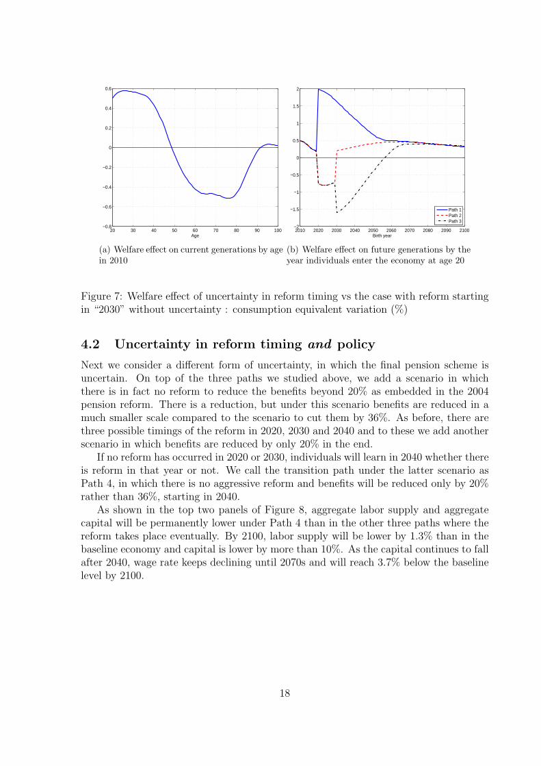
As shown in the top two panels of Figure 8, aggregate labor supply and aggregatecapital will be permanently lower under Path 4 than in the other three paths where thereform takes place eventually. By 2100, labor supply will be lower by 1.3% than in thebaseline economy and capital is lower by more than 10%. As the capital continues to fallafter 2040, wage rate keeps declining until 2070s and will reach 3.7% below the baselinelevel by 2100.
18
2020 2030 2040 2050 2060 2070 2080 2090 21000.975
0.98
0.985
0.99
0.995
1
1.005
Year
Path 1Path 2Path 3Path 4
(a) Labor supply
2020 2030 2040 2050 2060 2070 2080 2090 21000.88
0.9
0.92
0.94
0.96
0.98
1
Year
Path 1Path 2Path 3Path 4
(b) Capital
2020 2030 2040 2050 2060 2070 2080 2090 2100−0.1
0
0.1
0.2
0.3
0.4
0.5
0.6
0.7
0.8
Year
Path 1Path 2Path 3Path 4
(c) Interest rate
2020 2030 2040 2050 2060 2070 2080 2090 21000.96
0.965
0.97
0.975
0.98
0.985
0.99
0.995
1
1.005
Year
Path 1Path 2Path 3Path 4
(d) Wage
Figure 8: Paths with uncertainty in timing and policy (1): aggregate variables expressedas ratios to the benchmark without uncertainty except for the interest rate which isexpressed as difference in percentage points.
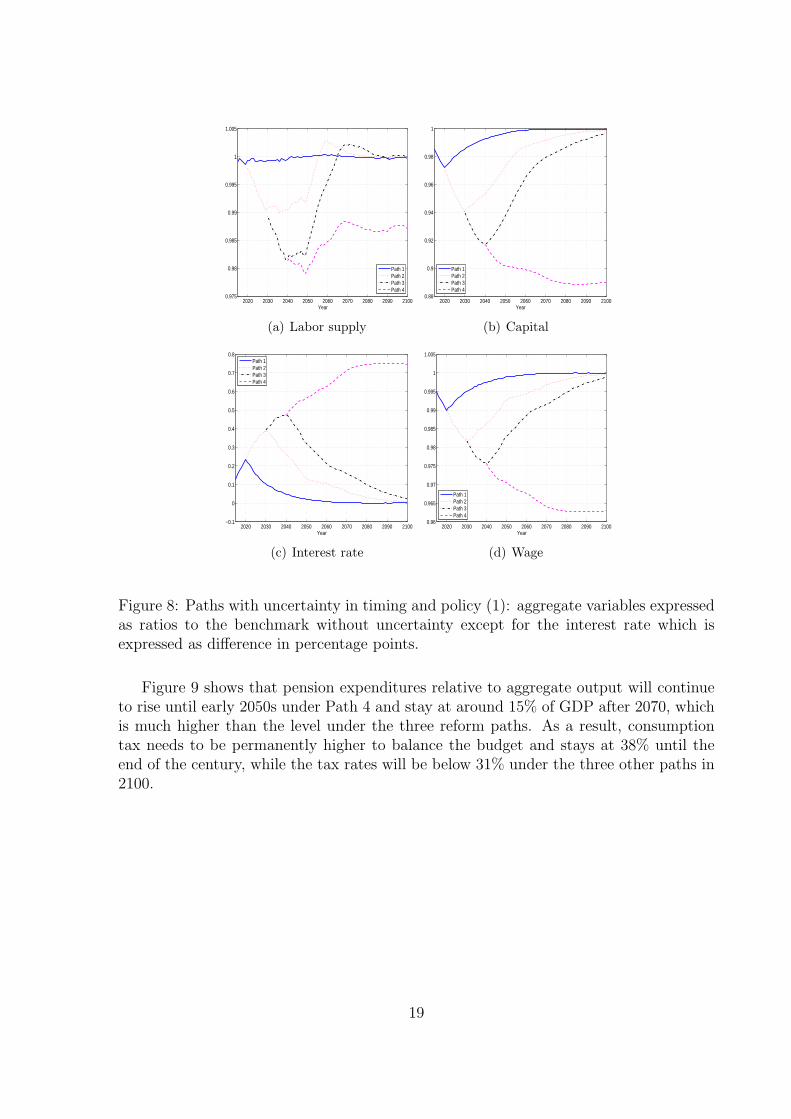
Figure 9 shows that pension expenditures relative to aggregate output will continueto rise until early 2050s under Path 4 and stay at around 15% of GDP after 2070, whichis much higher than the level under the three reform paths. As a result, consumptiontax needs to be permanently higher to balance the budget and stays at 38% until theend of the century, while the tax rates will be below 31% under the three other paths in2100.
19
2010 2020 2030 2040 2050 2060 2070 2080 2090 21009
10
11
12
13
14
15
16
17
Year
Path 4Path 3Path 2Path 1
(a) Pension expenditures (as % of GDP)
2010 2020 2030 2040 2050 2060 2070 2080 2090 21000
5
10
15
20
25
30
35
40
45
Year
(b) Consumption tax (%)
Figure 9: Paths with uncertainty in timing and policy (2): fiscal variables
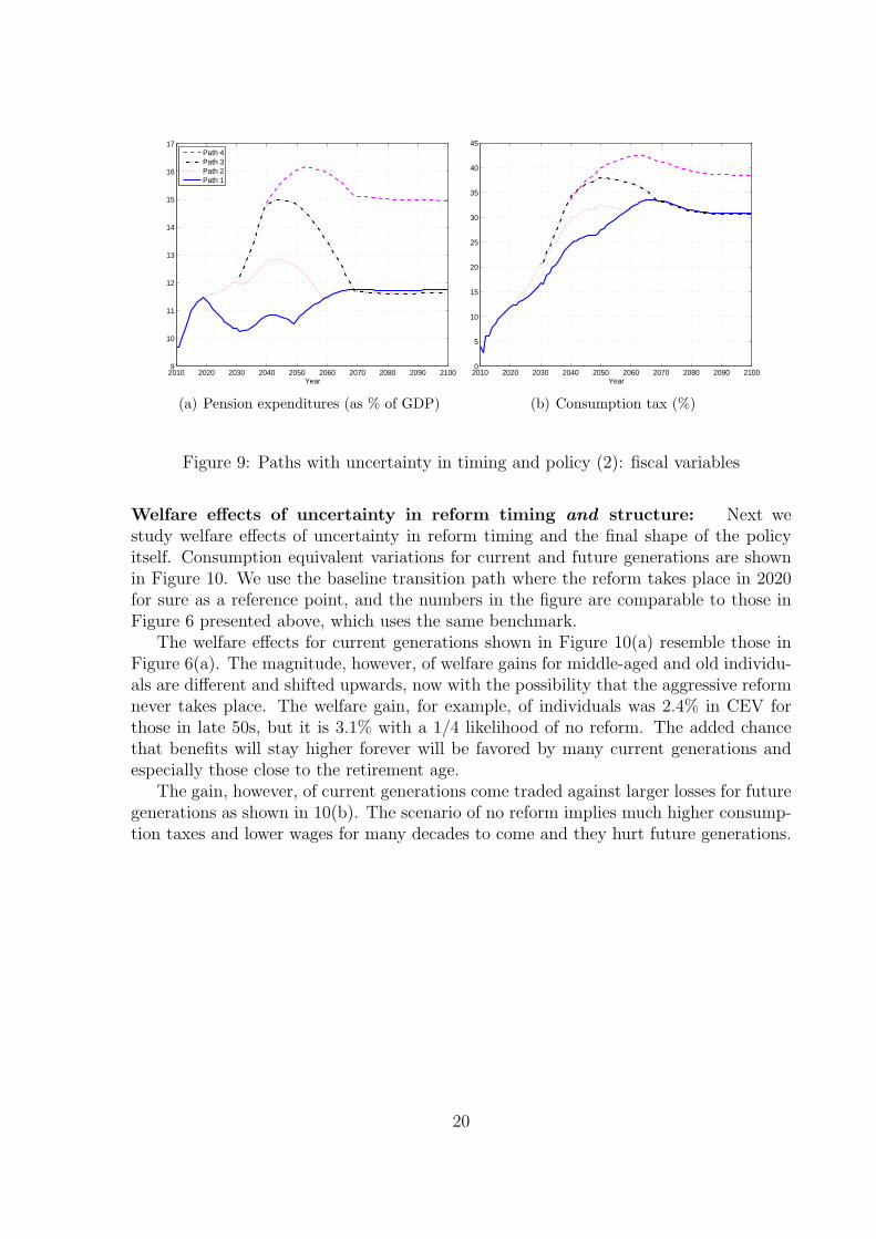
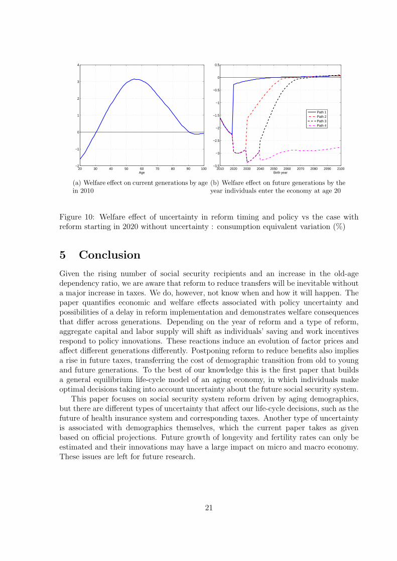
Welfare effects of uncertainty in reform timing and structure: Next westudy welfare effects of uncertainty in reform timing and the final shape of the policyitself. Consumption equivalent variations for current and future generations are shownin Figure 10. We use the baseline transition path where the reform takes place in 2020for sure as a reference point, and the numbers in the figure are comparable to those inFigure 6 presented above, which uses the same benchmark.
The welfare effects for current generations shown in Figure 10(a) resemble those inFigure 6(a). The magnitude, however, of welfare gains for middle-aged and old individu-als are different and shifted upwards, now with the possibility that the aggressive reformnever takes place. The welfare gain, for example, of individuals was 2.4% in CEV forthose in late 50s, but it is 3.1% with a 1/4 likelihood of no reform. The added chancethat benefits will stay higher forever will be favored by many current generations andespecially those close to the retirement age.
The gain, however, of current generations come traded against larger losses for futuregenerations as shown in 10(b). The scenario of no reform implies much higher consump-tion taxes and lower wages for many decades to come and they hurt future generations.
20
20 30 40 50 60 70 80 90 100−2
−1
0
1
2
3
4
Age
(a) Welfare effect on current generations by agein 2010
2010 2020 2030 2040 2050 2060 2070 2080 2090 2100−3.5
−3
−2.5
−2
−1.5
−1
−0.5
0
0.5
Birth year
Path 1Path 2Path 3Path 4
(b) Welfare effect on future generations by theyear individuals enter the economy at age 20
Figure 10: Welfare effect of uncertainty in reform timing and policy vs the case withreform starting in 2020 without uncertainty : consumption equivalent variation (%)
5 Conclusion
Given the rising number of social security recipients and an increase in the old-agedependency ratio, we are aware that reform to reduce transfers will be inevitable withouta major increase in taxes. We do, however, not know when and how it will happen. Thepaper quantifies economic and welfare effects associated with policy uncertainty andpossibilities of a delay in reform implementation and demonstrates welfare consequencesthat differ across generations. Depending on the year of reform and a type of reform,aggregate capital and labor supply will shift as individuals’ saving and work incentivesrespond to policy innovations. These reactions induce an evolution of factor prices andaffect different generations differently. Postponing reform to reduce benefits also impliesa rise in future taxes, transferring the cost of demographic transition from old to youngand future generations. To the best of our knowledge this is the first paper that buildsa general equilibrium life-cycle model of an aging economy, in which individuals makeoptimal decisions taking into account uncertainty about the future social security system.
This paper focuses on social security system reform driven by aging demographics,but there are different types of uncertainty that affect our life-cycle decisions, such as thefuture of health insurance system and corresponding taxes. Another type of uncertaintyis associated with demographics themselves, which the current paper takes as givenbased on official projections. Future growth of longevity and fertility rates can only beestimated and their innovations may have a large impact on micro and macro economy.These issues are left for future research.
21
References
Attanasio, O. P., S. Kitao, and G. L. Violante (2007). Global demographics trendsand Social Security reform. Journal of Monetary Economics 54 (1), 144–198.
Auerbach, A. J. and K. A. Hassett (2002). Fiscal policy and uncertainty. InternationalFinance 5 (2), 229–249.
Auerbach, A. J. and K. A. Hassett (2007). Optimal long-run fiscal policy: Constraints,preferences and the resolution of uncertainty. Journal of Economic Dynamics andControl 31, 1451–1472.
Auerbach, A. J. and L. J. Kotlikoff (1987). Dynamic Fiscal Policy. Cambridge: Cam-bridge University Press.
Baker, S. R., N. Bloom, and S. J. Davis (2015). Measuring economic policy uncertainty.NBER Working Paper 21633.
Bi, H., E. M. Leeper, and C. Leith (2013). Uncertain fiscal consolidations. EconomicJournal 123, 31–63.
Braun, A. R. and D. H. Joines (2015). The implications of a graying Japan for gov-ernment policy. Journal of Economic Dynamics and Control 57, 1–23.
Butler, M. (1999). Anticipation effects of looming public-pension reforms. Carnegie-ROchester Conference Series on Public Policy 50, 119–159.
Caliendo, F. N., A. Gorry, and S. Slavov (2015). The cost of uncertainty about thetiming of social security reform. Working Paper.
Conesa, J. C. and D. Krueger (1999). Social Security with heterogeneous agents. Re-view of Economic Dynamics 2 (4), 757–795.
De Nardi, M., S. Imrohoroglu, and T. J. Sargent (1999). Projected U.S. demographicsand social security. Review of Economic Dynamics 2 (3), 575–615.
Fernandez-Villaverde, J., P. Guerron-Quintana, K. Kuester, and J. Rubio-Ramırez(2013). Fiscal volatility shocks and economic activity. Working Paper.
Gomes, F. J., L. J. Kotlikoff, and L. M. Viceira (2012). The excess burden of gov-ernment indecision. In J. Brown (Ed.), Tax Policy and the Economy, Volume 26,Chapter 5, pp. 125–163. Chicago: University of Chicago Press.
Hansen, G. D. and S. Imrohoroglu (2013). Fiscal reform and government debt in Japan:A neoclassical perspective. NBER Working Paper 19431.
Hayashi, F. and E. C. Prescott (2002). The 1990s in Japan: A lost decade. Review ofEconomic Dynamics 5 (1), 206–235.
Huggett, M. and G. Ventura (1999). On the distributional effects of social securityreform. Review of Economic Dynamics 2 (3), 498– 531.
Imrohoroglu, A., S. Imrohoroglu, and D. Joines (1995). A life cycle analysis of socialsecurity. Economic Theory 6 (1), 83–114.
22
Imrohoroglu, S. and S. Kitao (2012). Social Security reforms: Benefit claiming, la-bor force participation and long-run sustainability. American Economic Journal:Macroeconomics 4 (3), 96–127.
Imrohoroglu, S., S. Kitao, and T. Yamada (2015). Can guest workers solve japan’sfiscal problems? Working Paper.
Kitao, S. (2014). Sustainable Social Security: Four options. Review of Economic Dy-namics 17 (4), 756–779.
Kitao, S. (2015a). Fiscal cost of demographic transition in Japan. Journal of EconomicDynamics and Control 54, 37–58.
Kitao, S. (2015b). Pension reform and Individual Retirement Accounts in Japan. Jour-nal of The Japanese and International Economies 38, 111–126.
Luttmer, E. F. P. and A. A. Samwick (2015). The welfare cost of perceived policyuncertainty: Evidence from social security. Working Paper.
Nishiyama, S. and K. Smetters (2007). Does Social Security privatization produceefficiency gains? Quarterly Journal of Economics 122 (4), 1677–1719.
23