Embed Size (px)
Citation preview

1750 Massachusetts Avenue, NW | Washington, DC 20036-1903 USA | 202.328.9000 Tel | 202.328.5432 Fax | www.piie.com
POLICY BRIEF
17-19 Estimatesof FundamentalEquilibriumExchange Rates,May 2017William R. ClineMay 2017 Revised June 2017
William R. Cline, senior fellow, has been associated with the Peterson Institute for International Economics since its incep-tion in 1981. His numerous publications include Managing the Euro Area Debt Crisis (2014), Financial Globalization, Economic Growth, and the Crisis of 2007–09 (2010), and The United States as a Debtor Nation (2005).
Author’s Note: I thank Fredrick Toohey for research assis-tance. For comments on an earlier draft, I thank without impli-cating Joseph Gagnon, Egor Gornostay, Trevor Houser, Gary Hufbauer, and Ted Truman.
© Peterson Institute for International Economics. All rights reserved.
In the first few months of the Trump administration, the strong dollar has eased slightly rather than surging further. Potentially destabilizing dynamics associated with fiscal stimulus and trade policy confrontations have been at least delayed. Nonetheless, underlying upward pressure on the dollar seems likely to persist as the United States moves toward monetary normalization on a faster track than the euro area and Japan. Moreover, the leading congressional proposal for corporate tax reform includes a border tax adjustment that could push the dollar sharply upward, even though the move would likely be considerably smaller and slower than many economists predict. Although strong opposition from import-oriented business sectors makes it unlikely that the proposed border tax will be adopted, especially in view of its conspicuous absence in the tax reform plans announced by
the Trump administration on April 26, some variant of the tax could resurface in legislative negotiations.1
This Policy Brief provides updated estimates of funda-mental equilibrium exchange rates (FEERs).2 The new estimates once again find that the most important currency misalignment is that of the US dollar, which would need to depreciate by about 8 percent to be consistent with its FEER. Before turning to the updated estimates for the United States and other major economies, it is important to take stock of the political and monetary forces presently driving the environment for exchange rates.
MODERATING TRADE AND CURRENCY CONFLICT IN THE NEW US ADMINISTRATION
The potential for trade and currency conflict that had marked Donald Trump’s presidential campaign has largely been avoided in the first few months of his administration. Trump had made a major campaign pledge that on “day one” he would declare China to be a currency manipula-tor.3 Instead, in mid-April he stated that his administration would not designate China as a currency manipulator. He indicated that he had changed his mind because China had not been manipulating its currency for months and because he did not want to jeopardize discussions with China in dealing with the threat from North Korea.4 In its semian-
1. Sam Fleming and Barney Jopson, “The unanswered ques-tions in Trump’s tax plan,” Financial Times, April 27, 2017.
2. First introduced in Cline and Williamson (2008), the semi-annual calculations of fundamental equilibrium exchangerates (FEERs) examine the extent to which exchange ratesneed to change in order to curb any prospectively excessivecurrent account imbalances back to a limit of ±3 percentof GDP. This target range is intended to be consistent withsustainability for deficit countries and global adding-up forsurplus countries. The estimates apply the Symmetric MatrixInversion Method (SMIM) model (Cline 2008). For a sum-mary of the methodology, see Cline and Williamson (2012,appendix A), available at http://www.piie.com/publications/pb/pb12-14.pdf (accessed on May 24, 2017).
3. See e.g. Doug Palmer and Ben Schreckinger, “Trumpvows to declare China a currency manipulator on Day One,”Politico, November 10, 2015.
4. Gerard Baker, Carol E. Lee, and Michael C. Bender, “Trump

2 3
May 2017
nual report on exchange rates released soon thereafter, the US Treasury Department found that “no major trading partner met all three criteria [for currency manipulation] for the current reporting period” (Treasury 2017, 1).5 It was widely known that the charge of Chinese manipulation was outdated. Since mid-2014 China’s reserves have fallen from $4 trillion to $3 trillion as it has sought to keep the renminbi from falling in the face of capital outflows, the opposite of manipulative intervention to keep the currency artificially cheap (see appendix A for further discussion). Nor did the new administration implement the campaign threat to impose a 45 percent tariff on China.6 Instead, following an amicable summit with Chinese president Xi Jinping, the administration indicated it would draft a 100-day plan to address bilateral trade disputes.7
Similarly, candidate Trump had threatened a 35 percent tariff against Mexico, reflecting his demand that Mexico pay for a border wall and his view that the North American Free Trade Agreement (NAFTA) had been a disastrous trade agreement for the United States.8 Instead, by February, US and Mexican negotiators appeared to be moving toward a more orthodox process of renegotiating the agreement.9 At the end of April Trump announced he would not withdraw the United States from NAFTA but would renegotiate it.10
Says Dollar ‘Getting Too Strong,’ Won’t Label China a Currency Manipulator,” Wall Street Journal, April 12, 2017.
5. The three criteria are: bilateral trade surplus of at least $20 billion with the United States, current account surplus of at least 3 percent of GDP, and one-sided intervention accumu-lating at least 2 percent of GDP in additional reserves over 12 months. The report did emphasize, however, that: “China has a long track record of engaging in persistent, large-scale, one-way foreign exchange intervention, doing so for roughly a decade to resist renminbi (RMB) appreciation even as its trade and current account surpluses soared.” Treasury 2017, 2.
6. Maggie Haberman, “Donald Trump Says He Favors Big Tariffs on Chinese Exports,” New York Times, January 7, 2016.
7. Clay Chandler, “The Trump-Xi Summit Was a Showdown that Wasn’t,” Forbes, April 10, 2017.
8. The 35 percent tax was typically stated in connection with discouraging firms from moving manufacturing to Mexico. See for example Patrick Gillespie, “Trump’s 35% Mexico tax would cost Ford billions and hurt Americans,” CNNMoney, September 15, 2016.
9. Thus, consultations with the private sector reportedly began in February (Ana Swanson and Joshua Partlow, “U.S. and Mexico appear to take first steps toward renegotiating NAFTA, document suggests,” Washington Post, February 1, 2017). By late March, a draft letter setting forth the admin-istration’s renegotiation goals featured “a much more mea-sured tone” than that of the campaign (Michael Grunwald, “For Trump, NAFTA Could Be the Next Obamacare,” Politico, April 4, 2017).
10. Binyamin Appelbaum and Glenn Thrush, “Trump’s Day
Reflecting the seeming reversal from intense confrontation toward business as usual, the Mexican peso rebounded sharply from its lows shortly before Trump took office.11
Although early and massive trade conflict with China and Mexico has been avoided, by late April the Trump administration began proceedings for potential sectoral protection in steel (on national security grounds) and on lumber imports from Canada.12 Trump has also been critical of persistent US trade deficits and has complained that the dollar is too strong for competitiveness.13 The political envi-ronment thus remains susceptible to rising trade tensions if the trade deficit widens further.
US TAX CUTS AND POTENTIAL FISCAL PRESSURES
At the end of April the Trump administration announced the outlines of its tax reform program.14 The corporate tax rate would be cut from 35 percent to 15 percent and would shift to a territorial basis that excludes foreign profits. Passthrough entities would shift from taxation at the recipient’s personal rate to the corporate rate.15 Personal tax brackets would be cut from seven to three, with the top rate cut from 39.6 percent to 35 percent. Deductions would be
of Hardball and Confusion on Nafta,” New York Times, April 27, 2017. In mid-May, the administration formally notified Congress of its intention to renegotiate NAFTA (Julie Hirschfeld Davis, “Trump Sends Nafta Renegotiation Notice to Congress,” New York Times, May 18, 2017).
11. From the end of October 2015 to the end of October 2016, the peso fell 12.5 percent against the dollar, even though Mexico’s rate of inflation was only 0.6 percent higher than US inflation. After the surprise victory of Mr. Trump, the peso fell an additional 13.7 percent to its trough of 21.9 per dollar on January 11, 2017. Thereafter the peso rebounded 16 percent by mid-April, returning to its end-October level of about 18.8 pesos per dollar. Bloomberg; IMF 2017a.
12. Chad Bown, “Trump’s threat of steel tariffs heralds big changes in trade policy,” Washington Post, April 21, 2017; Peter Baker and Ian Austen, “In New Trade Front, Trump Slaps Tax on Canadian Lumber,” New York Times, April 24, 2017.
13. Gavyn Davies, “President Trump abandons the strong dol-lar policy,” Financial Times, April 15, 2017. On trade deficits, Trump has stated: “The jobs and wealth have been stripped from our country year after year, decade after decade, trade deficit upon trade deficit.” Shawn Donnan and Tom Mitchell, “Trump demands solution to US trade deficits with China and others,” Financial Times, March 31, 2017.
14. Julie Hirschfeld Davis and Alan Rappeport, “White House Proposes Slashing Tax Rates, Significantly Aiding Wealthy,” New York Times, April 26, 2017.
15. Subchapter S corporations and limited liability partner-ships provide corporate limitation of liability, but their income is presently taxed at the individual recipient’s rate rather than the corporate rate.

2 3
May 2017
16. “Fiscal FactCheck: How Much Will Trump’s Tax PlanCost?” Committee for a Responsible Federal Budget, April26, 2017. Available at www.crfb.org/blogs/fiscal-factcheck-how-much-will-trumps-tax-plan-cost (accessed on May 24,2017).
17. Calculated from CBO 2017a, assuming a cumulative rev-enue loss of $5.5 trillion.
18. See the April 26 press conference with TreasurySecretary Steve Mnuchin and National Economic DirectorGary Cohn, available at https://www.youtube.com/watch?v=n0MTxp1gFpo (accessed on May 24, 2017). Notethat in comparison, baseline economic growth is projectedat 1.8 percent. Supplementary tables available at https://www.cbo.gov/about/products/budget-economic-data#4(accessed on May 24, 3017).
19. Calculated from CBO 2017b baselines for real growth andGDP deflator inflation.
relatively slow growth of the labor force (0.4 percent in the CBO projections; CBO 2017b, 30).20 Overall, even though the announced plan may be more of an opening bargaining position than a realistic plan, the prospect of unfunded tax cuts heightens the outlook for larger fiscal deficits, higher interest rates, and as a result a stronger dollar going forward.
RELATIVE MONETARY CONDITIONS AND THE EXCHANGE RATE
The already strong dollar means that larger current account deficits are already in the pipeline. As shown in appendix figure A.1, the real effective exchange rate of the dollar has recently been at its strongest level of the past decade. The real dollar is only about 9 percent below its most recent peak in October 2002, although it is still 20 percent below its record level in March 1985. Moreover, the move toward monetary normalization in the United States, well ahead of that in the euro area and Japan, seems likely to push the dollar higher, especially if even faster increases in interest rates are forced by fiscal expansion from tax cuts and infra-structure spending.
How differential monetary stances have influenced the exchange rate of the dollar against the two other leading international currencies, the euro and the yen, in recent years provides insight into the extent to which relative US monetary tightening might further strengthen the dollar. For both currencies, it turns out that the differential in the long-term interest rate does a relatively good job in explaining the path of the exchange rate against the dollar in recent years. The long-term government bond rate fell more steeply in the United States and Germany than in Japan from 2007 to 2012 (figure 1), contributing to the rise in the yen in this period. Then the rate broadly stabilized in the United States but continued to decline toward zero in both Germany and Japan, helping to explain the rise in the dollar relative to both.
Simple statistical regressions using the interest differen-tial as the sole explanatory variable (or, in the case of Japan, including a dummy variable for prime minister Shinzo Abe’s economic policies, Abenomics, in 2013 and after) yield
20. The Tax Foundation estimates that cutting the corporatetax from 35 to 15 percent could boost the growth rate by 0.4percent per year over a decade, but calculates that the extrarevenue from higher growth would cover less than half of therevenue loss. In contrast, the Tax Policy Center estimates thatthe final tax reform plan in the Trump campaign would pro-vide no additional growth at all in the first decade, and wouldcause slower growth thereafter as a consequence of higherinterest rates from higher debt. For the first decade, the TaxPolicy Center estimates a cumulative revenue loss of $6.2trillion. See Alan Cole, “Could Trump’s Corporate Rate Cut to15 Percent be Self-Financing?” Tax Foundation, April 25, 2017;and Howard Gleckman, “Trump’s Familiar Tax Plan WouldAdd Trillions to the Debt,” Tax Policy Center, April 26, 2017.
Number PB17-19
limited to charitable contributions, home mortgage interest, and retirement contributions (thereby eliminating deduc-tion of state and local taxes). The standard deduction would be doubled to $24,000 for couples filing jointly. The alter-native minimum tax, estate tax, and healthcare surcharge on capital income would be eliminated.
One leading center estimates the net revenue losses from the tax reform at $5.5 trillion over 10 years.16 The Congressional Budget Office (CBO 2017a, 10) projects cumulative nominal GDP at $237 trillion over this period, so the direct loss would be 2.3 percent of GDP. In effect, the revenue from corporate, personal, and other taxes except for payroll taxes (dedicated to Social Security) would fall from an average of about 12 percent of GDP to about 10 percent of GDP.17 US Treasury Secretary Steven Mnuchin indi-cated that faster growth averaging 3 percent would bring in enough revenue to make the cuts self-financing.18
The prospect of unfunded tax cuts heightens the outlook for larger fiscal deficits, higher interest rates, and as a result a stronger dollar going forward.
However, with baseline growth averaging 1.8 percent, even if 3 percent growth were achieved, it is unlikely the extra revenue would be sufficient to cover the revenue loss. If the new, lower 10 percent rate (excluding payroll taxes) is simply applied to the extra nominal income from the extra growth, the net revenue loss would still be $3.3 tril-lion. Even if the elasticity of revenue with respect to GDP were 2, the net revenue loss would still amount to $2.1 tril-lion.19 More fundamentally, the incentive effects from the tax reform are not likely to be sufficient to raise the average rate of labor productivity growth from 1.5 percent annu-ally to 2.6 percent, which would be necessary in view of the

4 5
May 2017
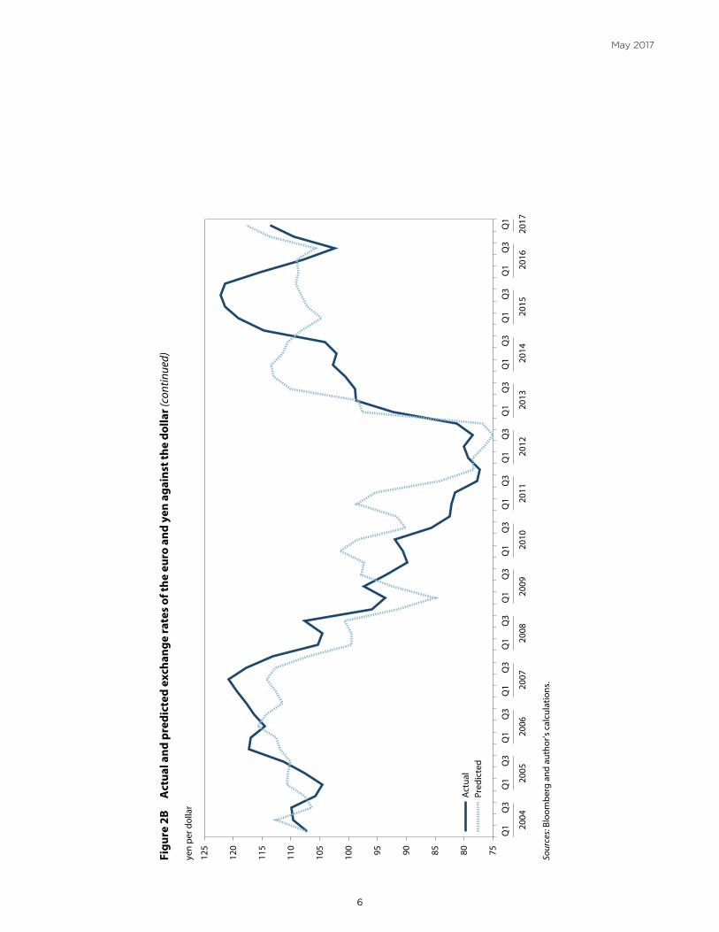
relatively good explanations for the exchange rates against the dollar for this period.21 Figure 2 shows the actual and predicted paths of the euro and yen against the dollar based on the statistical relationships to the interest differential.22
In these statistical results, an extra 100 basis points in the difference between the long-term government bond rate for the United States and that for Germany causes a decline of 14.6 US cents per euro (dollar appreciation). A 100 basis point increase in the differential against the long-term rate for Japan causes the number of yen per dollar to rise by 17.4 (dollar appreciation). Tests using the change from the previous quarter for exchange rates and interest differentials, rather than quarterly average levels, yield somewhat smaller but still statistically significant coefficients.23
21. Thus: With r as the long-term interest rate, and subscripts G, J, and U indicating Germany, Japan, and the United States, estimates are: 1) $/€ = 1.398 (99) + 0.146 × [rG-rU] (10); adj. R2 = 0.67, for dollars per euro; and 2) ¥/$ = 60.4 (15) + 17.4 × [rU-rJ] (10) + 16.0 D (6.8); adj. R2 = 0.69, for the yen, where D = 0 through 2012 and 1 thereafter. T-statistics are in paren-theses. Data are quarterly averages through 2017:1, beginning in 2005:1 for the euro and 2004:1 for the yen.
22. In its initial years (and especially 2000–2002), the euro was weaker against the dollar than would have been predicted by the model in figure 2. This period included an early phase of adjustment to increased supply of euro-denominated debt, as well as a period of strong capital flows into the US equity market. See Meredith 2001.
23. In these first-difference regressions, the coefficient on the
Because the United States is further along in the process of normalizing its monetary policy than either the euro area or Japan, further increases in US interest rates relative to those in Germany and Japan might be expected in the next two or three years. Market forecasts of long-term interest rates provide a basis for examining the potential for further dollar appreciation against the two currencies. As of March 2017, the median private forecast for the 10-year govern-ment rate for 2018 was 3.2 percent for the United States (Blue Chip 2017), compared to 0.7 percent for Germany and 0.1 percent for Japan (Consensus 2017). The US interest differential would thus stand at 2.5 percent against Germany and 3.1 percent against Japan.
The models of figure 2 accordingly project the 2018 exchange rates at 1.033 dollars per euro and 130.4 yen per dollar. Application of the smaller coefficients from the first-difference regressions place the estimated exchange rates for 2018 at 1.016 dollars per euro and 118.7 yen per dollar.24 Compared to average rates in the first quarter of 2017, these rates amount to dollar appreciations of about 3 to 5 percent
interest rate differential narrows from 0.146 to 0.120 (2.8) for the euro, and from 17.4 to 6.9 (3.2) for the yen (t-statistics in parentheses).
24. The implied forecasts apply the equation-estimated level of the exchange rate in 2017:1 as the base, for the “levels” re-gressions, and the actual 2017:1 levels of the exchange rates as the base for the first-difference regressions.
Figure 1 Long-term government bond rates: United States, Germany, and Japan
Note: 2017 refers to January–February.Source: IMF 2017a.
–1
0
1
2
3
4
5
6
2004 2005 2006 2007 2008 2009 2010 2011 2012 2013 2014 2015 2016 2017
percent
GermanyJapan
United States

4 5
May 2017
Figu
re 2
A
Act
ual a
nd p
redi
cted
exc
hang
e ra
tes
of th
e eu
ro a
nd y
en a
gain
st th
e do
llar
1.0
1.1
1.2
1.3
1.4
1.5
1.6
2005
Q1
Q3
2006
Q1
Q3
2007
Q1
Q3
2008
Q1
Q3
2009
Q1
Q3
2010
Q1
Q3
2011
Q1
Q3
2012
Q1
Q3
2013
Q1
Q3
2014
Q1
Q3
2015
Q1
Q3
2016
Q1
Q3
2017
Q1
Pred
icte
dA
ctua
l
dolla
rs p
er e
uro
(�gu
re c
ontin
ues)
6 7
May 2017
7580859095100
105
110
115
120
125
2004
Q1
Q3
2005
Q1
Q3
2006
Q1
Q3
2007
Q1
Q3
2008
Q1
Q3
2009
Q1
Q3
2010
Q1
Q3
2011
Q1
Q3
2012
Q1
Q3
2013
Q1
Q3
2014
Q1
Q3
2015
Q1
Q3
2016
Q1
Q3
2017
Q1
yen
per d
olla
r
Sour
ces:
Bloo
mbe
rg a
nd a
utho
r’s c
alcu
latio
ns.
Figu
re 2
B
Act
ual a
nd p
redi
cted
exc
hang
e ra
tes
of th
e eu
ro a
nd y
en a
gain
st th
e do
llar (
cont
inue
d)
Pred
icte
dA
ctua
l

6 7
May 2017
against the euro and 4 to 15 percent against the yen. By impli-cation, the scope for still further dollar appreciation stem-ming from divergent monetary policy appears substantial.
A POSSIBLE BORDER TAX ADJUSTMENT AND THE EXCHANGE RATE
In principle a powerful force could affect the dollar over the next two or three years: the possible adoption of a rela-tively large border tax adjustment as part of US corporate tax reform. The tax proposal by Speaker of the House Paul Ryan and House Ways and Means Committee Chairman Kevin Brady under consideration in the US House of Representatives would shift corporate taxes to a destination basis and would be based on cash flow (see Cline 2017). This destination based cash-flow tax (DBCFT) would cut the corporate tax rate from 35 percent of profits to 20 percent. It would adopt a border tax adjustment (BTA) of 20 percent on all imports and completely exempt all exports from the tax. Economists active in designing the reform argue that as a consequence, the dollar would promptly appreciate by enough to neutralize the incentives to exports and imports (Auerbach and Holtz-Eakin 2016, Auerbach 2017). With a 20 percent tax on imports, the dollar would need to rise by 20 to 25 percent to keep after-tax import prices unchanged.25
By late April border tax adjustment appeared increas-ingly unlikely to be adopted as part of corporate tax reform, given intense opposition from retailers, oil companies, and sectors relying on imported components (especially auto-mobile producers).26 The tax reform plan announced by the Trump administration on April 26 proposed a cut in the corporate tax rate from 35 to 15 percent but omitted any reference to the border tax called for by the House Republican proposal.27 Nonetheless, the border tax could resurface in tax reform negotiations, and the possibility of a sudden large shock to the dollar if a border tax were adopted is sufficiently important that this issue is examined in appendix B. The
25. As shown in appendix B, a straightforward 20 percent import tariff would require a 20 percent appreciation for complete offset, but with the tax being levied through elimination of deductibility of imports from the cost basis of corporations, the compensating dollar appreciation would need to be 25 percent.
26. One account maintained that “with no palpable support in the Senate, its prospects appear to be nearly dead.” Alan Rappeport, “Trump’s Unreleased Taxes Threaten Yet Another Campaign Promise,” New York Times, April 17, 2017. Also see Brent Snavely, “Automakers speak out against GOP’s border adjustment tax,” USA Today, April 14, 2017.
27. “The 1-page White House handout on Trump’s tax proposal,” CNN, April 26, 2017. Available at: http://www.cnn.com/2017/04/26/politics/white-house-donald-trump-tax-proposal/ (accessed on May 24, 2017).
evidence presented there shows no signs of an up-front exchange market move to bid up the dollar, even though the first three months of the year showed some evidence that equity markets were attributing a meaningful probability to the border tax in their relative valuations of export- versus import-oriented stocks. Furthermore, as shown in appendix B, there is little empirical support for the underlying implicit assumption that an expansion of export earnings relative to imports causes the dollar to subsequently rise over the relatively near-term (two years). Moreover, a leading macro-economic model of the US economy applies the long-term interest differential as the main variable affecting the dollar (as in the estimates above) and omits any direct influence of the trade balance in explaining the exchange rate.
MEDIUM-TERM CURRENT ACCOUNT PROSPECTS
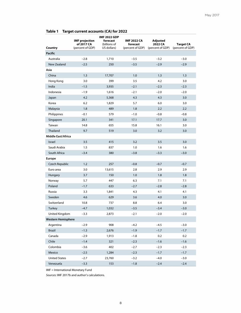
The most recent current account projections by the International Monetary Fund (IMF) in its World Economic Outlook (WEO; IMF 2017b) are the principal basis for the estimates of exchange rate changes needed to reach funda-mental equilibrium exchange rates (FEERs). Table 1 reports the Fund’s projections for 34 major economies. The first column reports the estimated current account balances for 2017, as percentages of GDP. The second column shows the projected level of GDP in 2022, the most distant year forecast.28 The third column indicates the IMF’s projection for the current account balance in 2022, based on real effec-tive exchange rates (REERs) for the month of February. The fourth column shows adjusted 2022 current account esti-mates, taking account of changes in REERs from February to April, the base month of this analysis.29 The adjusted esti-mate for the United States is developed independently (see appendix C). For other countries, the adjusted estimates also include the impact of allocating trading-partner shares of the special adjustment for the United States.30 The fifth column
28. The GDP data are in billions of dollars at 2022 then-current prices.
29. The percent change in the REER from February to April is applied to the country’s current account impact parameter (γ in the SMIM model), and one-half of the resulting change is added to the Fund’s February-based projection. In ad-dition, for Switzerland there is an adjustment reducing the estimated current account surplus by 3 percent of GDP to take account of foreign ownership of Swiss corporations (see Cline 2016a, 7).
30. The difference between the IMF forecast for the US cur-rent account in 2022 (–3.2 percent of GDP) and that of the present study (–4.0 percent) contributes an especially large amount to the calculated adjustments for Mexico (a current account change of +2.0 percent of GDP) and Canada (+1.7 percent).
8 9
May 2017
1
Number PB17-xx Month 2017
Table 1 Target current accounts (CA) for 2022
Country
IMF projection of 2017 CA
(percent of GDP)
IMF 2022 GDP forecast
(billions of US dollars)
IMF 2022 CA forecast
(percent of GDP)
Adjusted 2022 CA
(percent of GDP)Target CA
(percent of GDP)
Pacific
Australia –2.8 1,710 –3.5 –3.2 –3.0
New Zealand –2.5 250 –3.5 –2.9 –2.9
Asia
China 1.3 17,707 1.0 1.3 1.3
Hong Kong 3.0 399 3.5 4.2 3.0
India –1.5 3,935 –2.1 –2.3 –2.3
Indonesia –1.9 1,616 –2.1 –2.0 –2.0
Japan 4.2 5,368 4.3 4.3 3.0
Korea 6.2 1,829 5.7 6.0 3.0
Malaysia 1.8 489 1.8 2.2 2.2
Philippines –0.1 579 –1.0 –0.8 –0.8
Singapore 20.1 341 17.1 17.7 3.0
Taiwan 14.8 655 15.8 16.1 3.0
Thailand 9.7 519 3.0 3.2 3.0
Middle East/Africa
Israel 3.5 415 3.2 3.5 3.0
Saudi Arabia 1.5 837 1.0 1.6 1.6
South Africa –3.4 380 –3.8 –3.3 –3.0
Europe
Czech Republic 1.2 257 –0.8 –0.7 –0.7
Euro area 3.0 13,615 2.8 2.9 2.9
Hungary 3.7 150 1.0 1.8 1.8
Norway 5.7 447 6.3 7.1 7.1
Poland –1.7 633 –2.7 –2.8 –2.8
Russia 3.3 1,841 4.3 4.1 4.1
Sweden 4.6 629 3.6 4.0 3.0
Switzerland 10.8 737 8.8 6.4 3.0
Turkey –4.7 1,032 –3.5 –3.4 –3.0
United Kingdom –3.3 2,873 –2.1 –2.0 –2.0
Western Hemisphere
Argentina –2.9 908 –4.2 –4.5 –3.0
Brazil –1.3 2,676 –1.9 –1.7 –1.7
Canada –2.9 1,913 –1.8 0.2 0.2
Chile –1.4 321 –2.3 –1.6 –1.6
Colombia –3.6 402 –2.7 –2.3 –2.3
Mexico –2.5 1,284 –2.3 –1.7 –1.7
United States –2.7 23,760 –3.2 –4.0 –3.0
Venezuela –3.3 153 –1.8 –2.4 –2.4
IMF = International Monetary Fund
Sources: IMF 2017b and author’s calculations.

8 9
May 2017
of the table indicates the “target” current account balance. This target is set at no higher or lower than ±3 percent of GDP. For countries within this band, the target is simply the baseline adjusted forecast in the previous column.
The IMF’s projections show large current account surpluses of 16 to 17 percent of GDP in 2022 for the chronic high-surplus economies of Singapore and Taiwan. They also show relatively high surpluses for Korea (about 6 percent of GDP) and Japan (over 4 percent). Even after statistical adjustment, the Swiss surplus is also high at about 6 percent of GDP (fourth column). Other high surpluses include those of Hong Kong and Sweden (about 4 percent of GDP).31
Countries with prospective excessive deficits tend to be much closer to the 3 percent of GDP FEERs limit than several of those with excessive surpluses. Modestly exces-sive deficits are projected for Australia, South Africa, and Turkey, in the range of −3.2 to −3.5 percent of GDP (fourth column). The largest projected deficit is for Argentina (−4.5 percent of GDP in the adjusted estimate of the fourth column).
For the United States, the IMF has substantially increased its estimated medium-term deficit from that projected in the October WEO. At that time the Fund placed the 2021 current account at −2.7 percent of GDP (IMF 2016b). As discussed in Cline (2016b, 8) that projec-tion was puzzling as it showed a much smaller deficit than had been projected in other IMF analyses earlier in the year. The new medium term estimate of −3.2 percent of GDP (table 1, third column) is more plausible but still seems likely to understate the size of the baseline deficit.32 As shown in the fourth column of table 1, the present study projects the current account at −4.0 percent of GDP in 2022, as devel-oped in appendix C.
CHANGES NEEDED TO REACH FEERS
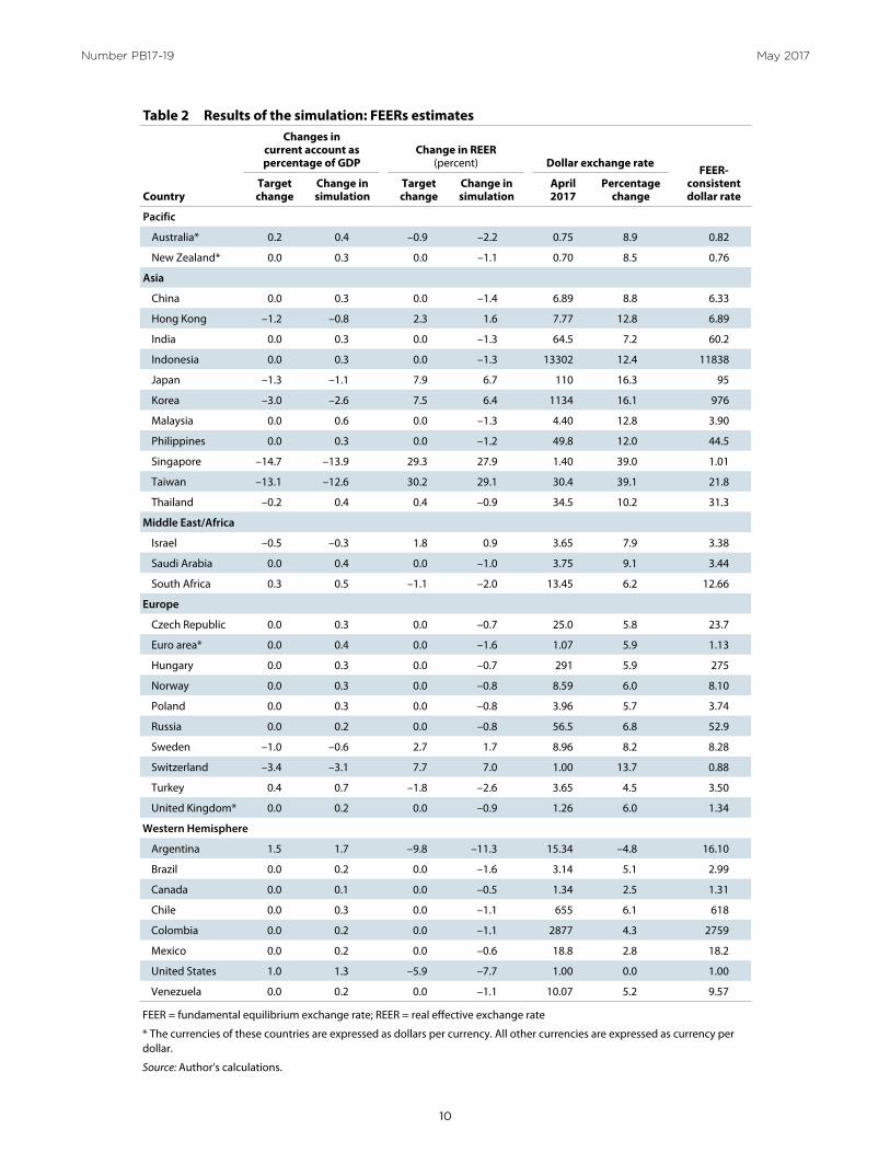
Table 2 reports the results of estimating changes in REERs and bilateral exchange rates against the dollar that approxi-mate as closely as possible the target changes in REERs in view of target changes in current accounts. The first column shows the target current account change needed to keep the
31. Oil economies Norway and Russia also have high sur-pluses (about 7 percent and 4 percent of GDP, respectively). However, the FEERs analysis does not target the current account balances of the oil economies, on grounds that high surpluses reflect the transformation of domestic resource wealth into financial assets.
32. Note further that the new WEO places the deficit at a peak of 3.65 percent of GDP in 2020. IMF 2017b.
balance within ±3 percent of GDP, based on the final two columns of table 1. The third column of table 2 indicates the percent change in the REER that would be needed to accomplish the target change in the current account. This change equals the change in current account divided by the impact parameter γ in the SMIM model. The best overall approximations of changes are then shown in the second column of table 2 for the change in the current account and the fourth column for the change in REER.
The most important needed changes in REERs in the simulation results are the reduction in the level of the dollar by about 8 percent, the real appreciations of 6 to 7 percent needed for the Japanese yen and Korean won, and the real appreciations by 28 to 29 percent needed for Singapore and Taiwan to curb high current account surpluses. Other notable changes needed include real effective depreciation of 11 percent for Argentina, and an appreciation in the REER by 7 percent for Switzerland.
Significant cases where misalignment has widened from the November estimates (Cline 2016b) include the cases of Japan (with undervaluation increasing from about 3 to about 7 percent) and Argentina (with overvaluation rising from 7 to 11 percent). Significant cases where misalign-ments have moderated include Australia and New Zealand (with overvaluation narrowing from 4 to 6 percent to 1 to 2 percent) and especially Turkey (overvaluation falling from 9 to about 3 percent).33
In the key case of the United States, the estimated misalignment has remained almost unchanged from October, with calculated overvaluation still at about 8 percent. This finding reflects the reversal by April of most of the run-up in the dollar following the 2016 presidential election.34 The new result also reflects a return in the estimate of the current account impact parameter to its previous level, somewhat higher than used in the November estimates (see appendix C).
Because of the overvaluation of the dollar, the FEER estimates for most currencies show a significant apprecia-tion against the dollar, as shown in the next-to-last column of table 2. Figure 3 summarizes changes in exchange rates needed to reach FEERs, both in terms of change in the REER and change in the bilateral rate against the dollar, arrayed from largest needed appreciations at the left to the largest needed depreciations at the right.
33. The change in Turkey reflects a nominal depreciation of about 16 percent against the US dollar from October to April.
34. The broad real index of the dollar rose from 99.0 in October to a peak of 102.8 in December but fell back to 99.8 in April. Federal Reserve 2017a.
10 11
Number PB17-19 May 2017
2 3
Number PB17-xx Month 2017
Table 2 Results of the simulation: FEERs estimates
Country
Changes in current account as percentage of GDP
Change in REER (percent) Dollar exchange rate
FEER-consistent dollar rate
Target change
Change in simulation
Target change
Change in simulation
April 2017
Percentage change
Pacific
Australia* 0.2 0.4 –0.9 –2.2 0.75 8.9 0.82
New Zealand* 0.0 0.3 0.0 –1.1 0.70 8.5 0.76
Asia
China 0.0 0.3 0.0 –1.4 6.89 8.8 6.33
Hong Kong –1.2 –0.8 2.3 1.6 7.77 12.8 6.89
India 0.0 0.3 0.0 –1.3 64.5 7.2 60.2
Indonesia 0.0 0.3 0.0 –1.3 13302 12.4 11838
Japan –1.3 –1.1 7.9 6.7 110 16.3 95
Korea –3.0 –2.6 7.5 6.4 1134 16.1 976
Malaysia 0.0 0.6 0.0 –1.3 4.40 12.8 3.90
Philippines 0.0 0.3 0.0 –1.2 49.8 12.0 44.5
Singapore –14.7 –13.9 29.3 27.9 1.40 39.0 1.01
Taiwan –13.1 –12.6 30.2 29.1 30.4 39.1 21.8
Thailand –0.2 0.4 0.4 –0.9 34.5 10.2 31.3
Middle East/Africa
Israel –0.5 –0.3 1.8 0.9 3.65 7.9 3.38
Saudi Arabia 0.0 0.4 0.0 –1.0 3.75 9.1 3.44
South Africa 0.3 0.5 –1.1 –2.0 13.45 6.2 12.66
Europe
Czech Republic 0.0 0.3 0.0 –0.7 25.0 5.8 23.7
Euro area* 0.0 0.4 0.0 –1.6 1.07 5.9 1.13
Hungary 0.0 0.3 0.0 –0.7 291 5.9 275
Norway 0.0 0.3 0.0 –0.8 8.59 6.0 8.10
Poland 0.0 0.3 0.0 –0.8 3.96 5.7 3.74
Russia 0.0 0.2 0.0 –0.8 56.5 6.8 52.9
Sweden –1.0 –0.6 2.7 1.7 8.96 8.2 8.28
Switzerland –3.4 –3.1 7.7 7.0 1.00 13.7 0.88
Turkey 0.4 0.7 –1.8 –2.6 3.65 4.5 3.50
United Kingdom* 0.0 0.2 0.0 –0.9 1.26 6.0 1.34
Western Hemisphere
Argentina 1.5 1.7 –9.8 –11.3 15.34 –4.8 16.10
Brazil 0.0 0.2 0.0 –1.6 3.14 5.1 2.99
Canada 0.0 0.1 0.0 –0.5 1.34 2.5 1.31
Chile 0.0 0.3 0.0 –1.1 655 6.1 618
Colombia 0.0 0.2 0.0 –1.1 2877 4.3 2759
Mexico 0.0 0.2 0.0 –0.6 18.8 2.8 18.2
United States 1.0 1.3 –5.9 –7.7 1.00 0.0 1.00
Venezuela 0.0 0.2 0.0 –1.1 10.07 5.2 9.57
FEER = fundamental equilibrium exchange rate; REER = real effective exchange rate
* The currencies of these countries are expressed as dollars per currency. All other currencies are expressed as currency per dollar.
Source: Author’s calculations.

10 11
May 2017
–20
–1001020304050
TAI
SGP
SWZ
KOR
JPN
HK
SWE
ISR
CAN
MEX
HU
NCZ
HPO
LU
KTH
ACO
LN
ZCH
LPH
LID
NIN
DM
LSCH
NBR
ZEU
RSA
FA
US
TUR
US
ARG
Chan
ge in
REE
R (p
erce
nt)
Chan
ge in
dol
lar r
ate
(per
cent
)
perc
ent
Figu
re 3
C
hang
es n
eede
d to
reac
h FE
ERs
ARG
= A
rgen
tina,
AU
S =
Aus
tral
ia, B
RZ =
Bra
zil,
CAN
= C
anad
a, C
HL
= Ch
ile, C
HN
= C
hina
, CO
L =
Colo
mbi
a, C
ZH =
Cze
ch R
epub
lic, E
UR
= Eu
ro a
rea,
HK
= H
ong
Kong
, H
UN
= H
unga
ry, I
ND
= In
dia,
IDN
= In
done
sia,
ISR
= Is
rael
, JPN
= Ja
pan,
KO
R =
Kore
a, M
LS =
Mal
aysi
a, M
EX =
Mex
ico,
NZ
= N
ew Z
eala
nd, P
HL
= Ph
ilipp
ines
, PO
L =
Pola
nd, S
GP
= Si
ngap
ore,
SA
F =
Sout
h A
fric
a, S
WE
= Sw
eden
, SW
Z =
Switz
erla
nd, T
AI =
Tai
wan
, TH
A =
Tha
iland
, TU
R =
Turk
ey, U
K =
Uni
ted
King
dom
, U
S =
Uni
ted
Stat
esFE
ER =
fund
amen
tal e
quili
briu
m e
xcha
nge
rate
; REE
R =
real
e�e
ctiv
e ex
chan
ge ra
te
Sour
ce: A
utho
r’s c
alcu
latio
ns.

12 13
May 2017
CONCLUSION
The US dollar remains overvalued by about 8 percent. There is considerable risk that the dollar will rise further and the overvaluation will increase. Already with the current market-expected differential in long-term interest rates by 2018, past currency relationships would predict a rise in the dollar by 3 to 5 percent against the euro and 4 to 15 percent against the yen. Rising interest differentials currently associated with unsynchronized timetables for normalizing monetary policy in the United States, the euro area, and Japan could be exacerbated by a move toward major US fiscal stimulus. The tax reform plan outlined by the Trump administration at the end of April could cause such a stimulus, considering that it would cut revenues by about 2 percent of GDP. Even achievement of the steady
3 percent growth envisioned by the tax proposal authors would be unlikely to recover more than about one-third to one-half of the direct revenue loss. Yet 3 percent growth would be difficult to achieve given the slow labor expansion associated with demographics and realistic limits to accel-eration of productivity growth. If fiscal reform adopted the border tax adjustment proposed by House Republicans, the deficits might be somewhat smaller, but there could be a sizable exchange market shock strengthening the dollar—albeit likely by considerably less than assumed in the theory border tax advocates cite. Even though there has been encouraging moderation in the Trump administra-tion’s confrontational trade policy approach, trade conflict could escalate if the dollar were to rise considerably further because of these forces.
© Peterson Institute for International Economics. All rights reserved. This publication has been subjected to a prepublication peer review intended to ensure analytical quality.
The views expressed are those of the author. This publication is part of the overall program of the Peterson Institute for International Economics, as endorsed by its Board of Directors, but it does not neces-
sarily reflect the views of individual members of the Board or of the Institute’s staff or management. The Peterson Institute for International Economics is a private nonpartisan, nonprofit institution for rigorous,
intellectually open, and indepth study and discussion of international economic policy. Its purpose is to identify and analyze important issues to make globalization beneficial and sustainable for the people of the United States and the world, and then to develop and communicate practical new approaches for dealing with them. Its work is funded by a highly diverse group of
philanthropic foundations, private corporations, and interested individuals, as well as income on its capital fund. About 35 percent of the Institute’s resources in its latest fiscal year were provided by contributors from outside the United States.
A list of all financial supporters is posted at https://piie.com/sites/default/files/supporters.pdf.

12 13
May 2017
APPENDIX A
TRENDS IN MAJOR CURRENCIES SINCE THE GREAT RECESSION
Nearly ten years ago the first financial tremors of the Great Recession emerged, with the closure of two mortgage-backed securities (MBS) funds by Bear Stearns (in July 2007) and soon afterwards the suspension by BNP Paribas of withdrawals from three investment funds because of MBS liquidity problems (Cline 2010, 273). It is useful to review the path of the real exchange rates for the five most important currencies over the decade that followed.35
With the average for 2007 as an index base of 100, for the first two months of 2017 the real effective exchange rate (REER) stood at an average index of 112.1 for the dollar, 84.1 for the euro, 138.0 for the renminbi, 92.6 for the yen, and 76.2 for the pound.36 The dollar has recently been at its strongest level in the last decade, although at its highest recent point (December 2016) it remained 20 percent below its Reagan-era peak (March 1985) and 9 percent below its more recent high point (February 2002).37 The dollar had eased through most of 2008 but then surged from a safe-haven effect at the height of the financial crisis. In late 2010 the second round of quantitative easing (QE2) spurred a decline in the dollar to a more moderate plateau that lasted through mid-2014 (and initially prompted charges of “currency wars;” see Cline and Williamson 2010). The major upswing in the dollar since mid-2014 has been driven by the sharp fall in oil and commodity prices and the asynchronous timing of monetary policy phases, with the US ending quantitative easing but the euro area and Japan pursuing it.
35. The five currencies shown in figure 1 are the only currencies included in the IMF’s special drawing right (SDR). Their weights in the SDR are: US dollar, 41.73 percent; euro, 30.93 percent; Chinese renminbi, 10.92 percent; Japanese yen, 8.33 percent; and pound sterling, 8.09 percent. IMF 2016a.
36. Using the broad real effective exchange rate index of the BIS (2017), deflating by consumer prices.
37. Using the broad real effective exchange rate index of the Federal Reserve (2017a).
Figure A.1 Real e�ective exchange rates, 2007–17: US dollar, euro, Chinese renminbi, Japanese yen, and pound sterling
Source: BIS 2017.
70
80
90
100
110
120
130
140
150
2007 2008 2009 2010 2011 2012 2013 2014 2015 2016 2017
ChinaEuro areaJapanUnited KingdomUnited States
index (2007 = 100)

14 15
May 2017
The Chinese renminbi has shown the most persistent real appreciation. It was pulled up early in the financial crisis by its tie to the dollar. Its long-term appreciation reflects the Balassa-Samuelson effect of rising relative productivity in the trad-able sector of a rapidly growing emerging-market economy. The pause and then partial reversal of this trend beginning in 2015 reflects widening capital outflows associated with China’s move to a more market-determined exchange rate and looser capital controls (in part prompted by its pursuit of inclusion of the renminbi in the SDR), combined with a shift away from expectations of persistent appreciation. Since mid-2014 external reserves have fallen from $4.01 trillion to $3.02 trillion as the authorities have drawn down reserves to keep the renminbi from falling, whereas previously China had built up large reserves by intervening to curb appreciation.38
The path of the euro over the past decade shows two downward steps to lower plateaus. The first significant decline occurred in 2010, the year when sovereign debt crises struck Greece, Ireland, and Portugal. The second step down occurred in 2015, the first year of quantitative easing by the European Central Bank. Japan’s real exchange rate has been marked by a high plateau in 2009 through 2012, followed by a sharply lower plateau in 2013 through early 2017. The decline of about 25 percent from the first period to the second was driven by the economic program of the new prime minister Shinzo Abe’s government, which pledged to boost inflation to 2 percent and to pursue aggressive quantitative easing that would double the monetary base over two years (Cline 2013, 2). For the United Kingdom, the real exchange rate fell sharply in the Great Recession and remained at a relatively low plateau during 2009–13. The decline by about 25 percent from 2007 to the end of 2008 reflected concern about large government deficits and vulnerability to banking crisis. Even so, it was considered by some to be “… an overdue adjustment after a long period in which sterling was overpriced.”39 During 2014–15 the pound regained much of the loss, but the shock of Brexit then brought the currency back to its Great Recession lows.
38. Neely (2016) suggests that 60 percent of reserves are in dollars. If the other three reserve currencies in the SDR are con-sidered representative of nondollar reserves, and if their proportionate changes against the dollar in this period are considered (−21.5 percent for the euro, −10.8 percent for the yen, and −26.2 percent for the pound), the weighted average decline of nondollar assets (using SDR weights) would have contributed an 8 percent decline in reported reserves from valuation effects, or about one-third of the total decline.
39. “Fall from grace,” Economist, December 18, 2008.

14 15
May 2017
APPENDIX B
EXCHANGE RATE EFFECTS OF A PROPOSED BORDER TAX ADJUSTMENT
As highlighted in the main text, a new consideration for the US dollar is that a major corporate tax reform proposed by Republicans in the House of Representatives would in effect impose a border tax adjustment (BTA) of 20 percent on all imports and grant complete exemption of exports. Supporters of the proposal argue that the tax would raise about $100 billion annually (being in effect a 20 percent tax on the annual deficit in goods trade of about $500 billion), but that it would leave importers held harmless because the induced appreciation of the dollar would fully offset the tax. The same argument is used as a justification for why the measure would not be protectionist, on grounds that the exchange rate move would neutralize any extra incentive to exports and disincentive to imports.
HOW MUCH IS THE DOLLAR SUPPOSED TO APPRECIATE?
The destination-based cash flow tax (DBCFT) in the Ryan-Brady proposal would place a 20 percent tax on a base that exempts exports but does not permit deduction of imports (Cline 2017). A reasonable, intuitive interpretation would be that the effect would be equivalent to a new tariff of 20 percent on all imports. If consumers were to be held harmless, as argued by supporters of the proposal, by implication the dollar would need to rise by 20 percent so that the payment in tax revenue would be exactly offset by the decline in the dollar cost of the same foreign currency value of imports.40
Because the tax is levied through eliminating the deductibility of imports in the corporate tax base, however, it turns out that the expected appreciation would be 25 percent.41 Thus, suppose the corporate revenue remains unchanged at R, consistent with no change in cost to consumers. Suppose the firm has domestic labor and input costs of Cd, and has imported component goods costing M$. Defining π as after-tax profit and τ as the tax rate (20 percent in the DBCFT), under existing treatment, allowing deductibility of imports after-tax profits would be:
1
(B.1)
If import costs can no longer be deducted, then after-tax profits become:
1
(B.2)
If after-tax profits are to remain unchanged, equation B.2 equals equation B.1. Eliminating their common element gives:
1
(B.3)
The dollar value of imports equals the foreign currency value of imports, assumed to be unchanged at MF, divided by the exchange rate expressed as foreign currency units per dollar, E.
Thus:
1
(B.4)
Cancelling and rearranging,
1
(B.5)
With τ= 0.2, the new exchange rate will be 1.25 times the original rate of foreign currency per dollar, a 25 percent appreciation.
40. At the original exchange rate, imports that previously cost $100 would cost $120, including the tax. If the dollar rose by 20 percent, the foreign currency cost of the import would fall to $83.33 (=100FC/(1.2FC/$), where FC = foreign currency). Imposition of the 20 percent tax would return the import cost to $100 (=$83.33 x 1.2).
41. Auerbach (2017) states that the appreciation would be 25 percent.

16 17
May 2017
WHAT IS THE EVIDENCE SO FAR?
After three months of considerable publicity for the BTA, however, financial markets have not shown the response that might have been expected if the dollar-boosting impact were fully credible. If the perceived probability of a 20 percent BTA had risen from zero to, say, 50 percent, and if currency market participants fully believed in a prompt and full dollar response to the BTA, then the dollar should have risen by 12.5 percent. Instead, from the end of 2016 to March 31, 2017, a simple average index of the dollar against the euro and the yen fell by 1.2 percent. Similarly, from December to March the monthly average of the Federal Reserve’s broad real exchange rate index fell from 102.84 to 101.22 (Federal Reserve 2017a), or by 1.6 percent.
Figure B.1 shows two possible indicators of the perceived probability of a BTA. The first is a daily count of financial press articles that mention the border adjustment tax.42 After remaining in low single digits in most of December and the first half of January, the number of such articles jumped to about 40 on January 17, following an interview in which President Trump called the BTA“too complicated.” The count surged to 80 on January 27, the day after the president mentioned a “big border tax” against Mexico as well as a specific figure of 20 percent. Another surge brought the count slightly above 100 on March 1, following the president’s measured speech to Congress and its tone implying cooperation with Republican plans (even though the speech did not mention the BTA specifically). The news count then fell to a modest plateau, before rising briefly to about 70 on March 27, the first business day after collapse of the healthcare bill. The subject of the BTA likely resurfaced then because of the expectation of a shift to tax reform as the legislative priority.
42. The news count index is from Bloomberg. The figure reports the index response to the queries “border adjustment tax” and “border tax adjustment.” The responses included articles from 25 leading financial press entities.
Figure B.1 News article count and stock price indicators of attention to border tax adjustment
Note: The export/import stock price ratio is the simple average for the export-stock indexes to the simple average for the import-stock indexes.Sources: Bloomberg and author’s calculations.
0.95
0.97
0.99
1.01
1.03
1.05
1.07
1.09
1.11
1.13
1.15
0
20
40
60
80
100
120
ArticlesExport/import stock price
number of articles export/import stock price ratio
Decem
ber 1, 2
016
Decem
ber 8, 2
016
Decem
ber 15, 2
016
Decem
ber 22, 2
016
Decem
ber 29, 2
016Ja
nuary 5, 2
017Ja
nuary 12, 2
017Ja
nuary 19, 2
017Ja
nuary 26, 2
017Feb
ruary
2, 2017
Febru
ary 9, 2
017
Febru
ary 16, 2
017
Febru
ary 23, 2
017March
2, 2017
March 9, 2
017March
16, 2017
March 23, 2
017March
30, 2017

16 17
May 2017
The second indicator in figure B.1 compares the path of stock prices for six export-oriented firms prominent in supporting the BTA, relative to stock prices for seven import-oriented firms prominent in opposing it.43 Because the BTA applies a 20 percent tax to imports but exempts exports, it should favor export firms relative to import firms unless induced offsetting exchange rate effects are prompt and complete. The ratio does indeed show a meaningful relative gain for export firms, by about 10 percent for the four months ending March 31. Moreover, the two episodes of movement in the “wrong” direction when compared to the news count were indeed days in which the news was active but the tone unfavorable (“too complicated” for January 17; commentary that the BTA could be too controversial, for March 2744).
Figure B.2 repeats the relative stock price indicator and compares it to the path of the bilateral exchange rates of the dollar against the euro and yen, once again with indexes set at 100 for December 1, 2016. From the beginning of December to the end of March, the dollar fell 1.2 percent against a simple average index for the two currencies. From the dollar’s strongest point in this period, on December 16, to its weakest point, March 27, the dollar’s corresponding decline against the two currencies was 5 percent.45
In summary, so far the market evidence on exchange rate expectations regarding the BTA is at best ambiguous and arguably goes in the wrong direction for the theoretical impact invoked by supporters. The dollar has tended to fall rather than rise as attention has become focused on the BTA. Moreover, stock prices of export firms relative to those of import
43. The export firms are: Boeing, Caterpillar, Dow Chemical, Oracle, and Pfizer; the import firms are Walmart, Target, Nike, Best Buy, Gap, Tesoro, and Toyota. Each stock price is set at an index of 100 for December 1, 2016. The stock price ratio in the figure is the ratio of the simple average for the export-stock indexes to the simple average for the import-stock indexes.
44. For the latter, a typical article cited one bank advisory view stating that “The border adjustment tax, the most controversial piece of current tax-reform discussions, is less likely to pass.” Andrew Ross Sorkin, New York Times, March 27, 2017.
45. The figure also changes the BTA stock indicator terminology to “likelihood,” as the ambiguity of negative as well as posi-tive news in news-count of figure 1 is no longer present.
0.85
0.90
0.95
1.00
1.05
1.10
1.15
1.20
85
90
95
100
105
110
115
120
Yen/dollarEuro/dollarExport/import stock price
index (2007 = 100) export/import stock price ratio
Figure B.2 Strength of the dollar against the euro and yen (left), and stock price indicator of border tax adjustment likelihood (right)
Note: The export/import stock price ratio is the simple average for the export-stock indexes to the simple average for the import-stock indexes.Sources: Bloomberg and author’s calculations.
Decem
ber 1, 2
016
Decem
ber 8, 2
016
Decem
ber 15, 2
016
Decem
ber 22, 2
016
Decem
ber 29, 2
016Ja
nuary 5, 2
017Ja
nuary 12, 2
017Ja
nuary 19, 2
017Ja
nuary 26, 2
017Feb
ruary
2, 2017
Febru
ary 9, 2
017
Febru
ary 16, 2
017
Febru
ary 23, 2
017March
2, 2017
March 9, 2
017March
16, 2017
March 23, 2
017March
30, 2017
18 19
May 2017
firms have tended to rise, pointing toward greater influence of the view that imports would be discouraged by the BTA and exports encouraged, rather than the view that there would be no relative impact thanks to the fully offsetting appreciation of the dollar.
HOW MUCH DOES THE DOLLAR RESPOND TO CHANGES IN THE TRADE BALANCE?
These patterns might surprise many economists, if the financial press is to believed. A typical article suggests that most economists think the dollar would fully appreciate to offset the BTA.46 Prominent examples include Martin Feldstein and Paul Krugman.47 A notable exception is Buiter (2017), who argues that the exchange rate could go either way, depending on the nature of export and import firms’ pricing-to-market behavior.
Long-time exchange rate practitioners might well question the putative view of economists that there would be a prompt and full exchange rate offset of the BTA.48 There have been long periods when a rising trade deficit did not trigger a deprecia-tion of the dollar. Yet the exchange rate effect argued by advocates of the DBCFT is essentially a fluid mechanics mechanism whereby the height of liquid in the dollar-strength pipe depends directly on the flow volume of euro, yen, and other foreign currency inflows from trade compared to that of dollar outflows from trade. The slightest cutback of imports caused by a 20 percent tariff, in this framework, causes more euros and yen from foreign exporters to chase fewer dollars from US importers, requiring the dollar to rise until the initial trade flows are restored.
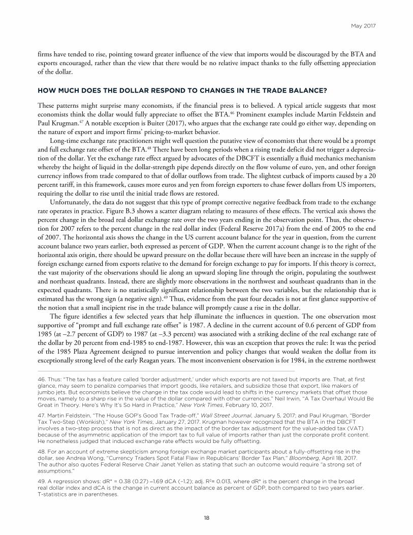
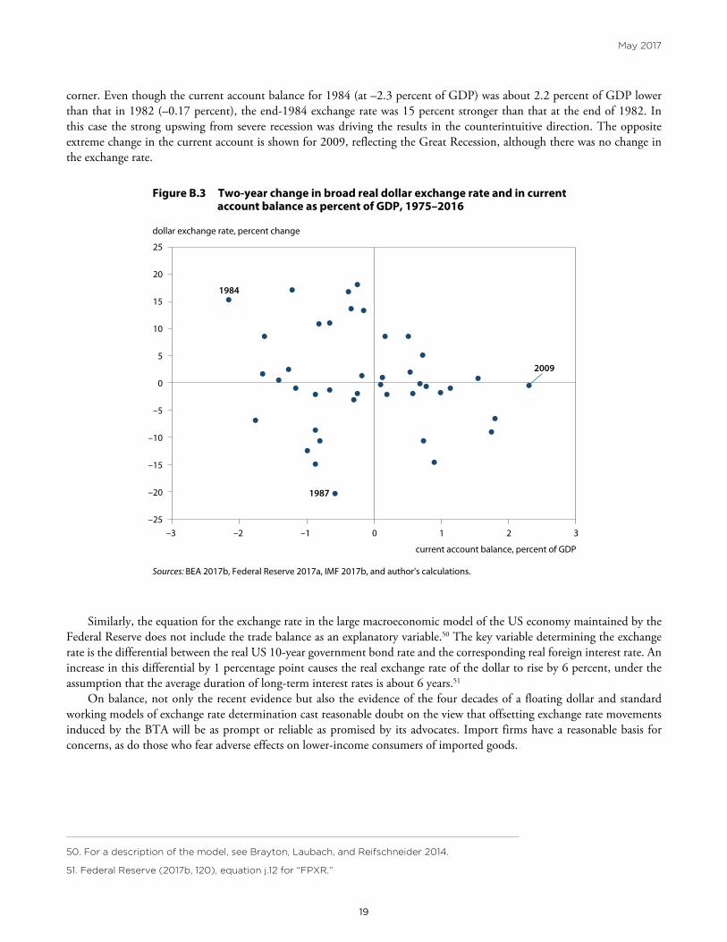
Unfortunately, the data do not suggest that this type of prompt corrective negative feedback from trade to the exchange rate operates in practice. Figure B.3 shows a scatter diagram relating to measures of these effects. The vertical axis shows the percent change in the broad real dollar exchange rate over the two years ending in the observation point. Thus, the observa-tion for 2007 refers to the percent change in the real dollar index (Federal Reserve 2017a) from the end of 2005 to the end of 2007. The horizontal axis shows the change in the US current account balance for the year in question, from the current account balance two years earlier, both expressed as percent of GDP. When the current account change is to the right of the horizontal axis origin, there should be upward pressure on the dollar because there will have been an increase in the supply of foreign exchange earned from exports relative to the demand for foreign exchange to pay for imports. If this theory is correct, the vast majority of the observations should lie along an upward sloping line through the origin, populating the southwest and northeast quadrants. Instead, there are slightly more observations in the northwest and southeast quadrants than in the expected quadrants. There is no statistically significant relationship between the two variables, but the relationship that is estimated has the wrong sign (a negative sign).49 Thus, evidence from the past four decades is not at first glance supportive of the notion that a small incipient rise in the trade balance will promptly cause a rise in the dollar.
The figure identifies a few selected years that help illuminate the influences in question. The one observation most supportive of “prompt and full exchange rate offset” is 1987. A decline in the current account of 0.6 percent of GDP from 1985 (at –2.7 percent of GDP) to 1987 (at –3.3 percent) was associated with a striking decline of the real exchange rate of the dollar by 20 percent from end-1985 to end-1987. However, this was an exception that proves the rule: It was the period of the 1985 Plaza Agreement designed to pursue intervention and policy changes that would weaken the dollar from its exceptionally strong level of the early Reagan years. The most inconvenient observation is for 1984, in the extreme northwest
46. Thus: “The tax has a feature called ‘border adjustment,’ under which exports are not taxed but imports are. That, at first glance, may seem to penalize companies that import goods, like retailers, and subsidize those that export, like makers of jumbo jets. But economists believe the change in the tax code would lead to shifts in the currency markets that offset those moves, namely to a sharp rise in the value of the dollar compared with other currencies.” Neil Irwin, “A Tax Overhaul Would Be Great in Theory. Here’s Why It’s So Hard in Practice,” New York Times, February 10, 2017.
47. Martin Feldstein, “The House GOP’s Good Tax Trade-off,” Wall Street Journal, January 5, 2017; and Paul Krugman, “Border Tax Two-Step (Wonkish),” New York Times, January 27, 2017. Krugman however recognized that the BTA in the DBCFT involves a two-step process that is not as direct as the impact of the border tax adjustment for the value-added tax (VAT) because of the asymmetric application of the import tax to full value of imports rather than just the corporate profit content. He nonetheless judged that induced exchange rate effects would be fully offsetting.
48. For an account of extreme skepticism among foreign exchange market participants about a fully-offsetting rise in the dollar, see Andrea Wong, “Currency Traders Spot Fatal Flaw in Republicans’ Border Tax Plan,” Bloomberg, April 18, 2017. The author also quotes Federal Reserve Chair Janet Yellen as stating that such an outcome would require “a strong set of assumptions.”
49. A regression shows: dR* = 0.38 (0.27) −1.69 dCA (–1.2); adj. R2= 0.013, where dR* is the percent change in the broad real dollar index and dCA is the change in current account balance as percent of GDP, both compared to two years earlier. T-statistics are in parentheses.
18 19
May 2017
corner. Even though the current account balance for 1984 (at –2.3 percent of GDP) was about 2.2 percent of GDP lower than that in 1982 (–0.17 percent), the end-1984 exchange rate was 15 percent stronger than that at the end of 1982. In this case the strong upswing from severe recession was driving the results in the counterintuitive direction. The opposite extreme change in the current account is shown for 2009, reflecting the Great Recession, although there was no change in the exchange rate.
Similarly, the equation for the exchange rate in the large macroeconomic model of the US economy maintained by the Federal Reserve does not include the trade balance as an explanatory variable.50 The key variable determining the exchange rate is the differential between the real US 10-year government bond rate and the corresponding real foreign interest rate. An increase in this differential by 1 percentage point causes the real exchange rate of the dollar to rise by 6 percent, under the assumption that the average duration of long-term interest rates is about 6 years.51
On balance, not only the recent evidence but also the evidence of the four decades of a floating dollar and standard working models of exchange rate determination cast reasonable doubt on the view that offsetting exchange rate movements induced by the BTA will be as prompt or reliable as promised by its advocates. Import firms have a reasonable basis for concerns, as do those who fear adverse effects on lower-income consumers of imported goods.
50. For a description of the model, see Brayton, Laubach, and Reifschneider 2014.
51. Federal Reserve (2017b, 120), equation j.12 for “FPXR.”
Figure B.3 Two-year change in broad real dollar exchange rate and in current account balance as percent of GDP, 1975–2016
Sources: BEA 2017b, Federal Reserve 2017a, IMF 2017b, and author’s calculations.
1984
1987
2009
–25
–20
–15
–10
–5
0
5
10
15
20
25
–3 –2 –1 0 1 2 3
dollar exchange rate, percent change
current account balance, percent of GDP

20 21
May 2017
THE I-S IDENTITY, THE INTEREST RATE, AND INDUCED EXCHANGE RATE CHANGE
One reason the induced exchange rate offset is not prompt and reliable is that financial factors such as interest rate differ-entials can swamp trade effects, considering that daily foreign exchange trading volumes far exceed magnitudes related to currency needed for trade (as emphasized by Posen 2017).52 Another reason is that whereas many economists focus solely on the national accounts identity for the trade balance (equal to the excess of saving over investment) and implicitly treat it as binding and exogenous, the external accounts instead involve two simultaneous equations that must both hold. The second of these equations is a price-activity equation involving activity levels and price (exchange rate) levels that determine import and export flows. There is no reason to treat the price-activity equation as strictly endogenous and the I-S equation as strictly exogenous (Cline 1994; 2017). The two equations essentially correspond to the two traditional alternative approaches to the trade balance: the “absorption” approach (I−S identity) and the “elasticities” approach (whereby imports and exports respond to price signals from the exchange rate and to activity levels; Cline 2005, 136). Inclusion of the elasticities approach means that a 20 percent tax on imports might really curb imports, and a 20 percent preferential treatment of exports versus domestic sales might really expand exports. Changes could occur in some of the components of the I−S identity, such that there might not be a fully offsetting exchange rate movement that leaves the trade balance unchanged.
If the economy is at full employment, the rise in exports and import substitutes will boost output demand, tending to raise interest rates and in turn curb investment and interest-sensitive consumption. In 2016, goods exports amounted to 7.9 percent of US GDP, and goods imports, 11.9 percent (BEA 2017a). Assuming the price elasticity is unity, the 20 percent BTA would boost exports by 1.58 percent of GDP and reduce imports by 2.38 percent of GDP.53 If two-thirds of the cutback in imports translated to increased production of domestic import substitutes, and the other one-third simply reduced consumption, the consequence would be a boost to output demand by 1.58 percent on the import side as well. The total increase in output by 3.16 percent of GDP above potential output would induce an increase in the interest rate by 0.5 x 3.16 percent = 1.58 percent if the Taylor (1993) rule were followed. Based on US experience in 1990–2007, the median annual change in the 10-year interest rate is the fraction 0.4 of the annual change in the policy interest rate.54 So the change in the long-term rate would amount to 0.4 x 1.58 = 0.63 percent.
For the euro and the yen, in the model estimates in the main text (across both the level and first-difference results), the average impact of a 100 basis-point increase in the US long-term interest differential is to boost the dollar by 11.1 percent. This impact would imply an increase in the dollar by 7 percent (11.1 x 0.63) as the consequence of the BTA. If instead one applies the Federal Reserve’s macroeconomic model (FRB/US) coefficient of 6 percent increase in the dollar from a 100 basis-point increase in the long-term interest differential, the dollar’s rise induced by the BTA would amount to 3.8 percent initially, and some additional rise over time from the buildup in net foreign assets.55 These illustrative calculations suggest that at least in the initial years of the DBCFT, the size of the induced dollar appreciation would be well below the 25 percent expected by its advocates, perhaps well below half this amount, especially in the early years.
LONGER TERM EFFECTS; PROTECTION ISSUES
Returning to the lack of evidence of near-term market exchange rate response to increased trade balances suggested by figure B.3, one response of supporters of the full exchange rate offset argument might reasonably be that “in the long run” the rela-tive supply and demand of foreign exchange would tend to bring about the full offset. In this view, there is too much noise
52. Thus, in 2016 daily turnover in global foreign exchange trading amounted to an average of $5.1 trillion, or 40 times the amount needed for current account transactions. Moore, Schrimpf, and Sushko 2016, 36.
53. For simplicity, this calculation treats the impact as equivalent to that of a 20 percent import tariff and 20 percent export subsidy.
54. Calculated from Bloomberg data on the 10-year government bond rate and the discount rate.
55. The FRB/US equation indicates that a 10 percent rise of GDP in net foreign assets would boost the dollar by 2 percent. This country-risk parameter appears exaggerated. Thus, US net foreign assets have fallen by 30 percent of GDP over the past decade (see table C.1 below), but it would be difficult to argue that the dollar is 6 percent lower than it would have been in the absence of this change. With a posited 3 percent of GDP increase in the trade balance from the BTA, the cumulative effect over a decade would be an increase in net foreign assets on the order of 30 percent of GDP. (Lower dollar translation of for-eign equity assets would tend to curb the extent of the increase.) The country-risk parameter in the FRB/US model would ac-cordingly imply an increase of 6 percent in the dollar, bringing the total increase by the end of the decade to about 10 percent (including the initial boost from the interest rate differential effect).

20 21
May 2017
in even two-year horizons to warrant the doubts about the assumed effects. A practical problem with this interpretation is a potential time inconsistency in the DBCFT-BTA approach. The approach assumes that the United States is alone in shifting its corporate tax system. Instead, over a horizon of say a decade, it would be far more likely that other countries would also adopt the DBCFT to replace their corporate tax regimes, not in defiant retaliation but rather in the spirit of imitating a better mousetrap. But then by definition it would be impossible for the real dollar to rise, because all other currencies would experience the same incipient upward pressure.
Finally, the DBCFT and its BTA pose the problem of being protectionist, because the regime does not give like treat-ment to imports and domestic goods. Domestic sales can deduct labor and other input costs in determining the tax base, whereas the full value of imports is subject to the tax. The response of the advocates of the DBCFT is that the exchange rate appreciation will completely offset any distortion of incentives resulting from this asymmetric treatment, but so long as the exchange rate adjusts in a delayed and incomplete fashion, the protection persists even within this framework. I have observed that the protectionist nature of the regime might reasonably be corrected by allowing a standard deduction of, say, 70 percent of import value from the taxable base to represent labor and input costs.56 But such an approach would mean much less revenue from the proposal and hence less scope for it to finance other tax cuts in the reform agenda.
56. “Protectionism in the Guise of Tax Reform,” Letter to the editor, New York Times, March 13, 2017.

22 23
May 2017
APPENDIX C
US CURRENT ACCOUNT OUTLOOK
For nonoil goods and services, the projections of this study apply the model described in Cline (2016b), with a slight updating of parameters.57 The appreciation of the REER for the dollar by about 17 percent from its average level in 2014 causes a substantial widening in the nonoil trade balance after a two-year lag.
For oil and gas, the projections are based on EIA (2017a) projections of imports and exports in overall US energy supply. Imports of crude oil and petroleum liquid products are expected to ease from 21.96 quads58 in 2017 to 20.8 quads in 2022, whereas petroleum exports are projected to rise from 10.5 quads to 13.22 quads. The price of Brent oil is projected to rise from $43.43 in 2016 to about $51 in 2017, $75 by 2019, and $92 in 2022. After converting to equivalent million barrels of oil and harmonizing with actual oil trade values in 2013–16, the resulting projections show the value of oil imports increasing modestly from an average of 0.95 percent of GDP in 2017 to 1.32 percent by 2022, and the value of exports rising more substantially from 0.53 percent of GDP in 2017 to 0.98 percent by 2022.59 From 2017 to 2022, the physical volume of imports declines by about 5 percent, whereas that of exports rises by about 26 percent, and the oil price rises by 80 percent. The overall effect is that net oil trade stays at a plateau of about −0.35 percent of GDP in 2017 through 2022 after having narrowed sharply from about −2 of GDP in 2006.60
The projection for capital services continues to show the anomaly whereby there is a sizable surplus on capital services (net income) despite a large and growing net international liability position. This phenomenon reflects a persistent large gap between earnings on US direct investment abroad (averaging 7.9 percent annually in 2006–16) and earnings on foreign
57. The model (corresponding to equation A5 in Cline 2016b), estimated for 1990–2016, is: NOTBt = 14.429 −0.114 R*t-2 −3.957 QU/QRt −0.103 gdift −0.113 T, where NOTB is the balance on nonoil goods and services as a percent of GDP, R*is the real effec-tive exchange rate, QU/QR is the ratio of real US GDP to real GDP of the rest of the world at market exchange rates (with 1990 as the base), gdif is the excess of US growth over rest-of-world growth for the year in question, and T is a time variable.
58. Quadrillion British Thermal Units.
59. One quad is equivalent to 180.2 million barrels of oil. Estimates of million barrels based on quads of energy content are benchmarked to EIA (2017b) direct data on million barrels of imports and exports in 2013–16. Similarly, translation to trade values applies benchmarking of imputed values (million barrels times average Brent price) against actual trade value data for petroleum (BEA 2017b) in 2013–16.
60. Note that the projection may somewhat understate the medium-term oil trade deficit. Unpublished dollar value projections from the 2017 Annual Energy Outlook indicate net petroleum imports of 1.01 percent of GDP in 2022 (Energy Information Agency, via Rhodium Group by communication, May 18, 2017). The oil product coverage in that series shows a wider oil deficit than that in the BEA (2017b) series, by an average of 0.33 percent of GDP in 2014–16. Adjusting for this difference, the estimate of –0.34 percent of GDP for the oil balance in 2022 (table C.1) may understate the prospective deficit by about 0.34 percent of GDP.
2 3
Number PB17-xx Month 2017
Table C.1 US current account and net international investment position as percent of GDP, and real effective exchange rate (1973 = 100)
2006 2009 2014 2016 2017 2018 2020 2022
Nonoil goods and services –3.54 –1.24 –1.73 –2.39 –3.13 –3.65 –3.84 –3.93
Oil and gas –1.95 –1.42 –1.09 –0.31 –0.42 –0.44 –0.39 –0.34
Capital services 0.39 0.92 1.35 1.03 1.39 1.46 1.33 1.15
Transfersa –0.72 –0.92 –0.78 –0.93 –0.86 –0.86 –0.86 –0.86
Current account –5.82 –2.66 –2.25 –2.59 –3.01 –3.49 –3.75 –3.98
REER (Federal Reserve, broad) 96.20 91.24 85.92 98.76 100.28 99.84 99.84 99.84
NIIP –13.48 –19.10 –41.00 –44.00 –42.79 –44.20 –47.87 –51.89
NIIP = net international investment position; REER = real effective exchange rate
a. Includes employment income.
Sources: BEA (2017a, b, c), EIA 2017a, Federal Reserve 2017b, IMF 2017b, and author’s calculations.

22 23
May 2017
direct investment in the United States (averaging 2.9 percent in this period). The projections assume that the interest rate on US 10-year Treasury bonds returns to 3.2 percent by 2018 (Blue Chip 2017) and 3.6 percent by 2021 (CBO 2017b).61
The net international investment position reaches about −52 percent of GDP by 2022. Its estimated composition by that time is about $12 trillion in direct investment assets versus $11 trillion direct investment liabilities, about $9 trillion portfolio equity assets and $8 trillion portfolio equity liabilities, and about $7 trillion credit assets versus $22 trillion credit liabilities. The large asymmetry between assets and liabilities on credit, combined with the considerably lower returns on credit than on US direct investment assets, helps explain the persistence of the income surplus despite the net liability position.
With the REER for the dollar held constant at its April 2017 level, by 2022 the current account deficit reaches 3.98 percent of GDP. Simulation of the model imposing a 10 percent appreciation of the REER in 2018 results in a current account deficit of 5.63 percent of GDP by 2022. The current account impact parameter for the SMIM model is thus γ = −0.165. A real appreciation of 1 percent increases the current account deficit by 0.165 percent of GDP.62
61. Note, however, that the average of this rate for the current and two previous years is used rather than just the current year rate, to address legacy rates. The overall rate also reflects the weighted average of short-term and long-term rates.
62. That is: [5.63 – 3.98]/10. This impact parameter was also approximately at –0.17 for previous recent issues in this series (Cline 2015a, 2015b, 2016a) but was set at only –0.122 in the November 2016 estimates (Cline 2016b) because of a computa-tional error.

24
May 2017
REFERENCES
Auerbach, Alan J. 2017. Border Adjustment and the Dollar. AEI Economic Perspectives (February). Washington: American Enterprise Institute.
Auerbach, Alan J., and Douglas Holtz-Eakin. 2016. The Role of Border Adjustments in International Taxation (November). Washington: American Action Forum.
BEA (Bureau of Economic Analysis). 2017a. International Data: Table 1.1 US International Transactions (March). Washington.
BEA (Bureau of Economic Analysis). 2017b. U.S. International Trade in Goods and Services. FT 900 (17-01) (March). Wash-ington.
BEA (Bureau of Economic Analysis). 2017c. U.S. Net Interna-tional Investment Position at the End of the Period, Expanded Detail (March). Washington.
BIS (Bank for International Settlements). 2017. Effective Ex-change Rate Indices. Basel, Switzerland. Available at http://www.bis.org/statistics/eer.htm (accessed on May 22, 2017).
Blue Chip. 2017. Blue Chip Economic Indicators. Vol. 42, No. 3 (March). New York: Wolters Kluwer.
Brayton, Flint, Thomas Laubach, and David Reifschneider. 2014. The FRB/US Model: A Tool for Macroeconomic Policy Analysis. FEDS Notes (April). Washington: US Federal Re-serve.
Buiter, Willem. 2017. Exchange Rate Implications of Border Tax Adjustment Neutrality. Global Economics View (February 22). New York: Citi Research.
CBO (Congressional Budget Office). 2017a. The Budget and Economic Outlook: 2017 to 2027 (January). Washington.
CBO (Congressional Budget Office). 2017b. The 2017 Long-Term Budget Outlook (March). Washington.
Cline, William R. 1994. International Economic Policy in the 1990s. Cambridge, MA: MIT Press.
Cline, William R. 2005. The United States as a Debtor Nation. Washington: Peterson Institute for International Economics.
Cline, William R. 2008. Estimating Consistent Fundamental Equilibrium Exchange Rates. Working Paper 08-6 (July). Washington: Peterson Institute for International Economics.
Cline, William R. 2010. Financial Globalization, Economic Growth, and the Crisis of 2007–09. Washington: Peterson Institute for International Economics.
Cline, William R. 2013. Estimates of Fundamental Equilibrium Exchange Rates, May 2013. Policy Brief 13-15. Washington: Pe-terson Institute for International Economics, May.
Cline, William R. 2015a. Estimates of Fundamental Equilibrium Exchange Rates, May 2015. Policy Brief 15-8. Washington: Pe-terson Institute for International Economics.
Cline, William R. 2015b. Estimates of Fundamental Equilibrium Exchange Rates, November 2015. Policy Brief 15-20. Washing-ton: Peterson Institute for International Economics.
Cline, William R. 2016a. Estimates of Fundamental Equilibrium Exchange Rates, May 2016. Policy Brief 16-6. Washington: Pe-terson Institute for International Economics.
Cline, William R. 2016b. Estimates of Fundamental Equilibrium Exchange Rates, November 2016. Policy Brief 16-22. Washing-ton: Peterson Institute for International Economics.
Cline, William R. 2017. The Ryan-Brady Cash Flow Tax: Dis-guised Protection, Exaggerated Revenue, and Increased In-equality. Policy Brief 17-4. Washington: Peterson Institute for International Economics.
Cline, William R., and John Williamson. 2008. New Estimates of Fundamental Equilibrium Exchange Rates. Policy Brief 08-7. Washington: Peterson Institute for International Economics.
Cline, William R., and John Williamson. 2010. Currency Wars? Policy Brief 10-26. Washington: Peterson Institute for Interna-tional Economics.
Cline, William R., and John Williamson. 2012. Estimates of Fundamental Equilibrium Exchange Rates, May 2012. Policy Brief 12-14. Washington: Peterson Institute for International Economics.
Consensus. 2017. Consensus Forecasts (March). London: Con-sensus Economics.
EIA (Energy Information Agency). 2017a. Annual Energy Out-look 2017 (January). Washington.
EIA (Energy Information Agency). 2017b. Monthly Energy Re-view (April). Washington.
Federal Reserve. 2017a. Foreign Exchange Rates: H-10. Washington. Available at https://www.federalreserve.gov/releases/h10/summary/indexbc_m.htm (accessed on May 22, 2017).
Federal Reserve. 2017b. FRB/US Equation Documentation. Washington. Available at www.petertulip.com/frbus_equa-tion_documentation.pdf (accessed on May 22, 2017).
IMF (International Monetary Fund). 2016a. Special Drawing Right (SDR). Factsheet. Washington.
IMF (International Monetary Fund). 2016b. World Economic Outlook Database October 2016. Washington.
IMF (International Monetary Fund). 2017a. International Finan-cial Statistics. Washington.
IMF (International Monetary Fund). 2017b. World Economic Outlook Database April 2017. Washington.
Meredith, Guy. 2001. Why Has the Euro Been So Weak? IMF Working Paper WP/01/155 (October). Washington: Interna-tional Monetary Fund.
Moore, Michael, Andreas Schrimpf, and Vladyslav Sushko. 2016. Downsized FX Markets: Causes and Implications. BIS Quarterly Review (December, 35-51). Basel, Switzerland: Bank for International Settlements,.
Neely, Christopher J. 2016. Chinese Foreign Exchange Re-serves and the U.S. Economy. Economic Synopses, No. 9. St. Louis: St. Louis Federal Reserve.
Posen, Adam S. 2017. The Proposed Border Tax’s Costs Out-strip Its Benefits. Short Video (February). Washington: Peter-son Institute for International Economics.
Taylor, John B. 1993. Discretion versus Policy Rules in Prac-tice. Carnegie-Rochester Conference Series on Public Policy, vol. 39: 195–214.
Treasury (US Department of the Treasury). 2017. Foreign Ex-change Policies of Major Trading Partners of the United States. Report to Congress, April 14. Washington.