Estimates of net CO2 flux by application of equilibrium

boundary layer concepts to CO2 and water vapor

measurements from a tall tower

Brent R. Helliker,1 Joseph A. Berry,1 Alan K. Betts,2 Peter S. Bakwin,3

Kenneth J. Davis,4 A. Scott Denning,5 James R. Ehleringer,6

John B. Miller,3 Martha P. Butler,4 and Daniel M. Ricciuto4

Received 12 January 2004; revised 2 July 2004; accepted 21 July 2004; published 19 October 2004.

[1] Convective turbulence within the atmospheric boundary layer (ABL) and movementof the ABL over the surface results in a large spatial (104–105 km2) integration of surfacefluxes that affects the CO2 and water vapor mixing ratios. We apply quasi-equilibriumconcepts for the terrestrial ABL to measurements of CO2 and water vapor made within theABL from a tall tower (396 m) in Wisconsin. We suppose that CO2 and water vapormixing ratios in the ABL approach an equilibrium on timescales longer than a day: abalance between the surface fluxes and the exchange with the free troposphere above. Byusing monthly averaged ABL-to-free-tropospheric water vapor differences and surfacewater vapor flux, realistic estimates of vertical velocity exchange with the free tropospherecan be obtained. We then estimated the net surface flux of CO2 on a monthly basis for theyear of 2000, using ABL-to-free-tropospheric CO2 differences, and our flux differenceestimate of the vertical exchange. These ABL-scale estimates of net CO2 flux gaveclose agreement with eddy covariance measurements. Considering the large surface areawhich affects scalars in the ABL over synoptic timescales, the flux difference approachpresented here could potentially provide regional-scale estimates of net CO2

flux. INDEX TERMS: 1615 Global Change: Biogeochemical processes (4805); 1818 Hydrology:

Evapotranspiration; 3307 Meteorology and Atmospheric Dynamics: Boundary layer processes; 3322

Meteorology and Atmospheric Dynamics: Land/atmosphere interactions; KEYWORDS: boundary layer, CO2

exchange, evapotranspiration

Citation: Helliker, B. R., J. A. Berry, A. K. Betts, P. S. Bakwin, K. J. Davis, A. S. Denning, J. R. Ehleringer, J. B. Miller, M. P.

Butler, and D. M. Ricciuto (2004), Estimates of net CO2 flux by application of equilibrium boundary layer concepts to CO2 and water

vapor measurements from a tall tower, J. Geophys. Res., 109, D20106, doi:10.1029/2004JD004532.

1. Introduction

[2] A worldwide, integrated system of measurementsand models is under development for interpreting andpredicting the role of terrestrial ecosystems in the globalcarbon balance [Tans et al., 1990; Denning et al., 1995;Ciais et al., 1995; Fung et al., 1997; Ciais et al., 1997;Baldocchi et al., 2001; Keeling et al., 1989; Conway et al.,1994]. Currently, there are more than 150 sites worldwide

where carbon balance is assessed continuously using eddycovariance and other methods. The average footprint, orarea of surface flux integration, typically does not exceed1 km2. The next larger scale at which adequate closureoccurs is at the global scale (�51 � 107 km2), where datafrom the global flask network enables precise trace gasand isotope balance studies of the world’s atmosphere[Keeling et al., 1989; Conway et al., 1994]. The scaleintermediate to these extremes, the regional scale (broadlydefined as 104 to 106 km2), is relevant for studies of theeffects of climate change and evaluating managementdecisions on the carbon cycle. Landscape heterogeneityand complex terrain complicates extrapolation from eddycovariance measurements to the regional scale, and sparsecoverage by the global networks limits down scaling fromthe global to the regional scale [Gurney et al., 2002].Hence it is of considerable interest to develop measure-ment-based methodologies that can estimate net surfaceflux at the regional scale.[3] The current analysis focuses on the atmospheric

boundary layer (ABL) which the terrestrial surface locallymodifies through evapotranspiration and physiological pro-

JOURNAL OF GEOPHYSICAL RESEARCH, VOL. 109, D20106, doi:10.1029/2004JD004532, 2004

1Department of Global Ecology, Carnegie Institution of Washington,Stanford, California, USA.

2Atmospheric Research, Pittsford, Vermont, USA.3Climate Monitoring and Diagnostics Laboratory, National Oceanic and

Atmospheric Administration, Boulder, Colorado, USA.4Department of Meteorology, Pennsylvania State University, University

Park, Pennsylvania, USA.5Department of Atmospheric Science, Colorado State University, Fort

Collins, Colorado, USA.6Department of Biology, University of Utah, Salt Lake City, Utah,

USA.

Copyright 2004 by the American Geophysical Union.0148-0227/04/2004JD004532$09.00

D20106 1 of 13

cesses such as photosynthesis and respiration, leading tochanges in the mixing ratios of water vapor and CO2.Meteorological processes such as the entrainment of tropo-spheric air during boundary layer growth, synoptic-scalesubsidence of the troposphere, radiative processes, meso-scale circulations (e.g., sea breezes) and boundary layercloud formation tend to counter the influence of the landsurface by facilitating mixing between the ABL and thetypically drier and warmer (potential temperature) overlyingtroposphere. For our purposes here, we use the traditionaldefinition of the fair weather ABL of Stull [1988] to includethe daytime convective, nocturnal stable and residualboundary layers. The ABL air mass is also moving overthe land surface (�500 km d�1 under typical fair weatherconditions, and dispersing in the horizontal due to diver-gence and wind shear [Raupach et al., 1992]. Hence thecomposition of the ABL at any point above the land surfaceis a function of the initial composition of the air mass whenthe boundary layer was formed, exchanges with the surfacesover which it has passed, and the exchanges with tropo-spheric air that has mixed with it along its way.[4] Studies of the CO2 balance of the ABL have the

potential to provide information on carbon balance of theland surface on a regional scale. Indeed, the surface area ofintegration by the ABL for one day was estimated to be104 km2 [Raupach et al., 1992] and the surface footprint forthe concentration of a trace gas of surface origin in the ABLhas been estimated to be about 106 km2 [Gloor et al., 2001].Many papers have described the scalar rate of change in theABL during the nonlinear growth of the ABL over a diurnal(daytime) period [De Bruin, 1983; McNaughton andSpriggs, 1986; Denmead et al., 1996; Raupach, 1995,2000, 2001; Levy et al., 1999; Kuck et al., 2000; Lloyd etal., 2001; Styles et al., 2002], and the stable nocturnalaccumulation [Pattey et al., 2002]. These studies havedemonstrated that budget methods for the period of daytimeboundary layer growth can be used to estimate daytimesurface fluxes. However, it is difficult to close theseboundary layer budgets over complete diurnal cycles [cf.Fitzjarrald, 2002] making this approach impractical forlong-term CO2 balance estimates.[5] In this paper we explore longer timescale averages

using continuous observations of mixing ratio and flux ofCO2 and H2O from a tall tower in north-central Wisconsinfor one year (January to December 2000). The measurementheight of 396 m is well within the convective boundarylayer during the day and typically within the residual layerand above the stable nocturnal boundary layer at night [Yi etal., 2001]. As illustrated in the work of Yi et al. [2001], theCO2 mixing ratio measured at 396 m typically varies littleover a composite diurnal cycle. Thus long-term averagesof CO2 measured continuously at 396 m represent anintegration over successive diurnal cycles of modificationsof ABL scalars by exchanges with the surface and the freetroposphere. The fundamental shift of perspective from afocus on the growth of the daytime ABL to the slowevolution of the ABL, averaged over the diurnal cycle,and for much of the time nearly in balance with larger-scalesubsiding circulations in based on the arguments of Betts[2000, 2004] and Betts et al. [2004]. Betts [2000] suggeststhat the complex diurnal dynamics of the ABL over land areon longer timescales captive to large-scale atmospheric

processes. The ABL is an integral component in large-scalecirculation as it connects the ascending and descendingbranches of the atmospheric circulation. Water vapor evap-orated from the surface is carried aloft by convection in theascending branches and condenses as it ascends. Theresultant latent heat release warms the upper atmosphericair, which descends as it radiatively cools in the subsidingbranches. On a global average, vertical transport by con-vective storm processes results in complete replacement ofABL air every four days [Cotton et al., 1995]. Betts andRidgway [1989] developed an equilibrium model for theABL under the subsiding branch over the tropical oceans,showing that radiatively driven subsidence, radiative cool-ing and the surface fluxes were in balance. Betts [2000]recognized that a similar surface ABL equilibrium existsover land and applied an equilibrium approach by averagingthe ABL over the diurnal cycle. The underlying assumptionis that the ABL approaches a steady state or equilibriumbetween the surface fluxes, cloud effects on radiation andsubsidence of the overlying free troposphere over temporalscales larger than a day. The nonlinear processes of daytimeABL growth and the decoupling of the stable boundarylayer at night are superimposed on this slowly evolvingmean state. We know from the early decades of climatemodeling, when the diurnal cycle was routinely ignored toreduce computational costs, that the mean ABL climate canbe modeled with fair realism in this way, but with whatapproximation remains unclear. Betts [2000] demonstratedthat the idealized equilibrium model approach was areasonable fit to composites of modeled European Centre(ECMWF) and observed (Kansas grassland experiment datafrom Betts and Ball [1998]) ABL potential temperature andwater vapor. More recently, Betts [2004] showed that the24-hour mean state and fluxes describe well the climatetransitions and coupling over land using 30 years of thefully time-dependent, ECMWF reanalysis model data. Bettset al. [2004] extended this idealized model to show how themixed layer equilibrium of water vapor, CO2, and radonwas coupled to the respective surface fluxes via massexchange with the free troposphere during periods oflarge-scale subsidence.[6] On monthly timescales, continuous measurements of

CO2 in the ABL from tall towers show distinct differencesfrom the background CO2 in the Marine Boundary Layer(MBL) [Bakwin et al., 1998]. Here we suggest that thesedistinct differences of CO2 reflect a near-equilibrium orsteady state balance between surface uptake/release andfree-tropospheric exchange. Assuming the near balancebetween surface evapotranspiration and the flux of dry,free-tropospheric air into the ABL, on timescales longerthan a day, we can make an observational estimate of themass exchange with the free troposphere in undisturbedconditions. By assuming similar transports for water vaporand CO2, we shall estimate the surface net ecosystemexchange (NEE) from the concentration differences ofCO2 between the free troposphere (FT) and the ABL, andcompare this with surface NEE measurements. The verticalvelocity implied by the exchange fluxes between the ABLand FT should be similar to estimates for subsidence of thetroposphere. Precipitation and evaporation processes violatethe assumption of similar transport for CO2 and watervapor, so we assess the impact of this by filtering our data

D20106 HELLIKER ET AL.: BOUNDARY LAYER ESTIMATES OF CO2 FLUX

2 of 13

D20106

to exclude days with precipitation and by the amount ofprecipitation. Initially, we tested these ideas using a summerperiod [Helliker et al., 2002], which we have extended hereto a full year of data. Subsequently, Bakwin et al. [2004]adopted a similar approach to calculate net surface CO2 fluxfrom average CO2 concentrations at four towers (includingthis tower) using solely vertical velocity estimated frommodel data (the NCEP reanalysis).[7] The boundary layer budget equation [e.g., Betts,

1992; Raupach et al., 1992; Denmead et al., 1996; Levyet al., 1999; Kuck et al., 2000; Lloyd et al., 2001] for CO2

can be written (see Appendix A, equation (A2)) neglectinghorizontal advection as

rh@Cm

@t¼ FNEE � rW Ct � Cmð Þ; ð1Þ

which describes the storage change in the ABL of depth h interms of the difference of a surface flux and a flux exchangewith the free troposphere. W is the effective mixing velocitybetween ABL and free-tropospheric air (m s�1) and r isdensity of air at the height of W. FNEE is the net ecosystemexchange (NEE; mmol m�2 s�1, but also given as FNEE/r inunits of ppmv m s�1) of CO2 flux averaged over some timeinterval. Cm, Ct are mean mixing ratios of CO2 in the ABLand free troposphere, respectively. As the averaging periodincreases, the storage term becomes small compared to theflux terms (see Appendix A) allowing us to write thefollowing pair of equations, which are analogous toequations (31) and (33) in the work of Betts et al. [2004]:

FNEE ¼ rW Ct � Cmð Þ: ð2Þ

A similar equation can be written for water vapor mixingratio (q) and net flux (Fq; mmol m�2 s�1)

Fq ¼ rW qt � qmð Þ: ð3Þ

Significantly, the net surface flux of evaporation is mucheasier to measure and model than CO2. If Fq, qm and qt areknown, and assuming that rW is the same for all scalars,then by rearranging (3), an estimate can be made of rW,which will hereafter be referred to as the ABL fluxdifference estimate, rWFD

rWFD ¼ Fq

qt � qmð Þ : ð4Þ

We will then substitute equation (4) in equation (2) to givean estimate of FNEE from Ct � Cm, which will be comparedwith eddy correlation measurements from the WLEF tower,located in a fairly homogeneous, forested region in north-central Wisconsin. This is an observationally based estimateof the mass exchange of the ABL with the free troposphere.From this platform, mixing ratios Cm and qm are measuredat a height of 396 m, and these values can be taken as directestimates of means for the ABL. However, we must maketwo primary assumptions for ABL-scale water vapor fluxand the free-tropospheric boundary conditions: (1) Fqmeasured by eddy covariance methods at 122 m from thetower is representative of the same surface scale which

affects Cm and qm and (2) on a monthly timescale, free-tropospheric mixing ratios above the tower can berepresented by proxy measurements. Ct was obtained fromthe marine boundary layer at the same latitude of the WLEFtower and qt from hourly analyses from a weather forecastmodel (Globalview-CO2 2003, Rapid Update Cycle; seehttp://maps.fsl.noaa.gov/ and ftp.cmdl.noaa.gov,Path:ccg/co2/GLOBALVIEW). Estimates of rW were also obtainedfrom NCEP/NCAR reanalysis-2 model data (NOAA-CIRES Climate Diagnostics Center, Boulder, Colorado,USA at http://www.cdc.noaa.gov/) for comparison withrWFD to assess whether this vertical mass exchange derivedfrom the steady state assumption is consistent with thelarge-scale subsidence.

2. Methods of Analysis

2.1. Study Site

[8] This study was performed in NW Wisconsin, USA,on and around the WLEF television broadcast tower(45.9�N, 90.3�W) as part of the Chequamegon Ecosystem-Atmosphere Study (http://cheas.psu.edu/). The tower is450 m tall and located within the Chequamegon-NicoletNational Forest and is a NOAA-CMDL CO2 sampling site[Bakwin et al., 1998]. The area is largely forested forhundreds of km to the east and west, Lake Superior isapproximately 70 km to the north and agriculture begins todominate about 200 km to the south. The dominant foresttypes are mixed northern hardwood, aspen, and wetlands.The population density for the area is approximately fivepeople per square km.

2.2. Continuous Measurements of ABL CO2 and H2O

[9] Measurements of ABL CO2 (Cm) and H2O (qm)mixing ratios were obtained at 396 m on the WLEF tower[Bakwin et al., 1998]. Measurements of surface watervapor flux (Fq) were obtained from eddy covariance (EC)measurements at 122 m from the tower [Davis et al., 2003].Note that the flux data were not gap filled and hencecomparisons of FNEE and NEE at 122 m from the WLEFtower were made only when measurements of Fq from 122m were available. The EC flux data do, however, includecorrections for daily changes in scalar storage.

2.3. Measurements of CO2 and H2O in the FreeTroposphere

[10] On 19, 23 and 24 August 2000, CO2 and H2O mixingratios were obtained directly from airplane flights from 5 kmabove the WLEF study site. Similar measurements weremade for six additional days spanning the month of Augustfor the midwestern United States as part of the CO2 budgetand rectification airborne study (COBRA; Gerbig et al.[2003]; http://www-as.harvard.edu/chemistry/cobra/index.html). The mean of these values was used for freetropospheric values over the WLEF site for the month ofAugust.[11] The free troposphere values of CO2 (Ct) and H2O (qt)

over WLEF were extended to the full year with proxies tosupplement the sparse data from aircraft flights. Ct, asmeasured by airplane flights above 4 km in August 2000,was fairly constant over the entire midwest (366.7 ±1.8 ppmv), and the mean value of CO2 was about two

D20106 HELLIKER ET AL.: BOUNDARY LAYER ESTIMATES OF CO2 FLUX

3 of 13

D20106

ppmv different from the monthly mean of CO2 from themarine boundary layer (MBL) (GLOBALVIEW-CO2 2003;see ftp.cmdl.noaa.gov,Path:ccg/co2/GLOBALVIEW) at asimilar latitude to the WLEF tower (44.4�). The continuous(and flask) measurements at the towers and the flaskmeasurements at all other sites, which are used to calculatethe MBL surface product, are all directly traceable to theWMO CO2 mole fraction scale, maintained by NOAA/CMDL. On the basis of comparisons of the simultaneouscontinuous and flask records at the NOAA/CMDL obser-vatories (Barrow, Mauna Loa, Samoa, and South Pole),flask and continuous measurements agree to within 0.1 ppm[King and Schnell, 2002]. We chose to use the MBL as areference system for analysis of net CO2 flux at WLEF.According to the equilibrium boundary layer concept, themean value of Cm should be approximately equal to thecorresponding mean Ct if net CO2 flux over the oceansurface is negligible. Given the strong zonal flow of theupper atmosphere at these latitudes, Ct over the midcontinent should be similar to that over the oceans.[12] Aircraft measurements of average qt in the upper

midwest United States for the month of August (2.3 ±1.2 g/kg) were similar to qt derived from Rapid UpdateCycle (RUC; 1.8 ± 0.08 g/kg; http://maps.fsl.noaa.gov/)weather forecasting data from geopotential heights of3000 to 3700 m (above sea level, the ground elevation atWLEF is about 500 m above sea level). RUC is a highfrequency weather prediction system developed as a serviceto provide short-range weather forecasts. The model isupdated every 3 hours with observations from (but notlimited to) surface weather stations, commercial aircraft,various sondes and satellite-derived data for the contiguousUnited States. Direct measurements of qt available forAugust agreed well with the RUC estimates on a monthlyaveraged basis. A full test of RUC versus observed qt for acontinuous time series would be ideal, but this was notpossible. To partially compensate, we tested the continuoustime series of observed ABL qm from the WLEF towerversus RUC outputs at a similar height. qm available fromthe WLEF tower (measured at 396 m) for June throughSeptember of 2000 were highly correlated (y = 0.94x +0.2462, r2 = 0.92) with q obtained from RUC data (geo-potential heights of 300–600 m). A similarly good agree-

ment was not found with other model sources of qm such asthe NCEP/NCAR Reanalysis-2 data (y = 1.11x � 0.1592r2 = 0.29). We used direct measurements of Cm and qm fromthe tower and proxies (the CO2 from the MBL for Ct, andthe RUC data for qt,) to construct the mean differences inCO2 and water vapor concentration for the full year of 2000.

2.4. Estimating RW From Reanalysis Data

[13] For comparison with rWFD derived from (4), weestimated rW at 700 mb from the 24h ‘‘daily average’’pressure vertical velocity (W; Pa s�1) of the NCEP/NCARReanalysis-2 data (provided by the NOAA-CIRES ClimateDiagnostics Center, Boulder, Colorado, USA at http://www.cdc.noaa.gov/), using

WrW ¼ �W=g; ð5Þ

where g is gravitational acceleration.

2.5. Data Averaging, Selection, and Filtering

[14] Cm, qm measured continuously at 396 m and Fq, netecosystem exchange measured by eddy covariance (NEEEC)measured at 122 m were averaged over 24h periods for theyear 2000. If any day was missing more than 3 hours of datafor any of the above variables, that day was excluded fromthe analysis, reanalysis-2 data were also excluded on thesedays. This resulted in a loss of about 14% of days annually.Twenty-four hour sums of precipitation measured at theWLEF tower (pptT) and at a separate site 15 km to thesoutheast (pptT_15km) were used to select for subsidence-dominated, or ‘‘fair weather’’ days by eliminating days withprecipitation greater than a given threshold, where

ppt ¼ pptTþ pptT 15 kmð Þ2: ð6Þ

We then formed monthly averages by selecting those dayswith ppt less than a threshold. For example, for ppt < 1 mm,which we consider representative of fair weather days, themonthly averages include all days receiving less than 1 mmprecipitation per day. We then derived averages with higherthresholds; ppt < 2 mm, ppt < 5 mm and the final monthlyaverage consisted of all of the available days for analysis,and will be referred to as ‘‘all days.’’ Table 1 presents thepercentage of daily data that was used to calculate rWFD,and FNEE, for each precipitation threshold. To illustrate ourmethod of calculations: for ppt < 1 mm, rWFD wasdetermined by (3) for a given month by averaging the24 hour values of Fq, qm and qt for days when ppt < 1 mm.FNEE was calculated over this period by (1) and the averageof 24 hour values of Cm and Ct when ppt < 1 mm. Thesevalues of FNEE were compared to the NEEEC valuesaveraged for days with the same ppt threshold.

3. Results and Discussion

3.1. Long-Term CO2, Free-Tropospheric BoundaryConditions, and Equation Variables

[15] 24 hour averages of CO2 measured continuouslyat 396 m (Cm) for the month of August are presentedin Figure 1a, along with the monthly average of free-tropospheric CO2 and surface pressure. Ct in Figure 1a isan average (± standard error) of the CO2 measured directly

Table 1. Percentage of Days in a Month That Were Averaged to

Obtain Monthly Averages of Cm, qm, Fq, and NEEEC Based on

Average Precipitation Data for a Given Day

Month

Percent of Days in Flux Difference Analysis

ppt < 1 mm ppt < 2 mm ppt < 5 mm All Days

Jan. 93.5 100.0 100.0 100.0Feb. 79.3 93.1 93.1 100.0Mar. 74.2 87.1 93.5 100.0Apr. 70.0 73.3 86.7 100.0May 77.4 83.9 87.1 100.0June 56.7 60.0 80.0 100.0July 71.0 80.6 90.3 100.0Aug. 74.2 80.6 93.5 100.0Sept. 76.7 83.3 93.3 100.0Oct. 83.9 90.3 96.8 100.0Nov. 70.0 80.0 90 100.0Dec. 100.0 100 100 100.0Annual 77.3 84.4 92.1 100.0May–Sep. 71.2 77.8 88.9 100.0

D20106 HELLIKER ET AL.: BOUNDARY LAYER ESTIMATES OF CO2 FLUX

4 of 13

D20106

by the COBRA campaign over the entire midwestern UnitedStates for the month of August. Cm remains below Ct fornearly all 24 hour periods. When low-pressure systemsmove through the area, Cm approaches Ct due to the rapidvertical mixing associated with storms. Under persistenthigh-pressure periods when deep convection is suppressed,the net effects of predominant surface CO2 uptake can beseen as a continual drawdown of Cm from day to day (i.e.,days 214–218, 222–225, 230–234). This pattern would notbe expected if the 396 m height sampled free troposphericair at night, or if the stable nocturnal boundary layer grew tothis height, both processes would increase the 24 houraverage of CO2. Thus we assume that, on average, CO2

measured at 396 m was a continuous measure of the

residual boundary layer at night and the convective bound-ary layer during the day. The mean 24 hour state of CO2

appears to be a qualitative integration of the processes ofrespiration, photosynthesis and mixing of free troposphericair which, over longer timescales, are slave to largersynoptic-scale processes. On timescales longer than24 hours, undisturbed weather conditions are temporallydominant and averages of Cm qualitatively reflect the sea-sonal change in the predominant surface exchange of CO2,with photosynthesis predominant in summer and respirationpredominant in fall, winter and spring (Figure 1b).[16] Figure 1b shows monthly ABL CO2, two free-

tropospheric proxies for CO2 and the monthly meanof CO2 measured directly by airplane flights (from the

Figure 1. (a) Twenty-four hour averages of CO2 measured continuously at 396 m (Cm), directmeasurements of free-tropospheric CO2 (Ct), and surface pressure for the month of August 2000. Ct is anaverage (large dashed lines equal standard error) of the CO2 measured directly by the COBRA campaignover the entire midwestern United States for the month of August. (b) Monthly averages of CO2 in themarine boundary layer (MBL) at 44.4�N (long-dashed line), from 3475 m from atop Niwot Ridge, CO,40.1�N (short-dashed line), and from 396 m from the WLEF tower, 45.9�N (Cm). The single point anderror bars represent the monthly mean and standard error for CO2 measured above 4500 m by theCOBRA airplane program over the midwestern United States in August of 2000. See color version of thisfigure in the HTML.

D20106 HELLIKER ET AL.: BOUNDARY LAYER ESTIMATES OF CO2 FLUX

5 of 13

D20106

COBRA campaign; Gerbig et al. [2003]). The largedashed line is the CO2 mixing ratio for the marineboundary layer (MBL) at 44.4�N or ‘‘backgroundCO2’’ which was derived from monthly measurementsby NOAA-CMDL (GLOBALVIEW-CO2, 2003; seeftp.cmdl.noaa.gov,Path:ccg/co2/GLOBALVIEW). Theshort dashed line represents monthly averages of CO2

sampled weekly by NOAA-CMDL at 3475 m atop NiwotRidge, CO, USA (40.05�N). We use the MBL values for Ct

throughout our analysis because 44.4�N is nearly the samelatitude as the WLEF tower. The limited available datasuggest that CO2 measured in the MBL is reasonablyrepresentative (on monthly timescales) of CO2 in the freetroposphere above the WLEF tower. Yi et al. [2004] and datacollected from the COBRA program (in the years 2000 and2003, http://www-as.harvard.edu/chemistry/cobra/) showlittle vertical stratification in CO2 above the ABL for severallocations over North America. Further, on a seasonal averagethere was only a 0.3 ppmv gradient between observations ofCO2 made in the North Pacific to those made in the NorthAtlantic [Fan et al., 1998]. We do not suggest here that actualfree-tropospheric CO2 is invariable. Rather, we suggest thatover monthly timescales there is a larger difference in CO2

mixing ratio from the ABL to the free troposphere in onelatitude than there is within the free troposphere acrosslatitudes, which is expected as strong zonal winds mix thefree troposphere in midlatitudes [Peixoto and Oort, 1992].Figure 1b offers nominal support for this assumption, as thereis little difference between CO2 in the MBL, Niwot Ridge,and the direct aircraft measurements of free-troposphericCO2. We offer further support for this assumption below,showing that calculations of net CO2 flux (FNEE) are reason-ably similar when using Ct values from either the MBL at44.4�N or Niwot Ridge at 40.05�N.[17] While CO2 is quite well mixed in the free troposphere,

water vapor (q) is not because of the decrease of saturationvapor pressure with temperature. However, in undisturbedconditions without precipitation, the mixing processesthrough the ABL conserve water as well as CO2. Hence wedefine differences in q between the ABL (qm) and an averageof 3000–3700m (ASL- ground level is approximately 500m)which we take as representative of free-tropospheric airentering the ABL (qt). Direct measurements of average qtin the month of August nearly matched qt derived fromRapid

Update Cycle weather forecast analysis. Based solely on thisagreement between RUC outputs and observed data for onemonth, we assumed that the RUC data provided an accept-able measure of monthly qt for the year of 2000. Thedetermination of rWFD by (4) is, however, relatively insen-sitive to qt as themonthly average qt was always 1/3 to 1/10 ofqm (see Table 2 and sensitivity analysis below).[18] The idealized equilibrium boundary layer model

considers the ABL solely under the subsiding branch ofthe synoptic cycle and Figure 2 shows how the keyvariables in the equilibrium equations (2) and (4) changeas more disturbed days with greater rainfall, are removedfrom the monthly averages (see section 2.5). Not surpris-ingly, there was a general trend for increasing mean Fq asrainy days were removed from the monthly averages(Figure 2a), which is indicative of less evapotranspirationduring rainy periods that are typically cloudier. The precip-itation filter has little impact on Dq = qt � qm and DC =Ct � Cm on the monthly timescale (Figures 2b and 2c). Asstorms move through, Cm and qm can change dramaticallyfrom day to day and even from minute to minute as thestrong vertical mixing associated with storms tends toreplace ABL air with free-tropospheric air [Hurwitz et al.,2004]. Yet it is apparent from Figures 2b and 2c that acoherent structure of the vertical difference of ABL scalarsdevelops on a monthly basis. Such consistent monthlystructure in Dq and DC is particularly interesting consider-ing that from May to September the ‘‘ppt < 1 mm’’ meanvalues had nearly 30% fewer days in the monthly averagesthan the ‘‘all days’’ mean values (Table 1).

3.2. Estimates of RW on Monthly Timescales

[19] rW calculated by the flux difference method(equation (4); rWFD) showed substantial variation through-out the year (Figure 3), but generally followed expectedannual patterns for mean vertical velocity [Stull, 1988].rWFD was the largest from April through September whenincreased solar input would be expected to amplify verticaltransports by convection. There was little effect of removingrainy days from the calculations of rWFD except in themonths June, July and September. These months coincidewith large differences in Fq across the different levels of theprecipitation filter, while there were virtually no differencesin Dq over the same time period (Figure 2a). Hence it

Table 2. Monthly Means and Standard Error of ABL and Free-Tropospheric Mixing Ratios and Flux Estimates for CO2 and Water Vapor

for All Daysa

Month Ct, ppmv Cm, ppmv qt, g/kg qm, g/kg NEEEC, mmol m�2 s�1 Fq, mmol m�2 s�1 FNEE(rWFD),b mmol m�2 s�1

Jan. 371.9 ± 0.2 376.4 ± 0.5 0.8 ± 0.02 1.7 ± 0.2 0.2 ± 0.04 0.1 ± 0.03 0.6 ± 0.13Feb. 372.4 ± 0.2 376.8 ± 0.4 0.9 ± 0.03 2.8 ± 0.3 0.3 ± 0.04 0.1 ± 0.03 0.3 ± 0.06Mar. 373.1 ± 0.2 377.9 ± 0.6 1.0 ± 0.04 3.5 ± 0.4 0.5 ± 0.04 0.3 ± 0.03 0.5 ± 0.05Apr. 374.4 ± 0.2 376.6 ± 0.2 1.1 ± 0.05 3.1 ± 0.2 0.4 ± 0.08 0.6 ± 0.05 0.6 ± 0.05May 373.9 ± 0.2 372.5 ± 0.8 1.6 ± 0.07 7.2 ± 0.4 �0.4 ± 0.22 1.4 ± 0.11 �0.4 ± 0.05June 370.8 ± 0.1 365.6 ± 0.7 1.9 ± 0.09 8.7 ± 0.4 �1.8 ± 0.24 2.0 ± 0.19 �1.6 ± 0.14July 366.8 ± 0.3 357.6 ± 0.7 2.0 ± 0.07 10.8 ± 0.4 �1.8 ± 0.24 2.4 ± 0.19 �2.5 ± 0.18Aug. 363.9 ± 0.2 358.3 ± 0.9 1.8 ± 0.08 10.8 ± 0.4 �1.1 ± 0.21 2.0 ± 0.16 �1.3 ± 0.10Sep. 363.7 ± 0.3 366.1 ± 0.7 1.7 ± 0.08 7.4 ± 0.4 0.2 ± 0.19 1.5 ± 0.14 0.6 ± 0.07Oct. 366.9 ± 0.1 371.9 ± 0.8 1.1 ± 0.06 5.1 ± 0.4 0.6 ± 0.08 0.6 ± 0.07 1.1 ± 0.08Nov. 370.7 ± 0.2 375.9 ± 0.4 1.0 ± 0.05 3.2 ± 0.2 0.6 ± 0.07 0.2 ± 0.04 0.5 ± 0.09Dec. 372.8 ± 0.2 375.6 ± 0.4 0.7 ± 0.02 1.5 ± 0.1 0.4 ± 0.05 0.1 ± 0.02 0.4 ± 0.05aCt values are from the marine boundary layer at 44.4�N- GLOBALVIEW data set. Cm and qm values are from continuous measurements of CO2 from

the WLEF tower (396 m). The qt values are from RUC data.bPropagated error was determined from the monthly standard deviation for all variables in equations (1) and (3).

D20106 HELLIKER ET AL.: BOUNDARY LAYER ESTIMATES OF CO2 FLUX

6 of 13

D20106

appears that the larger ‘‘fair weather’’ fluxes of Fq are thedriving force behind the increasing values of rWFD in June,July and September as rainy periods are removed from themonthly averages.[20] The comparison of rWFD estimates with rW esti-

mates from reanalysis-2 data (rWW) supports our generalhypothesis that the flux of dry air into the ABL nearlybalances surface evapotranspiration, and that large-scalesynoptic subsidence plays a dominant role in maintainingABL equilibrium. The monthly averaged rWW values from

reanalysis-2 data for days when ppt < 1 mm and for all daysin a month are presented in Figure 4. The ‘‘daily average’’rWW from the reanalysis is noisy because it is an average ofinstantaneous values which are archived only four times perday. The vertical velocity in a forecast model containshigher frequency gravity wave ‘‘noise,’’ which is verypoorly sampled at this six-hour frequency, so we do nothave a true 24 hour mean. The monthly mean shownfluctuates around zero, and rWW becomes more negativeas rainy days are excluded. This is an expected result as

Figure 2. Monthly means for all days in a month and the precipitation filters applied to (a) water vaporflux (Fq), (b) the ABL to free troposphere water vapor difference (Dq; qt � qm), and (c) the ABL to freetroposphere CO2 difference (DC; Ct � Cm). See color version of this figure in the HTML.

D20106 HELLIKER ET AL.: BOUNDARY LAYER ESTIMATES OF CO2 FLUX

7 of 13

D20106

precipitation tends to occur during periods of mean ascent.The monthly rWW estimates at ppt < 1 mm showed a fairlysimilar annual pattern as rWFD estimates, peaking in sum-mer, but with a reduced magnitude. Our derived value ofrWFD is larger than the mean subsidence rWW for ppt <1 mm by about 0.05 mol m�2 s�1, 0.002 kg m�1s�1 orabout 20 hPa d�1. This probably reflects the fact that theABL is not in exact equilibrium, but is recovering andgrowing at this slow rate (and therefore entraining moretropospheric air) for periods of several days between eachrainy disturbance, which typically occupy only a rathersmall temporal fraction. However, to make such conclu-sions, we need better estimates of rWW than those currentlyavailable from reanalysis, particularly to resolve shortertime periods. Figure 4 shows that by removing days whenascent dominates the monthly averaged estimates of rWFD

and rWW start to converge which suggest that the flux of dry

air into the ABL roughly balances surface water vapor fluxand that large-scale subsidence controls ABL equilibrium.

3.3. Net CO2 Exchange

[21] Monthly estimates of FNEE were determined by(2) with the monthly mean CO2 differences and thecorresponding values of rWFD (Figure 5a). As with thecomparisons of rWFD, the estimates of FNEE were nearlyindistinguishable across the precipitation filters with theexception of June and July. The differences in CO2 didnot change by including or removing days when precipita-tion occurred (Figure 2c); so rWFD was clearly the driver ofvariability for the summer estimates of FNEE. However, thedistinct difference in rWFD that was observed in Septemberwas not manifested in distinct values of FNEE due to thesmall overall ABL-to-free tropospheric difference in CO2.The monthly averages of NEE estimated by EC measure-

Figure 3. Estimates of monthly mean vertical velocity determined by the flux difference method(rWFD; equation (3)) for all days in a month and with precipitation filters ppt < 1, 2, and 5 mm applied. Fqwas derived from eddy covariance measurements, qm measured from the WLEF tower and qt from RUCreanalysis data. See color version of this figure in the HTML.

Figure 4. Estimates of mean vertical velocity determined by the flux difference method (rWFD) andfrom NCEP/NCAR reanalysis-2 model data. Monthly means are presented for all days in a month andwith precipitation filters ppt < 1 mm. See color version of this figure in the HTML.

D20106 HELLIKER ET AL.: BOUNDARY LAYER ESTIMATES OF CO2 FLUX

8 of 13

D20106

ments at 122 m from the WLEF tower (NEEEC) are shownin Figure 5b. As more disturbed days were removed fromthe analysis of NEEEC, the monthly average NEE increased,particularly in summer. This trend was similar to theobserved trend of increasing Fq with decreasing rainy daysin the monthly averages and is possibly a result of decreased

carbon uptake under overcast skies during disturbed peri-ods. The monthly averages of NEEEC and FNEE for ppt <1 mm and ‘‘all days’’ are presented together in Figure 5c fordirect comparison. Also in Figure 5c is the mean monthlyFNEE estimated using the smaller rWW under the ppt < 1 mmfilter. The most obvious feature in Figure 5c is the remark-

Figure 5. Net ecosystem exchange for CO2 (NEE) (a) as determined by equation (1) (FNEE-FD) andusing the rWestimates from Figure 3 and (b) from eddy covariance estimates for all days in a month andwith precipitation filters ppt < 1, 2, and 5 mm applied. (c) FNEE determined by the reanalysis-2 dataderived rWW (FNEE-W) for ppt < 1 is presented with NEEEC and FNEE-FD for direct comparison ofestimates. See color version of this figure in the HTML.

D20106 HELLIKER ET AL.: BOUNDARY LAYER ESTIMATES OF CO2 FLUX

9 of 13

D20106

able similarity of the independent estimates of NEE. Thethree estimates of NEE showed similar sink-to-sourcephase shifts and there was good agreement between theestimates on a monthly basis. We do not explicitly includefossil fuel emissions in our regional analysis, but thesurface footprint that affects Cm includes a larger fossilfuel flux component than the eddy correlation footprint. Itis possible that the differences between FNEE (rWFD) andNEEEC reflect different fossil fuel emissions within thedifferent footprints, but further study is required to quan-tify these flux differences.[22] Flux calculations using Ct from Niwot Ridge and

MBL were compared to test the impact the different free-tropospheric proxies have on FNEE (Figure 6). For eachmonth, the FNEE estimates were fairly close using eitherMBL or Niwot ridge for Ct with the exception of the FNEE(rWFD) estimates in July when mean CO2 for MBL andNiwot Ridge were not well matched. Further tests of howwell MBL or mountain top measurements represent actualfree-tropospheric CO2 need to be conducted directly usingairplane measurements and are part of the North AmericanCarbon Plan. Also in Figure 6 are the annual averagesof CO2 flux which showed little difference between allestimates of net surface CO2 flux. The overall agreementbetween the various methods for calculating FNEE andNEEEC (Figures 5 and 6) shows that, on longer timescales,the vertical flux of CO2 from the free troposphere is in nearbalance with the net CO2 flux at the surface.

3.4. Mixing and Matching Footprints

[23] The footprint of 122 m EC measurements from theWLEF tower includes hardwood deciduous, aspen and pineforests, bog sites and open water. These land cover typesrepeat in a self-similar fashion in areas extending about150 km east, west and south of the tower, and about 70 kmnorth of the tower where land gives way to Lake Superior.To calculate rWFD, Fq was measured locally by EC and hada footprint on the order of 1 km2. Considering the mixingheight of the ABL and the movement of the ABL over theland surface, the footprint affecting the mixing ratio of Cm

and qm was undoubtedly much larger. Gloor et al. [2001]estimated that the footprint controlling C2Cl4 mixing ratio

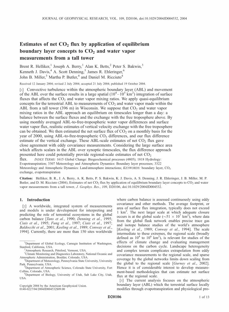
(and by inference, CO2) at the WLEF tower was on the orderof 106 km2, and other published estimates of surface areaaffecting scalar mixing ratios in the ABL range from 103 to105 km2 [Raupach et al., 1992; Styles et al., 2002]. Weassumed that EC estimates of Fq made from the tower werefairly representative of the region as a whole. However, itwould obviously be preferable to obtain estimates of Fq overa spatial scale that is representative of Cm and qm.[24] Figure 7 compares the EC local value of Fq with

monthly averages from the NCEP/NCAR reanalysis-2(surface footprint of about 3 � 104 km2). The two estimatesof Fq are closely matched for July through October. How-ever, for the rest of the year Fq from the reanalysis-2 dataappears to be unrealistically large. For example, in Marchand April when average temperatures are below freezing andthe deciduous trees have yet to flush leaves the Reanalysis Fqwas only about 25% less than August. Surface flux productsfrom different models and reanalyses show considerablevariability in the surface evaporation coming from differentland-surface models and analysis methods [Roads and Betts,2000; Roads et al., 2003; Berbery et al., 2003; Betts et al.,2003], so it is clear we do not yet have accurate regionalestimates of surface fluxes from models, although improve-ments are continually being made.[25] This success of the flux difference method suggests

that vertical exchange between the ABL and the freetroposphere dominates the continental ABL CO2 budgetover seasonal timescales. This vertical exchange explainsthe seasonal phase lag between ABL CO2 mixing ratios andNEE of CO2 noted in the WLEF data [Davis et al., 2003]and explored for multiple sites by Bakwin et al. [2004].Further, Bakwin et al. [2004] adopted a modification of ourmethod using only the reanalysis-2 data and extended itwith reasonable success to multiple sites, suggesting thatthese results are not unique to the northern Wisconsinregion.

3.5. Sensitivity Analysis

[26] The importance of each measured variable in calcu-lating FNEE using the flux difference method (rWFD) wasassessed individually by performing a sensitivity analysisover ‘‘all days’’ using the standard error of the mean for

Figure 6. Net ecosystem exchange for CO2 calculated using either the marine boundary layer (MBL) orNiwot Ridge (niwot) for free-tropospheric CO2. All calculations were made using the ppt < 1 filter. Seecolor version of this figure in the HTML.

D20106 HELLIKER ET AL.: BOUNDARY LAYER ESTIMATES OF CO2 FLUX

10 of 13

D20106

each variable (listed in Table 2). The standard error for eachmonth was calculated assuming that each 24 hour periodwas one independent sample for the monthly mean. Theresults of the sensitivity analysis are presented in Table 3.FNEE was least sensitive to qt, which is not surprising asfree-tropospheric water vapor from 2500 to 3200 m wasrelativel y constant and near 1.3 g kg �1 on an annual basis.Therefore a precise measurement of qm is more importantthan qt in calculating the water vapor difference between theABL and the free troposphere. The most important variablein matching FNEE to eddy covariance measurements of NEEwas Cm, followed by Fq, Ct and qm. Hence accuratemeasurements of Fq, qm and (Cm � Ct) are crucial to fluxcalculation by the ABL-flux method. Note that the standarderror of the mean for Cm and Ct was on the order ofmeasurement precision (0.1 ppmv).[27] The propagated errors associated with FNEE (Table 2)

and the sensitivity analysis (Table 3) are obviously only apartial consideration of the error involved in calculatingthe net flux. Our assumptions that Fq measured by ECrepresents regional Fq, and that Ct can be appropriatelyrepresented by the use of proxies rather than direct mea-surements represent potentially large sources of error forestimates of FNEE by the flux difference approach; errorsources which are not currently quantifiable. We used thereanalysis-2 data in an attempt to assuage the concern aboutasynchrony in Fq estimates, unfortunately the surface fluxfrom the reanalysis-2 data appears to be unrealistically largefor a part of the year. However, there are more robust land-coverage-based methods for estimating the largely unidi-rectional flux of water vapor for future tests of the fluxdifference method [Anderson et al., 1997, 2000; Mackay etal., 2002]. During storms water vapor is not conserved;however, both the surface flux and the water vapor differ-ence between the ABL and free troposphere are smallduring these periods. Although water vapor is used hereas the reference gas to obtain CO2 transport, other gasessuch as radon, which is produced in the soil, might be

another option. The representativeness of MBL proxies forCt can be confirmed by regular aircraft soundings over thecontinent which will be an integral component of the NorthAmerican Carbon Plan [Wofsy and Harris, 2002]. Further-more, caution is needed when comparing these results topublished eddy covariance flux estimates [e.g., Davis et al.,2003] since our calculations have not taken into accountperiod of missing data (14%) or times with low turbulence.The addition of data from more terrestrial towers andregular airplane flights, in concert with atmospheric trans-port models of free-tropospheric CO2, would no doubt helpconstrain regional estimates of FNEE.

4. Conclusions

[28] By approaching average CO2 and water vapor mix-ing ratios in the ABL as a quasi-equilibrium problem, andmaking some simple assumptions about free-tropospheric

Table 3. Sensitivity Analysis for FNEE-FDa

Month

Percent Change From Estimated FNEE All Days

Fq + sem Ct + sem Cm + sem qt + sem qm + sem

Jan. 25 4 12 2 11Feb. 20 3 8 1 12Mar. 10 3 13 1 11Apr. 9 9 10 2 7May 8 14 56 1 6June 9 3 13 1 5July 8 4 8 1 4Aug. 8 4 16 0 0Sep. 9 13 29 1 6Oct. 11 2 15 1 8Nov. 19 3 7 2 7Dec. 15 6 13 2 7Mean (year) 13 6 17 1 7Mean (May–Sep.) 8 7 24 1 4

aOne standard error was added to each input individually while holdingthe other inputs constant to calculate the percent change in FNEE relative tothe FNEE-FD values presented in Figure 5.

Figure 7. Monthly averages of molar water vapor flux (Fq) measured by eddy covariance at 122 m(blue triangles) on the WLEF tower and from NCEP/NCAR reanalysis-2 data (red diamonds). See colorversion of this figure in the HTML.

D20106 HELLIKER ET AL.: BOUNDARY LAYER ESTIMATES OF CO2 FLUX

11 of 13

D20106

boundary conditions, we were able to estimate net CO2

surface exchange for an entire year from surface measure-ments of evaporation. These ABL-scale net CO2 estimateswere comparable to measurements made by eddy covari-ance techniques over this same time period. This lendsobservational support to the underlying hypothesis outlinedin the introduction: that on timescales longer than a day andin subsiding regimes the ABL structure of water vapor andCO2 represents a near-balance between the surface fluxesand the mixing-down of air from the free troposphere, andthe fluxes can be represented by a mass exchange with thefree troposphere and the difference of CO2 and water vaporbetween the ABL and the free troposphere. It is obvious,however, that the full potential of this method requires morecomplete and systematic data, especially for CO2 and watervapor in the free troposphere. New global and regionalreanalyzes may also provide better regional estimates ofsurface evaporation for comparison with eddy correlationdata. Recognizing the large surface area which affectsscalars in the ABL over synoptic timescales, the fluxdifference approach presented here could provide usefulregional- to continental-scale observational constraints onthe net surface CO2 flux for comparison with modelestimates.

Appendix A

[29] The 396 m measurement height of Cm is generallyabove the nocturnal inversion and is nearly always belowthe capping inversion separating the ABL from theoverlying free troposphere. Continuous measurementsfrom this height, therefore, reflect changes in the daytimeconvective boundary layer and the nighttime residuallayer through time @Cm

@t

� �[Yi et al., 2001]. Cotton et al.

[1995] showed that is a on a global average ABL air isreplaced by free-tropospheric air every four days, so onthese longer timescales, we assume that horizontal advec-tion becomes less important than vertical advection andmixing across the substantial jump in CO2 concentrationassociated with the capping inversion of the ABL. Wetherefore use a simplified budget equation for the ABLwith depth h and mean CO2 concentration Cm in whichwe neglect horizontal advection. As the ABL deepens ina subsiding mean flow W it entrains air from the freetroposphere above with properties Ct, and we can writethe budget equation for the ABL as [Betts, 1992]

@

@trhCmð Þ ¼ FNEE þ r

@h

@t

� �Ct � rW Ct � Cmð Þ; ðA1Þ

where FNEE is the net surface CO2 flux (Fphotosynthesis +Frespiration) in flux density units. Rearranging and ignoringthe time variation of r gives

rh@Cm

@t¼ FNEE � rW Ct � Cmð Þ; ðA2Þ

where W ¼ @h@t

� ��W is the entrainment rate of the ABL,

or the rate at which the ABL mixes in air from the freetroposphere (W is typically negative corresponding to

mean subsidence). In strict equilibrium, @Cm@t = @h

@t = 0 andwe get

FNEE ¼ rW Ct � Cmð Þ ¼ rW Ct � Cmð Þ: ðA3Þ

A similar equation to equation (A2) can be written forwater vapor

rh@qm@t

¼ Fq � rW qt � qmð Þ: ðA4Þ

Following Raupach et al. [1992], we can assume a similarABL entrainment rate for C and q. Dividing equation(A2) by equation (A4), and neglecting the time rate ofchange terms @Cm

@t ; @qm@t

� �which become small compared to

the flux terms over longer averaging periods (seeTable A1) gives

FNEE ¼Ct � Cm

� �qt � qmð Þ � Fq: ðA5Þ

[30] Acknowledgments. We are grateful to D. Fitzjarrald, R. Strand,P. Tans, R. Teclaw, S. Wofsy for theoretical and technical help with thisstudy and the State of Wisconsin Educational Communications Board foraccess to the WLEF tower. This work was supported by grants from theNational Oceanic and Atmospheric Administration (NAO6-GP-409), theNational Science Foundation (TECO; DEB-9814194) and the Departmentof Energy (NIGEC; DEFC03-90ER61010 and DOE/DE-FG02-97ER62457). AKB was supported by NSF (ATM-9988618) and NASA(NAG5-11578).

ReferencesAnderson, M. C., J. M. Norman, G. R. Diak, W. P. Kustas, and J. R.Mecikalski (1997), A two-source time-integrated model for estimatingsurface fluxes using thermal infrared remote sensing, Remote Sens.Environ., 60, 195–216.

Anderson, M. D., J. M. Norman, T. P. Meyers, and G. R. Diak (2000),An analytical model for estimating canopy transpiration and carbonassimilation fluxes based on canopy light-use efficiency, Agric. For.Meteorol., 101, 265–289.

Bakwin, P. S., P. P. Tans, D. F. Hurst, and C. Zhao (1998), Measurementsof carbon dioxide on very tall towers: Results of the NOAA/CMDLprogram, Tellus, Ser. B, 50, 401–415.

Bakwin, P. S., K. J. Davis, C. Yi, S. C. Wofsy, J. W. Munger, L. Haszpra,and Z. Barcza (2004), Regional carbon dioxide fluxes from mixing ratiodata, Tellus, Ser. B, 56, 301–311.

Baldocchi, D., et al. (2001), FLUXNET: A new tool to study the temporaland spatial variability of ecosystem-scale carbon dioxide, water vaporand energy flux densities, Bull. Am. Meteorol. Soc., 82, 2415–2434.

Berbery, E. H., Y. Luo, K. E. Mitchell, and A. K. Betts (2003), Etamodel estimated land surface processes and the hydrologic cycle of theMississippi basin, J. Geophys. Res., 108(D22), 8852, doi:10.1029/2002JD003192.

Betts, A. K. (1992), FIFE atmospheric boundary layer budget methods,J. Geophys. Res., 97, 18,523–18,532.

Betts, A. K. (2000), Idealized model for equilibrium boundary layer overland, J. Hydrometeorol., 1, 507–523.

Betts, A. K. (2004), Understanding hydrometeorology using global models:American Meteorological Society Robert Horton Lecture, E., January 14,2004, Seattle, Bull. Am. Meteorol. Soc., in press.

Table A1. Rate of Change and Flux Terms for CO2 and H2O as

the Averaging Period Increasesa

FNEE,mmol m�2 s�1

@Cm@t h,

mmol m�2 s�1Fq,

mmol m�2 s�1

@qm@t h,

mmol m�2 s�1

Sequence(2–7 Aug.)

�1.42 0.21 2.31 0.03

Aug. �1.79 0.02 2.03 0.01June–Aug. �1.80 �0.06 2.18 0.02

aAssuming mean h of 1500 m.

D20106 HELLIKER ET AL.: BOUNDARY LAYER ESTIMATES OF CO2 FLUX

12 of 13

D20106

Betts, A. K., and J. H. Ball (1998), FIFE surface climate and site-averagedataset 1987–89, J. Atmos. Sci., 55, 1091–1108.

Betts, A. K., and W. L. Ridgway (1989), Climatic equilibrium of the atmo-spheric convective boundary layer over a tropical ocean, J. Atmos. Sci.,46, 2621–2641.

Betts, A. K., J. H. Ball, M. Bosilovich, P. Viterbo, Y. Zhang, and W. B.Rossow (2003), Intercomparison of water and energy budgets for fiveMississippi subbasins between ECMWF reanalysis (ERA-40) and NASAData Assimilation Office fvGCM for 1990–1999, J. Geophys. Res.,108(D16), 8618, doi:10.1029/2002JD003127.

Betts, A. K., B. R. Helliker, and J. A. Berry (2004), Coupling betweenCO2, water vapor, temperature and radon and their fluxes in an idealizedequilibrium boundary layer over land, J. Geophys. Res., 109, D18103,doi:10.1029/2003JD004420.

Ciais, P., P. P. Tans, M. Trolier, J. W. C. White, and R. J. Francey (1995), Alarge Northern Hemisphere terrestrial CO2 sink indicated by the 13C/12Cratio of atmospheric CO2, Science, 269, 1098–1102.

Ciais, P., et al. (1997), A three-dimensional synthesis study of d18O inatmospheric CO2: 2. Simulations with the TM2 transport model, J. Geo-phys. Res., 102, 5873–5883.

Conway, T. J., P. P. Tans, L. S. Waterman, K. W. Thoning, D. R. Kitzis,K. A. Masarie, and N. Zhang (1994), Evidence for interannual variabilityof the carbon cycle from the National Oceanic and Atmospheric Admin-istration/Climate Monitoring and Diagnostics Laboratory Global AirSampling Network, J. Geophys. Res., 99(D11), 22,831–22,855.

Cotton, W. R., G. D. Alexander, R. Hertenstein, R. L. Walko, R. L.McAnelly, and M. Nicholls (1995), Cloud venting—A review and somenew global annual estimates, Earth Sci. Rev., 39, 169–206.

Davis, K. J., P. S. Bakwin, B. W. Berger, C. Yi, C. Zhao, R. M. Teclaw, andJ. G. Isebrands (2003), Long-term carbon dioxide fluxes from a very talltower in a northern forest: Annual cycle of CO2 exchange, GlobalChange Biol., 9, 1278–1293.

De Bruin, H. A. R. (1983), A model for the Priestley-Taylor parameter, a,J. Clim. Appl. Meteorol., 22, 572–578.

Denmead, O. T., M. R. Raupach, F. X. Dunin, H. A. Cleugh, and R. Leuning(1996), Boundary layer budgets for regional estimates of scalar fluxes,Global Change Biol., 2, 255–264.

Denning, A. S., I. Y. Fung, and D. Randall (1995), Latitudinal gradient ofatmospheric CO2 due to seasonal exchange with land biota, Nature, 376,240–243.

Fan, S., M. Gloor, J. Mahlman, S. Pacala, J. Sarmiento, T. Takahashi, andP. Tans (1998), A large terrestrial carbon sink in North America impliedby atmospheric and oceanic carbon dioxide data and models, Science,282, 442–446.

Fitzjarrald, D. R. (2002), Boundary layer budgeting, in Vegetation, Water,Humans and the Climate: A New Perspective on an Interactive System,edited by P. Kabat et al., pp. 239–254, Springer-Verlag, New York.

Fung, I., et al. (1997), Carbon 13 exchanges between the atmosphere andbiosphere, Global Biogeochem. Cycles, 11, 507–533.

Gerbig, C., J. C. Lin, S. C. Wofsy, B. C. Daube, A. E. Andrews, B. B.Stephens, P. S. Bakwin, and A. Grainger (2003), Toward constrainingregional-scale fluxes of CO2 with atmospheric observations over acontinent: 1. Observed spatial variability from airborne platforms,J. Geophys. Res., 108(D24), 4756, doi:10.1029/2002JD003018.

Gloor, M., P. Bakwin, D. Hurst, L. Lock, R. Draxler, and P. Tans (2001),What is the concentration footprint of a tall tower?, J. Geophys. Res.,106(D16), 17,831–17,840.

Gurney, K. J., et al. (2002), Towards robust regional estimates of CO2sources and sinks using atmospheric transport models, Nature, 415,626–630.

Helliker, B. R., J. Berry, P. Bakwin, K. Davis, A. S. Denning, J. Ehleringer,J. Miller, M. Butler, and D. Ricciuto (2002), Measurements of regional-scale isotopic discrimination and CO2 flux for the north-central U.S., EosTrans. AGU, 83, Fall Meet. Suppl., Abstract B71C-10.

Hurwitz, M. D., D. M. Ricciuto, K. J. Davis, W. Wang, C. Yi, M. P. Butler,and P. S. Bakwin (2004), Advection of carbon dioxide in the presence ofstorm systems over a northern Wisconsin forest, J. Atmos. Sci., 61, 607–618.

Keeling, C. D., et al. (1989), A three-dimensional model of atmosphericCO2 transport based on observed winds: 1. Analysis of observationaldata, in Aspects of Climate Variability in the Pacific and the WesternAmericas, Geophys. Monogr. Ser., vol. 55, edited by D. H. Peterson,pp. 277–303, AGU, Washington, D. C.

King, D. B., and R. C. Schnell (Eds.) (2002), Climate monitoring anddiagnostics laboratory summary, Rep. 26, 2000–2001, NOAA/CMDL,Boulder, Colo.

Kuck, L. R., et al. (2000), Measurements of landscape-scale fluxes ofcarbon dioxide in the Peruvian Amazon by vertical profiling throughthe atmospheric boundary layer, J. Geophys. Res., 105(D17), 2137–2146.

Levy, P. E., A. Grelle, A. Lindroth, M. Molder, P. G. Jarvis, B. Kruijt, andJ. B. Moncrieff (1999), Regional-scale CO2 fluxes over central Swedenby a boundary layer budget method, Agric. For. Meteorol., 99, 169–180.

Lloyd, J., et al. (2001), Vertical profiles, boundary layer budgets, andregional flux estimates for CO2 and its 13C/12C ratio and for water vaporabove a forest/bog mosaic in central Siberia, Global Biogeochem. Cycles,15(2), 267–284.

Mackay, D. S., D. E. Ahl, B. E. Ewers, S. T. Gower, S. N. Burrows,S. Samanta, and K. J. Davis (2002), Effects of aggregated classificationsof forest composition on estimates of evapotranspiration in a northernWisconsin forest, Global Change Biol., 8(12), 1253–1265.

McNaughton, K. G., and T. W. Spriggs (1986), A mixed-layer model forregional evaporation, Boundary Layer Meteorol., 34, 243–262.

Pattey, E., I. B. Strachan, R. L. Desjardins, and J. Massheder (2002),Measuring nighttime CO2 flux over terrestrial ecosystems using eddycovariance and nocturnal boundary layer methods, Agric. For. Meteorol.,113, 145–158.

Peixoto, J. P., and A. H. Oort (1992), Physics of Climate, Springer-Verlag,New York.

Raupach, M. R. (1995), Vegetation-atmosphere interaction and surface con-ductance at leaf, canopy and regional scales, Agric. Forest Meteorol., 73,151–170.

Raupach, M. R. (2000), Equilibrium evaporation and the convective bound-ary layer, Boundary Layer Meteorol., 96, 107–141.

Raupach, M. R. (2001), Combination theory and equilibrium evaporation,Q. J. R. Meteorol. Soc., 127, 1149–1181.

Raupach, M. R., O. T. Denmead, and F. X. Dunin (1992), Challenges inlinking atmospheric CO2 concentrations to fluxes at local and regionalscales, Aust. J. Botany, 40, 697–716.

Roads, J., and A. K. Betts (2000), NCEP/NCAR and ECMWF reanalysissurface water and energy budgets for the GCIP region, J. Hydrometeorol.,1, 88–94.

Roads, J., et al. (2003), GCIP Water and Energy Budget Synthesis (WEBS),J. Geophys. Res., 108(D16), 8609, doi:10.1029/2002JD002583.

Stull, R. B. (1988), An Introduction to Boundary Layer Meteorology,666 pp., Kluwer Acad., Norwell, Mass.

Styles, J. M., J. Lloyd, D. Zolotoukhine, K. A. Lawton, N. Tchebakova,R. J. Francey, A. Arneth, D. Salamakho, O. Kolle, and E.-D. Schulze(2002), Estimates of regional surface carbon dioxide exchange andcarbon and oxygen isotope discrimination during photosynthesis fromconcentration profiles in the atmospheric boundary layer, Tellus, Ser. B,54, 768–783.

Tans, P. P., I. Y. Fung, and T. Takahashi (1990), Observational constraintson the global atmospheric CO2 budget, Science, 247, 1431–1438.

Wofsy, S. C., and R. C. Harris (2002), The North American CarbonProgram (NACP): Report of the NACP Committee of the U.S. Inter-agency Carbon Cycle Science Program, U.S. Global Change Res.Program, Washington, D. C.

Yi, C., K. J. Davis, and B. W. Berger (2001), Long-term observations of thedynamics of the continental planetary boundary layer, J. Atmos. Sci., 58,1288–1299.

Yi, C., K. J. Davis, P. S. Bakwin, A. S. Denning, N. Zhang, A. Desai, J. C.Lin, and C. Gerbig (2004), Observed covariance between ecosystemcarbon exchange and atmospheric boundary layer dynamics at a site innorthern Wisconsin, J. Geophys. Res., 109, D08302, doi:10.1029/2003JD004164.

�����������������������P. S. Bakwin and J. B. Miller, Climate Monitoring and Diagnostics

Laboratory, National Oceanic and Atmospheric Administration, 325Broadway R/CMDL1, Boulder, CO 80305, USA.J. A. Berry and B. R. Helliker, Department of Global Ecology, Carnegie

Institution of Washington, 260 Panama St., Stanford, CA 94305, USA.(helliker@catalase.stanford.edu)A. K. Betts, Atmospheric Research, Pittsford, VT 05763, USA.M. P. Butler, K. J. Davis, and D. M. Ricciuto, Department of

Meteorology, Pennsylvania State University, 512 Walker Building,University Park, PA 16802, USA.A. S. Denning, Department of Atmospheric Science, Colorado State

University, Fort Collins, CO 80523, USA.J. R. Ehleringer, Department of Biology, University of Utah, 257S.

1400E., Salt Lake City, UT 84112, USA.

D20106 HELLIKER ET AL.: BOUNDARY LAYER ESTIMATES OF CO2 FLUX

13 of 13

D20106